Predicting Attention Sparsity in Transformers

Abstract

Transformers’ quadratic complexity with respect to the input sequence length has motivated a body of work on efficient sparse approximations to softmax. An alternative path, used by entmax transformers, consists of having built-in exact sparse attention; however this approach still requires quadratic computation. In this paper, we propose Sparsefinder, a simple model trained to identify the sparsity pattern of entmax attention before computing it. We experiment with three variants of our method, based on distances, quantization, and clustering, on two tasks: machine translation (attention in the decoder) and masked language modeling (encoder-only). Our work provides a new angle to study model efficiency by doing extensive analysis of the tradeoff between the sparsity and recall of the predicted attention graph. This allows for detailed comparison between different models along their Pareto curves, important to guide future benchmarks for sparse attention models.

1 Introduction

Transformer-based architectures have achieved remarkable results in many NLP tasks (Vaswani et al., 2017; Devlin et al., 2019; Brown et al., 2020). However, they also bring important computational and environmental concerns, caused by their quadratic time and memory computation requirements with respect to the sequence length. This comes in addition to the difficulty of interpreting their inner workings, caused by their overparametrization and large number of attention heads.

There is a large body of work developing ways to “sparsify” the computation in transformers, either by imposing local or fixed attention patterns (Child et al., 2019; Tay et al., 2020; Zaheer et al., 2020), by applying low-rank kernel approximations to softmax (Wang et al., 2020; Choromanski et al., 2021), or by learning which queries and keys should be grouped together Kitaev et al. (2019); Daras et al. (2020); Roy et al. (2021); Wang et al. (2021). Most of the existing work seeks to approximate softmax-based attention by ignoring the (predicted) tails of the distribution, which can lead to performance degradation. An exception is transformers with entmax-based sparse attention (Correia et al., 2019), a content-based approach which is natively sparse – this approach has the ability to let each attention head learn from data how sparse it should be, eliminating the need for heuristics or approximations. The disadvantage of this approach is that it still requires a quadratic computation to determine the sparsity pattern, failing to take computational advantage of attention sparsity.

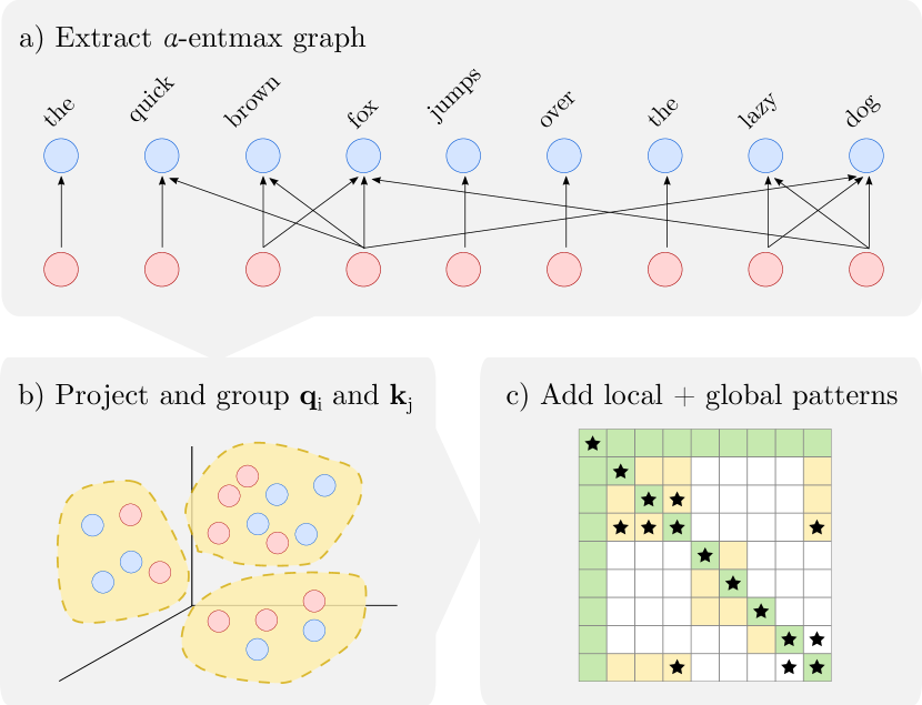
Figure 1: (a) Extract sparse attention graphs from a pretrained $\alpha$-entmax transformer; (b) Project query and key vectors to a smaller and appropriated space such that similar points are likely to fall in the same vicinity; (c) Additionally, we can combine window and global patterns (green blocks) with the learned pattern (yellow blocks) to increase the recall in recovering ground-truth edges from the sparse graph at the top (starred blocks).

In this paper, we propose Sparsefinder, which fills the gap above by making entmax attention more efficient (§4). Namely, we investigate three methods to predict the sparsity pattern of entmax without having to compute it: one based on metric learning, which is still quadratic but with a better constant (§4.3), one based on quantization (§4.4), and another based on clustering (§4.5). In all cases, the predictors are trained offline on ground-truth sparse attention graphs from an entmax transformer, seeking high recall in their predicted edges without compromising the total amount of sparsity. Figure 1 illustrates our method.

More precisely, to evaluate the effectiveness of our method across different scenarios, we perform experiments on two NLP tasks, encompassing encoder-only and decoder-only configurations: machine translation (MT, §5) and masked language modeling (MLM, §6), doing an extensive analysis of the tradeoff between sparsity and recall (i.e., performance on the attention graph approximation), and sparsity and accuracy (performance on downstream tasks). We compare our method with four alternative solutions based on efficient transformers: Longformer (Beltagy et al., 2020), Bigbird (Zaheer et al., 2020), Reformer (Kitaev et al., 2020), and Routing Transformer (Roy et al., 2021), along their entire Pareto curves. We complement these experiments by analyzing qualitatively what is selected by the different attention heads at the several layers and represented in different clusters/buckets. Overall, our contributions are:

• We propose a simple method that exploits learnable sparsity patterns to efficiently compute multi-head attention (§4).

• We do an extensive analysis of the tradeoff between sparsity and recall, and sparsity and accuracy in MT (§5) and MLM (§6), showing that there is clear room for improvement in the design of efficient transformers.

• We qualitatively analyze what is selected by the different attention heads at various layers and represented in different clusters/buckets.

2 Related Work

Interpreting multi-head attention.

Several works analyze the functionalities learned by different attention heads, such as positional and local context patterns (Raganato and Tiedemann, 2018; Voita et al., 2019). Building upon prior work on sparse attention mechanisms (Peters et al., 2019), Correia et al. (2019) constrain the attention heads to induce sparse selections individually for each head, bringing interpretability without post-hoc manipulation. Related approaches include the explicit sparse transformer (Zhao et al., 2019) and rectified linear attention (Zhang et al., 2021), which drops the normalization constraint. Raganato et al. (2020) show that it is possible to fix attention patterns based on previously known behavior (e.g. focusing on previous token) while improving translation quality. However, a procedure that exploits learnable sparsity patterns to accelerate multi-head attention is still missing.

Low-rank softmax approximations.

Methods based on low-rank approximation to the softmax such as Linearized Attention (Katharopoulos et al., 2020), Linformer (Wang et al., 2020), and Performer (Choromanski et al., 2021) reduce both speed and memory complexity of the attention mechanism from quadratic to linear, but make interpretability more challenging because the scores are not computed explicitly. On the other hand, methods that focus on inducing sparse patterns provide interpretable alignments and also have performance gains in terms of speed and memory.

Fixed attention patterns.

Among fixed pattern methods, Sparse Transformer (Child et al., 2019) and LongFormer (Beltagy et al., 2020) attend to fixed positions by using strided/dilated sliding windows. BigBird uses random and two fixed patterns (global and window) to build a block sparse matrix representation (Zaheer et al., 2020), taking advantage of block matrix operations to accelerate GPU computations. In contrast, we replace the random pattern with a learned pattern that mimics pretrained $\alpha$-entmax sparse attention graphs.

Learnable attention patterns.

Learnable pattern methods usually have to deal with assignment decisions within the multi-head attention mechanism. Clustered Attention (Vyas et al., 2020) groups query tokens into clusters and computes dot-products only with centroids. Reformer (Kitaev et al., 2020) and SMYRF (Daras et al., 2020) use locality-sensitive hashing to efficiently group tokens in buckets. More similar to our work, Routing Transformer (Roy et al., 2021) and Cluster-Former (Wang et al., 2021) cluster queries and keys with online k-means and compute dot-products over the top-k cluster points. Some queries and keys are discarded due to this filtering, which affects the overall recall of the method (as we show in §5 and §6). The ability of Routing Transformer to benefit from contextual information has been analyzed by Sun et al. (2021). In contrast, Sparsefinder learns to cluster based on sparsity patterns from attention graphs generated by $\alpha$-entmax.

3 Background

3.1 Transformers

The main component of transformers is the multi-head attention mechanism (Vaswani et al., 2017). Given as input a matrix $\mathbf{Q}\in\mathbb{R}^{n\times d}$ containing $d$-dimensional representations for $n$ queries, and matrices $\mathbf{K},\mathbf{V}\in\mathbb{R}^{m\times d}$ for $m$ keys and values, the scaled dot-product attention at a single head is computed in the following way:

$$\text{att}(\mathbf{Q},\mathbf{K},\mathbf{V})=\pi\underbrace{\Bigg{(}\frac{\mathbf{Q}\mathbf{K}^{\top}}{\sqrt{d}}\Bigg{)}}_{\mathbf{Z}\in\mathbb{R}^{n\times m}}\mathbf{V}\in\mathbb{R}^{n\times d}.$$ (1)

The $\pi$ transformation maps rows to distributions, with softmax being the most common choice, $\pi(\mathbf{Z})_{ij}=\mathrm{softmax}(\mathbf{z}_{i})_{j}$. Multi-head attention is computed by evoking Eq. 1 in parallel for each head $h$:

$$\text{head}_{h}(\mathbf{Q},\mathbf{K},\mathbf{V})=\text{att}(\mathbf{Q}\mathbf{W}^{Q}_{h},\mathbf{K}\mathbf{W}^{K}_{h},\mathbf{V}\mathbf{W}^{V}_{h}),$$

where $\mathbf{W}^{Q}_{h}$, $\mathbf{W}^{K}_{h}$, $\mathbf{W}^{V}_{h}$ are learned linear transformations. This way, heads are able to learn specialized phenomena. According to the nature of the input, transformers have three types of multi-head attention mechanism: encoder self-attention (source-to-source), decoder self-attention (target-to-target), and decoder cross-attention (target-to-source). While there are no restrictions to which elements can be attended to in the encoder, elements in position $j>i$ in the decoder self-attention are masked at timestep $i$ (“causal mask”).

3.2 Extmax Transformers and Learned Sparsity

The main computational bottleneck in transformers is the matrix multiplication $\mathbf{Q}\mathbf{K}^{\top}$ in Eq. 1, which costs $\mathcal{O}(nmd)$ time and can be impractical when $n$ and $m$ are large. Many approaches, discussed in §2, approximate Eq. 1 by ignoring entries far from the main diagonal or computing only some blocks of this matrix, with various heuristics. By doing so, the result will be an approximation of the softmax attention in Eq. 1. This is because the original softmax-based attention is dense, i.e., it puts some probability mass on all tokens – not only a computational disadvantage, but also making interpretation harder, as it has been observed that only a small fraction of attention heads capture relevant information (Voita et al., 2019).

An alternative to softmax is the $\alpha$-entmax transformation (Peters et al., 2019; Correia et al., 2019), which leads to sparse patterns directly, without any approximation:

$$\alpha\text{-entmax}(\mathbf{z})=[(\alpha-1)\mathbf{z}-\tau(\mathbf{z})\mathbf{1}]_{+}^{\nicefrac{{1}}{{\alpha-1}}},$$ (2)

where $[\cdot]_{+}$ is the positive part (ReLU) function, and $\tau:\mathbb{R}^{n}\rightarrow\mathbb{R}$ is a normalizing function satisfying $\sum_{j}[(\alpha-1)z_{j}-\tau(\mathbf{z})]_{+}^{\nicefrac{{1}}{{\alpha-1}}}=1$ for any $\mathbf{z}$. That is, entries with score $z_{j}\leq\nicefrac{{\tau(\mathbf{z})}}{{\alpha-1}}$ get exactly zero probability. In the limit $\alpha\rightarrow 1$, $\alpha$-entmax recovers the softmax function, while for any value of $\alpha>1$ this transformation can return sparse probability vectors (as the value of $\alpha$ increases, the induced probability distribution becomes more sparse). When $\alpha=2$, we recover sparsemax (Martins and Astudillo, 2016). In this paper, we use $\alpha=1.5$, which works well in practice and has a specialized fast algorithm (Peters et al., 2019).

Although sparse attention improves interpretability and head diversity when compared to dense alternatives (Correia et al., 2019), the learned sparsity patterns cannot be trivially exploited to reduce the quadratic burden of self-attention, since we still need to compute dot-products between all queries and keys ($\mathbf{Q}\mathbf{K}^{\top}$) before applying the $\alpha\text{-entmax}$ transformation. In the next section (§4), we propose a simple method that learns to identify these sparsity patterns beforehand, avoiding the full matrix multiplication.

4 Sparsefinder

We now propose our method to extract sparse attention graphs and learn where to attend by exploiting a special property of $\alpha$-entmax: sparse-consistency (§4.1). We design three variants of Sparsefinder to that end, based on metric learning (§4.3), quantization (§4.4), and clustering (§4.5).

4.1 Attention graph and sparse-consistency

For each attention head $h$, we define its attention graph as $\mathcal{G}_{h}=\{(\mathbf{q}_{i},\mathbf{k}_{j})\mid p_{i,j}>0\}$, a bipartite graph connecting query and key pairs $\mathbf{q}_{i},\mathbf{k}_{j}\in\mathbb{R}^{d}$ for which the $\alpha\text{-entmax}$ probability $p_{i,j}$ is nonzero. An example of attention graph is shown in Figure 1. We denote by $|\mathcal{G}_{h}|$ the total size of an attention graph, i.e., its number of edges. With $\alpha\text{-entmax}$ with $\alpha=1.5$ we typically have $|\mathcal{G}_{h}|\ll nm$. In contrast, softmax attention always leads to a complete graph, $|\mathcal{G}_{h}|=nm$.

Problem statement.

Our goal is to build a model – which we call Sparsefinder – that predicts $\hat{\mathcal{G}}_{h}\approx\mathcal{G}_{h}$ without having to perform all pairwise comparisons between queries and keys. This enables the complexity of evaluating Eq. 1 to be reduced from $\mathcal{O}(nmd)$ to $\mathcal{O}(|\hat{\mathcal{G}}_{h}|d)$, effectively taking advantage of the sparsity of $\alpha$-entmax. In order to learn such a model, we first extract a dataset of sparse attention graphs $\{\mathcal{G}_{h}\}$ from a pretrained entmax-based transformer, which acts as a teacher. Then, the student learns where to pay attention based on this information. This procedure is motivated by the following sparse-consistency property of $\alpha$-entmax:

Proposition 1 (Sparse-consistency property).

Let $\mathbf{b}$ be a binary vector such that $b_{j}=1$ if $p_{j}^{\star}>0$, and $b_{j}=0$ otherwise. For any binary mask vector $\mathbf{m}$ “dominated” by $\mathbf{b}$ (i.e. $\mathbf{m}\odot\mathbf{b}=\mathbf{b}$), we have

$$\alpha\text{-entmax}(\mathbf{z})=\alpha\text{-entmax}(\mathbf{z}|_{\mathbf{m}}),$$ (3)

where $z_{j}|_{\mathbf{m}}=z_{j}$ if $m_{j}=1$ and $-\infty$ if $m_{j}=0$.

Proof.

See §A in the supplemental material. ∎

This property ensures that, if $\hat{\mathcal{G}}_{h}$ is such that $\mathcal{G}_{h}\subseteq\hat{\mathcal{G}}_{h}$, then we obtain exactly the same result as with the original entmax attention. Therefore, we are interested in having high recall,

$$\mathrm{recall}(\hat{\mathcal{G}}_{h};\mathcal{G}_{h})=\frac{|\hat{\mathcal{G}}_{h}\cap\mathcal{G}_{h}|}{|\mathcal{G}_{h}|},$$ (4)

meaning that our method is nearly exact, and high sparsity,

$$\mathrm{sparsity}(\hat{\mathcal{G}}_{h})=1-\frac{|\hat{\mathcal{G}}_{h}|}{nm},$$ (5)

which indicates that computation can be made efficient. Although a high sparsity may indicate that many computations can be ignored, converting this theoretical result into efficient computation is not trivial and potentially hardware-dependent. In this paper, rather than proposing a practical computational efficient method, we focus on showing that such methods do exist and that they can be designed to outperform fixed and learned pattern methods while retaining a high amount of sparsity when compared to the ground-truth graph.

Our strategies.

We teach the student model to predict $\hat{\mathcal{G}}_{h}\approx\mathcal{G}_{h}$ by taking inspiration from the Reformer model (Kitaev et al., 2020) and the Routing Transformer (Roy et al., 2021). Formally, we define a set of $B$ buckets, $\mathcal{B}=\{1,\ldots,B\}$, and learn functions $f_{q},f_{k}:\mathbb{R}^{d}\rightarrow 2^{\mathcal{B}}\setminus\{\varnothing\}$, which assign a query or a key to one or more buckets. We will discuss in the sequel different design strategies for the functions $f_{q},f_{k}$. Given these functions, the predicted graph is:

$$\hat{\mathcal{G}}_{h}=\{(\mathbf{q}_{i},\mathbf{k}_{j})\mid f_{q}(\mathbf{q}_{i})\cap f_{k}(\mathbf{k}_{j})\neq\varnothing\},$$ (6)

that is, an edge is predicted between $\mathbf{q}_{i}$ and $\mathbf{k}_{j}$ iff they are together in some bucket.

We present three strategies, based on distance-based pairing (§4.3), quantization (§4.4) and clustering (§4.5). As a first step, all strategies require learning a metric that embeds the graph (projecting queries and keys) into a lower-dimensional space $\mathbb{R}^{r}$ with $r\ll d$, such that positive query-key pairs are close to each other, and negative pairs are far apart.

4.2 Learning projections

According to the $\alpha$-entmax sparse-consistency property, in order to get a good approximation of $\mathcal{G}_{h}$, we would like that $f_{q}$ and $f_{k}$ produce a graph $\hat{\mathcal{G}}_{h}$ that maximizes recall, defined in Eq. 4. However, maximizing recall in this setting is difficult since we do not have ground-truth bucket assignments. Instead, we recur to a contrastive learning approach by learning projections via negative sampling, which is simpler and more scalable than constrained clustering approaches (Wagstaff et al., 2001; de Amorim, 2012).

For each head, we start by projecting the original query and key $\mathbf{q},\mathbf{k}\in\mathbb{R}^{d}$ vectors into lower dimensional vectors $\mathbf{q}^{\prime},\mathbf{k}^{\prime}\in\mathbb{R}^{r}$ such that $r\ll d$. In practice, we use a simple head-wise linear projection for all queries and keys $g_{\theta}:\mathbb{R}^{d}\rightarrow\mathbb{R}^{r}$. To learn the parameters of the projection layer we minimize a hinge loss with margin $\omega$ for each head $h$:

$$\mathcal{L}_{\theta}(\mathcal{G}_{h})=\Big{[}\omega+\|\mathbf{q}^{\prime}-\mathbf{k}^{\prime}_{\text{P}}\|^{2}_{2}-\|\mathbf{q}^{\prime}-\mathbf{k}^{\prime}_{\text{N}}\|^{2}_{2}\Big{]}_{+},$$ (7)

where $(\mathbf{q}^{\prime},\mathbf{k}_{\text{P}}^{\prime})\in\mathcal{G}_{h}$ is a positive pair and $(\mathbf{q}^{\prime},\mathbf{k}_{\text{N}}^{\prime})\notin\mathcal{G}_{h}$ is a negative pair sampled uniformly at random. In words, we want the distance between a query vector to negative pairs to be larger than the distance to positive pairs by a margin $\omega$. This approach can also be seen as a weakly-supervised learning problem, where the goal is to push dissimilar points away while keeping similar points close to each other (Xing et al., 2002; Weinberger and Saul, 2009; Bellet et al., 2015).

4.3 Distance-based pairing

To take advantage of the proximity of data points on the embedded space, we first propose a simple method to connect query and key pairs whose Euclidean distance is less than a threshold $t$, i.e. $\hat{\mathcal{G}}_{h}=\{(\mathbf{q}_{i},\mathbf{k}_{j})\mid\|\mathbf{q}^{\prime}_{i}-\mathbf{k}^{\prime}_{j}\|_{2}\leq t\}$. Although this method also requires $O(n^{2})$ computations, it is more efficient than a vanilla transformer since it reduces computations by a factor of $d/r$ by using the learned projections. This method is also useful to probe the quality of the embedded space learned by the projections, since the recall of our other methods will be contingent on it.

4.4 Buckets through quantization

Our second strategy quantizes each dimension $1,\dots,r$ of the lower-dimensional space into $\beta$ bins, placing the queries and keys into the corresponding buckets ($B=r\beta$ buckets in total). This way, each $\mathbf{q}_{i}$ and $\mathbf{k}_{j}$ will be placed in exactly $r$ buckets (one per dimension). If $\mathbf{q}_{i}$ and $\mathbf{k}_{j}$ are together in some bucket, Sparsefinder predicts that $(\mathbf{q}_{i},\mathbf{k}_{j})\in\hat{\mathcal{G}}_{h}$. Note that for this quantization strategy no learning is needed, only the hyperparameter $\beta$ and the binning strategy need to be chosen. We propose a fixed-size binning strategy: divide each dimension into $\beta$ bins such that all bins have exactly $\lceil n/\beta\rceil$ elements. In practice, we append padding symbols to the input to ensure that bins are balanced.

4.5 Buckets through clustering

The clustering strategy uses the low-dimensional projections and runs a clustering algorithm to assign $\mathbf{q}_{i}$ and $\mathbf{k}_{j}$ to one or more clusters. In this case, each cluster corresponds to a bucket. In our paper, we employed $k$-means to learn $B$ centroids $\{\mathbf{c}_{1},\ldots,\mathbf{c}_{B}\}$, where each $c_{b}\in\mathbb{R}^{r}$, over a small portion of the training set. This strategy is similar to the Routing Transformer’s online $k$-means (Roy et al., 2021), but with two key differences: (a) our clustering step is applied offline; (b) we assign points to the top-$k$ closest centroids rather than assigning the closest top-$k$ closest points to each centroid, ensuring that all queries are assigned to a cluster. At test time, we use the learned centroids to group queries and keys into $k$ clusters each:

$$f_{q}(\mathbf{q}_{i}) =\operatorname*{\text{arg\,top-$k$}}_{1\leq b\leq B}-\|\mathbf{q}_{i}-\mathbf{c}_{b}\|^{2}_{2},$$ (8)

$$f_{k}(\mathbf{k}_{j}) =\operatorname*{\text{arg\,top-$k$}}_{1\leq b\leq B}-\|\mathbf{k}_{j}-\mathbf{c}_{b}\|^{2}_{2},$$ (9)

where the $\operatorname*{\text{arg\,top-$k$}}$ operator returns the indices of the $k\textsuperscript{th}$ largest elements. As in the quantization-based approach, queries and keys will attend to each other, i.e., Sparsefinder predicts $(\mathbf{q}_{i},\mathbf{k}_{j})\in\hat{\mathcal{G}}_{h}$ if they share at least one cluster among the $k$ closest ones. Smaller values of $k$ will induce high sparsity graphs, whereas a larger $k$ is likely to produce a denser graph but with a higher recall.

4.6 Computational cost

Let $L$ be the maximum number of elements in a bucket. The time and memory cost of bucketed attention computed through quantization or clustering is $\mathcal{O}(BL^{2})$. With balanced buckets, we get a complexity of $\mathcal{O}(n^{1.5})$ by setting $B=\sqrt{n}$. Although this cost is sub-quadratic, leveraging the sparse structure of $\hat{\mathcal{G}}_{h}$ in practice is challenging, since it might require specialized hardware or kernels. In general, we have $|\hat{\mathcal{G}}_{h}|=\sum_{b=1}^{B}n_{b}m_{b}\ll nm$, where $n_{b}$ and $m_{b}$ are the number of queries and keys in each bucket, since we have small complete bipartite graphs on each bucket. Instead of viewing quadratic methods only in light of their performance, we adopt an alternative view of assessing the tradeoff of these methods in terms of sparsity and recall of their approximation $\hat{\mathcal{G}}_{h}$. This offers a theoretical perspective to the potential performance of each approximation on downstream tasks, helping to find the best approximations for a desired level of sparsity.

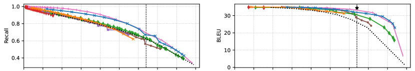
Figure 2: Sparsity-recall (left) and sparsity-BLEU (right) tradeoff averaged across all layers and heads on IWSLT en$\to$de (top) and en$\to$fr (bottom). The vertical dashed line represents the gold sparsity obtained by the original $\alpha$-entmax transformer (which requires quadratic computation), and the starred marks depict its BLEU score: $34.47$ on en$\to$de and $42.65$ on en$\to$fr.

4.7 Combining learned and fixed patterns

As pointed out in prior work (Voita et al., 2019), several attention heads rely strongly in local patterns or prefer to attend to a particular position, more promimently in initial layers. Therefore, we take inspiration from the Longformer Beltagy et al. (2020) and BigBird Zaheer et al. (2020) and combine learned sparse patterns with window and global patterns by adding connections in the predicted graph $\hat{\mathcal{G}}_{h}$ to improve the recall of all methods. Figure 1 illustrates how these patterns are combined in the last step.

5 Experiments: Machine Translation

Setup.

We pretrain a transformer-large model (6 layers, 16 heads) on the Paracrawl dataset (Esplà et al., 2019). Next, we finetune it with $\alpha$-entmax, fixing $\alpha=1.5$ for all heads, on en$\to$de and en$\to$fr language pairs from IWSLT17 (Cettolo et al., 2017). We use the 2011-2014 sets as validation data and the 2015 set as test data. We encode each word using byte pair encoding (BPE, Sennrich et al. 2016) with a joint segmentation of 32k merges. As Vaswani et al. (2017), we finetune our models using the Adam optimizer with an inverse square root learning rate scheduler, with an initial value of $5\times 10^{-4}$ and a linear warm-up in the first $4000$ steps. We evaluate translation quality with sacreBLEU (Post, 2018). Training details, hyperparameters, and data statistics are described in §C.

Learning projections.

To learn projections for queries and keys (§4.2), we randomly selected 10K long instances ($n>20$ tokens) from the training set and extracted the $\alpha\text{-entmax}$ attention graphs $\mathcal{G}_{h}$ from the decoder self-attention for each head. This led to an average of 8M and 9M positive pairs ($\mathbf{q}_{i},\mathbf{k}_{j}$) per layer for en$\to$de and en$\to$fr, respectively. In practice, due to the small number of parameters for each head (only 4,160), a single epoch with Adam was sufficient to optimize the loss in Eq. 7. The hyperparameters and the training details for learning projections can be found in §C.

Pareto-curves.

Using the learned projections, we investigate the recall and the accuracy of all Sparsefinder variants by comparing them with Longformer, BigBird, Reformer, and Routing Transformer. To get a fair comparison, we analyze each method for different levels of sparsity by varying the following hyperparameters:

• Distance-based methods: the threshold $t$ within $\{0.5,1.0,1.5,2.0,2.5,3.0,3.5,4.0,4.5,5.0\}$.

• Bucketing-based methods: the number of buckets $B$ within $\{2,4,6,8,10,12,16,20\}$.

• Fixed-pattern methods: the number of random blocks of size 1 within $\{2,4,6,8,10,12,16,20\}$ for BigBird; and the number of random global tokens within $\{2,4,6,8,10,12,16,20\}$ for Longformer.

We also add global and local patterns to all methods, varying the window size within $\{0,1,3,5,7,9,11,15,19,23,27\}$ to get different levels of locality. We further compare all methods with a simple window baseline that only induces the window and global patterns. Since all methods exhibit a tradeoff between sparsity and recall/accuracy, we plot the scores obtained by varying the hyperparameters and draw their respective Pareto frontier to see the optimal Pareto-curve. Methods whose points lie below this frontier are said to be Pareto-dominated, meaning that their recall/accuracy cannot be increased without sacrificing sparsity, or vice-versa. Concretely, each point on the curve is measured as a function of the approximation to the ground-truth $\alpha$-entmax attention graph $\mathcal{G}_{h}$ by replacing it by $\hat{\mathcal{G}}_{h}$ at test time.

Sparsity-recall tradeoff.

Pareto-curves for the sparsity-recall tradeoff are shown on the left of Figure 2 for both language pairs. Overall, both language pairs have similar trends for all methods. Sparsefinder’s distance-based and clustering approaches Pareto-dominates the other methods, followed by Routing Transformer. Interestingly, Longformer, BigBird, Routing Transformer, and Sparsefinder’s bucketing approach perform on par with the baseline, indicating that a simple local window is a hard baseline to beat. Since the LSH attention in Reformer shares queries and keys before hashing, the resultant buckets are also shared for queries and keys, explaining the high recall and the low sparsity of Reformer.

Sparsity-accuracy tradeoff.

We show the tradeoff between sparsity and BLEU on the right of Figure 2. For lower levels of sparsity, all methods perform well, close to the full entmax transformer. But as sparsity increases, indicating that only a few computations are necessary, we see that the distance-based and $k$-means variants of Sparsefinder Pareto-dominate other methods, keeping a very high BLEU without abdicating sparsity. In particular, Sparsefinder’s distance and clustering approaches perform on par with the full entmax transformer when the amount of sparsity is close to the original entmax transformer (around the vertical dashed line). Overall, these plots show that methods with a high recall for higher levels of sparsity also tend to have a higher BLEU score.

Learned patterns.

We select some heads and show in Figure 3 examples of the pattern learned by our $k$-means variant on en$\to$fr. More examples can be found in §E. We note that the window pattern is useful to recover local connections. We can see that the $k$-means variant groups more query and key pairs than the actual number of ground-truth edges (left plots). However, due to the sparse-consistency property (right plots), most of these predictions receive zero probability by $\alpha$-entmax, resulting in a very accurate approximation.

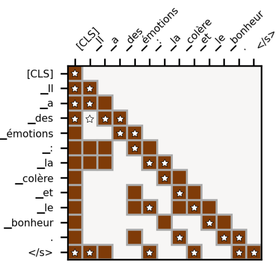
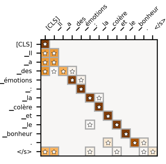
Figure 3: Learned patterns by Sparsefinder $k$-means (left) and the subsequent attention weights (right). Starred blocks represent ground-truth edges.

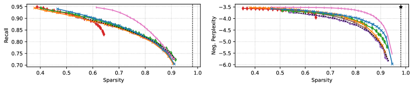
Figure 4: Sparsity-recall and sparsity-(neg-)perplexity tradeoff averaged across all layers and heads on WikiText-103. The vertical dashed line represents the gold sparsity obtained by the full $\alpha$-entmax transformer.

6 Experiments: Masked LM

Setup.

Following Beltagy et al. (2020), we initialize our model from a pretrained RoBERTa checkpoint. We use the roberta-base model from Huggingface’s transformers library, with 12 layers and 12 heads. We finetune on WikiText-103 (Merity et al., 2017), replacing softmax by $\alpha\text{-entmax}$ with $\alpha=1.5$ for all heads. Training details, model hyperparameters, and data statistics can be found in §D.

Learning projections.

As done for MT experiments, we learn to project keys and queries from the original 64 dimensions into $r=4$ dimensions. To this end, we use 1K random samples from the training set, each with length of 512, keeping half for validation. We extract the $\alpha\text{-entmax}$ attention graphs $\mathcal{G}_{h}$ but from the encoder self-attention of each head, leading to an average of 3M positive pairs per layer. Due to the small number of learnable parameters for each head ($256$), training was done with Adam for one epoch.

Results.

Our full transformer trained with $\alpha$-entmax achieved a perplexity score of $3.5004$ with an overall sparsity of $0.9804$ on WikiText-103. As in sentence-level MT experiments, we measure the sparsity-recall and the sparsity-perplexity tradeoff via the change of $\mathcal{G}_{h}$ with $\hat{\mathcal{G}}_{h}$ at test time. Moreover, since MLM has longer inputs, we increased the range of the window pattern to $\{31,41,51,75,101,125,151,175,201,251\}$.

We show in Figure 4 the Pareto curves for the tradeoff between sparsity and recall (left), and the tradeoff between sparsity and perplexity (right). The curves for the sparsity-recall tradeoff are similar to the ones found in MT experiments, with the distance-based method outperforming all methods, followed by the $k$-means variant of Sparsefinder and Routing Transformer. In terms of perplexity, our distance-based approach also Pareto-dominates other methods, followed by our clustering variant and Routing Transformer. As in the MT experiments, the window baseline yields a similar sparsity-recall curve to other approaches, reinforcing the importance of local patterns. Although the distance-based method requires a quadratic number of computations, it reduces them by a factor of $d/r=64/4=16$, as described in §4.3, and achieves better recall and perplexity than any other tested method. This finding indicates clear room for improvement in designing efficient attention methods that have a better tradeoff between efficiency and accuracy than existing approaches.

Learned patterns.

In Figure 5 we show Sparsefinder $k$-means’ predicted attention graphs for a specific attention head that originally learned to focus on coreference tokens. We can see that the pattern induced by Sparsefinder keeps the behavior of attending to coreferences. Concretely, our method achieves a high recall score ($\sim 80\%$) with a high sparsity rate ($\sim 75\%$) on this attention head.

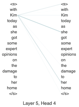
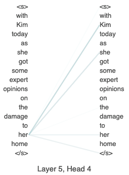
Figure 5: Attention pattern learned by Sparsefinder $k$-means that focus on coreference tokens.

Cluster analysis.

To understand what is represented in each cluster learned by Sparsefinder $k$-means, we run the following experiment: we obtain POS tags using spaCy, and calculate the distribution of each tag over clusters for all heads. We show an example in Figure 6, where Sparsefinder learned a cluster that makes verbs and nouns attend to themselves, and additionally to most auxiliary verbs.

Figure 6: Percentage of POS tags assigned to a given cluster on the entire Wikitext 103 validation set.

6.1 Efficient Sparsefinder

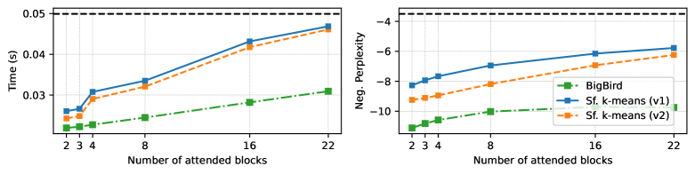
Figure 7: Comparison of Sparsefinder and BigBird in terms of running time and (negative) perplexity by varying the number of attended blocks. The black dashed line represents the results obtained by the full $\alpha$-entmax transformer.

We now turn to the question of making Sparsefinder efficient in practice. Before we proceed, we note that comparison between methods usually depends on the specific implementation used, which influences the measurements and can also require specialized hardware. This leaves BigBird and Routing Transformer as the only models we can compare with in practice: Reformer includes other optimizations that are not part of the attention mechanism, and Longformer is based on CUDA kernels, specialized for fast computation. Lastly, the strategy used in Routing Transformer is incorporated in Sparsefinder (v2), where we use Sparsefinder’s centroids with Routing Transformer top-$k$ strategy. In order to make Sparsefinder more efficient, we adopt the key strategy of BigBird: work with contiguous chunks rather than single tokens, creating blocks in the attention matrix. More precisely, we learn projections over chunked tokens following Equation 7, where $(\mathbf{q}^{\prime},\mathbf{k}^{\prime}_{P})$ is a positive pair if any token inside the chunk is part of a positive pair of the original $\alpha$-entmax graph, and similarly, a pair $(\mathbf{q}^{\prime},\mathbf{k}^{\prime}_{N})$ is negative if all tokens inside the chunk are negative. Thus, given a block/chunk size $z$, the size of the dense attention graph reduces from $|\mathcal{G}_{h}|=nm$ to $|\mathcal{G}_{h}|=\lceil nm/z^{2}\rceil$ (with zero-padding).

Implementation.

In order to be comparable to BigBird, we implement a routine that caps the maximum number of attended blocks in Sparsefinder, analogous to the number of random blocks used in BigBird. We propose two variants: (v1) computes dot-products between all chunked vector projections and then returns the top-$k$ blocks, and (v2) selects the top-$k$ blocks closest to the learned centroids and computes dot-products for these blocks. The first variant is more costly, yet it may lead to a more robust selection, whereas the second variant resembles Routing Transformer’s top-$k$ strategy.

Results.

We measure the clock-time of the MLM model evaluated on 500 examples with a batch size of 8. We vary the number of attended blocks within {2, 3, 4, 8, 16, 22 $\approx\sqrt{n}$}, the block size in {2, 4, 8, 16}, and compute perplexity for values of $B$ (number of clusters) within {2, 4, 8, 12, 16, 20}. We use a window size of $3$ in all experiments to capture the controlled hyperparameters’ impact better. Figure 7 shows plots by averaging runs with different block sizes and number of clusters. As expected, using a lower number of attended blocks leads to improvements in terms of running time, yet all models perform poorly on the MLM task. As we increase the number of blocks, we can see both a boost in terms of MLM performance and an increased running time. By comparing Sparsefinder and BigBird, we notice that BigBird is faster than Sparsefinder, but increasing the number of attended (random) blocks in BigBird does not lead to significant improvements on the real task. In contrast, both versions of Sparsefinder can improve the MLM performance while still being faster than a regular $\alpha$-entmax transformer. In particular, by attending to only 2 blocks, Sparsefinder is able to achieve a better MLM score than BigBird with 22 random blocks while still being faster than it. Plots for each block size can be found in §F.

7 Conclusions

We proposed Sparsefinder, a method to identify the sparsity pattern of entmax-based transformers while avoiding full computation of the score matrix. Our method learns a low-dimensional projection of queries and keys with a contrastive objective, and comes with three variants: distance, quantization, and clustering-based. We compared these variants against competing approaches on two tasks: machine translation and masked language modeling. We obtained favorable sparsity-recall and sparsity-accuracy tradeoff curves. Our theoretical sparsity provides a lower bound for how much computational sparsity can be achieved, and may guide future research on efficient transformers. Finally, we proposed a simple extension of Sparsefinder that resembles the block-based attention of BigBird by learning projections of chunked tokens, which exhibits a promising direction in terms of the trade-off of learnable sparsity with computation time and accuracy.

Appendix A Sparse Attention

A natural way to get a sparse attention distribution is by using the sparsemax transformation (Martins and Astudillo, 2016), which computes an Euclidean projection of the score vector onto the probability simplex $\triangle^{n}:=\{\mathbf{p}\in\mathbb{R}^{n}\mid\mathbf{p}\geq\mathbf{0},\,\,\mathbf{1}^{\top}\mathbf{p}=1\}$, or, more generally, the $\alpha$-entmax transformation (Peters et al., 2019):

$$\alpha\text{-entmax}(\mathbf{z}):=\operatorname*{\text{arg\,max}}_{\mathbf{p}\in\triangle^{n}}\mathbf{p}^{\top}\mathbf{z}+H_{\alpha}(\mathbf{p}),$$ (10)

where $H_{\alpha}$ is a generalization of the Shannon and Gini entropies proposed by Tsallis (1988), parametrized by a scalar $\alpha\geq 1$:

$$H_{\alpha}(\mathbf{p}):=\begin{cases}\frac{1}{\alpha(\alpha-1)}\sum_{j}(p_{j}-p_{j}^{\alpha}),&\alpha\neq 1\\ -\sum_{j}p_{j}\log p_{j},&\alpha=1.\end{cases}$$ (11)

Setting $\alpha=1$ recovers the softmax function, while for any value of $\alpha>1$ this transformation can return a sparse probability vector. Letting $\alpha=2$, we recover sparsemax. A popular choice is $\alpha=1.5$, which has been successfully used in machine translation and morphological inflection applications (Peters et al., 2019; Correia et al., 2019).

Proof to Proposition 1.

Proof.

From the definition of $\mathbf{z}|_{\mathbf{m}}$ and from Eq. 2, we have that

$$\begin{cases}z_{j}|_{\mathbf{m}}=z_{j}>\frac{\tau(\mathbf{z})}{\alpha-1}&\text{if }p_{j}^{*}>0\\ z_{j}|_{\mathbf{m}}\leq z_{j}\leq\frac{\tau(\mathbf{z})}{\alpha-1}&\text{if }p_{j}^{*}=0.\end{cases}$$ (12)

We first prove that $\tau(\mathbf{z}|_{\mathbf{m}})=\tau(\mathbf{z})$. From the definition of $\tau(\mathbf{z})$ we have that $\sum_{j}[(\alpha-1)z_{j}-\tau(\mathbf{z})]_{+}^{\nicefrac{{1}}{{\alpha-1}}}=1$. Plugging the (in)equalities from Eq. 12, we thus have

$$1 =\sum_{j}[(\alpha-1)z_{j}-\tau(\mathbf{z})]_{+}^{\nicefrac{{1}}{{\alpha-1}}}=\sum_{j}[(\alpha-1)z_{j}|_{\mathbf{m}}-\tau(\mathbf{z})]_{+}^{\nicefrac{{1}}{{\alpha-1}}}.$$ (13)

Since $\tau(\mathbf{z})$ satisfies the second equation – which is the condition that defines $\tau(\mathbf{z}|_{\mathbf{m}})$ – we thus conclude that $\tau(\mathbf{z}|_{\mathbf{m}})=\tau(\mathbf{z})$. Combining the results in Eqs. 12–13, we see that the supports of $\alpha\text{-entmax}(\mathbf{z})$ and $\alpha\text{-entmax}(\mathbf{z}|_{\mathbf{m}})$ are the same and so are the thresholds $\tau$, and therefore from Eq. 2 we conclude that $\alpha\text{-entmax}(\mathbf{z}|_{\mathbf{m}})=\alpha\text{-entmax}(\mathbf{z})$. ∎

Appendix B Computing infrastructure

Our infrastructure consists of 4 machines with the specifications shown in Table 1. The machines were used interchangeably, and all experiments were executed in a single GPU. Despite having machines with different specifications, we did not observe large differences in the execution time of our models across different machines.

#	GPU	CPU
1.	4 $\times$ Titan Xp - 12GB	16 $\times$ AMD Ryzen 1950X @ 3.40GHz - 128GB
2.	4 $\times$ GTX 1080 Ti - 12GB	8 $\times$ Intel i7-9800X @ 3.80GHz - 128GB
3.	3 $\times$ RTX 2080 Ti - 12GB	12 $\times$ AMD Ryzen 2920X @ 3.50GHz - 128GB
4.	3 $\times$ RTX 2080 Ti - 12GB	12 $\times$ AMD Ryzen 2920X @ 3.50GHz - 128GB

Table 1: Computing infrastructure.

Appendix C Machine Translation

C.1 Setup

Data.

Statistics for all datasets used in MT experiments can be found below in Table 2.

Dataset	# train	# test	Avg. sentence length
IWSLT17 (en$\to$de)	206K	1080	20 ±14    /    19 ±13
IWSLT17 (en$\to$fr)	233K	1210	20 ±14    /    21 ±15

Table 2: Statistics for MT datasets.

Training and Model.

We replicated the sentence-level model of Fernandes et al. (2021) with the exception that we used $\alpha$-entmax with $\alpha=1.5$ instead of softmax in all attention heads and layers. Table 3 shows some architecture (transformer large) and training hyperparameters used for MT experiments. We refer to the original work of Fernandes et al. (2021) for more training details.

Hyperparam.	Value
Hidden size	1024
Feedforward size	4096
Number of layers	6
Number of heads	16
Attention mapping $\pi$	$1.5$-entmax
Optimizer	Adam
Number of epochs	20
Early stopping patience	10
Learning rate	0.0005
Scheduling	Inverse square root
Linear warm-up steps	4000
Dropout	0.3
CoWord dropout	0.1
Beam size	5

Table 3: Hyperparmeters for neural machine translation models.

C.2 Projections setup

Data.

Statistics for the subsets of IWSLT used in the projection analysis can be found below in Table 4.

	Train				Validation
Pair	# sent.	# pos. pairs	Avg. sent. length		# sent.	# pos. pairs	Avg. sent. length
en$\to$de	9K	8M ±1M	35 ±16		1K	330K ±56K	36 ±17
en$\to$fr	9K	9M ±1M	37 ±17		1K	334K ±58K	37 ±16

Table 4: Statistics for subsets of IWSLT used for training and evaluating projections.

Training.

After extracting the $\alpha$-entmax graphs, we optimize the learnable parameters of Equation 7 with Adam over a single epoch. Moreover, we used the $k$-means implementation from scikit-learn (Pedregosa et al., 2011) for our clustering-based approach. The hyperparameters used both for training the projections and for clustering with $k$-means are shown in Table 5.

Hyperparam.	Value
Projection dim. $r$	4
Loss margin $\omega$	1.0
Batch size	16
Optimizer	Adam
Number of epochs	1
Learning rate	0.01
$\ell_{2}$ regularization	0
$k$-means init	$k$-means++
$k$-means max num. inits	10
$k$-means max iters	300

Table 5: Hyperparmeters for MT projections.

Projection analysis.

We compare Sparsefinder, varying $B\in\{2,4,6,8,10,12\}$ for bucket-based methods, and $t\in\{0.5,1.0,1.5,2.0,2.5\}$ for the distance-based variant, with the following methods:

• Window baseline: connect all query and key pairs within a sliding window of size $w\in\{0,1,3,5,7,9,11,15,19,23,27\}$.

• Learnable patterns: Reformer by varying the number of buckets within $\{2,4,6,8,10,12\}$; Routing transformer by varying the number of clusters within $c\in\{2,4,6,8,10\}$ with top-$k$ set to $\lceil n/c\rceil$ (i.e. balanced clusters).

• Fixed patterns: BigBird by varying the number of random blocks within $\{2,4,6,8,10\}$ with a block size of $1$; Longformer by varying the number of random global tokens within $\{4,8,12,16,20\}$.

Sparsity-recall tradeoff per layer and head.

Plots are shown in Figures 8 and 9 for en$\to$de and en$\to$fr, respectively.

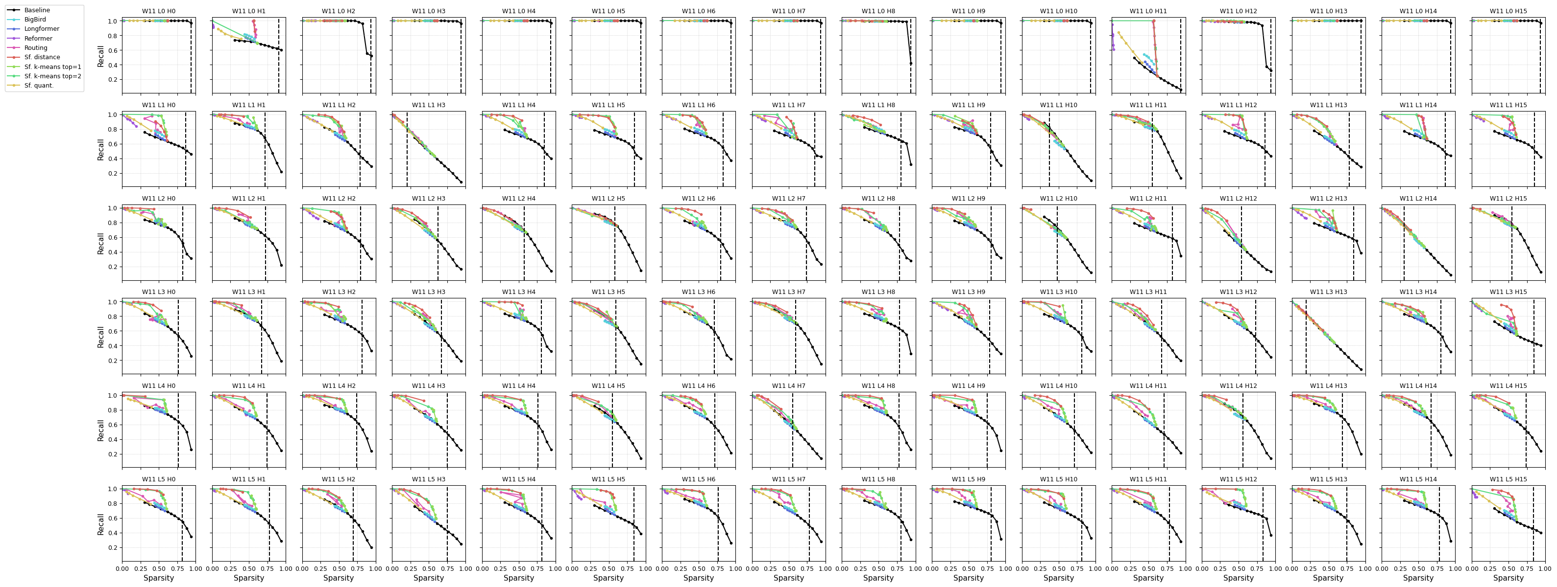
Figure 8: Sparsity-recall tradeoffs with a fixed window pattern of size 11 for en$\to$de.

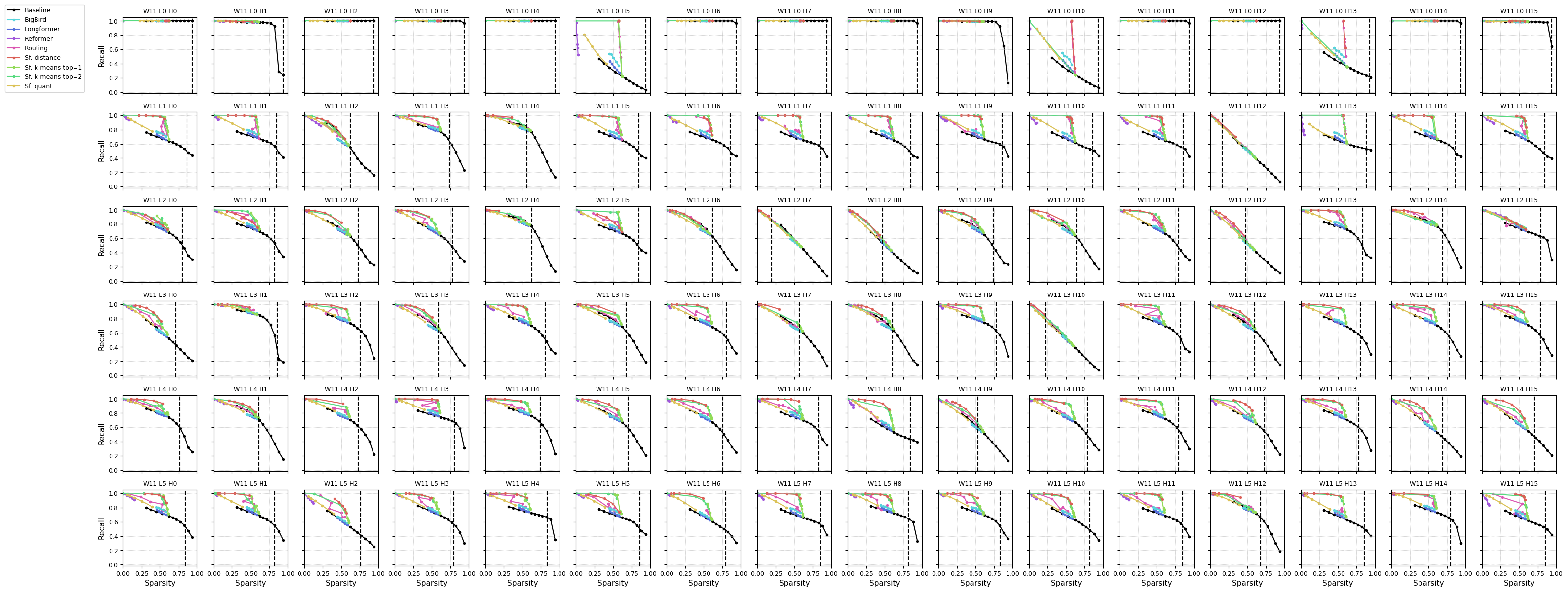
Figure 9: Sparsity-recall tradeoffs with a fixed window pattern of size 11 for en$\to$fr.

Appendix D Masked Language Modeling

D.1 Setup

Data and model.

In order to have a transformer model trained with $\alpha$-entmax, we finetuned RoBERTa-Base (Liu et al., 2019) on WikiText-103 (Merity et al., 2017) over 3000 steps with Adam (learning rate of $3\times 10^{-5}$). To mimic the finetuning approach adopted by Longformer, we employed a batch size of 2 by accumulating gradients over 32 steps due to GPU memory constraints. Table 6 shows some architecture (transformer large) and training hyperparameters used for MT experiments. We refer to the original work of Liu et al. (2019) for more architecture details.

Hyperparam.	Value
Hidden size	64
Feedforward size	3072
Max input length	514
Number of layers	12
Number of heads	12
Attention mapping $\pi$	$1.5$-entmax
Optimizer	Adam
Number of steps	3000
Learning rate	0.00003

Table 6: Hyperparmeters for masked language modeling models.

D.2 Projections setup

Data and training.

The subset used for Masked LM projections experiments contains 500 instances for training and 500 instances for validation. Moreover, all instances have a sentence length of 512 tokens. We got 3M (±1M) positive pairs for training and 2.5M (±1M) for validation. The hyperparameters for Masked LM are the same as the ones used in the MT experiments, shown in Table 5.

Projection analysis.

We perform the same analysis as in MT, but now we vary the window size of the baseline within {0, 1, 3, 7, 11, 25, 31, 41, 51, 75, 101, 125, 151, 175, 201, 251, 301, 351, 401, 451, 501, 512}.

Sparsity-recall tradeoff per layer and head.

Plots are shown next in Figure 10.

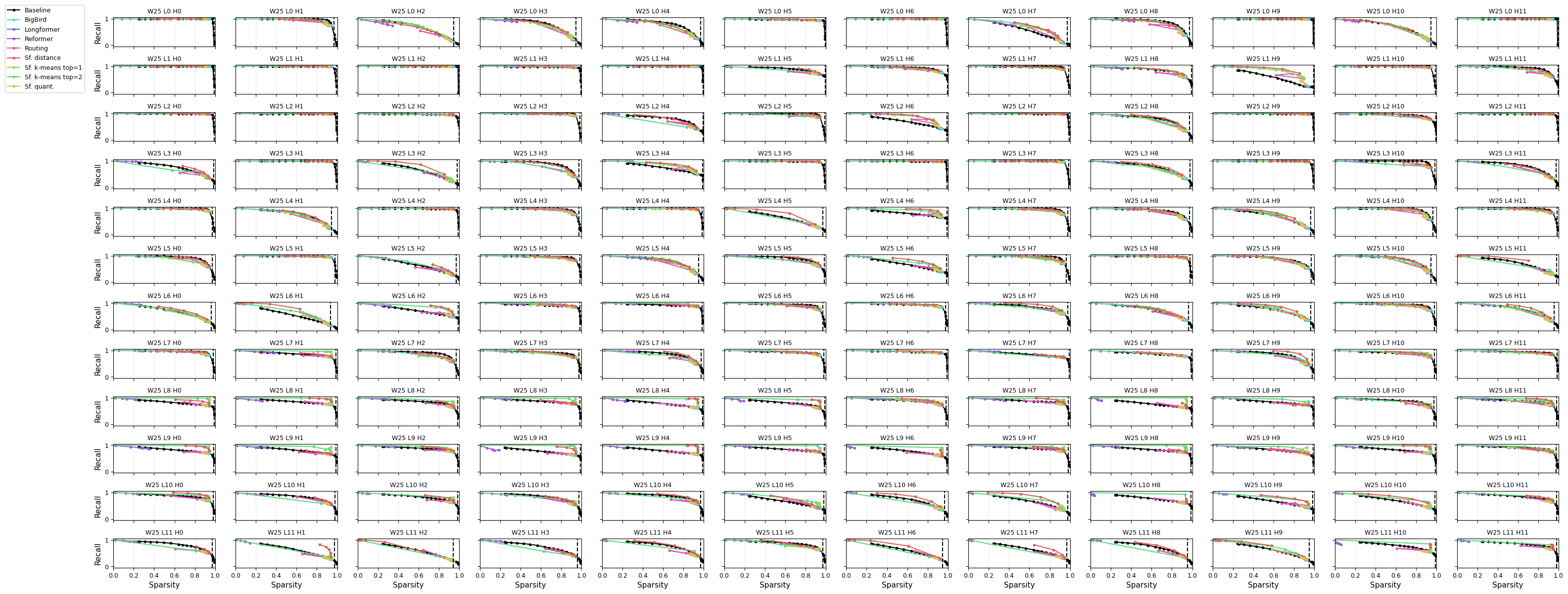
Figure 10: Sparsity-recall tradeoffs with a fixed window pattern of size 25 for MLM.

Appendix E Attention plots

Examples of attention maps can be seen in Figure 11 and 12.

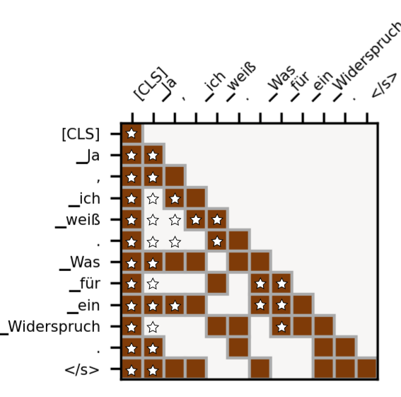
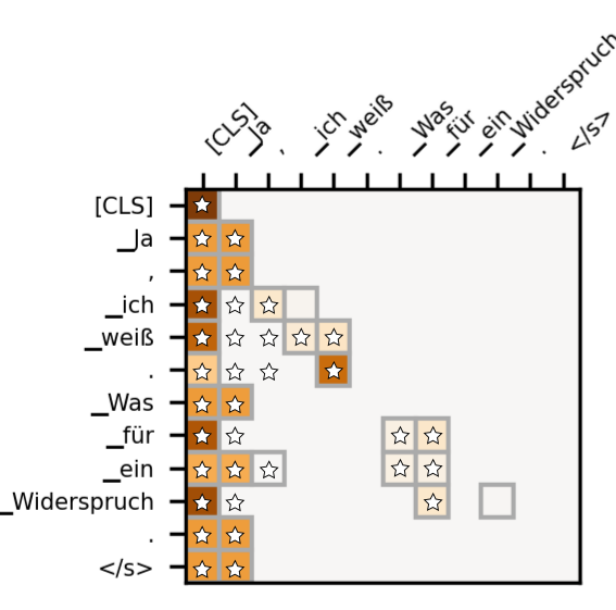
Figure 11: Learned patterns by Sparsefinder $k$-means (left) and the subsequent attention weights (right). Starred blocks represent ground-truth edges.

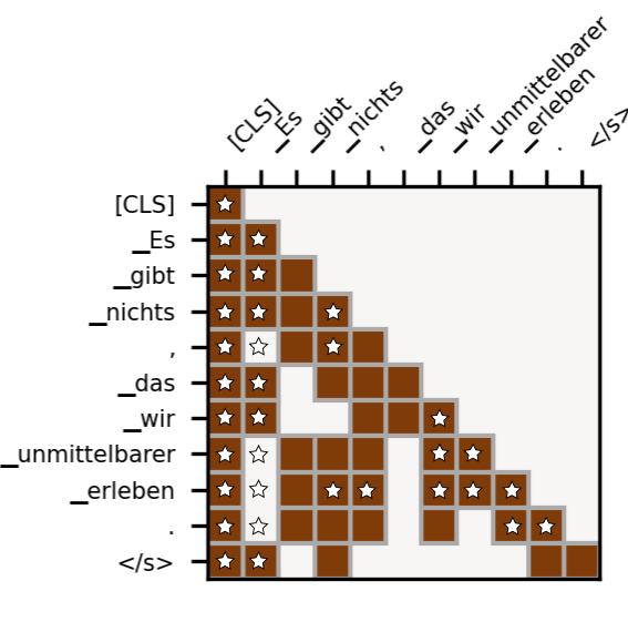
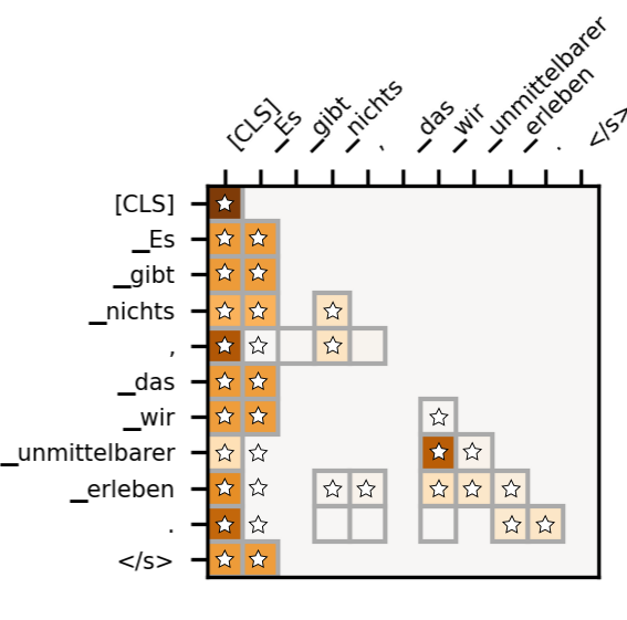
Figure 12: Learned patterns by Sparsefinder $k$-means (left) and the subsequent attention weights (right). Starred blocks represent ground-truth edges.

Appendix F Efficient Sparsefinder

Plots for block size within {1,2,4,8,16} are shown in 13. For these experiments, we used a window size of 3 for all methods in order to better measure the impact of others hyper-parameters.

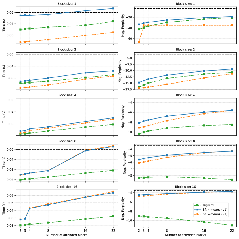
Figure 13: Comparison between Sparsefinder and BigBird in terms of running time and (negative) perplexity as a function of the number of random blocks for several block sizes. The horizontal dashed line represents the results obtained by the full $\alpha$-entmax transformer.

References

- Bellet et al. (2015) Aurélien Bellet, Amaury Habrard, and Marc Sebban. 2015. Metric learning. Synthesis Lectures on Artificial Intelligence and Machine Learning, 9(1):1–151.
- Beltagy et al. (2020) Iz Beltagy, Matthew E. Peters, and Arman Cohan. 2020. Longformer: The long-document transformer. arXiv:2004.05150.
- Brown et al. (2020) Tom B Brown, Benjamin Mann, Nick Ryder, Melanie Subbiah, Jared Kaplan, Prafulla Dhariwal, Arvind Neelakantan, Pranav Shyam, Girish Sastry, Amanda Askell, et al. 2020. Language models are few-shot learners. In Advances in Neural Information Processing Systems (NeurIPS), volume 33, pages 1877–1901. Curran Associates, Inc.
- Cettolo et al. (2017) Mauro Cettolo, Marcello Federico, Luisa Bentivogli, Niehues Jan, Stüker Sebastian, Sudoh Katsuitho, Yoshino Koichiro, and Federmann Christian. 2017. Overview of the iwslt 2017 evaluation campaign. In Proceedings of the 14th International Workshop on Spoken Language Translation (IWSLT), pages 2–14.
- Child et al. (2019) Rewon Child, Scott Gray, Alec Radford, and Ilya Sutskever. 2019. Generating long sequences with sparse transformers. arXiv preprint arXiv:1904.10509.
- Choromanski et al. (2021) Krzysztof Marcin Choromanski, Valerii Likhosherstov, David Dohan, Xingyou Song, Andreea Gane, Tamas Sarlos, Peter Hawkins, Jared Quincy Davis, Afroz Mohiuddin, Lukasz Kaiser, David Benjamin Belanger, Lucy J Colwell, and Adrian Weller. 2021. Rethinking attention with performers. In International Conference on Learning Representations (ICLR).
- Correia et al. (2019) Gonçalo M. Correia, Vlad Niculae, and André F. T. Martins. 2019. Adaptively sparse transformers. In Proceedings of the 2019 Conference on Empirical Methods in Natural Language Processing and the 9th International Joint Conference on Natural Language Processing (EMNLP-IJCNLP), pages 2174–2184, Hong Kong, China. Association for Computational Linguistics.
- Daras et al. (2020) Giannis Daras, Nikita Kitaev, Augustus Odena, and Alexandros G Dimakis. 2020. Smyrf - efficient attention using asymmetric clustering. In Advances in Neural Information Processing Systems, volume 33, pages 6476–6489. Curran Associates, Inc.
- de Amorim (2012) Renato Cordeiro de Amorim. 2012. Constrained clustering with minkowski weighted k-means. In 2012 IEEE 13th International Symposium on Computational Intelligence and Informatics (CINTI), pages 13–17. IEEE.
- Devlin et al. (2019) Jacob Devlin, Ming-Wei Chang, Kenton Lee, and Kristina Toutanova. 2019. BERT: Pre-training of deep bidirectional transformers for language understanding. In Proceedings of the 2019 Conference of the North American Chapter of the Association for Computational Linguistics: Human Language Technologies, Volume 1 (Long and Short Papers), pages 4171–4186, Minneapolis, Minnesota. Association for Computational Linguistics.
- Esplà et al. (2019) Miquel Esplà, Mikel Forcada, Gema Ramírez-Sánchez, and Hieu Hoang. 2019. ParaCrawl: Web-scale parallel corpora for the languages of the EU. In Proceedings of Machine Translation Summit XVII Volume 2: Translator, Project and User Tracks, pages 118–119, Dublin, Ireland. European Association for Machine Translation.
- Fernandes et al. (2021) Patrick Fernandes, Kayo Yin, Graham Neubig, and André F. T. Martins. 2021. Measuring and increasing context usage in context-aware machine translation. In Joint Conference of the 59th Annual Meeting of the Association for Computational Linguistics and the 11th International Joint Conference on Natural Language Processing (ACL-IJCNLP), Virtual.
- Katharopoulos et al. (2020) A. Katharopoulos, A. Vyas, N. Pappas, and F. Fleuret. 2020. Transformers are rnns: Fast autoregressive transformers with linear attention. In Proceedings of the International Conference on Machine Learning (ICML).
- Kitaev et al. (2019) Nikita Kitaev, Steven Cao, and Dan Klein. 2019. Multilingual constituency parsing with self-attention and pre-training. In Proceedings of the 57th Annual Meeting of the Association for Computational Linguistics, pages 3499–3505, Florence, Italy. Association for Computational Linguistics.
- Kitaev et al. (2020) Nikita Kitaev, Lukasz Kaiser, and Anselm Levskaya. 2020. Reformer: The efficient transformer. In International Conference on Learning Representations (ICLR).
- Liu et al. (2019) Yinhan Liu, Myle Ott, Naman Goyal, Jingfei Du, Mandar Joshi, Danqi Chen, Omer Levy, Mike Lewis, Luke Zettlemoyer, and Veselin Stoyanov. 2019. Roberta: A robustly optimized bert pretraining approach. arXiv preprint arXiv:1907.11692.
- Martins and Astudillo (2016) Andre Martins and Ramon Astudillo. 2016. From softmax to sparsemax: A sparse model of attention and multi-label classification. In International Conference on Machine Learning (ICML), volume 48 of Proceedings of Machine Learning Research, pages 1614–1623, New York, New York, USA. PMLR.
- Merity et al. (2017) Stephen Merity, Caiming Xiong, James Bradbury, and Richard Socher. 2017. Pointer sentinel mixture models. In 5th International Conference on Learning Representations (ICLR).
- Pedregosa et al. (2011) F. Pedregosa, G. Varoquaux, A. Gramfort, V. Michel, B. Thirion, O. Grisel, M. Blondel, P. Prettenhofer, R. Weiss, V. Dubourg, J. Vanderplas, A. Passos, D. Cournapeau, M. Brucher, M. Perrot, and E. Duchesnay. 2011. Scikit-learn: Machine learning in Python. Journal of Machine Learning Research (JMLR), 12:2825–2830.
- Peters et al. (2019) Ben Peters, Vlad Niculae, and André F. T. Martins. 2019. Sparse sequence-to-sequence models. In Proceedings of the 57th Annual Meeting of the Association for Computational Linguistics, pages 1504–1519, Florence, Italy. Association for Computational Linguistics.
- Post (2018) Matt Post. 2018. A call for clarity in reporting BLEU scores. In Proceedings of the Third Conference on Machine Translation: Research Papers, pages 186–191, Brussels, Belgium. Association for Computational Linguistics.
- Raganato et al. (2020) Alessandro Raganato, Yves Scherrer, and Jörg Tiedemann. 2020. Fixed encoder self-attention patterns in transformer-based machine translation. In Findings of the Association for Computational Linguistics: EMNLP 2020, pages 556–568, Online. Association for Computational Linguistics.
- Raganato and Tiedemann (2018) Alessandro Raganato and Jörg Tiedemann. 2018. An analysis of encoder representations in transformer-based machine translation. In Proceedings of the 2018 EMNLP Workshop BlackboxNLP: Analyzing and Interpreting Neural Networks for NLP, pages 287–297, Brussels, Belgium. Association for Computational Linguistics.
- Roy et al. (2021) Aurko Roy, Mohammad Saffar, Ashish Vaswani, and David Grangier. 2021. Efficient content-based sparse attention with routing transformers. Transactions of the Association for Computational Linguistics (TACL), 9:53–68.
- Sennrich et al. (2016) Rico Sennrich, Barry Haddow, and Alexandra Birch. 2016. Neural machine translation of rare words with subword units. In Proceedings of the 54th Annual Meeting of the Association for Computational Linguistics (Volume 1: Long Papers), pages 1715–1725, Berlin, Germany. Association for Computational Linguistics.
- Sun et al. (2021) Simeng Sun, Kalpesh Krishna, Andrew Mattarella-Micke, and Mohit Iyyer. 2021. Do long-range language models actually use long-range context? In Proceedings of the 2021 Conference on Empirical Methods in Natural Language Processing, pages 807–822, Online and Punta Cana, Dominican Republic. Association for Computational Linguistics.
- Tay et al. (2020) Yi Tay, Dara Bahri, Liu Yang, Donald Metzler, and Da-Cheng Juan. 2020. Sparse sinkhorn attention. In International Conference on Machine Learning (ICML), pages 9438–9447. PMLR.
- Tsallis (1988) Constantino Tsallis. 1988. Possible generalization of boltzmann-gibbs statistics. Journal of Statistical Physics.
- Vaswani et al. (2017) Ashish Vaswani, Noam Shazeer, Niki Parmar, Jakob Uszkoreit, Llion Jones, Aidan N Gomez, Ł ukasz Kaiser, and Illia Polosukhin. 2017. Attention is all you need. In Advances in Neural Information Processing Systems (NeurIPS), volume 30, pages 5998–6008. Curran Associates, Inc.
- Voita et al. (2019) Elena Voita, David Talbot, Fedor Moiseev, Rico Sennrich, and Ivan Titov. 2019. Analyzing multi-head self-attention: Specialized heads do the heavy lifting, the rest can be pruned. In Proceedings of the 57th Annual Meeting of the Association for Computational Linguistics, pages 5797–5808, Florence, Italy. Association for Computational Linguistics.
- Vyas et al. (2020) A. Vyas, A. Katharopoulos, and F. Fleuret. 2020. Fast transformers with clustered attention. In Proceedings of the International Conference on Neural Information Processing Systems (NeurIPS).
- Wagstaff et al. (2001) Kiri Wagstaff, Claire Cardie, Seth Rogers, and Stefan Schrödl. 2001. Constrained k-means clustering with background knowledge. In International Conference on Machine Learning (ICML), page 577–584.
- Wang et al. (2021) Shuohang Wang, Luowei Zhou, Zhe Gan, Yen-Chun Chen, Yuwei Fang, Siqi Sun, Yu Cheng, and Jingjing Liu. 2021. Cluster-former: Clustering-based sparse transformer for question answering. In Findings of the Association for Computational Linguistics: ACL-IJCNLP 2021, pages 3958–3968, Online. Association for Computational Linguistics.
- Wang et al. (2020) Sinong Wang, Belinda Li, Madian Khabsa, Han Fang, and Hao Ma. 2020. Linformer: Self-attention with linear complexity. arXiv preprint arXiv:2006.04768.
- Weinberger and Saul (2009) Kilian Q Weinberger and Lawrence K Saul. 2009. Distance metric learning for large margin nearest neighbor classification. Journal of Machine Learning Research (JMLR), 10(2).
- Xing et al. (2002) Eric P Xing, Andrew Y Ng, Michael I Jordan, and Stuart Russell. 2002. Distance metric learning with application to clustering with side-information. In Advances in Neural Information Processing Systems (NeurIPS), volume 15, page 12.
- Zaheer et al. (2020) Manzil Zaheer, Guru Guruganesh, Kumar Avinava Dubey, Joshua Ainslie, Chris Alberti, Santiago Ontanon, Philip Pham, Anirudh Ravula, Qifan Wang, Li Yang, et al. 2020. Big bird: Transformers for longer sequences. Advances in Neural Information Processing Systems (NeurIPS), 33.
- Zhang et al. (2021) Biao Zhang, Ivan Titov, and Rico Sennrich. 2021. Sparse attention with linear units. arXiv preprint arXiv:2104.07012.
- Zhao et al. (2019) Guangxiang Zhao, Junyang Lin, Zhiyuan Zhang, Xuancheng Ren, Qi Su, and Xu Sun. 2019. Explicit sparse transformer: Concentrated attention through explicit selection. arXiv preprint arXiv:1912.11637.