Hypercubes of AGN Tori (HYPERCAT) – II. Resolving the Torus with Extremely Large Telescopes

Abstract

Recent infrared interferometric observations revealed sub-parsec scale dust distributions around active galactic nuclei (AGNs). Using images of Clumpy torus models and NGC 1068 as an example, we demonstrate that the near- and mid-infrared nuclear emission of some nearby AGNs will be resolvable in direct imaging with the next generation of 30 m telescopes, potentially breaking degeneracies from previous studies that used integrated spectral energy distributions of unresolved AGN tori. To that effect we model wavelength-dependent point spread functions from the pupil images of various telescopes: James Webb Space Telescope, Keck, Giant Magellan Telescope, Thirty Meter Telescope, and Extremely Large Telescope. We take into account detector pixel scales and noise, and apply deconvolution techniques for image recovery. We also model 2D maps of the 10-$\mu{\rm m}$ silicate feature strength, $S_{\!10}$, of NGC 1068 and compare with observations. When the torus is resolved, we find $S_{\!10}$ variations across the image. However, to reproduce the $S_{\!10}$ measurements of an unresolved torus a dusty screen of $A_{V}>9$ mag is required. We also fit the first resolved image of the K-band emission in NGC 1068 recently published by the GRAVITY collaboration, deriving likely model parameters of the underlying dust distribution. We find that both 1) an elongated structure suggestive of a highly inclined emission ring, and 2) a geometrically thin but optically thick flared disk where the emission arises from a narrow strip of hot cloud surface layers on the far inner side of the torus funnel, can explain the observations.

1 Introduction

The thermal emission from the central region of an active galactic nucleus (AGN) depends spectrally and spatially on the distribution of dust close to the accreting black hole. A central dusty “torus” unifies disparate AGN classes (Krolik & Begelman, 1988; Antonucci, 1993; Urry & Padovani, 1995), and more specifically, a toroidal distribution of clouds generally accounts for characteristic observed features (e.g., Nenkova et al., 2002, 2008a, 2008b; Hönig et al., 2006; Schartmann et al., 2008).

The central AGN tori are relatively small in the near-infrared (NIR) and mid-infrared (MIR), on scales of a few parsecs (e.g., Jaffe et al., 2004; Nenkova et al., 2008b; Ramos Almeida et al., 2011; Tristram et al., 2014), so not currently resolvable in direct images. For nearby AGNs the only spatially resolved observations of the inner few parsec come from interferometers such as VLTI/GRAVITY and VLTI/MIDI in NIR and MIR, and the Atacama Large Millimeter / submillimeter Array (ALMA) in the submillimeter regime. Especially in the IR the baseline coverage is comparatively poor, with just two to four telescopes sampling the Fourier space of spatial frequencies. Image reconstruction is either impossible, or relies heavily on modeling of the sampled brightness distribution. However, 2D images, as opposed to 1D visibilities or 1D spectral energy distributions (SED), are needed to break possible degeneracies in the IR radiative transfer (Vinković et al., 2003). The upcoming generation of extremely large telescopes (Giant Magellan Telescope, GMT; Thirty Meter Telescope, TMT; and Extremely Large Telescope, ELT) all have the potential of resolving the IR emission in nearby AGNs with their single-aperture mirrors (we use “single-dish” in the text for simplicity, but all these telescopes have either segmented mirrors or comprise several circular mirrors arranged in a fixed pattern).

Perhaps surprisingly, at mid-IR wavelengths “polar” emission is frequently observed (e.g., Hönig et al., 2012, 2013; Burtscher et al., 2013; López-Gonzaga et al., 2016; Leftley et al., 2018), extending perpendicular to the equatorial axis of the obscuring torus. Using simulations we can make progress to determine whether the torus produces this emission, or if additional material is required. The picture is complicated by the fact that the near- to mid-IR emission morphology does not necessarily follow the 3D dust distribution (see results in Nikutta et al. (2021, henceforth Paper I)). Motivated by the situation above, in Paper I we have demonstrated that the polar elongation could be reproduced under specific conditions by utilizing the set of Clumpy model images and dust maps together with the accompanying Hypercat software.

While we perform all analyses in this paper using the AGN torus models produced by Clumpy, we note that in principle any other image-generating models could be used in conjunction with the Hypercat software. With the Clumpy models we hold several parameters fixed, e.g., the dust composition, grain size distribution, sublimation temperature, spectral shape of the illuminating source, and the functional prescription of the “softness” of the polar torus edge (we use a Gaussian form).

Other models might make different assumptions about the parameters, and about the geometry itself. For instance, Hönig & Kishimoto (2010) studied several dust chemical compositions and grain size distributions, and improved handling of the diffuse radiation field in the torus, to investigate their influence on the shape of spectral energy distributions. Siebenmorgen et al. (2015) introduced a two-phase medium and fluffy (rather than spherical) dust grains in their AGN torus model to explain the observed range of silicate feature strengths and wavelengths of the peak emission. Stalevski et al. (2016) varied several parameters of their own two-phase Monte Carlo model to investigate the relation between $\rm L_{torus}/L_{AGN}$ and the dust covering factor. Hönig & Kishimoto (2017) distributed the bulk of dusty clouds in their revised CAT3D model along the polar axis of the AGN system to help explain the observed polar elongation of the MIR emission in several nearby AGNs. Each such model (and others not mentioned here explicitly) is motivated by answering different open questions.

We also note that to smoothly interpolate images in several orthogonal dimensions (the free model parameters; seven in the case of Clumpy), the changes between model images from one set of parameter values to a neighboring set ought to be smooth. This is potentially a challenge for Monte Carlo based models if the cloud configuration between model realizations is allowed to change (i.e., if the cloud realization is randomized each time). While Clumpy eponymously simulates clumpy AGN tori, it differs from Monte Carlo models in that the model image resulting from its radiative transfer is by construction the mean of an infinite number of individual model realizations. Monte Carlo models of clumpy dust distributions that generate the cloud geometry anew for each realization could potentially overcome the challenge by averaging the output images of many realizations with identical parameter values; but that may prove too expensive regarding the required compute time. Models which employ smooth dust distributions by design, such as in, e.g., Fritz et al. (2006), could be used immediately with Hypercat, provided they were packaged in an appropriate $n$-dimensional hypercube.

Here we use Hypercat simulations to model the nearby ($D=14.4$ Mpc) and bright ($L_{\rm bol}=0.15-1.5\times 10^{45}\,{\rm erg\,s^{-1}}$) AGN NGC 1068. Fitting the well-populated SED (Lopez-Rodriguez et al., 2018, hereafter LR18) with models generated by Clumpy (Nenkova et al., 2008a, b) provides geometrical parameters of the dust distribution. We compute the wavelength-dependent point spread functions (PSF) of several current and future telescopes – James Webb Space Telescope (JWST); Keck; Giant Magellan Telescope (GMT); Thirty Meter Telescope (TMT); Extremely Large Telescope (ELT) – to simulate realistic single-dish observations and determine the resolvability of nearby AGNs. Our simulations also serve as predictions of the image observations from future facilities with higher spatial resolution. The 10-$\mu{\rm m}$ silicate feature provides a valuable diagnostic of the dust distribution, especially when observed using an integral field unit (IFU) for spatially and spectrally resolved image cubes, which we also simulate. Finally, we directly fit the recent 2.2-$\mu{\rm m}$ image of NGC 1068 released by the Gravity Collaboration et al. (2020, hereafter G20), deriving likely physical and geometrical parameters governing the source.

2 NGC 1068 Case Study

2.1 Torus Parameters

The type 2 Seyfert galaxy NGC 1068 has been extensively studied in the IR using single-dish (e.g., Mason et al., 2006; Ramos Almeida et al., 2011; Alonso-Herrero et al., 2011; Lira et al., 2013; Ichikawa et al., 2015) and interferometric (e.g., Jaffe et al., 2004; Raban et al., 2009; Burtscher et al., 2013; López-Gonzaga et al., 2014) observations. ALMA submillimeter observations have recently resolved the molecular torus in NGC 1068 and constrained its diameter to $\sim\!\!12$ pc using the dust continuum at 432 $\mu{\rm m}$ and CO J=6-5 (García-Burillo et al., 2016), and then found a size $13\times 4$ pc in the HCN J=2-1 transition and $12\times 5$ pc for HCO⁺ J=3-2 (Imanishi et al., 2018). The torus is found to be inclined, and lopsided, at a position angle of its mid-plane about 100–110° east of north. Including the 432 $\mu{\rm m}$ dust continuum observations by ALMA as a constraint in the 1–432 $\mu{\rm m}$ nuclear SED fits of NGC 1068, Lopez-Rodriguez et al. (2018, hereafter LR18) derived the Clumpy torus parameters that best reproduced the observations. We adopt these model parameters for our present study; they are listed in Table 1. The position angle of the torus large axis in the plane of the sky, ${\rm PA}$$\sim$138° east of north, was taken from 2 $\mu{\rm m}$ polarimetric observations of the nucleus (Packham et al., 1997; Simpson et al., 2002; Lopez-Rodriguez et al., 2015; Gratadour et al., 2015). The 2 $\mu{\rm m}$ polarization is thought to arise from the absorption of aligned dust grains in the torus of NGC 1068 where the measured polarization angle indicates the global orientation of the equatorial plane of the torus. This ${\rm PA}$ has been further confirmed by means of magnetically aligned dust grains across the resolved equatorial axis of the torus using ALMA polarimetric 860 $\mu{\rm m}$ observations (Lopez-Rodriguez et al., 2020).

Figure 1 shows the distribution of the thermal emission within the 1–432 $\mu{\rm m}$ wavelength range for a Clumpy model with parameters from Table 1. The morphology of the emission changes dramatically across the wavelength regimes as also shown in figure 5 in LR18. For details on emission morphology please see the companion paper (Nikutta et al., 2021, henceforth Paper I).

Table 1: Clumpy Parameters and Derived Quantities from the Best-fit SED Model to NGC 1068 by LR18.

Model Parameters			Derived & Literature Values
$\sigma$ (deg)	$43^{+12}_{-15}$		$R_{\rm in}$ (pc)	$0.28^{+0.01}_{-0.01}$
$Y$	$18^{+1}_{-1}$		$R_{\rm out}$ (pc)	$5.1^{+0.4}_{-0.4}$
${\cal N}_{0}$	$4^{+2}_{-1}$		$H$ (pc)	$3.5^{+1.0}_{-1.3}$
$q$	$0.08^{+0.19}_{-0.06}$		$L_{\rm bol}/10^{44}$ (erg s-1)	$5.02^{+0.15}_{-0.19}$
$\tau_{\rm V}$	$70^{+6}_{-14}$		$D^{a}$ (Mpc)	$14.4$
$i$ (deg)	$75^{+8}_{-4}$		${\rm PA}$ (deg)	$138$

Note. — ^aAt $D=14.4$ Mpc, 1″ = 70 pc, adopting H₀ = 73 km s^-1 Mpc^-1 (Bland-Hawthorn et al., 1997).

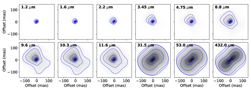
Figure 1: 2D torus thermal emission images of NGC 1068 modeled with Clumpy from 1.2 $\mu{\rm m}$ to 432 $\mu{\rm m}$ using the parameters from Table 1. The morphology varies as function of wavelength due to changes of optical depth and dust temperature. Blue contours show the fractional surface brightness at 0.05, 0.1, 0.3, 0.5, 0.7, and 0.9 of the peak value.

2.2 Single-dish Synthetic Observations of NGC 1068

2.2.1 Telescopes, Pupil Images and PSFs

To produce synthetic observations with a given telescope and instrument combination, the telescope PSF and the instrumental configuration are needed. A telescope PSF can be very complex (e.g., Krist et al., 2011; Perrin et al., 2012) and depends on many factors; for instance telescope aperture, telescope configuration, seeing conditions, adaptive optics configuration, and wavelength. Our aim is to provide the best-case scenario of a synthetic observation for a given telescope and wavelength. We assume perfect adaptive optics, and atmospheric conditions without sky or PSF variations. These conditions can be refined by applying specific aberrations relevant to the science cases and telescope/instrument configuration, but this is outside the scope of the present work. Future releases of Hypercat may incorporate tools to account for these conditions.

Table 2 summarizes the telescopes and instruments available in Hypercat, which include the next generation of 30 m telescopes (GMT, TMT, ELT) as well as JWST and Keck for comparison. For telescopes without an instrument in a given wavelength range the pixel scale is taken to be equal to the Nyquist sampling ($0.5\times\lambda/D$). The FWHM is given by $\lambda/D$, except for JWST, whose PSFs have been modeled in detail by the instrument teams.

Table 2: List of Single Dish Telescopes and Instruments Available with Hypercat.

Telescope	Diameter	Instrument	Wavelength	Pixel scale	FWHM
	(m)		($\mu{\rm m}$)	(mas)	(mas)
JWST	6.5	NIRCAM	0.6 - 5	31 - 63	31 - 162b
		NIRISS	0.6 - 5	31 - 63	42 - 152c
		MIRI	5 - 28	110	182 - 812d
Keck	10.0	NIRC2	0.9 - 5.3	10 - 40	163 - 241e
		Nyquista	8 - 20	83 - 206	165 - 412
GMT	24.5	GMTIFS	0.9 - 2.5	5	8 - 21
		Nyquista	3 - 5	12 - 21	25 - 42
		Nyquista	8 - 20	34 - 84	67 - 168
TMT	30.0	IRIS	0.85 - 2.5	4	6 - 17
		MICHI	3 - 5	11.9	21 - 34
		MICHI	8 - 12	27.5	55 - 82
ELT	39.1	MICADO	0.8 - 2.5	4	4 - 13
		METIS	2.9 - 5	4	15 - 26
		METIS	5 - 14	13	26 - 74

^aFor telescopes without an instrument in a given wavelength range, the pixel scale is set to the Nyquist sampling at the shortest wavelength. For FWHM values without a superscript, $\lambda/D$ was assumed. Otherwise the FWHM values are from:
^bhttps://jwst-docs.stsci.edu/near-infrared-camera/nircam-predicted-performance/nircam-point-spread-functions
^chttps://jwst-docs.stsci.edu/near-infrared-imager-and-slitless-spectrograph/niriss-predicted-performance/niriss-point-spread-functions
^dhttps://jwst-docs.stsci.edu/mid-infrared-instrument/miri-predicted-performance/miri-point-spread-functions
^ehttps://www2.keck.hawaii.edu/inst/nirc2/ScamCompare.html

We compute the PSF as the Fourier transform of the telescope pupil image (see Appendix A.1 for details). The PSF includes the effects of the telescope structures that interact with the science beam. The pupil images are in units of meters, which are then converted to arcsec using the PIXSCALE keyword in the corresponding FITS files. For any given wavelength and telescope, the PSF has a FWHM = $\lambda/D$. Figure 2 shows the pupils and PSFs of the telescopes from Table 2.

Note that Hypercat also provides two other methods to estimate the PSF: model-PSF, which is a combination of a central Airy disk that contains most of the power of the PSF, and a broad Gaussian halo that encompasses the remaining power of the object; and image-PSF where the user can provide as an image the empirical PSF of an observed standard star for a given telescope/instrument. model-PSF also accounts for Strehl ratio to perform studies of the AO system (Appendix A.1).

To qualitatively explore the PSF for each instrument at a given wavelength we produce monochromatic PSF images (Figure 2) at five representative wavelengths within the $1-13$ $\mu{\rm m}$ wavelength range for each of the telescopes in Table 2. Note that the throughput of a specific filter may be taken into account for a more realistic PSF. Here, the only diffractive and optical aberration component in our simulations comes from the pupil image.

Figure 3 shows the radial profiles (computed over circular annuli) of the PSFs of GMT, TMT, and ELT at 2.0 $\mu{\rm m}$. As expected, the ‘cleanest’ (most Airy-like) extended power of the PSF is provided by the GMT, while the highest-resolution core of the PSF is provided by the ELT. As shown by Angel et al. (2003), the best extended PSF will be provided by the telescope configuration with full disks, i.e., GMT, over those with fitted hexagons, i.e., ELT and TMT. This is because the extended regions of the PSF from fitted hexagons have more structures (i.e., ‘spider’ shape in the wings of the PSF) than those from full circular disks. The instrumental configuration will be thus of great importance when considering specific science goals of the ground-based 30 m class telescopes.

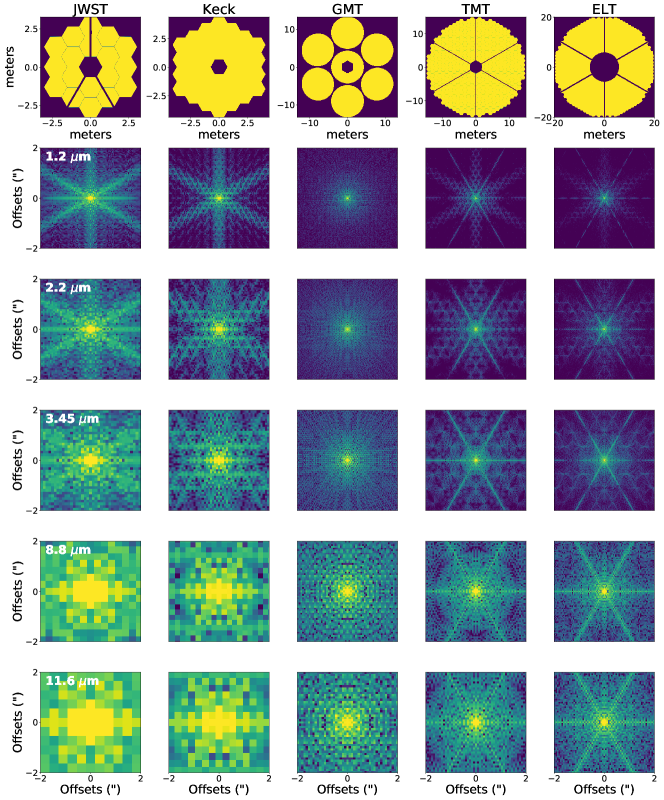
Figure 2: First row shows the pupil images of the JWST, Keck, GMT, TMT, and ELT from left to right. Their PSFs at 1.2, 2.2, 3.45, 8.8 and 11.6 $\mu{\rm m}$ within $4\times 4$ arcsec² from second to bottom row are shown in logarithmic scale. For all PSFs, we have adopted the Nyquist sampling as the pixel scale.

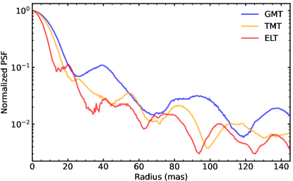
Figure 3: Radial profiles of the PSFs of GMT, TMT, and ELT within the central $\sim 145$ milliarcsec radius, at a wavelength of 2 $\mu{\rm m}$.

2.2.2 Toward a Synthetic Observation

Single-dish observations are degraded by several processes (Appendix A). The fundamental loss of resolution is due to convolution of the incoming wavefront with the PSF of the telescope. The PSF-convolved image is then downsampled to the discrete pixel sizes of the detectors. The PSF convolved and pixelated image (step E in Figure 4) is then flux calibrated. Specifically, the total flux of the model is equal to the flux density, in units of ’Jy’, from a known observation at the highest spatial resolution at a given wavelength. For our example, we used a flux density of 1 Jy at 3.45 $\mu$m by LR18. Finally, noise due to, for instance, fluctuations in detector readout, atmospheric emission and transmission is taken into account (Appendix A.4). Note that the final synthetic observations have a background set to zero, background subtraction is not required. Figure 4 shows this procedure using the 2D Clumpy torus image of NGC 1068 and the PSF of TMT at 3.45 $\mu{\rm m}$. These synthetic observations can be directly compared with real data. The rightmost column in Figure 4 shows the deconvolved images with and without noise. The improvement in detecting extended emission by deconvolving the noisy image is very conspicuous.

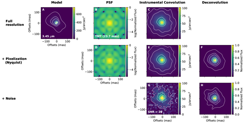
Figure 4: Hypercat step-by-step process to obtain synthetic observations from a 2D thermal emission map produced by using Clumpy models. From left to right the columns add operations on the input image by the optical system. From top to bottom the rows add detector degradations to the image. (A) 3.45 $\mu{\rm m}$ model image of NGC 1068 at full resolution (pixel scale 0.67 mas) using the parameters shown in Table 1, and applying a total flux density of 1.0 Jy obtained by LR18. All contours are shown at 0.01, 0.05, 0.1, 0.3, 0.5, 0.7, 0.9 fractions of the image peak. (B) PSF at 3.45 $\mu{\rm m}$ computed using the pupil image of TMT. The telescope angular resolution $\lambda/D=23.7$ mas is printed in the lower left corner. (C) Convolved image using the full resolution emission image (A) and PSF (B). (D) PSF pixelated at the Nyquist sampling of TMT at 3.45 $\mu{\rm m}$, i.e., $\lambda/D/2=11.87$ mas. Due to discretization limits (odd number of pixels is enforced by Hypercat), the effective pixel scale is 11.64 mas. (E) Convolved image of NGC 1068, pixelated at the same effective Nyquist sampling. (F) Deconvolved image using the pixelated image (E) and PSF (D). (G) Gaussian noise with SNR = 20 at the peak pixel was applied to the pixelated image of the thermal emission, E. (H) Deconvolved image using the pixelated PSF (D) and noisy image (G).

2.2.3 Results

Figure 5 shows the synthetic observations for each telescope in the 1.2-11.6 $\mu{\rm m}$ wavelength range. They were obtained following the steps shown in Figure 4 through step E, i.e., they are flux-calibrated and pixelated, but noise-free and not deconvolved.

An outstanding result is that all the upcoming generation of 30 m class telescopes will be able to spatially resolve the dust emission distribution of the torus around NGC 1068 in the $1-12$ $\mu{\rm m}$ wavelength range. Although the 6.5-m JWST telescope has the most sensitive capabilities, its resolving power, limited by the diameter of the telescope, is smaller than the torus size of NGC 1068 at any given wavelength in the IR. However, JWST can be used to isolate the torus emission from potential contributions of extended diffuse dust emission from the narrow line region (NLR), any polar/outflow components, and star-forming regions surrounding the AGN for a large sample of bolometric luminosities and AGN types. We also note that 10-m class telescopes, e.g., Keck, are not able to resolve the torus in NGC 1068 within the 1–12 $\mu{\rm m}$ wavelength range, in line with observations to date (e.g., Ramos Almeida et al., 2011; Alonso-Herrero et al., 2011; Asmus et al., 2015; Lopez-Rodriguez et al., 2016). We henceforth focus on the observations resolved by 30 m class telescopes.

In the 1–2.5 $\mu{\rm m}$ wavelength range the torus emission arises mostly from the directly irradiated clouds that make up the inner walls of the torus. In all cases, the region of emission is $<1$ pc (14 mas for NGC 1068) which is resolved by all 30 m class telescopes. Due to the shape of the PSF the extended torus emission is more clearly visible with GMT than with TMT or ELT. However, when deconvolution techniques are applied, TMT and ELT produce resolved images that are more comparable to the 2D original model images (see Figures 6 and 7)

In the 3–5 $\mu{\rm m}$ wavelength range the emission morphology becomes more extended, and importantly, the elongation is in the polar direction. If the torus axis is tilted with respect to the observer, the polar component is mainly seen on one side only due to self-obscuration by material in the equatorial region. The emission mainly originates from the inner layers of the extended dusty torus, and has sizes of $\sim$10 pc (142 mas), which are easily resolved by all 30 m class telescopes. For all these large telescopes the core and the extended emission are resolved. Deconvolution techniques can be applied effectively, and are crucial in providing final images comparable with the 2D models. These results demonstrate the criticality of obtaining not only an excellent but also stable PSF.

In the 8–12 $\mu{\rm m}$ wavelength range the torus emission shows an extended component in the polar direction, with a peak of emission in the northern inner wall of the torus. A small amount of emission is found along the equatorial plane of the torus due to the optically thick dust along such lines of sight. The extended emission is marginally resolved by all the 30 m class telescopes.

Apart from telescope size, instrument configuration and sensitivity, the physical/geometrical parameters of the AGN torus determine the resolvability of its emission. See Paper I on how these parameters affect resolvability and the existence of polar elongation of the emission across wavelengths.

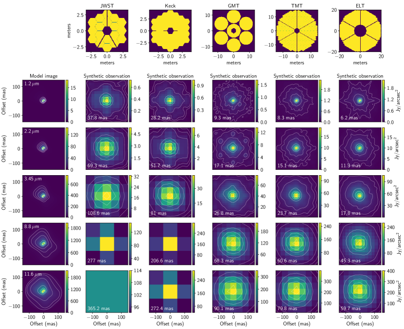
Figure 5: First row shows the pupil images of the JWST, Keck, GMT, TMT and ELT from left to right. From the second row, the first column shows the 2D Clumpy torus image of NGC 1068, and columns 2-6 show the synthetic observations for each telescope, for several wavelengths (rows 2-6). In all cases, model image and synthetic observations are flux calibrated and pixelated to Nyquist sampling. Contours are shown at levels of 0.03, 0.05, 0.1, 0.3, 0.5, 0.7, 0.9 times the peak of the image, except for the JWST and Keck at 8.8 and 11.6 $\mu$m because the pixelscale is similar to the FOV of the image. Each panel shows the angular resolution at the given wavelength estimated as $\lambda/D$.

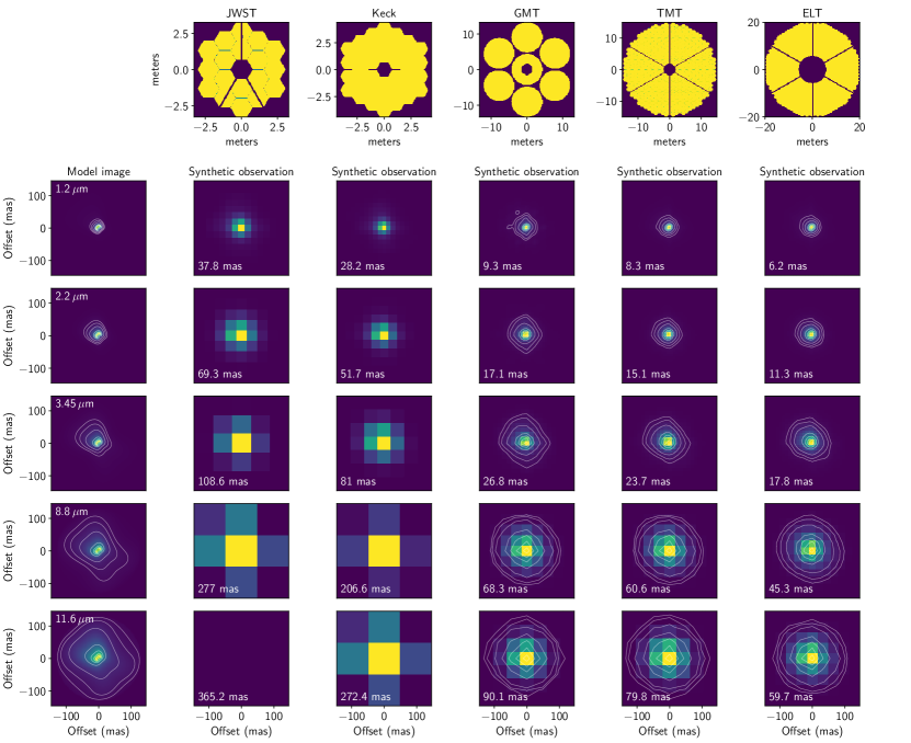
Figure 6: Deconvolved observations using pixelated images from Section A.5. First row and column as in Figure 5. The other panels show the deconvolved images as a function of wavelength and telescope. All panels were pixelated to the Nyquist sampling, and print in their lower-left corners the angular resolution at the given wavelength estimated as $\lambda/D$. Contours are shown at levels of 0.03, 0.05, 0.1, 0.3, 0.5, 0.7, 0.9 times the peak flux of the image. Contours for JWST and Keck are not shown because images are consistent with point sources at all wavelengths. The 11.6 $\mu$m image for the JWST is not visible because the pixel scale is similar to the FOV.

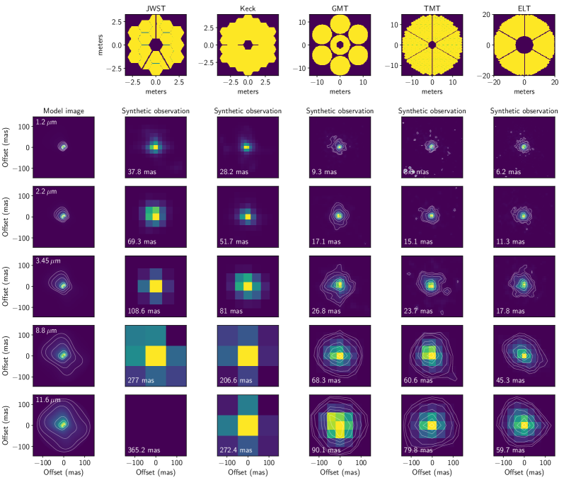
Figure 7: Deconvolved observations using noisy images from Section A.4. Same as Figure 6 but pixelated images with a SNR = 10 at the peak pixel have been deconvolved. Contours are shown at levels of 0.03, 0.05, 0.1, 0.3, 0.5, 0.7, and 0.9 times the peak of the image. Contours for JWST and Keck are not shown because images are consistent with point sources at all wavelengths. The 11.6 $\mu$m image for the JWST is not not visible because the pixel scale is similar to the FOV.

2.3 Spatially Resolved Spectral Features

Having the resolved images available at any wavelength, we can compute spectral quantities per-pixel, akin to observations with an Integral Field Unit (IFU). We demonstrate this with the 10 $\mu{\rm m}$ silicate feature strength $S_{\!10}$, defined as

$$S_{\!10}\ =\ln{\frac{F(\lambda_{10})}{F_{\rm cont}(\lambda_{10})}},$$ (1)

i.e., the logarithmic ratio of the flux at the extremum of the 10 $\mu{\rm m}$ feature and the continuum flux at that wavelength (interpolated as a cubic spline across the wings of the silicate feature; Spoon et al., 2007).

The silicates that make up the majority of ISM dust have stretching and bending modes which produce emission at 10 and 18 $\mu{\rm m}$. In the context of the AGN torus, the strength of the 10 $\mu{\rm m}$ feature is a powerful diagnostic because it is sensitive to several physical and geometrical conditions in the torus. One of these quantities is the inclination, which determines whether we will have a free LOS toward the dust grains that create silicate emission. Another quantity is the optical depth along the LOS, which, if large enough, can lead to the silicate being seen in absorption. It is possible or even likely that there is significant LOS silicate extinction by foreground matter, unrelated to the torus, in many sources (e.g., Ramos Almeida et al., 2011; Alonso-Herrero et al., 2011; Goulding et al., 2012; González-Martín et al., 2013; Prieto et al., 2014; Lopez-Rodriguez et al., 2018).

In the context of the clumpy torus, $S_{\!10}$ is also sensitive to the number of discrete clouds, and to their distribution in radial and angular directions, as clumpiness fundamentally permits edge-on configurations that afford a clear LOS toward silicate-emitting hot dust at the far inner side of the torus. $S_{\!10}$ has been measured in moderate absorption in type 2 Seyfert galaxies (Roche et al., 2006; Hao et al., 2007; Wu et al., 2009; Hönig et al., 2010; Alonso-Herrero et al., 2016). Deep absorption features are a hallmark of smooth dust distributions, and are observed in ultra-luminous infrared galaxies (ULIRGs), which are shrouded in copious amounts of dust on large scales, but not in Seyferts (Levenson et al., 2007). Silicates have been observed in emission in type 1 Seyferts (Siebenmorgen et al., 2005; Hao et al., 2005; Sturm et al., 2005; Hönig et al., 2010; Alonso-Herrero et al., 2016), even in galaxies that were classified as type 2 for their lack of broad emission lines (Teplitz et al., 2006; Mason et al., 2009; Nikutta et al., 2009).

For the NGC 1068 model we adopted here (with parameters $\sigma$ = 45°, $i$ = 75°, $Y$ = 18, ${\cal N}_{0}$ = 4, $q$ = 0.08, $\tau_{\rm V}$ = 70) Figure 8 shows spatially resolved maps of $S_{\!10}$, i.e., the silicate feature strength is computed per-pixel, using model images generated between 9 and 12 $\mu{\rm m}$. Panel (b1) shows the $S_{\!10}$ map for a torus-only model (no intervening dust screen). In panels (c1) and (d1) the same torus model is viewed through a screen of ISM dust (same composition as our dusty torus clouds). We note that inhomogeneous dust screens could alter the results we derive below due to light leakage (Krügel, 2009), but we do not consider them here. Instead, we consider homogeneous screens with $A_{V}=9$ mag of extinction in panel (c1) (similar to results in Lopez-Rodriguez et al., 2018), and $A_{V}=15$ mag in panel (d1). The mean profiles of $S_{\!10}$ in panel (e1), computed along the y-direction over a $\pm 50$ mas wide band (indicated only in panel (d1) as a gray stripe) show how a foreground screen effectively reduces the strength of silicate emission, deepens any silicate absorption features, and increases the area that is observed in absorption.

How much of the spatial $S_{\!10}$ map could be actually detected depends on the level of flux captured by each spaxel. Figure 8 therefore also shows in panels (b2), (c2), and (d2) flux-weighted versions of the $S_{\!10}$ maps. For the no-screen model only the central 1-2 parsec generate moderate silicate absorption (down to $S_{\!10}\approx-0.5$). Polar regions above and below the torus equatorial plane produce mild silicate emission ($S_{\!10}\lesssim 0.1$). A foreground dust screen deepens the central silicate absorption, and dampens further the polar silicate emission. Our modeling shows that by $A_{V}=33$ mag no single spaxel exhibits silicate emission anymore.

The behavior described above is in line with observations. For example, Mason et al. (2006) measure a nuclear silicate feature with $S_{\!10}=-0.4$. Further away from the nucleus the feature becomes more shallow (see their figure 6). One qualification is that our model FOV spans just about 0.4 arcseconds, i.e., comprises only the very center of the measurements in Mason et al.. Dilution of the central absorption feature with larger beams could lead to the observed reduction of the weak polar emission areas. A second difference is that in Mason et al. (2006) the feature strength observed along profiles just 0.4 arscec away from the nucleus is $S_{\!10}\lesssim-0.2$, i.e., the feature is still in absorption, but weaker. This can be achieved if in addition to the nuclear absorption caused by the torus dust there is an extrinsic absorption screen along the line of sight, generating an additional $\Delta S_{\!10}\approx-0.2$. Such a screen has been invoked to explain observed data (e.g., Raban et al., 2009; Alonso-Herrero et al., 2011; López-Gonzaga et al., 2014), and can be physically associated with dust in the inner bar of NGC 1068.

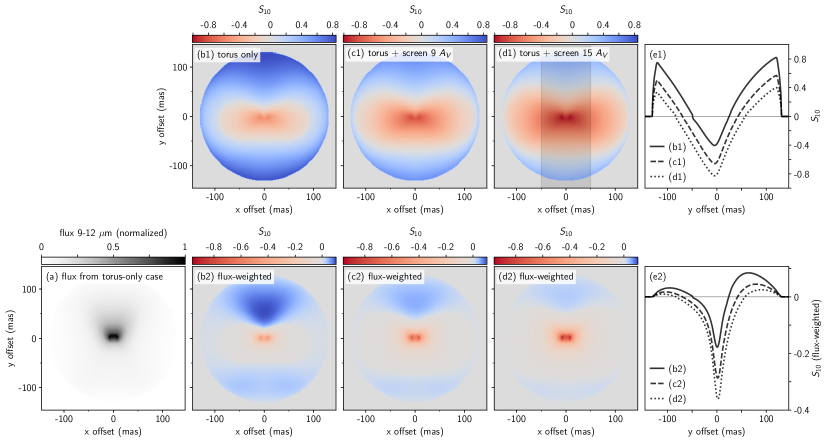
Figure 8: Spatially resolved 10 ​$\mu{\rm m}$ silicate feature strength $S_{\!10}$ obtained through simulated IFU-like observations of our NGC 1068 model, with parameters $\sigma$ = 45°, $i$ = 75°, $Y$ = 18, ${\cal N}_{0}$ = 4, $q$ = 0.08, $\tau_{\rm V}$ = 70. Full-resolution images are used, and we do not consider here degradation effects such as PSFs, noise, atmospheric conditions, etc. We assume luminosity $L_{\rm bol}=1.6\times 10^{45}~{}\rm{ergs^{-1}}$ and distance $D=14.4$ Mpc. For clarity the images are not rotated to the ${\rm PA}$ of the source, i.e., the polar direction is up. (a) Flux map of the torus model (no dust screen), integrated between 9 and 12 $\mu{\rm m}$ and normalized to its peak. (b1) Resolved $S_{\!10}$ map for the torus model. The torus near side produces silicate absorption (red colors). Polar regions generate silicate emission (blue colors). (c1) $S_{\!10}$ map for a torus model behind a (wavelength-dependent) cold screen of ISM dust with $A_{V}$ = 9 mag, similar to results from LR18. (d1) With a screen of $A_{V}$ = 15 mag. Panels (b1)–(d1) use the same color scale. The dust screen lowers silicate emission, deepens silicate absorption, and enhances the size of the area seen in absorption. (e1) Vertical mean profiles of $S_{\!10}$ over a central (vertical) band of $\pm 50$ mas width (indicated as a gray vertical stripe in panel (d1)), measured in panels b1 (solid line), c1 (dashed), and d1 (dotted). The $x$-axis corresponds to the $y$-axes in the $S_{\!10}$ maps. Positive $S_{\!10}$ values indicate silicates in emission, negative in absorption. (b2)–(d2) The panels (b1)–(d1) flux-weighted with their respective 9–12 $\mu{\rm m}$ integrated flux images (similar to the one shown in (a)). All three panels are scaled to the same color scale. (e2) Vertical $S_{\!10}$ profiles in (b2), (c2), (d2), measured in the same way as in (e1).

3 Reconstructed Interferometric Observations: Direct Image Fitting

G20 have recently published a reconstructed K-band image of NGC 1068, obtained by combining the light of four telescopes with VLTI. In contrast with previous efforts this image was reconstructed using phase closure information, i.e., it does not rely on nonphysical models of the brightness distribution.

G20 offered several models to explain the observed data. Their favored model is a simple geometric ring, where the 2.2 $\mu{\rm m}$ emission is optically thin, and emerges even from the near side of the ring. The authors derive a sublimation radius $R_{d}=0.24$ pc, inclined at $\hbox{$i$}=70\pm 5$°, and at a position angle of the disk equatorial plane ${\rm PA}=-50\pm 4$° (i.e., 50° west of north), or equivalently, ${\rm PA}=130$° E of N of the disk plane, and consequently, ${\rm PA}=40$° E of N for the disk rotation axis. The scale height was constrained by the maximum beam size to $h/r<0.14$ (which would correspond to $\sigma<8$° assuming a sharp-edge flared disk). The bolometric luminosity is rather uncertain in the literature, and the authors give a range of $0.4-4.7\times 10^{45}\,{\rm erg\,s^{-1}}$. G20 also discuss a CAT3D (Hönig & Kishimoto, 2010) model (their “Model 4”), where the observed emission predominantly arises from the far inner side of a disk/torus, and is therefore optically thick. This model is ultimately disfavored in G20 due to the harder-to-explain patchy nature of the observed emission.

We fit the GRAVITY image directly with monochromatic 2.2 $\mu{\rm m}$ Clumpy model images by varying the relevant model parameters. While fitting, we convolve the models with the effective beam (given by G20 as an $x\times y=3.1\times 1.1$ mas FWHM 2D Gaussian, rotated counter-clockwise by ${\rm PA}=48.6$° (i.e., this is the position angle of the semiminor axis of the Gaussian). We also account for correct pixelization, and take advantage of the freedom to self-similarly stretch the model image maps (“zoom factor”). In nature the “zooming” can be achieved by either changing the distance $D$ to the source – then, angular size $\theta\propto{\rm D}^{-1}$ – or by changing the AGN luminosity; in this case $\theta\propto{\rm L}^{-1/2}$, from the equation for the dust sublimation radius

$$R_{d}\ =0.4\left(\dfrac{L_{\rm bol}}{10^{45}\,{\rm erg\,s^{-1}}}\right)^{\!1/2}\left(\dfrac{T_{\rm sub}}{1500\,{\rm K}}\right)^{\!-2.6}\,{\rm(pc)}$$ (2)

(see also Paper I). With the fitted zoom factor we can directly determine the luminosity $L_{\rm bol}$ if the source distance D is fixed, and vice versa.

We perform two separate fits:

1. Model (I): fixed-origin

2. Model (II): shifting-origin

In model (I) the origin of the emission is fixed at the central pixel (0,0). In model (II) the emission pattern is allowed to shift within the image plane. This has strong implications for the resulting geometry. Performing purely morphological fitting, with both data and model images normalized to unit sum, we minimize a loss function between the data and model image (RMSE, see Appendix B) using a robust genetic algorithm (differential evolution; Storn & Price 1997).

The best-fit (convolved) model images at 2.2 $\mu{\rm m}$ are shown in Figure 9 in the second-from-left panels, for the fixed-orgin model at the top, and the shifting-origin model at the bottom. The leftmost panels show the same GRAVITY image, with the isophotes of the convolved models overplotted. The underlying unconvolved model images are shown in the third-from-left panels. Finally, the rightmost panels show the dust cloud distributions that generate the respective emission model images, scaled to their min/max ranges of clouds per LOS. All model images have of course the same pixel scale as the GRAVITY reconstructed image.

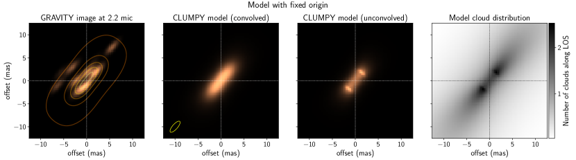
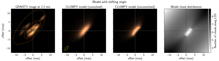
Figure 9: Fitting of the 2.2 $\mu{\rm m}$ GRAVITY image of NGC 1068 with convolved Clumpy images. The top row shows the best-fit fixed-origin model (I), and the bottom row the shifting-origin model (II). All emission images are normalized to unit sum. In all panels the dotted horizontal and vertical lines indicate the aperture origin at (0,0) offsets. The left panels show the central $25\times 25$ mas image obtained by GRAVITY. The second-from left panels show the best-fit Clumpy model images, convolved with the GRAVITY effective beam ellipse of FWHM = $3.1\times 1.1$ mas (see lower-left corner of the panel). The isophotes of these model images are shown as contours in the left panels, at 1, 10, 30, 60, 90 percent of the peak. The third-from-left panels show the underlying Clumpy model images but without convolution. Finally, the right-most panels (in gray-scale) show the underlying dust distributions, each normalized to its own range of values. All best-fit model parameters are given in Table 3.

We give all best-fit parameter values in Table 3. Because the K-band morphology does not depend on the torus radial extension $Y$, we can fix it at an arbitrary value and are setting it to $\hbox{$Y$}=18$ from SED fitting by LR18.

3.1 Results for the Fixed-origin Model (I)

For the fixed-origin model (I) all but two fitted parameters converge robustly. The results suggest a geometrically thin structure ($\hbox{$\sigma$}=24.6$° for our Gaussian soft-edge torus), viewed at $\hbox{$i$}=85.2$° inclination, and with a fitted ${\rm PA}=51.9$° of the torus axis (E of N, CCW), or ${\rm PA}=141.9$° of the torus equatorial plane. The steepness of the radial cloud number distribution is $\propto r^{-1.35}$.

Table 3: Best-fit parameters (top) and derived quantities (bottom) from direct fitting of the G20 NGC 1068 K-band image, for the fixed-origin and shifting-origin models.

Parameter	Notes	Fixed-origin	Shifting-origin
$\sigma$ (deg)		24.6	15.1a
$i$ (deg)		85.2	69.3
$Y$	(1)	fixed at 18	fixed at 18
${\cal N}_{0}$		1a	10.9b
$q$		1.35	0.47
$\tau_{\rm V}$		10a	143.5b
${\rm PA}$ (deg)	(2)	51.9 / 141.9	50.3 / 140.3
x-shift (mas)	(3)	n/a	1.37c
y-shift (mas)	(3)	n/a	-0.74d
zoom	(4)	1.037	1.344
$R_{d}$ (mas / pc)	(5)	2.26 / 0.16	2.93 / 0.20
$L_{\rm bol}\ (10^{44}\rm\,erg\,s^{-1})$		1.56	2.62

Note. — For all conversions a distance D=14.4 Mpc was adopted. Notes: (1) $Y$ is almost irrelevant for the morphology of the 2.2 $\mu{\rm m}$ image. (2) ${\rm PA}$ of torus axis / plane, E of N. (3) E-W (x) and N-S (y) shift of the AGN locus w.r.t. the origin. Modeled in (fractional) pixel space, and converted here to milliarcseconds. (4) Self-similar stretch factor applied to raw Clumpy image. (5) Angular and physical size of a dust sublimation radius. ^aUpper bound. ^bNot well-constrained. Using the mean of the last third of all minimization scheme iterations; see Appendix B for details. ^cShifted to W. ^dShifted to S.

The mean number of clouds along radial equatorial rays, ${\cal N}_{0}$, and the optical depth per cloud at visual, $\tau_{\rm V}$, do drift toward the smallest values present in our model hypercube, but do not appear to stabilize before. While we can thus not constrain them further, they do occupy the optically thin regime preferred by the G20 ring model, with the 2.2 $\mu{\rm m}$ emission emanating also from our near side of the dusty disk / torus. In fact, in our best-fit model with $\hbox{$\sigma$}=24.6$°, and taking $\hbox{${\cal N}_{0}$}=1$, there are on average only 0.96 clouds along our LOS to the central source (at $\hbox{$i$}=85.2$°), according to Equation 3 from Paper I. If their optical depth at visual (0.55 $\mu{\rm m}$) is 10, then the overall LOS optical depth in the K band is $\tau_{2.2}=0.89$ when assuming our standard silicate-graphite ISM dust, where $\tau_{2.2}/\tau_{0.55}=0.093$.

This optically thin configuration results in a K-band morphology which very closely resembles the underlying dust distribution, apparent in the two right panels in the top row of Figure 9, including the brightened edges of the central dust-free cavity. It seems challenging to reconcile such an optically thin disk with the amount of emission observed, and with the existence of co-planar and co-located maser spots (e.g., Gallimore et al., 2004) which require high densities.

The fitted zoom factor 1.037 of the images, needed in comparison to their original resolution in the model hypercube, is small. With the native Clumpy image resolution of $6\,{\rm pix}/R_{d}$ and a pixel scale of the GRAVITY image of $0.3634\,{\rm mas/pix}$, a zoom factor of 1.037 means that the dust sublimation radius $R_{d}$ subtends 2.26 mas on the sky. If we adopt the canonical distance to NGC 1068, ${\rm D}=14.4$ Mpc, then the physical size of $R_{d}$ is just 0.158 pc. This is in line with some previously derived values (e.g., Burtscher et al., 2013), but on the lower end of measurements reported in the literature. Equation (2) then yields a sublimation-setting luminosity of ${\rm L}=1.56\times 10^{44}\,{\rm erg\,s^{-1}}$. This value is even smaller than the lower limit from modeling by G20. This apparently small luminosity may have several causes, as follows.

(i) During fitting we convolve a Clumpy image with the effective beam of the telescope/instrument configuration at the time of observation, which G20 estimate as a $3.1\times 1.1$ mas FWHM elliptical beam, with the short axis inclined 48.6° E from N. This inclination is unfortunately almost identical to the ${\rm PA}$ of the 2.2 $\mu{\rm m}$ emitting dust structure; the convolution of the model image with the beam smears out the emission along its long axis, effectively increasing its apparent angular size. All the while the underlying model is smaller. In our tests this effect can increase the apparent angular size by up to 15–20 percent.

(ii) The dust sublimation temperature also enters Equation (2), and it is often assumed at 1500 K. Increasing T by just a few hundred Kelvin, e.g., through a slight over-abundance of graphites, and/or by having a slightly larger average grain size, can easily produce smaller $R_{d}$ at “standard” luminosities. For instance, ${\rm L}=0.4\times 10^{45}\,{\rm erg\,s^{-1}}$ and ${\rm T}=1800$ K (the sublimation temperature of pure graphite grains, which are likely to be the ones to survive closest to the AGN) produce $R_{d}=0.16$ pc, in line with our modeling. See, e.g., Mor et al. (2009); Heymann & Siebenmorgen (2012); Xie et al. (2015) for more discussion on the influence of dust chemistry on the dust sublimation temperature and sublimation radius in AGNs.

(iii) In our models the central illuminating source is isotropic. If it were instead emitting like an accretion disk with a $\cos\theta$ intensity fall-off with polar angle $\theta$ (see, e.g., Netzer, 1987), then the dust sublimation radius is a function of $\theta$. Kawaguchi & Mori (2010) have shown that in this case the average $R_{d}$ is only about a third of the isotropic case, and close to edge-on views it can be as small as 10 percent of the isotropic radius. The dusty disk in NGC 1068 is seen at an angle closer to edge-on, and therefore Equation (2) may not be applicable as-is, but requires an angle-dependent luminosity correction.

3.2 Results for the Shifting-origin Model (II)

For model (II) all sampled parameter ranges were kept the same, and we allowed the 2.2 $\mu{\rm m}$ emission pattern to move up to $\pm 10$ pixels in the $x$ and $y$ directions within the 69-pixel wide FOV used for fitting. A majority of the parameters have again converged robustly. ${\cal N}_{0}$ and $\tau_{\rm V}$ do not converge to a fixed value, but for later iterations of the loss function minimization their long-term mean is stable. For these two parameters we therefore adopt the mean of the final third of all iterations (over 12,000 iterations), i.e., ${\cal N}_{0}$ = 10.9 clouds and $\tau_{\rm V}$ = 143.5.

The freedom to change a bit the locus of the AGN allowed for optically thick models, where both the number of clouds along the LOS, and the optical depth of individual clouds are higher. Such models, when viewed at an angle somewhat above the equatorial plane ($i$ = 69.3° in our case), produce thermal emission morphologies that are vertically offset from the mid-plane. For our best-fit model the shifts amount to 1.37 and 0.74 milliarcseconds to the west and south, respectively.

The resulting morphology, after convolution (second-from-left panel in the lower row in Figure 9), is strikingly similar to that of model (I); the RMSE is $\sim$6 percent lower than in model (I). However, the rightmost panel in Figure 9 reveals just how different the underlying dust distribution is in this case, and by how much it had to be offset to cause this effect. In the unconvolved image (third-from-left panel) it is evident how the emission emanates just above the inner, thin-disk like part of the dust cloud distribution.

The radial cloud distribution is much flatter than in model (I), with $q$ = 0.47. This is favorable for producing emission patterns preferentially elongated in polar directions, but in this case, together with the small value of $\hbox{$\sigma$}\approx 15$°, is to first order not enough to generate the MIR elongation of 2.3:1 measured for NGC 1068 (López-Gonzaga et al., 2016); in fact, the corresponding 10 $\mu{\rm m}$ image of this model only produces $e\approx 0.4-0.5$ at the 0.1-contour level (of the peak). We discuss the issue of polar elongation in detail in Section 3 of Paper I.

The zoom factor found with this shifting-origin model (II) is 1.344, and translates to $R_{d}\ =2.93$ mas $\equiv 0.2$ pc, and $L_{\rm bol}\ =\rm 2.62\times 10^{44}\,erg\,s^{-1}$ (all for distance D = 14.4 Mpc). The same caveats (i)–(iii) for small luminosities apply as for model (I), but to a significantly lesser degree.

Overall the GRAVITY image is striking both in its unprecedented spatial resolution, but also in the fact that the circumnuclear NIR emission appears to be concentrated in only a few point-like peaks of sufficient intensity to be detected. This calls for a cautious interpretation. We emphasize that the instrumental beam smears out the observations and causes them to appear very similar for different underlying geometries. These could be either an elongated structure suggestive of a highly inclined emission ring, or a geometrically thin but optically thick flared disk where the emission arises from a narrow strip of hot cloud surface layers on the far inner side of the torus funnel. As noted in G20, extremely precise NIR astrometry of future instruments could help distinguish between the two scenarios, especially with quantitative comparison of model images such as Clumpy.

4 Summary

In this paper we computed synthetic observations of the nearby AGN NGC 1068 using images generated by the Clumpy torus models (Nenkova et al., 2008a, b). We have obtained from the respective observatories and consortia the pupil images of the JWST and Keck facilities as representatives of the best current (or nearly-current) space-based and ground-based telescopes, and of GMT, TMT, and ELT as the upcoming generation of extremely large telescopes, whose apertures will be in an unprecedented class of their own. From the pupil images we compute wavelength-dependent PSFs and discuss their general characteristics and resolving power.

We then convolve Clumpy model images with these PSFs to simulate synthetic observations of NGC 1068. We take image noise and detector pixelization into account, and employ image deconvolution techniques to obtain more realistic simulated observations. Comparison with observational results suggest that the tori in nearby AGNs, within a range of possible luminosities and distances, will be very well resolvable in the range $\sim$3–12 $\mu{\rm m}$ with the new class of extremely large telescopes, with an optimum between approximately 4 and 8 micron.

Hypercat can be used to simulate IFU-like observations. We use this capability to generate spatially and spectrally resolved images of the 10-$\mu{\rm m}$ silicate feature for a model of NGC 1068. We collapse the image cubes to maps of the feature strength as function of spatial coordinates, both without and with an intervening foreground dust screen, which seems to be suggested by observational data. Profiles of the silicate feature strength $S_{\!10}$ along the system polar direction indicate that the central 1-2 parsec generate a feature in moderate absorption, while areas above and below the torus equatorial plane produce mild silicate emission. An intervening cold dust screen deepens the absorption feature and dampens any emission features. We point out that radiative models with other emission lines (e.g., CO, H I) as computed, e.g., in Wada et al. (2016) or Williamson et al. (2020) can use this tool to compute synthetic IFU observations.

We have also fit directly the model-free K-band image of NGC 1068 obtained by GRAVITY, using convolved Clumpy images, and two different regimes (fixed-origin: optically and geometrically thin; and shifting-origin: optically thick but geometrically thin). In both cases we were able to constrain several geometrical parameters and find somewhat geometrically thin dusty structures seen closer to equatorial inclinations, at position angles of the torus axis of $\sim$50-52° E of N. Our fitting also yields scaling parameters necessary to stretch the model images self-similarly, and assuming a standard distance to NGC 1068 of 14.4 Mpc we find quite small bolometric luminosities of $1.6-2.6\times 10^{44}\,{\rm erg\,s^{-1}}$. Whether this value is robust or subject to several corrective factors, remains to be further studied.

The question of course arises whether model images fit to a single observed K-band morphology can constrain the model to such degree that it reproduces observations at other wavelengths, especially in the MIR, and whether it reproduces the broadband SED. Ideally, a fit under morphological constraints would match photometric (SED) and interferometric (morphology in certain bands) observations jointly. Our preliminary Bayesian SED fits to the data assembled in LR18 for NGC 1068, with the addition of an extinction screen, yield overall good fits, but the MIR elongations of the sampled models range only between 0.96 and 1.3. While this may be sufficient to explain elongations on scales of a few parsec, it is insufficient for the large-scale (tens of parsec) elongations observed in NGC 1068. We defer a full treatment of the joint fits to a future publication.

Building on this work we intend to expand our approach and simulate observations of a larger sample of nearby and bright AGNs with extremely large telescopes and interferometers, with the goal of constraining the torus geometry through resolved imagery.

Clumpy image hypercubes and the Hypercat software will prove useful to the AGN field and beyond. The authors welcome inquiries and help requests, as well as code and model contributions from the community.

Appendix A Synthetic Observations with Single Dish Telescopes

A.1 Generate a PSF

Hypercat provides three methods to estimate the PSF for a given telescope and wavelength.

Model-PSF (Airy function + Gaussian): The simplest PSF model of a circular telescope aperture is an Airy disk, i.e., the Fourier transform of the aperture. It is sufficient for seeing-limited observations. Focusing on 30 m class and space-based telescopes, our modeled observations will be nearly diffraction limited in the near- to mid-IR. A better PSF model is then a combination of a central Airy disk, which contains most of the power of the PSF, and a broad halo that encompasses the remaining power of the object (e.g., Hardy & Thompson, 2000). This is a semi-empirical function determined by fitting the PSF of adaptive optics observations at optical and NIR wavelengths. The free parameters of the model are the primary mirror diameter $D$, the Strehl ratio $S$, and the wavelength of the observation $\lambda$.

The full-width at half-maximum of the Airy core ${\rm FWHM_{A}}=\lambda/D$ is defined as the location of the first minimum such that

$${\rm PSF_{A}}=I^{A}_{0}J_{1}({\rm FWHM_{A}}/2)$$ (A1)

where $I^{A}_{0}$ is the peak of the core of the PSF and $J_{1}$ is the normalized first order Bessel function used by the 2D Airy function from astropy.

The normalized intensity of the peak ‘p’, for a Strehl ratio S_p, is defined as $I^{A}_{0}=e^{-\sigma_{p}^{2}}$ (see Hardy & Thompson, 2000), where $\sigma_{p}$ is the mean-square wavefront error. For typical diffraction-limited observations $\sigma_{p_{0}}=0.0745$ at a Strehl of $S_{p_{0}}=0.8$. Using these values as normalization factors of the mean-square wavefront error, $\sigma_{p_{0}}/S_{p_{0}}=0.0745/0.8=0.093125$, and we can then define the peak of the core as a function of the Strehl ratio, $S_{p}$, as $I^{A}_{0}=e^{-(0.093125/S_{p})^{2}}$. Note that the peak of PSF_A is always $<1$ because the missing flux is distributed within the halo (Gaussian profile), which is taken into account in Equation A4.

In the general 2D case the halo is given by a double Gaussian profile

$${\rm PSF_{G}}=I^{G}_{0}\exp{\left[-4\ln 2\left\{\left(\frac{x-x_{0}}{\rm FWHM_{\,G}^{\,x}}\right)^{\!2}+\left(\frac{y-y_{0}}{\rm FWHM_{\,G}^{\,y}}\right)^{\!2}\right\}\right]},$$ (A2)

which in the circular case simplifies to

$${\rm PSF_{G}}=I^{G}_{0}\exp{\left[-\frac{4\ln 2}{{\rm FWHM_{\,G}^{\,2}}}\left\{(x-x_{0})^{2}+(y-y_{0})^{2}\right\}\right]}.$$ (A3)

$I^{G}_{0}$ is the peak of the Gaussian profile

$$I^{G}_{0}=\frac{1-e^{-(0.093125/S_{p})^{2}}}{1+\left(\dfrac{D}{\rho_{0}}\right)^{\!2}}.$$ (A4)

The peak of the Gaussian profile accounts for the power missed by the central PSF, where $I_{0}^{A}+I^{G}_{0}=1$. ${\rm FWHM_{G}}$ is defined as

$${\rm FWHM_{G}}=1.22\,\frac{\lambda}{D}\left[1+\left(\frac{D}{\rho_{0}}\right)^{\!2}\right]^{1/2}.$$ (A5)

The coherent length of turbulence for short exposures is

$$\rho=\rho_{0}\left[1+0.37\left(\frac{\rho_{0}}{D}\right)^{\!1/3}\right],$$ (A6)

where $\rho_{0}$ is $\propto\lambda^{6/5}$, with typical values of $0.1-0.2$ m at 0.5 $\mu{\rm m}$. We use the normalization of 0.15 m at 0.5 $\mu{\rm m}$. The final Model-PSF is computed as $\rm PSF=PSF_{A}+PSF_{G}$ with a normalized total peak flux. Figure 10 shows an example of a PSF modeled this way for a 30 m telescope at 2.2 $\mu{\rm m}$, $\rm FWHM_{A}$ of 15 mas and Strehl ratios of 0.8 and 0.2. As expected, for larger Strehl ratios more power is accumulated in the core.

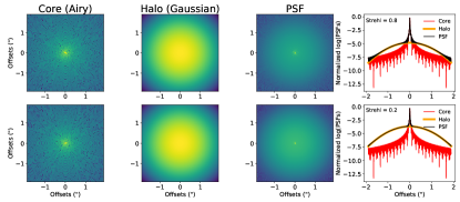
Figure 10: Model-PSF for a 30 m telescope at 2.2 $\mu{\rm m}$ with a $\rm FWHM_{A}=15$ mas and Strehl ratios of 0.8 (top) and 0.2 (bottom). From left to right the panels show the step-by-step generation of the model-PSF, using as core an Airy profile (first column), a Gaussian profile for the halo (second column), and the combined model-PSF (third column). A radial profile (forth column) for each PSF is shown. Larger Strehl ratios result in more power in the core.

Pupil-PSF (Fourier transform of the pupil): Several telescope structures such as the central obscuration of the secondary mirror, the thick spiders holding it, edges of the aperture, as well as the segmentation of the primary mirror for large telescopes, create a PSF with features far from the ideal case described above. To model the effects of these geometrical features on the PSF we can use the pupil image of the telescope. The pupil image has the shape of the primary mirror and the rest of telescope structures in front of it. The pupil images of all telescopes in Table 4 are available as FITS files in Hypercat.. Where they are available, Hypercat uses these pupil images by default. 2 shows the pupil images and the PSFs of the telescopes from Table 2. Figures 2 through 7 show in their upper rows the pupil images of several telescopes. The PSF of a real telescope can then be estimated as the Fourier transform of the pupil image

$${\rm PSF}(x^{\prime},y^{\prime})=\int{\rm Pupil}(x,y)\,e^{-j2\pi(x^{\prime}x+y^{\prime}y)}\,\hbox{${d}$}x\,\hbox{${d}$}y$$ (A7)

where $(x,y)$ and $(x^{\prime},y^{\prime})$ are the coordinates of the object and PSF plane, respectively, and the integrals are over the image domain. The PSF plane, $(x^{\prime},y^{\prime})$, is then scaled to the pixel scale in the plane of the sky at a given wavelength as $\lambda/D$, in units of arcsec. Finally, Hypercat also generates a pixelated PSF with the same pixel scale of the source.

Image-PSF (PSF image provided externally): The previous two models might lack additional components of the PSF. Some telescopes provide forward-modeled PSF images at specific wavelengths, e.g., PSFs for HST computed with the Tiny Tim tool (Krist et al., 2011), or for JWST with the WebbPSF tool (Perrin et al., 2012). Telescopes also take into account observations of point sources to characterize their PSFs at several instrument configurations. Hypercat can take such PSF images, together with a pixel scale, and apply them to the 2D Clumpy model images. A drawback of this method is that a PSF image must be provided at the exact wavelength of interest (the wavelength of the model image). Interpolation of PSF images between sampled wavelengths is not advisable as the PSF behavior can be very complex, and interpolation artifacts may be of larger magnitude than the differences between neighboring wavelengths.

This method accepts the PSF taken by a given instrumental configuration can be used to produce synthetic observations. The PSF should be provided in FITS format, where the header must have the pixel scale in units of arcsec per pixel. To compute the convolution with the model at full resolution, the PSF must also have the same FOV as the model image. Table 4 shows the available PSF modes for each telescope.

Table 4: Available PSF Modeling Modes.

Telescope	Mode
(by size)	model-PSF	pupil-PSF	image-PSF
JWST	$\circ$	$\bullet$	$\circ$
Gemini	$\circ$	-	$\circ$
Keck	$\circ$	$\bullet$	$\circ$
VLT	$\circ$	-	$\circ$
GMT	$\circ$	$\bullet$	-
TMT	$\circ$	$\bullet$	-
ELT	$\circ$	$\bullet$	$\circ$
generic	$\circ$	$\circ$	$\circ$

Note. — $\bullet$ default     $\circ$ available     - not available

A.2 PSF Convolution

Let $I_{\lambda}^{\rm mod}(x^{\prime},y^{\prime})$ be the 2D Clumpy model torus image at a given wavelength $\lambda$, at the full spatial sampling provided by Hypercat (as described in Section 2.5 of Paper I). ${\rm PSF}_{\lambda}(x^{\prime},y^{\prime})$ be the telescope PSF (Section A.1) at the same wavelength. Then the synthetically observed image is given by the convolution of the full resolution model and the PSF

$$I_{\lambda}^{\rm obs}(x,y)=I_{\lambda}^{\rm mod}(x^{\prime},y^{\prime})\ast{\rm PSF}_{\lambda}(x^{\prime},y^{\prime})=\int I_{\lambda}^{\rm mod}(x^{\prime},y^{\prime})\,{\rm PSF}_{\lambda}(x-x^{\prime},y-y^{\prime})\,\hbox{${d}$}x^{\prime}\,\hbox{${d}$}y^{\prime}$$ (A8)

where the PSF has been normalized to unity

$$\int\limits_{-\infty}^{\infty}\int\limits_{-\infty}^{\infty}{\rm PSF_{\lambda}}(x,y)\,\hbox{${d}$}x\,\hbox{${d}$}y=1$$ (A9)

and has the same spatial sampling as the 2D Clumpy torus image, $I_{\lambda}^{\rm mod}(x^{\prime},y^{\prime})$. The User Manual shows in detail how the pupil images and PSFs can be incorporated into a workflow.

A.3 Detector Pixelization

While the PSF-convolved image is at the same (high) angular resolution as the model image, the detector can only generate discrete elements of resolution given by its pixel scale. We produce a pixelated image given the instrumental configuration shown in Table 2. Specifically, we down-sample the PSF-convolved image to the desired detector pixel scale using a spline interpolation of order 3. The PSF-convolved image with a $N_{x}\times N_{y}=241\,{\rm pix}\times 241\,{\rm pix}$ and pixel scale $\Delta{\rm px_{full}}$ is then pixelated to achieve the detector pixel scale $\Delta{\rm px_{det}}$, by using the pixel conversion $\Delta{\rm px_{obs}}=\Delta{\rm px_{\rm det}}/\Delta{\rm px_{full}}$. The final pixelated image has $N^{\prime}_{x}\times N^{\prime}_{y}=N_{x}/\Delta{\rm px_{obs}}\times N_{y}/\Delta{\rm px_{obs}}$ pixels². Figure 4 (middle row) shows an example of this procedure using the 2D PSF-convolved Clumpy model image of NGC 1068 obtained in Appendix A.2, and pixelated to the Nyquist sampling of TMT at 3.45 $\mu{\rm m}$.

A.4 Noise

In a real measurement noise must be considered due to, for instance, detector fluctuations, atmospheric emission and transmission, etc. In Hypercat we approximate the (optional) noise contribution as background-limited. The added noise pattern is a Gaussian with mean $\mu=0$ and standard deviation $\sigma=f\times\rm max(image)/SNR$, that is, the noise level is specified by the desired SNR, for a signal given as fraction $f$ of the peak pixel value. The default fraction is $f=1$, i.e., the actual peak pixel value, but it can be set within $\left]0,1\right]$. This is useful for instance if the observer is interested in the SNR in the extended emission of the source, rather than at its peak. Figure 4 panel G shows an example of this procedure using the convolved and pixelated synthetic observations of NGC 1068 with TMT at 3.45 $\mu{\rm m}$ (see Section A.3), with a SNR of 20 at the peak pixel (and noise level fraction $f=1$).

A.5 Deconvolution

Deconvolution techniques make it possible to remove the PSF contribution from (semi-)resolved observations to obtain finer details of the astrophysical object. The Richardson-Lucy algorithm (Richardson, 1972; Lucy, 1974) is one of the most commonly used methods for image deconvolution in astronomy. We use it on the synthetic observations generated by Hypercat, both for the pixelated (Section A.3) and the noisy (Section A.4) images. The user can introduce the number of iterations required to produce a final deconvolved image based on their own criteria. Figures 6 and 7 show examples of this procedure using the pixelated synthetic and noisy observations of NGC 1068 with 10 iterations. For larger iterations the algorithm produces artifacts at the lower surface brightness, while for small iterations the algorithm did not have time to converge. Our criterion was to stop the iterations once the final image did recover the overall shape of the contour at the level of 0.01 $\times$ the peak flux of the full resolution image shown in Figure 6.

Appendix B Direct Image Fitting

The direct image fitting described in Section 3 minimizes a loss function, in our case the Root Mean Square Error

$$RMSE=\sqrt{\langle(D-M)^{2}\rangle}\,,$$ (B1)

where $\langle\cdot\rangle$ indicates the mean over the squared residuals between data $D$ and model $M$ (pixel values of each). We minimize Equation (B1) using differential evolution, implemented in scipy.optimize.differential_evolution. This genetic algorithm (Storn & Price, 1997) proves very robust, is reasonably fast even in high dimensions, and is easily parallelizable. Figure 11 shows the convergence behavior over the iteration number for our shifting-origin model (II).

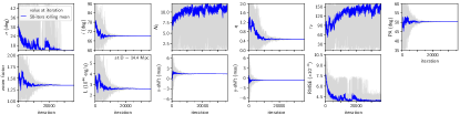
Figure 11: Fitting of the 2.2 $\mu{\rm m}$ GRAVITY image with convolved Clumpy images, for the case of the shifting-origin model (II); see Section 3 for details. The panels show the convergence behavior of the differential evolution minimization, with a Root Mean Square Error (RMSE, last panel) loss function. The $Y$ parameter was fixed at $\hbox{$Y$}\ =18$. $L$ is computed from the zoom factor after the fitting, and assuming a distance D = 14.4 Mpc to NGC 1068.

References

- Alonso-Herrero et al. (2011) Alonso-Herrero, A., Ramos Almeida, C., Mason, R., et al. 2011, ApJ, 736, 82, doi: 10.1088/0004-637X/736/2/82
- Alonso-Herrero et al. (2016) Alonso-Herrero, A., Esquej, P., Roche, P. F., et al. 2016, MNRAS, 455, 563, doi: 10.1093/mnras/stv2342
- Angel et al. (2003) Angel, J. R. P., Burge, J. H., Codona, J. L., Davison, W. B., & Martin, B. 2003, in Proc. SPIE, Vol. 4840, Future Giant Telescopes, ed. J. R. P. Angel & R. Gilmozzi, 183–193, doi: 10.1117/12.459862
- Antonucci (1993) Antonucci, R. 1993, ARA&A, 31, 473, doi: 10.1146/annurev.aa.31.090193.002353
- Asmus et al. (2015) Asmus, D., Gandhi, P., Hönig, S. F., Smette, A., & Duschl, W. J. 2015, MNRAS, 454, 766, doi: 10.1093/mnras/stv1950
- Astropy Collaboration et al. (2013) Astropy Collaboration, Robitaille, T. P., Tollerud, E. J., et al. 2013, A&A, 558, A33, doi: 10.1051/0004-6361/201322068
- Bland-Hawthorn et al. (1997) Bland-Hawthorn, J., Freeman, K. C., & Quinn, P. J. 1997, ApJ, 490, 143, doi: 10.1086/304865
- Burtscher et al. (2013) Burtscher, L., Meisenheimer, K., Tristram, K. R. W., et al. 2013, A&A, 558, A149, doi: 10.1051/0004-6361/201321890
- Collette et al. (2019) Collette, A., et al. 2019, h5py: HDF5 for Python. http://www.h5py.org/
- Fritz et al. (2006) Fritz, J., Franceschini, A., & Hatziminaoglou, E. 2006, MNRAS, 366, 767, doi: 10.1111/j.1365-2966.2006.09866.x
- Gallimore et al. (2004) Gallimore, J. F., Baum, S. A., & O’Dea, C. P. 2004, ApJ, 613, 794, doi: 10.1086/423167
- García-Burillo et al. (2016) García-Burillo, S., Combes, F., Ramos Almeida, C., et al. 2016, ApJ, 823, L12, doi: 10.3847/2041-8205/823/1/L12
- González-Martín et al. (2013) González-Martín, O., Rodríguez-Espinosa, J. M., Díaz-Santos, T., et al. 2013, A&A, 553, A35, doi: 10.1051/0004-6361/201220382
- Goulding et al. (2012) Goulding, A. D., Alexander, D. M., Bauer, F. E., et al. 2012, ApJ, 755, 5, doi: 10.1088/0004-637X/755/1/5
- Gratadour et al. (2015) Gratadour, D., Rouan, D., Grosset, L., Boccaletti, A., & Clénet, Y. 2015, A&A, 581, L8, doi: 10.1051/0004-6361/201526554
- Gravity Collaboration et al. (2020) Gravity Collaboration, Pfuhl, O., Davies, R., et al. 2020, A&A, 634, A1, doi: 10.1051/0004-6361/201936255
- Hao et al. (2007) Hao, L., Weedman, D. W., Spoon, H. W. W., et al. 2007, ApJ, 655, L77, doi: 10.1086/511973
- Hao et al. (2005) Hao, L., Spoon, H. W. W., Sloan, G. C., et al. 2005, ApJ, 625, L75, doi: 10.1086/431227
- Hardy & Thompson (2000) Hardy, J. W., & Thompson, L. 2000, Physics Today, 53, 69, doi: 10.1063/1.883053
- Harris et al. (2020) Harris, C. R., Millman, K. J., van der Walt, S. J., et al. 2020, Nature, 585, 357, doi: 10.1038/s41586-020-2649-2
- Heymann & Siebenmorgen (2012) Heymann, F., & Siebenmorgen, R. 2012, ApJ, 751, 27, doi: 10.1088/0004-637X/751/1/27
- Hönig et al. (2006) Hönig, S. F., Beckert, T., Ohnaka, K., & Weigelt, G. 2006, A&A, 452, 459, doi: 10.1051/0004-6361:20054622
- Hönig & Kishimoto (2010) Hönig, S. F., & Kishimoto, M. 2010, A&A, 523, A27, doi: 10.1051/0004-6361/200912676
- Hönig & Kishimoto (2017) —. 2017, ApJ, 838, L20, doi: 10.3847/2041-8213/aa6838
- Hönig et al. (2012) Hönig, S. F., Kishimoto, M., Antonucci, R., et al. 2012, ApJ, 755, 149, doi: 10.1088/0004-637X/755/2/149
- Hönig et al. (2010) Hönig, S. F., Kishimoto, M., Gandhi, P., et al. 2010, A&A, 515, A23, doi: 10.1051/0004-6361/200913742
- Hönig et al. (2013) Hönig, S. F., Kishimoto, M., Tristram, K. R. W., et al. 2013, ApJ, 771, 87, doi: 10.1088/0004-637X/771/2/87
- Hunter (2007) Hunter, J. D. 2007, Computing In Science & Engineering, 9, 90, doi: 10.1109/MCSE.2007.55
- Ichikawa et al. (2015) Ichikawa, K., Packham, C., Ramos Almeida, C., et al. 2015, ApJ, 803, 57, doi: 10.1088/0004-637X/803/2/57
- Imanishi et al. (2018) Imanishi, M., Nakanishi, K., Izumi, T., & Wada, K. 2018, ApJ, 853, L25, doi: 10.3847/2041-8213/aaa8df
- Jaffe et al. (2004) Jaffe, W., Meisenheimer, K., Röttgering, H. J. A., et al. 2004, Nature, 429, 47, doi: 10.1038/nature02531
- Kawaguchi & Mori (2010) Kawaguchi, T., & Mori, M. 2010, ApJ, 724, L183, doi: 10.1088/2041-8205/724/2/L183
- Krist et al. (2011) Krist, J. E., Hook, R. N., & Stoehr, F. 2011, in Proc. SPIE, Vol. 8127, Optical Modeling and Performance Predictions V, 81270J, doi: 10.1117/12.892762
- Krolik & Begelman (1988) Krolik, J. H., & Begelman, M. C. 1988, ApJ, 329, 702, doi: 10.1086/166414
- Krügel (2009) Krügel, E. 2009, A&A, 493, 385, doi: 10.1051/0004-6361:200809976
- Leftley et al. (2018) Leftley, J. H., Tristram, K. R. W., Hönig, S. F., et al. 2018, ApJ, 862, 17, doi: 10.3847/1538-4357/aac8e5
- Levenson et al. (2007) Levenson, N. A., Sirocky, M. M., Hao, L., et al. 2007, ApJ, 654, L45, doi: 10.1086/510778
- Lira et al. (2013) Lira, P., Videla, L., Wu, Y., et al. 2013, ApJ, 764, 159, doi: 10.1088/0004-637X/764/2/159
- López-Gonzaga et al. (2016) López-Gonzaga, N., Burtscher, L., Tristram, K. R. W., Meisenheimer, K., & Schartmann, M. 2016, A&A, 591, A47, doi: 10.1051/0004-6361/201527590
- López-Gonzaga et al. (2014) López-Gonzaga, N., Jaffe, W., Burtscher, L., Tristram, K. R. W., & Meisenheimer, K. 2014, A&A, 565, A71, doi: 10.1051/0004-6361/201323002
- Lopez-Rodriguez et al. (2015) Lopez-Rodriguez, E., Packham, C., Jones, T. J., et al. 2015, MNRAS, 452, 1902, doi: 10.1093/mnras/stv1410
- Lopez-Rodriguez et al. (2016) Lopez-Rodriguez, E., Packham, C., Roche, P. F., et al. 2016, MNRAS, 458, 3851, doi: 10.1093/mnras/stw541
- Lopez-Rodriguez et al. (2018) Lopez-Rodriguez, E., Fuller, L., Alonso-Herrero, A., et al. 2018, ApJ, 859, 99, doi: 10.3847/1538-4357/aabd7b
- Lopez-Rodriguez et al. (2020) Lopez-Rodriguez, E., Alonso-Herrero, A., García-Burillo, S., et al. 2020, ApJ, 893, 33, doi: 10.3847/1538-4357/ab8013
- Lucy (1974) Lucy, L. B. 1974, AJ, 79, 745, doi: 10.1086/111605
- Mason et al. (2006) Mason, R. E., Geballe, T. R., Packham, C., et al. 2006, ApJ, 640, 612, doi: 10.1086/500299
- Mason et al. (2009) Mason, R. E., Levenson, N. A., Shi, Y., et al. 2009, ApJ, 693, L136, doi: 10.1088/0004-637X/693/2/L136
- Mor et al. (2009) Mor, R., Netzer, H., & Elitzur, M. 2009, ApJ, 705, 298, doi: 10.1088/0004-637X/705/1/298
- Nenkova et al. (2002) Nenkova, M., Ivezić, Ž., & Elitzur, M. 2002, ApJ, 570, L9, doi: 10.1086/340857
- Nenkova et al. (2008a) Nenkova, M., Sirocky, M. M., Ivezić, Ž., & Elitzur, M. 2008a, ApJ, 685, 147, doi: 10.1086/590482
- Nenkova et al. (2008b) Nenkova, M., Sirocky, M. M., Nikutta, R., Ivezić, Ž., & Elitzur, M. 2008b, ApJ, 685, 160, doi: 10.1086/590483
- Netzer (1987) Netzer, H. 1987, MNRAS, 225, 55, doi: 10.1093/mnras/225.1.55
- Nikutta et al. (2009) Nikutta, R., Elitzur, M., & Lacy, M. 2009, ApJ, 707, 1550, doi: 10.1088/0004-637X/707/2/1550
- Nikutta et al. (2021) Nikutta, R., Lopez-Rodriguez, R., Ichikawa, K., et al. 2021, ApJ (Paper I)
- Packham et al. (1997) Packham, C., Young, S., Hough, J. H., Axon, D. J., & Bailey, J. A. 1997, MNRAS, 288, 375, doi: 10.1093/mnras/288.2.375
- Perrin et al. (2012) Perrin, M. D., Soummer, R., Elliott, E. M., Lallo, M. D., & Sivaramakrishnan, A. 2012, in Proc. SPIE, Vol. 8442, Space Telescopes and Instrumentation 2012: Optical, Infrared, and Millimeter Wave, 84423D, doi: 10.1117/12.925230
- Price-Whelan et al. (2018) Price-Whelan, A. M., Sipőcz, B. M., Günther, H. M., et al. 2018, AJ, 156, 123, doi: 10.3847/1538-3881/aabc4f
- Prieto et al. (2014) Prieto, M. A., Mezcua, M., Fernández-Ontiveros, J. A., & Schartmann, M. 2014, MNRAS, 442, 2145, doi: 10.1093/mnras/stu1006
- Raban et al. (2009) Raban, D., Jaffe, W., Röttgering, H., Meisenheimer, K., & Tristram, K. R. W. 2009, MNRAS, 394, 1325, doi: 10.1111/j.1365-2966.2009.14439.x
- Ramos Almeida et al. (2011) Ramos Almeida, C., Levenson, N. A., Alonso-Herrero, A., et al. 2011, ApJ, 731, 92, doi: 10.1088/0004-637X/731/2/92
- Richardson (1972) Richardson, W. H. 1972, Journal of the Optical Society of America (1917-1983), 62, 55
- Roche et al. (2006) Roche, P. F., Packham, C., Telesco, C. M., et al. 2006, MNRAS, 367, 1689, doi: 10.1111/j.1365-2966.2006.10072.x
- Schartmann et al. (2008) Schartmann, M., Meisenheimer, K., Camenzind, M., et al. 2008, A&A, 482, 67, doi: 10.1051/0004-6361:20078907
- Siebenmorgen et al. (2005) Siebenmorgen, R., Haas, M., Krügel, E., & Schulz, B. 2005, A&A, 436, L5, doi: 10.1051/0004-6361:200500109
- Siebenmorgen et al. (2015) Siebenmorgen, R., Heymann, F., & Efstathiou, A. 2015, A&A, 583, A120, doi: 10.1051/0004-6361/201526034
- Simpson et al. (2002) Simpson, J. P., Colgan, S. W. J., Erickson, E. F., et al. 2002, ApJ, 574, 95, doi: 10.1086/340946
- Spoon et al. (2007) Spoon, H. W. W., Marshall, J. A., Houck, J. R., et al. 2007, ApJ, 654, L49, doi: 10.1086/511268
- Stalevski et al. (2016) Stalevski, M., Ricci, C., Ueda, Y., et al. 2016, MNRAS, 458, 2288, doi: 10.1093/mnras/stw444
- Storn & Price (1997) Storn, R., & Price, K. 1997, Journal of Global Optimization, 11, 341 , doi: https://doi.org/10.1023/A:1008202821328
- Sturm et al. (2005) Sturm, E., Schweitzer, M., Lutz, D., et al. 2005, ApJ, 629, L21, doi: 10.1086/444359
- Teplitz et al. (2006) Teplitz, H. I., Armus, L., Soifer, B. T., et al. 2006, ApJ, 638, L1, doi: 10.1086/500791
- Tristram et al. (2014) Tristram, K. R. W., Burtscher, L., Jaffe, W., et al. 2014, A&A, 563, A82, doi: 10.1051/0004-6361/201322698
- Urry & Padovani (1995) Urry, C. M., & Padovani, P. 1995, PASP, 107, 803, doi: 10.1086/133630
- Vinković et al. (2003) Vinković, D., Ivezić, Ž., Miroshnichenko, A. S., & Elitzur, M. 2003, MNRAS, 346, 1151, doi: 10.1111/j.1365-2966.2003.07159.x
- Virtanen et al. (2020) Virtanen, P., Gommers, R., Oliphant, T. E., et al. 2020, Nature Methods, 17, 261, doi: 10.1038/s41592-019-0686-2
- Wada et al. (2016) Wada, K., Schartmann, M., & Meijerink, R. 2016, ApJ, 828, L19, doi: 10.3847/2041-8205/828/2/L19
- Williamson et al. (2020) Williamson, D., Hönig, S., & Venanzi, M. 2020, ApJ, 897, 26, doi: 10.3847/1538-4357/ab989e
- Wu et al. (2009) Wu, Y., Charmandaris, V., Huang, J., Spinoglio, L., & Tommasin, S. 2009, ApJ, 701, 658, doi: 10.1088/0004-637X/701/1/658
- Xie et al. (2015) Xie, Y., Li, A., Hao, L., & Nikutta, R. 2015, ApJ, 808, 145, doi: 10.1088/0004-637X/808/2/145