Spectroscopic Signatures of Strong Correlations and Unconventional Superconductivity in Twisted Trilayer Graphene

Magic-angle twisted trilayer graphene (MATTG) has emerged as a novel moiré material that exhibits both strong electronic correlations and unconventional superconductivity^{1, 2}. However, spectroscopic studies of its electronic properties are lacking, and the nature of superconductivity and the corresponding order parameter in this system remain elusive. Here we perform high-resolution scanning tunneling microscopy and spectroscopy of MATTG and reveal extensive regions of atomic reconstruction that favor mirror-symmetric stacking. In these regions we observe a cascade of symmetry-breaking electronic transitions and doping-dependent band structure deformations similar to those realized in magic-angle bilayers, as expected theoretically given the commonality of flat bands^{3, 4}. More strikingly, in a density window spanning two to three holes per moiré unit cell, spectroscopic signatures of superconductivity are manifest as pronounced dips in the tunneling conductance at the Fermi level accompanied by coherence peaks that become gradually suppressed at elevated temperatures and magnetic fields. The observed evolution of the conductance with doping is consistent with a gate-tunable transition from a gapped to a nodal superconductor, which we show theoretically is compatible with a sharp transition from a Bardeen-Cooper-Schrieffer (BCS) to a Bose-Einstein-condensation (BEC) superconductor with a nodal order parameter. Within this doping window we also detect peak-dip-hump structures suggesting that superconductivity is driven by strong coupling to bosonic modes of MATTG. Our results pave the way for further understanding of superconductivity and correlated states in graphene-based moiré structures beyond twisted bilayers, where unconventional superconductivity and nodal pairing are also reported⁵.

Figure 1a,b,c shows a schematic of the scanning tunneling microscopy (STM) setup and MATTG topography formed by alternatingly rotating three graphene layers by $\theta=1.5\degree$^{3, 1, 2}, resulting in a moiré wavelength of $L_{m}=a/[2\sin(\theta/2)]\approx 9$ nm, where $a=0.246$ nm is the graphene crystal lattice (see Methods, sections 1 and 2 for fabrication and measurement details). Since MATTG is composed of three layers, two independent moiré patterns can in principle arise and, moreover, possible offsets between the first and third layers, could result in even more complex outcomes. Surprisingly, however, we consistently observe a unique triangular moiré lattice, with no sign of an additional underlying moiré pattern, signaling the formation of a single predominantly A-tw-A configuration in which the first and third layers are aligned and second layer is twisted by $\theta$ (Fig. 1c,d). This observation suggests that mirror symmetric A-tw-A stacking is preferred, in line with previous ab-initio theory calculations⁶ and transport measurements^{1, 2}. Additionally, in large-scale topographies, we occasionally observe stripe-like features (Fig. 1b) that are not reported in twisted bilayers. We attribute these stripes to domain boundaries where strain in the top and bottom layers arises as a result of the the atomic reconstruction necessary to maintain A-tw-A stacking across the domains (Fig. 1e; Methods, section 3).

Spectroscopy of MATTG (Fig. 1f) upon electrostatic doping (controlled by the gate voltage $V_{\rm Gate}$) is similar to magic-angle twisted bilayer graphene (MATBG) in many respects—a reflection of the alternating-angle stacking of the trilayer, which conspires to form spin/valley-degenerate flat bands, together with additional dispersive Dirac cones^{3, 6}. The two Van Hove singularities (VHSs) originating from those flat bands, detected as peaks in tunneling conductance $dI/dV$, are pushed apart at the charge neutrality point (CNP, $\nu=0$) compared to full filling of four electrons (holes) per moiré unit cell ($\nu=\pm 4$). The approximately fivefold change in VHS separation indicates that the partially filled flat band structure is largely determined by electronic correlations in analogy with the behaviour seen in MATBG^{7, 8, 9, 10}. A well-developed cascade of flavor symmetry-breaking phase transitions^{11, 12} is also observed (Fig. 1f). The overall spectroscopic similarities between MATTG and MATBG suggest that the flat bands in MATTG dominate the local density of states (LDOS) in this regime. We do nevertheless detect subtle signatures of the expected additional Dirac cones. Most obviously, contrary to twisted bilayers, at $\nu=\pm 4$ the LDOS is neither completely suppressed nor accompanied by quantum dot formation¹³ (see Extended Data Fig. 1)—indicating the presence of gapless states intervening between the flat bands and remote dispersive bands.

The LDOS at the Fermi level measured at finite magnetic fields¹³ provides further signatures of the additional Dirac cones in MATTG (Fig. 2a). We resolve clear Landau fans emanating from zero field around $\nu=0,\pm 4$ along with $\nu=+1,\pm 2$; the latter signal Fermi surface reconstructions due to flavour symmetry-breaking transitions in agreement with conclusions of transport studies^{1, 2}. The main fan sequence originating from $\nu=+4$ is $+2,+6,\dots$ ($-2,-6,\dots$ for $\nu=-4$) instead of the $0,+4,\dots$ pattern typically seen in MATBG devices. The relative Chern-number shift of $2$ naturally arises from the zeroth Landau level (LL) associated with the additional Dirac cones, which contribute to the total Chern number at $\nu=\pm 4$. Finite-bias spectroscopy in magnetic fields more directly exposes the presence of additional Dirac cones in the spectrum (Fig. 2c,d). Here we can clearly identify the $N=0,\pm 1,\pm 2,\dots$ Landau levels originating from the Dirac dispersion; the increase of Landau level separation with field (Fig. 2f) confirms the linear dispersion and yields a monolayer-graphene Dirac velocity in agreement with theoretical expectations^{4, 6}.

Spectroscopy at finite magnetic fields additionally uncovers filling-dependent band structure renormalization in MATTG^{14, 15}. The effect originates from the inhomogeneous real-space charge distribution associated with different energy eigenstates: the majority of the weight of the flat-band states (including those near the VHS) are spatially located on the AAA moiré sites, whereas the additional Dirac cones and flat-band states in the immediate vicinity of the $\gamma$ point are more uniformly distributed (see Extended Data Fig. 2). Electrostatic doping thereby gives rise to a Hartree potential that modifies the band structure in a manner that promotes charge uniformity throughout the unit cell. In twisted bilayer graphene it was found¹⁶ that this potential generates additional band deformations ^{17, 18, 19, 20}. Our simulations capture a similar band-renormalization in MATTG accompanied by a displacement of the additional Dirac cones away from the flat bands^{14, 15} (Fig. 2b). Both effects—band deformations (Fig. 2e-h) and the relative Dirac cone shift—are clearly confirmed in our measurements. Importantly, the position of the Dirac point obtained from tracking the zeroth Landau level (Fig. 2c,d) falls within $\pm 50$ meV depending on the exact doping; it resides below the lower flat-band VHS at $\nu=+4$ but moves above the upper flat-band VHS at $\nu=-4$. This pronounced shift may explain the large bandwidth estimate of $>100$ meV from Ref. 1 (see Methods, section 4B,C for additional discussion). Finally, we note that the Landau levels from the Dirac cones appear unaltered by the cascade of phase transitions in the flat bands, suggesting that the flat-band and Dirac sectors are not strongly coupled by interactions²¹.

Having established the foundational properties of MATTG band structure, we now turn to the doping range $-3\lesssim\nu\lesssim-2$, where significant suppression of the tunneling conductance is observed (Fig. 3a). We identify two main doping regions—one at $-2.1<\nu<-1.9$ and the other at $-3<\nu<-2.2$. The former interval, around $\nu\approx-2$, exhibits a correlation-induced gap accompanied by Coulomb diamonds and nearly horizontal resonance peaks, signaling the formation of quantum dots and a correlated insulating state^{22, 13}, despite the presence of the additional Dirac cones.

Throughout the second interval, $-3<\nu<-2.2$, the tunneling conductance minimum is well-pinned to the Fermi energy ($V_{\rm Bias}=0$) despite the large change in filling. Strikingly, this suppression is accompanied by peak structures symmetrically placed around the Fermi energy as line traces show in Fig. 3b,c (note that the spectra taken at $-2.1<\nu<-1.9$ do not exhibit these symmetric peaks; see Extended Data Fig. 4). The presence of such sharp narrow peaks—which strongly resemble coherence peaks in superconductors and occur in the filling range where transport experiments observe superconductivity^{1, 2}—leads us to attribute this spectroscopic signature to superconductivity in MATTG.

Temperature and magnetic field dependence of the tunneling spectra (Fig. 3d-g) corroborates the connection to superconductivity while also establishing its unconventional nature. As the temperature is increased, the coherence peaks on both sides of the Fermi energy subside gradually until $2-2.5$ K (close to the maximum critical temperature reported in transport¹), where the hole-side peak completely disappears (Fig. 3d,f) and the zero-bias conductance exhibits a visible upturn (Fig. 3e; see also Extended Data Fig. 5 for more data). Suppressed zero-bias conductance together with a significantly broadened electron-side peak nevertheless survives at this temperature; both features are washed out only around $T^{*}\approx 7$ K (Fig. 3e,f). Persistent conductance suppression beyond the disappearance of coherence peaks is typically interpreted as evidence of a pseudogap phase characteristic of unconventional superconductors such as cuprates or thin films of disordered alloys^{23, 24} (see Extended Data Fig. 6 for data near $\nu=+2$). Our observation of two different temperature scales is consistent with the existence of superconducting and pseudogap phases in MATTG. In any case, the gradual disappearance of the coherence peak with temperature reaffirms its superconducting origin.

Denoting the coherence peak-to-coherence peak distance as $2\Delta$, we find maximal $\Delta\approx 1.6~{}\text{meV}$ near $\nu=-2.4$ (Fig. 3h). The overall doping dependence of the spectroscopic gap resembles the doping dependence of the critical temperature $T_{C}$^{1, 2}, which also peaks around $\nu\approx-2.4$, suggesting a correlation between these two quantities. The maximal critical temperature $T_{C}\approx 2-2.5$ K from transport¹ yields a ratio $2\Delta/k_{B}T_{C}\approx 15-19$ ($k_{B}$ is Boltzmann’s constant) that far exceeds the conventional BCS value ($\approx 3.5$)—highlighting the strong-coupling nature of superconductivity in MATTG. The measured spectroscopic gaps also imply a maximum Pauli limit of $\sim 10~{}\text{T}$ for the destruction of spin-singlet superconductivity.

The coherence peak height at base temperature ($T=400$ mK) also gradually decreases with perpendicular magnetic field, similar to tunneling conductance measurements through MATBG junctions²⁵. We observe that the coherence peaks are greatly diminished by $1$ T and therefore infer a critical field $B_{C}\gtrsim 1~{}\text{T}$ at $\nu\approx-2.4$ (Fig. 3g; see also Extended Data Fig. 5). This result is compatible with the small Ginzburg-Landau coherence length of $\xi_{\rm GL}\approx 12~{}\text{nm}$ reported around optimal doping¹ upon using the naive estimate $B_{C}\approx\Phi_{0}/{2\pi\xi_{\rm GL}^{2}}\sim 2~{}\text{T}$, where $\Phi_{0}$ is the magnetic flux quantum. Note that LDOS suppression without coherence peaks persists up to much larger fields (Extended Data Fig. 5f,g).

Interestingly, suppressed tunneling conductance within the coherence peaks typically evolves from a U-shaped profile at $-2.4\lesssim\nu<-2.2$ (Fig. 3b) to a V-shaped profile at $-3\lesssim\nu\lesssim-2.4$ (Fig. 3c), suggesting two distinct superconducting regimes. Magnetic-field dependence of the tunneling conductance further distinguishes these regimes: the field more efficiently suppresses the spectroscopic gap in the V-shaped window compared to the U-shaped window (Extended Data Fig. 5). The V-shaped tunneling spectra resemble that of cuprates and can be well-fit using the standard Dynes formula²⁶ with a pairing order parameter that yields gapless nodal excitations as reported in twisted bilayer graphene⁵ (Fig. 3c and Extended Data Fig. 7; see Methods, section 5). The enhanced conductance suppression of the U-shaped spectra instead suggests the onset of a fully gapped superconducting state. One logical possibility is that the U- and V-shaped regimes admit distinct superconducting order parameter symmetries that underlie a transition from a gapped to gapless paired state on hole doping (similar behavior has been proposed for cuprates ²⁷). We stress, however, that a standard isotropic s-wave pairing order parameter fails to adequately fit the U-shaped spectra, though reasonable agreement can be obtained by postulating a mixture of $s$-wave and nodal order parameters or a $d+id$-like order parameter (see Methods, section 5 and Extended Data Fig. 7).

We point here to an alternative explanation whereby the U- to V-shaped regimes can be understood in the context of BEC and BCS phases with a single nodal order parameter. In this scenario, starting from the correlation-induced gapped flat bands at $\nu=-2$, hole doping initially introduces strongly bound Cooper pair ‘molecules,’ rather than simply depleting the lower flat band; i.e., the chemical potential remains within the gap of the correlated insulator (Fig. 3i). Condensing the Cooper pair molecules yields a BEC-like superconducting state that we assume exhibits a nodal order parameter. Crucially, the original correlation-induced flat-band gap nevertheless precludes gapless quasiparticle excitations. Further hole doping eventually begins depleting the lower flat band (Fig. 3j), at which point the system transitions to a BCS-like superconductor. Here, Cooper pair formation onsets at the Fermi energy, and the nodal order parameter allows for gapless quasiparticle excitations. (When compared against a BEC phase, we use ‘BCS’ to describe a superconductor for which the chemical potential intersects a band, independent of the pairing mechanism or coupling strength.) The gapped versus gapless distinction implies that the U- and V-shaped regimes are separated by a clear transition^{28, 29} as opposed to the well-studied BEC-BCS crossover^{30, 31} operative when both regimes are fully gapped and not topologically distinct.

We phenomenologically model such a transition by considering the tunneling conductance of a system with electron and hole bands that experience doping-dependent band separation and nodal pairing chosen to mimic experiment; for details see Methods, section 6.2. In the fully gapped BEC phase, this model yields U-shaped tunneling spectra (Fig. 3k) that qualitatively match the measured conductance. Indeed, as in experiment, the conductance gap profile does not fit an isotropic $s$-wave pairing amplitude well due to the additional structure from the nodal order parameter. When the system enters the BCS phase (the chemical potential lies inside the band), the gapless nodal BCS phase instead yields a V-shaped tunneling profile (Fig. 3l) that also qualitatively matches the experiment. This interpretation of the U- to V-shaped transition is bolstered by transport measurements¹ that reveal two regimes for the Ginzburg-Landau coherence length (see Methods, section 6.2).

Adjacent to the coherence peaks, we observe dip-hump features in the tunneling conductance that persist over a broad doping range (Fig. 4). The positive and negative voltage dips are typically symmetric in energy, independent of filling—ruling out the possibility that the dip-hump structure is intrinsic to background density of states. Similar dip-hump features are observed spectroscopically in a range of both conventional strongly coupled phonon superconductors^{32, 33} as well as unconventional cuprate, iron-based and heavy fermion superconductors^{34, 35, 36, 37, 38, 39}. Such features are usually interpreted as a signature of bosonic modes that mediate superconductivity and can thus provide key insight into the pairing mechanism^{40, 41}. If a superconductor exhibits strong electron-boson coupling, dip-hump signatures are expected to appear at energies $\Pi=\Delta+\Omega$, where $\Delta$ is the spectroscopic gap defined above and $\Omega$ is the bosonic-mode excitation energy^{42, 40, 41}. We extract the energy of the mode $\Omega=\Pi-\Delta$ as a function of doping (Fig. 4b) and find it to be correlated with $\Delta$. In the V-shaped region, $\Omega/(2\Delta)$ anticorrelates with the spectroscopic gap—in agreement with the trends seen in cuprates and iron-based compounds^{34, 35, 38, 37, 43}—and is bounded to be less than $1$ (Fig. 4c). The upper bound of $\Omega/(2\Delta)\leq 1$ suggests^{44, 45, 43} that the pairing glue originates from a collective mode related to electronic degrees of freedom (see Refs. 46 and 14 for examples of such mechanisms), as electronic excitations with energy above $2\Delta$ become rapidly damped by the particle-hole continuum, unlike for phonon modes. We cannot, however, rule out low-energy ($<2\Delta$) phonons ⁴⁷ through this line of argument since higher-energy phonon dip-hump features may not be resolvable in our experiment. Even if not directly related to the pairing mechanism, dip-hump features anticorrelated with the gap may be valuable signatures of a proximate competing order, as discussed in relation to the cuprates^{48, 49, 50} or even in the context of twisted bilayer graphene ⁵¹. In the U-shaped region, $\Omega/(2\Delta)$ does not exhibit a clear anticorrelation with the spectroscopic gap, possibly due to subtleties with extracting the true superconducting order parameter in the BEC phase.

Signatures of MATTG superconductivity presented in this work include: (i) coherence peaks that are suppressed with temperature and magnetic field, but persist well beyond the BCS limit; (ii) a pseudogap-like regime; (iii) dip-hump structures in the tunneling conductance; and (iv) tunneling conductance profiles that are not adequately fit with an $s$-wave order parameter, but instead are compatible with a gate-tuned transition from a gapped BEC to a gapless BCS phase with a common nodal order parameter. Parallel spectroscopic measurements on twisted bilayer graphene revealed similar phenomenology⁵—including nodal tunneling spectra, giant gap-to-$T_{C}$ ratios, and pseudogap physics with anomalous resilience to temperature and magnetic fields—suggesting a common origin of superconductivity in bilayers and trilayers. Properties (i-iii) are typically associated with non-phonon-mediated pairing, although phonon-driven mechanisms can exhibit some of these features^{52, 53}. Regardless of pairing-mechanism details, together with property (iv), the observed signatures provide unambiguous spectroscopic evidence of the unconventional nature of MATTG superconductivity. Future theories addressing (i-iv) will likely be needed to pinpoint the exact mechanism of superconductivity in this system.

Acknowledgments: We acknowledge discussions with Felix von Oppen, Gil Refael, Yang Peng, and Ali Yazdani. Funding: This work has been primarily supported by Office of Naval Research (grant no. N142112635); National Science Foundation (grant no. DMR-2005129); and Army Research Office under Grant Award W911NF17-1-0323. Nanofabrication efforts have been in part supported by Department of Energy DOE-QIS program (DE-SC0019166). S.N-P. acknowledges support from the Sloan Foundation. J.A. and S.N.-P. also acknowledge support of the Institute for Quantum Information and Matter, an NSF Physics Frontiers Center with support of the Gordon and Betty Moore Foundation through Grant GBMF1250; C.L. acknowledges support from the Gordon and Betty Moore Foundation’s EPiQS Initiative, Grant GBMF8682. A.T. and J.A. are grateful for the support of the Walter Burke Institute for Theoretical Physics at Caltech. H.K. and Y.C. acknowledge support from the Kwanjeong fellowship.

Author Contribution: H.K. and Y.C. fabricated samples with the help of Y.Z. and R.P., and performed STM measurements. H.K., Y.C., and S.N.-P. analyzed the data. C.L. and A.T. provided the theoretical analysis supervised by J.A. S.N.-P. supervised the project. H.K., Y.C., C.L., A.T., J.A., and S.N.-P. wrote the manuscript with input from other authors.

Data availability: The data that support the findings of this study are available from the corresponding authors on reasonable request.

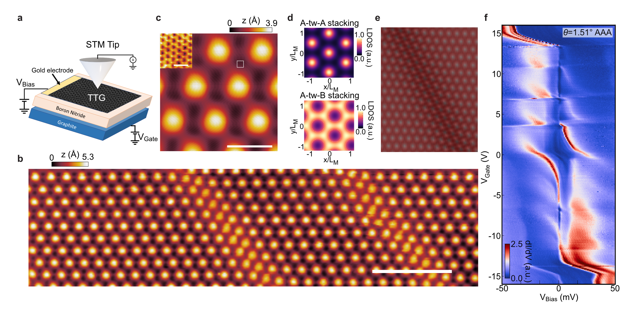
Fig. 1: Topography and spectroscopy of MATTG at zero magnetic field. a, Schematics of the STM experiment. MATTG is placed on an hexagonal Boron Nitride (hBN) substrate and doping is controlled by a graphite back gate. b, $290$ nm by $80$ nm area where two stripes separated by approximately $100$ nm are observed (tunneling set point parameters: $V_{\mathrm{{Bias}}}=100$ mV, $I=20$ pA; scale bar 50 nm). c, $26$ nm by $26$ nm topography showing moiré lattices with corresponding moire length of approximately $9$ nm (scale bar $10$ nm). The inset shows the atomic-scale hexagonal lattice of carbon atoms (scale bar $0.5$ nm). d, Calculated local density of states (LDOS) at charge neutrality originating from the bands within approximately $\pm 50$ meV energy window for A-tw-A (upper panel) and A-tw-B (lower panel) stacking. While in principle various configurations could arise, the A-tw-A stacking, where first and third layers are aligned, is seen experimentally. The peaks in LDOS correspond to AAA stacked regions where carbon atoms from three graphene layers are aligned. e, Simulated atomic distribution of MATTG with the first and third layers strained with respect to each other (See Methods, section 3 for simulation details). f, Tunneling conductance ($dI/dV$) spectroscopy as a function of $V_{\mathrm{Gate}}$ at twist angle $\theta=1.51\degree$ on an AAA site at $T=400$ mK. Clear signatures of symmetry breaking cascades, similar to twisted gaphene bilayers^{12, 13}, are observed.

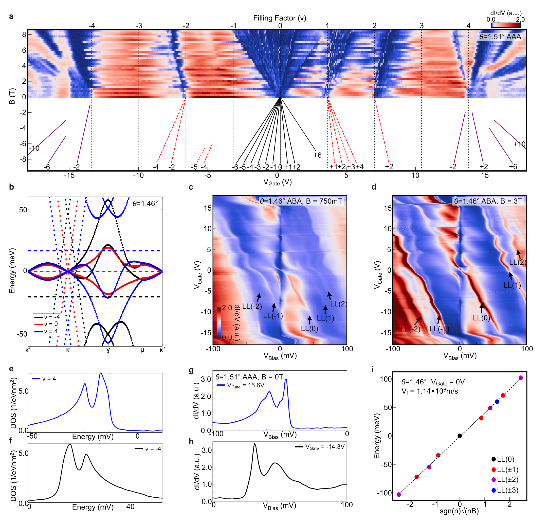
Fig. 2: LDOS Landau fan diagram and doping-dependent band deformations in MATTG. a, LDOS Landau fan diagram¹³ measured on an AAA site. The negative magnetic field fan shows the corresponding schematic of gaps between LLs emanating from the CNP (black); gaps emanating from non-zero integer fillings (red); and gaps between LLs from the dispersive bands (purple). b, Calculated MATTG band structure taking into account Hartree corrections. Horizontal dashed lines represent the positions of the Fermi levels at each doping. Electron (hole) doping shifts the Dirac-like band towards negative (positive) energy relative to the flat band (see also Methods, section 4). c, d, Point spectroscopy on an ABA site (in between AAA sites) at finite magnetic fields $B=0.75~{}\text{T}$ (c) and $B=3~{}\text{T}$ (d). Black arrows indicate LLs identified to originate from the additional Dirac cones characteristic of MATTG. e, f, Calculated density of states with Hartree corrections at $\nu=4$ (e) and $\nu=-4$ (f) for $\theta=1.51\degree$ at $B=0~{}\text{T}$. g, h, Point spectra taken at an AAA site at $B=0~{}\text{T}$ near $\nu=4$ ($V_{\rm Gate}=15.6~{}\text{V}$, g) and $\nu=-4$ ($V_{\mathrm{Gate}}=-14.3~{}\text{V}$, h). Note the asymmetric profile as expected from (e, f). i, Energies of LLs extracted from (c, d) at $V_{\mathrm{Gate}}=0$ V and plotted versus ${\rm sgn}(n)\sqrt{|n|B}$, with $n$ is the LL index, showing agreement with expectations from a Dirac dispersion. All data in this figure are taken within a $100\times 100$ nm² MATTG area with average $\theta=1.48\pm 0.03\degree$. The angles shown in the panels are obtained from measuring the exact distances between the closest AAA sites. Measurements are taken at $T=2~{}\text{K}$.

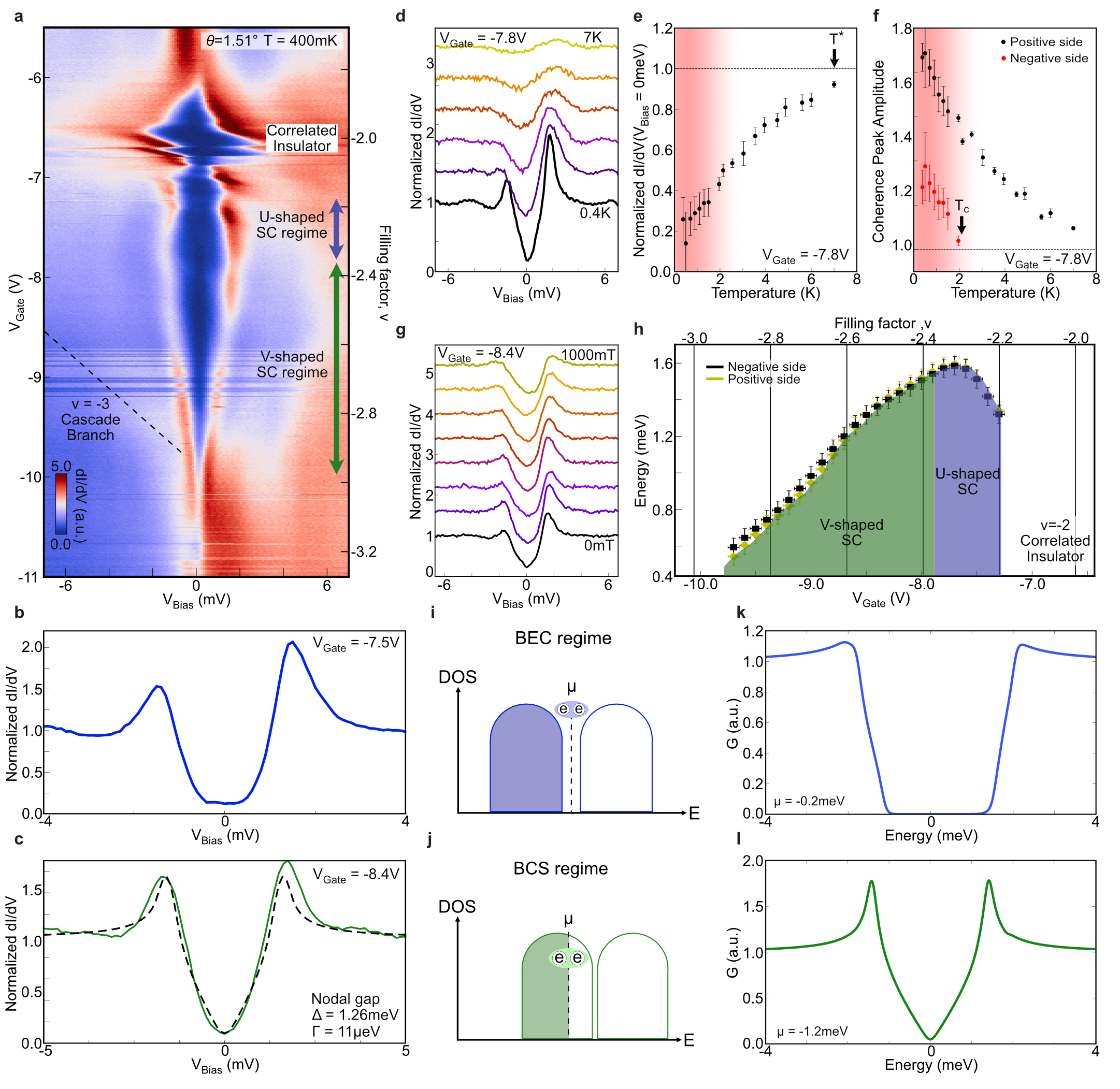
Fig. 3: Spectroscopic gap in the $\mathbf{-3<\nu<-2}$ range and signatures of unconventional superconductivity. a, Spectra near an AAA site (same area as Fig. 2a). Purple and green arrows denote $\nu$ range over which U- and V-shaped tunneling spectra, accompanied by clear coherence peaks, are observed. b, c, Normalized spectra showing U-shaped (b) and V-shaped (c) tunneling suppression. The data are normalized by a polynomial background, and fit to the Dynes formula (c) with a nodal superconducting order parameter (see Methods, section 5). d, Temperature dependence of the spectrum (lines correspond to $T=0.4,2,3,4.5,5.6,7$ K). e, Normalized zero-bias conductance vs. temperature; $T^{*}$ indicates the temperature at which the zero-bias conductance reaches 90% of the conductance outside the gap. f, Coherence-peak amplitude vs. temperature from normalized spectra on the electron (black) and hole (red) side. The hole-side coherence peak gets fully suppressed around $T_{c}\approx 2-2.5$ K. (d-f) are from the same dataset as Extended Data Fig. 5h-k. g, Magnetic-field dependence of the spectrum (lines correspond to $B=0,100,200,300,400,600,800,1000$ mT), from the same dataset as Extended Data Fig. 5a-d. h, Gap size $\Delta$ vs. $\nu$ ($V_{\rm Gate}$) extracted from (a) separately for electron (yellow) and hole (black) side coherence peaks. Color coding of different regions matches (a). i-l, Proposed BEC-BCS transition (i, j) mechanism that qualitatively reproduces U- and V-shaped spectra (k, l); see main text and Methods, section 6.2.

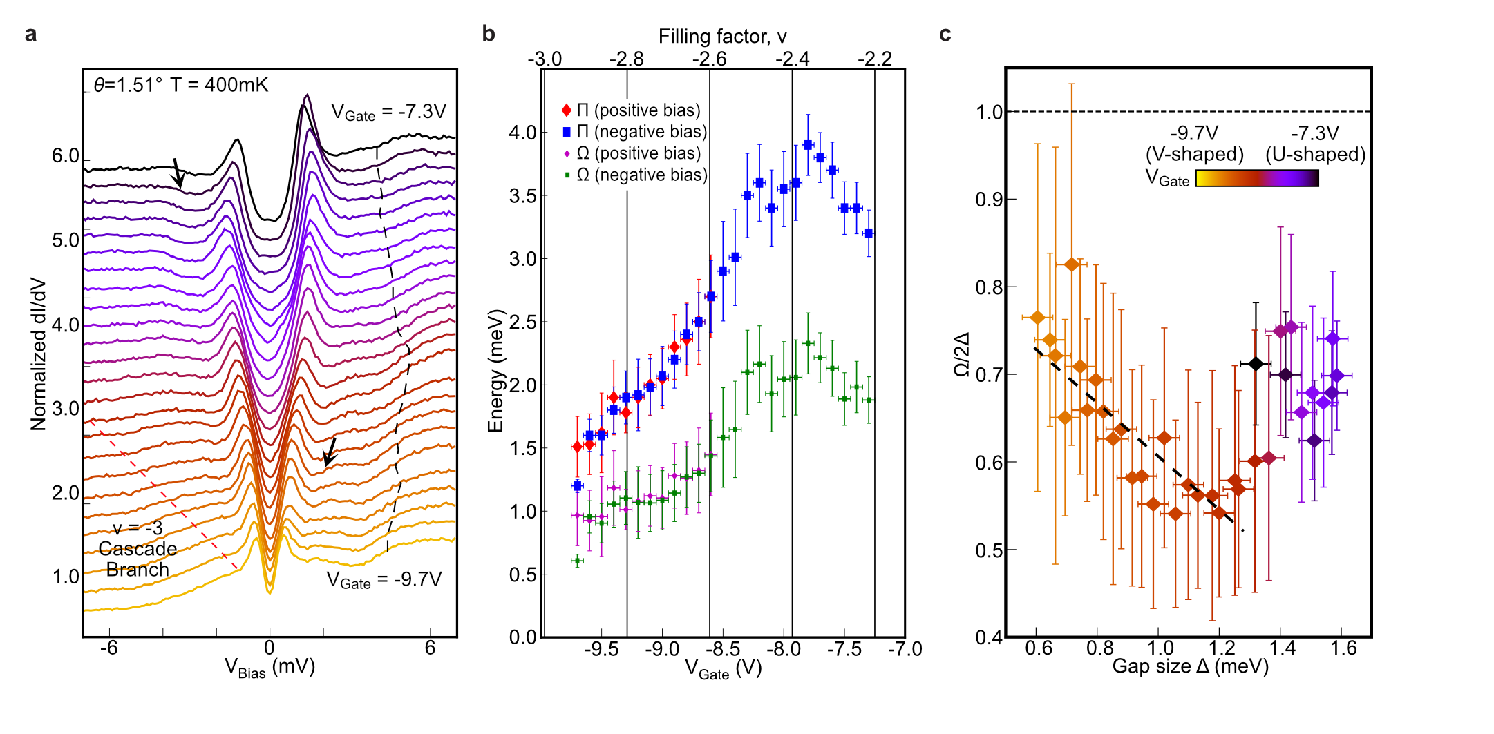
Fig. 4: Peak-dip-hump structure in MATTG. a, Line traces showing point spectra for $V_{\rm Gate}$ ranging from $-9.7$ V to $-7.3$ V (same dataset as Fig. 3a). Each spectrum is divided by the mean value for clarity. Red dashed line indicates the LDOS peak originating from the sub-band that abruptly shifts due to the cascade near $\nu=-3$; black dashed line indicates the shoulder of the upper flat band VHS. Black arrows denote the position of hole-side and electron-side dip-hump structure identified from the local minimum/maximum in $d^{2}I/dV^{2}$. b, Extracted energy $\Pi$ of the electron-side (red) and hole-side (blue) dip-hump structure and corresponding energy $\Omega$ of the bosonic mode on the electron side (purple) and hole side (green) versus filling factor ($V_{\rm Gate})$. c, Ratio $\Omega/2\Delta$ plotted versus $\Delta$ for both electron- and hole-side bosonic excitations. The black dashed line is a linear regression of the data at $V_{\rm Gate}$ ranging from $-9.7~{}\text{V}$ to $-8.6~{}\text{V}$ that shows anticorrelation of the two quantities for fillings at which V-shaped tunneling spectra are observed.

Methods:

1 Device fabrication

Similarly as in our previous STM measurements^{8, 13, 16} the device is fabricated using the Polydimethylsiloxane (PDMS)-assisted stack-and-flip technique using $\sim$30nm hBN and monolayer graphene. The flakes are exfoliated on SiO₂ and identified optically. We use a poly(bisphenol A carbonate) (PC)/PDMS stamp to pick up hBN at 90$\degree$C, and tear and twist graphene layers at 40$\degree$C. The PC film with the stack is then peeled off and transferred onto another clean PDMS, with MATTG side facing the PDMS. The PC film is dissolved in N-Methyl-2-pyrrolidone (NMP), followed by cleaning with Isopropyl alcohol (IPA). We kept the final PDMS in vacuum for several days. The stack on it is then transferred onto a chip with a graphite back gate and gold electrodes. Finally, MATTG is connected to the electrodes by another graphite flake.

2 STM measurements

The STM measurements were performed in a Unisoku USM 1300J STM/AFM system using a Platinum/Iridium (Pt/Ir) tip as in our previous works on bilayers^{8, 13, 16}. All reported features are observed with many (more than ten) different microtips. Unless specified otherwise, the parameters for $dI/dV$ spectroscopy measurements were $V_{\rm Bias}=100$ mV and $I=1$ nA, and the lock-in parameters were modulation voltage $V_{\rm mod}=0.2-1$ mV and frequency $f=973$ Hz. The piezo scanner is calibrated on a Pb(110) crystal by matching the lattice constant and verified by measuring the distance between carbon atoms. The twist-angle uncertainty is approximately $\pm 0.01\degree$, and determined by measuring moiré wavelengths from topography. Filling factor assignment has been performed by taking Landau fan diagrams as discussed previously¹³.

3 Stripe simulation

As mentioned in the main text, the stripes are believed to arise out of the restructuring of the moiré lattice. The flat-band scenario of interest arises when the top and bottom monolayers are AA stacked—all carbon atoms vertically aligned—while the middle layer is rotated by a twist angle $\sim 1.5^{\circ}$. While this situation seems understandably difficult to achieve during fabrication, it was shown in Ref. 6 that the desired AA stacking of the top and bottom is the energetically preferred configuration, and we therefore expect the system to relax into this configuration across large regions of the sample. This expectation is borne out by the observation of flat bands as well as the presence of a single moiré lattice constant as seen in STM.

There are two primary features in Fig. 1b that we wish to reproduce. The first, and most prominent, is the stripe, which can be obtained as follows. We let $\boldsymbol{a}_{1}=a(0,1)$ and $\boldsymbol{a}_{2}=a(-\sqrt{3}/2,-1/2)$ denote the Bravais primitive vectors of the graphene monolayer, where $a\approx 0.246\,\mathrm{\text{nm}}$ is the graphene lattice constant, and let $R(\phi)=e^{-i\phi\sigma^{y}}$ be a matrix that rotates by angle $\phi$. The bottom and middle lattices are simulated by plotting points at $\Lambda_{\mathrm{bot}}=\big{\{}R(-\theta/2)\big{(}n_{1}\boldsymbol{a}_{1}+n_{2}\boldsymbol{a}_{2}\big{)},n_{1,2}\in\mathbb{Z}\big{\}}$ and $\Lambda_{\mathrm{mid}}=\big{\{}R(\theta/2)\big{(}n_{1}\boldsymbol{a}_{1}+n_{2}\boldsymbol{a}_{2}\big{)},n_{1,2}\in\mathbb{Z}\big{\}}$. The stripe is then entirely determined by strain in the top layer, where the points plotted are instead $\Lambda_{\mathrm{top}}=\big{\{}R(-\theta/2)\big{(}n_{1}\boldsymbol{a}_{1}+n_{2}\boldsymbol{a}_{2}+f_{w}(-\frac{1}{2}n_{1}+n_{2})\boldsymbol{v}\big{)},n_{1,2}\in\mathbb{Z}\big{\}}$ where $f_{w}(x)=\frac{1}{\pi}{\arctan}(2x/w)+\frac{1}{2}$ and $\boldsymbol{v}=m_{1}\boldsymbol{a}_{1}+m_{2}\boldsymbol{a}_{2}$, $m_{1,2}\in\mathbb{Z}$ is a Bravais lattice vector. The function $f_{w}(x)$ is essentially a smoothened step function in that it interpolates between 0 and 1: $\lim_{x\to-\infty}f_{w}(x)=0$ and $\lim_{x\to+\infty}f_{w}(x)=1$. The size of the intermediate regime and hence the stripe width is determined by the parameter $w>0$, with $\lim_{w\to 0}f_{w}(x)=\Theta(x)$, the Heaviside function. In our definition of $\Lambda_{\mathrm{top}}$, we chose to have $f_{w}$ as a function $-\frac{1}{2}n_{1}+n_{2}$ since it results in a stripe along the $(-1/2,\sqrt{3}/2)$ direction and thus well represents the stripes shown in Fig. 1b. Putting these pieces together, one can see that in both regions where $\left|-\frac{1}{2}n_{1}+n_{2}\right|$ is large, the lattice points of $\Lambda_{\mathrm{bot}}$ and $\Lambda_{\mathrm{top}}$ should be directly above one another. In the region $-w/2\lesssim-\frac{1}{2}n_{1}+n_{2}\lesssim w/2$, the registry of the top and bottom layers changes from AA to AB and then back to AA.

The procedure detailed above yields a stripe, but does not account for a second feature of Fig. 1b: the moiré lattices on either side of the stripe are offset by about half of a moiré unit cell in the vertical ($\hat{{\boldsymbol{y}}}$) direction, which corresponds to a displacement of ${\boldsymbol{D}}_{\mathrm{shift}}=\frac{\sqrt{3}}{2}L_{M}\hat{{\boldsymbol{y}}}$, $L_{M}=a/\big{(}2\sin(\theta/2)\big{)}$. This offset at the moiré lattice scale is a result of a shift of the top and bottom lattices relative to the middle lattice occurring at the level of the microscopic scale of monolayer graphene. In particular, displacing the top and bottom layers by ${\boldsymbol{v}}_{\mathrm{shift}}\approx\theta\hat{{\boldsymbol{z}}}\times{\boldsymbol{D}}_{\mathrm{shift}}\approx-\frac{\sqrt{3}}{2}a\hat{{\boldsymbol{x}}}$ moves the moiré lattice by ${\boldsymbol{D}}_{\mathrm{shift}}$. Such a shift is readily implemented numerically by replacing the lattices $\Lambda_{\mathrm{bot}}$ and $\Lambda_{\mathrm{top}}$ with $\Lambda_{\mathrm{bot}}^{\prime}=\big{\{}R(-\theta/2)\big{(}n_{1}\boldsymbol{a}_{1}+n_{2}\boldsymbol{a}_{2}+f_{w}(-\frac{1}{2}n_{1}+n_{2})\boldsymbol{v}_{\mathrm{shift}}\big{)},n_{1,2}\in\mathbb{Z}\big{\}}$ and $\Lambda_{\mathrm{top}}^{\prime}=\big{\{}R(-\theta/2)\big{(}n_{1}\boldsymbol{a}_{1}+n_{2}\boldsymbol{a}_{2}+f_{w}(-\frac{1}{2}n_{1}+n_{2})(\boldsymbol{v}+{\boldsymbol{v}}_{\mathrm{shift}})\big{)},n_{1,2}\in\mathbb{Z}\big{\}}$. The middle layer is defined through $\Lambda_{\mathrm{mid}}$ as in the previous paragraph. For ease of visualization, $\Lambda_{\mathrm{top}}^{\prime}$ and $\Lambda_{\mathrm{bot}}^{\prime}$ are plotted in black while $\Lambda_{\mathrm{mid}}$ is plotted in red.

We emphasize that the primary purpose of this calculation is to reproduce the stripe in the simplest possible manner. A more complete study requires understanding the energetics, which would not only be needed to predict that width of the stripe (here, simply an input parameter), but which would also result in lattice relaxation within a unit cell.

4 Continuum model and Interaction-driven band structure renormalization

4.1 Continnum model

In this section, we summarize the continuum model^{3, 6} used to capture the low-energy theory of twisted trilayer graphene. In particular, we consider the case where the top and bottom layers are directly atop one another (AA stacked) and twisted by $-\theta/2$, while the middle layer is twisted by $+\theta/2$. The electronic structure of MATTG is obtained by an extension³ of the continuum model developed originally for twisted bilayer graphene (TBG)⁵⁴. As in that case, there are two independent sectors in the non-interacting limit distinguished by the valley $K$ and $K^{\prime}$. Without loss of generality, we therefore focus on valley $K$ in this section; the model relevant to valley $K^{\prime}$ may be obtained in a straightforward manner through time reversal. We let $\psi_{t}$, $\psi_{m}$, and $\psi_{b}$ denote the spinors one obtains by expanding the dispersion of monolayer graphene about valley $K$ for the top, middle and bottom layers, respectively. In terms of the microscopic operators of the graphene monolayers, that means $\psi_{\ell}({\boldsymbol{k}})=f_{\ell}({\boldsymbol{k}}+{\boldsymbol{K}}_{\ell})$, $\ell=t,m,b$. Importantly, as a result of the twist, the $K$ points of the different layers are not the same. The model is composed of a ‘diagonal’ Dirac piece and an ‘off-diagonal’ tunneling piece accounting for the moiré interlayer coupling: $H_{\mathrm{cont}}=H_{D}+H_{\mathrm{tun}}$. The Dirac term is broken up into three components, one for each layer, with $H_{D}=H_{t}+H_{m}+H_{b}$ where

$$H_{\ell} =\int_{\boldsymbol{k}}\psi^{\dagger}_{\ell}({\boldsymbol{k}})h_{\theta_{\ell}}({\boldsymbol{k}})\psi_{\ell}({\boldsymbol{k}}), h_{\theta_{\ell}}({\boldsymbol{k}}) =-v_{0}e^{i\theta_{\ell}\sigma^{z}/2}\big{(}k_{x}\sigma^{x}+k_{y}\sigma^{y}\big{)}e^{-i\theta_{\ell}/2}.$$ (1)

Above, $\ell=t,m,b$ identifies the layers, $v_{0}\sim 10^{6}\,\mathrm{\text{m/s}}$ is the Fermi velocity of the Dirac cones of monolayer layer graphene, and $\sigma^{x,y,z}$ are Pauli matrices acting on the A/B sublattice indices of the spinors $\psi_{\ell}$. The angle $\theta_{\ell}$ indicates the angle by which each layer is rotated, with $\theta_{t}=\theta_{b}=-\theta/2$ and $\theta_{m}=+\theta/2$. The magic angle for this model occurs for $\theta\approx 1.5^{\circ}$, which is related to the magic angle of TBG through a prefactor of $\sqrt{2}$: $\theta=1.5^{\circ}\approx\sqrt{2}\times 1.05^{\circ}$. The origins of this relation trace back to a similarity transformation that maps the MATTG continuum model into one of a decoupled TBG-like band structure with an interlayer coupling (to be discussed) multiplied by $\sqrt{2}$ and a graphene-like Dirac cone. We refer to Ref. 3 for an in-depth explanation of this relation.

We assume that tunneling only occurs between adjacent layers:

$$H_{\mathrm{tun}} =\sum_{j=1,2,3}\int_{\boldsymbol{k}}\Big{(}\psi^{\dagger}_{t}({\boldsymbol{k}})+\psi^{\dagger}_{b}({\boldsymbol{k}})\Big{)}T_{j}\psi_{m}({\boldsymbol{k}}+{\boldsymbol{q}}_{j})+h.c.,$$ (2)

where the momenta shift and the tunneling matrices are given by

$${\boldsymbol{q}}_{j} =\frac{4\pi}{3L_{M}}R\left(\frac{2\pi}{3}(j-1)\right)\begin{pmatrix}0\\ -1\end{pmatrix},$$

$$T_{j} =w_{0}+w_{1}\left(e^{-2\pi(j-1)i/3}\sigma^{+}+e^{2\pi(j-1)i/3}\sigma^{-}\right)$$ (3)

with $R(\phi)=e^{-i\phi\sigma^{y}}$ is a $2\times 2$ matrix acting on vector indices, $L_{M}=a/[2\sin(\theta/2)]$, and $\sigma^{\pm}=(\sigma^{x}\pm i\sigma^{y})/2$. The tunneling strength is determined by the parameters $w_{0}$ and $w_{1}$; in this paper we set $(w_{0},w_{1})=(55,105)\,\mathrm{\text{meV}}$. (Note that the conventions used in this section are rotated by 90^∘ relative to those of section 3.)

This model possesses a number of symmetries. We have already alluded to time reversal, with which one may obtain the continuum model Hamiltonian corresponding to the valley $K^{\prime}=-K$. We therefore re-introduce a valley label, writing $\psi_{\ell}\to\psi_{v,\ell}$ with $v=K,K^{\prime}$. A number of spatial symmetries are also present in this model, but for our purposes it is sufficient to note that the model is invariant under rotations by $60^{\circ}$, under which the spinors transform as $\psi_{\ell}({\boldsymbol{k}})\to\tau^{x}\sigma^{x}e^{2\pi i\tau^{z}\sigma^{z}/3}\psi_{\ell}\big{(}R(2\pi/6){\boldsymbol{k}}\big{)}$, where $\tau^{x,y,z}$ are Pauli matrices acting on the (now suppressed) valley indices.

To diagonalize the continuum model, we recall that the spinor operators $\psi_{\ell}$ are not all defined about a common momentum point. Hence the tunneling term in Eq. (2) does not involve a momentum exchange of ${\boldsymbol{q}}_{j}$, but rather $K_{t}=K_{b}=K_{m}+{\boldsymbol{q}}_{j}$ and $K_{t}^{\prime}=K_{b}^{\prime}=K_{m}-{\boldsymbol{q}}_{j}$, which differ by a moiré reciprocal lattice vector. We therefore define operators $\Psi_{v,\ell}$ about a common momentum point for each valley through $\Psi_{v,t/b}({\boldsymbol{k}})=\psi_{v,t/b}({\boldsymbol{k}})$ and $\Psi_{K/K^{\prime},m}({\boldsymbol{k}})=\psi_{K/K^{\prime},m}({\boldsymbol{k}}\pm{\boldsymbol{q}}_{1})$, where the $+$ ($-$) corresponds to $K$ ($K^{\prime}$) (the choice ${\boldsymbol{q}}_{1}$ is arbitrary—${\boldsymbol{q}}_{2}$ and ${\boldsymbol{q}}_{3}$ could be equally chosen). Grouping the valley, layer, sublattice, and spin labels into a single indice, $\Psi_{\alpha}$, we can express $H_{\mathrm{cont}}$ in matrix form as

$$H_{\mathrm{cont}} =\sum_{{\boldsymbol{G}},{\boldsymbol{G}}^{\prime}}\int_{{\boldsymbol{k}}\in\mathrm{mBZ}}\Psi^{\dagger}_{\alpha}({\boldsymbol{k}}+{\boldsymbol{G}})h^{(\mathrm{cont})}_{\alpha,{\boldsymbol{G}};\alpha^{\prime},{\boldsymbol{G}}^{\prime}}({\boldsymbol{k}})\Psi_{\alpha^{\prime}}({\boldsymbol{k}}+{\boldsymbol{G}}^{\prime});$$ (4)

${\boldsymbol{G}}$ and ${\boldsymbol{G}}^{\prime}$ are moiré reciprocal lattice vectors defined via ${\boldsymbol{G}}=n_{1}\boldsymbol{\mathcal{G}}_{1}+n_{2}\boldsymbol{\mathcal{G}}_{2}$, $n_{1,2}\in\mathbb{Z}$ where $\boldsymbol{\mathcal{G}}_{1}={\boldsymbol{q}}_{2}-{\boldsymbol{q}}_{1}$ and $\boldsymbol{\mathcal{G}}_{2}={\boldsymbol{q}}_{3}-{\boldsymbol{q}}_{1}$. The integration over ${\boldsymbol{k}}$ includes only those momenta within the moiré Brillouin zone (mBZ).

4.2 Interaction-driven band structure renormalization

The presence of flat bands in MATTG necessitates the consideration of interaction-driven band structure corrections. As demonstrated experimentally in our previous work on twisted graphene bilayers¹⁶, filling-dependent interaction effects, specifically Hartree and Fock corrections, drastically alter the electron dispersion. Here we incorporate only a Hartree mechanism^{17, 18, 19, 20} in the analysis. In TBG we found¹⁶ that the main role of the Fock correction, provided that one does not consider the nature of the correlated states and the cascade, is to broaden the band structure at the charge neutrality point ($\nu=0$) and to counteract band inversions at the zone center promoted by Hartree effects. For comparison with the experiment presented in Fig. 2, where we focus only on $\nu=\pm 4$, we can thus ignore Fock corrections as a first approximation. Similar Hartree-driven band structure renormalizations were considered recently in the literature^{14, 15}, and our analysis together with the experimental results are consistent with their conclusions.

We introduce Coulomb interaction into the system through

$$H_{C} =\frac{1}{2}\int d^{2}{\boldsymbol{r}}\,d^{2}{\boldsymbol{r}}^{\prime}\,\delta\rho({\boldsymbol{r}})V({\boldsymbol{r}}-{\boldsymbol{r}}^{\prime})\delta\rho({\boldsymbol{r}}^{\prime}).$$ (5)

Here, $V({\boldsymbol{r}})=e^{2}/(4\pi\epsilon|{\boldsymbol{r}}|)$ is the Coulomb potential and $\delta\rho({\boldsymbol{r}})=\Psi^{\dagger}({\boldsymbol{r}})\Psi({\boldsymbol{r}})-\rho_{\mathrm{CN}}({\boldsymbol{r}})$, where $\rho_{\mathrm{CN}}({\boldsymbol{r}})=\langle\Psi^{\dagger}({\boldsymbol{r}})\Psi({\boldsymbol{r}})\rangle_{\mathrm{CN}}$ is the expectation value of the density at the charge neutrality point. The use of $\delta\rho({\boldsymbol{r}})$ instead of $\rho({\boldsymbol{r}})$ in the interaction is motivated by the expectation that the input parameters of the model $H_{\mathrm{cont}}$ already include the effect of interactions at the charge neutrality point. Although numerically expedient, this assumption is not strictly correct since the input parameters in actuality refer to three independent graphene monolayers. Nevertheless, for the purpose of making qualitative comparisons with Fig. 2, we do not expect this distinction to be important. The dielectric constant $\epsilon$ in the definition of $V({\boldsymbol{r}})$ is used as a fitting parameter; see section 4.3 for details.

We study the effect of the interacting continuum model of MATTG through a self-consistent Hartree mean-field calculation. Instead of solving the many-body problem, we obtain the quadratic Hamiltonian that best approximates the full model when only the symmetric contributions of $H_{C}$ are included, i.e., the Fock term is neglected as explained above. Thus instead of $H_{\mathrm{cont}}+H_{C}$, we study the Hamiltonian

$$H_{\mathrm{MF}}^{(\nu)} =H_{\mathrm{cont}}+H^{(\nu)}_{\mathrm{H}}-\frac{1}{2}\langle H_{\mathrm{H}}^{(\nu)}\rangle_{\nu},$$ (6)

where $H_{\mathrm{H}}^{(\nu)}$ is the Hartree term at filling $\nu$,

$$H_{\mathrm{H}}^{(\nu)} =\int_{{\boldsymbol{k}},{\boldsymbol{k}}^{\prime},{\boldsymbol{q}}}V({\boldsymbol{q}})\langle\Psi^{\dagger}({\boldsymbol{k}}^{\prime}+{\boldsymbol{q}})\Psi({\boldsymbol{k}}^{\prime})\rangle_{\nu}\Psi^{\dagger}({\boldsymbol{k}})\Psi({\boldsymbol{k}}-{\boldsymbol{q}}),$$ (7)

and the last term in Eq. (6) simply ensures there is no double counting when one calculates the total energy. In the above equation, $V({\boldsymbol{q}})=2\pi e^{2}/(\epsilon|{\boldsymbol{q}}|)$ is the Fourier transform of the Coulomb interaction $V({\boldsymbol{r}})$ in Eq. (5), and the expectation value $\langle\hat{\mathcal{O}}\rangle_{\nu}=\langle\hat{\mathcal{O}}\rangle_{\mathrm{occ}}-\langle\hat{\mathcal{O}}\rangle_{\mathrm{CN}}$ only includes states that are filled up to $\nu$ relative to charge neutrality, as defined by diagonalizing the Hamiltonian $H_{\mathrm{MF}}^{(\nu)}$. Typically, for a “jellium”-like model, the expectation value vanishes save for ${\boldsymbol{q}}=0$, which is subsequently cancelled by the background charge—allowing one to set $V({\boldsymbol{q}}=0)=0$ and completely ignore the Hartree interaction. However, because the moiré pattern breaks continuous translation symmetry, momentum is only conserved modulo a reciprocal lattice vector. We therefore obtain

$$H_{\mathrm{H}}^{(\nu)} =\sum_{{\boldsymbol{G}}}^{\prime}V({\boldsymbol{G}})\int_{{\boldsymbol{k}}^{\prime}}\langle\Psi^{\dagger}({\boldsymbol{k}}^{\prime}+{\boldsymbol{G}})\Psi({\boldsymbol{k}}^{\prime})\rangle_{\nu}\int_{{\boldsymbol{k}}}\Psi^{\dagger}({\boldsymbol{k}})\Psi({\boldsymbol{k}}-{\boldsymbol{G}}),$$ (8)

where the prime above the summation over the moiré reciprocal lattice vectors indicates that ${\boldsymbol{G}}=0$ is excluded. The self-consistent procedure begins by assuming some initial value of $H_{\mathrm{H}}^{(\nu)}$ and diagonalizing the corresponding mean-field Hamiltonian $H_{\mathrm{MF}}^{(\nu)}$ to obtain the Bloch wavefunctions and energy eigenvalues. These quantities are then used re-compute the expectation values that define $H_{\mathrm{H}}^{(\nu)}$ and thus $H_{\mathrm{MF}}^{(\nu)}$. This process is repeated until one obtains the quadratic Hamiltonian $H_{\mathrm{MF}}^{(\nu)}$ that yields the correlation functions $\langle\cdot\rangle_{\nu}$ used in its definition.

It has further been shown^{17, 55} that the Hartree potential is dominated by the first ‘star’ of moiré reciprocal lattice vectors, which in our conventions corresponds to ${\boldsymbol{G}}_{n}=R\big{(}2\pi(n-1)/6\big{)}\frac{4\pi}{\sqrt{3}L_{M}}(1,0)^{T}$ for $n=1,\dots,6$, with $R(\phi)$ a rotation matrix. In this last approximation that we employ, the $2\pi/6$ rotation symmetry of the continuum model greatly simplifies the calculation of the Hartree term. Notably, $V({\boldsymbol{G}})\int_{{\boldsymbol{k}}^{\prime}}\langle\Psi^{\dagger}({\boldsymbol{k}}^{\prime}+{\boldsymbol{G}})\Psi({\boldsymbol{k}}^{\prime})\rangle_{\nu}$ must be the same for all ${\boldsymbol{G}}_{n}$, and, instead of Eq. (8), we use

$$H_{\mathrm{H}}^{(\nu)} =V_{\mathrm{H}}^{(\nu)}\sum_{n=1}^{6}\int_{\boldsymbol{k}}\Psi^{\dagger}({\boldsymbol{k}})\Psi({\boldsymbol{k}}-{\boldsymbol{G}}_{n}), V_{\mathrm{H}}^{(\nu)} =\frac{1}{6}\sum_{n=1}^{6}V({\boldsymbol{G}}_{n})\int_{{\boldsymbol{k}}^{\prime}}\langle\Psi^{\dagger}({\boldsymbol{k}}^{\prime}+{\boldsymbol{G}})\Psi({\boldsymbol{k}}^{\prime})\rangle_{\nu}\,.$$ (9)

The self-consistent procedure in this case is identical to that described in the previous paragraph, but due to the reduced number of reciprocal lattice vectors that are included in the summation the calculation is computationally easier. Convergence is typically reached within $\sim 6$ iterations.

For clarity, all bands corresponding to different fillings plotted in Fig. 2b have been shifted so that the Dirac points of the flat bands always occur at the zero of the energy scale; it follows that the (independent) graphene-like Dirac cone is then displaced in energy relative to the fixed reference point of the flat bands for each filling. If this procedure was not performed for clarity purposes, then the Hartree calculation would yield band structures with a graphene-like Dirac cone fixed at one energy for all fillings, but with shifted flat bands relative to it, as predicted in ab-initio calculations¹⁴.

4.3 Hartree correction and estimate of dielectric constant

As discussed in the previous section, due to Hartree corrections, the Dirac cones shift downwards (upwards) in energy relative to the flat bands under electron (hole) doping, as seen in Fig. 2b-d. These relative shifts are measured to be rather large ($\approx 70\,\mathrm{\text{meV}}$ for $\nu=+4$ and $\approx 50\,\mathrm{\text{meV}}$ for $\nu=-4$), similar to the bandwidth of the MATTG flat bands (approximately $50$ meV). These relative shifts allow us to estimate an effective dielectric constant $\epsilon$ to be used in Hartree band-structure-renormalization calculations. In particular, we find that $\epsilon=12-13$ quantitatively reproduces the observed Dirac point shifts at $\nu=\pm 4$. Finally, we note that the relative shift between Dirac cones and flat bands may also explain a certain discrepancy between our measurements and the bandwidth estimates of the flat bands found in transport¹ that assumed fixed relative position between Dirac point and flat points. This assumption, neglecting the Hartree correction leads to an overestimate of a bandwidth by a factor of $\sim 2$ (we measure flat band width to be approximately $50$ meV while Ref. 1 found it to be around $100$ meV).

5 Tunneling conductance normalization and fitting procedure

In Fig. 3b,c the tunneling conductance has been normalized by dividing the spectra with a sixth-order polynomial fit that preserves the area of the spectrum ⁵⁶ (see also Extended Data Fig. 9). This procedure returns normalized dI/dV curves that approach unity outside of the spectroscopic gap and removes in part the large asymmetry between electrons and holes near $\nu=-2$ and above $V_{\rm Bias}=5$ meV. We emphasize that the regimes displaying U- and V-shaped tunneling spectra are clearly visible both before and after this normalization procedure. The dip-hump structure persists after this step as well (see black arrow in Extended Data Fig. 9).

The normalized dI/dV curves are fitted with the Dynes formula²⁶,

$$\frac{dI}{dV}\propto\int_{-\infty}^{\infty}d\omega\int_{0}^{2\pi}d\theta~{}\mathrm{Re}\left[\frac{\omega+i\Gamma}{\sqrt{(\omega+i\Gamma)^{2}-\Delta(\theta)^{2}}}\right]\left.\left(-\frac{df}{d\omega}\right)\right\rvert_{\omega=\omega+eV}\,,$$ (10)

where $f(\omega)=1/(e^{\omega/k_{B}T}+1)$ ($k_{B}$ is a Boltzmann constant and $T=400$ mK in our measurements); $\Delta(\theta)$ is the superconducting pairing potential and; spectral broadening coming from disorder and finite lifetime of Cooper pairs are incorporated by the parameter $\Gamma$. We consider isotropic $s$-wave pairing, a pairing with a nodal order parameter, and a combination of the two (see also section 6 and Extended Data Fig. 7 for a more detailed discussion and fits). For the nodal case we use $\mathrm{\Delta}(\theta)=\Delta_{0}\cos(2\theta)$ (i.e., a $d$-wave profile), though any $\mathrm{\Delta}(\theta)=\Delta_{0}\cos(N\theta)$ with integer $N\neq 0$ gives the same spectrum. We therefore do not distinguish between different nodal order parameters, e.g., $p$- versus $d$- versus $f$-wave. In the plots, we also took into account the broadening due to finite lock-in modulation excitation $V_{\rm mod}=200\micro$ V.

6 Possible Scenarios of U-shaped to V-shaped spectral evolution

In the main text, we introduced the experimental observation that the tunneling conductance exhibits two qualitatively different tunneling profiles (U- vs. V-shaped) as a function of filling. We now discuss the details of two possible scenarios for this outcome: $(i)$ a BCS-like superconductor with filling-dependent order parameter symmetry and $(ii)$ a BEC-to-BCS transition with a common nodal order parameter. As noted in the main text, we emphasize that ‘BCS’ in this context does not imply any assumptions regarding the pairing mechanism or coupling strength, but simply refers to a pairing scenario wherein the chemical potential lies inside the band. Finally, we discuss the Ginzburg-Landau coherence length in the BEC-BCS transition scenario and argue that it is consistent with the results of Ref. 1.

6.1 BCS-like superconductor with filling-dependent order parameter symmetry

The existence of U- and V-shaped tunneling spectra suggests that superconductivity evolves with doping from a fully gapped to a gapless state. Here we address the possibility that these two regimes both arise from Cooper pairing a partially filled band with a Fermi surface, but with qualitatively different superconducting order parameters. This scenario a priori does not address the different behaviors of the Ginzburg-Landau coherence length $\xi_{\rm GL}$ seen in Ref. 1, e.g., the scaling of $\xi_{\rm GL}$ with the interparticle spacing (see section 6.2.2). Nevertheless, whatever mechanism underlies the putative change in order parameter could potentially conspire to yield such dependence.

The V-shaped spectra can be adequately fit by postulating a nodal order parameter, as described in the main text and in section 5. In the present scenario, the U-shaped spectra are best fit by invoking multiple co-existing order parameters: either an $s$-wave gap together with a nodal order parameter or a combination of two nodal order parameters (e.g., $d_{x^{2}-y^{2}}+id_{xy}$) that together produce a gap in the tunneling conductance. Extended Data Fig. 7e displays the relevant fits. As noted in the main text, a similar change in pairing order with doping has been proposed in cuprates²⁷ (albeit with a less pronounced U-to-V evolution). Moreover, it has been argued that have argued that a $d_{x^{2}-y^{2}}+id_{xy}$ spin-fluctuation-mediated pairing is energetically unfavourable compared to a real superposition of the two order parameters.¹⁴

6.2 BEC-to-BCS transition

6.2.1 Tunnelling current

To describe the tunneling current expected in the BEC-BCS transition scenario and demonstrate qualitative consistency with experiment, we consider a phenomenological two-parabolic-band model. Specifically, we model the system near filling $\nu=-2$ with two bands of energy (in these two sections we set $\hbar=1$)

$$\xi_{\pm,{\boldsymbol{k}}}=\pm\left(\frac{k^{2}}{2m}+\Delta_{\mathrm{CI}}\right)-\mu,$$ (11)

separated by a $2\Delta_{\mathrm{CI}}$ correlated-insulator gap. Each band admits a two-fold ‘spin’ degeneracy—which need not coincide exactly with physical spin, but could, e.g., represent some combination of spin and valley. In the absence of pairing, $\mu$ residing in the electron band $\xi_{+}$ (hole band $\xi_{-}$) corresponds to filling $\nu=-2+\delta n$ with $\delta n>0$ ($\delta n<0$). We focus primarily on the hole-doping case relevant for experiment.

For simplicity, we assume a ‘spin’-singlet, nodal $d$-wave pairing with a pair field $\Delta_{\boldsymbol{k}}$ that is the same in the electron and hole bands; inter-band pairing is neglected. (We anticipate that triplet pairing would yield similar results, as would other nodal order parameters.) The standard Bogoliubov–de Gennes formalism yields

$$E_{\pm,{\boldsymbol{k}}} =\sqrt{\xi_{\pm,{\boldsymbol{k}}}^{2}+\Delta_{{\boldsymbol{k}}}^{2}}\,, u_{\pm,{\boldsymbol{k}}}^{2} =1+\frac{\xi_{\pm,{\boldsymbol{k}}}}{E_{\pm,{\boldsymbol{k}}}}\,, v_{\pm,{\boldsymbol{k}}}^{2} =1-\frac{\xi_{\pm,{\boldsymbol{k}}}}{E_{\pm,{\boldsymbol{k}}}}$$ (12)

with $u_{\pm,{\boldsymbol{k}}}^{2},v_{\pm,{\boldsymbol{k}}}^{2}$ coherence factors describing overlap of the bare electron/hole wavefunctions with those of quasiparticles with dispersion $E_{\pm,{\boldsymbol{k}}}$. The BEC phase corresponds to $|\mu|<\Delta_{\mathrm{CI}}$. Here $\Delta_{\rm CI}$ renders the quasiparticles fully gapped despite the assumed nodal $d$-wave order parameter, and population of the electron and hole bands arises solely from pairing. (At $\mu=0$, the symmetry built into the electron and hole bands implies that the system remains undoped, corresponding to $\nu=-2$, even with $\Delta_{{\boldsymbol{k}}}\neq 0$.) The regime $|\mu|>\Delta_{\rm CI}$ corresponds to a BCS phase wherein an electron- or hole-like Fermi surface undergoes Cooper pairing, yielding gapless quasiparticle excitations due to nodes in $\Delta_{{\boldsymbol{k}}}$. Figure 3i,j schematically depicts the chemical potential associated with these two phases.

The tunneling current follows from

$$I(eV,\mu)\propto\sum_{s=\pm}\int d^{2}{\boldsymbol{k}}\,\left\{u_{s,{\boldsymbol{k}}}^{2}\big{[}f(E_{s,{\boldsymbol{k}}}-eV)-f(E_{s,{\boldsymbol{k}}})\big{]}-v_{s,{\boldsymbol{k}}}^{2}\big{[}1-f(-E_{s,{\boldsymbol{k}}}-eV)-f(E_{s,{\boldsymbol{k}}})\big{]}\right\},$$ (13)

where $f(E)=1/(e^{E/k_{B}T}+1)$ is the Fermi-Dirac distribution; the differential tunneling conductance $dI/dV$ is obtained by numerically differentiating the current after the integral is evaluated. Below we will use this general formula to evaluate the tunneling conductance across the BEC-BCS transition. As a primer, however, it is instructive to examine limiting cases.

Consider first the conductance deep in the BCS phase. Here the current simplifies dramatically for relevant voltages. First, focusing on the hole-doping case with $\mu\ll-\Delta_{\rm CI}$, we can neglect the electron band to an excellent approximation and focus solely on momenta near the Fermi surface for the hole band. The remaining quasiparticle dispersion $E_{-,{\boldsymbol{k}}}$ then has two ‘branches’ with the same energy—corresponding to excitations above and below the hole-like Fermi surface (i.e., with $\xi_{-,{\boldsymbol{k}}}>0$ and $\xi_{-,{\boldsymbol{k}}}<0$). That is, for each momentum $k^{+}>k_{F}$ ($k_{F}$ is the Fermi momentum), there exists a momentum $k^{-}<k_{F}$ such that $\xi_{-,{\boldsymbol{k}}^{+}}=-\xi_{-,{\boldsymbol{k}}^{-}}$, but $E_{-,{\boldsymbol{k}^{+}}}=E_{-,{\boldsymbol{k}^{-}}}$. The momentum-dependent part of the coherence factors therefore cancels, yielding a tunneling current

$$I(eV,\mu)\propto\int d^{2}{\boldsymbol{k}}\,\Big{\{}\big{[}f(E_{-,{\boldsymbol{k}}}-eV)-f(E_{-,{\boldsymbol{k}}})\big{]}-\big{[}1-f(-E_{-,{\boldsymbol{k}}}-eV)-f(E_{-,{\boldsymbol{k}}})\big{]}\Big{\}}$$ (14)

that depends on the quasiparticle dispersion but not the coherence factors. Upon taking $d^{2}{\boldsymbol{k}}\approx k_{F}dkd\theta$, carrying out a variable change $\omega=\sqrt{\xi_{-,{\boldsymbol{k}}}^{2}+\Delta_{{\boldsymbol{k}}}}$, and assuming no $|{\boldsymbol{k}}|$ dependence in the pairing gap evaluated at the Fermi surface [$\Delta_{{\boldsymbol{k}}}\rightarrow\Delta(\theta)$], we arrive at the conventional BCS expression:

$$I(eV,\mu) \propto\int_{0}^{2\pi}d\theta\int_{\Delta(\theta)}^{\infty}d\omega\frac{\omega}{\sqrt{\omega^{2}-\Delta(\theta)^{2}}}\Big{\{}\big{[}f(\omega-eV)-f(\omega)\big{]}-\big{[}1-f(-\omega-eV)-f(\omega)\big{]}\Big{\}}$$

$$\propto\int_{0}^{2\pi}d\theta\int_{\Delta(\theta)}^{\infty}d\omega\frac{\omega}{\sqrt{\omega^{2}-\Delta(\theta)^{2}}}\left(-\frac{df}{d\omega}eV\right)$$

$$\implies\frac{dI}{dV} \propto\int_{0}^{2\pi}d\theta\int_{\Delta(\theta)}^{\infty}d\omega\frac{\omega}{\sqrt{\omega^{2}-\Delta(\theta)^{2}}}\left(-\frac{df}{d\omega}\right).$$ (15)

Implementing the Dynes substitution²⁶ $\omega\to\omega+i\Gamma$ then recovers the expression from Eq. (10). The square-root factor in the denominator underlies coherence peaks associated with pairing-induced density-of-states rearrangement.

By contrast, in the BEC phase ($|\mu|<\Delta_{\rm CI}$), or sufficiently close to the BEC-BCS transition, the simplifying procedure above breaks down. Both electron and hole bands need to be retained; $\Delta_{{\boldsymbol{k}}}$ can not be simply evaluated at a Fermi surface, and hence dependence on the orientation and magnitude of ${\bf k}$ become important; and since the minimum of the quasiparticle dispersion $E_{\pm,{\boldsymbol{k}}}$ occurs at or near ${\boldsymbol{k}}=0$, the momentum-dependent part of the coherence factors no longer perfectly cancels. Together, these details manifest both through a “softening” of the coherence peaks in the tunneling conductance and the generation of a tunneling gap for any pairing function $\Delta_{{\boldsymbol{k}}}$, $d$-wave or otherwise, in the BEC state; cf. Fig. 3k,l.

Returning to the general current formula in Eq. (13), in simulations of Fig. 3k,l and supplemental simulations below, we employ a $d$-wave pairing potential with

$$\Delta_{{\boldsymbol{k}}}=\Delta_{0}h(k)\cos(2\theta).$$ (16)

Here $k$ and $\theta$ are the magnitude and polar angle of ${\boldsymbol{k}}$, while $\Delta_{0}$ sets the pairing energy scale. We take the $k$-dependent prefactor to be $h({k})=\mathrm{tanh}({k}^{2}\ell^{2})$, where $\ell$ is roughly the real-space distance over which the $d$-wave pairing potential acts. This choice results in $\Delta_{{\boldsymbol{k}}}$ vanishing at $k=0$ as required for $d$-wave pairing, and regularizes the unphysical divergence that would appear with a simple $h(k)\propto k^{2}$ profile in a manner that preserves locality in real-space. Let $\eta\equiv 2m\Delta_{0}\ell^{2}$ be a dimensionless quantity involving $\ell$. In the regime of the BCS phase with $k_{F}\ell\gg 1$, near the Fermi surface we have $\Delta_{{\boldsymbol{k}}}\approx\Delta_{0}\cos(2\theta)$; hence the value of $\eta$ is largely irrelevant provided $k_{F}^{2}/2m$ remains sufficiently large compared to $\Delta_{0}$. In both the BCS regime with $k_{F}\ell\lesssim 1$ and throughout the BEC phase, the choice of $\eta$ is more significant. Here, for the physically important ‘small’ momenta, the pairing behaves like $\Delta_{{\boldsymbol{k}}}\approx\Delta_{0}k^{2}\ell^{2}\cos(2\theta)$ and should be compared to the $k^{2}/2m$ kinetic energy scale. With $\eta\lesssim 1$, pairing effects are suppressed since the latter scale dominates over the former. By contrast, with $\eta\gtrsim 1$ the pairing scale dominates and correspondingly yields more dramatic signatures in density of states and tunneling conductance. In particular, the coherence peaks appear most prominently in the BEC phase at $\eta\gg 1$.

The tunneling conductance in the BEC and BCS phases can be studied as a function of chemical potential or as a function of filling. In our formalism, treating $\mu$ as the tuning parameter is more convenient since all $\mu$ dependence is contained in the quasiparticle dispersion $E_{\pm,{\boldsymbol{k}}}$ and the relation between filling and $\mu$ evolves nontrivially between the BEC and BCS phases. In experiment, however, the gate-controlled filling $\nu$ is the natural tuning parameter. Additionally, the pairing strength and $\nu=-2$ gap, modeled here by $\Delta_{0}$ and $\Delta_{\rm CI}$, certainly depend on $\nu$—which further complicates the relation between filling and $\mu$. We defer a careful examination of this relation to future work. Instead, here we will simply explore the tunneling conductance as a function of $\mu$, with $\mu$-dependent $\Delta_{0}$ and $\Delta_{\rm CI}$ input parameters extracted (crudely) from the experiment as follows.

First, for each filling we fix $\Delta_{0}$ to the measured location of coherence peaks in Fig. 3h (and linearly extrapolate to continue to more negative $\mu$ values). In the V-shaped regime this assignment is expected to be quantitatively reliable, given our interpretation of that regime as a BCS phase (which would indeed have coherence peaks set by $\Delta_{0}$). However, the U-shaped regime, interpreted as a BEC phase, would have coherence peaks at an energy determined by multiple parameters including $\mu,\Delta_{\rm CI}$, and $\Delta_{0}$; thus here the assignment becomes an approximation that we invoke for simplicity. We then obtain a $\Delta_{0}$ vs. $\mu$ profile by naively replacing filling (or gate voltage) with $\mu$; i.e., we ignore the nontrivial relation linking these quantities. To determine $\Delta_{\rm CI}$ vs. $\mu$, we first fix the value at $\mu=0$ to be $\Delta_{\rm CI,0}=2.7$ meV, corresponding to the $\nu=-2$ spectral gap seen in Extended Data Fig. 4. We also fix the chemical potential $\mu_{*}$ corresponding to the BEC-BCS transition, which in our model occurs when $-\mu_{*}=\Delta_{\rm CI}(\mu_{*})$. We specifically set $\mu_{*}=-0.8$ meV so that the transition coincides roughly with the experimentally observed U-to-V change in Fig. 3 (after replacing density as $\mu$ as described above). We phenomenologically model the remaining $\mu$ dependence of $\Delta_{\rm CI}$ as

$$\Delta_{\rm CI}(\mu)=\begin{cases}\Delta_{\rm CI,0}\frac{\gamma_{\rm CI}^{2}}{\mu^{2}+\gamma_{\rm CI}^{2}}&\mu\geq\mu_{*}\\ \alpha_{2}\mu^{2}+\alpha_{1}\mu+\alpha_{0}&\mu_{*}\geq\mu\end{cases}$$ (17)

with $\alpha_{2}=\Delta_{\rm CI}(\mu^{+})/(\mu_{*}-\mu_{**})^{2}$, $\alpha_{1}=-2\Delta_{\rm CI}(\mu^{+})\mu_{**}/(\mu_{*}-\mu_{**})^{2}$, $\alpha_{0}=\Delta_{\rm CI}(\mu^{+})\mu_{**}^{2}/(\mu_{*}-\mu_{**})^{2}$ and $\mu_{**}=-1.1$ meV. We further choose small enough $\gamma_{\rm CI}=0.1$ meV to ensure coherence peak separation comparable with the experiment. The parametrization above causes $\Delta_{\rm CI}$ to decrease upon hole doping and eventually vanish at a chemical potential $\mu_{**}$ (we fix $\Delta_{\rm CI}$ to zero beyond this point rather than allowing it to become negative). This collapse of $\Delta_{\rm CI}$ is invoked to emulate experiment; $\mu$-independent $\Delta_{\rm CI}$ would produce additional structure in the tunneling conductance that is not resolved in measurements. Extended Data Fig. 8a illustrates the resulting $\mu$ dependence of $\Delta_{0}$ and $\Delta_{\rm CI}$.

Given these parameters, we evaluate the bias voltage and $\mu$ dependence of the tunneling conductance assuming $1/2m\ell^{2}=6.25~{}\mu$eV, which yields values of $\eta$ as large as ${\sim}250$. Extended Data Fig. 8b,c presents tunneling conductance color maps and linecuts; data from Fig. 3k,l were generated from the same parameter set. While we caution against direct comparison of Fig. 3a and Extended Data Fig. 8b given the crude model and parameter extraction used for the latter, our simulations do robustly capture the observed U- to V-shaped evolution. Improved modeling of experiment could be pursued in several ways, e.g., by self-consistently relating $\mu$ and filling, and by employing more sophisticated band-structure modeling that accounts for density of states features at $\nu=-2$. The latter in particular may be required to obtain more refined agreement with experimental details such as the relative coherence peak heights in the U- and V-shaped regimes.

6.2.2 Connection to coherence length measurements

Finally, we discuss the behaviour of the Ginzburg-Landau coherence length $\xi_{\mathrm{GL}}$ in the proposed BEC-BCS transition scenario. The primary intent of this analysis is to emphasize that this scenario is consistent with the transport-based observations of Ref. 1, which found that $\xi_{\mathrm{GL}}$ admits two distinct regimes. First, in the part of the superconducting dome with $\nu\lesssim-2.5$—roughly our V-shaped region—$\xi_{\rm GL}$ significantly exceeds the inter-particle spacing $d=1/\sqrt{|\delta n|}$ (where $\delta n$ is measured relative to $\nu=-2$). In this regime, the coherence length can be well captured by a standard form $\xi_{\rm GL}=cv_{F}/\Delta$ expected from dimensional analysis in a BCS phase, where $v_{F}$ is the Fermi velocity, $\Delta$ is the characteristic pairing energy, and $c$ is a (presumably order-one) constant. Using $v_{F}\sim 10^{5}\,\mathrm{\text{m/s}}$ (comparable to the flat-band velocity extracted from previous MATBG measurements¹³), our measured spectroscopic gaps $\Delta$ (see above in section 5), and $c\approx 2/3$ indeed yields coherence lengths that quantitatively agree with Ref. 1 over this filling range. For example, our measured $\Delta$ at $\nu=-2.5$ yields $\xi_{\rm GL}\approx 30\,\mathrm{\text{nm}}$. This agreement supports the emergence of a ‘BCS’ regime—albeit of a strongly coupled nature as confirmed by the anomalously large $2\Delta/(k_{B}T_{C})$ ratio reported in the main text.

By contrast, in the complementary part of the superconducting dome with $\nu\gtrsim-2.5$—coinciding roughly with our U-shaped region—Ref. 1 measured $\xi_{\mathrm{GL}}$ values that closely track the relative inter-particle spacing $d$ and become as small as $\sim 12\,\mathrm{\text{nm}}$. The deviation from the form $\xi_{\mathrm{GL}}\propto v_{F}/\Delta$ can be accounted for by the presence of an additional energy scale, the gap for dissociating the Cooper-pair molecules, as well as the fact that $v_{F}$ has no meaningful definition in the absence of a Fermi surface. Instead, the scaling relation $\xi_{\rm GL}\propto d$ is predicted for a BEC regime in related contexts^{57, 31, 58}, and we briefly sketch how the pertinent scaling may be obtained using the results of Ref. 57. We emphasize, however, that direct use of this reference requires a number of simplifying assumptions that limit the scope and applicability of the analysis. Although the arguments outlined in the previous subsection hinge on the assumption of a nodal order parameter, we specialize here to nodeless $s$-wave pairing. Nevertheless, because the BEC phase is gapped regardless of the function form of the gap, we do not expect this distinction to alter the functional relationship of $\xi_{\mathrm{GL}}$ vis-à-vis the interparticle spacing $d=1/\sqrt{|\delta n|}$. We also restrict our attention to the hole band, $\xi_{-,{\boldsymbol{k}}}$, which can be viewed as taking the $\Delta_{\mathrm{CI}}\to\infty$ limit in the model presented in the previous subsection. For convenience, we drop the subscript ‘$-$’ as well as the reference to $\Delta_{\mathrm{CI}}$, simply expressing the dispersion as $\xi_{\boldsymbol{k}}\equiv\xi_{k}=-k^{2}/(2m)-\mu$, where $k$ is the magnitude of the vector ${\boldsymbol{k}}$. It follows that $\mu>0$ corresponds to the BEC regime, while $\mu<0$ is the BCS regime (which we do not consider here). As in the previous subsection, details of the symmetry breaking leading to the $\nu=-2$ insulator are neglected, and a generic two-fold ‘spin’ symmetry with quantum numbers labelled by $a=1,2$ is assumed to remain. A filling $\delta n$ of the hole bands corresponds to a filling $\nu=-2+\delta n$ of the TTG system with $\delta n<0$.

We start with a Hamiltonian

$$H =\sum_{{\boldsymbol{k}},a}c^{\dagger}_{a}({\boldsymbol{k}})\xi_{\boldsymbol{k}}c_{a}({\boldsymbol{k}})+\sum_{{\boldsymbol{k}},{\boldsymbol{k}}^{\prime},{\boldsymbol{q}}}Uc_{1}^{\dagger}({\boldsymbol{k}}+{\boldsymbol{q}}/2)c_{2}^{\dagger}(-{\boldsymbol{k}}+{\boldsymbol{q}}/2)c_{2}(-{\boldsymbol{k}}^{\prime}+{\boldsymbol{q}}/2)c_{1}({\boldsymbol{k}}^{\prime}+{\boldsymbol{q}}/2),$$ (18)

where $U$ characterizes the interaction strength and $c_{a=1,2}({\boldsymbol{k}})$ are electron annihilation operators. The superconducting gap $\Delta$ that develops should be obtained from $H$ via a self-consistent equation, but for simplicity, we instead consider $\Delta$ as a constant, implying a superconducting spectrum given by $E_{k}=\sqrt{\xi_{k}^{2}+\Delta^{2}}$. The macroscopically based coherence length $\xi_{\mathrm{GL}}$ is proportional to the microscopically derived $\xi_{\mathrm{phase}}$, which is identified with the inverse mass of the canonical boson $\phi({\boldsymbol{r}})\sim c_{1}({\boldsymbol{r}})c_{2}({\boldsymbol{r}})$ in the effective action determined in Ref. 57. They find that $\xi_{\mathrm{phase}}=\sqrt{b/a}$ where

$$a =\frac{\Delta^{2}}{4\pi}\int_{0}^{\infty}dk\,k\,\frac{1}{E_{k}^{3}}\mathbin{\raisebox{2.15277pt}{,}} b =\frac{1}{32\pi m}\int_{0}^{\infty}dk\,k\,\frac{\xi_{k}^{2}}{E_{k}^{5}}\left[-\frac{\xi_{k}^{2}-2\Delta^{2}}{\xi_{k}}+\frac{5\Delta^{2}}{2m}\frac{k^{2}}{E_{k}^{2}}\right].$$ (19)

The model is analytically tractable, returning

$$\xi_{\mathrm{phase}} =\sqrt{\frac{1}{12m}\frac{1}{x-\mu}\left(\frac{\mu^{2}}{x^{2}}+\frac{x}{x+\mu}\right)}, x =\sqrt{\mu^{2}+\Delta^{2}}.$$ (20)

This expression is explicitly a function of $\mu$ and not of the density $\delta n$ of the bands. We relate the two via

$$\delta n =-\frac{1}{2\pi}\int_{0}^{\infty}dk\,k\left(1+\frac{\xi_{k}}{E_{k}}\right),$$ (21)

which can be solved and inverted to obtain $\mu$ as a function of $\delta n$:

$$\mu =\frac{(2\pi\delta n/m)^{2}-\Delta^{2}}{4\pi\delta n/m}\cdot$$ (22)

Deep in the BEC regime with $\delta n\to 0^{-}$, we find

$$\xi_{\mathrm{phase}} \xrightarrow{\,\delta n\to 0^{-}\,}\frac{1}{4\sqrt{-\pi\delta n}}\propto d,$$ (23)

consistent with the observations of Ref. 1. Hence, when comparing with experiment, $\xi_{\mathrm{phase}}$ has the same functional dependence on $d=1/\sqrt{|\delta n|}$ in the BEC regime. Again, we emphasize that while the coefficient may differ, we do not expect the presence of nodes in the superconducting order parameter to alter our conclusions in this limit.

We now turn to the intermediate regime between the BCS and BEC limits. Based on transport measurements, Ref. 1 proposed that MATTG can be tuned close to the BEC-BCS crossover (see also Ref. 2). We advocate for a complementary scenario, wherein the presence of gapless modes in the BCS regime implies that the system undergoes a BEC to BCS phase transition. This distinction was explicitly emphasized in Refs. 28 in the context of the cuprates, and the corresponding transition was also explored in Refs. 58 and 59. The prospect of a gate-tuned transition within the superconducting dome is especially encouraging since it may be consistent with the apparent discontinuity in the coherence length measured in Ref. 1. We leave the determination of the coherence length across the transition for future work.

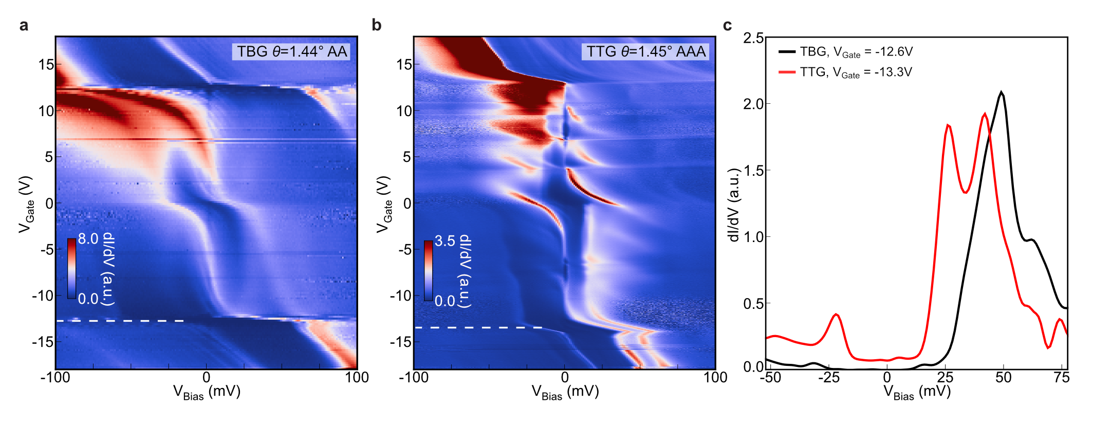
Extended Data Fig. 1: Spectroscopy of twisted bilayer and twisted trilayer graphene. a, Point spectra of twisted bilayer graphene (TBG) on an AA site at a twist angle $\theta=1.44\degree$, from a bilayer region found in the same sample. b, Point spectra of twisted trilayer graphene (TTG) on an AAA site at a twist angle $\theta=1.45\degree$. Unlike TBG at the similar angle, signatures of correlations, such as enhancement of VHS separations at charge neutrality and cascade of flavor symmetry breaking, are observed. c, Linecuts taken from a and b around $\nu=-4$ (white dashed lines). While the $dI/dV\sim\text{LDOS}$ between the flat bands and the remote band is zero for TBG, the value is finite for TTG due to the existence of the additional Dirac cones.

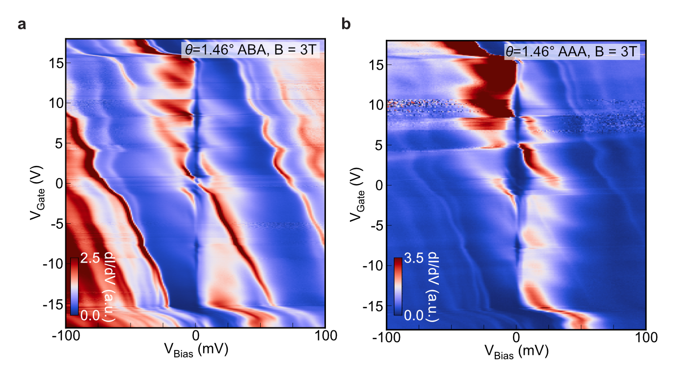
Extended Data Fig. 2: Comparison between spectra on ABA and AAA sites at finite fields. a-b, Point spectroscopy as a function of $V_{\rm Gate}$ on ABA stacked (a, the same as panel Fig. 2d) and on AAA stacked (b) region ($B=3~{}\text{T}$, $\theta=1.46\degree$). In comparison, flat bands appear to be more prominent on the AAA site (b), while LLs from Dirac-like dispersion and dispersive bands appear more pronounced at ABA site. This is a direct consequence of LDOS from the flat bands being localized on the AAA sites. The LDOS from Dirac-like bands is spatially uniformly distributed.

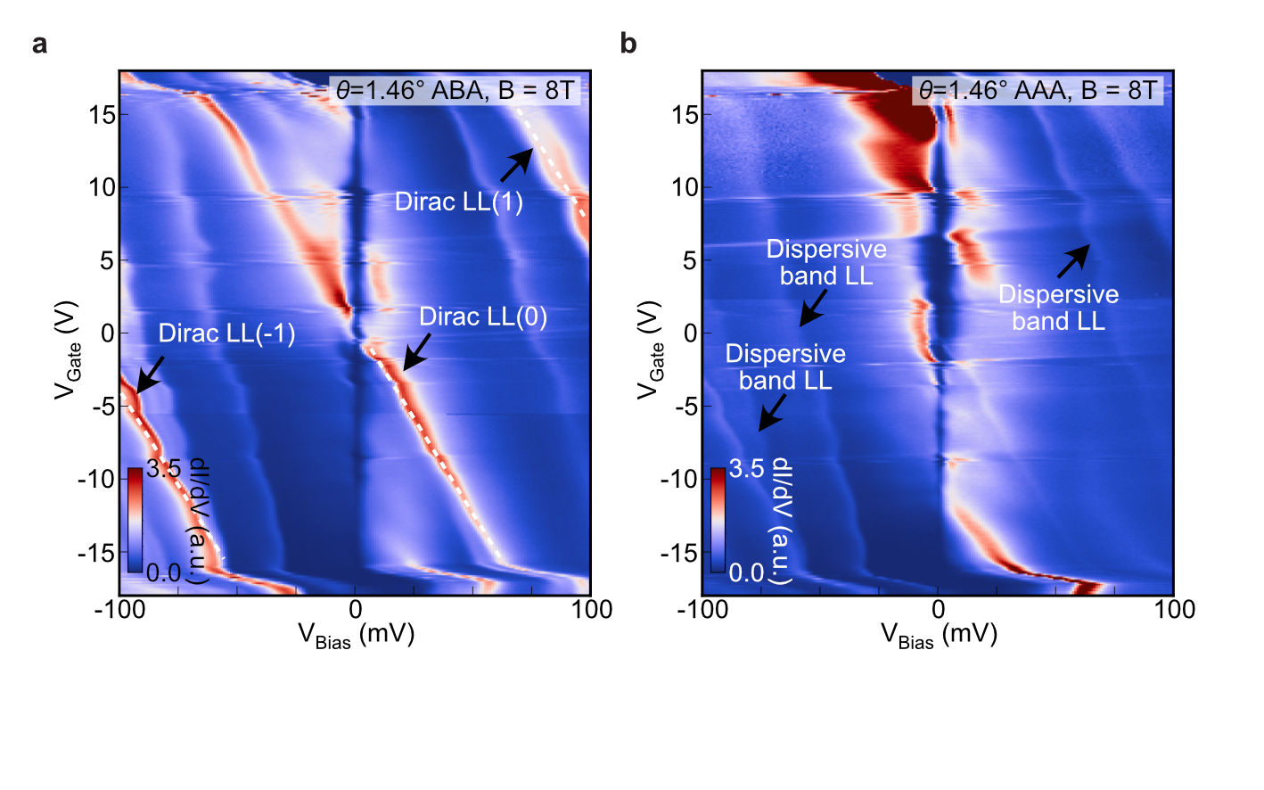
Extended Data Fig. 3: Distinguishing dispersive band LLs and Dirac band LLs a-b, Point spectroscopy as a function of $V_{\rm Gate}$ on ABA stacked (a) and AAA stacked (b) region ($B=8~{}\text{T}$, $\theta=1.46\degree$). Zeroth LL from Dirac dispersion is clearly distinguished from other LLs as it crosses the flat band. Other LLs from Dirac dispersion is distinguished from the dispersive band from being parallel to the zeroth LL as a function of doping. Additional LL is observed at this high magnetic field at $V_{\rm Gate}>12~{}\text{V}$ which is more pronounced at AAA stacked region and can be attributed to second Dirac cone due to finite displacement field present at these $V_{\rm Gate}$.

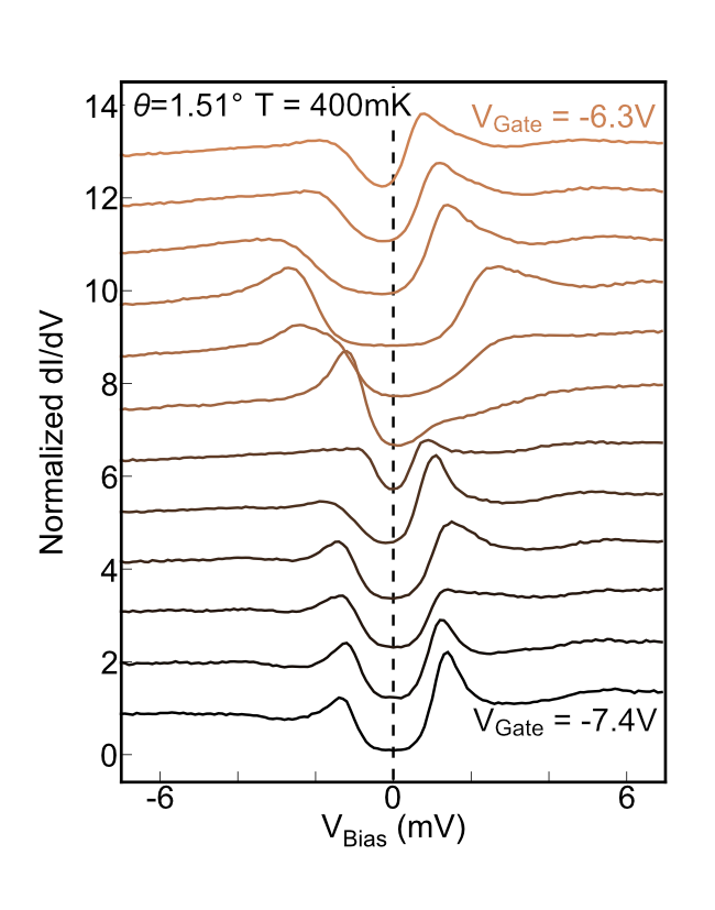
Extended Data Fig. 4: Spectroscopy near $\nu=-2$. Linecuts taken from Fig. 3a for $V_{\rm Gate}$ ranging from $-6.3$ V to $-7.4$ V in $100$ mV steps. Starting from top, the observed gap is highly asymmetric and gradually evolves to the more symmetric spectrum on the bottom. Vertical dashed line shows the position of $V_{\rm Bias}=0~{}\text{mV}$. We interpret that asymmetric gap (brown lines) corresponds to correlated insulator regime, while the symmetric gap (black lines) indicates superconducting regime.

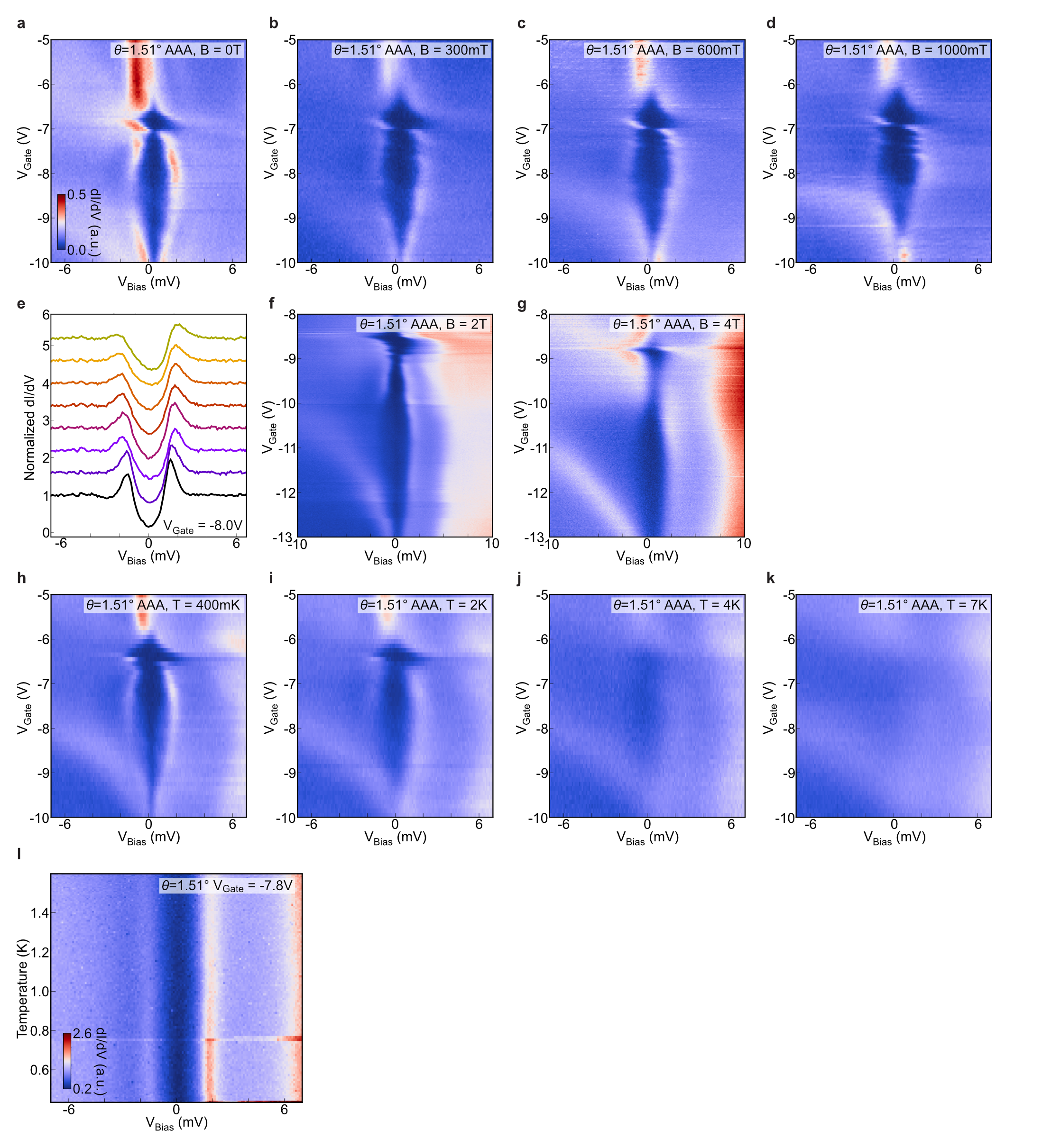
Extended Data Fig. 5: Additional data sets showing magnetic field and temperature dependence of spectroscopic gap in the $\mathbf{-3<\nu<-2}$ range. a-d, Point spectroscopy as a function of $V_{\rm Gate}$ at twist angle of $\mathrm{\theta=1.51\degree}$ at magnetic field $\mathrm{B=0}$ T (a), $\mathrm{B=300}$ mT (b), $\mathrm{B=600}$ mT (c), $\mathrm{B=1}$ T (d). e, Line traces showing magnetic field dependence for $\mathrm{V_{Gate}=-7.8}$ V (U-shaped regime). Color coding corresponds to magnetic field $\mathrm{B=0}$, $0.1$, $0.2$, $0.3$, $0.4$, $0.4$, $0.8$, $1$ T. Plots are offset for clarity. f, g, Gate spectroscopy measured at $B=2$ T (f) and $B=4$ T (g), for $\theta=1.54\degree$ featuring gapped spectrum persisting $B\gtrsim 4$ T (data taken at different point compared to a-e). h-k, Gate spectroscopy taken at different temperatures $\mathrm{T=400}$ mK (h), $\mathrm{T=2}$ K (i), $\mathrm{T=4}$ K (j), $\mathrm{T=7}$ K (k). i, Point spectroscopy measured as a function of $V_{\rm Bias}$ and temperature at the same point as (h-k) for ${V_{\rm Gate}=-7.8}$ V.

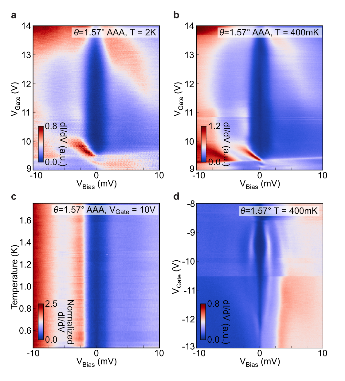
Extended Data Fig. 6: Spectroscopic gap in the $+2<\nu<+3$ range. a, Tunneling conductance spectroscopy at twist angle of $\mathrm{\theta=1.57\degree}$ on AAA stacked region at $\mathrm{T=2}$ K showing well-developed gapped region on the electron-side. b, Spectroscopy measured at the same region at $\mathrm{T=400}$ mK. c, Spectroscopy as a function of temperature at the same point as (a, b) for $\mathrm{V_{Gate}=10V}$. d, Spectroscopy focusing on hole doping taken with the same micro-tip. While the spectrum for hole doping (d) shows clear coherence peaks and dip-hump structures these features are absent for the gap on the electron-side. We speculate that for electron doping, the coherence peaks are suppressed even at our base temperature ($\mathrm{T=400}$ mK). The observed gap in this case is likely originating from pseudogap phase.

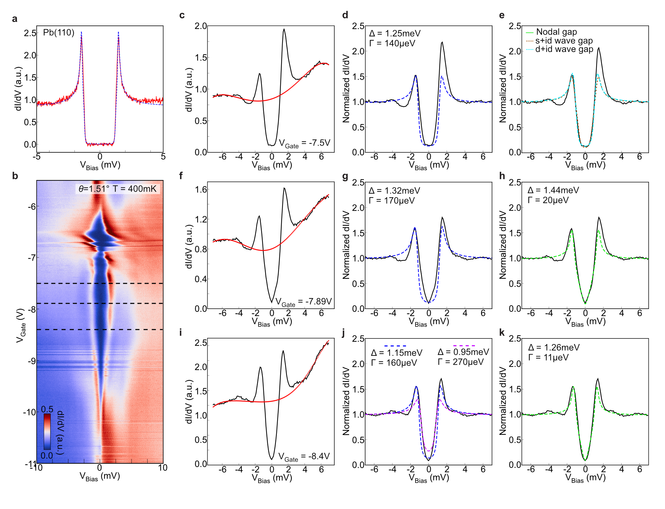
Extended Data Fig. 7: Normalization of tunneling conductance and fitting. a, Tunneling conductance measured on Pb (110) surface at $T=400$ mK showing superconducting gap. Blue dashed line is Dynes formula fit with two gaps with following parameters, $\mathrm{\Delta_{1}=1.42}$ meV, $\mathrm{\Delta_{2}=1.26}$ meV, $\mathrm{\Gamma=10}$ $\mu$eV, $\mathrm{T=400}$ mK used to obtain the base temperature. b, Same data as Fig. 3a showing larger $V_{\rm Bias}$ range. Black dashed lines mark gate voltages $V_{\rm Gate}=-7.5,-7.89,-8.4$ V with the corresponding line traces shown in subsequent panels. c, Line cut in the U-shaped regime ($V_{\rm Gate}=-7.5$ V). Red dotted line is polynomial fitting curve obtained as described in section 5. d, Normalized data obtained by dividing the raw data (black line in c) by polynomial fit (red line in c). Blue line is Dynes formula fit with isotropic gap. e, Same data as d with Dynes formula fits using different types of the pairing gap symmetry: a nodal gap with $\Delta_{d}=1.40$ meV (green); $s+id$ pairing gap with $\Delta_{s}=0.72$ meV, $\Delta_{d}=1.22$ meV (brown); $d+id$ pairing gap with $\mathrm{\Delta_{d1}=1.00}$ meV, $\mathrm{\Delta_{d2}=1.30}$ meV (cyan). f, in the V-shaped regime ($V_{\rm Gate}=-7.89$ V). g, Normalized data from f and Dynes formula fit using an isotropic gap (blue). h, Normalized data from f with Dynes formula fits using a nodal gap with $\Delta=1.44~{}\text{meV}$ (green). i, Another linecut in the V-shaped regime ($V_{\rm Gate}=-8.4~{}\text{V}$). j, Normalized data from i and Dynes formula fit using an isotropic gap (blue, purple). k Normalized data from i and Dynes formula fits green line is nodal gap with $\Delta=1.26~{}\text{meV}$.

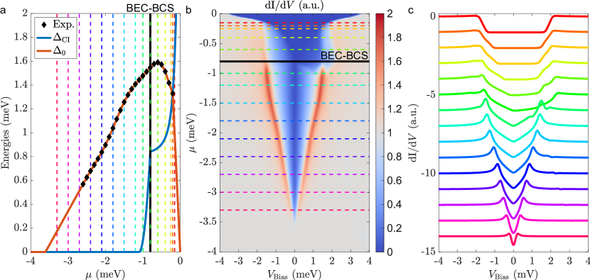
Extended Data Fig. 8: Simulated tunneling conductance across the BEC-BCS transition. a, Chemical potential dependence of $\Delta_{0}$ and $\Delta_{\rm CI}$ used in simulations. Black data points represent coherence-peak locations crudely extracted from experiment, as detailed in the text. b,c, Color map and linecuts of differential conductance $dI/dV$ as a function of $\mu$. Here and in Fig. 3k,j, we set $T=0.05$ meV and employed a nodal $d$-wave gap with $1/2m\ell^{2}=6.25~{}\mu$eV. The BEC-BCS transition manifests as a clear evolution from U- to V-shaped spectra as observed experimentally. We nevertheless stress, as in the text, that panels b,c do not correspond directly to Fig. 3a due in part to the nontrivial relation between chemical potential $\mu$ and filling that has not been incorporated.

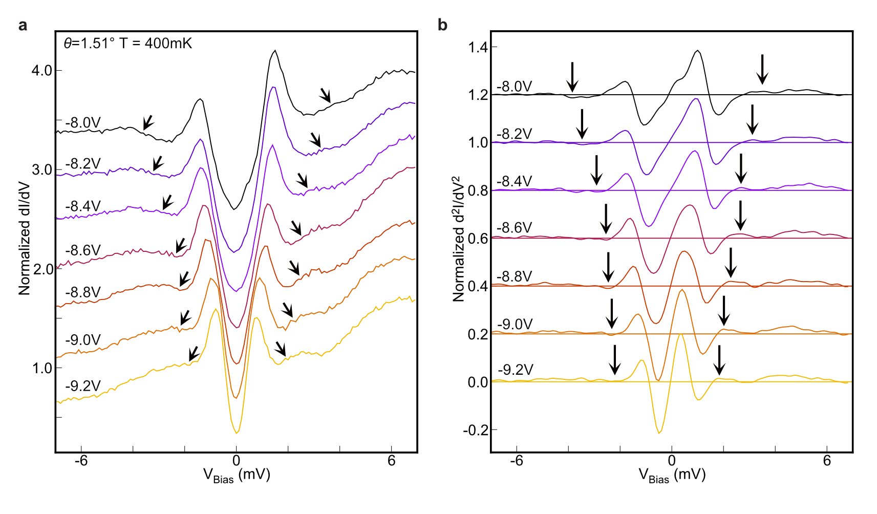
Extended Data Fig. 9: Peak-dip-hump analysis from $d^{2}I/dV^{2}$ local minima/maxima. a, Hole-side superconducting gap spectrum measured at various $V_{\rm Gate}$ ranging from $-8.0~{}\text{V}$ to $-9.2~{}\text{V}$ at $\theta=1.51\degree$ region which is same dataset as Fig. 4a. b, $d^{2}I/dV^{2}$ as a function of $V_{\rm Bias}$ by taking the first derivative of the (a) and apply Gaussian filtering to make the trend clear. The horizontal lines of the same color indicate the $d^{2}I/dV^{2}=0$ for each $V_{\rm Gate}$.

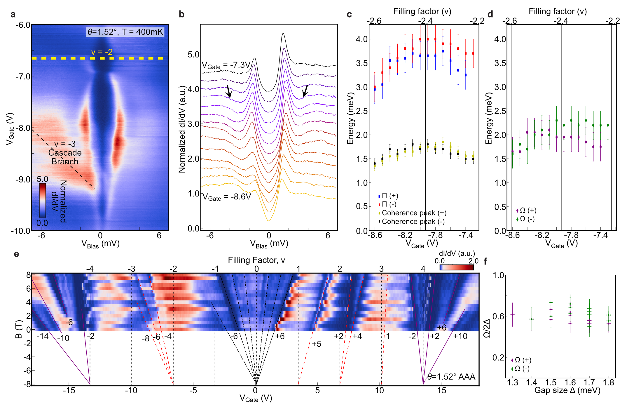
Extended Data Fig. 10: Dip-hump structures observed at different magic-angle area a, Gate spectroscopy measured at $\theta=1.51\degree$. b, Normalized point spectra at range of $V_{\rm Gate}$ from $-8.6~{}\text{V}$ to $-7.3~{}\text{V}$. c, Extracted position of the dip-hump and a coherence peak versus $V_{\rm Gate}$ for $V_{\rm Bias}>0$ (blue and yellow, respectively) and for $V_{\rm Bias}<0$ (red and black, respectively). d, Energy of the bosonic mode versus $V_{\rm Gate}$, obtained by subtracting the corresponding energies of the dip-hump feature and the coherence peak for $V_{\rm Bias}>0$ (purple) and $V_{\rm Bias}<0$ (green). e, LDOS Landau fan diagram measured at the same area as a on AAA region. Black lines indicate the gap between LLs emanating from CNP. Red dashed lines indicate gaps between LLs emanating from integer filling $\nu\neq 0$ of the flat bands. f, $\Omega/2\Delta$ versus $\Delta$ obtained from c,d. In this particular area the dip-hump structure could be resolved mostly in U-shaped regime.

References

- [1] Park, J. M., Cao, Y., Watanabe, K., Taniguchi, T. & Jarillo-Herrero, P. Tunable strongly coupled superconductivity in magic-angle twisted trilayer graphene. Nature 590, 249–255 (2021).
- [2] Hao, Z. et al. Electric field–tunable superconductivity in alternating-twist magic-angle trilayer graphene. Science 371, 1133–1138 (2021).
- [3] Khalaf, E., Kruchkov, A. J., Tarnopolsky, G. & Vishwanath, A. Magic angle hierarchy in twisted graphene multilayers. Phys. Rev. B 100, 085109 (2019).
- [4] Li, X., Wu, F. & MacDonald, A. H. Electronic Structure of Single-Twist Trilayer Graphene. arXiv:1907.12338 [cond-mat] (2019). eprint 1907.12338.
-
[5]
Spectroscopic signatures of nodal pairing and
unconventional superconductivity in magic-angle bilayers were reported in
August 2021 talks by Ali Yazdani’s Group. K. P. Nuckolls,
Thomas Young Centre Moiré-Twistronics Workshop. See also:
Oh, M., Nuckolls, K. P., Wong, D., Lee, R. L., Liu, X., Watanabe, K., Taniguchi, T., Yazdani, Ali, Evidence for unconventional superconductivity in twisted bilayer graphene, arXiv:2109.13944 (2021). - [6] Carr, S. et al. Ultraheavy and Ultrarelativistic Dirac Quasiparticles in Sandwiched Graphenes. Nano Lett. 20, 3030–3038 (2020).
- [7] Kerelsky, A. et al. Maximized electron interactions at the magic angle in twisted bilayer graphene. Nature 572, 95–100 (2019).
- [8] Choi, Y. et al. Electronic correlations in twisted bilayer graphene near the magic angle. Nature Physics 15, 1174–1180 (2019).
- [9] Xie, Y. et al. Spectroscopic signatures of many-body correlations in magic-angle twisted bilayer graphene. Nature 572, 101–105 (2019).
- [10] Jiang, Y. et al. Charge order and broken rotational symmetry in magic-angle twisted bilayer graphene. Nature 573, 91–95 (2019).
- [11] Zondiner, U. et al. Cascade of phase transitions and Dirac revivals in magic-angle graphene. Nature 582, 203–208 (2020). eprint 1912.06150.
- [12] Wong, D. et al. Cascade of electronic transitions in magic-angle twisted bilayer graphene. Nature 582, 198–202 (2020).
- [13] Choi, Y. et al. Correlation-driven topological phases in magic-angle twisted bilayer graphene. Nature 589, 536–541 (2021).
- [14] Fischer, A. et al. Unconventional Superconductivity in Magic-Angle Twisted Trilayer Graphene. arXiv:2104.10176 [cond-mat] (2021). eprint 2104.10176.
- [15] Phong, V. T., Pantaleón, P. A., Cea, T. & Guinea, F. Band Structure and Superconductivity in Twisted Trilayer Graphene. arXiv:2106.15573 [cond-mat] (2021). eprint 2106.15573.
- [16] Choi, Y. et al. Interaction-driven Band Flattening and Correlated Phases in Twisted Bilayer Graphene. arXiv:2102.02209 [cond-mat] (2021). eprint 2102.02209.
- [17] Guinea, F. & Walet, N. R. Electrostatic effects, band distortions, and superconductivity in twisted graphene bilayers. PNAS 115, 13174–13179 (2018).
- [18] Rademaker, L., Abanin, D. A. & Mellado, P. Charge smoothening and band flattening due to Hartree corrections in twisted bilayer graphene. Phys. Rev. B 100, 205114 (2019).
- [19] Goodwin, Z. A. H., Vitale, V., Liang, X., Mostofi, A. A. & Lischner, J. Hartree theory calculations of quasiparticle properties in twisted bilayer graphene. Electron. Struct. 2, 034001 (2020). eprint 2004.14784.
- [20] Calderón, M. J. & Bascones, E. Interactions in the 8-orbital model for twisted bilayer graphene. Phys. Rev. B 102, 155149 (2020). eprint 2007.16051.
- [21] Christos, M., Sachdev, S. & Scheurer, M. S. Correlated insulators, semimetals, and superconductivity in twisted trilayer graphene. arXiv:2106.02063 [cond-mat] (2021). eprint 2106.02063.
- [22] Jung, S. et al. Evolution of microscopic localization in graphene in a magnetic field from scattering resonances to quantum dots. Nature Physics 7, 245–251 (2011).
- [23] Eagles, D. M. Possible Pairing without Superconductivity at Low Carrier Concentrations in Bulk and Thin-Film Superconducting Semiconductors. Phys. Rev. 186, 456–463 (1969).
- [24] Renner, C., Revaz, B., Genoud, J.-Y., Kadowaki, K. & Fischer, Ø. Pseudogap Precursor of the Superconducting Gap in Under- and Overdoped Bi2Sr2CaCu2O8+. Phys. Rev. Lett. 80, 149–152 (1998).
- [25] Rodan-Legrain, D. et al. Highly tunable junctions and non-local Josephson effect in magic-angle graphene tunnelling devices. Nat. Nanotechnol. 16, 769–775 (2021).
- [26] Dynes, R. C., Narayanamurti, V. & Garno, J. P. Direct Measurement of Quasiparticle-Lifetime Broadening in a Strong-Coupled Superconductor. Phys. Rev. Lett. 41, 1509–1512 (1978).
- [27] Yeh, N.-C. et al. Evidence of Doping-Dependent Pairing Symmetry in Cuprate Superconductors. Phys. Rev. Lett. 87, 087003 (2001).
- [28] Botelho, S. S. & Sá de Melo, C. A. R. Lifshitz transition in $d$-wave superconductors. Phys. Rev. B 71, 134507 (2005).
- [29] Borkowski, L. & de Melo, C. S. Evolution from the BCS to the Bose-Einstein Limit in a d-Wave Superconductor at T=0. Acta Physica Polonica A 6, 691–698 (2001).
- [30] Chen, Q., Stajic, J., Tan, S. & Levin, K. BCS–BEC crossover: From high temperature superconductors to ultracold superfluids. Physics Reports 412, 1–88 (2005).
- [31] Randeria, M. & Taylor, E. Crossover from Bardeen-Cooper-Schrieffer to Bose-Einstein Condensation and the Unitary Fermi Gas. Annual Review of Condensed Matter Physics 5, 209–232 (2014).
- [32] Schrieffer, J. R., Scalapino, D. J. & Wilkins, J. W. Effective Tunneling Density of States in Superconductors. Phys. Rev. Lett. 10, 336–339 (1963).
- [33] McMillan, W. L. & Rowell, J. M. Lead Phonon Spectrum Calculated from Superconducting Density of States. Phys. Rev. Lett. 14, 108–112 (1965).
- [34] Lee, J. et al. Interplay of electron–lattice interactions and superconductivity in Bi2Sr2CaCu2O8+. Nature 442, 546–550 (2006).
- [35] Niestemski, F. C. et al. A distinct bosonic mode in an electron-doped high-transition-temperature superconductor. Nature 450, 1058–1061 (2007).
- [36] Chi, S. et al. Scanning Tunneling Spectroscopy of Superconducting LiFeAs Single Crystals: Evidence for Two Nodeless Energy Gaps and Coupling to a Bosonic Mode. Phys. Rev. Lett. 109, 087002 (2012).
- [37] Shan, L. et al. Evidence of a Spin Resonance Mode in the Iron-Based Superconductor Ba0.6K0.4Fe2As2 from Scanning Tunneling Spectroscopy. Phys. Rev. Lett. 108, 227002 (2012).
- [38] Zasadzinski, J. F. et al. Correlation of Tunneling Spectra in Bi2Sr2CaCu2O8+ with the Resonance Spin Excitation. Phys. Rev. Lett. 87, 067005 (2001).
- [39] Ramires, A. & Lado, J. L. Emulating Heavy Fermions in Twisted Trilayer Graphene. Phys. Rev. Lett. 127, 026401 (2021).
- [40] Carbotte, J. P. Properties of boson-exchange superconductors. Rev. Mod. Phys. 62, 1027–1157 (1990).
- [41] Song, C.-L. & Hoffman, J. E. Pairing insights in iron-based superconductors from scanning tunneling microscopy. Current Opinion in Solid State and Materials Science 17, 39–48 (2013).
- [42] Scalapino, D. J., Schrieffer, J. R. & Wilkins, J. W. Strong-Coupling Superconductivity. I. Phys. Rev. 148, 263–279 (1966).
- [43] Yu, G., Li, Y., Motoyama, E. M. & Greven, M. A universal relationship between magnetic resonance and superconducting gap in unconventional superconductors. Nature Phys 5, 873–875 (2009).
- [44] Anderson, P. W. & Ong, N. P. Theory of asymmetric tunneling in the cuprate superconductors. Journal of Physics and Chemistry of Solids 67, 1–5 (2006).
- [45] Eschrig, M. & Norman, M. R. Effect of the magnetic resonance on the electronic spectra of high-Tc superconductors. Phys. Rev. B 67, 144503 (2003).
- [46] Khalaf, E., Chatterjee, S., Bultinck, N., Zaletel, M. P. & Vishwanath, A. Charged skyrmions and topological origin of superconductivity in magic-angle graphene. Science Advances 7, eabf5299 (2021). eprint 2004.00638.
- [47] Choi, Y. W. & Choi, H. J. Dichotomy of Electron-Phonon Coupling in Graphene Moire Flat Bands. arXiv:2103.16132 [cond-mat] (2021). eprint 2103.16132.
- [48] Reznik, D. et al. Electron–phonon coupling reflecting dynamic charge inhomogeneity in copper oxide superconductors. Nature 440, 1170–1173 (2006).
- [49] Le Tacon, M. et al. Inelastic X-ray scattering in YBa2Cu3O6.6 reveals giant phonon anomalies and elastic central peak due to charge-density-wave formation. Nature Phys 10, 52–58 (2014).
- [50] Gabovich, A. M. & Voitenko, A. I. Charge density waves as the origin of dip-hump structures in the differential tunneling conductance of cuprates: The case of d-wave superconductivity. Physica C: Superconductivity and its Applications 503, 7–13 (2014).
- [51] Cao, Y. et al. Nematicity and competing orders in superconducting magic-angle graphene. Science 372, 264–271 (2021).
- [52] Lewandowski, C., Chowdhury, D. & Ruhman, J. Pairing in magic-angle twisted bilayer graphene: Role of phonon and plasmon umklapp. Phys. Rev. B 103, 235401 (2021).
- [53] Chou, Y.-Z., Wu, F., Sau, J. D. & Sarma, S. D. Correlation-induced triplet pairing superconductivity in graphene-based moir\’e systems. arXiv:2105.00561 [cond-mat] (2021). eprint 2105.00561.
- [54] Bistritzer, R. & MacDonald, A. H. Moiré bands in twisted double-layer graphene. PNAS 108, 12233–12237 (2011).
- [55] Cea, T., Walet, N. R. & Guinea, F. Electronic band structure and pinning of Fermi energy to Van Hove singularities in twisted bilayer graphene: A self-consistent approach. Phys. Rev. B 100, 205113 (2019).
- [56] Zasadzinski, J. F., Coffey, L., Romano, P. & Yusof, Z. Tunneling spectroscopy of Bi2Sr2CaCu2O8+ Eliashberg analysis of the spectral dip feature. Phys. Rev. B 68, 180504 (2003).
- [57] Pistolesi, F. & Strinati, G. C. Evolution from BCS superconductivity to Bose condensation: Calculation of the zero-temperature phase coherence length. Phys. Rev. B 53, 15168–15192 (1996).
- [58] Stintzing, S. & Zwerger, W. Ginzburg-Landau theory of superconductors with short coherence length. Phys. Rev. B 56, 9004–9014 (1997).
- [59] Cao, G., He, L. & Zhuang, P. BCS-BEC quantum phase transition and collective excitations in two-dimensional Fermi gases with $p$- and $d$-wave pairings. Phys. Rev. A 87, 013613 (2013).