Intracluster Light Properties in a Fossil Cluster at z=0.47

Abstract

Galaxy clusters contain a diffuse stellar component outside the cluster’s galaxies, which is observed as faint intracluster light (ICL). Using Gemini/GMOS-N deep imaging and multi-object spectroscopy of a massive fossil cluster at a redshift of $z=0.47$, RX J105453.3+552102 (J1054), we improve the observational constraints on the formation mechanism of the ICL. We extract the ICL surface brightness and colour profiles out to 155 kpc from the brightest cluster galaxy (BCG) with a detection limit of 28.7 mag/arcsec² (1$\sigma$, $4.8\arcsec\times 4.8\arcsec$; i–band). The colour of the diffuse light is similar to that of the BCG and central bright galaxies out to $\sim$ 70 kpc, becoming slightly bluer toward the outside. We find that the ICL distribution shows better agreement with the spatial distribution of member galaxies than with the BCG-dominated cluster luminosity distribution. We report the ICL fraction of J1054 as $15.07\pm 4.57\%$ in the range of $60\sim 155$ kpc from the BCG, which appears to be higher than the ICL fraction-redshift trend in previous studies. Our findings suggest that intracluster stars seems not to be explained by one dominant production mechanism. However, a significant fraction of the ICL of J1054 may have been generated from the outskirts of infalling/satellite galaxies more recently rather than by the BCG at the early stage of the cluster.

1 Introduction

Recent deep observations of nearby galaxy clusters show distinct diffuse intracluster light (ICL), referring to the light from stars that are not bound to any individual cluster galaxy (Zwicky, 1951; Gregg & West, 1998; Feldmeier et al., 2002; Lin & Mohr, 2004; Gonzalez et al., 2005; Zibetti et al., 2005; Mihos et al., 2005; Mihos et al., 2017; DeMaio et al., 2018; Jiménez-Teja et al., 2019; Kluge et al., 2020; Furnell et al., 2021; Montes et al., 2021). The ICL is expected to follow the global potential well of the galaxy cluster and can therefore be used as a luminous tracer for dark matter (Montes & Trujillo, 2018, 2019; Alonso Asensio et al., 2020). Furthermore, accounting for the ICL could bolster our understanding of the baryon component of the universe (Buote et al., 2016) and reduce the discrepancy between observations and cosmological simulations. In other words, observations of the distribution and abundance of ICL would impose a strong constraint on theoretical models of the evolution of galaxy clusters (Lin & Mohr, 2004; Arnaboldi & Gerhard, 2010).

The abundance of ICL increases through numerous galaxy interactions in galaxy clusters, as suggested by simulation studies (Murante et al., 2007; Purcell et al., 2007; Conroy et al., 2007; Puchwein et al., 2010; Rudick et al., 2011; Contini et al., 2014; Cooper et al., 2015). Observations also reported several scenarios for the production of intracluster stars, including brightest cluster galaxies (BCG) major mergers and violent relaxation afterwards (Rines et al., 2007; Ko & Jee, 2018), tidal stripping from the outskirts of L^∗ member galaxies (Iodice et al., 2017; DeMaio et al., 2018; Montes & Trujillo, 2018), disruptions of dwarf galaxies as they fall towards galaxy cluster centres (Toledo et al., 2011) and in-situ star formation (Gerhard et al., 2002). However, the main ICL formation mechanism is still under debate due to a lack of ICL measurements over a wide range of redshifts and masses with an equal observational method of measuring the ICL properties.

Within this paradigm, whereby a significant fraction of intracluster stars has been stripped from cluster galaxies through multiple mechanisms, we can expect that the amount of ICL (the ICL fraction; diffuse light to cluster total light fraction) can act as a measurement tool for estimating the dynamic states of galaxy clusters (Mihos, 2016; Montes, 2019). For example, more evolved clusters should have a higher ICL fraction compared to dynamic young clusters. Values in previous studies of ICL fractions vary immensely, from 2.6% (McGee & Balogh, 2010) to 50% (Lin & Mohr, 2004), largely because the observed ICL fraction varies according to the cluster’s dynamical state. In this context, important constraints thus come from ICL measurements in the most evolved (dynamically relaxed) galaxy clusters.

According to the current Lambda cold dark matter ($\Lambda$CDM) model, virialised halos grow by hierarchical merging. Fossil clusters (Ponman et al., 1994; Jones et al., 2003; Cypriano et al., 2006) are galaxy clusters in which the accretion rate is fast and efficient, resulting in luminosity-dominant BCGs (D’Onghia et al., 2005). Fossil clusters are defined as having an absolute magnitude gap in the r–band between the BCG and the second brightest galaxy ($\Delta M_{12}$) that exceeds 2, containing extended X-ray sources with $L_{X}>10^{42}erg/s$ (Jones et al., 2003). In fossil clusters, all significant merging and violent relaxation events have already taken place, thus we regard them as dynamically evolved and relaxed systems. Because they may have undergone significant dynamic processes which enrich both the ICL and the BCG (Contini et al., 2014; Contini et al., 2019), fossil clusters are expected to have the most abundant ICL fraction among galaxy clusters with similar redshifts and masses. Moreover, the dominant BCGs of fossil clusters allow us to assume a common assembly history, which is “hierarchical merging toward one central mass."

Measuring the ICL fraction in fossil clusters at various redshifts will thus help us improve our understanding about ICL formation and evolution. However, high-z samples are very limited, as fossil clusters are themselves rare (Jones et al., 2003; Tavasoli et al., 2011) and there is too little spectroscopic membership data to fulfil the definition of a fossil cluster. The detection of ICL in high-z fossil clusters is even more challenging due to its faintness. Although several intermediate-z fossil clusters have been discovered (Ulmer et al., 2005; Pierini et al., 2011), ICL has not been studied in detail in relation to fossil clusters. The only fossil cluster for which there has been an ICL study is Abell 2261 at a redshift of $\sim$ 0.22 with an ICL fraction $\sim$ 16.64% (Burke et al., 2015).

There is a consensus that most intracluster stars are produced after $z\sim 1$ (e.g., Puchwein et al., 2010; Rudick et al., 2011; Cooper et al., 2015). Interestingly, some studies (Contini et al., 2014; Burke et al., 2015; Lin et al., 2017) claim that the majority of the stellar mass of BCGs has assembled by $z\sim 0.4$ and that the accreted stellar mass after this epoch mainly contributes to the growth of the present-day ICL. If BCG growth is the main ICL formation mechanism, then the ICL fraction at $z\sim 0.4-0.5$ is likely to be as high as that of local galaxy clusters and the colour of the ICL is likely to be similar to that of the BCG (optically red). If tidal stripping/disruption of infalling/satellite galaxies is the main mechanism, the ICL fraction is likely to show a strong evolution from $z\sim 0.4-0.5$, and its colour would be much bluer than BCG and galaxies near the cluster core because stripped stars mainly originate from the outskirts of galaxies with low metallicity or blue dwarf galaxies with young stellar populations. Thus, fossil clusters around $z\sim 0.4-0.5$ can be an optimal target to examine the BCG-related ICL formation scenario.

Here, we report measurements of the ICL distribution, colour, and fraction relative to the total cluster light using deep optical imaging and multi-object spectroscopy data of a fossil cluster at $z=0.47$. To date, this is the most distant fossil cluster for which the distribution and abundance of ICL have been measured.

This paper has the following structure. We describe the details of our observations and the data reduction procedure in Section 2. We analyse the robustness of the ICL measurement scheme in Section 3. In Section 4, we report the results of the ICL measurements and galaxy cluster properties. The possible ICL formation scenario based on the results is discussed in Section 5. Finally, we summarise and conclude the paper in Section 6. Throughout the paper, we adopt a standard $\Lambda$CDM model with $H_{0}$=70 km s^-1 Mpc^-1, $\Omega_{m}$=0.3 and $\Omega_{\Lambda}$=0.7, providing an angular scale of 5.89 kpc arcsec^-1 at a redshift of the target cluster. Magnitudes are expressed in the AB magnitude system.

2 Data

We conducted deep imaging observations and multi-object spectroscopy (MOS) of the fossil cluster at $z=0.47$ using the GMOS-N instrument (Hook et al., 2004) of the 8.1 meter Gemini North telescope. The field of view of GMOS is $5.5^{\prime}\times 5.5^{\prime}$, which corresponds to $\sim$ 2.0 Mpc $\times$ 2.0 Mpc at the redshift of the target cluster. The data were obtained in April and May of 2018 (GN-2018A-Q-201/PI: Jaewon Yoo). Table 2 describes our observations, including the date, seeing conditions, filters, the number of exposures, and the exposure time per visit. Using the Gemini IRAF package, we performed basic data reduction following the Gemini data reduction cookbook (Shaw, 2016).

2.1 Target cluster selection

We selected our target galaxy cluster from the fossil system candidates (Santos et al., 2007), which are based on the SDSS DR5 (Adelman-McCarthy et al., 2007) and ROSAT (Voges et al., 1999) catalogues. Among the 34 fossil system candidates in Santos et al., we initially selected massive galaxy clusters using an X-ray luminosity cut, i.e. $L_{X}\geq 10^{44}erg/s$. In the SDSS DR14 (Abolfathi et al., 2018) catalogue, we retrieved potential member galaxies (within a projected radius of 500 kpc from the BCG and with a photometric redshift cut $z_{BCG}\pm 0.05$) of the galaxy clusters. The photometric redshift is based on the kd-tree nearest neighbor fit method (Csabai et al., 2007). In the redshift range of $0.4<z<0.5$, we selected RX J105453.3+552102 (hereafter J1054), which is one of the fossil group origins (FOGO) project samples that has been confirmed as a fossil cluster with $\Delta M_{12}=2.12\pm 0.33$ (Aguerri et al., 2011; Zarattini et al., 2014). Table 1 lists the key properties of J1054.

The presence of the galactic cirrus can lead to misinterpretations in ICL measurements. For this reason, we checked the Planck 2015 dust map (Planck Collaboration et al., 2016). The target cluster field has no extended emission. Additionally, we found E(B–V)=$0.0088\pm 0.0003$ for the target field from another dust map (based on Gaia, Pan-STARRS 1, and 2MASS) provided by Green et al. (2019).

Table 1: Target description

SDSS name	ROSAT name	R.A	Dec	z	$L_{X}$	$r_{200}^{a}$	$M_{200}^{a}$
		(h:m:s)	(d:m:s)		[$10^{44}erg/s$]	[Mpc]	[$10^{14}M_{\odot}$]
J105452.03+552112.5	RX J105453.3+552102	10:54:52.03	+55:21:12.5	0.47	2.39	1.68	5.40
a The $r_{200}$ and the $M_{200}$ are calculated in Section 4.2.2.

2.2 Observations and reductions

Table 2: GMOS-N observation

Observation Date	Days from	Seeingb	Moffat $\beta$b	Filter	Number of exposure	Exposure time per visit	Used in science
(YYYY-mm-dd)	New Moon	[arcsec]				[s]
2018-04-11	25	0.97″	2.65	i	24	178	Yes
2018-05-19	4	-	-	r	6	170	No
2018-05-21	6	-	-	i	4	178	No
2018-05-21	6	0.76″	3.06	r	19	170	Yes
2018-05-21	6	-	-	OG515 (MOS)	3	600	Yes
b Point spread function (PSF) of each band image is modeled using the PSFex (Bertin, 2011) routine.

Measurements of the ICL demand careful observations and data reduction (Mihos et al., 2005; Duc et al., 2015; Capaccioli et al., 2015; Trujillo & Fliri, 2016; Borlaff et al., 2019; Román et al., 2020; Montes et al., 2021). In general, the key during ICL measurements is to minimise the level of sky background error, mostly dominated by residual flat-fielding inaccuracies on a large scale and sky background subtraction. We describe below the observational strategy and data processing method in detail to achieve our goal in this study.

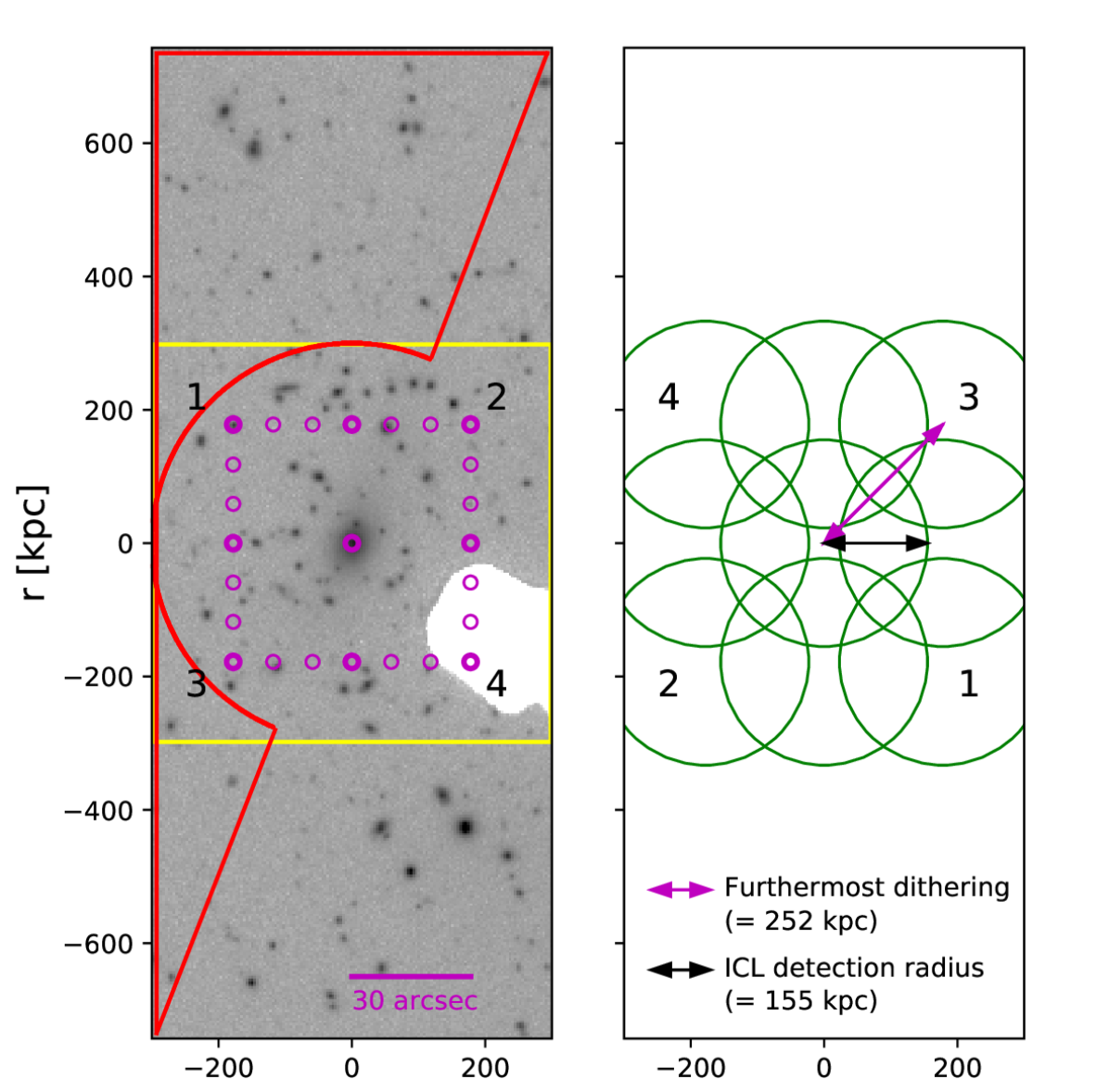
Figure 1: (Left) The i–band deep image of the J1054 cluster. Here, 24 exposure frames are combined and the corresponding full exposure area is shown. The scales are inverse and log-scaled. The dithering patterns are denoted by the magenta circles. The furthermost dither is $42.5^{\prime\prime}$ ($\sim$ 252 kpc) away from the centre. The white region toward the south is where the guide arm is located. The background level and corresponding error are measured in the red defined region. (Right) Animation of the dithering strategy. From the nine dithering points (indicated by the thick magenta circles in the panel on the left), predicted ICL regions in the sky flat are indicated by the green circles. The numbers 1 - 4 indicate the ICL region corresponding to the dithering position with the same numbering in the left panel. See the text for more details about the observation strategy and the masking done for the analysis.

Observation strategy: In the field of the cluster, there is a bright foreground star (cModelMag $m_{i}$=14.58 mag) which imposes a strong limit on the exposure time. To reach a low surface brightness regime, we decided to use this as a guide star to be covered by a guiding arm, thus securing an appropriate exposure time and reducing overhead. We took dithering steps large (furthermost dithering from the centre is 42.5″; see Figure 1) enough to prevent the central region of the cluster from being overlapped between exposures and to obtain a flat background around the cluster ICL region. This also allows us to make sky flats, removing the area vignetted by the guiding arm.

To measure the colour of the ICL and cluster member galaxies, we decided to observe in two bands, the passband i– and r–bands, as they allow, detection of the red sequence using the 4000Å break and have good instrument sensitivity. After blocking the brightest star, to prevent saturation by other bright stars from affecting the ICL analysis, the single exposure time was designed to be 178s and 170s for the i–band and r–band, respectively. The observed exposure time is 83 minutes for the i–band and 71 minutes for the r–band (see Table 2). The original field of view of GMOS is $5.5^{\prime}\times 5.5^{\prime}$; nonetheless, we decided to use only part of the image given that our analysis is extremely sensitive to background noise. After dithering and avoiding chip gaps, the final image area covered by every exposure has a size of $1.7^{\prime}\times 4.0^{\prime}$. This area of full exposure corresponds to 600 kpc $\times$ 1415 kpc at the target redshift with a radius of 300 kpc from the BCG centre.

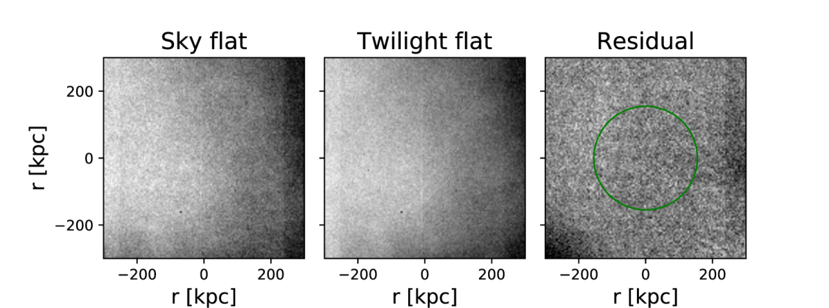
Figure 2: (Left) The i–band sky flat generated by combining 24 science images. The central 600 kpc $\times$ 600 kpc region (indicated by the yellow box in Figure 1) of the cluster, where we measure the ICL, is plotted. (Middle) For the same region, the i–band twilight flat generated by combining 34 twilight images. (Right) The residual (sky flat – twilight flat) image. Its standard deviation is 0.003. The green circle indicates the central region with a radius of 155 kpc, within which the ICL analysis is conducted. The scales are z-scaled and the scale bar of each image is plotted on the bottom side. The residual image shows that the sky flat does not have artefacts from bright objects or from the guide arm (see the panel on the left in Figure 1 for their location).

Flat-fielding: Flat-fielding is a crucial step in the data reduction process for low surface-brightness science. To minimise inaccuracies during flat-fielding, we created sky flats using our science images taken on the same night (i.e., 24 and 19 images taken during one night for the i– and r–bands, respectively). For each science image, we masked out objects (more than 3$\sigma$ from the median) over two iterations and normalised each image using the mode value. The masked and scaled input images were then median-combined to form a single sky flat.

The large offsets between exposures (for each exposure, 19 exposures are at least 178 kpc away) allow the central region near the BCG, where we measure the ICL and cluster galaxies to prevent them as much as possible from occupying the same physical region of the detector in all science exposures. In Figure 2, we show the difference between the sky and twilight flats in the i–band. The standard deviation of the residual image is 0.003. Within the central region where we measure the ICL (the green circle in Figure 2), our sky flat does not show any trend of higher pixel values compared to the twilight flat, which is free from central diffuse light and the guiding arm. Thus, our sky flat is not affected by any gradient caused by diffuse light in the cluster central region. Moreover, artifacts from the guide arms are naturally removed when the images are stacked. The absence of any suspicious residual light possibly affected by the guide arm furthermore ensured us that the effect of the guide arm on our sky flat is negligible.

Astrometry refinement: For the refinement of the astrometry of all of our science images, we used the mscfinder.msctpeak task in IRAF, as suggested in the Gemini data reduction cookbook. This task allowed us to characterise the distortions through the TNX projection, which is an experimental tangent plane projection method. We take as a reference the astrometry of the stars in the SDSS DR14 catalogue. To do this, we selected SDSS stars across the image, satisfying our point source criteria, psfMag_i-cModelMag_i $<0.2$ and non-saturated 20 $<$ cModelMag_i $<$ 22. The cModelMag value is derived from a linear combination of the exponential fit and the de Vaucouleurs fit, and a perfect point source would have an exponentially decaying radial profile. Therefore, the cModelMag and point spread function fitted psfMag values have excellent agreement for stars (Abazajian et al., 2004). Through these criteria, 50 stars were selected and approximately 40 stars were matched in each image. We found that the astrometry precision is about $0.02\arcsec$.

Sky subtraction: Another critical step is consistent sky subtraction for all science exposures before image stacking. We determine the global sky level for each exposure by estimating the median of the statistical distribution of pixels in the image with sigma-clipping over five iterations using the imstatistics task in IRAF and subtract this value from the individual images. If the ICL is non-negligible on a large scale (in the central region near the BCG), the sky level is likely to be overestimated and the ICL will therefore be underestimated. However, we do not have to worry about this removal of the ICL because we later separately measure the sky background level again from the final stacked image. Above this background level, the ICL is quantified by measuring the excess surface brightness.

Image coaddition: Final stacking of the individual science images was performed using the imcoadd task in IRAF. After removing artefacts (bad pixels, cosmic rays, satellite tracks) individual images were median-combined. The image resampling method used here is nearest. Figure 1 shows the full exposure area in the i–band.

PSF matching: The reduced i–band images were taken in slightly worse seeing conditions than the in r–band (see Table 2). Even if we use a common mask for the i– and r–bands (presented in Section 3.2), different PSF profiles could cause the ICL measurements to differ (Trujillo & Fliri, 2016; Karabal et al., 2017). To address this issue, it is necessary to degrade the r–band images (good seeing; 0.76$\arcsec$) down to the seeing level of the i–band images (bad seeing; 0.97$\arcsec$). First, we used PSFex to model the PSFs in the stacked images for the i– and r–band. PSFex gives us a fitted Moffat profile parameter $\beta$ and the full-width half maximum (FWHM), which determine the shape and scale of the PSF profile. Here, we adopt the Moffat PSF profile because it allows a thicker tail compared to the Gaussian option (Trujillo et al., 2001). Then, we convolved the r–band images using the Moffat2DKernel astropy package (Astropy Collaboration et al., 2013) so as to match the PSF of the i–band.

Photometric calibration: Photometric calibration of the images is based on SDSS DR15 (Aguado et al., 2019), comparing the reference magnitude from the SDSS DR15 photometric catalogue to our own. Due to the lack of bright stars (14.5 $<$ psfMag $<$ 19.5; Chonis & Gaskell, 2008), we calculated a weighted mean of 12 stars within our field of view, assigning more weight to brighter stars. The estimated zero-point values are 33.96 mag and 33.93 mag for the i– and r–band, respectively.

2.3 Spectroscopic data

The aim of the MOS observation is to determine the redshifts of potential member galaxies and to confirm cluster members. Galaxy cluster membership is necessary, not only to confirm the target cluster as a fossil cluster, but also to estimate the total cluster light. Although the 78 spectroscopically confirmed member galaxies were already available in the literature (Aguerri et al., 2011), we conducted additional MOS observations to identify more member galaxies. We assigned a slit to the BCG to obtain more detailed spectral information, 16 slits for potential member galaxies, five slits to obtain a sky spectrum and one slit for a standard star to calibrate the fluxes. In the results section, we re-selected cluster member galaxies, including new candidate galaxies from the MOS observation.

The potential member galaxies to assign in MOS slits were selected in a manner similar to that described in Section 2.1. In the SDSS DR14 catalogue, we retrieved galaxies within the GMOS field of view and applied a photometric redshift cut of $z_{BCG}\pm 0.05$. Then, we excluded galaxies that already have spectroscopic data. Among the remaining 28 galaxies, considering the spatial locations of the slits on the mask and prioritising bright and red galaxies, 16 galaxies were assigned via the Gemini MOS Mask Preparation Software (GMMPS) tool.

We used 1″ slit widths and 5″ slit lengths, with the R150 grating and OG515 blocking filter. In each frame two pixels are binned in both the spectral (0.193 nm/pixel) and spatial dimensions. Spectra were obtained by combining dithers at the three central wavelengths of 717, 737, and 757 nm to fill the gaps between the detectors. Three exposures of 600 seconds for each wavelength dithering made the total integration time 30 minutes.

We reduced the MOS data following the official Gemini data reduction cookbook and measured the redshift using SpecPro (Masters & Capak, 2011) in IDL. Among the 16 galaxies in the MOS slits, we could reliably measure the redshifts of three galaxies, whose redshifts estimated to be similar to the BCG redshift. These were therefore included in the cluster member candidates.

3 Analysis

First, we model the stars in Section 3.1. In Sections 3.2 and 3.3, we robustly mask out all luminous objects and determine our background level and the corresponding error for the ICL measurements. We use only the regions where full exposures cover the stacked image. Additionally, we do not use the regions of images where the background value could be contaminated by the glow from the guide arm and/or a bright star with $m_{i}$=17.20 mag.

3.1 Modelling stars

Stars have extended stellar wings which could contaminate the colour of the ICL and its fraction (Uson et al., 1991) and for this reason we mask them out completely. We use the PSFex result (presented in the PSF matching part in Section 2.2) to measure the radius of each extended stellar wing. The Moffat profile,

$$I(r)=I_{0}\left[1+\left(\frac{r}{\alpha}\right)^{2}\right]^{-\beta},$$ (1)

with a scale factor $\alpha=FWHM/2\sqrt{2^{1/\beta}-1}$, is more suitable for describing an extended stellar wing with a thicker tail compared to the Gaussian profile. The resultant Moffat parameter $\beta$ is 2.97 (3.01), and the FWHM is $0.97^{\prime\prime}$ ($0.76^{\prime\prime}$) for the i–band (r–band) image. From the Moffat parameter and the FWHM of each band image, and after substituting the peak ADU value of each star for $I_{0}$ and the background value for $I(r)$, we could calculate the radius of the extended stellar wing of each star analytically.

3.2 Object detection and masking

Object detection is performed using the software SExtractor (Bertin & Arnouts, 1996). For rigorous masking, we choose the code parameters through a visual inspection as DETECT_THRESH 1 $\sigma$, DETECT_MINAREA 3 pixel, BASK_SIZE 64 pixel (corresponding to 60.82 kpc at target redshift), DEBLEND_NTHRESH 1 (minimum deblending to detect bright sources strictly and mask out) and FILTER_NAME gauss_4.0_7x7.conv (matching to the seeing on the observation date). This parameter set is in line with that adopted by Ko & Jee (2018). Considering the ‘cold + hot’ extraction technique (Rix et al., 2004; Barden et al., 2012; Galametz et al., 2013) to detect both extended bright objects and small faint objects, we confirm that our mask (defined by our parameter combination) covers regions of various detection modes in our analysis region.

Our bright source detection method is so rigorous that every stellar wing was within the masked region. We also confirm that all stellar wings are outside our ICL analysis region, which is between 60 kpc and 155 kpc from the centre of the BCG. Masking of both bright objects and extended stellar wings is done in the i–band and applied to both the i– and r–band, as i–band images have larger seeing values and were observed to be deeper than those of the r–band with longer exposure times.

The bright star and guide arm on the south-west side of image in Figure 1 cause a glow that affects the analysis of diffuse light. After checking the affected area using the corresponding radial profiles, we decided to use only the north-east half of the image for the analysis of the ICL (see the top panel in Figure 4). The extended stellar wing of the brightest star measured through the Moffat profile used for guide star has a radius of $7.61^{\prime\prime}$. This value is well within the mask, where the distance from the star to the analysis region is $35.72^{\prime\prime}$.

The reliability of the masking procedure is tested as follows. We draw a radial profile from the centre of the BCG and check the location where it becomes flat, which is 170 kpc from the centre. More safely, we assume that the area beyond 300 kpc from the centre is free from ICL and regard it as the background region. If the masking procedure is successful, the remaining pixel counts should have a random Gaussian distribution. Figure 3 shows the pixel count distribution in the background before masking (white) and after masking (light green). After masking, the distribution is well fitted by a Gaussian distribution with skewness of 0.02, whereas the skewness before masking was 14.47 with a thicker tail at the bright end.

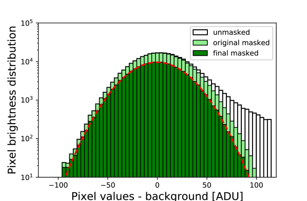
Figure 3: Distributions of background pixel values before masking (white bar), after the original masking (light green bar) and after expanded masking (green bar) are plotted. After the final masking, the pixel values show a Gaussian distribution (red dashed line) with improved skewness from 14.47 (before masking) to 0.02 (after original masking) and to 0.005 (after expanded masking).

Despite our rigorous masking procedure, there may remain diffuse light originating from the galaxy outskirts. Indeed, the pixels right outside of the mask appear to show some remaining light from the galaxies (see Figure 4). The light emanating close to the galaxies could also be partly composed of ICL; however, for a more conservative ICL detection, we will eliminate all of this light. We assume that there is no ICL outside the 300 kpc region, and proceed to check how large the mask should be to cover the remaining light from the galaxy outskirts.

Outside of the region of 300 kpc in the north-east half of the image, we select ten galaxies including three member galaxies and seven SDSS galaxies without spectroscopic redshift and measure the fluxes immediately outside their masked regions. We expand the mask in a pixel by pixel manner; i.e., pixels next to (left, right, up and down) the masked pixel will be masked in the next step. The advantage of this mask-expansion method is that we do not assume or model the shapes of the bright sources but expand the mask as it is in a shape-independent manner. The images in Figure 4 show how the remaining fluxes around an example galaxy are eliminated as the mask is enlarged from 0 pixels (original mask) to five pixels, ten pixels and finally to 15 pixels. Regarding the decision of the proper size of the mask which eliminates galaxy outskirt light safely while keeping enough pixels to analyse, we plot the radial profiles of the ten galaxies while applying each step of the enlarged mask. Reducing noise while preserving the overall signal tendency, we set the radial bin size to 8 and take the median value only if the remaining pixels exceed half of the pixels in the radial bin. We read out the first measured flux value for each mask-expanding step, i.e., the flux just outside of that mask, which is plotted with the grey lines in the bottom panel of Figure 4. The fits to the remaining fluxes of the ten galaxies are plotted with the red line. As expected, as the mask size grows as the remaining flux approaches the background value. After 15 steps of expanded masking, the fitting value is inside the background error, which is our detection limit. Thus, we decide to apply the 15 steps of expanded masking in our analysis. The final mask-applied postage stamp image in Figure 4 shows again that the residual light from galaxy outskirt is well removed. Assuming that the outskirt light sources of the galaxies in the central region fade out similarly, we apply this oversized mask to the entire image area.

It should be noted that the background value and corresponding error are affected by the mask size. We apply the expanded mask to measure the background value (see Section 3.3) and plot the remaining fluxes iteratively, which does not change the tendency. After applying the expanded mask, the pixel brightness distribution becomes even more Gaussian with skewness of 0.005 (see the dark green histogram and the red dashed line in Figure 3).

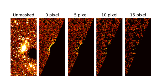
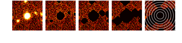
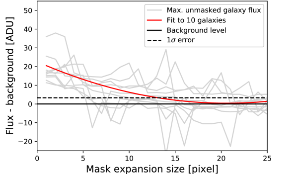
Figure 4: (Top) The i–band images for each masking step. The corresponding unmasked, original masked, five pixel expanded masked, ten pixel expanded masked and 15-pixel expanded masked images are shown in a row. (Middle) Stamp images of an example galaxy for each masking step, ordered as in the panel above. The radial bins used to measure the profile of the remaining light are denoted by the marked as white rings. (Bottom) Plot of the remaining light as the mask size expands. Ten galaxies are plotted as grey lines and the corresponding fit is plotted with the red line. The fitting line drops below the background error level from the 15-pixel enlarged mask, corresponding to the final mask size chosen. See more details about this method in Section 3.2.

3.3 Background level and error determination

Robust detection of ICL can be claimed only if we measure a significant ICL signal above the background fluctuation level. Thus, in this study the determination of the background level and the measurement of its noise are critical steps.

The characterization of the background and background noise is performed as follows. The final mask (as decided upon in Section 3.2) is applied to each band image. Outside the BCG’s 300 kpc region in the north-east half of the image, which we used as a background in the masking test (see the red defined region in Figure 1), we compute the median value of 30 $\times$ 30 pixels ($\sim$ 28.5 kpc; $\sim 4.8\arcsec$) grid boxes. The box size is tested while varying it from 1 $\times$ 1 pixel to 100 $\times$ 100 pixels, and is decided considering the apparent galaxy size in the image. Adopting the median values and the corresponding standard deviation, we find the background (12055.03 ADU for i–band, 5241.76 ADU for r–band) and its error (3.3 ADU for i–band, 2.23 ADU for r–band). In this study, we adopt these 1 $\sigma$ background uncertainties as the detection threshold of the ICL, which are $\mu_{i}^{limit}$(1$\sigma$, $4.8\arcsec\times 4.8\arcsec$) = 28.7 mag/arcsec² and $\mu_{r}^{limit}$(1$\sigma$, $4.8\arcsec\times 4.8\arcsec$) = 29.1 mag/arcsec².

We also conduct a test to compute the median of 30 $\times$ 30 pixels for 10,000 random positions. Because the random position measurement results in a slightly smaller background error, we decide to use the non-overlap grid background/background error measurement method to detect the ICL more conservatively. Furthermore, we split the background region and check if the background level changes depending on the distance to the BCG (see Table 3), and subsequently how this affects the surface brightness and colour profiles. We could not detect any trend on the background level related to the distance to the BCG. The different background levels for each radial bin lead to some changes of the ICL profile outside 155 kpc, but for the colour profile, they do not significantly affect the blue colour nor the steep profile (see Section 4.1).

Table 3: Background level and error in different regions

	i–band		r–band
Background	Background	Background	Background	Background
region	level	error	level	error
(kpc from centre)	[ADU]	[ADU]	[ADU]	[ADU]
All (300 $\sim$)c	12055.03	3.30	5241.76	2.23
300 $\sim$ 400	12052.63	3.24	5241.06	1.97
400 $\sim$ 500	12054.67	2.96	5242.25	1.27
500 $\sim$ 600	12056.92	3.17	5242.74	1.79
600 $\sim$ 700	12054.42	3.41	5240.53	2.66
c The All (300 $\sim$) corresponds to the red defined region in Figure 1.

We also estimated the surface brightness limit as suggested by Román et al. (2020), which results in a deeper limit of $\mu_{i}^{limit}$(1$\sigma$, $4.8\arcsec\times 4.8\arcsec$) = 30.19 mag/arcsec². The Gaussian standard deviation on a desired angular scale box is in this case converted from the pixel variation, assuming that the flux noise follows a normal distribution. In our case, the pixel variation (i.e., a 1 $\times$ 1 pixel grid box variation in the test above) is 1$\sigma_{pix}$ = 25.01 ADU (see the red dashed line in Figure 3). It should also be noted that our standard deviation is directly measured from boxes 30 $\times$ 30 pixels in size in the final reduced and masked image. For more conservative ICL measurements, we decide to use our method.

4 Results

Below we describe the ICL measurements in Section 4.1, after which we derive the properties of the galaxy cluster, the BCG and member galaxies thought to be related to the characteristics of the ICL in Sections 4.2, 4.3 and 4.4, respectively.

4.1 ICL measurements: surface brightness, colour, spatial distribution, fraction

In nearby clusters, ICL is studied typically below a surface brightness threshold of $\mu_{V}\sim$ 26.5 mag/arcsec² in the rest-frame (Mihos et al., 2005; Mihos et al., 2017; Rudick et al., 2011). This limit corresponds to $\mu_{i}\sim$ 27.18 mag/arcsec² and $\mu_{r}\sim$ 28.08 mag/arcsec² at $z=0.47$ considering the surface brightness dimming correction of $\sim{\color[rgb]{0,0,0}2.5}(1+z)^{{\color[rgb]{0,0,0}3}}$ and taking into account the stellar population evolution and the passband shift at the cluster redshift. These surface brightness limit conversions are calculated following equation (1) and (2) in Burke et al. (2015). Here, we used the stellar population synthesis models of Bruzual & Charlot (2003) while assuming the formation redshift of $z_{f}$ = 3, a simple stellar population with solar metallicity, and the initial mass function of Chabrier (2003). Thus, with our surface brightness limits ($\mu_{i}$ = 28.7 mag/arcsec² and $\mu_{r}$ = 29.1 mag/arcsec²), our Gemini images allow us to explore the ICL distribution out to $\sim$ 155 kpc (170 kpc) from the BCG for the i–band (r–band), as shown in Figure 5.

Surface brightness: In Figure 5, we plot the radial surface brightness profiles for the ICL as a function of the radius from the BCG. The radial profile is derived by taking the azimuthally averaged value of the remaining pixels in each bin after applying the mask. The inner radius was determined by locating the bin in which unmasked pixels start to dominate. Accordingly, the ICL profile does not have values in the central region of 60 kpc. The outer radius corresponds to the detection limit, 28.7 mag/arcsec², around 155 kpc in the i–band case. Therefore, the ICL analysis is conducted only in the range of 60 kpc and 155 kpc for both i– and r–band images.

We also plot the radial surface brightness profiles for the total cluster light together after masking out stars and non-member galaxies. We identify the spectroscopically confirmed member galaxies (see Section 4.2.1), after which the mask is expanded in the same way as the ICL. There may be more undetected member galaxies, possibly causing us to underestimate the total light. In fact, around 125 kpc and 195 kpc there is no member galaxy in the bin, which results in a drop of the total light. In contrast, the total light showed an excess level around 170 kpc due to several member galaxies in the bin.

The BCG-dominated central part of the total light is fitted as an s$\grave{e}$rsic profile with an s$\grave{e}$rsic index of n = 2 (further described in Section 4.3), whereas the ICL is better described by the s$\grave{e}$rsic model with n = 1 (Figure 5). This result suggests that the two components (BCG+ICL) have different physical origins (Cooper et al., 2015), where the outer component consists mainly of the ICL rather than the BCG. To disentangle the ICL from the BCG outskirt directly (i.e., to check if it follows the galaxy cluster potential or not), we need its spectroscopic data to measure the velocity dispersion, which was not possible in this study.

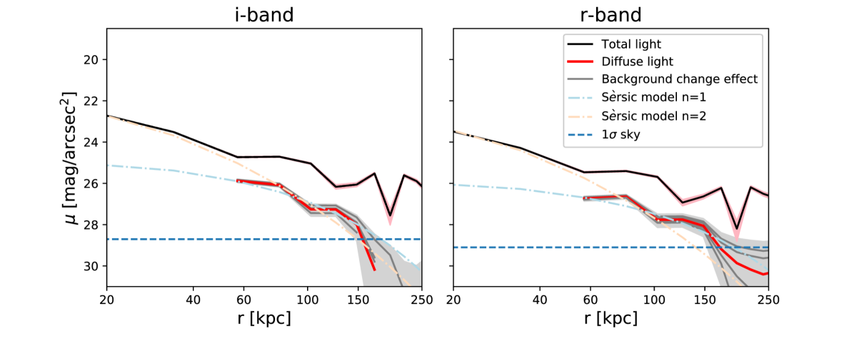
Figure 5: Radial surface brightness profiles for the i–band (left) and r–band (right). The mean value of each radial bin for total light (masking non-member galaxies and stars, and expanding the mask) and diffuse light (masking all bright objects, and expanding the mask) are plotted as black and red solid lines, respectively (see Sections 3.2 and 4.1 for details). For the i–band, the profile in the ranges, where the averaged fluxes have negative values with large uncertainties is not plotted. The s$\grave{e}$rsic models with s$\grave{e}$rsic indexes of n = 1 and 2 are plotted as the light blue and orange dot-dashed line, respectively. The 1$\sigma$ level detection limit is indicated by the blue dashed line, and the errors for total (diffuse) light are plotted as the filled pink (grey) regions. The effects of the background level changes (see the Table 3) on the diffuse light profiles are plotted as grey solid lines. The analysed radius range of the diffuse light starts from 60 kpc and ends by 155 kpc, where the i–band surface brightness profile touches the detection limit.

Colour: After identical masking, we created r–i colour profiles of the total light and ICL by subtracting the surface brightness profiles at the same radial bin in two bands (Figure 6), which corresponds to the B–V colour in the rest-frame. Regarding the error of the colour profile, we used the Monte-Carlo method based on the background estimates and uncertainty. As the Monte-Carlo estimated error of the colour profile becomes significantly larger in the outer radius, we do not trust the colour greater than $\sim$ 150 kpc. The choice of the background level (see the Table 3) varies the colour maximally around $\sim$ 0.2 in the range of 80 $\sim$ 130 kpc (see the grey solid lines in Figure 6), which does not significantly affect our results.

The colour of the diffuse light around 60 $\sim$ 80 kpc is similar to those of the BCG and bright red members. This might imply that diffuse light in the central region of the cluster is closely tied to the BCG and/or bright red members. The total light gradually becomes bluer beyond $\sim$ 70 kpc, but this trend appears to be steeper for the diffuse light. In the range of 80 $\sim$ 130 kpc, the ICL colour is r–i = 0.47 $\pm$ 0.28, whereas the total light colour is r–i = 0.68 $\pm$ 0.05. This difference might suggest that the main stellar population of the diffuse light is not likely to originate from that of the BCG and/or bright red members. In Section 5.1 we discuss the possible origins of the ICL further, specifically the relation between the colour of the ICL and that of the BCG/member galaxies and the colour evolution of the ICL.

For the total light, the spectroscopically confirmed member galaxies could be selectively red galaxies, as they are more likely to be brighter (more massive) red-sequence member galaxies and thus listed as a priority for many spectroscopic observations. This could bias the colour of the total light toward red. If we recalculate while including all detected galaxies, the colour of total light becomes r–i = 0.65 $\pm$ 0.04, which is still redder than the colour of the ICL.

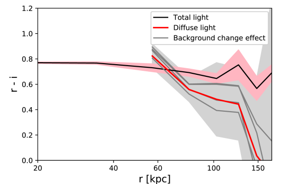
Figure 6: The r–i colour profile for the total light (black solid line) and diffuse light (red solid line). The definition of the total/diffuse light, the radial bin width, and the radius range are identical to those in Figure 5. The pink (grey) shaded regions show the Monte-Carlo errors of the r–i colour of the total (diffuse) light, based on the background uncertainty of each band. The effects of the background level changes (see the Table 3) on the colour profile of the diffuse light are plotted as grey solid lines. Up to 70 kpc, the colour of the diffuse light is similar to that of the total light, whereas outside of 80 kpc it becomes bluer than the total light, including the BCG and other nearby red member galaxies. The colour gradient of the diffuse light is steeper than that of the total light as well, but the errors are large and preclude definitive results.

Spatial distribution: The spatial distribution of the diffuse light is shown in Figure 7. Similar to the colour radial profile, subtracting the i–band surface brightness from the r–band gives us a two-dimensional colour map of the diffuse light. These surface brightness and colour 2D maps are smoothed by the Gaussian2DKernel astropy package with an oversampling factor of 17. Due to the masking and smoothing, some small parts of the central region in the 2D maps are not plotted. Both the i–band and r–band diffuse light distributions show a distinct elongated and tilted structure. This structure is visible in the r–i colour distribution as well. We compare it with the distribution of the member galaxies/luminosity-weighted distribution of member galaxies in Section 5.2.

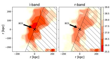
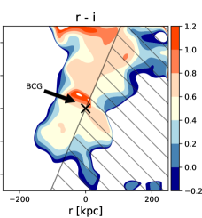
Figure 7: Diffuse light (after masking) surface brightness 2D map for the i–band (left) and r–band (middle) and the r–i colour 2D map (right) are plotted. The colour bar for the i–band and r–band 2D maps is located on the right side of the r–band 2D map, which has unit of mag/arcsec². The colour bar of r–i colour 2D map is on the right side of this map. The 2D maps are Gaussian smoothed using the Gaussian2DKernel astropy package with an oversampling factor of 17. The BCG centre location is marked. The hatched region on the south-west side is excluded during the ICL analysis. Both the i–band and the r–band diffuse light distributions show clear elongation and a tilted position angle.

ICL fraction: In Figure 8, we show the ICL fraction in the i–band (corresponds to the V–band in the rest-frame), defined as the ratio of the surface brightness of the ICL to the total light at the same radial bin. In order to measure the total cluster light, we mask out non-member galaxies and stars, as described earlier. Again, the lack of spectroscopically confirmed member galaxies in the bin around 125 kpc makes the total light lower and enhances the ICL fraction.

By making the bin range larger, in the range of 60 $\sim$ 155 kpc, we calculate an ICL fraction of J1054 is $15.07\pm 4.57\%$. The same calculation for the r–band gives an ICL fraction of $19.95\pm 5.67\%$. We could interpret this as a conservative estimation of the ICL fraction due to our rigorous expanding mask procedure to cover diffuse light that may belong to galaxies. However, the possible missing member galaxy light in this area would lead to an underestimation of the total light. Similarly, for the colour estimation, if we calculate the ICL fraction including all detected galaxies for the total light, the ICL fraction becomes $14.50\pm 4.4\%$ for the i–band, and $18.86\pm 5.36\%$ for the r–band, which could correspond to a lower limit of the ICL fraction for J1054.

We exclude the range of 0 $\sim$ 60 kpc when calculating the overall ICL fraction of J1054, where the abundance of ICL could not be estimated. In this range, the BCG light should be dominant, but at the same time, the ICL abundance is also expected to reach its maximum along the line of sight. Because separation between the ICL and the extended envelope of the BCG is photometrically impossible (as discussed in Gonzalez et al., 2007), to mitigate the uncertainty, we focus on the region where the ICL is more dominant. However, for comparisons with other studies, we calculate the ICL fraction using a surface brightness cut in the range 0 < r < $R_{500}$ (in Section 5.3), which results in a rather high ICL fraction of J1054.

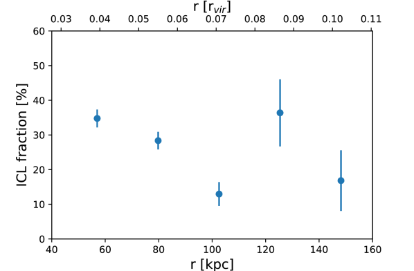
Figure 8: Radial ICL fraction calculated according to the ratio of the diffuse light to the total light. The radius in unit of the virial radius is shown in the upper axis. The background-variation-driven ICL fraction errors are marked as error bars. Through mask incompleteness correction (described in Section 3.2), we eliminated the possible remaining light from the galaxy outskirts.

4.2 Galaxy cluster properties

4.2.1 Member identification

The previous study of J1054 obtained 116 spectroscopic redshifts of galaxies, and of those 78 member galaxies were identified (Aguerri et al., 2011). Aguerri et al. used the shifting gapper method, which rejects galaxies with large peculiar velocities in fixed distance bins. We add three more redshifts from our MOS observation to the previous 116 and then re-select member galaxies using the Caustic method, which is a physically well-motivated technique (Serra & Diaferio, 2014). The Caustic method measures the escape velocity profiles of galaxy clusters and identifies member galaxies based on these profiles. In the Caustic method, we choose the Antonaldo Diaferio’s threshold (Diaferio, 1999) for cluster candidate members and fixed the centre as the BCG location, resulting in 73 newly selected member galaxies. Compared to the previous result with 78 members, our membership selection process is tighter and results in fewer member galaxies. Figure 9 shows a phase space diagram plotting the 119 galaxies with a spectroscopic redshift (line-of-sight velocities lower than -3500 km/s or higher than 5000 km/s are not plotted) as well as the corresponding escape-velocity-driven caustic profiles and selected member galaxies inside the caustic profile. The line-of-sight velocity of the selected member galaxies ranges from -1896 km/s to 1902 km/s, and the maximum projected distance from the corresponding BCG centre is 1.59 Mpc.

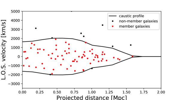
Figure 9: Phase space diagram of J1054. Among 119 candidate galaxies with spectroscopic redshifts, 73 member galaxies (red dots) are selected through the Caustic method. The calculated caustic profile from the velocity information of these 119 galaxies is plotted as the black solid line in the figure. Non-member galaxies with line-of-sight velocities of less than -3500 km/s or that exceed 5000 km/s are not plotted in this diagram.

4.2.2 Cluster mass and radius derivation

Using the velocity data of the identified member galaxies, the Caustic method provides a median redshift of $z=0.465729$ $\pm$ 0.003995, a median line-of-sight velocity of $v=139622.0$ $\pm$ 817.13 km/s, a rest-frame velocity dispersion $\sigma_{v}=934.36$ $\pm$ 13.20 km/s and $r_{200}=1.68$ $\pm$ 0.20 Mpc, $M_{200}={\color[rgb]{0,0,0}7.58\pm 1.40}\times 10^{14}M_{\odot}$ from fitting with an NFW profile. Those results are not far from those in a previous study (Aguerri et al., 2011) with 78 member galaxies. Again, this confirms that J1054 is an extremely rare target, being a fossil and massive cluster at an intermediate redshift level.

4.3 BCG properties

Our deep imaging observations of J1054’s BCG reveal a distinct structure that resembles a nearest neighbour (or accretion) approximately 10 kpc away from the BCG centre (see Figure 10). Its colour is identical to that of the BCG centre, which suggests that it is likely to belong to the cluster. Unfortunately, our MOS slit on the BCG does not go through this structure, meaning that we could not analyse its spectrum. Future spectroscopic studies on this structure would help to reveal its identity and the dynamic relation with the BCG.

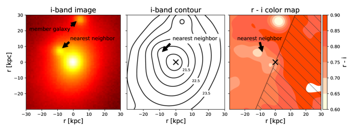
Figure 10: Stamp image (left), surface brightness contour in the i–band (middle) and r–i colour contour (right) of the BCG. The colour bar for the r–i colour is located on the right side of the contour map. The hatched region on the south-west side is excluded for the ICL analysis. The nearest neighbour of the BCG is detected at approximately10 kpc from the BCG centre. No spectroscopic redshift information exists for this structure, but it shows an r–i colour similar to that of the centre of the BCG.

The existence of this structure was not reported in a previous study of J1054 (Aguerri et al., 2011), though they report that the BCG does not have extra light outside and can be fitted as a single s$\grave{e}$rsic profile with an index of n $\sim$ 2.1, which means it is not a cD galaxy. They conclude that to have this low s$\grave{e}$rsic index as a luminous elliptical galaxy at this redshift, it should have undergone extreme wet merging ($\sim$ 80% gas rich). Using the Sersic1D astropy package, we measure the s$\grave{e}$rsic index of the observed BCG image with and without masking of the neighbour structure. We do not fit in the inner-most seeing-dominated region (Mahabal et al., 1999; Spavone et al., 2017) of the BCG inside nine kpc ($\sim$ 1.5 $\times$ FWHM). The resulting s$\grave{e}$rsic index is n = 2.21 $\pm$ 0.02 with the neighbour structure and n = 2.00 $\pm$ 0.02 without it, showing a minor difference.

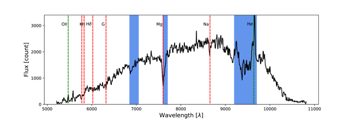
Figure 11: The BCG spectrum from the MOS observation is plotted. The green and red dashed lines are the emission and absorption lines for $z=0.468$, respectively. The blue filled regions are where the sky lines are located. Mg and Na absorption lines and a weak [OII] emission line are visible, but the H$\delta$ absorption line is negligible.

We analyse the BCG spectrum from the MOS observation (see Figure 11). Using the Mg and Na absorption lines and the weak [OII] emission line, we confirm its redshift as 0.468. The [OII] emission line is very weak and there is no visible H$\delta$ absorption line, which implies that there was no post-starburst activity within 1 Gyr. The strong H$\alpha$ emission line that appeared similarly in all observed galaxies is less reliable because it is located where sky lines exist. The r–i colour of the BCG is 0.89 $\pm$ 0.04 (MAG_AUTO of SExtractor from the observed Gemini image), which is comparable to those of other observed luminous red elliptical galaxies at $z\sim 0.47$ (r–i = 0.8/0.9 at $z\sim 0.45/0.5$; Maraston et al., 2009). We calculate its $D_{n}4000$ index following the definition of Balogh et al. (1999), which is the flux within a 100 Å window with a central wavelength of 4050 Å divided by the flux in a 100 Å window with a central wavelength of 3900 Å. The $D_{n}4000$ index of the BCG is 1.98 from our Gemini spectrum and 1.71 from the SDSS spectrum, which is higher or comparable to those of other passive luminous red galaxies with $D_{n}4000$ =1.75 (Roseboom et al., 2006) and meaning that the BCG of J1054 is composed of an older stellar population. We fitted the spectrum using CIGALE (Burgarella et al., 2005; Noll et al., 2009; Boquien et al., 2019), which estimates the BCG age to be 7 $\pm$ 0.5 Gyr.

We also check data from the Wide-field Infrared Survey Explorer (WISE; Wright et al., 2010), especially the w1mag [3.4$\mu$m] - w3mag [12$\mu$m] colour of the BCG, as the mid-infrared (mid-IR) colours of red early-type galaxies have strong correlations in age-sensitive spectral features, meaning that the mid-IR can be a useful diagnostic tool with which to assess the existence of young and intermediate-age stars (Ko et al., 2013; Ko et al., 2014; Ko et al., 2016). The mid-IR colour of the BCG is 1.197, which is at least one magnitude bluer than other member galaxies. Thus, we could conclude that the contribution of the young stellar population within the BCG of J1054 is negligible. Considering the nearest neighbour, the BCG of J1054 seems to have undergone dry merging without recent significant star formation.

4.4 Member galaxies properties

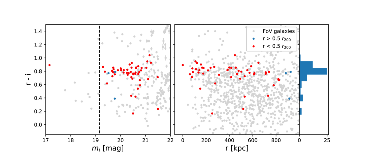
Figure 12: (Left) r–i colour vs. the i–band magnitude for all galaxies (grey dots) within the Gemini field of view in the J1054 field. Among the 73 member galaxies, 53 are detected within the Gemini field of view and are indicated here by the red and blue dots. Red dots are members within 0.5 $r_{200}$ (840 kpc) from the BCG centre, while blue dots are members outside of 0.5 $r_{200}$. The dashed line is where the magnitude is $m_{BCG}+2$, showing that J1054 fulfils the criteria to be recognised as a fossil cluster. The r–i colour errors are indicated by the grey errorbar. (Right) r–i colour distribution for 53 members and field of view galaxies as a function of the radial distance from the BCG. The histogram on the right side represents the colour distribution of the 53 member galaxies. The BCG and red sequence galaxies of J1054 have r–i colour values of 0.7 $\sim$ 0.9, and the overall colour values of the member galaxies range widely from 0.17 to 1.04.

The colour and spatial distribution of cluster galaxies could help us to constrain the ICL formation mechanism. We identified 73 cluster member galaxies of J1054 in Section 4.2.1. Among the member galaxies, 53 galaxies are detected within the full field of view of the Gemini images. In Figure 12, the colour-magnitude diagram of the member galaxies confirms again that J1054 fulfils the definition of a fossil cluster with a magnitude gap of 2.14 between the BCG and the second brightest galaxy within half of the projected virial radius ($\sim r_{200}$ = 1.68 Mpc). The actual second brightest member galaxy (magnitude gap from the BCG is 1.56 in the modelMag from SDSS DR16) is 1271 kpc away from the BCG.

The colour distribution of the member galaxies shows a narrow red sequence with an r–i colour of $\sim$ 0.8, and a wide range of blue galaxies to $\sim$ 0.2 (Figure 12). As expected from a dynamically relaxed cluster, bright red galaxies are dominant in the central region, and faint blue galaxies tend to be located in the outer region of the cluster.

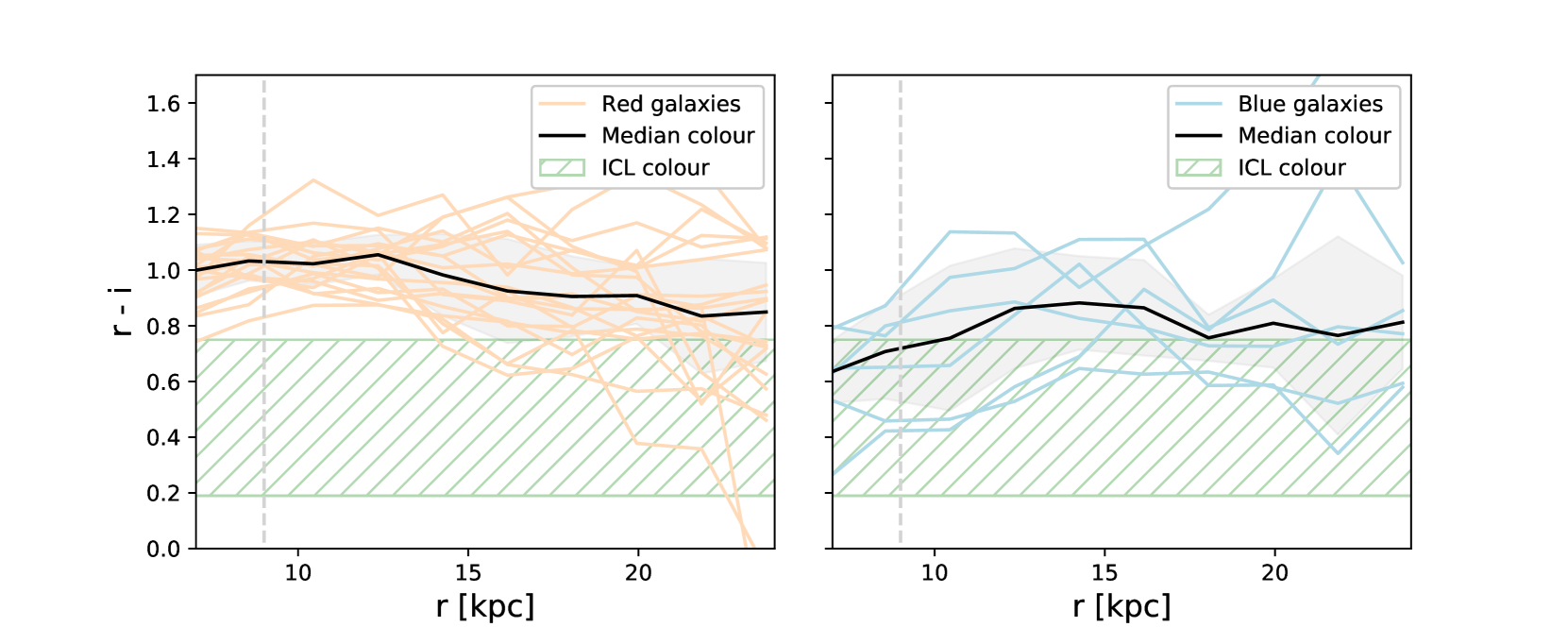
Figure 13: The r–i colour profiles of 21 red sequence galaxies (left) and six blue galaxies (right) are plotted. The black solid lines represent the median colour profiles. The 1$\sigma$ scatter outcomes of the profiles are plotted as the filled grey region in both panels (we clipped the 2$\sigma$ outlier data points due to the sparsity of the sample set). We consider only points outside of the radius of approximately 1.5$\arcsec$ (grey dashed line) to avoid the seeing effect. For comparison, the r–i colours of ICL (0.47 $\pm$ 0.28 in the range of 80 $\sim$ 130 kpc) are indicated (green hatched region) in both panels.

We also checked the r–i colour radial profile of 27 member galaxies (except the BCG) in our full-exposure image area. First, we classify 21 red galaxies (r–i $\geq$ 0.75) and six blue galaxies (r–i $<$ 0.75). The magnitude ranges for the red and blue galaxies are $19.30<m_{i}<21.28$ and $19.47<m_{i}<20.63$, respectively. Figure 13 shows the median colour profiles of the red galaxies (left panel) and the blue galaxies (right panel). The 1 $\sigma$ scatter in the profiles is plotted in each case as the filled grey region in each panel. In the same manner as the BCG radial profile, we avoid the central region of approximately 1.5$\arcsec$ ($\sim$ 9 kpc) which is affected by the seeing effect. Compared to the ICL colour, which is 0.47 $\pm$ 0.28 in the radial range of 80 $\sim$ 130 kpc, the colour of the ICL appears to be related to the outskirts (r $>$ 20 kpc) of the red/blue members and the core of the blue members.

5 Discussion

Based on the results from the ICL measurements and physical properties of the cluster, we discuss how the ICL is connected to the BCG, member galaxies and the host galaxy cluster.

5.1 What can the colour of ICL tell about the origin of ICL?

It is well known that the distribution of cluster galaxies in an optical colour-magnitude diagram is bimodal; quiescent, bright galaxies populate a narrow red sequence and star-forming, faint galaxies form a wide blue cloud (e.g., Strateva et al., 2001; Blanton et al., 2003; Baldry et al., 2004; Balogh et al., 2004; Choi et al., 2007; Ko et al., 2013). The ICL colour measurement compared to the colour distribution of cluster galaxies thus allows us to constrain the progenitor galaxies of the intracluster stars.

In the range of 80 $\sim$ 130 kpc, the ICL colour is r–i = 0.47 $\pm$ 0.28, where the BCG-dominated total light colour is r–i = 0.68 $\pm$ 0.05 (Figure 6). Moreover, the colour of the BCG is even redder (r–i = 0.89 $\pm$ 0.04), which is consistent with the estimated age ($\sim$ 7 $\pm$ 0.5 Gyr) from the BCG spectrum. This colour difference suggests that the main component of the ICL differs from that of the BCG and bright red galaxies. Rather, the colour of the ICL is similar to the outskirts of the red and/or blue member galaxies or the core of the bluest member (Figure 13). Furthermore, the colour gradient of the ICL appears to be negatively steeper than the total light with the large errors. This might indicate that intracluster stars in the central region are older and/or richer in metals than those in the outer part. This is consistent with previous ICL studies of similar redshifts ($z\sim 0.45$; Presotto et al., 2014; DeMaio et al., 2015; DeMaio et al., 2018). Presotto et al. (2014) reported that the ICL colour is similar to the envelope of the BCG rather than to the corresponding centre, and DeMaio et al. (2018) reported that the ICL colour within 100 kpc is consistent with red sequence galaxies but that it also has a negative gradient at 53 $\sim$ 100 kpc.

These results favour mechanisms according to which the ICL is not generated during the BCG major mergers at early times but are rather gradually accreted by tidal stripping of satellite/infalling galaxies. Similarly, a previous ICL study of the Virgo cluster (Mihos et al., 2017) reported the colour of a diffuse plume structure being B–V = 0.5 $\sim$ 0.6, which was explained as young stars being stripped from the disk of the galaxy or induced recent star formation in the tidal feature. It is also necessary to consider the colour evolution of the ICL as well. Contini et al. (2019) predicted that the ICL colour has a redshift evolution, i.e., B–V = 0.77 at $z=0$ and 0.63 at $z=1$. Moreover, several observational studies have shown that the ICL during intermediate redshifts is younger than those nearby (Toledo et al., 2011; Montes & Trujillo, 2014, 2018; Adami et al., 2016; Morishita et al., 2017; Jiménez-Teja et al., 2018). Therefore, the overall bluer r–i (B–V in the rest-frame) colour of the ICL at $z=0.47$, compared to the Virgo cluster (B–V = 0.7 $\sim$ 1.0; Rudick et al., 2010; Mihos et al., 2017), is comprehensible.

5.2 Does the spatial distribution of ICL follow that of the cluster galaxies?

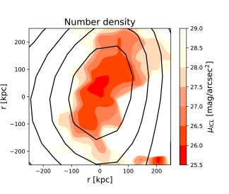
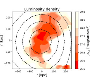
Figure 14: Contour of the galaxy number density map (left, black solid line) and contour of the luminosity-weighted number density map (right, black dashed line), over-plotted on the i–band diffuse light surface brightness 2D map. The 73 member galaxies are selected using the Caustic method (see Section 4.2.1). Their spatial distribution results in the number density map, and assigning weight to it using their i–band luminosity results in the luminosity density map. Because J1054 is a BCG-dominated fossil cluster, we associate the number density map with the member-galaxy-oriented ICL formation scenario, and the luminosity density map with the BCG-oriented scenario. Despite the fact that the number density map is generated using the location data of member galaxies in the SDSS catalogue, which is independent of our observational image data, the shape coincides with the diffuse light distribution. The measured ellipticities of the three innermost contours are 0.71, 0.66, and 0.64 for the number density, and 0.0, 0.49, and 0.49 for the luminosity density. The position angle is measured in degrees counter-clockwise from the vertical axis of the image (see Section 5.2 for details).

The spatial distribution of cluster member galaxies can be visualised as a galaxy number density map. Using the additional luminosity information (i–band magnitudes from SDSS) of each galaxy gives us a galaxy luminosity density map (Figure 14). We generate the 2D projected density maps on a 30 $\times$ 30 pixels binned grid over the spatial range where the 73 member galaxies reside and conduct Gaussian smoothing of each field with a factor of 2.2.

In Figure 14, the contours for the number density (derived from the positions of the galaxies) are elongated, whereas those for the luminosity-weighted density are rather more circular. The measured ellipticities of the three innermost contours are 0.71 $\pm$0.09, 0.66 $\pm$0.05, and 0.64 $\pm$0.04 for the number density and 0.0 $\pm$0.08, 0.49 $\pm$0.18, and 0.49 $\pm$0.10 for the luminosity density. Regarding the orientation, the measured position angles (in degrees counter-clockwise from the vertical axis of the image) of the three innermost contours are -75.10 $\pm$ 9.74°, -70.51 $\pm$ 7.45°, and -81.40 $\pm$ 38.96° for the number density, and 44.71 $\pm$ 10.31°, 63.06 $\pm$ 42.40°, and -82.55 $\pm$ 40.11° for the luminosity density. Because the luminosity density map is derived from the positions and luminosities of the cluster member galaxies, it does not take into account the shape of the BCG itself. The ellipticity of the BCG is 0.264 $\pm$ 0.001 and the corresponding position angle is -18.33 $\pm$ 0.09°, providing better agreement with the luminosity density map than with the number density map.

In the luminosity density contours, which draw concentric circles (right panel of Figure 14), we can clearly see J1054’s characteristic as a fossil cluster with dominating BCG. The number density map is closely linked to the cluster member galaxies, whereas the luminosity density map is more related to the luminosity-dominating BCG. Comparing the number and luminosity density maps with the ICL map may provide a hint to the origin of ICL. Regarding the elongated (ellipticity of 0.95 $\pm$ 0.02) and tilted (position angle of -74.20 $\pm$ 1.08°) shape, the ICL map is better matched (overlap at the 2 $\sigma$ level) to the galaxy number density map rather than to the luminosity-weighted density map, which implies that the ICL distribution is related more to cluster galaxies than solely to the BCG. We note that the outer region of cluster galaxies, if not adequately masked, may artificially induce a spatial correlation between the member galaxies and the ICL. In order to mitigate this risk, we masked luminous objects to measure the ICL in a conservative manner.

5.3 How abundant is the ICL of J1054 compared to that of other galaxy clusters?

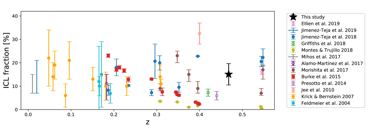
Figure 15: Reference ICL fractions of galaxy clusters in various redshifts using various ICL detection techniques. The ICL fraction of J1054 ($15.07\pm 4.57\%$) is indicated by the black star. Because these results are derived through different ICL defining methods, a comparison between ICL fractions should be done with caution. The results from Burke et al. (marked as red squares) are derived from surface brightness cuts as conducted in this study (see details in Section 5.3).

Investigating the ICL fraction allows us a further important constraint on the ICL formation and evolution processes. If intracluster stars in nearby galaxy clusters have been stripped from the cluster galaxies through numerous galaxy interactions, we can predict that the ICL fraction over a sample of galaxy clusters is closely related to redshift and dynamic state. Recent simulations show a strong evolution of the ICL fraction with the redshift (Rudick et al., 2011; Contini et al., 2014; Cooper et al., 2015). For example, Rudick et al. (2011) predicted via a simulation that the ICL fraction increases from $6.0\sim 8.5\%$ at $z=0.5$ to $9.5\sim 13.2\%$ at $z=0$, using a surface brightness threshold of $\mu_{V}$ = 26.5 mag/arcsec².

However, observational studies overall do not yet appear to support these simulation results. Figure 15 shows our ICL fraction measured in J1054 along with those in other clusters with varying redshifts. There does not appear to be a clear trend between the ICL fraction and the redshift. However, there are several ambiguities present. First, a common ICL detection method is lacking. The methods known thus far are as follows. Presotto et al. (2014), Alamo-Martínez & Blakeslee (2017), Morishita et al. (2017) and Griffiths et al. (2018) modelled galaxies using GALFIT and used this model to subtract the BGC and galaxy light contributions. They defined the ICL as the residual light after the removal of all light contributions of galaxies. Adami et al. (2016) and Ellien et al. (2019) used a wavelet-based method to model the surface brightness distribution of all galaxies, subtracting them to obtain the residual ICL map. Jiménez-Teja et al. (2018, 2019) used the CICLE method which is similar to the wavelet method. Feldmeier et al. (2004), Krick & Bernstein (2007), Jee (2010), Burke et al. (2012); Burke et al. (2015) Mihos et al. (2017), and Montes & Trujillo (2018) and this study use the surface brightness threshold. For example, Burke et al. (2015) (as indicated by the red squares in Figure 15) show a clear tendency of the ICL fraction increasing with a decrease in the redshift, whereas the data of Jimenez-Teja et al. and Morishita et al. (indicated by the filled circles) do not show any relation between the ICL fraction and the redshift. Second, the measurement technique for the ICL fraction (i.e. how to quantify the total cluster and ICL light) is different in each study. Montes & Trujillo (2018) demonstrated how the different definitions of the ICL affect the ICL fraction. Thus, it is difficult directly to compare multiple observational studies. To address this issue, we attempt to compare the results from the method adopted in this study. Compared to Burke et al. (the red square symbols), where a surface brightness threshold technique was used for the ICL measurement, J1054 appears to have a higher ICL fraction ($15.07\pm 4.57\%$ in the i–band which corresponds to a V–band in the rest-frame, black star symbol in Figure 15). Even if we take the lower limit ($14.50\pm 4.40\%$ in the i–band, calculated in Section 4.1), the ICL fraction of J1054 is still higher than that of the clusters in Burke et al.

A direct comparison of the ICL fraction measurement method of Burke et al. with our data is not possible, as their lower limit of the surface brightness is 26.4 mag/arcsec² (in the F625W filter), which is brighter than the ICL surface brightness threshold of 26.67 mag/arcsec² in the r–band (converted from 25 mag/arcsec² in the rest-frame B–band). If we take our r–band detection limit of 29.1 mag/arcsec² as the lower limit, adopting their radius limit ($R_{500}$) and their point source/non-cluster galaxy masking, which was enlarged by 1.5 times, the calculated ICL fraction (ICL over the total cluster light of BCG + ICL + satellite galaxies) of J1054 becomes even higher, at 19.77%, due to our deeper detection limit. Note that, as Burke et al. has already pointed out, their ICL fraction varies significantly with the lower limit of the surface brightness. Rudick et al. (2011) simulated the redshift evolution of the ICL fraction for various surface brightness thresholds (see their Figure 4) and predicted that the contribution of ICL dimmer than $\mu_{V}\sim$ 26.5 mag/arcsec² at $z\sim 0.47$ is about $\sim$ 8.5%. Because the lower limit of their simulated surface brightness is much deeper than current observations allow (reaching as low as $\mu_{V}=$ 35 mag/arcsec²), we may regard the ICL fraction of $\sim$ 8.5% as the amount of missing ICL due to the shallower detection limit relative to that surface brightness level. Thus, if our detection limit were as shallow as that of Burke et al., we would have missed that corresponding amount of ICL as well. If we accept this assumption, the estimated ICL fraction of J1054 according to the method by Burke et al. decreases to $\sim$ 11.27%, which still appears to be high for their ICL fraction-redshift relation.

Abell 2261 is one of the sample clusters of Burke et al., which is also a massive fossil cluster with $M_{vir}\sim 1.76\times 10^{15}M_{\odot}$(Merten et al., 2015). Considering its ICL fraction of $16.64\pm 0.78\%$ (Burke et al., 2015) at $z=0.22$ and the converted ICL fraction of J1054, of $\sim$ 11.27% at $z=0.47$, the growth factor over the corresponding redshift range is $\sim$ 1.48, which is likely to be consistent with simulation studies (Rudick et al., 2011; Contini et al., 2014). Rudick et al. predicted a factor of $\sim$ 1.35 and Contini et al. predicted factors of $\sim$ 1.47 and $\sim$ 1.56 for a tidal model with and without a merger channel, respectively. Among the various ICL growth mechanisms simulated by Contini et al. (see their Figure 6), the model with constant stripping and a merger channel (i.e., both the main mechanisms at play) matches our estimation of ICL growth best.

Assuming that fossil clusters at $0.4<z<0.5$ have BCGs whose formations have already finished, and further positing that a BCG major merger is the main ICL production mechanism, this would imply that most of the ICL would have been generated up until that epoch. From this point of view, our high ICL fraction could support the BCG origin scenario, whereas it is also an expected result from a fossil cluster, which is a dynamically mature system where galaxy-galaxy interactions such as tidal stripping have already taken place. Moreover, the bluer ICL colour compared to the BCG and the spatial distribution of the ICL aligned with member galaxies strengthen the possibility that J1054 has a fraction of its ICL component generated by stripping processes.

6 Conclusions

We have presented an ICL study of J1054, a massive fossil cluster at $z=0.47$, to improve constraints on the ICL formation mechanism. Gemini deep imaging and MOS observations were conducted to detect the diffuse ICL features of J1054 and investigate its connection with the BCG and cluster galaxies. Our imaging data reach to a very low surface brightness (29.1 and 28.7 mag/arcsec² for the r and i–band, respectively), sufficient for explorations of the ICL feature out to 155 kpc.

The ICL colour is bluer than the BCG and bright, red cluster galaxies beyond 70 kpc from the location of the BCG, and its colour gradient appears to be steeper than the total light with the large errors (Figure 6). The blue colour (r–i = 0.47 $\pm$ 0.28) of the ICL in the outer region (80 $\sim$ 130 kpc) disfavours the ICL formation mechanism related to major mergers, including those associated with the BCG. Instead, our findings may support mechanisms produced by the recent stripping of the outskirts of infalling/satellite galaxies.

When comparing the spatial distribution of the ICL with cluster galaxies, we find that it is more likely to match the number density map rather than the luminosity-weighted density map (Figure 14), which implies that the ICL distribution is related more to member galaxies than solely to the BCG.

We estimate an ICL fraction of $15.07\pm 4.57\%$ in the range of $60\sim 155$ kpc, which appears higher than the ICL fraction-redshift trend reported by Burke et al. (Figure 15). Converting the ICL fraction of J1054 to match the detection limit in Burke et al. and comparing it with the ICL fraction of a massive fossil cluster sample, Abell 2261, at $z=0.22$, the estimated growth factor for this redshift interval appears to be consistent with the tidal stripping $+$ merger model of Contini et al. (2014).

Describing the ICL formation process of J1054 through a single mechanism may not be sufficient. Ideally, we would require a sample of massive fossil clusters with varying redshifts to draw a firm conclusion about the dominant ICL formation mechanism during the hierarchical growth of the cluster. Obtaining high-z ($z\geq 1$) fossil cluster samples in future surveys, such as the Vera C. Rubin Observatory’s Legacy Survey of Space and Time (LSST) would be particularly helpful regarding the early BCG build-up and late ($z<1$) tidal stripping ICL production scenario. Furthermore, a detailed analysis on the ICL colour, spatial distribution and fraction in the sample will help to constrain the model to the origin of the ICL.

Data Availability

The data underlying this article are available in the Gemini Observatory Archive at https://archive.gemini.edu/searchform, and can be accessed with Program ID:GN-2018A-Q-201/PI:Jaewon Yoo.

References

- Abazajian et al. (2004) Abazajian K., et al., 2004, AJ, 128, 502
- Abolfathi et al. (2018) Abolfathi B., et al., 2018, ApJS, 235, 42
- Adami et al. (2016) Adami C., et al., 2016, A&A, 592, A7
- Adelman-McCarthy et al. (2007) Adelman-McCarthy J. K., et al., 2007, ApJS, 172, 634
- Aguado et al. (2019) Aguado D. S., et al., 2019, ApJS, 240, 23
- Aguerri et al. (2011) Aguerri J. A. L., et al., 2011, A&A, 527, A143
- Alamo-Martínez & Blakeslee (2017) Alamo-Martínez K. A., Blakeslee J. P., 2017, ApJ, 849, 6
- Alonso Asensio et al. (2020) Alonso Asensio I., Dalla Vecchia C., Bahé Y. M., Barnes D. J., Kay S. T., 2020, MNRAS, 494, 1859
- Arnaboldi & Gerhard (2010) Arnaboldi M., Gerhard O., 2010, Highlights of Astronomy, 15, 97
- Astropy Collaboration et al. (2013) Astropy Collaboration et al., 2013, A&A, 558, A33
- Baldry et al. (2004) Baldry I. K., Glazebrook K., Brinkmann J., Ivezić Ž., Lupton R. H., Nichol R. C., Szalay A. S., 2004, ApJ, 600, 681
- Balogh et al. (1999) Balogh M. L., Morris S. L., Yee H. K. C., Carlberg R. G., Ellingson E., 1999, ApJ, 527, 54
- Balogh et al. (2004) Balogh M., et al., 2004, MNRAS, 348, 1355
- Barden et al. (2012) Barden M., Häußler B., Peng C. Y., McIntosh D. H., Guo Y., 2012, MNRAS, 422, 449
- Bertin (2011) Bertin E., 2011, in Evans I. N., Accomazzi A., Mink D. J., Rots A. H., eds, Astronomical Society of the Pacific Conference Series Vol. 442, Astronomical Data Analysis Software and Systems XX. p. 435
- Bertin & Arnouts (1996) Bertin E., Arnouts S., 1996, A&AS, 117, 393
- Blanton et al. (2003) Blanton M. R., et al., 2003, ApJ, 594, 186
- Boquien et al. (2019) Boquien M., Burgarella D., Roehlly Y., Buat V., Ciesla L., Corre D., Inoue A. K., Salas H., 2019, A&A, 622, A103
- Borlaff et al. (2019) Borlaff A., et al., 2019, A&A, 621, A133
- Bruzual & Charlot (2003) Bruzual G., Charlot S., 2003, MNRAS, 344, 1000
- Buote et al. (2016) Buote D. A., Su Y., Gastaldello F., Brighenti F., 2016, ApJ, 826, 146
- Burgarella et al. (2005) Burgarella D., Buat V., Iglesias-Páramo J., 2005, MNRAS, 360, 1413
- Burke et al. (2012) Burke C., Collins C. A., Stott J. P., Hilton M., 2012, MNRAS, 425, 2058
- Burke et al. (2015) Burke C., Hilton M., Collins C., 2015, MNRAS, 449, 2353
- Capaccioli et al. (2015) Capaccioli M., et al., 2015, A&A, 581, A10
- Chabrier (2003) Chabrier G., 2003, PASP, 115, 763
- Choi et al. (2007) Choi Y.-Y., Park C., Vogeley M. S., 2007, ApJ, 658, 884
- Chonis & Gaskell (2008) Chonis T. S., Gaskell C. M., 2008, AJ, 135, 264
- Conroy et al. (2007) Conroy C., Wechsler R. H., Kravtsov A. V., 2007, ApJ, 668, 826
- Contini et al. (2014) Contini E., De Lucia G., Villalobos Á., Borgani S., 2014, MNRAS, 437, 3787
- Contini et al. (2019) Contini E., Yi S. K., Kang X., 2019, ApJ, 871, 24
- Cooper et al. (2015) Cooper A. P., Gao L., Guo Q., Frenk C. S., Jenkins A., Springel V., White S. D. M., 2015, MNRAS, 451, 2703
- Csabai et al. (2007) Csabai I., Dobos L., Trencséni M., Herczegh G., Józsa P., Purger N., Budavári T., Szalay A. S., 2007, Astronomische Nachrichten, 328, 852
- Cypriano et al. (2006) Cypriano E. S., Mendes de Oliveira C. L., Sodré Laerte J., 2006, AJ, 132, 514
- D’Onghia et al. (2005) D’Onghia E., Sommer-Larsen J., Romeo A. D., Burkert A., Pedersen K., Portinari L., Rasmussen J., 2005, ApJ, 630, L109
- DeMaio et al. (2015) DeMaio T., Gonzalez A. H., Zabludoff A., Zaritsky D., Bradač M., 2015, MNRAS, 448, 1162
- DeMaio et al. (2018) DeMaio T., Gonzalez A. H., Zabludoff A., Zaritsky D., Connor T., Donahue M., Mulchaey J. S., 2018, MNRAS, 474, 3009
- Diaferio (1999) Diaferio A., 1999, MNRAS, 309, 610
- Duc et al. (2015) Duc P.-A., et al., 2015, MNRAS, 446, 120
- Ellien et al. (2019) Ellien A., Durret F., Adami C., Martinet N., Lobo C., Jauzac M., 2019, A&A, 628, A34
- Feldmeier et al. (2002) Feldmeier J. J., Mihos J. C., Morrison H. L., Rodney S. A., Harding P., 2002, ApJ, 575, 779
- Feldmeier et al. (2004) Feldmeier J. J., Mihos J. C., Morrison H. L., Harding P., Kaib N., Dubinski J., 2004, ApJ, 609, 617
- Furnell et al. (2021) Furnell K. E., et al., 2021, MNRAS, 502, 2419
- Galametz et al. (2013) Galametz A., et al., 2013, ApJS, 206, 10
- Gerhard et al. (2002) Gerhard O., Arnaboldi M., Freeman K. C., Okamura S., 2002, ApJ, 580, L121
- Gonzalez et al. (2005) Gonzalez A. H., Zabludoff A. I., Zaritsky D., 2005, ApJ, 618, 195
- Gonzalez et al. (2007) Gonzalez A. H., Zaritsky D., Zabludoff A. I., 2007, ApJ, 666, 147
- Green et al. (2019) Green G. M., Schlafly E., Zucker C., Speagle J. S., Finkbeiner D., 2019, ApJ, 887, 93
- Gregg & West (1998) Gregg M. D., West M. J., 1998, Nature, 396, 549
- Griffiths et al. (2018) Griffiths A., et al., 2018, MNRAS, 475, 2853
- Hook et al. (2004) Hook I. M., Jørgensen I., Allington-Smith J. R., Davies R. L., Metcalfe N., Murowinski R. G., Crampton D., 2004, PASP, 116, 425
- Iodice et al. (2017) Iodice E., et al., 2017, ApJ, 851, 75
- Jee (2010) Jee M. J., 2010, ApJ, 717, 420
- Jiménez-Teja et al. (2018) Jiménez-Teja Y., et al., 2018, ApJ, 857, 79
- Jiménez-Teja et al. (2019) Jiménez-Teja Y., et al., 2019, A&A, 622, A183
- Jones et al. (2003) Jones L. R., Ponman T. J., Horton A., Babul A., Ebeling H., Burke D. J., 2003, MNRAS, 343, 627
- Karabal et al. (2017) Karabal E., Duc P. A., Kuntschner H., Chanial P., Cuillandre J. C., Gwyn S., 2017, A&A, 601, A86
- Kluge et al. (2020) Kluge M., et al., 2020, ApJS, 247, 43
- Ko & Jee (2018) Ko J., Jee M. J., 2018, ApJ, 862, 95
- Ko et al. (2013) Ko J., Hwang H. S., Lee J. C., Sohn Y.-J., 2013, ApJ, 767, 90
- Ko et al. (2014) Ko J., Hwang H. S., Im M., Le Borgne D., Lee J. C., Elbaz D., 2014, ApJ, 791, 134
- Ko et al. (2016) Ko J., Chung H., Hwang H. S., Lee J. C., 2016, ApJ, 820, 132
- Krick & Bernstein (2007) Krick J. E., Bernstein R. A., 2007, AJ, 134, 466
- Lin & Mohr (2004) Lin Y.-T., Mohr J. J., 2004, ApJ, 617, 879
- Lin et al. (2017) Lin Y.-T., et al., 2017, ApJ, 851, 139
- Mahabal et al. (1999) Mahabal A., Kembhavi A., McCarthy P. J., 1999, ApJ, 516, L61
- Maraston et al. (2009) Maraston C., Strömbäck G., Thomas D., Wake D. A., Nichol R. C., 2009, MNRAS, 394, L107
- Masters & Capak (2011) Masters D., Capak P., 2011, PASP, 123, 638
- McGee & Balogh (2010) McGee S. L., Balogh M. L., 2010, MNRAS, 403, L79
- Merten et al. (2015) Merten J., et al., 2015, ApJ, 806, 4
- Mihos (2016) Mihos J. C., 2016, in The General Assembly of Galaxy Halos: Structure, Origin and Evolution. pp 27–34 (arXiv:1510.01929), doi:10.1017/S1743921315006857
- Mihos et al. (2005) Mihos J. C., Harding P., Feldmeier J., Morrison H., 2005, ApJ, 631, L41
- Mihos et al. (2017) Mihos J. C., Harding P., Feldmeier J. J., Rudick C., Janowiecki S., Morrison H., Slater C., Watkins A., 2017, ApJ, 834, 16
- Montes (2019) Montes M., 2019, arXiv e-prints, p. arXiv:1912.01616
- Montes & Trujillo (2014) Montes M., Trujillo I., 2014, ApJ, 794, 137
- Montes & Trujillo (2018) Montes M., Trujillo I., 2018, MNRAS, 474, 917
- Montes & Trujillo (2019) Montes M., Trujillo I., 2019, MNRAS, 482, 2838
- Montes et al. (2021) Montes M., Brough S., Owers M. S., Santucci G., 2021, ApJ, 910, 45
- Morishita et al. (2017) Morishita T., Abramson L. E., Treu T., Schmidt K. B., Vulcani B., Wang X., 2017, ApJ, 846, 139
- Murante et al. (2007) Murante G., Giovalli M., Gerhard O., Arnaboldi M., Borgani S., Dolag K., 2007, MNRAS, 377, 2
- Noll et al. (2009) Noll S., Burgarella D., Giovannoli E., Buat V., Marcillac D., Muñoz-Mateos J. C., 2009, A&A, 507, 1793
- Pierini et al. (2011) Pierini D., et al., 2011, MNRAS, 417, 2927
- Planck Collaboration et al. (2016) Planck Collaboration et al., 2016, A&A, 594, A10
- Ponman et al. (1994) Ponman T. J., Allan D. J., Jones L. R., Merrifield M., McHardy I. M., Lehto H. J., Luppino G. A., 1994, Nature, 369, 462
- Presotto et al. (2014) Presotto V., et al., 2014, A&A, 565, A126
- Puchwein et al. (2010) Puchwein E., Springel V., Sijacki D., Dolag K., 2010, MNRAS, 406, 936
- Purcell et al. (2007) Purcell C. W., Bullock J. S., Zentner A. R., 2007, ApJ, 666, 20
- Rines et al. (2007) Rines K., Finn R., Vikhlinin A., 2007, ApJ, 665, L9
- Rix et al. (2004) Rix H.-W., et al., 2004, ApJS, 152, 163
- Román et al. (2020) Román J., Trujillo I., Montes M., 2020, A&A, 644, A42
- Roseboom et al. (2006) Roseboom I. G., et al., 2006, MNRAS, 373, 349
- Rudick et al. (2010) Rudick C. S., Mihos J. C., Harding P., Feldmeier J. J., Janowiecki S., Morrison H. L., 2010, ApJ, 720, 569
- Rudick et al. (2011) Rudick C. S., Mihos J. C., McBride C. K., 2011, ApJ, 732, 48
- Santos et al. (2007) Santos W. A., Mendes de Oliveira C., Sodré Laerte J., 2007, AJ, 134, 1551
- Serra & Diaferio (2014) Serra A. L., Diaferio A., 2014, in The Caustic App v1.2 - Ana Laura Serra & Antonaldo Diaferio.
- Shaw (2016) Shaw R. A., 2016, in GMOS Data Reduction Cookbook (Version 1.2; Tucson: National Optical Astronomy Observatory), available online at: http://ast.noao.edu/sites/default/files/GMOS_Cookbook/.
- Spavone et al. (2017) Spavone M., et al., 2017, A&A, 603, A38
- Strateva et al. (2001) Strateva I., et al., 2001, AJ, 122, 1861
- Tavasoli et al. (2011) Tavasoli S., Khosroshahi H. G., Koohpaee A., Rahmani H., Ghanbari J., 2011, PASP, 123, 1
- Toledo et al. (2011) Toledo I., Melnick J., Selman F., Quintana H., Giraud E., Zelaya P., 2011, MNRAS, 414, 602
- Trujillo & Fliri (2016) Trujillo I., Fliri J., 2016, ApJ, 823, 123
- Trujillo et al. (2001) Trujillo I., Aguerri J. A. L., Cepa J., Gutiérrez C. M., 2001, MNRAS, 328, 977
- Ulmer et al. (2005) Ulmer M. P., et al., 2005, ApJ, 624, 124
- Uson et al. (1991) Uson J. M., Boughn S. P., Kuhn J. R., 1991, ApJ, 369, 46
- Voges et al. (1999) Voges W., et al., 1999, A&A, 349, 389
- Wright et al. (2010) Wright E. L., et al., 2010, AJ, 140, 1868
- Zarattini et al. (2014) Zarattini S., et al., 2014, A&A, 565, A116
- Zibetti et al. (2005) Zibetti S., White S. D. M., Schneider D. P., Brinkmann J., 2005, MNRAS, 358, 949
- Zwicky (1951) Zwicky F., 1951, PASP, 63, 61