Universal Inverse seesaw mechanism as a source of the SM fermion mass hierarchy

Abstract

We build a renormalizable theory where the inverse seesaw mechanism explains the pattern of SM fermion masses. To the best of our knowledge, our model corresponds to the first implementation of the inverse seesaw mechanism for the charged fermion sector. In our theory, the inverse seesaw mechanism is implemented at the tree and one-loop levels in order to generate the masses for the second and first families of the SM charged fermions, respectively. The third family of SM charged fermions obtain tree-level masses from the Higgs doublets $\phi_{1}$ (for the top quark) and $\phi_{2}$ (for the bottom quark and tau lepton). The masses of the active light neutrinos are generated from a two-loop level inverse seesaw mechanism. Our model successfully explains the observed SM fermion mass hierarchy, the tiny masses of the active light neutrinos, contains the necessary means for efficient leptogenesis and is in accordance with the constraints resulting from meson oscillations, as well as with the measured values of the observed dark matter relic density and of the muon and electron anomalous magnetic moments.

I Introduction

Despite the remarkable success of the Standard Model (SM) in describing the strong and electroweak interactions with a high degree of accuracy, as confirmed by the experiments at the Large Hadron Collider (LHC), it does not address several questions. One of them is the unexplained hierarchy of the SM fermion masses, which extends over a range of 13 orders of magnitude, from the light active neutrino mass scale up to the top quark mass. Other unaddressable issues of the SM are the number of SM fermion families, the current amount of dark matter relic density, lepton asymmetry of the Universe, and the muon and electron anomalous magnetic moments.

Models with extended symmetries, enlarged particle content, and radiative seesaw mechanisms, are frequently used to tackle the limitations of the SM. Davidson:1987mh ; Davidson:1989bx ; Davidson:1987tr ; Balakrishna:1988ks ; Ma:1988fp ; Ma:1989ys ; Ma:1990ce ; Ma:1998dn ; Kitabayashi:2000nq ; Ma:2006km ; Dong:2006gx ; Chang:2006aa ; Gu:2007ug ; Ma:2008cu ; Sierra:2008wj ; Nardi:2011jp ; Huong:2012pg ; Restrepo:2013aga ; Ma:2013yga ; Ma:2013mga ; Hernandez:2013mcf ; Hernandez:2013dta ; Okada:2013iba ; Sierra:2014rxa ; Campos:2014lla ; Boucenna:2014ela ; Hernandez:2015hrt ; Aranda:2015xoa ; Restrepo:2015ura ; Longas:2015sxk ; Fraser:2015zed ; Fraser:2015mhb ; Okada:2015bxa ; Wang:2015saa ; Sierra:2016qfa ; Arbelaez:2016mhg ; Nomura:2016emz ; Nomura:2016fzs ; Kownacki:2016hpm ; Kownacki:2016pmx ; Nomura:2016ezz ; Camargo-Molina:2016yqm ; Camargo-Molina:2016bwm ; vonderPahlen:2016cbw ; Bonilla:2016diq ; Gu:2016xno ; Das:2017ski ; Nomura:2017emk ; Nomura:2017vzp ; Nomura:2017tzj ; Wang:2017mcy ; Bernal:2017xat ; CarcamoHernandez:2017kra ; CarcamoHernandez:2017cwi ; Ma:2017kgb ; Cepedello:2017eqf ; Dev:2018pjn ; CarcamoHernandez:2018hst ; Rojas:2018wym ; Nomura:2018vfz ; Reig:2018mdk ; Bernal:2018aon ; Calle:2018ovc ; Aranda:2018lif ; Cepedello:2018rfh ; CarcamoHernandez:2018vdj ; Ma:2018zuj ; Ma:2018bow ; Li:2018aov ; Arnan:2019uhr ; Ma:2019byo ; Ma:2019iwj ; CarcamoHernandez:2019xkb ; Ma:2019yfo ; Nomura:2019yft ; Nomura:2019vqc ; Nomura:2019jxj ; CentellesChulia:2019gic ; Bonilla:2018ynb ; Pramanick:2019oxb ; Arbelaez:2019wyz ; Avila:2019hhv ; CarcamoHernandez:2019cbd ; CarcamoHernandez:2019lhv ; Arbelaez:2019ofg ; CarcamoHernandez:2020pnh ; CarcamoHernandez:2020ney ; CarcamoHernandez:2020pxw ; CarcamoHernandez:2020owa ; CarcamoHernandez:2020ehn ; Hernandez:2021uxx ; CarcamoHernandez:2021iat ; CarcamoHernandez:2021qhf ; CarcamoHernandez:2021tlv ; Abada:2021yot ; Bonilla:2021ize ; Hernandez:2021zje . Furthermore, several extensions of the SM have been constructed to explain the experimental value of the muon anomalous magnetic moment Kiritsis:2002aj ; Appelquist:2004mn ; Giudice:2012ms ; Omura:2015nja ; Falkowski:2018dsl ; Crivellin:2018qmi ; Allanach:2015gkd ; Padley:2015uma ; Chen:2016dip ; Raby:2017igl ; Chiang:2017tai ; Chen:2017hir ; Megias:2017dzd ; Davoudiasl:2018fbb ; Liu:2018xkx ; CarcamoHernandez:2019xkb ; Nomura:2019btk ; Kawamura:2019rth ; Bauer:2019gfk ; Botella:2018gzy ; Han:2018znu ; Wang:2018hnw ; Dutta:2018fge ; Badziak:2019gaf ; Endo:2019bcj ; Hiller:2019mou ; CarcamoHernandez:2019ydc ; CarcamoHernandez:2019lhv ; Kawamura:2019hxp ; Sabatta:2019nfg ; Chen:2020tfr ; CarcamoHernandez:2020pxw ; Iguro:2019sly ; Li:2020dbg ; Arbelaez:2020rbq ; Hiller:2020fbu ; Jana:2020pxx ; deJesus:2020ngn ; deJesus:2020upp ; Hati:2020fzp ; Botella:2020xzf ; Dorsner:2020aaz ; Calibbi:2020emz ; Dinh:2020pqn ; Jana:2020joi ; Chun:2020uzw ; Chua:2020dya ; Daikoku:2020nhr ; Banerjee:2020zvi ; Chen:2020jvl ; Bigaran:2020jil ; Kawamura:2020qxo ; Endo:2020mev ; Iguro:2020rby ; Yin:2020afe ; Chen:2021rnl ; Athron:2021iuf ; Arcadi:2021cwg ; Das:2021zea ; Yin:2021yqy ; Yin:2021mls ; Chiang:2021pma ; Escribano:2021css ; Zhang:2021gun ; Yang:2021duj ; Li:2021lnz ; Hernandez:2021uxx ; Hernandez:2021tii ; Hernandez:2021mxo ; CarcamoHernandez:2021iat ; CarcamoHernandez:2021tlv ; CarcamoHernandez:2021qhf ; Bonilla:2021ize ; Saez:2021qta ; Yu:2021suw ; Chowdhury:2021tnm ; Zhang:2021dgl ; Perez-Martinez:2021zjj ; Jueid:2021avn , an anomaly not explained by the SM and recently confirmed by the Muon $g-2$ experiment at FERMILAB Abi:2021gix .

Intending to address the drawbacks as mentioned earlier of the SM, we propose an extension of the Two Higgs Doublet Model (2HDM) with enlarged particle spectrum and symmetries, which allows for a successful implementation of the inverse seesaw mechanism to explain the SM fermion mass hierarchy. Unlike most of the works considered in the literature, in the proposed theory the inverse seesaw mechanism is implemented not only for the neutrino sector, but also for the charged fermion sector. Specifically, the charged fermions of the first and the second families receive masses via one-loop and tree-levels inverse seesaw mechanisms, respectively. For the third family, the charged fermions obtain a mass at tree-level, namely the t-quark mass depends on the VEV of the Higgs doublet, $\phi_{1}$, while the masses of both tau-lepton and b-quark depend on the VEV of $\phi_{2}$. The light active neutrinos gain masses at two loop level. The content of this paper goes as follows. In Sec. II we describe our proposed model. The implications of the model in the SM fermion mass hierarchy are discussed in section III, while we study the new contributions to the muon and electron anomalous magnetic moments in Sec.IV. Meson mixings are analyzed in Sec.V, and the constraints of our model in dark matter and leptogenesis are discussed in Secs.VI and VII. We conclude in section VIII.

II The model

We start this section by explaining the reasoning behind the inclusion of extra scalars, fermions, and symmetries required for the implementation of tree and one-loop level inverse seesaw mechanisms to generate the masses of the second and first families of SM charged fermions, respectively, and a two-loop level inverse seesaw mechanism to produce the tiny active neutrino masses. In our model, which is an extended 2HDM theory, the top quark mass will arise at tree level from a renormalizable Yukawa interaction involving a $SU\left(2\right)$ Higgs doublet, i.e., $\phi_{1}$. In contrast, the bottom quark and tau lepton will get tree-level masses from the second $SU\left(2\right)$ Higgs doublet $\phi_{2}$. Such required Yukawa interactions, which generate the tree level masses for the top and bottom quarks as well as for the tau lepton, are:

$$\overline{q}_{3L}\widetilde{\phi}_{1}u_{iR},\hskip 42.67912pt\overline{q}_{3L}\phi_{2}d_{iR},\hskip 42.67912pt\overline{l}_{iL}\phi_{2}l_{3R},\hskip 42.67912pti=1,2,3$$ (1)

The $SU\left(2\right)$ Higgs doublets $\phi_{1}$ and $\phi_{2}$ need to be distinguished by a symmetry, which can be a $U\left(1\right)_{X}$ local symmetry, assumed to be non universal in the quark sector, as it will be shown below. Such symmetry will distinguish the left handed quark doublets $q_{nL}$ ($n=1,2$) from the $q_{3L}$. Furthermore, a discrete symmetry $Z_{4}$ is required to allow only the above given Yukawa interactions, thus allowing to forbid the operators:

$$\overline{q}_{nL}\widetilde{\phi}_{2}u_{iR},\hskip 42.67912pt\overline{q}_{nL}\phi_{1}d_{iR},\hskip 42.67912pt\overline{l}_{iL}\phi_{2}l_{nR},\hskip 42.67912pti=1,2,3,\hskip 42.67912ptn=1,2$$ (2)

which would give rise to Dirac type masses for the first two generations of SM fermions. Furthermore, the $Z_{4}$ discrete symmetry, together with the $U\left(1\right)_{X}$ gauge symmetry, will also permit the implementation of tree and one-loop level inverse seesaw mechanisms to generate the masses for the second and first generation of SM charged fermions, respectively. The advantage of the local $U\left(1\right)_{X}$ gauge symmetry, with respect to a cyclic symmetry, is that it allows more freedom in the particle assignments. The presence of this symmetry means that heavy non SM fermions can be produced via a Drell-Yan portal mediated by a heavy $Z^{\prime}$ gauge boson. The masses of the active light neutrinos, obtained from an inverse seesaw mechanism when the full neutrino mass matrix is expressed in the basis $\left(\nu_{L},\nu_{R}^{C},N_{R}^{C}\right)$, has the following structure:

$$M_{\nu}=\left(\begin{array}[]{ccc}0_{3\times 3}&m_{\nu D}&0_{3\times 3}\\ m_{\nu D}^{T}&0_{3\times 3}&M\\ 0_{3\times 3}&M^{T}&\mu\end{array}\right),$$ (3)

where $\nu_{iL}$ ($i=1,2,3$) correspond to the active neutrinos, whereas $\nu_{iR}$ and $N_{iR}$ ($i=1,2,3$) are the sterile neutrinos. Furthermore, the entries of the full neutrino mass matrix should fulfill the hierarchy $\mu_{ij}<<\left(m_{\nu D}\right)_{ij}<<M_{ij}$ ($i,j=1,2,3$). It is worth mentioning that in the case $\mu=0$, the light active neutrinos remain massless and the sterile neutrinos $\nu_{iR}$ and $N_{iR}$ become degenerate, forming Dirac neutrinos whose corresponding mass matrix is $M$, and their contribution to the light active neutrino masses vanishes. Thus, by analogy with the neutrino sector, the implementation of the tree-level inverse seesaw mechanism for the SM charged fermions requires that its corresponding mass matrix in the basis $(\overline{f}_{1L},\overline{f}_{2L},\overline{f}_{3L},\overline{F}_{L},\overline{\widetilde{F}}_{L})$-$(f_{1R},f_{2R},f_{3R},F_{R},\widetilde{F}_{R})$ should have the form:

$$M_{F}=\left(\begin{array}[]{ccc}0_{3\times 3}&F_{F}&0_{3\times 1}\\ G_{F}^{T}&0&X_{F}\\ 0_{1\times 3}&Y_{F}&m_{F}\end{array}\right),$$ (4)

where $f_{i}$ ($i=1,2,3$) correspond to the SM charged fermions, whereas $F$ and $\widetilde{F}$ are the exotic charged fermions. Let us note that in the limit $m_{F}\rightarrow 0$ ($F=T,D,E$), the model under consideration has an accidental $U_{\mathbf{\tciFourier}}\left(1\right)$ symmetry under which the charges of the $f_{iL}$, $f_{iR}$, $F_{L}$, $F_{R}$, $\widetilde{F}_{L}$, $\widetilde{F}_{R}$ are given by:

$$Q_{U_{\mathbf{\tciFourier}}\left(1\right)}\left(f_{iL}\right)=Q_{U_{\mathbf{\tciFourier}}\left(1\right)}\left(\widetilde{F}_{L}\right)=Q_{U_{\mathbf{\tciFourier}}\left(1\right)}\left(F_{R}\right)=a,\hskip 14.22636pt\hskip 14.22636ptQ_{U_{\mathbf{\tciFourier}}\left(1\right)}\left(f_{iR}\right)=Q_{U_{\mathbf{\tciFourier}}\left(1\right)}\left(\widetilde{F}_{R}\right)=Q_{U_{\mathbf{\tciFourier}}\left(1\right)}\left(F_{L}\right)=b,\hskip 14.22636pt\hskip 14.22636pta\neq b.$$ (5)

It is worth mentioning that unlike the neutrino sector, in the charged fermion sector the tree level inverse seesaw mechanism is only implemented to generate the masses of the second family of SM charged fermions. This is due to the fact that the third family of SM charged fermions obtain their masses from renormalizable interactions involving the $SU\left(2\right)$ Higgs doublets $\phi_{1}$ and $\phi_{2}$, whereas the first family of SM charged fermions get their masses from radiative corrections, as it will be shown below. Because of this reason there is only one family of exotic charged fermions $F$ and $\widetilde{F}$ involved in the tree level inverse seesaw mechanism, whereas the sterile neutrino spectrum resulting from Eq. (3) is composed of three copies of the $\nu_{R}^{C}$ and $N_{R}^{C}$ fields. It is worth mentioning that the Dirac type masses of the first two generations of SM charged fermions that would result from the $\overline{q}_{nL}\widetilde{\phi}_{2}u_{iR}$ and $\overline{q}_{nL}\phi_{1}d_{iR}$ operators will be forbidden by the $Z_{4}$ discrete symmetry.

To generate the charged fermion mass matrix of Eq. (4), one has to include the following operators:

$$\overline{q}_{nL}\widetilde{\phi}_{2}U_{R},\hskip 42.67912pt\overline{T}_{L}\eta U_{R},\hskip 42.67912ptm_{T}\overline{T}_{L}T_{R},\hskip 42.67912pt\overline{U}_{L}\chi T_{R},\hskip 42.67912pt\overline{U}_{L}\sigma^{\ast}u_{iR},\hskip 42.67912pti=1,2,3,$$

$$\overline{q}_{nL}\phi_{1}D_{1R},\hskip 42.67912pt\overline{B}_{L}\eta^{\ast}D_{1R},\hskip 42.67912ptm_{B}\overline{B}_{L}B_{R},\hskip 42.67912pt\overline{D}_{1L}\chi^{\ast}B_{R},\hskip 42.67912pt\overline{D}_{1L}\sigma d_{iR},$$ (6)

$$\overline{l}_{iL}\phi_{2}E_{1R},\hskip 42.67912pt\overline{E}_{2L}\rho^{\ast}E_{1R},\hskip 42.67912ptm_{E}\overline{E}_{2L}E_{2R},\hskip 42.67912pt\overline{E}_{1L}\rho E_{2R},\hskip 42.67912pt\overline{E}_{1L}Sl_{nR},\hskip 42.67912ptn=1,2,$$

Here $q_{iL}$, $l_{iL}$ ($i=1,2,3$) are the $SU\left(2\right)$ left handed SM quark and lepton doublets, respectively, whereas $u_{iR}$, $d_{iR}$ and $l_{iR}$ stand for the right SM up-type quarks, down type quarks, and right-handed leptons. Furthermore, the SM fermion sector has to be extended to include the exotic fermions: up type quarks $U$, $T$, down type quarks $D_{1}$, $D_{2}$, $B$, charged exotic leptons $E_{1}$, $E_{2}$, as well as the right-handed Majorana neutrinos $\nu_{iR}$ ($i=1,2,3$), $N_{iR}$, $\Psi_{mR}$ and $\Omega_{nR}^{C}$, in singlet representations under $SU\left(2\right)_{L}$, with appropriate $U\left(1\right)_{X}$ charges (to be specified below), which will allow the implementation of inverse seesaw mechanisms to explain the SM charged fermion mass hierarchy and the tiny values of the light active neutrino masses, respectively, in a way consistent with the cancellation of chiral anomalies. Up to this point, the first generation of SM charged fermions remain massless up to loop corrections. In order to generate the masses for the first generation of SM charged fermions, the one-loop level corrections to the SM charged fermion mass matrices should have different vertices used for generating the resulting tree-level mass matrices arising from the inverse seesaw. The most economical solution to this problem requires considering one-loop level corrections involving electrically charged scalars running in the internal lines of the loop. So we have to introduce extra electrically charged scalar singlets in the scalar spectrum, generating the following interactions.

$$\overline{U}_{L}\zeta_{1}^{+}d_{iR},\hskip 42.67912pt\overline{D}_{1L}\zeta_{1}^{-}u_{iR},\hskip 42.67912pt\overline{N_{iR}^{C}}\zeta_{2}^{+}l_{nR},\hskip 42.67912pti=1,2,3,\hskip 42.67912ptn=1,2.$$ (7)

Then, the up quark mass can be generated at one-loop level from the first four operators of the second line of Eq. (6), as well as from the $\overline{D}_{1L}\zeta_{1}^{-}u_{iR}$ interaction. Similarly, one-loop diagrams which generate a mass for down quark, arise from the first four operators of the first line of Eq. (6), as well as from the $\overline{U}_{L}\zeta_{1}^{+}d_{iR}$ interaction. In order to close the one-loop Feynman diagrams giving rise to the first generation SM charged fermions, the following scalar interactions are required:

$$\varepsilon_{ab}\phi_{1}^{a}\phi_{2}^{b}\zeta_{3}^{-}\sigma^{\ast},\hskip 42.67912pt\zeta_{1}^{+}\zeta_{3}^{-}S^{2},\hskip 42.67912pt\zeta_{2}^{+}\zeta_{3}^{-}\sigma^{\ast},\hskip 42.67912pta,b=1,2.$$ (8)

Moreover, the operators required for the implementation of the two loop level inverse seesaw mechanism that produces the tiny active neutrino masses are:

$$\overline{l}_{iL}\widetilde{\phi}_{2}\nu_{jR},\hskip 17.07182pt\nu_{iR}\sigma^{\ast}\overline{N_{kR}^{C}},\hskip 17.07182pt\overline{N}_{rR}\Psi_{mR}^{C}\varphi_{1},\hskip 17.07182pt\overline{\Psi}_{nR}\varphi_{2}\Omega_{mR}^{C},\hskip 17.07182pt\overline{\Omega}_{nR}\Omega_{mR}^{C}\eta,\hskip 17.07182pti,j,k,r=1,2,3,\hskip 17.07182ptn,m=1,2,$$ (9)

It is worth mentioning that the first two operators of Eq. (9), together with the $\overline{N_{iR}^{C}}\zeta_{2}^{+}l_{nR}$, $\varepsilon_{mn}\phi_{1}^{m}\phi_{2}^{n}\zeta_{3}^{-}\sigma^{\ast}$ and $\zeta_{2}^{+}\zeta_{3}^{-}\sigma^{\ast}$ interactions, are crucial for generating a nonvanishing one-loop level electron mass.

Implementing the above-described inverse seesaw mechanism requires to add a preserved $Z_{2}$ symmetry, under which the right-handed Majorana neutrinos $\Psi_{nR}$, the exotic down type quark fields $D_{2L}$, $D_{2R}$ and the gauge scalar singlets $\varphi_{1}$ and $\varphi_{2}$ are charged, whereas the remaining fields are neutral. Additionally, we have extended the scalar sector of our 2HDM theory by including the electrically neutral gauge singlet scalars $\sigma$, $\chi$, $\eta$, $\rho$, $S$, $\varphi_{1}$, $\varphi_{2}$, as well as the electrically charged gauge singlet scalars $\zeta_{1}^{+}$, $\zeta_{2}^{+}$ and $\zeta_{3}^{+}$. Notice that the electrically neutral gauge singlet scalars $\sigma$ and $S$ are needed to generate mixings between the right-handed SM charged fermions and left-handed heavy fermionic fields. On the other hand, the singlet scalars $\chi$, $\eta$, and $\rho$ generate mixings between the heavy charged exotic fermionic fields. Those mixings are crucial for implementing a tree-level universal seesaw mechanism that produces the masses for the second generation of SM charged fermions. As mentioned earlier, we will be able to implement seesaw mechanisms useful for explaining the SM fermion mass hierarchy by suitable charge assignments, specified below. Due to those mentioned above exotic charged fermion spectrum, the SM charged fermion mass matrices would feature a proportionality between rows and columns, thus implying that the first generation SM charged fermions would be massless at tree level. The one-loop level corrections to these matrices involving different vertices that the ones used to implement the tree level universal seesaw will break such proportionality, thus giving rise to one-loop level masses for the up and down quarks, as well as for the electron. In order for this to happen, the electrically charged scalar fields $\zeta_{1}^{+}$, $\zeta_{2}^{+}$ and $\zeta_{3}^{+}$ have to be introduced in the scalar spectrum.  Furthermore, the inert electrically neutral scalar singlets $\varphi_{1}$ and $\varphi_{2}$ are needed to generate the Majorana $\mu$ term at the two-loop level. Thus, such scalar and exotic charged fermion spectrum is the minimal required so that no massless charged SM-fermions would appear in the model, provided that one loop level corrections are taken into account. Furthermore, as mentioned earlier, exotic neutral lepton content is the minimal one required to generate the masses for two active light neutrinos, as required from the neutrino oscillation experimental data.

	$SU\left(3\right)_{C}$	$SU\left(2\right)_{L}$	$U\left(1\right)_{Y}$	$U\left(1\right)_{X}$	$Z_{2}$	$Z_{4}$
$\phi_{1}$	$1$	$2$	$\frac{1}{2}$	$\frac{1}{3}$	$0$	$-1$
$\phi_{2}$	$1$	$2$	$\frac{1}{2}$	$\frac{2}{3}$	$0$	$1$
$\sigma$	$1$	$1$	$0$	$\frac{1}{3}$	$0$	$-1$
$\chi$	$1$	$1$	$0$	$\frac{2}{3}$	$0$	$-2$
$\eta$	$1$	$1$	$0$	$-1$	$0$	$2$
$\rho$	$1$	$1$	$0$	$2$	$0$	$-1$
$S$	$1$	$1$	$0$	$0$	$0$	$1$
$\zeta^{+}_{1}$	$1$	$1$	$1$	$\frac{2}{3}$	$0$	$-1$
$\zeta^{+}_{2}$	$1$	$1$	$1$	$1$	$0$	$0$
$\zeta^{+}_{3}$	$1$	$1$	$1$	$\frac{2}{3}$	$0$	$1$
$\varphi_{1}$	$1$	$1$	$0$	$1$	$1$	$0$
$\varphi_{2}$	$1$	$1$	$0$	$0$	$1$	$1$

Table 1: Scalar assignments under $SU\left(3\right)_{C}\times SU\left(2\right)_{L}\times U\left(1\right)_{Y}\times U\left(1\right)_{X}\times Z_{2}\times Z_{4}$.

	$SU\left(3\right)_{C}$	$SU\left(2\right)_{L}$	$U\left(1\right)_{Y}$	$U\left(1\right)_{X}$	$Z_{2}$	$Z_{4}$
$q_{nL}$	$3$	$2$	$\frac{1}{6}$	$0$	$0$	$1$
$q_{3L}$	$3$	$2$	$\frac{1}{6}$	$\frac{1}{3}$	$0$	$0$
$u_{iR}$	$3$	$1$	$\frac{2}{3}$	$\frac{2}{3}$	$0$	$1$
$d_{iR}$	$3$	$1$	$-\frac{1}{3}$	$-\frac{1}{3}$	$0$	$-1$
$U_{L}$	$3$	$1$	$\frac{2}{3}$	$\frac{1}{3}$	$0$	$2$
$U_{R}$	$3$	$1$	$\frac{2}{3}$	$\frac{2}{3}$	$0$	$2$
$T_{L}$	$3$	$1$	$\frac{2}{3}$	$-\frac{1}{3}$	$0$	$0$
$T_{R}$	$3$	$1$	$\frac{2}{3}$	$-\frac{1}{3}$	$0$	$0$
$D_{1L}$	$3$	$1$	$-\frac{1}{3}$	$0$	$0$	$2$
$D_{1R}$	$3$	$1$	$-\frac{1}{3}$	$-\frac{1}{3}$	$0$	$2$
$D_{2L}$	$3$	$1$	$-\frac{1}{3}$	$0$	$1$	$-1$
$D_{2R}$	$3$	$1$	$-\frac{1}{3}$	$-\frac{1}{3}$	$1$	$0$
$B_{L}$	$3$	$1$	$-\frac{1}{3}$	$\frac{2}{3}$	$0$	$0$
$B_{R}$	$3$	$1$	$-\frac{1}{3}$	$\frac{2}{3}$	$0$	$0$

Table 2: Quark assignments under $SU\left(3\right)_{C}\times SU\left(2\right)_{L}\times U\left(1\right)_{Y}\times U\left(1\right)_{X}\times Z_{2}\times Z_{4}$. Here $i=1,2,3$.

	$SU\left(3\right)_{C}$	$SU\left(2\right)_{L}$	$U\left(1\right)_{Y}$	$U\left(1\right)_{X}$	$Z_{2}$	$Z_{4}$
$l_{iL}$	$1$	$2$	$-\frac{1}{2}$	$-\frac{1}{3}$	$0$	$1$
$l_{nR}$	$1$	$1$	$-1$	$-1$	$0$	$1$
$l_{3R}$	$1$	$1$	$-1$	$-1$	$0$	$0$
$E_{1L}$	$1$	$1$	$-1$	$-1$	$0$	$-2$
$E_{1R}$	$1$	$1$	$-1$	$-1$	$0$	$0$
$E_{2L}$	$1$	$1$	$-1$	$1$	$0$	$1$
$E_{2R}$	$1$	$1$	$-1$	$1$	$0$	$1$
$\nu_{iR}^{C}$	$1$	$1$	$0$	$-\frac{1}{3}$	$0$	$0$
$N_{iR}$	$1$	$1$	$0$	$0$	$0$	$-1$
$\Psi_{nR}$	$1$	$1$	$0$	$1$	$1$	$1$
$\Omega_{nR}$	$1$	$1$	$0$	$-1$	$0$	$0$

Table 3: Lepton assigments under $SU\left(3\right)_{C}\times SU\left(2\right)_{L}\times U\left(1\right)_{Y}\times U\left(1\right)_{X}\times Z_{2}\times Z_{4}$. Here $i=1,2,3$ and $n=1,2$.

Figure 1: Feynman diagrams contributing to the entries of the SM charged fermion mass matrices. Here, $n=1,2$ and $i,j=1,2,3$.

Our proposed model corresponds to an extension of a 2HDM based on the $SU\left(3\right)_{C}\times SU\left(2\right)_{L}\times U\left(1\right)_{Y}\times U\left(1\right)_{X}$ gauge symmetry, supplemented by the $Z_{2}\times Z_{4}$ discrete group. The $SU\left(2\right)_{L}\times U\left(1\right)_{Y}\times U\left(1\right)_{X}$ gauge symmetry, as well as the $Z_{4}$ discrete symmetry, are spontaneously broken, whereas the $Z_{2}$ symmetry is preserved, which allows the implementation of a two loop level inverse seesaw mechanism to produce the tiny active neutrino masses. The scalar sector of our extended 2HDM model is composed of two Higgs doublets (having different $U\left(1\right)_{X}$ and $Z_{4}$ charges) plus several electrically neutral gauge singlet scalars. In our model one Higgs doublet, i.e., $\phi_{1}$, provides a tree level mass to the top quark, whereas the other one, i.e., $\phi_{2}$, generates tree level masses for the bottom quark and tau lepton. The second and first families of SM charged fermions get their masses from tree and one loop level inverse seesaw mechanisms, respectively. The tiny active neutrino masses arise from a two loop level inverse seesaw mechanism. The scalar, quark and lepton content with their assignments under the $SU(3)_{C}\times SU(2)_{L}\times U(1)_{Y}\times U\left(1\right)$ group are shown in Tables 1, 2 and 3, respectively.

With the particle content previously specified, we have the following relevant Yukawa terms invariant under the symmetries of the model:

$$-\mathcal{L}_{Y}^{\left(q\right)} = \sum_{i=1}^{3}y_{i}^{\left(u\right)}\overline{q}_{3L}\widetilde{\phi}_{1}u_{iR}+\sum_{i=1}^{3}y_{i}^{\left(d\right)}\overline{q}_{3L}\phi_{2}d_{iR}+\sum_{n=1}^{2}x_{n}^{\left(U\right)}\overline{q}_{nL}\widetilde{\phi}_{2}U_{R}+\sum_{n=1}^{2}x_{n}^{\left(D\right)}\overline{q}_{nL}\phi_{1}D_{1R}$$ (10)

$$+z_{D}\overline{D}_{2L}\sigma D_{2R}+\sum_{i=1}^{3}x_{i}^{\left(u\right)}\overline{U}_{L}\sigma^{\ast}u_{iR}+z_{T}\overline{U}_{L}\chi T_{R}+z_{U}\overline{T}_{L}\eta U_{R}+m_{T}\overline{T}_{L}T_{R}$$

$$+\sum_{i=1}^{3}x_{i}^{\left(d\right)}\overline{D}_{1L}\sigma d_{iR}+z_{B}\overline{D}_{1L}\chi^{\ast}B_{R}+z_{D}\overline{B}_{L}\eta^{\ast}D_{1R}+m_{B}\overline{B}_{L}B_{R}$$

$$+\sum_{i=1}^{3}w_{i}^{\left(u\right)}\overline{D}_{1L}\zeta_{1}^{-}u_{iR}+\sum_{i=1}^{3}w_{i}^{\left(d\right)}\overline{U}_{L}\zeta_{1}^{+}d_{iR}+H.c,$$

$$-\mathcal{L}_{Y}^{\left(l\right)} = \sum_{i=1}^{3}y_{i}^{\left(l\right)}\overline{l}_{iL}\phi_{2}l_{3R}+\sum_{i=1}^{3}y_{i}^{\left(E\right)}\overline{l}_{iL}\phi_{2}E_{1R}+\sum_{n=1}^{2}x_{n}^{\left(l\right)}\overline{E}_{1L}Sl_{nR}+y_{E}\overline{E}_{1L}\rho E_{2R}+x_{E}\overline{E}_{2L}\rho^{\ast}E_{1R}+m_{E}\overline{E}_{2L}E_{2R}$$ (11)

$$+\sum_{i=1}^{3}\sum_{j=1}^{3}y_{ij}^{\left(\nu\right)}\overline{l}_{iL}\widetilde{\phi}_{2}\nu_{jR}+\sum_{i=1}^{3}\sum_{n=1}^{2}z_{in}^{\left(l\right)}\overline{N_{iR}^{C}}\zeta_{2}^{+}l_{nR}+\sum_{i=1}^{3}\sum_{j=1}^{3}y_{ij}^{\left(N\right)}\nu_{iR}\sigma^{\ast}\overline{N_{jR}^{C}}+\sum_{i=1}^{3}\sum_{n=1}^{2}\left(x_{N}\right)_{in}\overline{N}_{iR}\Psi_{nR}^{C}\varphi_{1}$$

$$+\sum_{n=1}^{2}\sum_{m=1}^{2}\left(x_{\Psi}\right)_{nm}\overline{\Psi}_{nR}\varphi_{2}\Omega_{mR}^{C}+\sum_{n=1}^{2}\sum_{m=1}^{2}\left(y_{\Omega}\right)_{nm}\overline{\Omega}_{nR}\Omega_{mR}^{C}\eta+h.c$$

Figure 2: Two-loop Feynman diagram contributing to the Majorana neutrino mass submatrix $\mu$. Here $n,k,l,r=1,2$, $s,p=1,2,3$, $a,b,c=R,I$, with $\varphi_{nR}$ and $\varphi_{nI}$ corresponding to the CP even and CP odd parts of the scalar field $\varphi_{n}$, respectively.

III Fermion mass matrices

From the charged fermion Yukawa terms we find that the up and down type quark mass matrices in the basis $(\overline{u}_{1L},\overline{u}_{2L},\overline{u}_{3L},\overline{U}_{L},\overline{T}_{L})$-$(u_{1R},u_{2R},u_{3R},U_{R},T_{R})$ and $(\overline{d}_{1L},\overline{d}_{2L},\overline{d}_{3L},\overline{D}_{1L},\overline{B}_{L})$-$(d_{1R},d_{2R},d_{3R},D_{1R},B_{R})$ are respectively given by:

$$M_{U} = \left(\begin{array}[]{ccc}C_{U}+\Delta_{U}&F_{U}&0_{3\times 1}\\ G_{U}^{T}&0&X_{U}\\ 0_{1\times 3}&Y_{U}&m_{T}\end{array}\right),\hskip 2.84544pt\hskip 2.84544pt\left(F_{U}\right)_{3}=0,\hskip 2.84544pt\hskip 2.84544pt\left(F_{U}\right)_{n}=x_{n}^{\left(U\right)}\frac{v_{2}}{\sqrt{2}},\hskip 14.22636pt\left(G_{U}^{T}\right)_{i}=x_{i}^{\left(u\right)}\frac{v_{\sigma}}{\sqrt{2}},$$ (15)

$$C_{U} = \left(\begin{array}[]{ccc}0&0&0\\ 0&0&0\\ y_{1}^{\left(u\right)}&y_{2}^{\left(u\right)}&y_{3}^{\left(u\right)}\end{array}\right)\frac{v_{1}}{\sqrt{2}},\hskip 14.22636pt\hskip 14.22636ptX_{U}=z_{T}\frac{v_{\chi}}{\sqrt{2}},\hskip 14.22636pt\hskip 14.22636ptY_{U}=z_{U}\frac{v_{\eta}}{\sqrt{2}},\hskip 14.22636pt\hskip 14.22636pti=1,2,3,\hskip 14.22636pt\hskip 14.22636ptn=1,2,$$ (19)

$$M_{D} = \left(\begin{array}[]{ccc}C_{D}+\Delta_{D}&F_{D}&0_{3\times 1}\\ G_{D}^{T}&0&X_{D}\\ 0_{1\times 3}&Y_{D}&m_{D}\end{array}\right),\hskip 2.84544pt\hskip 2.84544pt\left(F_{D}\right)_{3}=0,\hskip 2.84544pt\hskip 2.84544pt\left(F_{D}\right)_{n}=x_{n}^{\left(D\right)}\frac{v_{1}}{\sqrt{2}},\hskip 14.22636pt\left(G_{D}^{T}\right)_{i}=x_{i}^{\left(d\right)}\frac{v_{\sigma}}{\sqrt{2}},$$ (23)

$$C_{D} = \left(\begin{array}[]{ccc}0&0&0\\ 0&0&0\\ y_{1}^{\left(d\right)}&y_{2}^{\left(d\right)}&y_{3}^{\left(d\right)}\end{array}\right)\frac{v_{2}}{\sqrt{2}},\hskip 14.22636pt\hskip 14.22636ptX_{D}=z_{B}\frac{v_{\chi}}{\sqrt{2}},\hskip 14.22636pt\hskip 14.22636ptY_{D}=z_{D}\frac{v_{\eta}}{\sqrt{2}},\hskip 14.22636pt\hskip 14.22636pti=1,2,3,\hskip 14.22636pt\hskip 14.22636ptn=1,2,$$ (27)

Furthermore, notice that due to the $Z_{2}$ symmetry, the exotic $D_{2}$ down type quark does not mix with the remaining down type quarks. This exotic $D_{2}$ quark gets a tree level mass equal to $z_{D}\frac{v_{\sigma}}{\sqrt{2}}$ , which is at the $v_{\sigma}$ scale. Furthermore, the charged lepton mass matrix, written in the basis $(\overline{l}_{1L},\overline{l}_{2L},\overline{l}_{3L},\overline{E}_{1L},\overline{E}_{2L})$ versus $(l_{1R},l_{2R},l_{3R},E_{1R},E_{2R})$, takes the form:

$$M_{E} = \left(\begin{array}[]{ccc}C_{E}+\Delta_{E}&F_{E}&0_{3\times 1}\\ G_{E}^{T}&0&X_{E}\\ 0_{1\times 3}&Y_{E}&m_{E}\end{array}\right),\hskip 2.84544pt\hskip 2.84544pt\left(F_{E}\right)_{i}=y_{i}^{\left(E\right)}\frac{v_{2}}{\sqrt{2}},\hskip 14.22636pt\left(G_{E}^{T}\right)_{n}=x_{n}^{\left(l\right)}\frac{v_{S}}{\sqrt{2}},\hskip 14.22636pt\left(G_{E}^{T}\right)_{3}=0,$$ (31)

$$C_{E} = \left(\begin{array}[]{ccc}0&0&y_{1}^{\left(l\right)}\\ 0&0&y_{2}^{\left(l\right)}\\ 0&0&y_{3}^{\left(l\right)}\end{array}\right)\frac{v_{2}}{\sqrt{2}},\hskip 14.22636pt\hskip 14.22636ptX_{E}=y_{E}\frac{v_{\rho}}{\sqrt{2}},\hskip 14.22636pt\hskip 14.22636ptY_{E}=x_{E}\frac{v_{\rho}}{\sqrt{2}},\hskip 14.22636pt\hskip 14.22636pti=1,2,3,\hskip 14.22636pt\hskip 14.22636ptn=1,2,$$ (35)

Here we assume that the entries of the charged fermion mass matrices fulfill the hierarchy:

$$m_{T},m_{D} < <<\left(F_{Q}\right)_{n},\left(G_{Q}^{T}\right)_{i}<X_{Q}\sim Y_{Q}\sim\mathcal{O}(\text{TeV}),\hskip 14.22636pt\hskip 14.22636ptQ=U,D,$$

$$m_{E} < <<\left(F_{E}\right)_{i},\left(G_{E}^{T}\right)_{n}<X_{E}\sim Y_{E}\sim\mathcal{O}(\text{TeV}),\hskip 14.22636pt\hskip 14.22636pti=1,2,3,\hskip 14.22636pt\hskip 14.22636ptn=1,2.$$ (36)

where $\Delta_{U}$, $\Delta_{D}$ and $\Delta_{E}$ correspond to the one-loop level corrections to the SM charged fermion mass matrices. The one-loop level Feynman diagrams, generating the $\Delta_{U}$, $\Delta_{D}$ and $\Delta_{E}$ submatrices, are shown in Figure 1.

The hierarchy, as mentioned above, allows for the implementation of the inverse seesaw mechanisms at the tree and one-loop level to generate the masses of the second and first families of SM charged fermions, respectively. Thus, the resulting SM charged fermion mass matrices are given by:

$$\widetilde{M}_{U} = C_{U}+\frac{m_{T}}{X_{U}Y_{U}}F_{U}G_{U}^{T}+\Delta_{U},$$ (37)

$$\widetilde{M}_{D} = C_{D}+\frac{m_{D}}{X_{D}Y_{D}}F_{D}G_{D}^{T}+\Delta_{D},$$ (38)

$$\widetilde{M}_{E} = C_{E}+\frac{m_{E}}{X_{E}Y_{E}}F_{E}G_{E}^{T}+\Delta_{E}.$$ (39)

where the second and third terms of Eqs. (37), (38) and (39) correspond to the tree and one-loop levels, which contribute to the SM charged fermion mass matrices arising from the inverse seesaw mechanism. The first term in Eqs. (37), (38) and (39) corresponds to the dominant contribution to these matrices, arising from the renormalizable Yukawa interactions involving the $SU\left(2\right)$ scalar doublets $H_{1}$ (for the up type quark sector) and $H_{2}$ (for the down type quark and charged lepton sector), which generate the masses for the third family of SM charged fermions. Furthermore, the resulting physical charged exotic fermion mass spectrum is composed of two nearly degenerate heavy charged fermions with masses at the $\mathcal{O}($TeV$)$ scale and a small mass splitting of the order of $m_{F}$ ($F=U,D,E$). The subGeV mass scale of the second family of SM charged fermions, arising from a tree-level inverse seesaw mechanism, can naturally be explained by considering $\left(F_{Q}\right)_{n}\left(G_{Q}^{T}\right)_{i}\sim\left(F_{E}\right)_{i}\left(G_{E}^{T}\right)_{n}\sim\mathcal{O}(10^{-2}$TeV${}^{2})$, $m_{F}\sim\mathcal{O}(10^{-1}$GeV$)$. Therefore, the inverse seesaw mechanism presented here can naturally explain the SM fermion mass hierarchy.

The one loop level contributions to the SM charged fermion mass matrices are given by:

$$\Delta_{U} = \frac{m_{\widetilde{T}}}{16\pi^{2}}\sum_{i=1}^{3}\left(\begin{array}[]{ccc}r_{1i}^{\left(T\right)}w_{1i}^{\left(T\right)}&r_{1i}^{\left(T\right)}w_{2i}^{\left(T\right)}&r_{1i}^{\left(T\right)}w_{3i}^{\left(T\right)}\\ r_{2i}^{\left(T\right)}w_{1i}^{\left(T\right)}&r_{2i}^{\left(T\right)}w_{2i}^{\left(T\right)}&r_{2i}^{\left(T\right)}w_{3i}^{\left(T\right)}\\ 0&0&0\end{array}\right)\frac{m_{H_{i}^{\pm}}^{2}}{m_{H_{i}^{\pm}}^{2}-m_{\widetilde{T}}^{2}}\ln\left(\frac{m_{H_{i}^{\pm}}^{2}}{m_{\widetilde{T}}^{2}}\right),$$ (43)

$$\Delta_{D} = \frac{m_{\widetilde{B}}}{16\pi^{2}}\sum_{i=1}^{3}\left(\begin{array}[]{ccc}r_{1i}^{\left(B\right)}w_{1i}^{\left(B\right)}&r_{1i}^{\left(B\right)}w_{2i}^{\left(B\right)}&r_{1i}^{\left(B\right)}w_{3i}^{\left(B\right)}\\ r_{2i}^{\left(B\right)}w_{1i}^{\left(B\right)}&r_{2i}^{\left(B\right)}w_{2i}^{\left(B\right)}&r_{2i}^{\left(B\right)}w_{3i}^{\left(B\right)}\\ 0&0&0\end{array}\right)\frac{m_{H_{i}^{\pm}}^{2}}{m_{H_{i}^{\pm}}^{2}-m_{\widetilde{B}}^{2}}\ln\left(\frac{m_{H_{i}^{\pm}}^{2}}{m_{\widetilde{B}}^{2}}\right),$$ (47)

$$\Delta_{E} = \frac{m_{\widetilde{E}}}{16\pi^{2}}\sum_{i=1}^{3}\left(\begin{array}[]{ccc}r_{1i}^{\left(E\right)}w_{1i}^{\left(E\right)}&r_{1i}^{\left(E\right)}w_{2i}^{\left(E\right)}&r_{1i}^{\left(E\right)}w_{3i}^{\left(E\right)}\\ r_{2i}^{\left(E\right)}w_{1i}^{\left(E\right)}&r_{2i}^{\left(E\right)}w_{2i}^{\left(E\right)}&r_{2i}^{\left(E\right)}w_{3i}^{\left(E\right)}\\ 0&0&0\end{array}\right)\frac{m_{H_{i}^{\pm}}^{2}}{m_{H_{i}^{\pm}}^{2}-m_{\widetilde{E}}^{2}}\ln\left(\frac{m_{H_{i}^{\pm}}^{2}}{m_{\widetilde{E}}^{2}}\right),$$ (51)

The experimental values of the SM quark masses Xing:2020ijf ; Zyla:2020zbs and Cabbibo-Kobayashi-Maskawa (CKM) parameters are:

$$m_{u}(MeV)=1.24\pm 0.22,\hskip 8.53581ptm_{d}(MeV)=2.69\pm 0.19,\hskip 8.53581ptm_{s}(MeV)=53.5\pm 4.6,$$

$$m_{c}(GeV)=0.63\pm 0.02,\hskip 8.53581ptm_{t}(GeV)=172.9\pm 0.4,\hskip 8.53581ptm_{b}(GeV)=2.86\pm 0.03,\hskip 8.53581pt$$

$$\sin\theta_{12}=0.2245\pm 0.00044,\hskip 8.53581pt\sin\theta_{23}=0.0421\pm 0.00076,\hskip 8.53581pt\sin\theta_{13}=0.00365\pm 0.00012,$$

$$J=\left(3.18\pm 0.15\right)\times 10^{-5}\,,$$ (52)

which can be well reproduced for the following benchmark point:

$$m_{H_{j}^{\pm}} = m_{H^{\pm}}=1.5\mbox{TeV},\hskip 28.45274ptv_{1}\simeq 244.2\mbox{GeV},\hskip 28.45274ptv_{2}\simeq 30\mbox{GeV},\hskip 28.45274ptv_{\sigma}\simeq 6\mbox{TeV},\hskip 28.45274ptv_{\eta}=v_{\chi}\simeq 5\mbox{TeV},$$

$$m_{\widetilde{T}} \simeq 1.7\mbox{TeV},\hskip 28.45274ptm_{\widetilde{B}}\simeq 1.3\mbox{TeV},\hskip 28.45274ptm_{T}\simeq 9.7\mbox{GeV},\hskip 28.45274ptm_{D}=1.6\mbox{GeV},\hskip 28.45274ptj=1,2,3,$$

$$y_{1}^{\left(u\right)} \simeq 0.585,\hskip 22.76228pty_{2}^{\left(u\right)}\simeq 0.717,\hskip 22.76228pty_{3}^{\left(u\right)}\simeq-0.368,\hskip 22.76228pty_{1}^{\left(d\right)}\simeq 0.0713,\hskip 22.76228pty_{2}^{\left(d\right)}\simeq 0.060,\hskip 22.76228pty_{3}^{\left(d\right)}\simeq-0.067$$

$$x_{1}^{\left(U\right)} \simeq -4.566-1.209i,\hskip 22.76228ptx_{2}^{\left(U\right)}\simeq-1.177+4.256i,\hskip 22.76228ptx_{1}^{\left(D\right)}\simeq-0.732-0.005i,\hskip 22.76228ptx_{2}^{\left(D\right)}\simeq 0.292+0.883i,$$

$$x_{1}^{\left(u\right)} \simeq -0.238,\hskip 28.45274ptx_{2}^{\left(u\right)}\simeq 0.141,\hskip 28.45274ptx_{3}^{\left(u\right)}\simeq-0.114,\hskip 28.45274ptz_{T}=z_{U}\simeq-0.481,\hskip 28.45274ptz_{D}=z_{B}\simeq-0.441,\hskip 28.45274pt$$

$$x_{1}^{\left(d\right)} \simeq -0.038-0.158i,\hskip 28.45274ptx_{2}^{\left(d\right)}\simeq-0.037-0.035i,\hskip 28.45274ptx_{3}^{\left(d\right)}\simeq 0.040+0.145i,\hskip 28.45274pt$$

$$r_{1j}^{\left(T\right)} \simeq 0.139,\hskip 28.45274ptr_{2j}^{\left(T\right)}\simeq 0.087,\hskip 28.45274ptr_{1j}^{\left(B\right)}\simeq 0.009-0.038i,\hskip 28.45274ptr_{2i}^{\left(B\right)}\simeq 0.083+0.081i,\hskip 28.45274ptw_{3i}^{\left(B\right)}\simeq 0.012$$

$$w_{1j}^{\left(T\right)} \simeq 0.011,\hskip 28.45274ptw_{2j}^{\left(T\right)}\simeq-0.014,\hskip 28.45274ptw_{3j}^{\left(T\right)}\simeq 0.009,\hskip 28.45274ptw_{1i}^{\left(B\right)}\simeq-0.009,\hskip 28.45274ptw_{2i}^{\left(B\right)}\simeq-0.013,$$ (53)

Thus, the proposed model can numerically reproduce the existing pattern of the observed quark spectrum. Furthermore, in the benchmark point shown in Eq. (53), the exotic up and down type quark masses are close to about $1.7$ TeV and $1.6$ TeV, respectively, which are values larger than the ATLAS exclusion limits of $1.6$ TeV and $1.42$ TeV Sinervo:2779463 . Besides that, in the simplified benchmark scenario considered above, the electrically charged scalars are assumed to be degenerate, and their masses are set to be equal to $1.5$ TeV, a value that exceeds the upper limit of $[80,160]$ GeV arising from collider searches Sanyal:2019xcp ; CMS:2020osd .

On the other hand, from the neutrino Yukawa interactions and considering $\Omega_{nR}$ ($n=1,2$) as physical neutral leptonic fields, we find the following neutrino mass terms:

$$-\mathcal{L}_{mass}^{\left(\nu\right)}=\frac{1}{2}\left(\begin{array}[]{ccc}\overline{\nu_{L}^{C}}&\overline{\nu_{R}}&\overline{N_{R}}\end{array}\right)M_{\nu}\left(\nu_{L}\hskip 8.5359pt\nu_{R}^{C}\hskip 8.5359ptN_{R}^{C}\right)^{T}+\sum_{n=1}^{2}\left(m_{\Omega}\right)_{n}\overline{\Omega}_{nR}\Omega_{nR}^{C}+H.c,$$ (54)

where $\left(m_{\Omega}\right)_{n}=\left(y_{\Omega}\right)_{n}\frac{v_{\eta}}{\sqrt{2}}$ ($n=1,2$) and the neutrino mass matrix reads:

$$M_{\nu}=\left(\begin{array}[]{ccc}0_{3\times 3}&m_{\nu D}&0_{3\times 3}\\ m_{\nu D}^{T}&0_{3\times 3}&M\\ 0_{3\times 3}&M^{T}&\mu\end{array}\right),$$ (55)

and the submatrices are:

$$\left(m_{\nu D}\right)_{ij} = y_{ij}^{\left(\nu\right)}\frac{v_{2}}{\sqrt{2}},\hskip 19.91684pt\hskip 19.91684ptM_{ij}=y_{ij}^{\left(N\right)}\frac{v_{\sigma}}{\sqrt{2}},\hskip 19.91684pt\hskip 19.91684pti,j,s,p=1,2,3,\hskip 19.91684pt\hskip 19.91684ptn,k,r=1,2,$$ (56)

$$\mu_{sp} = \sum_{k=1}^{2}\frac{\left(x_{N}\right)_{sn}\left(x_{\Psi}^{\ast}\right)_{nk}\left(x_{\Psi}^{{\dagger}}\right)_{kr}\left(x_{N}^{T}\right)_{rp}m_{\Omega_{k}}}{4(4\pi)^{4}}\int_{0}^{1}d\alpha\int_{0}^{1-\alpha}d\beta\frac{1}{\alpha(1-\alpha)}\Biggl{[}I\left(m_{\Omega_{k}}^{2},m_{RR}^{2},m_{RI}^{2}\right)-I\left(m_{\Omega_{k}}^{2},m_{IR}^{2},m_{II}^{2}\right)\Biggr{]},$$

with the loop integral given by Kajiyama:2013rla :

$$I(m_{1}^{2},m_{2}^{2},m_{3}^{2})\!\!\! = \!\!\!\frac{m_{1}^{2}m_{2}^{2}\log\left(\displaystyle\frac{m_{2}^{2}}{m_{1}^{2}}\right)+m_{2}^{2}m_{3}^{2}\log\left(\displaystyle\frac{m_{3}^{2}}{m_{2}^{2}}\right)+m_{3}^{2}m_{1}^{2}\log\left(\displaystyle\frac{m_{1}^{2}}{m_{3}^{2}}\right)}{(m_{1}^{2}-m_{2}^{2})(m_{1}^{2}-m_{3}^{2})},$$

$$m_{ab}^{2}\!\!\! = \!\!\!\frac{\beta m_{\left(\varphi_{1}\right)_{a}}^{2}+\alpha m_{\left(\varphi_{2}\right)_{b}}^{2}}{\alpha(1-\alpha)}\quad(a,b=R:\mathrm{or}:I),$$ (57)

The active light neutrino masses are generated from an inverse seesaw mechanism at the two-loop level, and the physical neutrino mass matrices are given by:

$$\widetilde{M}_{\nu} = m_{\nu D}\left(M^{T}\right)^{-1}\mu M^{-1}m_{\nu D}^{T},\hskip 19.91684pt$$ (58)

$$M_{\nu}^{\left(-\right)} = -\frac{1}{2}\left(M+M^{T}\right)+\frac{1}{2}\mu,\hskip 19.91684pt$$ (59)

$$M_{\nu}^{\left(+\right)} = \frac{1}{2}\left(M+M^{T}\right)+\frac{1}{2}\mu.$$ (60)

where $\widetilde{M}_{\nu}$ is the mass matrix for the active light neutrinos ($\nu_{a}$), whereas $M_{\nu}^{(-)}$ and $M_{\nu}^{(+)}$ are the mass matrices for sterile neutrinos. In the limit $\mu\rightarrow 0$, which corresponds to unbroken lepton number, the active light neutrinos become massless. The smallness of the $\mu$ parameter yields a small mass splitting for the two pairs of sterile neutrinos, thus implying that the sterile neutrinos form pseudo-Dirac pairs.

IV Muon and electron anomalous magnetic moments

The experimental data shows that the muon and electron anomalous magnetic moments deviate significantly from their SM values

$$\Delta a_{\mu} = a_{\mu}^{\mathrm{exp}}-a_{\mu}^{\mathrm{SM}}=\left(2.51\pm 0.59\right)\times 10^{-9}\hskip 48.36967pt\mbox{\cite[cite]{\@@bibref{Authors Phrase1YearPhrase2}{Hagiwara:2011af,Davier:2017zfy,Nomura:2018lsx,Nomura:2018vfz,Blum:2018mom,Keshavarzi:2018mgv,Aoyama:2020ynm,Abi:2021gix}{\@@citephrase{(}}{\@@citephrase{)}}}}$$ (61)

$$\Delta a_{e} = a_{e}^{\mathrm{exp}}-a_{e}^{\mathrm{SM}}=(-0.88\pm 0.36)\times 10^{-12}\hskip 8.53581pt\mbox{\cite[cite]{\@@bibref{Authors Phrase1YearPhrase2}{Parker:2018vye}{\@@citephrase{(}}{\@@citephrase{)}}}},\hskip 8.53581pt(4.8\pm 3.0)\times 10^{-13}\hskip 8.53581pt\mbox{\cite[cite]{\@@bibref{Authors Phrase1YearPhrase2}{Morel:2020dww}{\@@citephrase{(}}{\@@citephrase{)}}}}$$ (62)

where the above given value of $a_{\mu}^{\mathrm{exp}}$ is a combined result of the BNL E821 experiment Bennett:2006fi and the recently announced FNAL Muon g-2 measurement Abi:2021gix , showing the 4.2$\sigma$ tension between the SM and experiment. The last positive value for $\Delta a_{e}$ corresponds to the recently published new measurement of the fine-structure constant, with an accuracy of 81 parts per trillion Morel:2020dww . In this section, we will analyze the implications of our model in the muon and electron anomalous magnetic moments.

Muon and electron anomalous magnetic moments receive contributions from one-loop diagrams involving the exchange of electrically neutral CP even and CP odd scalars and charged exotic leptons as well as electrically charged scalars and sterile neutrinos running in the internal lines of the loop. To simplify our analysis, we will consider a simplified benchmark scenario close to the alignment limit, where $\phi_{2R}^{0}$ ($\phi_{2I}^{0}$) and $S_{R}$ ($S_{I}$) are mainly composed of two orthogonal combinations involving two heavy CP even (odd) $H_{1}$ ($A_{1}$), $H_{2}$ ($A_{2}$) physical scalar fields. We consider the alignment limit in which the $125$ GeV SM like Higgs boson is mainly composed of the CP even neutral part of the $SU(2)$ scalar doublet $\phi_{1}$. This component does not appear in the neutral scalar contribution to the muon and electron anomalous magnetic moment shown in Eq. (33). Thus, in the chosen benchmark scenario, the couplings of the $125$ GeV SM like Higgs boson are very close to the SM expectation, which is consistent with the experimental data Zyla:2020zbs . Then, the leading contributions to the muon and electron anomalous magnetic moments take the form:

$$\Delta a_{e,\mu} \simeq \frac{\mathop{\mathrm{R}e}\left(\alpha_{e,\mu}\beta_{e,\mu}^{\ast}\right)m_{e,\mu}^{2}}{8\pi^{2}}\left[I_{S}^{(e,\mu)}\left(m_{\widetilde{E}},m_{H_{1}}\right)-I_{S}^{(e,\mu)}\left(m_{\widetilde{E}},m_{H_{2}}\right)+I_{P}^{(e,\mu)}\left(m_{\widetilde{E}},m_{A_{1}}\right)-I_{P}^{(e,\mu)}\left(m_{\widetilde{E}},m_{A_{2}}\right)\right]\sin\theta\cos\theta$$ (63)

$$+\frac{1}{8\pi^{2}}\sum_{i=1}^{3}\sum_{j=1}^{3}\frac{\mathop{\mathrm{R}e}\left[\kappa_{e,\mu}^{\left(ij\right)}\left(\gamma_{e,\mu}^{\left(ij\right)}\right)^{\ast}\right]m_{e,\mu}m_{\widetilde{N}_{j}}}{m_{H_{i}^{\pm}}^{2}}G_{2}\left(\frac{m_{\widetilde{N}_{j}}^{2}}{m_{H_{i}^{\pm}}^{2}}\right),$$

where $H_{1}\simeq\cos\theta_{S}S_{R}+\sin\theta_{S}\phi_{2R}^{0}$, $H_{2}\simeq-\sin\theta_{S}S_{R}+\cos\theta_{S}\phi_{2R}^{0}$, $A_{1}\simeq\cos\theta_{P}S_{I}+\sin\theta_{P}\phi_{2I}^{0}$, $A_{2}\simeq-\sin\theta_{P}S_{I}+\cos\theta_{P}\phi_{2I}^{0}$, and for the sake of simplicity we have set $\theta_{S}=\theta_{P}$ and $m_{\widetilde{E}}$ is the mass of the nearly degenerate physical charged exotic leptons. Besides that, $m_{\phi_{i}^{\pm}}$ and $m_{\widetilde{N}_{j}}$ ($i,j=1,2,3$) are the masses of the physical electrically charged scalars and $Z_{2}$ even sterile neutrinos, respectively. Furthermore, the $I_{S\left(P\right)}\left(m_{\widetilde{E}},m\right)$ and $G_{2}\left(r\right)$ loop functions have the form: Diaz:2002uk ; Jegerlehner:2009ry ; Kelso:2014qka ; Lindner:2016bgg ; Kowalska:2017iqv :

$$I_{S\left(P\right)}^{\left(e,\mu\right)}\left(m_{\widetilde{E}},m_{S}\right)=\int_{0}^{1}\frac{x^{2}\left(1-x\pm\frac{m_{\widetilde{E}}}{m_{e,\mu}}\right)}{m_{\mu}^{2}x^{2}+\left(m_{\widetilde{E}}^{2}-m_{e,\mu}^{2}\right)x+m_{S,P}^{2}\left(1-x\right)}dx,\hskip 19.91684pt\hskip 19.91684ptG_{2}\left(r\right)=\frac{-1+r^{2}-2r\ln r}{\left(r-1\right)^{3}}$$ (64)

Requiring that the muon and electron anomalous magnetic moments acquire values in the ranges shown in Eqs. (61) and (62), respectively, we display in Figure 3 the correlation between the masses of the scalars $H_{1}$ and $H_{2}$ consistent with the experimental data on $\left(g-2\right)_{e,\mu}$. These masses have been taken to range from $1$ TeV up to $2$ TeV. In contrast, the electrically charged scalar masses are varied from $0.5$ TeV up to $1.5$ TeV, and the CP odd scalar masses have been set to be equal to $1$ TeV. Furthermore, the masses for the heavy vector-like leptons have been varied from $2$ TeV up to $3$ TeV, a range of values more extensive than the expected reach of $600$ GeV for the High Luminosity Large Hadron Collider (HL-LHC). The above values for the scalar masses are consistent with constraints arising from collider searches Zyla:2020zbs , and accommodate a nearly degenerate spectrum of heavy scalar masses which is favored by electroweak precision tests Hernandez:2015rfa . Figure 3 shows that our model is consistent with the experimental values of the muon and electron anomalous magnetic moments.

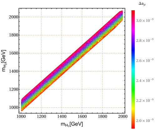
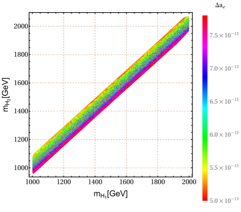
Figure 3: Correlation between the masses of the scalars $H_{1}$ and $H_{2}$ consistent with the muon and electron anomalous magnetic moments.

V Meson oscillations

In this section, we analyze the consequences of our proposed theory in the $K^{0}-\bar{K}^{0}$, $B_{d}^{0}-\bar{B}_{d}^{0}$ and $B_{s}^{0}-\bar{B}_{s}^{0}$ meson oscillations. These meson oscillations are caused by flavour violating down type quark interactions mediated by the tree level exchange of electrically neutral CP even and CP odd scalars as well as by the tree level $Z^{\prime}$ exchange. The $K^{0}-\bar{K}^{0}$, $B_{d}^{0}-\bar{B}_{d}^{0}$ and $B_{s}^{0}-\bar{B}_{s}^{0}$ meson oscillations are described by the following effective Hamiltonians:

$$\mathcal{H}_{eff}^{\left(K\right)}\mathcal{=}\sum_{j=1}^{3}c_{j}^{\left(K\right)}\left(\mu\right)\mathcal{O}_{j}^{\left(K\right)}\left(\mu\right)+\frac{g_{X}^{2}}{9m_{Z^{\prime}}^{2}}\left|\left(V_{DL}^{\ast}\right)_{32}\left(V_{DL}\right)_{31}\right|^{2}\mathcal{O}_{4}^{\left(K\right)},$$ (65)

$$\mathcal{H}_{eff}^{\left(B_{d}\right)}\mathcal{=}\sum_{j=1}^{3}c_{j}^{\left(B_{d}\right)}\left(\mu\right)\mathcal{O}_{j}^{\left(B_{d}\right)}\left(\mu\right)+\frac{g_{X}^{2}}{9m_{Z^{\prime}}^{2}}\left|\left(V_{DL}^{\ast}\right)_{31}\left(V_{DL}\right)_{33}\right|^{2}\mathcal{O}_{4}^{\left(B_{d}\right)},$$ (66)

$$\mathcal{H}_{eff}^{\left(B_{s}\right)}\mathcal{=}\sum_{j=1}^{3}c_{j}^{\left(B_{s}\right)}\left(\mu\right)\mathcal{O}_{j}^{\left(B_{s}\right)}\left(\mu\right)+\frac{g_{X}^{2}}{9m_{Z^{\prime}}^{2}}\left|\left(V_{DL}^{\ast}\right)_{32}\left(V_{DL}\right)_{33}\right|^{2}\mathcal{O}_{4}^{\left(B_{s}\right)},$$ (67)

where the operators relevant for the $K^{0}-\bar{K}^{0}$, $B_{d}^{0}-\bar{B}_{d}^{0}$ and $B_{s}^{0}-\bar{B}_{s}^{0}$ meson mixings have the form:

$$\mathcal{O}_{1}^{\left(K\right)} = \left(\overline{s}_{R}d_{L}\right)\left(\overline{s}_{R}d_{L}\right),\hskip 19.91684pt\hskip 19.91684pt\mathcal{O}_{2}^{\left(K\right)}=\left(\overline{s}_{L}d_{R}\right)\left(\overline{s}_{L}d_{R}\right),\hskip 19.91684pt$$ (68)

$$\mathcal{O}_{3}^{\left(K\right)} = \left(\overline{s}_{R}d_{L}\right)\left(\overline{s}_{L}d_{R}\right),\hskip 19.91684pt\hskip 19.91684pt\mathcal{O}_{4}^{\left(K\right)}=\left(\overline{s}_{L}\gamma_{\mu}d_{L}\right)\left(\overline{s}_{L}\gamma^{\mu}d_{L}\right),$$ (69)

$$\mathcal{O}_{1}^{\left(B_{d}\right)} = \left(\overline{d}_{R}b_{L}\right)\left(\overline{d}_{R}b_{L}\right),\hskip 19.91684pt\hskip 19.91684pt\mathcal{O}_{2}^{\left(B_{d}\right)}=\left(\overline{d}_{L}b_{R}\right)\left(\overline{d}_{L}b_{R}\right),\hskip 19.91684pt$$ (70)

$$\mathcal{O}_{3}^{\left(B_{d}\right)} = \left(\overline{d}_{R}b_{L}\right)\left(\overline{d}_{L}b_{R}\right),\hskip 19.91684pt\hskip 19.91684pt\mathcal{O}_{4}^{\left(B_{d}\right)}=\left(\overline{d}_{L}\gamma_{\mu}b_{L}\right)\left(\overline{d}_{L}\gamma^{\mu}b_{L}\right),$$ (71)

$$\mathcal{O}_{1}^{\left(B_{s}\right)} = \left(\overline{s}_{R}b_{L}\right)\left(\overline{s}_{R}b_{L}\right),\hskip 19.91684pt\hskip 19.91684pt\mathcal{O}_{2}^{\left(B_{s}\right)}=\left(\overline{s}_{L}b_{R}\right)\left(\overline{s}_{L}b_{R}\right),$$ (72)

$$\mathcal{O}_{3}^{\left(B_{s}\right)} = \left(\overline{s}_{R}b_{L}\right)\left(\overline{s}_{L}b_{R}\right),\hskip 19.91684pt\hskip 19.91684pt\mathcal{O}_{4}^{\left(B_{s}\right)}=\left(\overline{s}_{L}\gamma_{\mu}b_{L}\right)\left(\overline{s}_{L}\gamma^{\mu}b_{L}\right),$$ (73)

and the Wilson coefficients are:

$$c_{1}^{\left(K\right)} = \frac{z_{h\overline{s}_{R}d_{L}}^{2}}{m_{h}^{2}}+\sum_{j=1}^{2}\frac{z_{H_{j}\overline{s}_{R}d_{L}}^{2}}{M_{H_{j}}^{2}}-\sum_{j=1}^{2}\frac{z_{A_{j}\overline{s}_{R}d_{L}}^{2}}{M_{A_{j}}^{2}},$$ (74)

$$c_{2}^{\left(K\right)} = \frac{z_{h\overline{s}_{L}d_{R}}^{2}}{m_{h}^{2}}+\sum_{j=1}^{2}\frac{z_{H_{j}\overline{s}_{L}d_{R}}^{2}}{M_{H_{j}}^{2}}-\sum_{j=1}^{2}\frac{z_{A_{j}\overline{s}_{L}d_{R}}^{2}}{M_{A_{j}}^{2}},\hskip 19.91684pt\hskip 19.91684pt$$ (75)

$$c_{3}^{\left(K\right)} = \frac{z_{h\overline{s}_{R}d_{L}}z_{h\overline{s}_{L}d_{R}}}{m_{h}^{2}}+\sum_{j=1}^{2}\frac{z_{H_{j}\overline{s}_{R}d_{L}}z_{H_{j}\overline{s}_{L}d_{R}}}{M_{H_{j}}^{2}}-\sum_{j=1}^{2}\frac{z_{A_{j}\overline{s}_{R}d_{L}}z_{A_{j}\overline{s}_{L}d_{R}}}{M_{A_{j}}^{2}},$$ (76)

$$c_{1}^{\left(B_{d}\right)} = \frac{z_{h\overline{d}_{R}b_{L}}^{2}}{m_{h}^{2}}+\sum_{j=1}^{2}\frac{z_{H_{j}\overline{d}_{R}b_{L}}^{2}}{M_{H_{j}}^{2}}-\sum_{j=1}^{2}\frac{z_{A_{j}\overline{d}_{R}b_{L}}^{2}}{M_{A_{j}}^{2}},$$ (77)

$$c_{2}^{\left(B_{d}\right)} = \frac{z_{h\overline{d}_{L}b_{R}}^{2}}{m_{h}^{2}}+\sum_{j=1}^{2}\frac{z_{H_{j}\overline{d}_{L}b_{R}}^{2}}{M_{H_{j}}^{2}}-\sum_{j=1}^{2}\frac{z_{A_{j}\overline{d}_{L}b_{R}}^{2}}{M_{A_{j}}^{2}},$$ (78)

$$c_{3}^{\left(B_{d}\right)} = \frac{z_{h\overline{d}_{R}b_{L}}z_{h\overline{d}_{L}b_{R}}}{m_{h}^{2}}+\sum_{j=1}^{2}\frac{z_{H_{j}\overline{d}_{R}b_{L}}z_{H_{j}\overline{d}_{L}b_{R}}}{M_{H_{j}}^{2}}-\sum_{j=1}^{2}\frac{z_{A_{j}\overline{d}_{R}b_{L}}z_{A_{j}\overline{d}_{L}b_{R}}}{M_{A_{j}}^{2}},$$ (79)

$$c_{1}^{\left(B_{s}\right)} = \frac{z_{h\overline{s}_{R}b_{L}}^{2}}{m_{h}^{2}}+\sum_{j=1}^{2}\frac{z_{H_{j}\overline{s}_{R}b_{L}}^{2}}{M_{H_{i}}^{2}}-\sum_{j=1}^{2}\frac{z_{A_{j}\overline{s}_{R}b_{L}}^{2}}{M_{A_{j}}^{2}},$$ (80)

$$c_{2}^{\left(B_{s}\right)} = \frac{z_{h\overline{s}_{L}b_{R}}^{2}}{m_{h}^{2}}+\sum_{j=1}^{2}\frac{z_{H_{j}\overline{s}_{L}b_{R}}^{2}}{M_{H_{j}}^{2}}-\sum_{j=1}^{2}\frac{z_{A_{j}\overline{s}_{L}b_{R}}^{2}}{M_{A_{j}}^{2}},$$ (81)

$$c_{3}^{\left(B_{s}\right)} = \frac{z_{h\overline{s}_{R}b_{L}}z_{h\overline{s}_{L}b_{R}}}{m_{h}^{2}}+\sum_{j=1}^{2}\frac{z_{H_{j}\overline{s}_{R}b_{L}}z_{H_{j}\overline{s}_{L}b_{R}}}{M_{H_{j}}^{2}}-\sum_{j=1}^{2}\frac{z_{A_{j}\overline{s}_{R}b_{L}}z_{A_{j}\overline{s}_{L}b_{R}}}{M_{A_{j}}^{2}},$$ (82)

Furthermore, the following relations have been taken into account:

$$\widetilde{M}_{f} = \left(M_{f}\right)_{diag}=V_{fL}^{\dagger}M_{f}V_{fR},\hskip 28.45274pt\hskip 28.45274ptf_{\left(L,R\right)}=V_{f\left(L,R\right)}\widetilde{f}_{\left(L,R\right)},$$

$$\overline{f}_{iL}\left(M_{f}\right)_{ij}f_{jR} = \overline{\widetilde{f}}_{kL}\left(V_{fL}^{\dagger}\right)_{ki}\left(M_{f}\right)_{ij}\left(V_{fR}\right)_{jl}\widetilde{f}_{lR}=\overline{\widetilde{f}}_{kL}\left(V_{fL}^{\dagger}M_{f}V_{fR}\right)_{kl}\widetilde{f}_{lR}=\overline{\widetilde{f}}_{kL}\left(\widetilde{M}_{f}\right)_{kl}\widetilde{f}_{lR}=m_{fk}\overline{\widetilde{f}}_{kL}\widetilde{f}_{kR},$$

$$k = 1,2,3\,.$$ (83)

Here, $\widetilde{f}_{k\left(L,R\right)}$ and $f_{k\left(L,R\right)}$ ($k=1,2,3$) are the SM fermionic fields in the mass and interaction bases, respectively.

On the other hand, the $K-\bar{K}$, $B_{d}^{0}-\bar{B}_{d}^{0}$ and $B_{s}^{0}-\bar{B}_{s}^{0}$ meson mass differences are given by:

$$\Delta m_{K}=\Delta m_{K}^{\left(SM\right)}+\Delta m_{K}^{\left(NP\right)},\hskip 28.45274pt\Delta m_{B_{d}}=\Delta m_{B_{d}}^{\left(SM\right)}+\Delta m_{B_{d}}^{\left(NP\right)},\hskip 28.45274pt\Delta m_{B_{s}}=\Delta m_{B_{s}}^{\left(SM\right)}+\Delta m_{B_{s}}^{\left(NP\right)},$$ (84)

where $\Delta m_{K}^{\left(SM\right)}$, $\Delta m_{B_{d}}^{\left(SM\right)}$ and $\Delta m_{B_{s}}^{\left(SM\right)}$ stand for the SM contributions, while $\Delta m_{K}^{\left(NP\right)}$, $\Delta m_{B_{d}}^{\left(NP\right)}$ and $\Delta m_{B_{s}}^{\left(NP\right)}$ arise from new physics effects.

In the model under consideration, we find the following new physics contributions to the $K-\bar{K}$, $B_{d}^{0}-\bar{B}_{d}^{0}$ and $B_{s}^{0}-\bar{B}_{s}^{0}$ meson mass splittings:

$$\Delta m_{K}^{\left(NP\right)}=\frac{g_{X}^{2}}{9m_{Z^{\prime}}^{2}}\left|\left(V_{DL}^{\ast}\right)_{32}\left(V_{DL}\right)_{31}\right|^{2}f_{K}^{2}B_{K}\eta_{K}m_{K}+\frac{8}{3}f_{K}^{2}\eta_{K}B_{K}m_{K}\left[k_{2}^{\left(K\right)}c_{3}^{\left(K\right)}+k_{1}^{\left(K\right)}\left(c_{1}^{\left(K\right)}+c_{2}^{\left(K\right)}\right)\right]$$ (85)

$$\Delta m_{B_{d}}^{\left(NP\right)}=\frac{g_{X}^{2}}{9m_{Z^{\prime}}^{2}}\left|\left(V_{DL}^{\ast}\right)_{31}\left(V_{DL}\right)_{33}\right|^{2}f_{B_{d}}^{2}B_{B_{d}}\eta_{B_{d}}m_{B_{d}}+\frac{8}{3}f_{B_{d}}^{2}\eta_{B_{d}}B_{B_{d}}m_{B_{d}}\left[k_{2}^{\left(B_{d}\right)}c_{3}^{\left(B_{d}\right)}+k_{1}^{\left(B_{d}\right)}\left(c_{1}^{\left(B_{d}\right)}+c_{2}^{\left(B_{d}\right)}\right)\right]$$ (86)

$$\Delta m_{B_{s}}^{\left(NP\right)}=\frac{g_{X}^{2}}{9m_{Z^{\prime}}^{2}}\left|\left(V_{DL}^{\ast}\right)_{32}\left(V_{DL}\right)_{33}\right|^{2}f_{B_{s}}^{2}B_{B_{s}}\eta_{B_{s}}m_{B_{s}}+\frac{8}{3}f_{B_{s}}^{2}\eta_{B_{s}}B_{B_{s}}m_{B_{s}}\left[k_{2}^{\left(B_{s}\right)}c_{3}^{\left(B_{s}\right)}+k_{1}^{\left(B_{s}\right)}\left(c_{1}^{\left(B_{s}\right)}+c_{2}^{\left(B_{s}\right)}\right)\right]$$ (87)

In our numerical analysis, we use the following numerical values of the meson parameters Dedes:2002er ; Aranda:2012bv ; Khalil:2013ixa ; Queiroz:2016gif ; Buras:2016dxz ; Ferreira:2017tvy ; Duy:2020hhk :

$$\Delta m_{K} = \left(3.484\pm 0.006\right)\times 10^{-12}MeV,\hskip 42.67912pt\Delta m_{K}^{\left(SM\right)}=3.483\times 10^{-12}MeV$$

$$f_{K} = 160MeV,\hskip 42.67912ptB_{K}=0.85,\hskip 42.67912pt\eta_{K}=0.57,$$

$$k_{1}^{\left(K\right)} = -9.3,\hskip 42.67912ptk_{2}^{\left(K\right)}=30.6,\hskip 42.67912ptm_{K}=497.614MeV,\hskip 42.67912pt$$ (88)

$$\left(\Delta m_{B_{d}}\right)_{\exp} = \left(3.337\pm 0.033\right)\times 10^{-10}MeV,\hskip 42.67912pt\Delta m_{B_{d}}^{\left(SM\right)}=3.582\times 10^{-10}MeV,$$

$$f_{B_{d}} = 188MeV,\hskip 42.67912ptB_{B_{d}}=1.26,\hskip 42.67912pt\eta_{B_{d}}=0.55,$$

$$k_{1}^{\left(B_{d}\right)} = -0.52,\hskip 42.67912ptk_{2}^{\left(B_{d}\right)}=0.88,\hskip 42.67912ptm_{B_{d}}=5279.5MeV,\hskip 42.67912pt$$ (89)

$$\left(\Delta m_{B_{s}}\right)_{\exp} = \left(104.19\pm 0.8\right)\times 10^{-10}MeV,\hskip 42.67912pt\Delta m_{B_{s}}^{\left(SM\right)}=121.103\times 10^{-10}MeV,$$

$$f_{B_{s}} = 225MeV,\hskip 42.67912ptB_{B_{s}}=1.26,\hskip 42.67912pt\eta_{B_{s}}=0.55,$$

$$k_{1}^{\left(B_{s}\right)} = -0.52,\hskip 42.67912ptk_{2}^{\left(B_{s}\right)}=0.88,\hskip 42.67912ptm_{B_{s}}=5366.3MeV,\hskip 42.67912pt$$ (90)

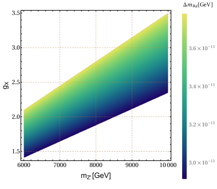
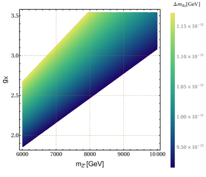
Figure 4: Allowed region in the $m_{Z^{\prime}}-g_{X}$ plane consistent with the constraint arising from $B_{d}^{0}-\bar{B}_{d}^{0}$ (left-plot) and $B_{s}^{0}-\bar{B}_{s}^{0}$ (right-plot) mixings. Here we fix the couplings of the flavor violating neutral Yukawa interactions as $2\times 10^{-4}$ and $10^{-3}$ for the left and right plots, respectively.

We plot in Figure 4 the allowed region in the $m_{Z^{\prime}}-g_{X}$ plane, consistent with the constraint arising from $B_{d}^{0}-\bar{B}_{d}^{0}$ (left-plot) and $B_{s}^{0}-\bar{B}_{s}^{0}$ (right-plot) mixings. In our numerical analysis we have considered a simplified benchmark scenario where the couplings of the flavor violating neutral Yukawa interactions responsible for the $B_{d}^{0}-\bar{B}_{d}^{0}$ and $B_{s}^{0}-\bar{B}_{s}^{0}$ mixings take values of about $2\times 10^{-4}$ and $10^{-3}$, respectively. Furthermore, we have set $M_{H_{1}}=1.2$ TeV, $M_{H_{2}}=1.3$ TeV, $M_{A_{1}}=M_{A_{2}}=1$ TeV and the $Z^{\prime}$ mass has been taken to be in the range $6$ TeV$\leqslant m_{Z^{\prime}}\leqslant$ $10$ TeV. As seen from Figure 4, the $B_{d}^{0}-\bar{B}_{d}^{0}$ and $B_{s}^{0}-\bar{B}_{s}^{0}$ meson oscillations caused by the flavor changing neutral interactions reach values close to their experimental upper limits, thus giving rise to the allowed regions in the $g_{X}-m_{Z^{\prime}}$ plane consistent with these constraints. On the other hand, concerning the $K^{0}-\bar{K}^{0}$ mixing, we have numerically checked that in the aforementioned simplified benchmark scenario and above-described region of parameter space with a corresponding flavor violating Yukawa coupling of the order of $0.5\times 10^{-5}$, the obtained values for the $\Delta m_{K}$ are consistent with the meson oscillation experimental data. It is worth mentioning that in our numerical analysis we have considered the case of real down quark Yukawa couplings, which implies that CP violation in the quark sector only arises from the up-type quark sector. Therefore, the constraints that are usually imposed on any possible new contributions to the $K^{0}-\bar{K}^{0}$, $B_{d}^{0}-\bar{B}_{d}^{0}$ and $B_{s}^{0}-\bar{B}_{s}^{0}$ meson oscillations, arising from CP-violating processes, are not relevant for our case.

VI Dark matter

Both the $SU(2)_{L}\times U(1)_{Y}\times U(1)_{X}$ gauge symmetry and the $Z_{4}$ discrete symmetry are spontaneously broken, whereas the $Z_{2}$ symmetry is preserved. This $Z_{2}$ conservation implies that the particles carrying a non trivial $Z_{2}$ charge always couple in pairs, and therefore the lightest of the electrically neutral $Z_{2}$ odd particles is a dark matter candidate. The considered model contains two kinds of candidates: the fermion singlet $\Psi_{nR}$ and the scalar singlets that are either $\varphi_{1}$ or $\varphi_{2}$. The fields, $\varphi_{1},\Psi_{nR}$, carry the X charge but the $\varphi_{2}$ does not. Except for the Yukawa interaction of $\varphi_{2}$ with new fermions $\Omega_{mR},\Psi_{nR}$, the $\varphi_{2}$ has only quartic scalar interactions. Thus, the $\varphi_{2}$ mainly annihilates into $W^{+}W^{-},ZZ,t\bar{t},b\bar{b},HH$ via a scalar portal interaction, and the relic density is governed by Higgs portal interactions and takes the form HuongRelic1

$$\Omega h^{2}\simeq 0.1\left(\frac{m_{\varphi_{2}}}{\lambda_{eff}\times 1.354\text{TeV}}\right)^{2},$$ (91)

where $\lambda_{eff}$ is an effective coupling, which depends on all trilinear Higgs couplings of $\varphi_{2}$ with the remaining Higgs. In order to consistently reproduce the experimental value of the dark matter relic density HuongRelic2 , $\Omega h^{2}=0.1198\pm 0.0026$, the mass $m_{\varphi_{2}}$ has to fulfill the constraint, $m_{\varphi_{2}}<\lambda_{eff}\times 1.5\text{TeV}$. If the effective coupling is in the range $0.5<\lambda_{eff}<1.5$, the dark matter mass satisfies $0.75\text{TeV}<m_{\varphi_{2}}<2.25\text{TeV}$. Since $\varphi_{2}$ is a gauge singlet scalar, it is electrically neutral, and then it only scatters off in a quark antiquark pair via SM Higgs portal interaction, which has a rate proportional to the quartic coupling of $\varphi_{2}^{2}H^{2}$, denoted as $\lambda_{D}$. The tree-level SM Higgs exchange produces a spin-independent cross section given by Directsearch :

$$\sigma_{\varphi_{2}-p,n}\simeq 3.88\times 10^{-45}\left(\frac{\lambda_{D}}{0.5}\right)^{2}\left(\frac{2\text{TeV}}{m_{\varphi_{2}}}\right)^{2}\text{cm}^{2}.$$ (92)

This scattering cross-section reaches the direct detection limit from the XENON1T experiment XENON1T for dark matter mass around $2\text{TeV}$ and effective coupling $\lambda_{D}\simeq 0.5.$ Unlike $\varphi_{2}$, $\varphi_{1}$ carries a $\text{X}-$charge. Thus, if $\varphi_{1}$ is a dark matter candidate, it will scatter off a nucleon not only through the exchange of the Higgs, but also via the exchange of a new neutral gauge boson. This obeys direct detection limits from the XENON1T experiment XENON1T , and yields the correct relic density if the dark matter mass is heavier than $3\text{TeV}$, (see in Queiroz ).
    Let us now assume that the dark matter is the neutral fermion, denoted $\Psi$. This is a $SU(2)_{L}$ singlet which does not carry hypercharge, but carries a $U(1)_{X}$ charge. Thus, the interaction of two dark matter candidates $\Psi$ with a new neutral gauge boson, called $Z_{X}$, determines the dark matter phenomenology. $\Psi_{n}$ annihilates into SM particles through the exchange of a new gauge boson. The relic density is given as Huong2019vej

$$\Omega_{\Phi}h^{2}\simeq 0.1\text{pb}\left(\frac{\alpha}{150\text{GeV}}\right)^{-2}\left(\frac{m_{\Psi}}{2.86\text{TeV}}\right)^{2},$$ (93)

where $\left(\frac{\alpha}{150\text{GeV}}\right)^{2}\simeq 1\text{pb}$. This relic density satisfies the experimental value HuongRelic2 if and only if $m_{\Psi}>3.13\text{TeV}$. At the tree-level, the dark matter $\Psi_{N}$ scatters off nuclei via the exchange of the gauge boson $\text{Z}_{X}$. In the limit, $m_{\Psi}>3.13\text{TeV}$, the cross-section of this scattering is predicted to be consistent with the XENON1T experiment (see Abada:2021yot ; HuongRelic1 ; Queiroz ).

VII Leptogenesis

Before counting flavored $\text{CP}-$asymmetry parameters from the decay of each heavy pseudo-Dirac neutrinos, we must rotate the sterile neutrinos $\nu_{aR},N_{aR}$, into their mass basis. As previously mentioned, the sterile neutrinos form three pairs of quasi-degenerate pseudo-Dirac fermions due to the small $\mu-$parameter, which is generated at two loop level. The eigenstates $\left(N_{aR}^{+},N_{aR}^{-}\right)$, corresponding to the eigenvalues $\left(M_{\nu}^{+},-M_{\nu}^{-}\right)$, are related to $\left(\nu_{Ra},N_{Ra}\right)$ through:

$$N_{aR}^{+}=\frac{1}{\sqrt{2}}\left(\nu_{aR}+N_{aR}\right),\hskip 8.5359pt\hskip 8.5359ptN_{aR}^{-}=\frac{i}{\sqrt{2}}\left(\nu_{aR}-N_{aR}\right).$$ (94)

Henceforth, the Yukawa interactions of $\nu_{aR},N_{aR}$ can be modified and written on the new basis as follows

$$-\mathcal{L}_{Y}^{l}\ni\sum_{i=1}^{3}\sum_{a=1}^{3}y_{ia}^{\nu}\overline{l}_{iL}\widetilde{\phi}_{2}\frac{\left(N_{aR}^{+}-iN_{aR}^{-}\right)}{\sqrt{2}}+\sum_{a=1}^{3}\sum_{n=1}^{2}\left(x_{N}\right)_{aj}\frac{\left(\overline{N^{+}}_{aR}+i\overline{N^{-}}_{aR}\right)}{\sqrt{2}}\Psi_{nR}^{C}\varphi_{1}$$ (95)

The lepton asymmetry is generated from the decay of the lightest pair of pseudo-Dirac neutrinos, called $(N_{\pm})$, and it can be enhanced due to a resonance effect Lepto1 ; Lepto2 ; Dib:2019jod . If $(N_{\pm})$ couples only with a SM lepton, the washout factor is determined from the inverse decay of the SM lepton and Higgs into the pair of pseudo-Dirac neutrinos. Since the washout factor has a quadratic suppression with the $\mu-$parameter Lepto3 ; Lepto4 , the smallness of $\mu$ can naturally suppress the washout factor. However, in our model, the $\mu-$parameter can be small in a technically natural way since it is generated at the two-loop level. Therefore, in addition to the inverse decay $lH^{\pm}\rightarrow N_{\pm}\rightarrow lH^{{}^{\pm}}$, the model creates new washout processes: $lH^{{}^{\pm}}\rightarrow N_{\pm}\rightarrow\Psi_{R}\varphi_{1}$ (see Eq.(95)). In the high-temperature region (temperature larger than the inverse see-saw scale), new washout processes can be avoided if the Yukawa couplings $(x_{aj}^{N})$ are very suppressed. This is unreasonable, because the $\mu-$parameter is generated at two loop level, as shown in Eq.(56). If the temperature of the Universe drops below the see-saw scale, the inverse decays producing $N_{aR}$ fall out of thermal equilibrium, and thermal leptogenesis can happen. Assuming that the fermions $\Psi_{nR}$ are heavier than the lightest pseudo-Dirac pair, $(N^{\pm})$, the lepton asymmetry generates via the decay of the lightest pair of pseudo-Dirac $(N_{\pm}\equiv N_{1}^{\pm})$ to the SM Higgs and lepton doublets and has the following form

$$\epsilon_{\pm}=\sum_{\alpha=1}^{3}\frac{\left\{\Gamma\left(N_{\pm}\rightarrow l_{\alpha}H^{+}\right)-\Gamma\left(N_{\pm}\rightarrow\bar{l}_{\alpha}H^{-}\right)\right\}}{\left\{\Gamma\left(N_{\pm}\rightarrow l_{\alpha}H^{+}\right)+\Gamma\left(N_{\pm}\rightarrow\bar{l}_{\alpha}H^{-}\right)\right\}}\simeq\frac{\mathop{\mathrm{I}m}\left\{\left(\left[\left(y_{N_{+}}\right)^{\dagger}\left(y_{N_{-}}\right)\right]^{2}\right)_{11}\right\}}{8\pi A_{\pm}}\frac{r}{r^{2}+\frac{\Gamma_{\mp}^{2}}{m_{N_{\mp}}^{2}}},$$ (96)

where $y_{N_{\pm}}=\frac{y^{\left(\nu\right)}}{\sqrt{2}}\left(1\pm\frac{1}{4}M^{-1}\mu\right),$ $r\equiv\frac{m_{N_{+}}^{2}-m_{N_{-}}^{2}}{m_{N_{+}}m_{N_{-}}},\hskip 8.5359ptA_{\pm}=\left((y^{\nu})^{{\dagger}}y^{\nu}\right)_{11},\hskip 8.5359pt\Gamma_{\pm}\equiv\frac{A_{\pm}m_{N_{\pm}}}{8\pi}$. In the weak and strong washout region, the approximate baryon asymmetry is estimated as

$$\eta_{B} = \frac{\epsilon_{N_{\pm}}}{g_{\ast}}\hskip 8.5359pt\text{for}\hskip 8.5359ptK_{N_{\pm}}^{eff}\ll 1,$$

$$\eta_{B} = \frac{0.3\epsilon_{N_{\pm}}}{g_{\ast}K_{N_{\pm}}^{eff}(\ln K_{N_{\pm}}^{eff})^{0.6}}\hskip 8.5359pt\text{for}\hskip 8.5359ptK_{N_{\pm}}^{eff}\gg 1.$$ (97)

Here, $g_{\ast}\simeq 118$ is the number of relativistic degrees of freedom. In the leptogenesis epoch, the effective washout parameter is defined as

$$K_{N_{\pm}}^{eff}\simeq\left(\frac{\Gamma_{+}+\Gamma_{-}}{H}\right)\left(\frac{m_{N^{+}}-m_{N^{-}}}{\Gamma_{\pm}}\right)^{2}$$ (98)

where $\text{H}=\sqrt{\frac{4\pi^{3}g_{\ast}}{45}}\frac{T^{2}}{M_{Pl}}$ is the Hubble constant. For a successful leptogenesis and inverse see-saw mechanism, we have to choose the parameter space including four Yukawa couplings $y^{\nu},y^{N},x_{N},x_{\Psi}$, two VEVs $v_{2},v_{\sigma}$, and as well as the masses of $\Omega_{n},\Psi_{n},\Im[\varphi_{i}],\Re[\varphi_{i}]$. To study this result more quantitatively it is convenient to use the Casas-Ibarra parametrization Casas ; Das:2012ze of the Yukawa coupling $y^{\nu}$, as follows

$$y^{\nu}=\frac{v_{\sigma}}{v_{2}}\left(\text{U}_{\text{PMNS}}\text{M}_{\nu}^{\frac{1}{2}}\text{R}\mu^{-\frac{1}{2}}y^{N}\right).$$ (99)

In this parametrization, R is a complex orthogonal matrix that has the general form

$$R=\left(\begin{array}[]{ccc}c_{y}c_{z}&-s_{x}c_{z}s_{y}-c_{x}s_{z}&s_{x}s_{z}-c_{x}s_{y}c_{z}\\ c_{y}s_{z}&c_{x}c_{z}-s_{x}s_{y}s_{z}&-c_{z}s_{x}-c_{x}s_{y}s_{z}\\ s_{y}&s_{x}c_{y}&c_{x}c_{y}\end{array}\right),$$ (100)

where $c_{x}=\cos x,s_{x}=\sin x$ and so on, with $x,y,z\in C$. Here $\text{U}_{\text{PMNS}}$ is the Pontecorvo-Maki-Nakagawa-Sakata mixing matrix for the lepton sector, while $\text{M}_{\nu}=\text{Diag}(m_{\nu_{1}},m_{\nu_{2}},m_{\nu_{3}})$ is a diagonal light active neutrino mass matrix. The current best fit values for the light neutrino masses, mixing angles and the CP violation phase of $\text{U}_{\text{PMNS}}$ are given in deSalas:2020pgw . In order to reduce the number of free parameters, we need to take some assumptions. Therefore, we fix the three complex mixing angles $x=0,y=z=\Re[\theta]+i\Im[\theta]$. Notice that the values of the Yukawas $y_{ij}^{\nu}$ are sensitive to the $\Im[\theta]$ but not sensitive to $\Re[\theta]$. Additionally, we assume that $Y^{(N)}$ is a diagonal matrix and is fixed as $Y^{(N)}=\text{Diag}(\text{0.5},\text{0.9i},\text{1.8})$. Two VEVs are chosen as $v_{2}=24.6\text{GeV}$, $v_{\sigma}\simeq 5\times 10^{3}\text{GeV }$. These choices guarantee that the gauge interactions of $N_{1}^{\pm}$ decouple at the leptogenesis epoch Mohapatra ; SFKing . In the perturbative region, the Yukawa coupling given in $(\ref{yu1})$ has to satisfy the condition: $(y^{\nu})_{ij}^{2}<4\pi$. Thus, the large-value domain of $\Im[\theta]$ is inhibited, namely $-2<\Im[\theta]<2$. With the above choices, the mass of light neutrinos can approach the experimental limit deSalas:2020pgw when $\mu$ satisfies: $\mu\simeq 1\text{keV}.$
    Figs.(5) show the strong sensitivity of the washout parameter with respect to $\Im[\theta]$, especially in the region of small values of $\Im[\theta]$. The strong washout regime, $K_{eff}\gg 1$, corresponds to small values of $\Im[\theta]$ (left panel), while the weak washout regime, $K_{eff}\ll 1$ corresponds to large values of $\Im[\theta]$ (right panel). For fixed values of $\Im[\theta]$, the washout parameter oscillates over $\Re[\theta]$ (see Figs. (6)), and the amplitude of oscillation increases as the value of $\Im[\theta]$ decreases. The washout effect is not affected much by $\Re[\theta]$.

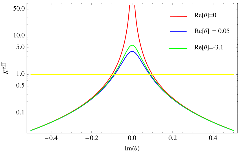
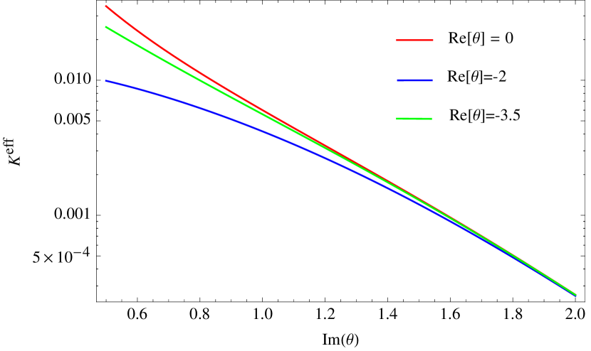
Figure 5: The washout parameter as a function of the $\Im[\theta]$.

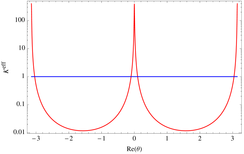
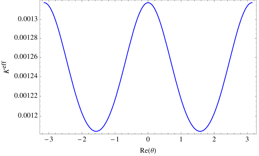
Figure 6: The washout parameter as a function of the $\Re[\theta]$. Left panel: $\Im[\theta]=0.005$, right panel: $\Im[\theta]=1.5$.

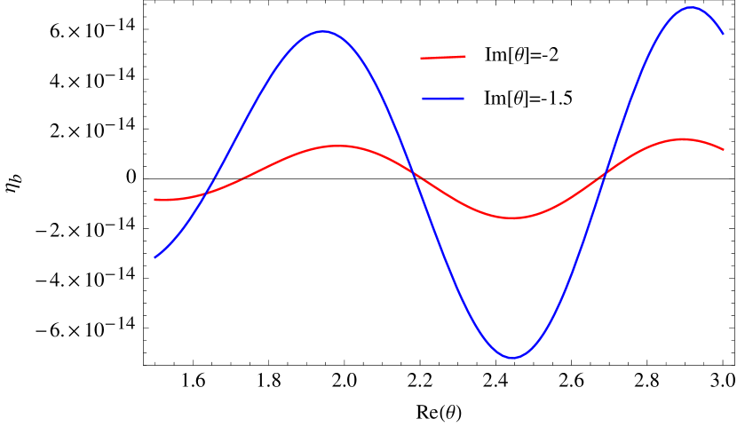
Figure 7: Estimating the baryon asymmetry in the weak-washout regime. Left panel:Log-Plot of the baryon asymmetry as a function of the $\Im[\theta]$. Right panel: Log-Plot the baryon asymmetry as a function of the $\Re[\theta]$.

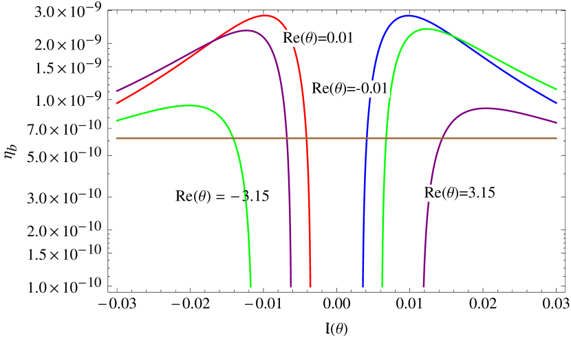
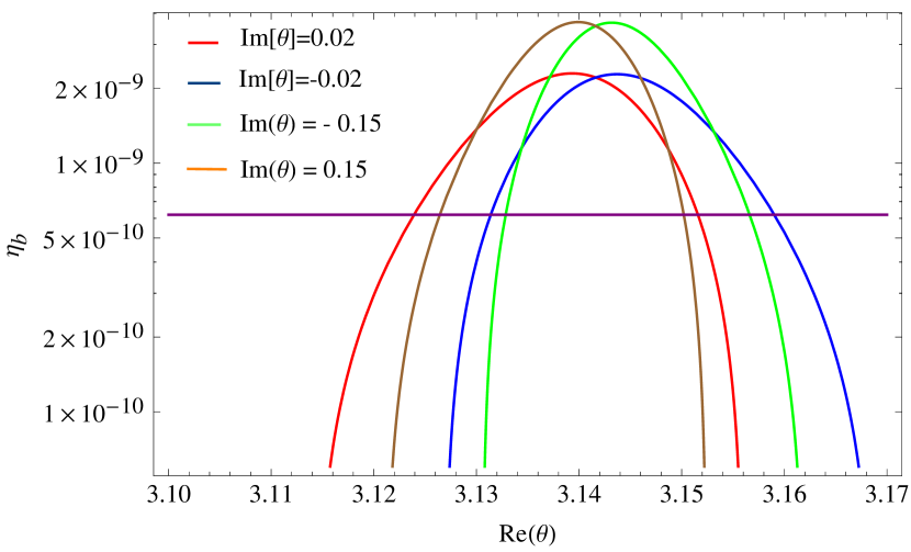
Figure 8: Estimating the baryon asymmetry in the strong-washout regime. Left panel: Plot of the baryon asymmetry as a function of the $\Im[\theta]$. Right panel: Plot of the baryon asymmetry as a function of the $\Re[\theta]$.

Figs. (7) show the generated baryon asymmetry from a numerical study of the approximate results of the Boltzmann equation, given in Eq.(97). In the weak washout regime, the predicted baryon asymmetry barely reaches the observed values $\eta_{B}\simeq 6.08\times 10^{-10}.$

In the strong-washout regime, the baryon asymmetry generation can reach the observed value, for the small phase entries of the R matrix. For small values of $\Im[\theta]$, we obtain the strong washout effect for every choice of $\Re[\theta]$ (see the left panel of Fig.(5)). However, not every value of $\Re[\theta]$ predicts a sufficient amount of baryon asymmetries for the Universe. The right-panel of Figs. (8) shows the amount of baryon asymmetry as a function of $\Re[\theta]$, which seems to drastically change under variations of $\Re[\theta]$. Fixing $\Re[\theta]$, the behavior of the baryon asymmetry as a function of the imaginary part of the complex angle $\theta$ appears in the left panel of Figs. (8). It drastically decreases as $\Im[\theta]$ increases. We conclude that in the present model leptogenesis is viable with a strong-washout regime if we include the small phase of the R matrix. The amount of baryon asymmetry oscillates according to $\theta$, and the oscillation amplitude can reach the observed value.

VIII Conclusions

We have built a 2HDM theory in which both particle content and symmetry are enlarged. We added several gauge singlet scalars and electrically charged vector-like fermions, as well as right-handed Majorana neutrinos, with the SM gauge symmetry being supplemented by a $U(1)_{X}\times Z_{2}\times Z_{4}$ family symmetry. We have built a renormalizable theory based on the given particle content, where to the best of our knowledge, for the first time an inverse seesaw mechanism produces the SM fermion mass hierarchy. The nonuniversal $U(1)_{X}$ gauge symmetry and the discrete $Z_{4}$ symmetry are spontaneously broken, whereas the $Z_{2}$ symmetry is preserved, thus allowing to have stable scalar and fermionic dark matter candidates. Our proposed theory is consistent with the observed SM fermion mass hierarchy, the tiny values for the light active neutrino masses, the lepton and baryon asymmetries of the Universe, the dark matter relic density, the meson oscillation experimental data as well as the muon and electron anomalous magnetic moments.

REFERENCES

- (1) A. Davidson and K. C. Wali, “Universal Seesaw Mechanism?,” Phys. Rev. Lett. 59 (1987) 393.
- (2) A. Davidson, S. Ranfone, and K. C. Wali, “Quark Masses and Mixing Angles From Universal Seesaw Mechanism,” Phys. Rev. D 41 (1990) 208.
- (3) A. Davidson and K. C. Wali, “Family Mass Hierarchy From Universal Seesaw Mechanism,” Phys. Rev. Lett. 60 (1988) 1813.
- (4) B. S. Balakrishna, A. L. Kagan, and R. N. Mohapatra, “Quark Mixings and Mass Hierarchy From Radiative Corrections,” Phys. Lett. B205 (1988) 345–352.
- (5) E. Ma, “Radiative Quark and Lepton Masses Through Soft Supersymmetry Breaking,” Phys. Rev. D39 (1989) 1922.
- (6) E. Ma, D. Ng, J. T. Pantaleone, and G.-G. Wong, “One Loop Induced Fermion Masses and Exotic Interactions in a Standard Model Context,” Phys. Rev. D40 (1989) 1586.
- (7) E. Ma, “Hierarchical Radiative Quark and Lepton Mass Matrices,” Phys. Rev. Lett. 64 (1990) 2866–2869.
- (8) E. Ma, “Pathways to naturally small neutrino masses,” Phys. Rev. Lett. 81 (1998) 1171–1174, arXiv:hep-ph/9805219 [hep-ph].
- (9) T. Kitabayashi and M. Yasue, “Radiatively induced neutrino masses and oscillations in an SU(3)(L) x U(1)(N) gauge model,” Phys. Rev. D63 (2001) 095002, arXiv:hep-ph/0010087 [hep-ph].
- (10) E. Ma, “Verifiable radiative seesaw mechanism of neutrino mass and dark matter,” Phys. Rev. D73 (2006) 077301, arXiv:hep-ph/0601225 [hep-ph].
- (11) P. V. Dong, D. T. Huong, T. T. Huong, and H. N. Long, “Fermion masses in the economical 3-3-1 model,” Phys. Rev. D74 (2006) 053003, arXiv:hep-ph/0607291 [hep-ph].
- (12) D. Chang and H. N. Long, “Interesting radiative patterns of neutrino mass in an SU(3)(C) x SU(3)(L) x U(1)(X) model with right-handed neutrinos,” Phys. Rev. D73 (2006) 053006, arXiv:hep-ph/0603098 [hep-ph].
- (13) P.-H. Gu and U. Sarkar, “Radiative Neutrino Mass, Dark Matter and Leptogenesis,” Phys. Rev. D77 (2008) 105031, arXiv:0712.2933 [hep-ph].
- (14) E. Ma and D. Suematsu, “Fermion Triplet Dark Matter and Radiative Neutrino Mass,” Mod. Phys. Lett. A24 (2009) 583–589, arXiv:0809.0942 [hep-ph].
- (15) D. Aristizabal Sierra, J. Kubo, D. Restrepo, D. Suematsu, and O. Zapata, “Radiative seesaw: Warm dark matter, collider and lepton flavour violating signals,” Phys. Rev. D79 (2009) 013011, arXiv:0808.3340 [hep-ph].
- (16) E. Nardi, D. Restrepo, and M. Velasquez, “Neutrino Masses in with Adjoint Flavons,” Eur. Phys. J. C72 (2012) 1941, arXiv:1108.0722 [hep-ph].
- (17) D. T. Huong, L. T. Hue, M. C. Rodriguez, and H. N. Long, “Supersymmetric reduced minimal 3-3-1 model,” Nucl. Phys. B870 (2013) 293–322, arXiv:1210.6776 [hep-ph].
- (18) D. Restrepo, O. Zapata, and C. E. Yaguna, “Models with radiative neutrino masses and viable dark matter candidates,” JHEP 11 (2013) 011, arXiv:1308.3655 [hep-ph].
- (19) E. Ma, I. Picek, and B. Radovčić, “New Scotogenic Model of Neutrino Mass with Gauge Interaction,” Phys. Lett. B726 (2013) 744–746, arXiv:1308.5313 [hep-ph].
- (20) E. Ma, “Radiative Origin of All Quark and Lepton Masses through Dark Matter with Flavor Symmetry,” Phys. Rev. Lett. 112 (2014) 091801, arXiv:1311.3213 [hep-ph].
- (21) A. E. Carcamo Hernandez, R. Martinez, and F. Ochoa, “Radiative seesaw-type mechanism of quark masses in ,” Phys. Rev. D87 no. 7, (2013) 075009, arXiv:1302.1757 [hep-ph].
- (22) A. E. Carcamo Hernandez, I. de Medeiros Varzielas, S. G. Kovalenko, H. Päs, and I. Schmidt, “Lepton masses and mixings in an multi-Higgs model with a radiative seesaw mechanism,” Phys. Rev. D88 no. 7, (2013) 076014, arXiv:1307.6499 [hep-ph].
- (23) H. Okada and K. Yagyu, “Radiative generation of lepton masses,” Phys. Rev. D89 no. 5, (2014) 053008, arXiv:1311.4360 [hep-ph].
- (24) D. Aristizabal Sierra, A. Degee, L. Dorame, and M. Hirsch, “Systematic classification of two-loop realizations of the Weinberg operator,” JHEP 03 (2015) 040, arXiv:1411.7038 [hep-ph].
- (25) M. D. Campos, A. E. Cárcamo Hernández, S. Kovalenko, I. Schmidt, and E. Schumacher, “Fermion masses and mixings in an grand unified model with an extra flavor symmetry,” Phys. Rev. D90 no. 1, (2014) 016006, arXiv:1403.2525 [hep-ph].
- (26) S. M. Boucenna, S. Morisi, and J. W. F. Valle, “Radiative neutrino mass in 3-3-1 scheme,” Phys. Rev. D90 no. 1, (2014) 013005, arXiv:1405.2332 [hep-ph].
- (27) A. E. Cárcamo Hernández, “A novel and economical explanation for SM fermion masses and mixings,” Eur. Phys. J. C76 no. 9, (2016) 503, arXiv:1512.09092 [hep-ph].
- (28) A. Aranda and E. Peinado, “A new radiative neutrino mass generation mechanism with higher dimensional scalar representations and custodial symmetry,” Phys. Lett. B754 (2016) 11–13, arXiv:1508.01200 [hep-ph].
- (29) D. Restrepo, A. Rivera, M. Sánchez-Peláez, O. Zapata, and W. Tangarife, “Radiative Neutrino Masses in the Singlet-Doublet Fermion Dark Matter Model with Scalar Singlets,” Phys. Rev. D92 no. 1, (2015) 013005, arXiv:1504.07892 [hep-ph].
- (30) R. Longas, D. Portillo, D. Restrepo, and O. Zapata, “The Inert Zee Model,” JHEP 03 (2016) 162, arXiv:1511.01873 [hep-ph].
- (31) S. Fraser, E. Ma, and M. Zakeri, “Verifiable Associated Processes from Radiative Lepton Masses with Dark Matter,” Phys. Rev. D93 no. 11, (2016) 115019, arXiv:1511.07458 [hep-ph].
- (32) S. Fraser, C. Kownacki, E. Ma, and O. Popov, “Type II Radiative Seesaw Model of Neutrino Mass with Dark Matter,” Phys. Rev. D93 no. 1, (2016) 013021, arXiv:1511.06375 [hep-ph].
- (33) H. Okada, N. Okada, and Y. Orikasa, “Radiative seesaw mechanism in a minimal 3-3-1 model,” Phys. Rev. D93 no. 7, (2016) 073006, arXiv:1504.01204 [hep-ph].
- (34) W. Wang and Z.-L. Han, “Radiative linear seesaw model, dark matter, and ,” Phys. Rev. D92 (2015) 095001, arXiv:1508.00706 [hep-ph].
- (35) D. Aristizabal Sierra, C. Simoes, and D. Wegman, “Closing in on minimal dark matter and radiative neutrino masses,” JHEP 06 (2016) 108, arXiv:1603.04723 [hep-ph].
- (36) C. Arbeláez, A. E. Cárcamo Hernández, S. Kovalenko, and I. Schmidt, “Radiative Seesaw-type Mechanism of Fermion Masses and Non-trivial Quark Mixing,” Eur. Phys. J. C77 no. 6, (2017) 422, arXiv:1602.03607 [hep-ph].
- (37) T. Nomura and H. Okada, “Radiatively induced Quark and Lepton Mass Model,” Phys. Lett. B761 (2016) 190–196, arXiv:1606.09055 [hep-ph].
- (38) T. Nomura and H. Okada, “Four-loop Neutrino Model Inspired by Diphoton Excess at 750 GeV,” Phys. Lett. B755 (2016) 306–311, arXiv:1601.00386 [hep-ph].
- (39) C. Kownacki and E. Ma, “Gauge dark symmetry and radiative light fermion masses,” Phys. Lett. B760 (2016) 59–62, arXiv:1604.01148 [hep-ph].
- (40) C. Kownacki, E. Ma, N. Pollard, and M. Zakeri, “Generalized Gauge U(1) Family Symmetry for Quarks and Leptons,” Phys. Lett. B766 (2017) 149–152, arXiv:1611.05017 [hep-ph].
- (41) T. Nomura, H. Okada, and N. Okada, “A Colored KNT Neutrino Model,” Phys. Lett. B762 (2016) 409–414, arXiv:1608.02694 [hep-ph].
- (42) J. E. Camargo-Molina, A. P. Morais, A. Ordell, R. Pasechnik, M. O. P. Sampaio, and J. Wessén, “Reviving trinification models through an E6 -extended supersymmetric GUT,” Phys. Rev. D95 no. 7, (2017) 075031, arXiv:1610.03642 [hep-ph].
- (43) J. E. Camargo-Molina, A. P. Morais, R. Pasechnik, and J. Wessén, “On a radiative origin of the Standard Model from Trinification,” JHEP 09 (2016) 129, arXiv:1606.03492 [hep-ph].
- (44) F. von der Pahlen, G. Palacio, D. Restrepo, and O. Zapata, “Radiative Type III Seesaw Model and its collider phenomenology,” Phys. Rev. D94 no. 3, (2016) 033005, arXiv:1605.01129 [hep-ph].
- (45) C. Bonilla, E. Ma, E. Peinado, and J. W. F. Valle, “Two-loop Dirac neutrino mass and WIMP dark matter,” Phys. Lett. B762 (2016) 214–218, arXiv:1607.03931 [hep-ph].
- (46) P.-H. Gu, “High-scale leptogenesis with three-loop neutrino mass generation and dark matter,” JHEP 04 (2017) 159, arXiv:1611.03256 [hep-ph].
- (47) A. Das, T. Nomura, H. Okada, and S. Roy, “Generation of a radiative neutrino mass in the linear seesaw framework, charged lepton flavor violation, and dark matter,” Phys. Rev. D 96 no. 7, (2017) 075001, arXiv:1704.02078 [hep-ph].
- (48) T. Nomura and H. Okada, “Loop induced type-II seesaw model and GeV dark matter with gauge symmetry,” Phys. Lett. B774 (2017) 575–581, arXiv:1704.08581 [hep-ph].
- (49) T. Nomura and H. Okada, “Radiative neutrino mass in an alternative gauge symmetry,” Nucl. Phys. B941 (2019) 586–599, arXiv:1705.08309 [hep-ph].
- (50) T. Nomura and H. Okada, “A model with isospin doublet gauge symmetry,” Int. J. Mod. Phys. A33 no. 14n15, (2018) 1850089, arXiv:1706.05268 [hep-ph].
- (51) W. Wang, R. Wang, Z.-L. Han, and J.-Z. Han, “The Scotogenic Models for Dirac Neutrino Masses,” Eur. Phys. J. C77 no. 12, (2017) 889, arXiv:1705.00414 [hep-ph].
- (52) N. Bernal, A. E. Cárcamo Hernández, I. de Medeiros Varzielas, and S. Kovalenko, “Fermion masses and mixings and dark matter constraints in a model with radiative seesaw mechanism,” JHEP 05 (2018) 053, arXiv:1712.02792 [hep-ph].
- (53) A. E. Cárcamo Hernández and H. N. Long, “A highly predictive flavour 3-3-1 model with radiative inverse seesaw mechanism,” J. Phys. G45 no. 4, (2018) 045001, arXiv:1705.05246 [hep-ph].
- (54) A. E. Cárcamo Hernández, S. Kovalenko, H. N. Long, and I. Schmidt, “A variant of 3-3-1 model for the generation of the SM fermion mass and mixing pattern,” JHEP 07 (2018) 144, arXiv:1705.09169 [hep-ph].
- (55) E. Ma and U. Sarkar, “Radiative Left-Right Dirac Neutrino Mass,” Phys. Lett. B776 (2018) 54–57, arXiv:1707.07698 [hep-ph].
- (56) R. Cepedello, M. Hirsch, and J. C. Helo, “Loop neutrino masses from operator,” JHEP 07 (2017) 079, arXiv:1705.01489 [hep-ph].
- (57) A. Dev and R. N. Mohapatra, “Natural Alignment of Quark Flavors and Radiatively Induced Quark Mixings,” Phys. Rev. D98 no. 7, (2018) 073002, arXiv:1804.01598 [hep-ph].
- (58) A. E. Cárcamo Hernández, S. Kovalenko, J. W. F. Valle, and C. A. Vaquera-Araujo, “Neutrino predictions from a left-right symmetric flavored extension of the standard model,” JHEP 02 (2019) 065, arXiv:1811.03018 [hep-ph].
- (59) N. Rojas, R. Srivastava, and J. W. F. Valle, “Simplest Scoto-Seesaw Mechanism,” Phys. Lett. B789 (2019) 132–136, arXiv:1807.11447 [hep-ph].
- (60) T. Nomura and H. Okada, “Zee-Babu type model with gauge symmetry,” Phys. Rev. D97 no. 9, (2018) 095023, arXiv:1803.04795 [hep-ph].
- (61) M. Reig, D. Restrepo, J. W. F. Valle, and O. Zapata, “Bound-state dark matter and Dirac neutrino masses,” Phys. Rev. D97 no. 11, (2018) 115032, arXiv:1803.08528 [hep-ph].
- (62) N. Bernal, D. Restrepo, C. Yaguna, and O. Zapata, “Two-component dark matter and a massless neutrino in a new model,” Phys. Rev. D99 no. 1, (2019) 015038, arXiv:1808.03352 [hep-ph].
- (63) J. Calle, D. Restrepo, C. E. Yaguna, and O. Zapata, “Minimal radiative Dirac neutrino mass models,” Phys. Rev. D99 no. 7, (2019) 075008, arXiv:1812.05523 [hep-ph].
- (64) A. Aranda, C. Bonilla, and E. Peinado, “Dynamical generation of neutrino mass scales,” Phys. Lett. B792 (2019) 40–42, arXiv:1808.07727 [hep-ph].
- (65) R. Cepedello, R. M. Fonseca, and M. Hirsch, “Systematic classification of three-loop realizations of the Weinberg operator,” JHEP 10 (2018) 197, arXiv:1807.00629 [hep-ph]. [erratum: JHEP06,034(2019)].
- (66) A. E. Cárcamo Hernández, J. Vignatti, and A. Zerwekh, “Generating lepton masses and mixings with a heavy vector doublet,” J. Phys. G46 no. 11, (2019) 115007, arXiv:1807.05321 [hep-ph].
- (67) E. Ma, “, Seesaw Dark Matter, and Higgs Decay,” arXiv:1810.06506 [hep-ph].
- (68) E. Ma, “ and Seesaw Dirac Neutrinos,” arXiv:1811.09645 [hep-ph].
- (69) S.-P. Li, X.-Q. Li, and Y.-D. Yang, “Muon in a -symmetric Two-Higgs-Doublet Model,” Phys. Rev. D 99 no. 3, (2019) 035010, arXiv:1808.02424 [hep-ph].
- (70) P. Arnan, A. Crivellin, M. Fedele, and F. Mescia, “Generic Loop Effects of New Scalars and Fermions in , and a Vector-like Generation,” JHEP 06 (2019) 118, arXiv:1904.05890 [hep-ph].
- (71) E. Ma, “Two-loop Dirac neutrino masses and mixing, with self-interacting dark matter,” Nucl. Phys. B946 (2019) 114725, arXiv:1907.04665 [hep-ph].
- (72) E. Ma, “Scotogenic cobimaximal Dirac neutrino mixing from and ,” Eur. Phys. J. C79 no. 11, (2019) 903, arXiv:1905.01535 [hep-ph].
- (73) A. E. Cárcamo Hernández, S. Kovalenko, R. Pasechnik, and I. Schmidt, “Phenomenology of an extended IDM with loop-generated fermion mass hierarchies,” Eur. Phys. J. C79 no. 7, (2019) 610, arXiv:1901.09552 [hep-ph].
- (74) E. Ma, “Scotogenic Dirac neutrinos,” Phys. Lett. B793 (2019) 411–414, arXiv:1901.09091 [hep-ph].
- (75) T. Nomura and H. Okada, “A two loop induced neutrino mass model with modular symmetry,” Nucl. Phys. B966 (2021) 115372, arXiv:1906.03927 [hep-ph].
- (76) T. Nomura and H. Okada, “A radiative neutrino mass model with hidden gauge symmetry inducing semi-annihilating dark matter,” arXiv:1904.13066 [hep-ph].
- (77) T. Nomura and H. Okada, “A modular symmetric model of dark matter and neutrino,” Phys. Lett. B797 (2019) 134799, arXiv:1904.03937 [hep-ph].
- (78) S. Centelles Chuliá, R. Cepedello, E. Peinado, and R. Srivastava, “Scotogenic dark symmetry as a residual subgroup of Standard Model symmetries,” Chin. Phys. C44 no. 8, (2020) 083110, arXiv:1901.06402 [hep-ph].
- (79) C. Bonilla, S. Centelles-Chuliá, R. Cepedello, E. Peinado, and R. Srivastava, “Dark matter stability and Dirac neutrinos using only Standard Model symmetries,” Phys. Rev. D101 no. 3, (2020) 033011, arXiv:1812.01599 [hep-ph].
- (80) S. Pramanick, “Scotogenic S3 symmetric generation of realistic neutrino mixing,” Phys. Rev. D100 no. 3, (2019) 035009, arXiv:1904.07558 [hep-ph].
- (81) C. Arbeláez, A. E. Cárcamo Hernández, R. Cepedello, M. Hirsch, and S. Kovalenko, “Radiative type-I seesaw neutrino masses,” Phys. Rev. D100 no. 11, (2019) 115021, arXiv:1910.04178 [hep-ph].
- (82) I. M. Ávila, V. De Romeri, L. Duarte, and J. W. F. Valle, “Phenomenology of scotogenic scalar dark matter,” Eur. Phys. J. C80 no. 10, (2020) 908, arXiv:1910.08422 [hep-ph].
- (83) A. E. Cárcamo Hernández, S. Kovalenko, R. Pasechnik, and I. Schmidt, “Sequentially loop-generated quark and lepton mass hierarchies in an extended Inert Higgs Doublet model,” JHEP 06 (2019) 056, arXiv:1901.02764 [hep-ph].
- (84) A. E. Cárcamo Hernández, D. T. Huong, and H. N. Long, “Minimal model for the fermion flavor structure, mass hierarchy, dark matter, leptogenesis, and the electron and muon anomalous magnetic moments,” Phys. Rev. D102 no. 5, (2020) 055002, arXiv:1910.12877 [hep-ph].
- (85) C. Arbeláez, A. E. Cárcamo Hernández, R. Cepedello, S. Kovalenko, and I. Schmidt, “Sequentially loop suppressed fermion masses from a single discrete symmetry,” JHEP 06 (2020) 043, arXiv:1911.02033 [hep-ph].
- (86) A. E. Cárcamo Hernández, L. T. Hue, S. Kovalenko, and H. N. Long, “An extended 3-3-1 model with two scalar triplets and linear seesaw mechanism,” arXiv:2001.01748 [hep-ph].
- (87) A. E. Cárcamo Hernández, C. O. Dib, and U. J. Saldaña-Salazar, “When meets all the mixing angles,” Phys. Lett. B809 (2020) 135750, arXiv:2001.07140 [hep-ph].
- (88) A. E. Cárcamo Hernández, Y. Hidalgo Velásquez, S. Kovalenko, H. N. Long, N. A. Pérez-Julve, and V. V. Vien, “Fermion spectrum and anomalies in a low scale 3-3-1 model,” Eur. Phys. J. C81 no. 2, (2021) 191, arXiv:2002.07347 [hep-ph].
- (89) A. E. Cárcamo Hernández, D. T. Huong, S. Kovalenko, A. P. Morais, R. Pasechnik, and I. Schmidt, “How low-scale trinification sheds light in the flavor hierarchies, neutrino puzzle, dark matter, and leptogenesis,” Phys. Rev. D102 no. 9, (2020) 095003, arXiv:2004.11450 [hep-ph].
- (90) A. E. Cárcamo Hernández, J. W. F. Valle, and C. A. Vaquera-Araujo, “Simple theory for scotogenic dark matter with residual matter-parity,” Phys. Lett. B809 (2020) 135757, arXiv:2006.06009 [hep-ph].
- (91) A. E. C. Hernández and I. Schmidt, “A renormalizable left-right symmetric model with low scale seesaw mechanisms,” arXiv:2101.02718 [hep-ph].
- (92) A. E. Cárcamo Hernández, C. Espinoza, J. Carlos Gómez-Izquierdo, and M. Mondragón, “Fermion masses and mixings, dark matter, leptogenesis and muon anomaly in an extended 2HDM with inverse seesaw,” arXiv:2104.02730 [hep-ph].
- (93) A. E. Cárcamo Hernández, S. Kovalenko, M. Maniatis, and I. Schmidt, “Fermion mass hierarchy and g-2 anomalies in an extended 3HDM Model,” arXiv:2104.07047 [hep-ph].
- (94) A. E. Cárcamo Hernández, S. Kovalenko, F. S. Queiroz, and Y. S. Villamizar, “An extended 3-3-1 model with radiative linear seesaw mechanism,” arXiv:2105.01731 [hep-ph].
- (95) A. Abada, N. Bernal, A. E. C. Hernández, X. Marcano, and G. Piazza, “Gauged inverse seesaw from dark matter,” Eur. Phys. J. C 81 no. 8, (2021) 758, arXiv:2107.02803 [hep-ph].
- (96) C. Bonilla, A. E. C. Hernández, J. a. Gonçalves, F. F. Freitas, A. P. Morais, and R. Pasechnik, “Collider signatures of vector-like fermions from a flavor symmetric 2HDM,” arXiv:2107.14165 [hep-ph].
- (97) A. E. C. Hernández, C. Hati, S. Kovalenko, J. W. F. Valle, and C. A. Vaquera-Araujo, “Scotogenic neutrino masses with gauged matter parity and gauge coupling unification,” arXiv:2109.05029 [hep-ph].
- (98) E. Kiritsis and P. Anastasopoulos, “The Anomalous magnetic moment of the muon in the D-brane realization of the standard model,” JHEP 05 (2002) 054, arXiv:hep-ph/0201295.
- (99) T. Appelquist, M. Piai, and R. Shrock, “Lepton dipole moments in extended technicolor models,” Phys. Lett. B593 (2004) 175–180, arXiv:hep-ph/0401114 [hep-ph].
- (100) G. F. Giudice, P. Paradisi, and M. Passera, “Testing new physics with the electron g-2,” JHEP 11 (2012) 113, arXiv:1208.6583 [hep-ph].
- (101) Y. Omura, E. Senaha, and K. Tobe, “Lepton-flavor-violating Higgs decay and muon anomalous magnetic moment in a general two Higgs doublet model,” JHEP 05 (2015) 028, arXiv:1502.07824 [hep-ph].
- (102) A. Falkowski, S. F. King, E. Perdomo, and M. Pierre, “Flavourful portal for vector-like neutrino Dark Matter and ,” JHEP 08 (2018) 061, arXiv:1803.04430 [hep-ph].
- (103) A. Crivellin, M. Hoferichter, and P. Schmidt-Wellenburg, “Combined explanations of and implications for a large muon EDM,” Phys. Rev. D98 no. 11, (2018) 113002, arXiv:1807.11484 [hep-ph].
- (104) B. Allanach, F. S. Queiroz, A. Strumia, and S. Sun, “ models for the LHCb and muon anomalies,” Phys. Rev. D93 no. 5, (2016) 055045, arXiv:1511.07447 [hep-ph]. [Erratum: Phys. Rev.D95,no.11,119902(2017)].
- (105) B. P. Padley, K. Sinha, and K. Wang, “Natural Supersymmetry, Muon , and the Last Crevices for the Top Squark,” Phys. Rev. D92 no. 5, (2015) 055025, arXiv:1505.05877 [hep-ph].
- (106) C.-H. Chen, T. Nomura, and H. Okada, “Explanation of and muon , and implications at the LHC,” Phys. Rev. D94 no. 11, (2016) 115005, arXiv:1607.04857 [hep-ph].
- (107) S. Raby and A. Trautner, “Vectorlike chiral fourth family to explain muon anomalies,” Phys. Rev. D97 no. 9, (2018) 095006, arXiv:1712.09360 [hep-ph].
- (108) C.-W. Chiang, H. Okada, and E. Senaha, “Dark matter, muon , electric dipole moments, and in a one-loop induced neutrino model,” Phys. Rev. D96 no. 1, (2017) 015002, arXiv:1703.09153 [hep-ph].
- (109) C.-H. Chen, T. Nomura, and H. Okada, “Excesses of muon , , and in a leptoquark model,” Phys. Lett. B774 (2017) 456–464, arXiv:1703.03251 [hep-ph].
- (110) E. Megias, M. Quiros, and L. Salas, “ from Vector-Like Leptons in Warped Space,” JHEP 05 (2017) 016, arXiv:1701.05072 [hep-ph].
- (111) H. Davoudiasl and W. J. Marciano, “Tale of two anomalies,” Phys. Rev. D98 no. 7, (2018) 075011, arXiv:1806.10252 [hep-ph].
- (112) J. Liu, C. E. M. Wagner, and X.-P. Wang, “A light complex scalar for the electron and muon anomalous magnetic moments,” JHEP 03 (2019) 008, arXiv:1810.11028 [hep-ph].
- (113) T. Nomura and H. Okada, “Muon anomalous magnetic moment, boson decays, and collider physics in multicharged particles,” Phys. Rev. D101 no. 1, (2020) 015021, arXiv:1903.05958 [hep-ph].
- (114) J. Kawamura, S. Raby, and A. Trautner, “Complete vectorlike fourth family and new for muon anomalies,” Phys. Rev. D100 no. 5, (2019) 055030, arXiv:1906.11297 [hep-ph].
- (115) M. Bauer, M. Neubert, S. Renner, M. Schnubel, and A. Thamm, “Axionlike Particles, Lepton-Flavor Violation, and a New Explanation of and ,” Phys. Rev. Lett. 124 no. 21, (2020) 211803, arXiv:1908.00008 [hep-ph].
- (116) F. J. Botella, F. Cornet-Gomez, and M. Nebot, “Flavor conservation in two-Higgs-doublet models,” Phys. Rev. D98 no. 3, (2018) 035046, arXiv:1803.08521 [hep-ph].
- (117) X.-F. Han, T. Li, L. Wang, and Y. Zhang, “Simple interpretations of lepton anomalies in the lepton-specific inert two-Higgs-doublet model,” Phys. Rev. D99 no. 9, (2019) 095034, arXiv:1812.02449 [hep-ph].
- (118) L. Wang, J. M. Yang, M. Zhang, and Y. Zhang, “Revisiting lepton-specific 2HDM in light of muon anomaly,” Phys. Lett. B788 (2019) 519–529, arXiv:1809.05857 [hep-ph].
- (119) B. Dutta and Y. Mimura, “Electron with flavor violation in MSSM,” Phys. Lett. B790 (2019) 563–567, arXiv:1811.10209 [hep-ph].
- (120) M. Badziak and K. Sakurai, “Explanation of electron and muon g - 2 anomalies in the MSSM,” JHEP 10 (2019) 024, arXiv:1908.03607 [hep-ph].
- (121) M. Endo and W. Yin, “Explaining electron and muon anomaly in SUSY without lepton-flavor mixings,” JHEP 08 (2019) 122, arXiv:1906.08768 [hep-ph].
- (122) G. Hiller, C. Hormigos-Feliu, D. F. Litim, and T. Steudtner, “Anomalous magnetic moments from asymptotic safety,” Phys. Rev. D102 no. 7, (2020) 071901, arXiv:1910.14062 [hep-ph].
- (123) A. E. Cárcamo Hernández, S. F. King, H. Lee, and S. J. Rowley, “Is it possible to explain the muon and electron in a model?,” Phys. Rev. D101 no. 11, (2020) 115016, arXiv:1910.10734 [hep-ph].
- (124) J. Kawamura, S. Raby, and A. Trautner, “Complete vectorlike fourth family with : A global analysis,” Phys. Rev. D101 no. 3, (2020) 035026, arXiv:1911.11075 [hep-ph].
- (125) D. Sabatta, A. S. Cornell, A. Goyal, M. Kumar, B. Mellado, and X. Ruan, “Connecting muon anomalous magnetic moment and multi-lepton anomalies at LHC,” Chin. Phys. C44 no. 6, (2020) 063103, arXiv:1909.03969 [hep-ph].
- (126) K.-F. Chen, C.-W. Chiang, and K. Yagyu, “An explanation for the muon and electron anomalies and dark matter,” JHEP 09 (2020) 119, arXiv:2006.07929 [hep-ph].
- (127) S. Iguro, Y. Omura, and M. Takeuchi, “Testing the 2HDM explanation of the muon g – 2 anomaly at the LHC,” JHEP 11 (2019) 130, arXiv:1907.09845 [hep-ph].
- (128) S.-P. Li, X.-Q. Li, Y.-Y. Li, Y.-D. Yang, and X. Zhang, “Power-aligned 2HDM: a correlative perspective on ,” JHEP 01 (2021) 034, arXiv:2010.02799 [hep-ph].
- (129) C. Arbeláez, R. Cepedello, R. M. Fonseca, and M. Hirsch, “ anomalies and neutrino mass,” Phys. Rev. D102 no. 7, (2020) 075005, arXiv:2007.11007 [hep-ph].
- (130) G. Hiller, C. Hormigos-Feliu, D. F. Litim, and T. Steudtner, “Model Building from Asymptotic Safety with Higgs and Flavor Portals,” Phys. Rev. D102 no. 9, (2020) 095023, arXiv:2008.08606 [hep-ph].
- (131) S. Jana, V. P. K., and S. Saad, “Resolving electron and muon within the 2HDM,” Phys. Rev. D101 no. 11, (2020) 115037, arXiv:2003.03386 [hep-ph].
- (132) A. S. de Jesus, S. Kovalenko, C. A. de S. Pires, F. S. Queiroz, and Y. S. Villamizar, “Dead or alive? Implications of the muon anomalous magnetic moment for 3-3-1 models,” Phys. Lett. B809 (2020) 135689, arXiv:2003.06440 [hep-ph].
- (133) A. S. De Jesus, S. Kovalenko, F. S. Queiroz, C. Siqueira, and K. Sinha, “Vectorlike leptons and inert scalar triplet: Lepton flavor violation, , and collider searches,” Phys. Rev. D102 no. 3, (2020) 035004, arXiv:2004.01200 [hep-ph].
- (134) C. Hati, J. Kriewald, J. Orloff, and A. M. Teixeira, “Anomalies in 8Be nuclear transitions and : towards a minimal combined explanation,” JHEP 07 (2020) 235, arXiv:2005.00028 [hep-ph].
- (135) F. J. Botella, F. Cornet-Gomez, and M. Nebot, “Electron and muon anomalies in general flavour conserving two Higgs doublets models,” Phys. Rev. D102 no. 3, (2020) 035023, arXiv:2006.01934 [hep-ph].
- (136) I. Doršner, S. Fajfer, and S. Saad, “ selecting scalar leptoquark solutions for the puzzles,” Phys. Rev. D102 no. 7, (2020) 075007, arXiv:2006.11624 [hep-ph].
- (137) L. Calibbi, M. L. López-Ibáñez, A. Melis, and O. Vives, “Muon and electron and lepton masses in flavor models,” JHEP 06 (2020) 087, arXiv:2003.06633 [hep-ph].
- (138) L. T. Hue, P. N. Thanh, and T. D. Tham, “Anomalous Magnetic Dipole Moment in 3-3-1 Model with Inverse Seesaw Neutrinos,” Commun.in Phys. 30 no. 3, (2020) 221–230.
- (139) S. Jana, P. K. Vishnu, W. Rodejohann, and S. Saad, “Dark matter assisted lepton anomalous magnetic moments and neutrino masses,” Phys. Rev. D102 no. 7, (2020) 075003, arXiv:2008.02377 [hep-ph].
- (140) E. J. Chun and T. Mondal, “Explaining anomalies in two Higgs doublet model with vector-like leptons,” JHEP 11 (2020) 077, arXiv:2009.08314 [hep-ph].
- (141) C.-K. Chua, “Data-driven study of the implications of anomalous magnetic moments and lepton flavor violating processes of , and ,” Phys. Rev. D102 no. 5, (2020) 055022, arXiv:2004.11031 [hep-ph].
- (142) Y. Daikoku and H. Okada, “Lepton Anomalous Magnetic Moments in an Flavor-Symmetric Extra U(1) Model,” arXiv:2011.10374 [hep-ph].
- (143) H. Banerjee, B. Dutta, and S. Roy, “Supersymmetric gauged model for electron and muon anomaly,” JHEP 03 (2021) 211, arXiv:2011.05083 [hep-ph].
- (144) C.-H. Chen and T. Nomura, “Electron and muon , radiative neutrino mass, and in a model,” Nucl. Phys. B964 (2021) 115314, arXiv:2003.07638 [hep-ph].
- (145) I. Bigaran and R. R. Volkas, “Getting chirality right: Single scalar leptoquark solutions to the puzzle,” Phys. Rev. D102 no. 7, (2020) 075037, arXiv:2002.12544 [hep-ph].
- (146) J. Kawamura, S. Okawa, and Y. Omura, “Current status and muon explanation of lepton portal dark matter,” JHEP 08 (2020) 042, arXiv:2002.12534 [hep-ph].
- (147) M. Endo, S. Iguro, and T. Kitahara, “Probing flavor-violating ALP at Belle II,” JHEP 06 (2020) 040, arXiv:2002.05948 [hep-ph].
- (148) S. Iguro, Y. Omura, and M. Takeuchi, “Probing flavor-violating solutions for the muon anomaly at Belle II,” JHEP 09 (2020) 144, arXiv:2002.12728 [hep-ph].
- (149) W. Yin and M. Yamaguchi, “Muon at multi-TeV muon collider,” arXiv:2012.03928 [hep-ph].
- (150) N. Chen, B. Wang, and C.-Y. Yao, “The collider tests of a leptophilic scalar for the anomalous magnetic moments,” arXiv:2102.05619 [hep-ph].
- (151) P. Athron, C. Balázs, D. H. Jacob, W. Kotlarski, D. Stöckinger, and H. Stöckinger-Kim, “New physics explanations of in light of the FNAL muon measurement,” arXiv:2104.03691 [hep-ph].
- (152) G. Arcadi, L. Calibbi, M. Fedele, and F. Mescia, “Muon and -anomalies from Dark Matter,” arXiv:2104.03228 [hep-ph].
- (153) P. Das, M. Kumar Das, and N. Khan, “The FIMP-WIMP dark matter and Muon g-2 in the extended singlet scalar model,” arXiv:2104.03271 [hep-ph].
- (154) W. Yin and W. Yin, “Radiative lepton mass and muon with suppressed lepton flavor and CP violations,” arXiv:2103.14234 [hep-ph].
- (155) W. Yin, “Muon Anomaly in Anomaly Mediation,” arXiv:2104.03259 [hep-ph].
- (156) C.-W. Chiang and K. Yagyu, “Radiative Seesaw Mechanism for Charged Leptons,” arXiv:2104.00890 [hep-ph].
- (157) P. Escribano, J. Terol-Calvo, and A. Vicente, “ in an extended inverse type-III seesaw,” arXiv:2104.03705 [hep-ph].
- (158) H.-B. Zhang, C.-X. Liu, J.-L. Yang, and T.-F. Feng, “Muon anomalous magnetic dipole moment in the SSM,” arXiv:2104.03489 [hep-ph].
- (159) J.-L. Yang, H.-B. Zhang, C.-X. Liu, X.-X. Dong, and T.-F. Feng, “Muon in the B-LSSM,” arXiv:2104.03542 [hep-ph].
- (160) T. Li, M. A. Schmidt, C.-Y. Yao, and M. Yuan, “Charged lepton flavor violation in light of the muon magnetic moment anomaly and colliders,” arXiv:2104.04494 [hep-ph].
- (161) A. E. C. Hernández, S. F. King, and H. Lee, “Fermion mass hierarchies from vector-like families with an extended 2HDM and a possible explanation for the electron and muon anomalous magnetic moments,” arXiv:2101.05819 [hep-ph].
- (162) A. E. C. Hernández, H. N. Long, M. L. Mora-Urrutia, N. H. Thao, and V. V. Vien, “Fermion masses and mixings and muon anomaly in a 3-3-1 model with family symmetry,” arXiv:2104.04559 [hep-ph].
- (163) B. D. Sáez and K. Ghorbani, “Singlet Scalars as Dark Matter and the Muon g-2 Anomaly,” arXiv:2107.08945 [hep-ph].
- (164) B. Yu and S. Zhou, “General Remarks on the One-loop Contributions to the Muon Anomalous Magnetic Moment,” arXiv:2106.11291 [hep-ph].
- (165) T. A. Chowdhury and S. Saad, “Non-Abelian Vector Dark Matter and Lepton ,” arXiv:2107.11863 [hep-ph].
- (166) D. Zhang, “Radiative neutrino masses, lepton flavor mixing and muon g 2 in a leptoquark model,” JHEP 07 (2021) 069, arXiv:2105.08670 [hep-ph].
- (167) R. Perez-Martinez, S. Ramos-Sanchez, and P. K. S. Vaudrevange, “Landscape of promising nonsupersymmetric string models,” Phys. Rev. D 104 no. 4, (2021) 046026, arXiv:2105.03460 [hep-th].
- (168) A. Jueid, J. Kim, S. Lee, and J. Song, “Type-X two Higgs doublet model in light of the muon : confronting Higgs and collider data,” arXiv:2104.10175 [hep-ph].
- (169) Muon g-2 Collaboration, B. Abi et al., “Measurement of the Positive Muon Anomalous Magnetic Moment to 0.46 ppm,” Phys. Rev. Lett. 126 no. 14, (2021) 141801, arXiv:2104.03281 [hep-ex].
- (170) Z.-z. Xing, “Flavor structures of charged fermions and massive neutrinos,” Phys. Rept. 854 (2020) 1–147, arXiv:1909.09610 [hep-ph].
- (171) Particle Data Group Collaboration, P. Zyla et al., “Review of Particle Physics,” PTEP 2020 no. 8, (2020) 083C01.
- (172) ATLAS Collaboration Collaboration, P. Sinervo, “Vector-like Quark Searched at ATLAS,”. https://cds.cern.ch/record/2779463.
- (173) P. Sanyal, “Limits on the Charged Higgs Parameters in the Two Higgs Doublet Model using CMS TeV Results,” Eur. Phys. J. C 79 no. 11, (2019) 913, arXiv:1906.02520 [hep-ph].
- (174) CMS Collaboration, A. M. Sirunyan et al., “Search for a light charged Higgs boson in the H± cs channel in proton-proton collisions at 13 TeV,” Phys. Rev. D 102 no. 7, (2020) 072001, arXiv:2005.08900 [hep-ex].
- (175) Y. Kajiyama, H. Okada, and T. Toma, “Multicomponent dark matter particles in a two-loop neutrino model,” Phys. Rev. D 88 no. 1, (2013) 015029, arXiv:1303.7356 [hep-ph].
- (176) K. Hagiwara, R. Liao, A. D. Martin, D. Nomura, and T. Teubner, “ and re-evaluated using new precise data,” J. Phys. G38 (2011) 085003, arXiv:1105.3149 [hep-ph].
- (177) M. Davier, A. Hoecker, B. Malaescu, and Z. Zhang, “Reevaluation of the hadronic vacuum polarisation contributions to the Standard Model predictions of the muon and using newest hadronic cross-section data,” Eur. Phys. J. C77 no. 12, (2017) 827, arXiv:1706.09436 [hep-ph].
- (178) T. Nomura and H. Okada, “One-loop neutrino mass model without any additional symmetries,” Phys. Dark Univ. 26 (2019) 100359, arXiv:1808.05476 [hep-ph].
- (179) RBC, UKQCD Collaboration, T. Blum, P. A. Boyle, V. Gülpers, T. Izubuchi, L. Jin, C. Jung, A. Jüttner, C. Lehner, A. Portelli, and J. T. Tsang, “Calculation of the hadronic vacuum polarization contribution to the muon anomalous magnetic moment,” Phys. Rev. Lett. 121 no. 2, (2018) 022003, arXiv:1801.07224 [hep-lat].
- (180) A. Keshavarzi, D. Nomura, and T. Teubner, “Muon and : a new data-based analysis,” Phys. Rev. D97 no. 11, (2018) 114025, arXiv:1802.02995 [hep-ph].
- (181) T. Aoyama et al., “The anomalous magnetic moment of the muon in the Standard Model,” Phys. Rept. 887 (2020) 1–166, arXiv:2006.04822 [hep-ph].
- (182) R. H. Parker, C. Yu, W. Zhong, B. Estey, and H. Müller, “Measurement of the fine-structure constant as a test of the Standard Model,” Science 360 (2018) 191, arXiv:1812.04130 [physics.atom-ph].
- (183) L. Morel, Z. Yao, P. Cladé, and S. Guellati-Khélifa, “Determination of the fine-structure constant with an accuracy of 81 parts per trillion,” Nature 588 no. 7836, (2020) 61–65.
- (184) Muon g-2 Collaboration, G. W. Bennett et al., “Final Report of the Muon E821 Anomalous Magnetic Moment Measurement at BNL,” Phys. Rev. D 73 (2006) 072003, arXiv:hep-ex/0602035.
- (185) R. A. Diaz, R. Martinez, and J. A. Rodriguez, “Phenomenology of lepton flavor violation in 2HDM(3) from (g-2)(mu) and leptonic decays,” Phys. Rev. D67 (2003) 075011, arXiv:hep-ph/0208117 [hep-ph].
- (186) F. Jegerlehner and A. Nyffeler, “The Muon g-2,” Phys. Rept. 477 (2009) 1–110, arXiv:0902.3360 [hep-ph].
- (187) C. Kelso, H. N. Long, R. Martinez, and F. S. Queiroz, “Connection of , electroweak, dark matter, and collider constraints on 331 models,” Phys. Rev. D90 no. 11, (2014) 113011, arXiv:1408.6203 [hep-ph].
- (188) M. Lindner, M. Platscher, and F. S. Queiroz, “A Call for New Physics : The Muon Anomalous Magnetic Moment and Lepton Flavor Violation,” Phys. Rept. 731 (2018) 1–82, arXiv:1610.06587 [hep-ph].
- (189) K. Kowalska and E. M. Sessolo, “Expectations for the muon g-2 in simplified models with dark matter,” JHEP 09 (2017) 112, arXiv:1707.00753 [hep-ph].
- (190) A. E. Carcamo Hernandez, S. Kovalenko, and I. Schmidt, “Precision measurements constraints on the number of Higgs doublets,” Phys. Rev. D91 (2015) 095014, arXiv:1503.03026 [hep-ph].
- (191) A. Dedes and A. Pilaftsis, “Resummed Effective Lagrangian for Higgs Mediated FCNC Interactions in the CP Violating MSSM,” Phys. Rev. D 67 (2003) 015012, arXiv:hep-ph/0209306.
- (192) A. Aranda, C. Bonilla, and J. L. Diaz-Cruz, “Three generations of Higgses and the cyclic groups,” Phys. Lett. B 717 (2012) 248–251, arXiv:1204.5558 [hep-ph].
- (193) S. Khalil and S. Salem, “Enhancement of in model with 45 plet,” Nucl. Phys. B 876 (2013) 473–492, arXiv:1304.3689 [hep-ph].
- (194) F. S. Queiroz, C. Siqueira, and J. W. F. Valle, “Constraining Flavor Changing Interactions from LHC Run-2 Dilepton Bounds with Vector Mediators,” Phys. Lett. B 763 (2016) 269–274, arXiv:1608.07295 [hep-ph].
- (195) A. J. Buras and F. De Fazio, “331 Models Facing the Tensions in Processes with the Impact on , and ,” JHEP 08 (2016) 115, arXiv:1604.02344 [hep-ph].
- (196) P. M. Ferreira, I. P. Ivanov, E. Jiménez, R. Pasechnik, and H. Serôdio, “CP4 miracle: shaping Yukawa sector with CP symmetry of order four,” JHEP 01 (2018) 065, arXiv:1711.02042 [hep-ph].
- (197) N. T. Duy, T. Inami, and D. T. Huong, “Physical constraints derived from FCNC in the 3-3-1-1 model,” arXiv:2009.09698 [hep-ph].
- (198) N. T. D. N. T. N. L. D. T. D. T. Huong, P. V. Dong, “Investigation of Dark Matter in the Model,” Phys. Rev. D 98 (2018) 055033, arXiv:1802.10402 [hep-ph].
- (199) Planck Collaboration, N. Aghanim et al., “Planck 2018 results. VI. Cosmological parameters,” Astron. Astrophys. 641 (2020) A6, arXiv:1807.06209 [astro-ph.CO].
- (200) P. V. Dong, C. S. Kim, D. V. Soa, and N. T. Thuy, “Investigation of Dark Matter in Minimal 3-3-1 Models,” Phys. Rev. D 91 no. 11, (2015) 115019, arXiv:1501.04385 [hep-ph].
- (201) XENON Collaboration, E. Aprile et al., “Dark Matter Search Results from a One Ton-Year Exposure of XENON1T,” Phys. Rev. Lett. 121 no. 11, (2018) 111302, arXiv:1805.12562 [astro-ph.CO].
- (202) S. Profumo and F. S. Queiroz, “Constraining the mass in 331 models using direct dark matter detection,” Eur. Phys. J. C 74 no. 7, (2014) 2960, arXiv:1307.7802 [hep-ph].
- (203) D. T. Huong, D. N. Dinh, L. D. Thien, and P. Van Dong, “Dark matter and flavor changing in the flipped 3-3-1 model,” JHEP 08 (2019) 051, arXiv:1906.05240 [hep-ph].
- (204) A. Pilaftsis, “CP violation and baryogenesis due to heavy Majorana neutrinos,” Phys. ReV. D 56 (1997) 5431, arXiv:9707235 [hep-ph].
- (205) U. S. Pei-Hong Gu, “Leptogenesis with Linear, Inverse or Double Seesaw,” Phys.Lett.B 09 (2010) 5062, arXiv:1007.2323 [hep-ph].
- (206) C. Dib, S. Kovalenko, I. Schmidt, and A. Smetana, “Low-scale seesaw from neutrino condensation,” Nucl. Phys. B 952 (2020) 114910, arXiv:1904.06280 [hep-ph].
- (207) T. H. S. Blanchet and F. X. Josse-Michaux, “Reconciling leptogenesis with observable rates,” JHEP 04 (2010) 023, arXiv:0912.3153 [hep-ph].
- (208) R. N. M. Steve Blanchet, P. S. Bhupal Dev, “Leptogenesis with TeV Scale Inverse Seesaw in SO(10),” Phys. Rev. D 82 (2010) 115025, arXiv:1010.1471 [hep-ph].
- (209) R. R. V. Matthew J. Dolan, Tomasz P. Dutka, “Dirac-Phase Thermal Leptogenesis in the extended Type-I Seesaw Model,” JCAP 06 (2018) 012, arXiv:1802.08373 [hep-ph].
- (210) A. Das and N. Okada, “Inverse seesaw neutrino signatures at the LHC and ILC,” Phys. Rev. D 88 (2013) 113001, arXiv:1207.3734 [hep-ph].
- (211) P. F. de Salas, D. V. Forero, S. Gariazzo, P. Martínez-Miravé, O. Mena, C. A. Ternes, M. Tórtola, and J. W. F. Valle, “2020 global reassessment of the neutrino oscillation picture,” JHEP 02 (2021) 071, arXiv:2006.11237 [hep-ph].
- (212) R. N. Mohapatra and X. Zhang, “Electroweak baryogenesis in left-right-symmetric models,” Phys. Rev. D 46 (1992) 5331.
- (213) S. F. King and T. Yanagida, “Testing the see-saw mechanism at collider energies,” Prog. Theor. Phys 114 (2006) 1035, arXiv:0411030 [hep-ph].