citnum
The Radial Action from Probe Amplitudes to All Orders
Abstract
We extract the relativistic classical radial action from scattering amplitudes, to all orders in perturbation theory, in the probe limit. Our sources include point charges and monopoles, as well as the Schwarzschild and pure-NUT gravitational backgrounds. A characteristic relativistic effect, that scattering trajectories may wind around these sources any number of times, can be recovered when all-order amplitudes are available. We show that the amplitude for scattering a probe off a pure NUT is given by the solution of a transcendental equation involving continued fractions, and explain how to solve this equation to any desired loop order.
1 Introduction
Recent years have seen tremendous progress in the field of Post-Newtonian (PN) and Post-Minkowskian (PM) Effective Field Theory (EFT), relevant for the analytic calculation of compact object coalescence events. For comprehensive reviews of PN methods in GR, see Blanchet:2004ek ; Porto:2016pyg ; Levi:2018nxp and references within, as well as more recent progress up to 6-7PN Bini:2020hmy ; Bini:2020nsb ; Bini:2020rzn ; Bini:2020uiq ; Bini:2020wpo ; Bini:2021gat . This progress has been of fundamental importance for reliable analytic and semi-analytic determination of gravitational waveforms, especially in the context of Effective-One-Body Hamiltonians Buonanno:1998gg ; Buonanno:2000ef ; Damour:2001tu ; Damour:2008qf ; Arun:2008kb ; Damour:2009kr ; Damour:2009wj ; Pan:2010hz ; Taracchini:2013rva ; Bini:2014zxa ; Nagar:2019wrt ; Antonelli:2019fmq ; Nagar:2019wds ; Albanesi:2021rby .
Besides the more conventional PN methods, there has also been a renewed interest in PM methods Bjerrum-Bohr:2013bxa ; Bjerrum-Bohr:2014zsa ; Vines:2017hyw ; Bjerrum-Bohr:2018xdl ; Cheung:2018wkq ; Vines:2018gqi ; Damgaard:2019lfh ; Cristofoli:2019neg ; Bjerrum-Bohr:2019nws ; Antonelli:2019ytb ; Brandhuber:2019qpg ; Guevara:2019fsj ; Maybee:2019jus ; Arkani-Hamed:2019ymq ; DiVecchia:2019myk ; Bjerrum-Bohr:2019kec ; DiVecchia:2019kta ; Chung:2019duq ; Damour:2020tta ; Cristofoli:2020uzm ; Kalin:2020fhe ; Cheung:2020gyp ; Kalin:2020mvi ; DiVecchia:2020ymx ; delaCruz:2020bbn ; AccettulliHuber:2020dal ; Guevara:2020xjx ; DiVecchia:2021ndb ; Bautista:2021wfy ; Damgaard:2021rnk ; Bjerrum-Bohr:2021din ; Bjerrum-Bohr:2021vuf ; DiVecchia:2021bdo ; Liu:2021zxr ; Brandhuber:2021kpo ; Dlapa:2021npj ; Cristofoli:2021vyo ; Brandhuber:2021eyq , which involve an expansion in Newton’s constant but not in . A central idea which underlies much of the PM approach (as well as some of the PN approach) is the matching of General Relativity (GR) to an effective field theory Goldberger:2004jt ; Goldberger:2005cd . This matching can be done at the level of classical observables such as the scattering angle Damour:2017zjx ; Damour:2019lcq or the impulse Guevara:2017csg ; Kosower:2018adc .
One promising approach to PM dynamics involves an unexpected connection — to relativistic scattering amplitudes in quantum field theory Donoghue:1993eb ; Donoghue:1994dn ; Neill:2013wsa ; Bjerrum-Bohr:2013bxa ; Cachazo:2017jef ; Guevara:2017csg ; Cheung:2018wkq ; Kosower:2018adc . Since gravitons couple with a factor, the PM expansion goes over to the usual perturbative loop expansion of the corresponding scattering amplitude, with the -loop amplitude responsible for the -PM EFT coefficients. The basic advantage of the use of scattering amplitudes is they can be evaluated using cutting edge tools such as generalized unitarity Bern:1994cg ; Bern:1994zx , the double copy Bern:2008qj ; Bern:2010ue ; Bern:2010yg , as well as sophisticated loop integration methods Smirnov:2008iw . Impressive concrete progress in this direction has been made Cheung:2018wkq ; Bern:2019crd ; Bern:2019nnu ; Bern:2020buy ; Bern:2020gjj ; Bern:2021dqo by matching full GR to an effective 2-body theory at the level of quantum scattering amplitudes, or more precisely their limit. Though very promising, the on-shell approach is not without its difficulties, especially at order and above where it need to capture tail effects BonnorRotenberg66 ; BlanchetDamour86 ; BlanchetDamourTail ; BlanchetDamour92 ; Blanchet_1993 ; Blanchet:1997jj ; Asada:1997zu ; Galley:2015kus ; Marchand:2016vox which are non-local in time, e.g. an outgoing gravitational wave which is reflected in the far zone back into the inspiral.
A striking feature of the PM EFT approach has been the importance of the radial action , which arises in the classical Hamilton-Jacobi equation for the system landau1982mechanics . This should not come as a surprise, as the radial action encapsulates all of the classical dynamics of the system. In Kalin:2019inp ; Kalin:2019rwq , the radial action played a central role in the Boundary-to-Bound map, which allowed for the analytic continuation of scattering data to dynamical invariants for generic (bound) orbits. This was further utilized to extract compact binary dynamics up to 4PM order Kalin:2020fhe ; Kalin:2020lmz ; Kalin:2020mvi ; Dlapa:2021npj . Inspired by the eikonal approximation, the authors of Bern:2021dqo suggest the following amplitude-radial action relation
| (1) |
The aim of this paper is to derive this relation in the classical limit and in the probe limit , to all orders in . We do this by solving the QM scattering problem for a probe mass in curved space — the same calculation which leads to BH greybody factors Unruh:1976fm ; Sanchez:1977si ; Sanchez:1977vz and quasinormal modes Teukolsky:1973ha ; Teukolsky:1974yv . However, we are interested in the classical limit of this calculation, which we take following the seminal work of Ford1959 ; Berry_1972 . This limit exposes a simple relation between the quantum phase shifts , the azimuthal scattering angle and the radial action, namely:
| (2) |
In these expressions, is the saddle point value of the phase shift ; is a independent constant, which emerges from the regularization of in the limit, while is a universal function describing the accumulation of phase as .
In this paper we calculate the probe-limit phase shifts explicitly by solving a relativistic wave equation in a background gauge field/metric. See Bautista:2021wfy for a related connection between wave equations and classical scattering. Indeed the connection between scattering amplitudes, quantum mechanics, and classical point particles has been a recurring theme in the literature. Evidently, point-particle actions of the kind taught in undergraduate classes worldwide are somehow connected to relativistic quantum electrodynamics and quantised (effective) general relativity. The relation is simply that point-particle actions emerge as EFTs in a long-distance, low-energy limit for localised particles as was emphasised by Goldberger and Rothstein Goldberger:2004jt . Therefore the quantum mechanics of these worldline actions captures the relevant dynamics. In the probe limit, fully non-perturbative amplitudes are available by solving the relevant (relativistic) Schrödinger equation; formerly confusing issues related to pair production are nowadays well understood and need not concern us. Our work is closely connected to other approaches based on studying the quantum field theory of the worldlines Mogull:2020sak ; Jakobsen:2021smu ; Shi:2021qsb .
The outline of our paper is as follows. First, we review our setup in section 2, and also review key quantities and their dimensions when . In section 3 we re-derive the relation (2) in a modern language, following the work of Ford1959 ; Berry_1972 . We make use of this relation to derive the all order classical scattering angle for relativistic Coulomb scattering (a.k.a Darwin scattering) in section 4, including non-perturbative effects. In section 5 we follow the steps taken for Coulomb scattering, and examine how the phase shifts for the scattering of a scalar in a Schwarzschild background converges in the classical limit to the relation (2).
Next, we generalize (2) to the scattering of particles with spin, as well as to the scattering of monopoles and charges. The case of monopole scattering is unique in that there is an extra angular momentum carried by the electromagnetic field Thomson ; Lipkin:1969ck ; Boulware:1976tv ; Schwinger:1976fr ; Shnir:2005xx . The non-perturbative effect of this angular momentum on monopole scattering amplitudes was recently captured in the electric-magnetic S-matrix construction of Csaki:2020inw , based on pairwise helicity Csaki:2020uun . In section 7 we take the classical limit of this S-matrix for the scattering of a Coulomb charge in a monopole background, and reproduce the classical scattering angle to all orders.
A last, highly non-trivial check of our formalism is presented in section 7.1, where we calculate the all-order scattering angle for a probe mass in NUT space. This is the gravitational double copy of charge-monopole scattering Luna:2015paa ; Caron-Huot:2018ape ; Huang:2019cja ; Alawadhi:2019urr ; Kol:2020ucd ; Moynihan:2020gxj ; Emond:2020lwi ; Kim:2020cvf ; Alawadhi:2021uie . Here we find the all-order solution of the quantum scattering problem in terms of prolate spheroidal functions, and show how its phase shifts exactly reproduce the classical scattering angle to all orders in the PM expansion. Our results allows us to draw the following conclusions:
-
•
Probe mass-NUT scattering is the double copy of charge-monopole sctatering, with playing the role of pairwise helicity Csaki:2020inw , and is quantized in half integer units.
-
•
The phase shift formalism captures the full non-perturbative dynamics of probe mass-NUT (charge-monopole) scattering, including the angular momentum in the gravitational (electromagnetic) field.
-
•
The quantum-classical correspondence is based on a non-trivial number theoretical relation between spheroidal eigenvalues and elliptic integrals.
Finally, in section 8 we conclude our discussion and also briefly discuss future prospects for applying our formalism beyond the probe limit, as a novel quantum approach to self-force corrections Mino:1996nk ; Quinn:1996am ; Barack:1999wf ; Barack:2001gx ; Detweiler:2002mi ; Barack:2007tm ; Gralla:2008fg ; Barack:2009ux ; Damour:2009sm ; Barack:2010tm ; Blanchet:2010zd ; Barack:2010ny ; Barack:2018yly ; Barack:2018yvs .
2 Setup and Notation
Our ultimate goal is to describe the scattering of two classical particles with arbitrary classical spins. Since we work in the probe limit, we can always map the scattering problem to an equivalent one body problem, in which a probe particle moves in the presence of a central classical electric/magnetic/gravitational field. Classically, we are interested in the trajectories of this particle, and in particular in the classical scattering angle defined as
| (3) |
where is the direction of the momentum of the incoming (outgoing) particle. In the spinless (and non-magnetic) case with only orbital angular momentum, the entire effective one body motion takes place in the plane transverse to the total angular momentum . When talking about classical trajectories, it is convenient to take and , so that .
In more general cases with spin, the motion does not take place in the plane, and so generally .
Since we are interested in taking the classical limit of quantum scattering, it is worthwhile to describe the setup there too. The quantum problem is also trivially reduced to an effective one body problem. Unlike the classical one, here we take the incoming state as a plane wave in the direction. In this case, the amplitude squared gives the probability to scatter to a given angle . Taking the classical limit and we expect the amplitude to peak at , corresponding to a scattering amplitude of . In the spinless (and non-magnetic) case with only orbital angular momentum, this also implies .
Before moving on to the bulk of the paper let us briefly comment on notation, which can be at times tricky when taking the classical limit of quantum results. Throughout the paper, we keep factors of explicit (while the speed of light is still ). Consequently, the different variables in our calculations have units that are a combination of [distance] and [mass]. The different quantities and their units are detailed in Table 1.
| Symbol | Description | Units |
|---|---|---|
| time | [distance] | |
| distance | [distance] | |
| mass | [mass] | |
| energy | [mass] | |
| momentum | [mass] | |
| Coulomb parameter | [mass] | |
| Schwarzschild mass | [mass] | |
| NUT parameter | [mass] | |
| angular momentum | [distance mass] | |
| phase shift | [distance mass] | |
| effective angular momentum | [distance mass] | |
| helicity | [distance mass] | |
| pairwise helicity | [distance mass] | |
| Planck’s constant | [distance mass] | |
| Newton’s constant | [distance ] | |
| dimensionless | ||
| [] |
In our quantum calculation, we frequently make use of the dimensionless angular momentum variables
| (4) |
In particular, and are quantized in half integer units. It is worth noting the subtraction in the definition of , which corresponds to the famous Langer correction to the quantum angular momentum Berry_1972 ; Langer . We also make use of the quantities
| (5) |
all with units of [].
3 Semiclassical Scattering - Scalar Case
In this section we derive the relation (2) by Poisson summation of the partial-wave expanded scattering amplitude in the classical limit Berry_1972 . Here start with the spinless, non-magnetic case (see also Damour:2019lcq ; Bern:2020gjj ; Gaddam:2020mwe ; Gaddam:2020rxb for related work), but will be able to generalize it to all spins and even to electric-magnetic scattering in the following sections.
The partial-wave decomposed amplitude for scalar scattering takes the form
| (6) |
where the are Legendre polynomials. Note that the map to effective one body dynamics here is trivial if we interpret as the amplitude for an incoming plane wave to scatter to an angle . Here and below, an overbarred quantities are quantum, for example, is a half integer quantum number.
We can write this expansion more compactly as
| (7) |
where
| (8) |
We also drop the part responsible for forward scattering, which does not survive in the classical limit. Using Poisson summation, we can express the same sum as
| (9) |
Changing variables as , we get
| (10) |
Taking the leading term in for with , we have for Ford1959 ,
| (11) |
Plugging this in (10), we have
| (12) |
where
| (13) |
In the limit, we can take the saddle point approximation and get
| (14) |
where is the deflection angle Berry_1972 and and the sign are fixed so that and is positive for net repulsion. This in particular means that only one saddle point is selected for every value of . The relation between the deflection angle and the scattering angle is then
| (15) |
where the is Note that in the absence of spin or electric-magnetic angular momentum, the angular momentum is just the orbital part. In this case, the motion is always in the plane transverse to , and we have . See Damour:2019lcq ; Bern:2020gjj for similar derivations of the relation (15), in the absence of winiding.
The interpretation of (15) is clear - the classical trajectory winds times and goes to infinity, after accumulating a total scattering angle . The meaning of in the classical limit becomes even clearer once we consider the classical expression for the (azimuthal) scattering angle in terms of the radial action:
| (16) |
See, for example landau1982mechanics for a textbook derivation of this relation from the Hamilton-Jacobi equation, or Carter:1968ks for the Hamilton-Jacobi equation for general geodesic motion. In light of this relation, we can make the satisfying identification (2). This relation between the classical limit of the quantum phase shift and the integral of the radial action is not a coincidence. In fact, it is a direct consequence of the WKB approximation for , which becomes exact in the limit. We demonstrate this point in the next section by explicitly working out the phase shift for relativistic Coulomb scattering.
4 Relativistic Coulomb Scattering
To demonstrate the relations between the phase shift, the radial action and the classical scattering angle, we analyze the simple problem of a charged relativistic scalar scattering off a central Coulomb potential. The phase shifts in this problem are obtained by solving the Klein-Gordon (KG) equation for the scalar with mass ,
| (18) |
in the background of the vector potential of a Coulomb charge:
| (19) |
Keeping in mind that we wish to eventually take the classical limit, we have made factors of explicit in this equation. Taking for an attractive interaction and plugging in the vector potential, the KG equation takes the more familiar form
| (20) |
As is standard in QM scattering problems, we solve the KG equation subject to regularity at . Substituting the ansatz
| (21) |
in (18), we get the radial equation
| (22) |
where we defined
| (23) |
We can go further by defining and so . In this case, the radial equation reduces to the form of a Coulomb equation,
| (24) |
where for any quantity , the corresponding barred quantity is . The solution which converges at is the Coulomb wavefunction (see NIST:DLMF , equation 3.2.33):
| (25) |
where is the regular Whittaker function. As , the radial solution becomes
| (26) |
where
| (27) |
is related to the famous Coulomb phase shift. Taking the classical limit , we have
| (28) |
By (15), the classical scattering angle is then given by
| (29) |
where is the velocity. This gives exactly the classical scattering angle for a relativistic scalar in a Coulomb potential Darwin1913 ; Boyer2004 – the relativistic (scalar) generalization of the Rutherford scattering angle.
Finally, we can relate the phase shift (28) to the one obtained in the WKB approximation dingle1973asymptotic , which becomes exact in the classical limit. Starting from (22), we substitue the WKB ansatz and get
| (30) |
Expanding and (4) to first order in , we get
| (31) |
The equation for is nothing but the radial Hamilton-Jacobi equation, and so is simply equal to the radial action in the classical limit. This is a well known fact about the WKB approximation. Equation (4) can be trivially integrated, so that
| (32) |
where is the classical turning point. The result is
| (33) |
where . This is a further demonstration of the relation (2). Clearly, this relation always holds as a consequence of two facts (A) the WKB approximation becomes exact in the classical limit (B) the WKB phase coincides with the radial action in the classical limit.
Putting everything together, we get the WKB wavefunction using the ”right of barrier” linear combination of , Ghatak :
To get the scattering angle, we use the Hamilton-Jacobi relation
| (35) |
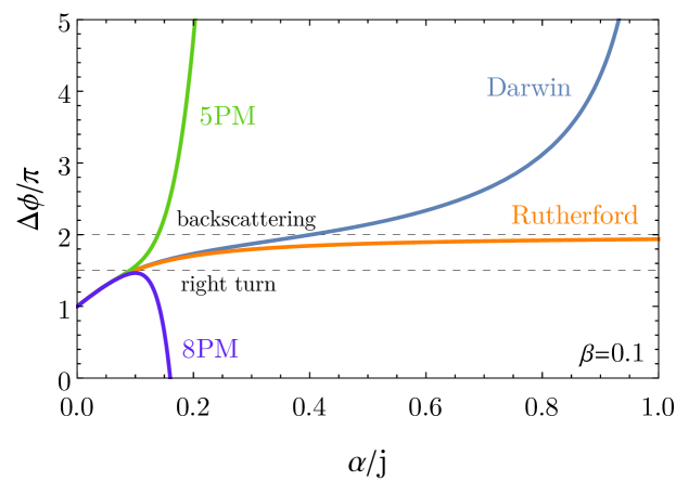
This integral can be carried out analytically, giving exactly the result (29). In figure 1 we plot this scattering angle (denoted by “Darwin”, who was the first to derive it), together with the one for Rutherford scattering, . We also plot the expansions of (29) to 5th and 8th order in . These clearly fail to converge beyond . At this point, the correct scattering angle is , so that the classical trajectory takes a right turn around the origin. This behaviour clearly is not well captured in perturbation theory, unless some sort of resummation is applied.
In this vein, we wish to clarify a few important points about our formalism. Even though it involves a quantum amplitude, it by no means relies on a perturbative expansion. This is in contrast with other methods which rely on an expansion in . This is why we are able to capture classical effects that are inherently non-perturbative from the quantum point of view. The flip side, of course, is that we are working in the probe limit. We will come back to this point, and to future directions away from the probe limit, in the last section.
5 Scalar in Schwarzschild Background
As another application of our semiclassical analysis, we analyze the probe-limit scattering of a scalar in the background of a Schwarzschild BH. To find the phase shifts, we need to solve the Klein-Gordon equation subject to the boundary condition of an incoming wave Teukolsky:1973ha at the BH horizon , where is the Schwarzschild mass and is Newton’s constant. The radial KG equation in a Schwarzschild background is Regge:1957td ; Unruh:1976fm ; Sanchez:1977si ,
| (36) |
with . Again, we made factors of explicit in this equation.
5.1 WKB-Hamilton-Jacobi Analysis
As a first step, we will extract the phase shifts from the WKB approximation to (36). This is guaranteed to reproduce the radial action and classical scattering angle, by virtue of the general map (2). Substituting the WKB ansatz
| (37) |
we get
| (38) |
where . Expanding and (5.1) to first order in , we get
| (39) |
The equation for is exactly the radial Hamilton-Jacobi equation Carter:1968ks ; Carter:1968rr , with playing the role of the radial action where . The formal solution for this radial equation is then
| (40) |
where is the largest real zero of , corresponding to the classical turning point. Correspondingly, we get the ”right of barrier” Ghatak WKB wavefunction
| (41) |
To get the scattering angle, we again use the Hamilton-Jacobi relation
| (42) |
This integral can be carried out analytically, giving the all-order expression to the classical scattering angle of a probe scalar in a Schwarzschild background 111Cf. Scharf for an alternative expression in terms of elliptic functions.
| (43) |
where is the Appell- function (see NIST:DLMF , sec. 16.15). The characteristic radii are defined by
| (44) |
with , and the result is symmetric under . To have a sensible result, we need all three radii to be real, and so the cubic discriminant of has to be non-negative. This, in turn, sets a lower bound on the angular momentum:
| (45) |
Expanding (43) to 4PM order, we get
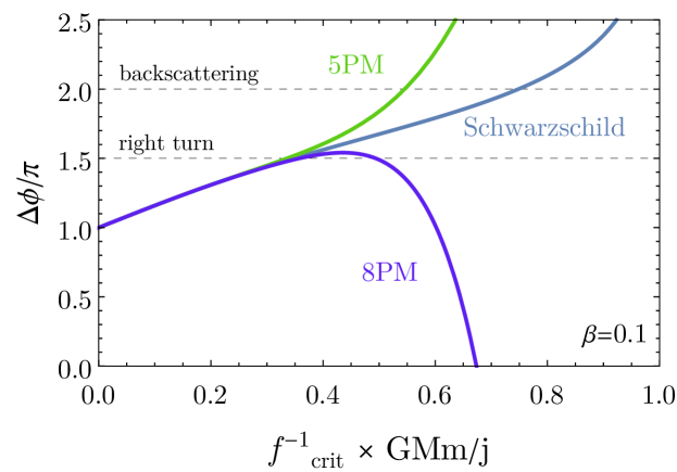
in complete agreement with Bjerrum-Bohr:2014zsa ; Damour:2017zjx . The full scattering angle, as well as its 5PM and 8PM expansions, are depicted in figure 2. As in the Coulomb case, the perturbative expansion fails at , which is approximately when the classical trajectory makes a full right turn around the BH.
5.2 Full Quantum Solution and its Classical Limit
We now wish to relate the full quantum mechanical solution of (36), to the WKB-Hamilton-Jacobi result (40). The relevant boundary condition for this quantum scattering problem is an incoming wave at the BH horizon Teukolsky:1973ha :
| (47) |
To this end we change variables to and substitute the ansatz . Any solution with now satisfies the boundary condition (47). In terms of , the radial equation now becomes
| (48) |
where
| (49) |
This equation is known as a Confluent Heun Equation, and it has a solution
| (50) |
which is defined in Mathematica12 and has a branch cut on the real line for . The full solution to the radial equation is then
| (51) |
and is regular for all . Its asymptotic behavior is given by
| (52) |
where we defined the effective Coulomb parameter , and also .
The phase shifts are not easy to obtain. For small , they can be obtained reliably using the well known method of Mano, Suzuki and Takasugi (MST) Mano:1996mf ; Mano:1996vt . In this method, several different solutions to (48) are expressed as infinite sums of hypergeometric functions, following the seminal work of Leaver:1985 . A solution of (48) that converges at , is obtained as an infinite sum of Gauss Hypergeometric functions. is then expressed as a linear combination of the solutions that converge at , and are in turn given as an infinite sum of Coulomb functions. The MST method has been extensively used in the calculation of both BH perturbations and self-force corrections, see for example Berti:2006wq ; Dolan:2008kf ; Pan:2010hz ; Bini:2013zaa ; Bini:2014zxa ; Damour:2016abl ; Barack:2018yvs
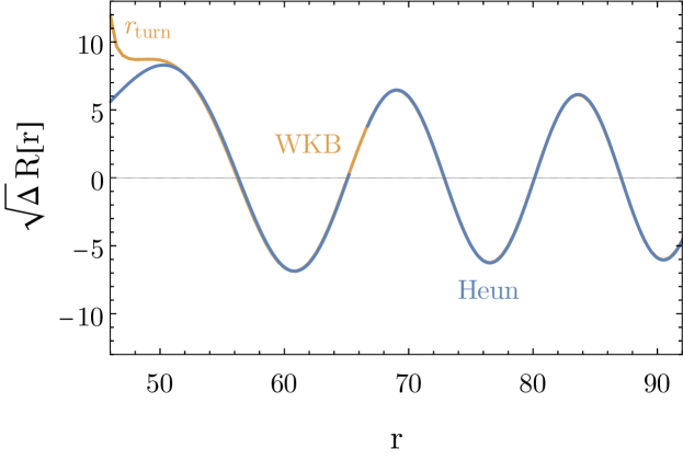
, as well as the living review Sasaki:2003xr . The method is also implemented numerically in the Black hole Perturbation Toolkit code BHPToolkit . However, in the limit we found it somewhat difficult to apply the MST method directly, and we leave it for future work. Instead, we simply plot the full solution (51), together with the WKB solution (41). As can be seen from figure 3, the two functions coincide already when we take . The spike of the WKB seen in the plot is the usual divergence at the classical at the classical turning point - which is usually resolved using an Airy function (see for example Ghatak ). Since we only care about the phase at , we will not dwell on this further.
6 Generalization to Higher Spins and Electric-Magnetic Scattering
The expression (6) can be easily generalized to the case of arbitrary spin particles by means of the Jacob-Wick formula 222See, for example Haber:1994pe ; Baratella:2020dvw and chapter 2 of Pilkuhn:1979ps for pedagogical presentations of the Jacob-Wick formalism. For an on-shell derivation of this formula, see Arkani-Hamed:2017jhn ; Jiang:2020rwz . Jacob:1959at . The scattering amplitude for particles with helicities 333As the particles can be massive, their helicities are not Lorentz invariant. Here we specialize to the COM frame with the incoming particles traveling along the z-axis. is
| (53) |
where are the helicities of the scattered particles, . The normalization is conventionally taken as . Meanwhile, is the famous Wigner matrix, defined as
| (54) |
For simplicity, we will focus on the case where , with . In this case we have, up to a phase,
| (55) |
and . The case in the equation above is easily interpreted in terms of effective one body dynamics: it is the amplitude for a helicity plane wave to scatter into the angle . We will comment on the one body interpretation of below.
Our next step is to take the classical limit, noting that is the classical spin/helicity of the particle which is finite when . Repeating the Poisson summation of (10), we can take the classical limit of the -matrix as worked out by Schwinger et al. in Schwinger:1976fr . Defining and , we have
| (56) |
Where , and For the Schwinger approximation reproduces (11). Plugging the asymptotic form (56) into the Poisson sum, we now get the generalization of (12),
| (57) |
with
| (58) |
Following Schwinger et al. Schwinger:1976fr , we take the stationary phase approximation of , and find that the classical scattering angle is given by
| (59) |
Note that in this case the classical trajectory is not confined to the -plane, and so . However, the relation still holds as a consequence of the WKB-Hamilton-Jacobi analysis.
6.1 Classical Interpretation
To interpret (6), we pick such that the effective one body dynamics is that of a spin particle scattering in a central field. The particle enters with its momentum along and leaves along , with the scattering angle given by . As the particle moves from to , it gets deflected azimuthally by in the plane transverse to , or in other words:
| (60) |
In addition, the motion is constrained by total angular momentum conservation. The total angular momentum in this case is
| (61) |
Since at , we have
| (62) |
The combination of (6.1) and (62), and some elementary trigonometry, leads to
| (63) |
consistently with (6).
6.2 Electric-Magnetic Scattering
In Csaki:2020inw , the Jacob-Wick formula was generalized to the scattering of electric-magnetic scattering, i.e. the scattering of mutually non-local particle like an electric charge and a monopole or two dyons with charges . First, we define the pairwise helicity Csaki:2020uun of the two particles to be the half integer
| (64) |
We also define the corresponding classical quantity . The generalized Jacob-Wick formula is then
| (65) | |||||
The modified -matrices are also known as monopole harmonics Wu:1976ge or spin-weighted spherical harmonics Teukolsky:1973ha . Their appearance reflects the fact that the total angular momentum includes a contribution from the electromagnetic field sourced by the scattering dyons. The generalized Jacob-Wick formula (65) was derived in Csaki:2020inw for fermion-monopole scattering, but it can be shown to hold for all helicities by the same pairwise helicity arguments.
The semiclassical result (6) holds in this case as well. In fact, to obtain the scattering angle for a scalar charge on a scalar monopole, we simply take but . We can now directly apply (6) with and and get Boulware:1976tv ; Schwinger:1976fr
| (66) |
The classical interpretation of this relation is similar to the case, with a slight modification. The total angular momentum is now given by
| (67) |
which means that the entire motion is confined to the cone . Together with (6.1), this immediately gives the result (66).
We can now apply the semiclassical limit to charge-monopole scattering, or equivalently to its gravitational double copy, a probe mass in Newman-Taburino-Unti (NUT) space. We will do this in the next two sections.
7 Charge-Monopole Scattering
By the arguments of the previous section, the classical scattering angle for a scalar charge in the background of a scalar monopole is given by (66), with . To apply it, we need to solve for the phase shifts of a scalar plane wave in the background field of the monopole. To do this, we solve the Klein-Gordon equation (18), with a vector potential given by
| (68) |
and . This potential has a “Dirac string” along the negative axis, but we will see without loss of generality that the test charge always stays in the upper hemisphere, so this will not play a role in our analysis. Of course the formal way to fix this is to define the vector potential on the north and south hemispheres separately Wu:1976ge .
Substituting the vector potential in the KG equation (18), we find
| (69) |
Here the squared angular momentum operator is given by Shnir:2005xx
| (70) |
As expected, this operator is modified by the presence of the angular momentum carried by the EM field. The eigenvalues of are related to our -matrices
| (71) |
where are the complex conjugates of Wigner’s -matrices. Now we can separate variables as and get the radial equation
| (72) |
where and
| (73) |
We recall here the Langer correction Langer of in . Equation (72) a spherical Bessel equation whose regular solution at is . Asymptotically we have
| (74) |
with . Taking the classical limit, we have
| (75) |
By (66), the classical scattering angle is then given by
| (76) |
This all order expression was first derived in Banderet:1946fm ; Schwinger:1976fr ; Boulware:1976tv in a non-relativistic context, and it exactly reproduces the classical calculation of Schwinger:1976fr ; Boulware:1976tv .
7.1 Probe mass in NUT Space
In this section we use our phase shift formalism to derive the all-order classical scattering angle for a probe mass (equivalently, a probe Schwarzschild BH) in the background of a pure NUT, i.e. the limit bonnor1969 of Taub-NUT space Taub:1950ez ; NUT . NUT space is the double copy of a magnetic monopole Luna:2015paa ; Caron-Huot:2018ape ; Huang:2019cja ; Alawadhi:2019urr ; Kol:2020ucd ; Moynihan:2020gxj ; Emond:2020lwi ; Kim:2020cvf ; Alawadhi:2021uie , and so this problem is the double copy of charge-monopole scattering.
The metric for Taub-NUT space in Boyer-Lindquist coordinates is given by
| (77) |
where is the mass and in the NUT charge while
| (78) |
Here we use the upper hemisphere metric of Kol:2020ucd . The pure NUT metric is then obtained by setting (conversely, in the limit the metric reduces to the Schwarzschild metric).
As we will show explicitly below, when considering the scattering of a test mass in NUT space, regularity of the angular wavefuctions at the Misner string Misner:1963fr (here on the negative -axis) requires the quantization of
| (79) |
in half-integer units (see also Dowker1974 for a similar conclusion). This is a further validation of the classical double copy relation between mass-NUT scattering and charge-monopole scattering Luna:2015paa ; Huang:2019cja ; Alawadhi:2019urr ; Kol:2020ucd ; Moynihan:2020gxj ; Emond:2020lwi ; Kim:2020cvf ; Alawadhi:2021uie - this time in terms of an inherently non-perturbative quantization condition. In complete analogy with the charge-monopole case, the gravitational field sourced by the NUT and the probe mass contains additional angular momentum , where is the unit vector from the NUT to the probe mass. This has been shown classically a long time ago bonnor1969 ; Dowker1974 ; Zimmerman1989 ; Kagramanova:2010bk ; Clement:2015cxa ; Frolov:2017kze .
Note that this angular momentum is proportional to the overall energy of the probe mass and not its rest mass, which we can take to be small or even zero. In other words, this is not a gravitational backreaction effect from the mass of the probe, but rather the net angular momentum carried by the soft gravitons exchanged between the NUT and the probe.
Consequently, the modified Jacob-Wick formula (65) is also valid in the mass-NUT case, with appropriate phase shifts . To compute these phase shifts, we solve the Klein-Gordon equation
| (80) |
in the background (77). Writing the D’Alembertian explicitly and substituting the ansatz , we get
| (81) |
Here , and the squared angular momentum operator is given by the same expression as the monopole case, (70), whose eigenfunctions are . Now we can separate variables as
| (82) |
and find (cf. Dowker1974 ; Bini:2003sy )
| (83) |
We will now solve this equation and extract the classical scattering angle in two ways: first, by the WKB-Hamilton-Jacobi method, followed by taking the classical limit of the full quantum solution.
7.2 WKB-Hamilton-Jacobi Analysis
Substituting the WKB ansatz , we deduce the radial Hamilton-Jacobi equation Carter:1968rr ; Zimmerman1989 ; Kagramanova:2010bk ; Clement:2015cxa ; Frolov:2017kze . To leading order in , this is
| (84) |
The formal solution for this radial equation is then
| (85) |
where is the largest real zero of , corresponding to the classical turning point. To determine the scattering angle, we use the Hamilton-Jacobi relation
| (86) |
The above integral can be carried out analytically, giving the all-order expression to the classical scattering angle of a probe scalar in a NUT background
| (87) |
where is Legendre’s complete elliptic integral, and in this case it is a function of . Note that in Mathematica, elliptic integrals are expressed as functions of . The characteristic radii are defined by
| (88) |
with . Explicitly, are
| (89) |
Expanding to 6PM order, we find
| (90) | |||||
It is nice to note that this expression is consistent with the 2PM result obtained by on-shell methods in Kim:2020cvf . This resolves the apparent discrepancy in Kim:2020cvf in a simple way - by evaluating the integral (86) analytically as an elliptic integral.
7.3 Full Quantum Solution and its Classical Limit
Here we find the exact phase shifts of the full quantum problem, and show that their classical limit reproduces (87). Changing variables in (83) as with , and remembering that , we deduce the radial equation
| (91) |
where
| (92) |
and . This is a prolate spheroidal equation with a complex separation constant - a very well studied equation meixner2006mathieu ; arscott1964periodic ; Falloon_2003 . The solution we are looking for is the one which satisfies an absorbing boundary condition at Teukolsky:1973ha :
| (93) |
Here is the “tortoise” coordinate Eddington ; Regge:1957td ; Finkelstein , which satisfies . This solution is conventionally denoted by . The parameter is the index of the radial spheroidal function, and is related to and by a transcendental equation, which is explicitly given in Appendix A. We explicitly checked that the other solution to the radial equation, , only leads to quantum corrections that die off in the limit. The asymptotic behavior of the solution at is given by
| (94) |
In appendix A we show how to calculate explicitly. By a similar argument to the monopole case, we have and so the classical scattering angle is given by
| (95) |
where
| (96) |
and is given to all orders in appendix A. This expression coincides to all orders with the one obtained by the WKB-Hamilton-Jacobi method, equation (87).
Note that although the consistency of (96) and (87) is guaranteed by the correspondence principle between quantum and classical physics at , the actual all-order equality involves a highly non-trivial number theoretical identity:
| (97) |
or in other words
| (98) |
where and is . Here is given implicitly as the value which solves
| (99) |
where . The function is known in the literature as the (analytically continued) spheroidal eigenvalue meixner2006mathieu ; Falloon_2003 . Here we uncover a very non-trivial relation between its derivative in the limit and the elliptic integral . We are not aware of previous derivations of this relation in the literature.
8 Outlook: Towards Non-Perturbative Self-Force Calculations
Our results clearly demonstrate that classical effects that appear to be non-perturbative in the PM expansion can be fully captured in the limit of quantum wave equations. In and of itself, this should not surprise the reader much, as it is a consequence of the correspondence principle between quantum and classical physics. However, we uncovered in detail exactly how the quantum amplitude encodes the classical scattering data in the limit, namely
-
•
The phase shifts go over to their WKB-Hamilton-Jacobi values, which are in turn related to the classical radial action by (2).
- •
We applied this formalism in the probe limit to calculate classical effects that are inherently non-perturbative from the qunatum point of view. For example, we reproduced the winding of classical trajectories for relativistic Coulomb and Schwarzschild scattering, as well as the effect of the extra angular momentum in the gravitational (electromagnetic) field for probe mass-NUT (charge-monopole) scattering. In the two latter cases, we also correctly reproduced the fact that the classical trajectories are confined to a cone around the total angular momentum .
Finally, our quantum-classical matching uncovers previously unknown (to us) number-theoretic relations such as (98). We expect a similar number-theoretic relation to hold in the context of probe scattering off Schwarzschild: that is, between the phase shift emerging from the HeunC function, and the Appell F1 function which we know describes the classical trajectory.
An obvious direction for future work is to apply similar methods to black hole scattering away from the probe limit, i.e. to all orders in but perturbatively in . In other words, it would be interesting to apply our method to calculate “self-force” corrections. Since our method is non-perturbative in , its application away from the probe limit will inevitably involve both energy loss to radiation and conservative tail effects that are nonlocal in time BonnorRotenberg66 ; BlanchetDamour86 ; BlanchetDamourTail ; BlanchetDamour92 ; Blanchet_1993 ; Blanchet:1997jj ; Asada:1997zu ; Galley:2015kus ; Marchand:2016vox .
One possible way forward would be to consider quantum scattering in the full Arnowitt-Deser-Misner Hamiltonian ADM ; Schafer:2018kuf , without integrating out the gravitational field. This would lead to a set of coupled wave equations for the two black holes and the gravitational field, which could be solved to all orders in but order-by-order in . To focus on conservative dynamics, we could impose the boundary condition of a pure Schwarzschild metric at , such that there is no leakage of energy via gravitational waves. However, tail effect will be captured since outgoing gravitational waves would be reflected back to the center by the ambient Schwarzschild metric in the far zone.
Calculating self-force corrections in terms of wave equations would have the additional advantage of smoothing out the inherent divergences which are ubiquitous in coupling point masses to GR, which requires very careful regularization in the standard treatments Barack:1999wf ; Blanchet:2000cw ; Damour:2001bu ; Blanchet:2013haa ; Schafer:2018kuf ; Barack:2018yly ; Barack:2018yvs .
Turning away from gravitational wave physics, our methods may have an application to the study of the double copy beyond perturbation theory Monteiro:2014cda ; Luna:2015paa ; Adamo:2017nia ; Adamo:2018mpq ; Monteiro:2020plf ; Campiglia:2021srh ; Borsten:2021hua ; Chacon:2021wbr ; Gonzo:2021drq ; Godazgar:2021iae ; Adamo:2021dfg . It is by now well-established that a pure NUT is related to the magnetic monopole by the double copy in perturbation theory; indeed, this was an initial motivation for our work on the pure NUT. We have now seen how to construct amplitudes for monopoles and NUTs to all orders, so we have the theoretical data to explore this double copy to all orders. Of course this would just be a prelude to the study of the double copy relating a charge and Schwarzschild to all orders.
Acknowledgements
We thank Yu-tin Huang for many helpful discussions, Mao Zeng for insightful and encouraging correspondence, and Andrés Luna for reading our manuscript and pointing out a clerical error in a key formula. We thank the Galileo Galilei Institute for Theoretical Physics (GGI) for hosting a workshop, conference and training week on “Gravitational scattering, inspiral, and radiation” which informed and enriched our work. DOC is supported by the STFC grant ST/P0000630/1. OT is supported in part by the DOE under grant DE-AC02-05CH11231.
Appendix A Characteristic Equation for the NUT Spheroidal Equation
In this appendix we calculate the index for the prolate spheroidal equation Eq. 91. The index is linked to the scattering phase shift by . The index is related to the parameters of the spheroidal equation by a transcendetal equation. Following Falloon_2003 , we define the following variables:
| (100) |
as well as
| (101) |
The variables and for NUT scattering are defined in (92). In this appendix is an integer index, not to be confused with the plane wave momentum . In terms of , , we define two continued fractions, whose sum is required to vanish. These are
| (102) |
The transcendental equation for is then given by
| (103) |
Note that it is usually treated as an equation for , which is known as the “spheroidal eigenvalue” of the problem. In this case the index is treated as an integer enumerating the eigenvalue . In particular, and related by Eq. 103 satisfy the continuity relation . Here we use the same machinery in a different manner, by fixing and solving for . It is particularly useful for our purposes to substitute an ansatz for of the form
| (104) |
We can solve for the coefficients explicitly by substituing this ansatz in the transcendental relation (103). The first 4 coefficients (corresponding to a 6PM expansion) are then
| (105) |
See (92) for the definitions of .
References
- (1) L. Blanchet, T. Damour, G. Esposito-Farese, and B. R. Iyer, Gravitational radiation from inspiralling compact binaries completed at the third post-Newtonian order, Phys. Rev. Lett. 93 (2004) 091101, [gr-qc/0406012].
- (2) R. A. Porto, The effective field theorist’s approach to gravitational dynamics, Phys. Rept. 633 (2016) 1–104, [arXiv:1601.04914].
- (3) M. Levi, Effective Field Theories of Post-Newtonian Gravity: A comprehensive review, Rept. Prog. Phys. 83 (2020), no. 7 075901, [arXiv:1807.01699].
- (4) D. Bini, T. Damour, and A. Geralico, Sixth post-Newtonian nonlocal-in-time dynamics of binary systems, Phys. Rev. D 102 (2020), no. 8 084047, [arXiv:2007.11239].
- (5) D. Bini, T. Damour, and A. Geralico, Sixth post-Newtonian local-in-time dynamics of binary systems, Phys. Rev. D 102 (2020), no. 2 024061, [arXiv:2004.05407].
- (6) D. Bini, T. Damour, A. Geralico, S. Laporta, and P. Mastrolia, Gravitational scattering at the seventh order in : nonlocal contribution at the sixth post-Newtonian accuracy, Phys. Rev. D 103 (2021), no. 4 044038, [arXiv:2012.12918].
- (7) D. Bini, T. Damour, A. Geralico, S. Laporta, and P. Mastrolia, Gravitational dynamics at : perturbative gravitational scattering meets experimental mathematics, arXiv:2008.09389.
- (8) D. Bini, T. Damour, and A. Geralico, Binary dynamics at the fifth and fifth-and-a-half post-Newtonian orders, Phys. Rev. D 102 (2020), no. 2 024062, [arXiv:2003.11891].
- (9) D. Bini, T. Damour, and A. Geralico, Radiative contributions to gravitational scattering, arXiv:2107.08896.
- (10) A. Buonanno and T. Damour, Effective one-body approach to general relativistic two-body dynamics, Phys. Rev. D 59 (1999) 084006, [gr-qc/9811091].
- (11) A. Buonanno and T. Damour, Transition from inspiral to plunge in binary black hole coalescences, Phys. Rev. D 62 (2000) 064015, [gr-qc/0001013].
- (12) T. Damour, Coalescence of two spinning black holes: an effective one-body approach, Phys. Rev. D 64 (2001) 124013, [gr-qc/0103018].
- (13) T. Damour, P. Jaranowski, and G. Schaefer, Effective one body approach to the dynamics of two spinning black holes with next-to-leading order spin-orbit coupling, Phys. Rev. D 78 (2008) 024009, [arXiv:0803.0915].
- (14) K. G. Arun, A. Buonanno, G. Faye, and E. Ochsner, Higher-order spin effects in the amplitude and phase of gravitational waveforms emitted by inspiraling compact binaries: Ready-to-use gravitational waveforms, Phys. Rev. D 79 (2009) 104023, [arXiv:0810.5336]. [Erratum: Phys.Rev.D 84, 049901 (2011)].
- (15) T. Damour and A. Nagar, An Improved analytical description of inspiralling and coalescing black-hole binaries, Phys. Rev. D 79 (2009) 081503, [arXiv:0902.0136].
- (16) T. Damour and A. Nagar, Effective One Body description of tidal effects in inspiralling compact binaries, Phys. Rev. D 81 (2010) 084016, [arXiv:0911.5041].
- (17) Y. Pan, A. Buonanno, R. Fujita, E. Racine, and H. Tagoshi, Post-Newtonian factorized multipolar waveforms for spinning, non-precessing black-hole binaries, Phys. Rev. D 83 (2011) 064003, [arXiv:1006.0431]. [Erratum: Phys.Rev.D 87, 109901 (2013)].
- (18) A. Taracchini et al., Effective-one-body model for black-hole binaries with generic mass ratios and spins, Phys. Rev. D 89 (2014), no. 6 061502, [arXiv:1311.2544].
- (19) D. Bini and T. Damour, Gravitational self-force corrections to two-body tidal interactions and the effective one-body formalism, Phys. Rev. D 90 (2014), no. 12 124037, [arXiv:1409.6933].
- (20) A. Nagar, F. Messina, C. Kavanagh, G. Lukes-Gerakopoulos, N. Warburton, S. Bernuzzi, and E. Harms, Factorization and resummation: A new paradigm to improve gravitational wave amplitudes. III: the spinning test-body terms, Phys. Rev. D 100 (2019), no. 10 104056, [arXiv:1907.12233].
- (21) A. Antonelli, M. van de Meent, A. Buonanno, J. Steinhoff, and J. Vines, Quasicircular inspirals and plunges from nonspinning effective-one-body Hamiltonians with gravitational self-force information, Phys. Rev. D 101 (2020), no. 2 024024, [arXiv:1907.11597].
- (22) A. Nagar, G. Pratten, G. Riemenschneider, and R. Gamba, Multipolar effective one body model for nonspinning black hole binaries, Phys. Rev. D 101 (2020), no. 2 024041, [arXiv:1904.09550].
- (23) S. Albanesi, A. Nagar, and S. Bernuzzi, Effective one-body model for extreme-mass-ratio spinning binaries on eccentric equatorial orbits: Testing radiation reaction and waveform, Phys. Rev. D 104 (2021), no. 2 024067, [arXiv:2104.10559].
- (24) N. E. J. Bjerrum-Bohr, J. F. Donoghue, and P. Vanhove, On-shell Techniques and Universal Results in Quantum Gravity, JHEP 02 (2014) 111, [arXiv:1309.0804].
- (25) N. E. J. Bjerrum-Bohr, J. F. Donoghue, B. R. Holstein, L. Planté, and P. Vanhove, Bending of Light in Quantum Gravity, Phys. Rev. Lett. 114 (2015), no. 6 061301, [arXiv:1410.7590].
- (26) J. Vines, Scattering of two spinning black holes in post-Minkowskian gravity, to all orders in spin, and effective-one-body mappings, Class. Quant. Grav. 35 (2018), no. 8 084002, [arXiv:1709.06016].
- (27) N. E. J. Bjerrum-Bohr, P. H. Damgaard, G. Festuccia, L. Planté, and P. Vanhove, General Relativity from Scattering Amplitudes, Phys. Rev. Lett. 121 (2018), no. 17 171601, [arXiv:1806.04920].
- (28) C. Cheung, I. Z. Rothstein, and M. P. Solon, From Scattering Amplitudes to Classical Potentials in the Post-Minkowskian Expansion, Phys. Rev. Lett. 121 (2018), no. 25 251101, [arXiv:1808.02489].
- (29) J. Vines, J. Steinhoff, and A. Buonanno, Spinning-black-hole scattering and the test-black-hole limit at second post-Minkowskian order, Phys. Rev. D 99 (2019), no. 6 064054, [arXiv:1812.00956].
- (30) P. H. Damgaard, K. Haddad, and A. Helset, Heavy Black Hole Effective Theory, JHEP 11 (2019) 070, [arXiv:1908.10308].
- (31) A. Cristofoli, N. E. J. Bjerrum-Bohr, P. H. Damgaard, and P. Vanhove, Post-Minkowskian Hamiltonians in general relativity, Phys. Rev. D 100 (2019), no. 8 084040, [arXiv:1906.01579].
- (32) N. E. J. Bjerrum-Bohr, A. Cristofoli, P. H. Damgaard, and H. Gomez, Scalar-Graviton Amplitudes, JHEP 11 (2019) 148, [arXiv:1908.09755].
- (33) A. Antonelli, A. Buonanno, J. Steinhoff, M. van de Meent, and J. Vines, Energetics of two-body Hamiltonians in post-Minkowskian gravity, Phys. Rev. D 99 (2019), no. 10 104004, [arXiv:1901.07102].
- (34) A. Brandhuber and G. Travaglini, On higher-derivative effects on the gravitational potential and particle bending, JHEP 01 (2020) 010, [arXiv:1905.05657].
- (35) A. Guevara, A. Ochirov, and J. Vines, Black-hole scattering with general spin directions from minimal-coupling amplitudes, Phys. Rev. D 100 (2019), no. 10 104024, [arXiv:1906.10071].
- (36) B. Maybee, D. O’Connell, and J. Vines, Observables and amplitudes for spinning particles and black holes, JHEP 12 (2019) 156, [arXiv:1906.09260].
- (37) N. Arkani-Hamed, Y.-t. Huang, and D. O’Connell, Kerr black holes as elementary particles, JHEP 01 (2020) 046, [arXiv:1906.10100].
- (38) P. Di Vecchia, A. Luna, S. G. Naculich, R. Russo, G. Veneziano, and C. D. White, A tale of two exponentiations in supergravity, Phys. Lett. B 798 (2019) 134927, [arXiv:1908.05603].
- (39) N. E. J. Bjerrum-Bohr, A. Cristofoli, and P. H. Damgaard, Post-Minkowskian Scattering Angle in Einstein Gravity, JHEP 08 (2020) 038, [arXiv:1910.09366].
- (40) P. Di Vecchia, S. G. Naculich, R. Russo, G. Veneziano, and C. D. White, A tale of two exponentiations in = 8 supergravity at subleading level, JHEP 03 (2020) 173, [arXiv:1911.11716].
- (41) M.-Z. Chung, Y.-T. Huang, and J.-W. Kim, Classical potential for general spinning bodies, JHEP 09 (2020) 074, [arXiv:1908.08463].
- (42) T. Damour, Radiative contribution to classical gravitational scattering at the third order in , Phys. Rev. D 102 (2020), no. 12 124008, [arXiv:2010.01641].
- (43) A. Cristofoli, P. H. Damgaard, P. Di Vecchia, and C. Heissenberg, Second-order Post-Minkowskian scattering in arbitrary dimensions, JHEP 07 (2020) 122, [arXiv:2003.10274].
- (44) G. Kälin, Z. Liu, and R. A. Porto, Conservative Dynamics of Binary Systems to Third Post-Minkowskian Order from the Effective Field Theory Approach, Phys. Rev. Lett. 125 (2020), no. 26 261103, [arXiv:2007.04977].
- (45) C. Cheung and M. P. Solon, Classical gravitational scattering at (G3) from Feynman diagrams, JHEP 06 (2020) 144, [arXiv:2003.08351].
- (46) G. Kälin and R. A. Porto, Post-Minkowskian Effective Field Theory for Conservative Binary Dynamics, JHEP 11 (2020) 106, [arXiv:2006.01184].
- (47) P. Di Vecchia, C. Heissenberg, R. Russo, and G. Veneziano, Universality of ultra-relativistic gravitational scattering, Phys. Lett. B 811 (2020) 135924, [arXiv:2008.12743].
- (48) L. de la Cruz, B. Maybee, D. O’Connell, and A. Ross, Classical Yang-Mills observables from amplitudes, JHEP 12 (2020) 076, [arXiv:2009.03842].
- (49) M. Accettulli Huber, A. Brandhuber, S. De Angelis, and G. Travaglini, From amplitudes to gravitational radiation with cubic interactions and tidal effects, Phys. Rev. D 103 (2021), no. 4 045015, [arXiv:2012.06548].
- (50) A. Guevara, B. Maybee, A. Ochirov, D. O’connell, and J. Vines, A worldsheet for Kerr, JHEP 03 (2021) 201, [arXiv:2012.11570].
- (51) P. Di Vecchia, C. Heissenberg, R. Russo, and G. Veneziano, Radiation Reaction from Soft Theorems, Phys. Lett. B 818 (2021) 136379, [arXiv:2101.05772].
- (52) Y. F. Bautista, A. Guevara, C. Kavanagh, and J. Vines, From Scattering in Black Hole Backgrounds to Higher-Spin Amplitudes: Part I, arXiv:2107.10179.
- (53) P. H. Damgaard and P. Vanhove, Remodeling the Effective One-Body Formalism in Post-Minkowskian Gravity, arXiv:2108.11248.
- (54) N. E. J. Bjerrum-Bohr, P. H. Damgaard, L. Planté, and P. Vanhove, The Amplitude for Classical Gravitational Scattering at Third Post-Minkowskian Order, arXiv:2105.05218.
- (55) N. E. J. Bjerrum-Bohr, P. H. Damgaard, L. Planté, and P. Vanhove, Classical gravity from loop amplitudes, Phys. Rev. D 104 (2021), no. 2 026009, [arXiv:2104.04510].
- (56) P. Di Vecchia, C. Heissenberg, R. Russo, and G. Veneziano, The eikonal approach to gravitational scattering and radiation at (G3), JHEP 07 (2021) 169, [arXiv:2104.03256].
- (57) Z. Liu, R. A. Porto, and Z. Yang, Spin Effects in the Effective Field Theory Approach to Post-Minkowskian Conservative Dynamics, JHEP 06 (2021) 012, [arXiv:2102.10059].
- (58) A. Brandhuber, G. Chen, G. Travaglini, and C. Wen, A new gauge-invariant double copy for heavy-mass effective theory, JHEP 07 (2021) 047, [arXiv:2104.11206].
- (59) C. Dlapa, G. Kälin, Z. Liu, and R. A. Porto, Dynamics of Binary Systems to Fourth Post-Minkowskian Order from the Effective Field Theory Approach, arXiv:2106.08276.
- (60) A. Cristofoli, R. Gonzo, D. A. Kosower, and D. O’Connell, Waveforms from Amplitudes, arXiv:2107.10193.
- (61) A. Brandhuber, G. Chen, G. Travaglini, and C. Wen, Classical gravitational scattering from a gauge-invariant double copy, arXiv:2108.04216.
- (62) W. D. Goldberger and I. Z. Rothstein, An Effective field theory of gravity for extended objects, Phys. Rev. D 73 (2006) 104029, [hep-th/0409156].
- (63) W. D. Goldberger and I. Z. Rothstein, Dissipative effects in the worldline approach to black hole dynamics, Phys. Rev. D 73 (2006) 104030, [hep-th/0511133].
- (64) T. Damour, High-energy gravitational scattering and the general relativistic two-body problem, Phys. Rev. D 97 (2018), no. 4 044038, [arXiv:1710.10599].
- (65) T. Damour, Classical and quantum scattering in post-Minkowskian gravity, Phys. Rev. D 102 (2020), no. 2 024060, [arXiv:1912.02139].
- (66) A. Guevara, Holomorphic Classical Limit for Spin Effects in Gravitational and Electromagnetic Scattering, JHEP 04 (2019) 033, [arXiv:1706.02314].
- (67) D. A. Kosower, B. Maybee, and D. O’Connell, Amplitudes, Observables, and Classical Scattering, JHEP 02 (2019) 137, [arXiv:1811.10950].
- (68) J. F. Donoghue, Leading quantum correction to the Newtonian potential, Phys. Rev. Lett. 72 (1994) 2996–2999, [gr-qc/9310024].
- (69) J. F. Donoghue, General relativity as an effective field theory: The leading quantum corrections, Phys. Rev. D 50 (1994) 3874–3888, [gr-qc/9405057].
- (70) D. Neill and I. Z. Rothstein, Classical Space-Times from the S Matrix, Nucl. Phys. B 877 (2013) 177–189, [arXiv:1304.7263].
- (71) F. Cachazo and A. Guevara, Leading Singularities and Classical Gravitational Scattering, JHEP 02 (2020) 181, [arXiv:1705.10262].
- (72) Z. Bern, L. J. Dixon, D. C. Dunbar, and D. A. Kosower, Fusing gauge theory tree amplitudes into loop amplitudes, Nucl. Phys. B 435 (1995) 59–101, [hep-ph/9409265].
- (73) Z. Bern, L. J. Dixon, D. C. Dunbar, and D. A. Kosower, One loop n point gauge theory amplitudes, unitarity and collinear limits, Nucl. Phys. B 425 (1994) 217–260, [hep-ph/9403226].
- (74) Z. Bern, J. J. M. Carrasco, and H. Johansson, New Relations for Gauge-Theory Amplitudes, Phys. Rev. D 78 (2008) 085011, [arXiv:0805.3993].
- (75) Z. Bern, J. J. M. Carrasco, and H. Johansson, Perturbative Quantum Gravity as a Double Copy of Gauge Theory, Phys. Rev. Lett. 105 (2010) 061602, [arXiv:1004.0476].
- (76) Z. Bern, T. Dennen, Y.-t. Huang, and M. Kiermaier, Gravity as the Square of Gauge Theory, Phys. Rev. D 82 (2010) 065003, [arXiv:1004.0693].
- (77) A. V. Smirnov, Algorithm FIRE – Feynman Integral REduction, JHEP 10 (2008) 107, [arXiv:0807.3243].
- (78) Z. Bern, C. Cheung, R. Roiban, C.-H. Shen, M. P. Solon, and M. Zeng, Black Hole Binary Dynamics from the Double Copy and Effective Theory, JHEP 10 (2019) 206, [arXiv:1908.01493].
- (79) Z. Bern, C. Cheung, R. Roiban, C.-H. Shen, M. P. Solon, and M. Zeng, Scattering Amplitudes and the Conservative Hamiltonian for Binary Systems at Third Post-Minkowskian Order, Phys. Rev. Lett. 122 (2019), no. 20 201603, [arXiv:1901.04424].
- (80) Z. Bern, A. Luna, R. Roiban, C.-H. Shen, and M. Zeng, Spinning black hole binary dynamics, scattering amplitudes, and effective field theory, Phys. Rev. D 104 (2021), no. 6 065014, [arXiv:2005.03071].
- (81) Z. Bern, H. Ita, J. Parra-Martinez, and M. S. Ruf, Universality in the classical limit of massless gravitational scattering, Phys. Rev. Lett. 125 (2020), no. 3 031601, [arXiv:2002.02459].
- (82) Z. Bern, J. Parra-Martinez, R. Roiban, M. S. Ruf, C.-H. Shen, M. P. Solon, and M. Zeng, Scattering Amplitudes and Conservative Binary Dynamics at , Phys. Rev. Lett. 126 (2021), no. 17 171601, [arXiv:2101.07254].
- (83) W. B. Bonnor and M. A. Rotenberg, Gravitational waves from isolated sources, Proceedings of the Royal Society of London. Series A. Mathematical and Physical Sciences 289 (1966), no. 1417 247–274.
- (84) L. Blanchet and T. Damour, Radiative gravitational fields in general relativity. I - General structure of the field outside the source, Philosophical Transactions of the Royal Society of London Series A 320 (1986), no. 1555 379–430.
- (85) L. Blanchet and T. Damour, Tail-transported temporal correlations in the dynamics of a gravitating system, Phys. Rev. D 37 (1988) 1410–1435.
- (86) L. Blanchet and T. Damour, Hereditary effects in gravitational radiation, Phys. Rev. D 46 (1992) 4304–4319.
- (87) L. Blanchet and G. Schafer, Gravitational wave tails and binary star systems, Classical and Quantum Gravity 10 (1993), no. 12 2699–2721.
- (88) L. Blanchet, Gravitational wave tails of tails, Class. Quant. Grav. 15 (1998) 113–141, [gr-qc/9710038]. [Erratum: Class.Quant.Grav. 22, 3381 (2005)].
- (89) H. Asada and T. Futamase, Propagation of gravitational waves from slow motion sources in Coulomb type potential, Phys. Rev. D 56 (1997) R6062–R6066, [gr-qc/9711009].
- (90) C. R. Galley, A. K. Leibovich, R. A. Porto, and A. Ross, Tail effect in gravitational radiation reaction: Time nonlocality and renormalization group evolution, Phys. Rev. D 93 (2016) 124010, [arXiv:1511.07379].
- (91) T. Marchand, L. Blanchet, and G. Faye, Gravitational-wave tail effects to quartic non-linear order, Class. Quant. Grav. 33 (2016), no. 24 244003, [arXiv:1607.07601].
- (92) L. Landau and E. Lifshitz, Mechanics: Volume 1. No. v. 1. Elsevier Science, 1982.
- (93) G. Kälin and R. A. Porto, From boundary data to bound states. Part II. Scattering angle to dynamical invariants (with twist), JHEP 02 (2020) 120, [arXiv:1911.09130].
- (94) G. Kälin and R. A. Porto, From Boundary Data to Bound States, JHEP 01 (2020) 072, [arXiv:1910.03008].
- (95) G. Kälin, Z. Liu, and R. A. Porto, Conservative Tidal Effects in Compact Binary Systems to Next-to-Leading Post-Minkowskian Order, Phys. Rev. D 102 (2020) 124025, [arXiv:2008.06047].
- (96) W. G. Unruh, Absorption Cross-Section of Small Black Holes, Phys. Rev. D 14 (1976) 3251–3259.
- (97) N. G. Sanchez, Absorption and Emission Spectra of a Schwarzschild Black Hole, Phys. Rev. D 18 (1978) 1030.
- (98) N. G. Sanchez, Elastic Scattering of Waves by a Black Hole, Phys. Rev. D 18 (1978) 1798.
- (99) S. A. Teukolsky, Perturbations of a rotating black hole. 1. Fundamental equations for gravitational electromagnetic and neutrino field perturbations, Astrophys. J. 185 (1973) 635–647.
- (100) S. Teukolsky and W. Press, Perturbations of a rotating black hole. III - Interaction of the hole with gravitational and electromagnet ic radiation, Astrophys. J. 193 (1974) 443–461.
- (101) K. W. Ford and J. A. Wheeler, Application of semiclassical scattering analysis, Annals of Physics 7 (1959), no. 3 287–322.
- (102) M. V. Berry and K. E. Mount, Semiclassical approximations in wave mechanics, Reports on Progress in Physics 35 (1972).
- (103) G. Mogull, J. Plefka, and J. Steinhoff, Classical black hole scattering from a worldline quantum field theory, JHEP 02 (2021) 048, [arXiv:2010.02865].
- (104) G. U. Jakobsen, G. Mogull, J. Plefka, and J. Steinhoff, Classical Gravitational Bremsstrahlung from a Worldline Quantum Field Theory, Phys. Rev. Lett. 126 (2021), no. 20 201103, [arXiv:2101.12688].
- (105) C. Shi and J. Plefka, Classical Double Copy of Worldline Quantum Field Theory, arXiv:2109.10345.
- (106) J. T. M. F.R.S., Xxxiv. on momentum in the electric field, The London, Edinburgh, and Dublin Philosophical Magazine and Journal of Science 8 (1904), no. 45 331–356.
- (107) H. Lipkin, W. Weisberger, and M. Peshkin, Magnetic charge quantization and angular momentum, Annals Phys. 53 (1969) 203–214.
- (108) D. G. Boulware, L. S. Brown, R. N. Cahn, S. Ellis, and C.-k. Lee, Scattering on Magnetic Charge, Phys. Rev. D 14 (1976) 2708.
- (109) J. S. Schwinger, K. A. Milton, W.-y. Tsai, L. L. DeRaad, Jr., and D. C. Clark, Nonrelativistic Dyon-Dyon Scattering, Annals Phys. 101 (1976) 451.
- (110) Y. M. Shnir, Magnetic Monopoles. Springer Berlin Heidelberg, 2005.
- (111) C. Csaki, S. Hong, Y. Shirman, O. Telem, J. Terning, and M. Waterbury, Scattering Amplitudes for Monopoles: Pairwise Little Group and Pairwise Helicity, arXiv:2009.14213.
- (112) C. Csáki, S. Hong, Y. Shirman, O. Telem, and J. Terning, Multi-particle Representations of the Poincaré Group, arXiv:2010.13794.
- (113) A. Luna, R. Monteiro, D. O’Connell, and C. D. White, The classical double copy for Taub–NUT spacetime, Phys. Lett. B 750 (2015) 272–277, [arXiv:1507.01869].
- (114) S. Caron-Huot and Z. Zahraee, Integrability of Black Hole Orbits in Maximal Supergravity, JHEP 07 (2019) 179, [arXiv:1810.04694].
- (115) Y.-T. Huang, U. Kol, and D. O’Connell, Double copy of electric-magnetic duality, Phys. Rev. D 102 (2020), no. 4 046005, [arXiv:1911.06318].
- (116) R. Alawadhi, D. S. Berman, B. Spence, and D. Peinador Veiga, S-duality and the double copy, JHEP 03 (2020) 059, [arXiv:1911.06797].
- (117) U. Kol and M. Porrati, Gravitational Wu-Yang Monopoles, Phys. Rev. D 101 (2020), no. 12 126009, [arXiv:2003.09054].
- (118) N. Moynihan and J. Murugan, On-Shell Electric-Magnetic Duality and the Dual Graviton, arXiv:2002.11085.
- (119) W. T. Emond, Y.-T. Huang, U. Kol, N. Moynihan, and D. O’Connell, Amplitudes from Coulomb to Kerr-Taub-NUT, arXiv:2010.07861.
- (120) J.-W. Kim and M. Shim, Gravitational Dyonic Amplitude at One-Loop and its Inconsistency with the Classical Impulse, arXiv:2010.14347.
- (121) R. Alawadhi, D. S. Berman, C. D. White, and S. Wikeley, The single copy of the gravitational holonomy, arXiv:2107.01114.
- (122) Y. Mino, M. Sasaki, and T. Tanaka, Gravitational radiation reaction to a particle motion, Phys. Rev. D 55 (1997) 3457–3476, [gr-qc/9606018].
- (123) T. C. Quinn and R. M. Wald, An Axiomatic approach to electromagnetic and gravitational radiation reaction of particles in curved space-time, Phys. Rev. D 56 (1997) 3381–3394, [gr-qc/9610053].
- (124) L. Barack and A. Ori, Mode sum regularization approach for the selfforce in black hole space-time, Phys. Rev. D 61 (2000) 061502, [gr-qc/9912010].
- (125) L. Barack, Y. Mino, H. Nakano, A. Ori, and M. Sasaki, Calculating the gravitational selfforce in Schwarzschild space-time, Phys. Rev. Lett. 88 (2002) 091101, [gr-qc/0111001].
- (126) S. L. Detweiler and B. F. Whiting, Selfforce via a Green’s function decomposition, Phys. Rev. D 67 (2003) 024025, [gr-qc/0202086].
- (127) L. Barack and N. Sago, Gravitational self force on a particle in circular orbit around a Schwarzschild black hole, Phys. Rev. D 75 (2007) 064021, [gr-qc/0701069].
- (128) S. E. Gralla and R. M. Wald, A Rigorous Derivation of Gravitational Self-force, Class. Quant. Grav. 25 (2008) 205009, [arXiv:0806.3293]. [Erratum: Class.Quant.Grav. 28, 159501 (2011)].
- (129) L. Barack, Gravitational self force in extreme mass-ratio inspirals, Class. Quant. Grav. 26 (2009) 213001, [arXiv:0908.1664].
- (130) T. Damour, Gravitational Self Force in a Schwarzschild Background and the Effective One Body Formalism, Phys. Rev. D 81 (2010) 024017, [arXiv:0910.5533].
- (131) L. Barack and N. Sago, Gravitational self-force on a particle in eccentric orbit around a Schwarzschild black hole, Phys. Rev. D 81 (2010) 084021, [arXiv:1002.2386].
- (132) L. Blanchet, S. L. Detweiler, A. Le Tiec, and B. F. Whiting, High-Order Post-Newtonian Fit of the Gravitational Self-Force for Circular Orbits in the Schwarzschild Geometry, Phys. Rev. D 81 (2010) 084033, [arXiv:1002.0726].
- (133) L. Barack, T. Damour, and N. Sago, Precession effect of the gravitational self-force in a Schwarzschild spacetime and the effective one-body formalism, Phys. Rev. D 82 (2010) 084036, [arXiv:1008.0935].
- (134) L. Barack et al., Black holes, gravitational waves and fundamental physics: a roadmap, Class. Quant. Grav. 36 (2019), no. 14 143001, [arXiv:1806.05195].
- (135) L. Barack and A. Pound, Self-force and radiation reaction in general relativity, Rept. Prog. Phys. 82 (2019), no. 1 016904, [arXiv:1805.10385].
- (136) R. E. Langer, On the connection formulas and the solutions of the wave equation, Phys. Rev. 51 (1937) 669–676.
- (137) N. Gaddam and N. Groenenboom, Soft graviton exchange and the information paradox, arXiv:2012.02355.
- (138) N. Gaddam, N. Groenenboom, and G. ’t Hooft, Quantum gravity on the black hole horizon, arXiv:2012.02357.
- (139) B. Carter, Hamilton-Jacobi and Schrodinger separable solutions of Einstein’s equations, Commun. Math. Phys. 10 (1968), no. 4 280–310.
- (140) “NIST Digital Library of Mathematical Functions.” http://dlmf.nist.gov/, Release 1.1.1 of 2021-03-15. F. W. J. Olver, A. B. Olde Daalhuis, D. W. Lozier, B. I. Schneider, R. F. Boisvert, C. W. Clark, B. R. Miller, B. V. Saunders, H. S. Cohl, and M. A. McClain, eds.
- (141) C. G. Darwin, On some orbits of an electron, The London, Edinburgh, and Dublin Philosophical Magazine and Journal of Science 25 (1913), no. 146.
- (142) T. H. Boyer, Unfamiliar trajectories for a relativistic particle in a Kepler or Coulomb potential, American Journal of Physics 72 (2004) 992–997.
- (143) R. Dingle, Asymptotic Expansions: Their Derivation and Interpretation. Academic Press, 1973.
- (144) A. Ghatak, R. Gallawa, and I. Goyal, Modified airy function and wkb solutions to the wave equation, 1991.
- (145) T. Regge and J. A. Wheeler, Stability of a Schwarzschild singularity, Phys. Rev. 108 (1957) 1063–1069.
- (146) B. Carter, Global structure of the Kerr family of gravitational fields, Phys. Rev. 174 (1968) 1559–1571.
- (147) G. Scharf, Schwarzschild Geodesics in Terms of Elliptic Functions and the Related Red Shift, Journal of Modern Physics 2 (2011) 274–283, [arXiv:1101.1207].
- (148) S. Mano, H. Suzuki, and E. Takasugi, Analytic solutions of the Regge-Wheeler equation and the postMinkowskian expansion, Prog. Theor. Phys. 96 (1996) 549–566, [gr-qc/9605057].
- (149) S. Mano, H. Suzuki, and E. Takasugi, Analytic solutions of the Teukolsky equation and their low frequency expansions, Prog. Theor. Phys. 95 (1996) 1079–1096, [gr-qc/9603020].
- (150) E. W. Leaver, Solutions to a generalized spheroidal wave equation: Teukolsky’s equations in general relativity, and the two‐center problem in molecular quantum mechanics, Journal of Mathematical Physics 27 (1986), no. 5 1238–1265, [https://doi.org/10.1063/1.527130].
- (151) E. Berti and V. Cardoso, Quasinormal ringing of Kerr black holes. I. The Excitation factors, Phys. Rev. D 74 (2006) 104020, [gr-qc/0605118].
- (152) S. R. Dolan, Scattering and Absorption of Gravitational Plane Waves by Rotating Black Holes, Class. Quant. Grav. 25 (2008) 235002, [arXiv:0801.3805].
- (153) D. Bini and T. Damour, Analytical determination of the two-body gravitational interaction potential at the fourth post-Newtonian approximation, Phys. Rev. D 87 (2013), no. 12 121501, [arXiv:1305.4884].
- (154) T. Damour, P. Jaranowski, and G. Schäfer, Conservative dynamics of two-body systems at the fourth post-Newtonian approximation of general relativity, Phys. Rev. D 93 (2016), no. 8 084014, [arXiv:1601.01283].
- (155) M. Sasaki and H. Tagoshi, Analytic black hole perturbation approach to gravitational radiation, Living Rev. Rel. 6 (2003) 6, [gr-qc/0306120].
- (156) “Black Hole Perturbation Toolkit.” (bhptoolkit.org).
- (157) H. E. Haber, Spin formalism and applications to new physics searches, in 21st Annual SLAC Summer Institute on Particle Physics: Spin Structure in High-energy Processes (School: 26 Jul - 3 Aug, Topical Conference: 4-6 Aug) (SSI 93), pp. 231–272, 1994. hep-ph/9405376.
- (158) P. Baratella, C. Fernandez, B. von Harling, and A. Pomarol, Anomalous Dimensions of Effective Theories from Partial Waves, JHEP 03 (2021) 287, [arXiv:2010.13809].
- (159) H. M. Pilkuhn, Relativistic Particle Physics. Springer Berlin Heidelberg, 1979.
- (160) N. Arkani-Hamed, T.-C. Huang, and Y.-t. Huang, Scattering Amplitudes For All Masses and Spins, arXiv:1709.04891.
- (161) M. Jiang, J. Shu, M.-L. Xiao, and Y.-H. Zheng, Partial Wave Amplitude Basis and Selection Rules in Effective Field Theories, Phys. Rev. Lett. 126 (2021), no. 1 011601, [arXiv:2001.04481].
- (162) M. Jacob and G. C. Wick, On the General Theory of Collisions for Particles with Spin, Annals Phys. 7 (1959) 404–428.
- (163) T. T. Wu and C. N. Yang, Dirac Monopole Without Strings: Monopole Harmonics, Nucl. Phys. B 107 (1976) 365.
- (164) P. P. Benderet, Zur Theorie singul arer Magnetpole, Helv. Phys. Acta 19 (1946) 503.
- (165) W. B. Bonnor, A new interpretation of the nut metric in general relativity, Mathematical Proceedings of the Cambridge Philosophical Society 66 (1969) 145–151.
- (166) A. H. Taub, Empty space-times admitting a three parameter group of motions, Annals Math. 53 (1951) 472–490.
- (167) E. Newman, L. Tamburino, and T. Unti, Empty‐space generalization of the schwarzschild metric, Journal of Mathematical Physics 4 (1963), no. 7 915–923.
- (168) C. W. Misner, The Flatter regions of Newman, Unti and Tamburino’s generalized Schwarzschild space, J. Math. Phys. 4 (1963) 924–938.
- (169) J. S. Dowker, The nut solution as a gravitational dyon, General Relativity and Gravitation 5 (1974) 603–613.
- (170) R. L. Zimmerman and B. Y. Shahir, Geodesics for the NUT metric and gravitational monopoles, General Relativity and Gravitation 21 (1989), no. 8 821–848.
- (171) V. Kagramanova, J. Kunz, E. Hackmann, and C. Lammerzahl, Analytic treatment of complete and incomplete geodesics in Taub-NUT space-times, Phys. Rev. D 81 (2010) 124044, [arXiv:1002.4342].
- (172) G. Clément, D. Gal’tsov, and M. Guenouche, Rehabilitating space-times with NUTs, Phys. Lett. B 750 (2015) 591–594, [arXiv:1508.07622].
- (173) V. Frolov, P. Krtous, and D. Kubiznak, Black holes, hidden symmetries, and complete integrability, Living Rev. Rel. 20 (2017), no. 1 6, [arXiv:1705.05482].
- (174) D. Bini, C. Cherubini, R. T. Jantzen, and B. Mashhoon, Massless field perturbations and gravitomagnetism in the Kerr-Taub-NUT space-time, Phys. Rev. D 67 (2003) 084013, [gr-qc/0301080].
- (175) J. Meixner, F. Schäfke, and G. Wolf, Mathieu Functions and Spheroidal Functions and their Mathematical Foundations: Further Studies. Lecture Notes in Mathematics. Springer Berlin Heidelberg, 2006.
- (176) F. Arscott, Periodic Differential Equations: An Introduction to Mathieu, Lamé, and Allied Functions. International series of monographs in pure and applied mathematics. Oxford; printed in Poland, 1964.
- (177) P. E. Falloon, P. C. Abbott, and J. B. Wang, Theory and computation of spheroidal wavefunctions, Journal of Physics A: Mathematical and General 36 (2003) 5477–5495.
- (178) A. S. Eddington, A Comparison of Whitehead’s and Einstein’s Formulae, Nature 113 (1924), no. 2832 192.
- (179) D. Finkelstein, Past-Future Asymmetry of the Gravitational Field of a Point Particle, Physical Review 110 (1958), no. 4 965–967.
- (180) R. Arnowitt, S. Deser, and C. W. Misner, Dynamical structure and definition of energy in general relativity, Phys. Rev. 116 (1959) 1322–1330.
- (181) G. Schäfer and P. Jaranowski, Hamiltonian formulation of general relativity and post-Newtonian dynamics of compact binaries, Living Rev. Rel. 21 (2018), no. 1 7, [arXiv:1805.07240].
- (182) L. Blanchet and G. Faye, Lorentzian regularization and the problem of point - like particles in general relativity, J. Math. Phys. 42 (2001) 4391–4418, [gr-qc/0006100].
- (183) T. Damour, P. Jaranowski, and G. Schaefer, Dimensional regularization of the gravitational interaction of point masses, Phys. Lett. B 513 (2001) 147–155, [gr-qc/0105038].
- (184) L. Blanchet, Gravitational Radiation from Post-Newtonian Sources and Inspiralling Compact Binaries, Living Rev. Rel. 17 (2014) 2, [arXiv:1310.1528].
- (185) R. Monteiro, D. O’Connell, and C. D. White, Black holes and the double copy, JHEP 12 (2014) 056, [arXiv:1410.0239].
- (186) T. Adamo, E. Casali, L. Mason, and S. Nekovar, Scattering on plane waves and the double copy, Class. Quant. Grav. 35 (2018), no. 1 015004, [arXiv:1706.08925].
- (187) T. Adamo, E. Casali, L. Mason, and S. Nekovar, Plane wave backgrounds and colour-kinematics duality, JHEP 02 (2019) 198, [arXiv:1810.05115].
- (188) R. Monteiro, D. O’Connell, D. P. Veiga, and M. Sergola, Classical solutions and their double copy in split signature, JHEP 05 (2021) 268, [arXiv:2012.11190].
- (189) M. Campiglia and S. Nagy, A double copy for asymptotic symmetries in the self-dual sector, JHEP 03 (2021) 262, [arXiv:2102.01680].
- (190) L. Borsten, B. Jurčo, H. Kim, T. Macrelli, C. Saemann, and M. Wolf, Double Copy from Homotopy Algebras, Fortsch. Phys. 69 (2021) 2100075, [arXiv:2102.11390].
- (191) E. Chacón, S. Nagy, and C. D. White, The Weyl double copy from twistor space, JHEP 05 (2021) 2239, [arXiv:2103.16441].
- (192) R. Gonzo and C. Shi, Geodesics From Classical Double Copy, arXiv:2109.01072.
- (193) H. Godazgar, M. Godazgar, R. Monteiro, D. P. Veiga, and C. N. Pope, Asymptotic Weyl Double Copy, arXiv:2109.07866.
- (194) T. Adamo and U. Kol, Classical double copy at null infinity, arXiv:2109.07832.