Multiphoton Emission

Abstract

We describe the emission, detection and structure of multiphoton states of light. By including frequency filtering, we describe at a fundamental level the physical detection of the quantum state. The case of spontaneous emission of Fock states is treated fully and analytically. We stress this picture by contrasting it to the numerical simulation of two-photon bundles emitted from a two-level system in a cavity. We show that dynamical factors exist that allow for a more robust multiphoton emission than spontaneous emission. We also describe how thermal light relates to multiphoton states.

Multiphoton (or multiquanta) physics is rapidly emerging in various areas of quantum technology deleglise08a ; hofheinz08a ; sayrin11a ; chu18a ; sanchezmunoz20a ; vinasbostrom20a ; zhong20a ; uria20a . In this Letter, we provide a detailed description of basic and fundamental aspects of multiphoton emission and detection. Namely, we give exact closed-form expressions for the full photon-counting probabilities of the frequency-filtered Spontaneous Emission (SE) of Fock states, from which we derive their complete temporal structure and thus all statistical observables of possible interest. We discuss particular cases for illustration and then contrast SE to Continuous Wave (CW) emission and thermal equilibrium.

To give the most general description, we compute the probability $p(n,T;t)$ of detecting $n$ photons in the time window between $t$ and $t+T$. For a single-mode source with bosonic annihilation operator $a$ and emission rate $\gamma_{a}$, this is given by Mandel’s formula mandel59a ; kelley64a $p(n,T;t)=\frac{1}{n!}\left\langle:\Omega^{n}\exp(-\Omega):\right\rangle$ with $:\kern 2.84544pt:$ denoting normal ordering and $\Omega$ the time-integrated intensity operator $\Omega(t,T)\equiv\xi\gamma_{a}\int_{t}^{t+T}\left({a^{\dagger}}a\right)(t^{\prime})\,dt^{\prime}$, $\xi$ quantifying detection efficiency (1 for a perfect detector). This is more general than the popular Glauber correlation functions $g^{(n)}$ glauber63a , that can be derived from it. This is apparent in the expanded form for $p(n,T;t)=\frac{(-1)^{n}}{n!}\sum_{k=0}^{\infty}\frac{(-\xi\gamma)^{n+k}(n+k)!}{k!}\int_{t}^{t+T}\int_{t}^{t3}\int_{t}^{t2}\langle{a^{\dagger}}(t_{1})\dots a^{\dagger}(t_{n+k})\break a(t_{n+k})\dots a(t_{1})\rangle dt_{1}dt_{2}\dots dt_{n+k}$. We first compute it for the simplest and most fundamental type of multiphoton emission, namely, that of a group, or “bundle” sanchezmunoz14a ; dong19a ; bin20a ; bin21a ; ma21a ; deng21a ; arXiv_cosacchi21a , of $N$ photons, emitted spontaneously by a source, e.g., a passive cavity of natural frequency $\omega_{a}$ in the state $\rho(0)=\left|N\right\rangle\left\langle N\right|$ at $t=0$, that freely radiates its photons at the rate $\gamma_{a}$ without any type of stimulation or other dynamical factor. Under these conditions, the state evolves according to the Lindblad master equation (we set $\hbar=1$) $\dot{\rho}=-i\,\omega_{a}[{a^{\dagger}}a,\rho]+\frac{\gamma_{a}}{2}(2a\rho{a^{\dagger}}-{a^{\dagger}}a\rho-\rho{a^{\dagger}}a)$ for which one can find, through a tedious but systematic procedure multisup , the multi-time correlators ${\langle{a^{\dagger}}(t^{\prime}_{1})\dots a^{\dagger}(t^{\prime}_{m})a(t_{m})\dots(t_{1})\rangle}=\ \frac{N!}{(N-m)!}\big{(}\prod_{\kappa=1}^{m}e^{-(\gamma_{a}/2-i\omega_{a})t^{\prime}_{\kappa}}\big{)}\big{(}\prod_{k=1}^{m}e^{-(\gamma_{a}/2+i\omega_{a})t_{k}}\big{)}$. One can then compute the quantum-average for any power of $\Omega$ by splitting its time-dynamics from the operator $a^{\dagger}a$ in a scalar function $\mathscr{T}$ as $\Omega(t,T)=\mathscr{T}(T){a^{\dagger}}(t)a(t)$. For SE, with $\Omega(0,T)=\gamma_{a}\xi\left(\int_{0}^{T}e^{-\gamma_{a}t}dt\right){a^{\dagger}}(0)a(0)$, it gives:

$$\mathscr{T}(T)=\xi(1-e^{-\gamma_{a}T})\,.$$ (1)

With time and quantum-averages now separated, it is straightforward to compute ${\langle:\Omega^{k}:\rangle}\ =\mathscr{T}^{k}{\langle a^{\dagger k}a^{k}\rangle}(0)=\xi^{k}\left(1-e^{-\gamma_{a}T}\right)^{k}\frac{N!}{(N-k)!}$ for all $1\leq k\leq N$. Substituting in Mandel’s formula (now keeping track in the notation of the initial state $N$ instead of the initial time $t$), $p(n,T;N)=\sum_{k=n}^{\infty}{(-1)^{n+k}{\langle:\Omega^{k}:\rangle}}/(n!(k-n)!)$, this simplifies to the physically transparent form:

$$p(n,T;N)={N\choose n}\mathscr{T}(T)^{n}(1-\mathscr{T}(T))^{N-n}\,,$$ (2)

that is, a binomial distribution arising from independent Bernoulli trials for the detection of a single photon in the time $T$. Variations of this result have been known for a long time scully69a ; arnoldus84a and, with hindsight, Eqs. (1) and (2) could have been postulated based on physical arguments. Equation (1) is indeed the probability to detect a single photon in SE in the time window $[0,T]$ and thus corresponds to the quantum efficiency.

The value of the above derivation is, besides a rigorous and direct justification of the result, its extension to the case of filtered emission. At a fundamental level, frequency filtering describes detection eberly77a ; delvalle12a , since any physical detector has a finite temporal resolution and, consequently, a frequency bandwidth $\Gamma$, which restricts the quantum attributes of the measured system. Ultimately, any quantum system has to be observed and, at this point, instead of being a mere technical final step, detection typically brings all the counter-intuitive and disruptive nature of the theory. Including these fundamental constrains is therefore essential for a physical theory of multiphoton emission. To do that, the previous derivation can be repeated but now involving filtered-field operators $\varsigma(t)\equiv\int_{-\infty}^{\infty}\mathcal{F}(t-t_{1})a(t_{1})\,dt_{1}$ whereby a filter $\mathcal{F}$ is applied to the source’s field. For SE, the time dynamics can similarly be separated from the quantum operator $\varsigma(t)=\Xi(t)a(0)$ that now combines both the dynamics of filtering and SE in $\Xi\equiv\int_{-\infty}^{+\infty}\mathcal{F}(t-t_{1})e^{-(\frac{\gamma_{a}}{2}+i\omega_{a})t_{1}}\theta(t_{1})dt_{1}$ ($\theta$ the Heavyside function). In this way, the filtered time-integrated intensity operator from $[0,T]$ reads $\Omega_{\Gamma}(T)=\gamma_{a}\xi\int_{0}^{T}{\varsigma^{\dagger}}\varsigma(t)\,dt=\mathscr{T}_{\Gamma}(T)({a^{\dagger}}a)(0)$. This provides the single-photon-detection probability (quantum efficiency) for a filtered-field $\mathscr{T}_{\Gamma}(T)=\gamma_{a}\xi\int_{0}^{T}\Xi_{\mathcal{F}}(t)^{*}\,\Xi_{\mathcal{F}}(t)\,dt$. For interference (Lorentzian) filters, $\mathcal{F}(t)=\frac{\Gamma}{2}e^{-(\Gamma/2+i\,\omega_{a})t}\,\theta(t)$, and for SE, $\Xi(t)=(\Gamma/\Gamma_{-})({e^{-(\gamma_{a}/2+i\,\omega_{a})t}-e^{-\Gamma t/2}})\theta(t)$, in which case, defining $\Gamma_{\pm}\equiv\Gamma\pm\gamma_{a}$, the quantum efficiency to use in Eq. (2) for a physical detector, or to describe the filtering of light, is:

$$\mathscr{T}_{\Gamma}(T)=\frac{\Gamma}{\Gamma_{+}}-\frac{\Gamma^{2}\,e^{-\gamma_{a}T}+\Gamma\gamma_{a}\,e^{-\Gamma T}}{\Gamma_{-}^{2}}+\frac{4\Gamma^{2}\gamma_{a}e^{-\Gamma_{+}T/2}}{\Gamma_{-}^{2}\Gamma_{+}}\,.$$ (3)

It generalizes Eq. (1), which it recovers in the limit $\Gamma\to\infty$ since, due to Heisenberg uncertainty, one must detect at all the frequencies and loose this information, to know precisely when the photons are being detected. On the other hand, the $T\to\infty$ limit gives $P(k,N)\equiv\lim_{T\to\infty}p(k,T;N)={N\choose k}{\gamma_{a}^{N-k}\Gamma^{k}\over\Gamma_{+}^{N}}$ as the probability to detect $k$ out of $N$ emitted photons. This is less than 1 even for a perfect detector ($\xi=1$), due to its finite bandwidth, showing again the fundamental interplay of time and frequency in the detection. We can now describe completely the SE of $N$ photons. This comes in the form of the joint probability distribution function (pdf) $\phi^{(N)}(\{t_{k}\})$ for the $k$th photon to be detected at time $t_{k}$. We derive this quantity from its link to the photon counting probabillity by defining $p(t_{1},\dots,t_{N})$ the probability to detect the $k$th photon up to time $t_{k}$ as $p(\{t_{k}\})=\int_{0}^{t_{1}}\dots\int_{0}^{t_{N}}\phi^{(N)}(\{\tau_{k}\})\prod_{i=1}^{N}d\tau_{i}$. Since this is also related to the combinatorics of single-photon detection probabilities, namely, $p(\{t_{k}\})=N!\mathscr{T}(t_{1})\prod_{k=1}^{N-1}\big{(}\mathscr{T}(t_{k+1})-\mathscr{T}(t_{k})\big{)}$ multisup , one can finally obtain $\phi(t_{1},\dots,t_{N})={\partial^{N}\over\partial t_{1}\cdots\partial t_{N}}p(t_{1},\dots,t_{N})$ from the fundamental theorem of calculus. We give directly the filtered emission result, from which unfiltered emission arises as the limiting case $\Gamma\to\infty$ (it is explicited in multisup ):

$$\phi_{\Gamma}^{(N)}(t_{1},\dots,t_{N})=N!\gamma_{a}^{N}\times{}\\ \left(\frac{\Gamma}{\Gamma_{-}}\right)^{2N}\prod_{i=1}^{N}(e^{-\Gamma t_{i}/2}-e^{-\gamma_{a}t_{i}/2})^{2}{\mathbbm{1}}_{[t_{i-1},t_{i+1}[}(t_{i})$$ (4)

where $\mathbbm{1}_{T}(t)$ is the indicator function which is $1$ if $t\in T$ and $0$ otherwise. This joint probability distribution provides the exact and complete temporal structure of multiphoton SE, and is one of the main results of this work (the $N=2$ case is shown in Fig. 1(a)). From it, one can compute all the statistical quantities regarding filtered multiphoton SE. As an illustration, we derive the marginal distributions for the emission of each photon in isolation $\phi_{\Gamma,k}^{(N)}(t_{k})\equiv\idotsint\phi(t_{1},\dots,t_{N})\prod_{j\neq k}dt_{j}$ and, from there, emission time averages $\langle t_{k}^{(N)}\rangle\equiv\int_{0}^{\infty}t_{k}\phi_{\Gamma,k}^{(N)}(t_{k})dt_{k}$ (others like variances, etc., are illustrated in the Supplementary Material multisup ). Although less fundamental and general, one-photon marginals are more familiar, accessible and practical. We find $\phi^{(N)}_{\Gamma,k}(t_{k})\equiv-{\left({\Gamma\over\Gamma_{-}}\right)^{2N}}\gamma_{a}^{N}k{N\choose k}g(t_{k})^{N-k}(g(0)-g(t_{k}))^{k-1}g^{\prime}(t_{k})$ where we defined $g(t)\equiv{e^{-\gamma_{a}t}\over\gamma_{a}}+{e^{-\Gamma t}\over\Gamma}-4{e^{-\Gamma_{+}t/2}\over\Gamma_{+}}$ so that $g^{\prime}(t)=-(e^{-\Gamma t/2}-e^{-\gamma_{a}t/2})^{2}$—the term that enters in Eq. (4)—makes the integration of the marginal tractable in the form of nested integrals multisup $\int_{t_{0}}^{t_{k}}\mathinner{\cdotp\!\cdotp\!\cdotp}\int_{t_{k-2}}^{t_{k}}\int_{t_{k}}^{\infty}\mathinner{\cdotp\!\cdotp\!\cdotp}\int_{t_{N-1}}^{\infty}\prod_{i=1}^{N}g^{\prime}(t_{i})dt_{1}\mathinner{\cdotp\!\cdotp\!\cdotp}dt_{k-1}dt_{k+1}\mathinner{\cdotp\!\cdotp\!\cdotp}d_{t_{N}}$. The distributions $\phi^{(N)}_{\Gamma,k}(t_{k})$ are for the $k$th photon from a fully-detected $N$-photon bundle. To take into account that filtering removes some photons, one needs to turn to the conditional probabilities $\varphi_{k}^{(N)}(t)$ of detecting the $k$th photon regardless of how many photons have been detected. This is obtained as the probability to detect the photon in the $k$th position in a $N$-photon bundle of which $n$ photons have been detected, the probability of which is Eq. (2), so that, from the law of total probability multisup , $\varphi_{n}^{(N)}(t_{n})\equiv\sum_{k=n}^{N}\frac{P(k,N)}{P(k,k)}\phi_{\Gamma,n}^{(k)}(t_{n})$. Here, $\varphi_{n}^{(N)}$ is normalized to the fraction of $n$-photon-bundles detected in the SE of $N$ photons, $\mathcal{N}(n,N)\equiv\sum_{k=n}^{N}P(k,N)={\Gamma^{n}\gamma_{a}^{N-n}\over\Gamma_{+}^{N}}{N\choose n}{}_{2}F_{1}(1,n-N,n+1,{-\Gamma\over\gamma_{a}})$ where ${}_{2}F_{1}$ is the Hypergeometric function. Qualitatively, the detected photons are delayed and spread, with earlier photons being more affected. A representative case is shown for $\varphi$ in Fig. 1(b) for $N=5$ and filter widths $\Gamma/\gamma_{a}=1,5$ and $25$, the latter case of which starts to be close to unfiltered emission. Comparing to a full-detection case $\phi$, shown in the upper part, one sees that incomplete bundles further spread out photons and pile them up towards later times. Note that the 5th photon distribution is the same in both cases since these are detected only when the bundle remains unbroken. From all the possible statistical observables that one can derive from these results (as illustrated in the Supplementary Material multisup ), it should be enough here to contemplate the mean time of detection for the $k$th photon of a $N$-photon bundle, which, although it could seem a simple quantity, actually requires an 11-indices summation $\sum_{\{k_{i}\}}\equiv\sum_{k_{1}+k_{2}+k_{3}\atop=N-k}\sum_{k_{1}+\cdots+k_{9}\atop=k-1}\sum_{k_{10}+k_{11}\atop=2}$:

$$\langle t_{k}^{(N)}\rangle=2N!\left({\gamma_{a}\Gamma\Gamma_{+}\over\Gamma_{-}^{2}}\right)^{N}\sum_{\{k_{i}\}}\prod_{j=1}^{11}{1\over k_{j}!}\times{}\\ \frac{(-1)^{k_{3}+k_{6}+k_{7}+k_{8}+k_{11}}}{\gamma_{a}^{\Sigma_{1}}\Gamma^{\Sigma_{2}}\left(\frac{\Gamma_{+}}{4}\right)^{\Sigma_{3}}\big{(}\gamma_{a}\Sigma_{4}+\Gamma\Sigma_{5}+\frac{\Gamma_{+}}{2}(k_{3}+k_{9})\big{)}^{2}}$$ (5)

where $\Sigma_{1}\equiv k_{1}+k_{4}+k_{7}$, $\Sigma_{2}\equiv{k_{2}+k_{5}+k_{8}}$, $\Sigma_{3}\equiv k_{3}+k_{6}+k_{9}$, $\Sigma_{4}\equiv k_{1}+k_{7}+{k_{11}\over 2}$ and $\Sigma_{5}\equiv k_{2}+k_{8}+{k_{10}\over 2}$.

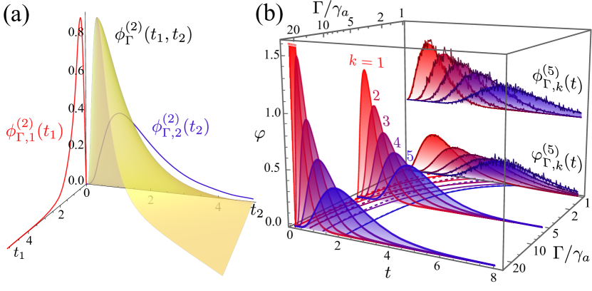
Figure 1: Filtered $N$-photon spontaneous emission. (a) For $N=2$ photons, one can visualize the full pdf $\phi^{(2)}_{\Gamma}(t_{1},t_{2})=2\gamma_{a}^{2}(\Gamma/\Gamma_{-})^{4}g^{\prime}(t_{1})g^{\prime}(t_{2})\mathbf{1}_{[t_{1},\infty[}(t_{2})$ in addition to its marginals $\phi_{\Gamma,k}^{(2)}(t_{k})$ which are its projections on the single-photon subspaces. (b) Marginals for $N=5$ for various filter widths $\Gamma$, conditioned ($\phi$, up) or not ($\varphi$, down) to full-bundle detection. The case $\Gamma/\gamma_{a}=1$ has superimposed a numerical simulation. On the floor, the mean times (5) showing dilation of the bundles under filtering (solid for $\varphi$, dashed for $\phi$).

This generalizes the unfiltered-photons result $\lim_{\Gamma\to\infty}\langle t_{k}^{(N)}\rangle=(H_{N}-H_{N-k})/\gamma_{a}$ (with $H_{N}$ the $N$th harmonic number and assuming $H_{0}\equiv 0$) and explains the observed photon-bundle time length (the time between the first and last detected photons) $\langle\tau\rangle_{N}\equiv\langle t_{N}^{(N)}\rangle-\langle t_{1}^{(N)}\rangle$ that goes to $H_{N-1}/\gamma_{a}$ in this limit, as was observed in Refs. sanchezmunoz14a ; arXiv_cosacchi21a , as well as the $k$th photon lifetime measured as $\langle t_{k}^{(N)}\rangle-\langle t_{k-1}^{(N)}\rangle\to 1/(\gamma_{a}k)$ as was observed in Refs. wang08b ; brune08a . Now in possession of the full probability distribution, we can also derive statistical quantities previously out of reach even in the limit $\Gamma\to\infty$, such as the standard deviation $\sigma_{\Gamma,k}^{(N)}$ for the emission time of the $k$th photon from a $N$-photon bundle, $\gamma_{a}\sigma_{\infty,k}^{(N)}={\sqrt{H_{N,2}-H_{N-k,2}}}$ multisup with $H_{N,2}\equiv\sum_{k=1}^{N}{k^{-2}}$ (generalized harmonic numbers). In the opposite limit, the same harmonic structure is found but this time governed by the filter alone with no direct influence (to leading order) from the radiative decay, with, e.g., $\langle t_{k}^{(N)}\rangle\sim(H_{N}-H_{N-k})/\Gamma$ as $\Gamma\to 0$, so:

$$\langle\tau\rangle_{N}={H_{N-1}\over\Gamma}\text{ at small~{}$\Gamma$}\text{ and }{H_{N-1}\over\gamma_{a}}\text{ at large~{}$\Gamma$}\,.$$ (6)

To unify these two simple and symmetric limits, one has to use Eq. (5). This time-dilation of a filtered bundle is shown on the floor of Fig. 1(b). We now turn to a richer, more accessible and more insightful statistical quantity that will further allow us to generalize our discussion to other types of multiphoton emission, namely, the waiting-time distribution (wtd), i.e., the probability distribution of the time difference between successive photons. For the SE of a two-photon bundle, this is obtained from Eq. (4) as $w_{2}(\tau)=\int_{0}^{\infty}\phi^{(2)}_{\Gamma}(t,\tau+t)\,dt$, which gives $w_{2}(\tau)={\Gamma\gamma_{a}(\Gamma+\gamma)\over(\Gamma-\gamma_{a})^{2}(3\Gamma+\gamma)(\Gamma+3\gamma_{a})}(\Gamma(3\Gamma+\gamma_{a})e^{-\gamma_{a}\tau}+\gamma_{a}(\Gamma+3\gamma_{a})e^{-\Gamma\tau}-8\Gamma\gamma_{a}e^{-{\Gamma+\gamma_{a}\over 2}\tau})$. This is a tri-exponential decay that balances the radiative decay with its filtering. This quantity provides another way to the average time length of a two-photon bundle as a function of filtering $\langle\tau\rangle_{2}=\int_{0}^{\infty}\tau w_{2}(\tau)d\tau={1\over\Gamma}+{1\over\gamma_{a}}+{2\over\gamma_{a}+\Gamma}-{9\over 4(3\Gamma+\gamma_{a})}-{9\over 4(\Gamma+3\gamma_{a})}$ (this is, alternatively, obtained from Eq. (5) as $\langle t_{2}^{(2)}\rangle-\langle t_{1}^{(2)}\rangle$), which recovers the limits (6) with numerator $H_{2}=1$.

This completes our description of filtered SE of Fock states, which is the starting point and reference for all other types of multiphoton emission, for instance, steady-state $N$-photon emission. We focus for now on the simplest case $N=2$. We simulate numerically with a frequency-resolved Monte Carlo method lopezcarreno18a a filtered “bundler” (emitter of bundles) sanchezmunoz14a , i.e., a coherently driven Jaynes-Cummings Hamiltonian in the dispersive limit, that can also be understood as a Purcell-enhanced Mollow-triplet. We compare both its wtd and its photon-purity $\pi_{2}$ (the percentage of unbroken bundles or photons emitted in pairs) with a toy-model of CWSE (continuous wave spontaneous emission) that simulates the actual emission of the bundler with randomly triggered SE of two-photon Fock states. For the most part, we find that the multiphoton emission from the bundler behaves accordingly to the SE of collapsed Fock states, as has been suggested all along strekalov14a . Their wtd, shown in Fig. 2(a) for different purities (50% and 100%), share the same qualitative main features. The multiphoton peak, in particular, i.e., the short-time excess of probabilities due to photons piling up from the multiphotons, behaves similarly under filtering. This is shown in Fig. 2(b) where numerically simulated CWSE and two-photon bundling are superimposed on the theoretical $\langle\tau\rangle_{2}$ above. There are, nevertheless, noteworthy quantitative departures, most prominently, the greater robustness of the bundles to filtering, as seen in Fig. 2(c) where the purity corresponds to that of SE with an effective decay rate of $\approx\gamma_{a}/2$. Therefore, for the same filter width, bundles originating from the driven system (bundler) are significantly more likely to be fully detected than if they were emitted by SE. This is surprising given the otherwise excellent agreement with a picture of collapsed Fock states that are subsequently spontaneously emitted. One can track this departure to the dynamics of the emitter itself (the two-level system) that, upon collapsing, resets the SE process in a mechanism akin to the quantum Zeno effect misra77a that effectively slows down the emission, i.e., reduces $\gamma_{a}$. This, in turn, makes the multiphoton detection more robust, since filtered SE is indeed better for larger $\Gamma/\gamma_{a}$. This dynamical enhancement depends on various parameters such as the statistics of the bundles themselves, which warrants a study on its own. This suggests, however, that the prospects of improving multiphoton emission by frequency filtering are even better than has been anticipated sanchezmunoz18a .

Finally, one cannot address multiphoton emission without considering the most famous and pervading case, which has been foundational to quantum optics hanburybrown56b and whose role remains central for applications valencia05a , let alone this being the most common type of light, namely, the thermal state. This is obtained by supplementing the Lindblad master equation of SE with a pumping term $\frac{P_{a}}{2}(2{a^{\dagger}}\rho{a}-a{a^{\dagger}}\rho-\rho a{a^{\dagger}})$ where $P_{a}<\gamma_{a}$ drives the cavity to a steady state $\rho=(1-\theta)\sum_{n=0}^{\infty}\theta^{n}\left|n\right\rangle\left\langle n\right|$ with effective temperature $\theta\equiv{P_{a}/\gamma_{a}}$. We can now precise its perceived relationship to multiphoton emission by comparing thermal light to pure multiphoton emission. The Laplace transform of the wtd is obtained from the same transform $\tilde{g}^{(2)}(s)$ of the $g^{(2)}(\tau)$ function kim87a as $\tilde{w}_{\mathrm{th}}(s)=(1+1/[\gamma_{a}n_{a}\tilde{g}^{(2)}(s)])^{-1}$ or, by inverse transform, $w_{\mathrm{th}}(\tau)=\frac{2P_{a}\gamma_{a}Q_{a}^{-1}}{\gamma_{a}-P_{a}}\exp{\big{[}\frac{-(\gamma_{a}^{2}+P_{a}^{2})\tau}{2(\gamma_{a}-P_{a})}\big{]}}\big{\{}Q_{a}\cosh\big{[}\frac{Q_{a}\tau}{2(\gamma_{a}-P_{a})}\big{]}\!-\!2P_{a}\gamma_{a}\sinh\big{[}\frac{Q_{a}\tau}{2(\gamma_{a}-P_{a})}\big{]}\big{\}}$, where we have defined $Q_{a}^{2}\equiv P_{a}^{4}-4P_{a}^{3}\gamma_{a}+10P_{a}^{2}\gamma_{a}^{2}-4P_{a}\gamma_{a}^{3}+\gamma_{a}^{4}$. This has a similar shape (cf. Fig. 2(a), green dotted line) than the wtd of the multiphoton emissions previously described, but behaves distinctively under filtering. For instance, let us compare the average of the thermal multiphoton peak $\langle\tau_{\Gamma}\rangle_{\mathrm{th}}$ with its pure multiphoton counterpart in Eq. (6): in the limit of large-bandwidth filtering, the average is that of a thermal state, $\langle\tau_{\infty}\rangle_{\mathrm{th}}=(\gamma_{a}-P_{a})/(P_{a}^{2}+\gamma_{a}^{2}+Q_{a})$, shown in the inset of Fig. 2(b). It is, in units of $\gamma_{a}$, a quantity between 0 (when $P_{a}\to\gamma_{a}$ with the multiphoton peak becoming a Dirac $\delta$ function) and $1$ (when $P_{a}\to 0$ with the multiphoton peak reducing to two-photon bunching and thus to the radiative lifetime). It is thus continuous, in contrast to pure multiphoton emission that is quantized (through the Harmonic numbers). For finite $\Gamma$, the average is not that of a thermal state anymore, since, surprisingly, although filtering has a tendency to thermalize quantum states, and does this exactly in the limit $\Gamma\to 0$ for all physical states, filtering a thermal state does not produce another thermal state, despite the fact that all the Glaubler correlators of the filtered thermal field $g^{(n)}_{\Gamma}(0)=n!$ remain the same. Their time dynamics, however, exhibit a different evolution multisup . Since in the limit $\Gamma\to 0$, a thermal state is again recovered as a universal limit, one can obtain the asymptotic behaviour: $\gamma_{a}\langle\tau_{0}\rangle_{\mathrm{th}}=\langle\tau_{\infty}\rangle_{\mathrm{th}}(1-\theta)/\Gamma$. Filtering pure multiphoton emission, on the other hand, produces bundles of various sizes, which yields a multiphoton peak in the wtd $\langle\tilde{\tau}\rangle_{N}\equiv{\sum_{k=2}^{N}{\langle t_{k}^{(N)}\rangle-\langle t_{1}^{(N)}\rangle\over k-1}P(k,N)/\sum_{k=2}^{N}P(k,N)}$ obtained by weighting the contribution of each sub-bundle population. This is qualitatively different from thermal emission, that retains thermal contributions from multiphotons of all sizes. Therefore, even if the wide-filter asymptotes $\langle\tau_{\infty}\rangle_{\mathrm{th}}$ and $\langle\tilde{\tau}\rangle_{N}$ match, their narrow-filter trends depart as shown in Fig. 2(b). This disconnection of the two limits, as compared to Eq. (6), shows that there are dynamical features present in thermal equilibrium that break from the paradigm of SE. In the limit $\Gamma\to 0$, another unexpected result is found: the thermal field is monochromatic though chaotic, as was already understood by Glauber glauber63a . The surprise is that its temperature $\theta_{\mathrm{th},\Gamma}=P_{a}\gamma_{a}/(P_{a}^{2}+(\gamma_{a}+\Gamma)(\gamma_{a}-P_{a}))$, as compared to that of the unfiltered field $\theta_{\mathrm{th}}=P_{a}/\gamma_{a}$, can be higher (if $\Gamma<P_{a}$), although one is only interposing a passive element. This apparent paradox is due to both fields having different time scales, with the filter slowing down times by delaying photons. As a result, the filtered photons can have a flatter distribution of photon-numbers, with higher probabilities to find more excited-states, but these also have a longer lifetime, so are less likely to be emitted, thus conserving energy while increasing temperature. This could also be seen as a CW version of an equally surprising phenomenon when subtracting a single photon from a thermal field, that results in increasing its average population parigi07a . These various findings in multiphoton emission provide insightful relationships and departures between a thermal state and pure multiphoton sources. Their closest encounter is at vanishing temperature where a thermal state then behaves as a two-photon source but with most of its bundles broken… A fairly subtle and elusive connection!

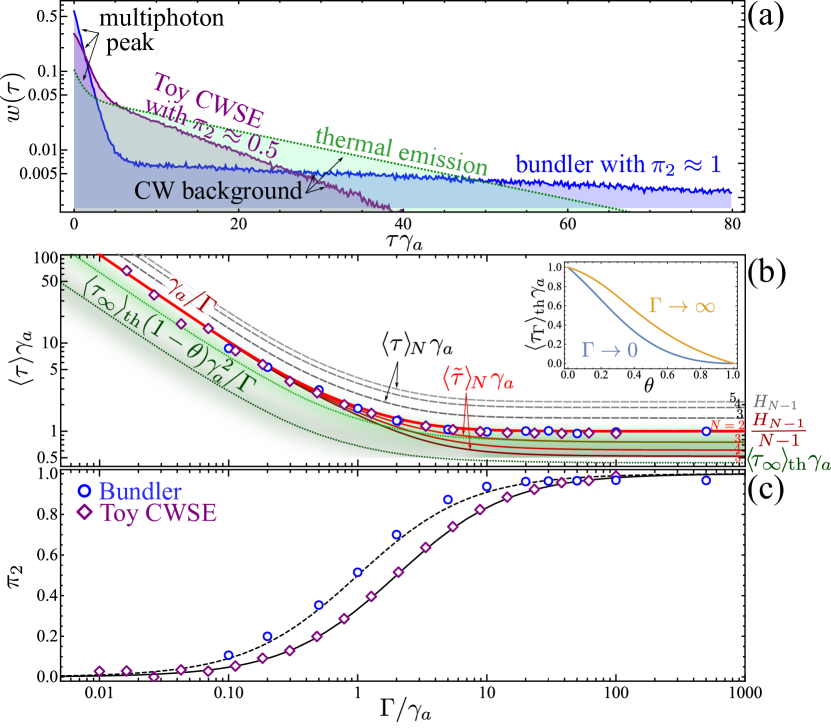
Figure 2: Dynamical multiphoton emission. (a) wtd for the toy-model (CWSE of Fock states, purple), the bundler (blue) and a thermal state (dotted green), all featuring a multiphoton peak sitting on the background of successive multiphotons. The toy model and bundler would be identical if they had the same purity. (b) Multiphoton peak average as a function of filtering, for the case of pure multiphoton emission $\langle\tilde{\tau}\rangle_{N}$ for $N$ from 2 to 5, exhibiting quantization at large $\Gamma$ and a unique asymptote at small $\Gamma$ when all bundles are broken into two-photon ones. The toy-model (purple diamonds) and the bundler (blue circles) behave according to the SE picture (red thick line). In contrast, the filtered thermal multiphoton-peak averages $\langle\tau_{\Gamma}\rangle_{\mathrm{th}}$ are not quantized (shading) and retain multiphoton contributions to all orders. In inset, average of the thermal multiphoton peak in its wtd as a function of $\theta\equiv P_{a}/\gamma_{a}$ leading to different asymptotes. Dashed gray lines: $N$-photon bundle time length $\langle\tau\rangle_{N}$ also featuring same coefficients for the asymptotes. (c) Two-photon purity [percentage of fully detected bundles] from Fock state SE (line), the toy-model (diamonds) and the bundler (circles) which higher purity fits well with a SE rate of $\approx\gamma_{a}/2$ (dotted lines).

In conclusion, we have provided a comprehensive and analytical description of the fundamental case of SE of Fock states, illustrated with statistical observables of interest. The treatment through frequency filtering allows to describe at a fundamental level the detection process. While we have focused on time observables, the same analysis could be done in the frequency domain by Fourier transform of Eq. (4), providing probabilities of detections at given frequencies. Compared to other types of multiphoton emission, we have shown that although a bundler behaves in all respect as SE of collapsed Fock states, dynamical features exist that protect bundles, making them significantly more resilient to filtering than if they were generated by SE. This calls for further studies to understand, characterize and exploit such dynamical advantages. We have also highlighted connections and departures with thermal light, which features multiphoton emission to all orders of a different character than pure multiphoton emission with broken bundles. Such characterizations could also be made for superchaotic light, superbunching, leapfrog processes in resonance fluorescence, etc., which should enlighten on the nature, character and relationship of these sources with pure multiphoton emission, thus allowing to establish a zoology of its various types.

- (1) Deléglise, S. et al. Reconstruction of non-classical cavity field states with snapshots of their decoherence. Nature 455, 510 (2008). http://doi.org/10.1038/nature07288.
- (2) Hofheinz, M. et al. Generation of Fock states in a superconducting quantum circuit. Nature 454, 310 (2008). http://doi.org/10.1038/nature07136.
- (3) Sayrin, C. et al. Real-time quantum feedback prepares and stabilizes photon number states. Nature 477, 73 (2011). http://doi.org/10.1038/nature10376.
- (4) Chu, Y. et al. Creation and control of multi-phonon Fock states in a bulk acoustic-wave resonator. Nature 563, 666 (2018). http://doi.org/10.1038/s41586-018-0717-7.
- (5) Sánchez Muñoz, C. & Schlawin, F. Photon correlation spectroscopy as a witness for quantum coherence. Phys. Rev. Lett. 124, 203601 (2020). http://doi.org/10.1103/PhysRevLett.124.203601.
- (6) Viñas Boström, E., D’Andrea, A., Cini, M. & Verdozzi, C. Time-resolved multiphoton effects in the fluorescence spectra of two-level systems at rest and in motion. Phys. Rev. A 102, 103719 (2020). http://doi.org/10.1103/PhysRevA.102.013719.
- (7) Zhong, H.-S. et al. Quantum computational advantage using photons. Science 370, 1460 (2020). http://doi.org/10.1126/science.abe8770.
- (8) Uria, M., Solano, P. & Hermann-Avigliano, C. Deterministic generation of large fock states. Phys. Rev. Lett. 125, 093603 (2020). http://doi.org/10.1103/PhysRevLett.125.093603.
- (9) Mandel, L. Fluctuations of photon beams: The distribution of the photo-electrons. Proc. Roy. Soc 74, 233 (1959). http://doi.org/10.1088/0370-1328/74/3/301.
- (10) Kelley, P. L. & Kleiner, W. H. Theory of electromagnetic field measurement and photoelectron counting. Phys. Rev. 136, A316 (1964). http://doi.org/10.1103/PhysRev.136.A316.
- (11) Glauber, R. J. Photon correlations. Phys. Rev. Lett. 10, 84 (1963). http://doi.org/10.1103/PhysRevLett.10.84.
- (12) Sánchez Muñoz, C. et al. Emitters of -photon bundles. Nature Photon. 8, 550 (2014). http://doi.org/10.1038/nphoton.2014.114.
- (13) Dong, X.-L. & Li, P.-B. Multiphonon interactions between nitrogen-vacancy centers and nanomechanical resonators. Phys. Rev. A 100, 043825 (2019). http://doi.org/10.1103/PhysRevA.100.043825.
- (14) Bin, Q., Lü, X.-Y., Laussy, F. P., Nori, F. & Wu, Y. -phonon bundle emission via the stokes process. Phys. Rev. Lett. 124, 053601 (2020). http://doi.org/10.1103/PhysRevLett.124.053601.
- (15) Q. Bin, Y. W. & Lü, X.-Y. Parity-symmetry-protected multiphoton bundle emission. Phys. Rev. Lett. 127, 073602 (2021). http://doi.org/10.1103/PhysRevLett.127.073602.
- (16) Ma, S., Li, X., Ren, Y., Xie, J. & Li, F. Antibunched -photon bundles emitted by a josephson photonic device. Phys. Rev. Res. 3, 043020 (2021). http://doi.org/10.1103/PhysRevResearch.3.043020.
- (17) Deng, Y., Shi, T. & Yi, S. Motional -phonon bundle states of a trapped atom with clock transitions. Phot. Res. 9, 1289 (2021). http://doi.org/10.1364/PRJ.427062.
- (18) Cosacchi, M. et al. Suitability of solid-state platforms as sources of -photon bundles. arXiv:2108.03967 (2021).
- (19) Scully, M. O. & W. E. Lamb, J. Quantum theory of an optical maser. III. Theory of photoelectron counting statistics. Phys. Rev. 179, 368 (1969). http://doi.org/10.1103/PhysRev.179.368.
- (20) Arnoldus, H. F. & Nienhuis, G. Photon correlations between the lines in the spectrum of resonance fluorescence. J. Phys. B.: At. Mol. Phys. 17, 963 (1984). http://doi.org/10.1088/0022-3700/17/6/011.
- (21) Eberly, J. & Wódkiewicz, K. The time-dependent physical spectrum of light. J. Opt. Soc. Am. 67, 1252 (1977). http://doi.org/10.1364/JOSA.67.001252. TDS1.3.
- (22) del Valle, E., González-Tudela, A., Laussy, F. P., Tejedor, C. & Hartmann, M. J. Theory of frequency-filtered and time-resolved -photon correlations. Phys. Rev. Lett. 109, 183601 (2012). http://doi.org/10.1103/PhysRevLett.109.183601.
- (23) Díaz Camacho, G. et al. Supplementary material. (online) (2021).
- (24) Wang, H. et al. Measurement of the decay of Fock states in a superconducting quantum circuit. Phys. Rev. Lett. 101, 240401 (2008). http://doi.org/10.1103/PhysRevLett.101.240401.
- (25) Brune, M. et al. Process tomography of field damping and measurement of Fock state lifetimes by quantum nondemolition photon counting in a cavity. Phys. Rev. Lett. 101, 240402 (2008). http://doi.org/10.1103/PhysRevLett.101.240402.
- (26) López Carreño, J. C., del Valle, E. & Laussy, F. P. Frequency-resolved Monte Carlo. Sci. Rep. 8, 6975 (2018). http://doi.org/10.1038/s41598-018-24975-y.
- (27) Strekalov, D. V. Cavity quantum electrodynamics: A bundle of photons, please. Nature Photon. 8, 500 (2014). http://doi.org/10.1038/nphoton.2014.144.
- (28) Misra, B. & Sudarshan, E. C. G. The Zeno’s paradox in quantum theory. J. Math. Phys. 18, 756 (1977). http://doi.org/10.1063/1.523304.
- (29) Sánchez Muñoz, C., Laussy, F. P., del Valle, E., Tejedor, C. & González-Tudela, A. Filtering multiphoton emission from state-of-the-art cavity QED. Optica 5, 14 (2018). http://doi.org/10.1364/OPTICA.5.000014.
- (30) Hanbury Brown, R. & Twiss, R. Q. Correlation between photons in two coherent beams of light. Nature 177, 27 (1956). http://doi.org/10.1038/177027a0.
- (31) Valencia, A., Scarcelli, G., D’Angelo, M. & Shih, Y. Two-photon imaging with thermal light. Phys. Rev. Lett. 94, 063601 (2005). http://doi.org/10.1103/PhysRevLett.94.063601.
- (32) Kim, M., Knight, P. & Wodkjewicz, K. Correlations between successively emitted photons in resonance fluorescence. Opt. Commun. 62, 385 (1987). http://doi.org/10.1016/0030-4018(87)90005-8.
- (33) Parigi, V., Zavatta, A., Kim, M. & Bellini, M. Probing quantum commutation rules by addition and subtraction of single photons to/from a light field. Science 317, 1890 (2007). http://doi.org/10.1126/science.1146204.