Anomalous diffusion in QCD matter

Paul Caucal pcaucal@bnl.gov Physics Department, Brookhaven National Laboratory, Upton, NY 11973, USA โ€ƒโ€ƒ Yacine Mehtar-Tani mehtartani@bnl.gov Physics Department, Brookhaven National Laboratory, Upton, NY 11973, USA RIKEN BNL Research Center, Brookhaven National Laboratory, Upton, NY 11973, USA
Abstract

We study the effects of quantum corrections on transverse momentum broadening of a fast parton passing through dense QCD matter. We show that, at leading logarithmic accuracy the broadening distribution tends at late times or equivalently for large system sizes $L$ to a universal distribution that only depends on a single scaling variable kโŸ‚2/Qs2subscriptsuperscript๐‘˜2perpendicular-tosubscriptsuperscript๐‘„2๐‘ k^{2}_{\perp}/Q^{2}_{s} where the typical transverse momentum scale increases with time as lnโกQs2โ‰ƒ(1+2โ€‹ฮฒ)โ€‹lnโกLโˆ’32โ€‹(1+ฮฒ)โ€‹lnโกlnโกLsimilar-to-or-equalssuperscriptsubscript๐‘„๐‘ 212๐›ฝ๐ฟ321๐›ฝ๐ฟ\ln Q_{s}^{2}\simeq(1+2\beta)\ln L-\frac{3}{2}(1+\beta)\,\ln\ln L up to non-universal terms, with an anomalous dimension ฮฒโˆผฮฑssimilar-to๐›ฝsubscript๐›ผ๐‘ \beta\sim\sqrt{\alpha_{s}}. This property is analogous to geometric scaling of gluon distributions in the saturation regime and traveling waves solutions to reaction-diffusion processes. We note that since $\beta>0$ the process is super-diffusive, which is also reflected at large transverse momentum where the scaling distribution exhibits a heavy tail $k_{\perp}^{4-2\beta}$ akin to Lรฉvy random walks.

Transverse momentum broadening (TMB) of energetic quarks and gluons while traversing QCD matter plays a central role in a variety of processes studied at colliders to probe QCD, ranging from jet suppression in heavy ion collisions Blaizotย andย Mehtar-Tani (2015); Qinย andย Wang (2015) to transverse momentum dependent gluon distribution function that encode information on the 3D structure of the proton and nuclei in high energy collisions in particular at small Bjorken $x$ where gluon saturation is expected to take place Lipatov (1997); Gelisย etย al. (2010); Albaceteย andย Marquet (2014).

High energy partons experience random kicks in hot or cold nuclear matter that cause their transverse momentum $\boldsymbol{k}_{\perp}$ w.r.t. to their direction of motion to increase over time. The leading order elastic process is given by a single gluon exchange via Coulomb scattering and leads to an approximate brownian motion in transverse momentum space, so long as the mean free path is larger than the in-medium correlation length, where the typical transverse momentum square scales linearly with system size $L$, namely $\langle k_{\perp}^{2}\rangle_{\rm typ}\sim\hat{q}\,L$, where $\hat{q}$ is the diffusion coefficient.

Moreover, radiative processes can also increase transverse momentum of the leading parton due to recoil effects. This question was recently addressed, and it has been shown that such contributions, albeit suppressed by the coupling constant ฮฑssubscript๐›ผ๐‘ \alpha_{s}, are enhanced by double logarithms which must be resummed to all orders when ฮฑsโ€‹ln2โกLโˆผ1similar-tosubscript๐›ผ๐‘ superscript2๐ฟ1\alpha_{s}\ln^{2}L\sim 1 Liouย etย al. (2013); Blaizotย etย al. (2014); Blaizotย andย Mehtar-Tani (2014); Iancu (2014).

In this letter we go beyond this result by investigating in more detail the consequences of the non-local nature of the quantum corrections on the TMB distribution. We find in particular that the latter reaches a universal scaling solution at late times (large $L$) that we compute analytically along with its sub-asymptotic deviations exploiting a formal analogy between the present problem and traveling wave solutions to reaction-diffusion processes Munierย andย Peschanski (2003). As a consequence of the self-similarity characterizing the anomalous random walk, the TMB distribution is of Lรฉvy type. It is in particular associated with a heavy power law tail describing long rare steps which extends over a large range of transverse momenta above the typical transverse momentum scale.

Lรฉvy flights are ubiquitous in nature and span a wide variety of stochastic processes in biological systems Viswanathanย etย al. (1996); Edwardsย etย al. (2007), molecular chemistry Zumofenย andย Klafter (1994), optical lattice Katoriย etย al. (1997), turbulent diffusion and polymer transport theory Shlesingerย etย al. (1993, 1995). Furthemore, heavy tailed distributions are also observed in self-organized critical states Bakย etย al. (1987, 1988). In this work, we point out for the first time another occurrence of such random walks in the transport of eikonal partons in dense QCD matter and we compute the anomalous exponents that characterize the deviation to standard diffusion.

I Quantum corrections to transverse momentum broadening in QCD media

The TMB distribution is related to the forward scattering amplitude $\mathcal{S}(\boldsymbol{x}_{\perp})$ of an effective dipole in color representation $R=A,F$ with transverse size $\boldsymbol{x}_{\perp}$(see e.g. Blaizotย etย al. (2014); Kovchegovย andย Levin (2012); Dโ€™Eramoย etย al. (2011)) via a Fourier transform,

$$\mathcal{P}(\boldsymbol{k}_{\perp})=\int{\rm d}^{2}\boldsymbol{x}_{\perp}{\rm e}^{-i\boldsymbol{k}_{\perp}\cdot\boldsymbol{x}_{\perp}}\mathcal{S}(\boldsymbol{x}_{\perp})\,.$$ (1)

Considering the dipole formulation in position space allows for a straightforward resummation of multiple scattering by exponentiating the single scattering cross-section, so long as the interactions between the dipole and the medium are local and instantaneous. Thus, we may write $\mathcal{S}(\boldsymbol{x}_{\perp})=\exp(-\frac{1}{4}\frac{C_{R}}{N_{c}}\,\hat{q}(1/\boldsymbol{x}_{\perp}^{2})L\,\boldsymbol{x}_{\perp}^{2})$ 111We use bold type for two dimensional transverse vectors and note $a_{T}=|\boldsymbol{a}_{\perp}|$.. The latter relation defines the quenching parameter in the adjoint representation which is assumed to be a slowly varying function of $\boldsymbol{x}_{\perp}$. At tree-level it reads

$$\hat{q}^{(0)}(1/\boldsymbol{x}_{\perp}^{2})=\hat{q}_{0}\ln\left(\frac{1}{\boldsymbol{x}_{\perp}^{2}\mu^{2}}\right)\,,$$ (2)

up to powers of $x_{T}\mu$ suppressed terms. For a weakly coupled QGP the bare quenching parameter $\hat{q}_{0}$ and the infrared transverse scale $\mu^{2}$ 222$\mu^{2}$ can be obtained from the hard thermal loop value of the collision rate Aurencheย etย al. (2002). They read respectively q^0=ฮฑsโ€‹Ncโ€‹mD2โ€‹Tsubscript^๐‘ž0subscript๐›ผ๐‘ subscript๐‘๐‘superscriptsubscript๐‘š๐ท2๐‘‡\hat{q}_{0}=\alpha_{s}N_{c}m_{D}^{2}T and $\mu=m_{D}{\rm e}^{-1+\gamma_{E}}/2$ Barataย etย al. (2020), with $T$ the plasma temperature, $m_{D}$ the Debye mass. are related to the Debye screening mass in the QGP or to the inverse nucleon size in a nucleus.

It is customary to define the emergent saturation scale Qsโ€‹(L)subscript๐‘„๐‘ ๐ฟQ_{s}(L) via the relation ๐’ฎโ€‹(๐’™โŸ‚2=1/Qs2โ€‹(L))โ‰กeโˆ’1/4๐’ฎsuperscriptsubscript๐’™perpendicular-to21superscriptsubscript๐‘„๐‘ 2๐ฟsuperscripte14\mathcal{S}(\boldsymbol{x}_{\perp}^{2}=1/Q_{s}^{2}(L))\equiv\mathrm{e}^{-1/4}, or equivalently, q^โ€‹(Qs2โ€‹(L))โ€‹Lโ‰กQs2โ€‹(L)^๐‘žsuperscriptsubscript๐‘„๐‘ 2๐ฟ๐ฟsuperscriptsubscript๐‘„๐‘ 2๐ฟ\hat{q}(Q_{s}^{2}(L))L\equiv Q_{s}^{2}(L). This definition is standard in small-$x$ physics Kowalskiย andย Teaney (2003); Lappi (2011), and is also motivated by Moliรจre theory of multiple scattering Moliere (1948); Bethe (1953); Barataย etย al. (2020) in which Qssubscript๐‘„๐‘ Q_{s} is the transverse scale that controls the transition between the multiple soft scattering and the single hard scattering regimes. Given Eq.โ€‰(2), one finds Qs2โˆผq^0โ€‹Lโ€‹lnโก(q^0โ€‹L/ฮผ2)similar-tosuperscriptsubscript๐‘„๐‘ 2subscript^๐‘ž0๐ฟsubscript^๐‘ž0๐ฟsuperscript๐œ‡2Q_{s}^{2}\sim\hat{q}_{0}L\ln(\hat{q}_{0}L/\mu^{2}) at tree level.

Beyond leading order in ฮฑssubscript๐›ผ๐‘ \alpha_{s}, one has to account for real and virtual gluon fluctuations in the effective dipole with lifetime $\tau$ smaller than the system size. Such fluctuations yield potentially large contributions of the form q^(1)โˆผฮฑsโ€‹q^(0)โ€‹ln2โก(L/ฯ„0)similar-tosuperscript^๐‘ž1subscript๐›ผ๐‘ superscript^๐‘ž0superscript2๐ฟsubscript๐œ0\hat{q}^{(1)}\sim\alpha_{s}\hat{q}^{(0)}\ln^{2}(L/\tau_{0}) with $\tau_{0}\ll L$ a microscopic scale of order of the mean free path Liouย etย al. (2013). These radiative corrections to the quenching parameter can be resummed to double logarithmic accuracy (DLA) via an evolution equation ordered in $\tau$ย Liouย etย al. (2013); Blaizotย andย Mehtar-Tani (2014); Iancu (2014):

$\displaystyle\hat{q}(\tau,\boldsymbol{k}_{\perp}^{2})$ =q^(0)+โˆซฯ„0ฯ„dโ€‹ฯ„โ€ฒฯ„โ€ฒโ€‹โˆซQs2โ€‹(ฯ„โ€ฒ)๐’ŒโŸ‚2dโ€‹๐’ŒโŸ‚โ€ฒโฃ2๐’ŒโŸ‚โ€ฒโฃ2โ€‹ฮฑยฏsโ€‹q^โ€‹(ฯ„โ€ฒ,๐’ŒโŸ‚โ€ฒโฃ2),absentsuperscript^๐‘ž0superscriptsubscriptsubscript๐œ0๐œdsuperscript๐œโ€ฒsuperscript๐œโ€ฒsuperscriptsubscriptsubscriptsuperscript๐‘„2๐‘ superscript๐œโ€ฒsuperscriptsubscript๐’Œperpendicular-to2dsuperscriptsubscript๐’Œperpendicular-toโ€ฒ2superscriptsubscript๐’Œperpendicular-toโ€ฒ2subscriptยฏ๐›ผ๐‘ ^๐‘žsuperscript๐œโ€ฒsuperscriptsubscript๐’Œperpendicular-toโ€ฒ2\displaystyle=\hat{q}^{(0)}+\int_{\tau_{0}}^{\tau}\frac{{\rm d}\tau^{\prime}}{\tau^{\prime}}\int_{Q^{2}_{s}(\tau^{\prime})}^{\boldsymbol{k}_{\perp}^{2}}\frac{{\rm d}\boldsymbol{k}_{\perp}^{\prime 2}}{\boldsymbol{k}_{\perp}^{\prime 2}}\ \bar{\alpha}_{s}\ \hat{q}(\tau^{\prime},\boldsymbol{k}_{\perp}^{\prime 2})\,, (3)
Qs2โ€‹(ฯ„)subscriptsuperscript๐‘„2๐‘ ๐œ\displaystyle Q^{2}_{s}(\tau) =q^โ€‹(ฯ„,Qs2โ€‹(ฯ„))โ€‹ฯ„,absent^๐‘ž๐œsuperscriptsubscript๐‘„๐‘ 2๐œ๐œ\displaystyle=\hat{q}(\tau,Q_{s}^{2}(\tau))\tau\,, (4)

where ฮฑยฏs=ฮฑsโ€‹Nc/ฯ€subscriptยฏ๐›ผ๐‘ subscript๐›ผ๐‘ subscript๐‘๐‘๐œ‹\bar{\alpha}_{s}=\alpha_{s}N_{c}/\pi and $\hat{q}^{(0)}\equiv\hat{q}(\tau_{0},\boldsymbol{k}_{\perp})$ . The condition ๐’ŒโŸ‚2โ‰ฅQs2โ€‹(ฯ„)superscriptsubscript๐’Œperpendicular-to2subscriptsuperscript๐‘„2๐‘ ๐œ\boldsymbol{k}_{\perp}^{2}\geq Q^{2}_{s}(\tau) in Eq.โ€‰(3) enforces the gluon fluctuations to be triggered by a single scattering with plasma constituents whose contribution is logarithmically enhanced compared to multiple scattering. The final value of $\tau$ is fixed at the largest time allowed by the saturation condition, i.e.ย at the time scale $\tau$ such that Qs2โ€‹(ฯ„)=๐’ŒโŸ‚2superscriptsubscript๐‘„๐‘ 2๐œsuperscriptsubscript๐’Œperpendicular-to2Q_{s}^{2}(\tau)=\boldsymbol{k}_{\perp}^{2}, as long as $\tau<L$ and $\tau=L$ otherwise. The latter case corresponds to the dilute regime Blaizotย andย Dominguez (2019), that is when ๐’ŒโŸ‚2โ‰ซQs2โ€‹(L)much-greater-thansuperscriptsubscript๐’Œperpendicular-to2superscriptsubscript๐‘„๐‘ 2๐ฟ\boldsymbol{k}_{\perp}^{2}\gg Q_{s}^{2}(L).

In this letter, we address both analytically and numerically the non-linear system (3)-(4) 333See Supplemental Material 1 for detailed explanations about the numerical resolution of this non-linear differential system.. Analytic solutions are in general difficult to obtain, however, a solution for the linearized problem that consists in approximating Qs2โ€‹(ฯ„)โ‰ƒq^0โ€‹ฯ„similar-to-or-equalssuperscriptsubscript๐‘„๐‘ 2๐œsubscript^๐‘ž0๐œQ_{s}^{2}(\tau)\simeq\hat{q}_{0}\tau for the emission phase space can be found Iancuย andย Triantafyllopoulos (2014); Muellerย etย al. (2017). For a constant initial condition it reads

$\displaystyle\hat{q}(Y,\rho)$ =q^0โ€‹[I0โ€‹(2โ€‹ฮฑยฏsโ€‹Yโ€‹ฯ)โˆ’Yฯโ€‹I2โ€‹(2โ€‹ฮฑยฏsโ€‹Yโ€‹ฯ)],absentsubscript^๐‘ž0delimited-[]subscriptI02subscriptยฏ๐›ผ๐‘ ๐‘Œ๐œŒ๐‘Œ๐œŒsubscriptI22subscriptยฏ๐›ผ๐‘ ๐‘Œ๐œŒ\displaystyle=\hat{q}_{0}\left[\textrm{I}_{0}\left(2\sqrt{\bar{\alpha}_{s}Y\rho}\right)-\frac{Y}{\rho}\textrm{I}_{2}\left(2\sqrt{\bar{\alpha}_{s}Y\rho}\right)\right]\,, (5)

with $Y=\ln(\tau/\tau_{0})$ and $\rho=\ln(\boldsymbol{k}_{\perp}^{2}/(\hat{q}_{0}\tau_{0}))$ 444We note $\mathrm{I}_{n}$ the modified Bessel function of rank $n$. Formally, this linearization is valid in DLA, which captures all the terms of the form ฮฑยฏsnโ€‹Y2โ€‹nsuperscriptsubscriptยฏ๐›ผ๐‘ ๐‘›superscript๐‘Œ2๐‘›\bar{\alpha}_{s}^{n}Y^{2n} assuming $Y\sim\rho$, but it misses sub-leading corrections of the form ฮฑยฏsnโ€‹Y2โ€‹nโˆ’1โ€‹lnโกYsuperscriptsubscriptยฏ๐›ผ๐‘ ๐‘›superscript๐‘Œ2๐‘›1๐‘Œ\bar{\alpha}_{s}^{n}Y^{2n-1}\ln Y which are parametrically larger than the single logarithmic ones. This is one of the novelty of the present study, enabling us to highlight the geometric scaling property of the transverse momentum diffusion in QCD and to compute the scaling deviations.

II Geometric scaling and traveling waves

The TMB distribution is said to obey geometric scaling if it is only a function of ๐’ŒโŸ‚2/Qs2โ€‹(L)superscriptsubscript๐’Œperpendicular-to2subscriptsuperscript๐‘„2๐‘ ๐ฟ\boldsymbol{k}_{\perp}^{2}/Q^{2}_{s}(L) as a result of scaling invariance of the radiative process at late times. More precisely, we would have

limLโ†’โˆžq^โ€‹(๐’ŒโŸ‚2)โ€‹L=Qs2โ€‹(L)โ€‹fโ€‹(๐’ŒโŸ‚2Qs2โ€‹(L)),subscriptโ†’๐ฟ^๐‘žsuperscriptsubscript๐’Œperpendicular-to2๐ฟsuperscriptsubscript๐‘„๐‘ 2๐ฟ๐‘“superscriptsubscript๐’Œperpendicular-to2superscriptsubscript๐‘„๐‘ 2๐ฟ\lim\limits_{L\to\infty}\hat{q}(\boldsymbol{k}_{\perp}^{2})L=Q_{s}^{2}(L)f\left(\frac{\boldsymbol{k}_{\perp}^{2}}{Q_{s}^{2}(L)}\right)\,, (6)

for some scaling function $f$ to be determined. Note that the linearized version of Eq.โ€‰(3) satisfies a similar scaling relation with the notable difference that the argument of $f$ is $\boldsymbol{k}_{\perp}^{2}/(\hat{q}_{0}L)$ instead of ๐’ŒโŸ‚2/Qs2โ€‹(L)superscriptsubscript๐’Œperpendicular-to2superscriptsubscript๐‘„๐‘ 2๐ฟ\boldsymbol{k}_{\perp}^{2}/Q_{s}^{2}(L). The non-linearity of Eq.โ€‰(3) enforces the evolution to be controlled by a single momentum scale Qsโ€‹(L)subscript๐‘„๐‘ ๐ฟQ_{s}(L) 555Note that this property holds also for the tree level form of $\hat{q}$ as q^(0)โ€‹(๐’ŒโŸ‚2)โ€‹Lโ‰ƒQs2โ€‹(L)similar-to-or-equalssuperscript^๐‘ž0superscriptsubscript๐’Œperpendicular-to2๐ฟsuperscriptsubscript๐‘„๐‘ 2๐ฟ\hat{q}^{(0)}(\boldsymbol{k}_{\perp}^{2})L\simeq Q_{s}^{2}(L) for kTโ‰ชQs2โ€‹(L)/ฮผmuch-less-thansubscript๐‘˜๐‘‡superscriptsubscript๐‘„๐‘ 2๐ฟ๐œ‡k_{T}\ll Q_{s}^{2}(L)/\mu..

Geometric scaling was extensively studied in the context of deep inelastic scattering, where it has been shown that the gluon distribution $g(x,Q^{2})$ at small $x$ satisfies this property over a broad region of photon virtuality $-Q^{2}$ Stastoย etย al. (2001); Iancuย etย al. (2002); Kwiecinskiย andย Stasto (2002). We shall demonstrate that TMB exhibits similar properties.

Traveling waves (TW) solution.

Remarkably, it is possible to find the scaling function $f$ for the non-linear problem defined by Eqs.โ€‰(3)-(4). In terms of the variables $Y$ and $\rho$, the differential equation satisfied by $\hat{q}$ reads

โˆ‚q^โ€‹(Y,ฯ)โˆ‚Y=ฮฑยฏsโ€‹โˆซฯsโ€‹(Y)ฯdโ€‹ฯโ€ฒโ€‹q^โ€‹(Y,ฯโ€ฒ),^๐‘ž๐‘Œ๐œŒ๐‘Œsubscriptยฏ๐›ผ๐‘ superscriptsubscriptsubscript๐œŒ๐‘ ๐‘Œ๐œŒdsuperscript๐œŒโ€ฒ^๐‘ž๐‘Œsuperscript๐œŒโ€ฒ\frac{\partial\hat{q}(Y,\rho)}{\partial Y}=\bar{\alpha}_{s}\int_{\rho_{s}(Y)}^{\rho}\textrm{d}\rho^{\prime}\ \hat{q}(Y,\rho^{\prime})\,, (7)

with ฯs=lnโก(Qs2/(q^0โ€‹ฯ„0))subscript๐œŒ๐‘ superscriptsubscript๐‘„๐‘ 2subscript^๐‘ž0subscript๐œ0\rho_{s}=\ln(Q_{s}^{2}/(\hat{q}_{0}\tau_{0})). Let us now look for a scaling solution of the form q^โ€‹(Y,ฯ)=q^0โ€‹eฯsโ€‹(Y)โˆ’Yโ€‹fโ€‹(ฯโˆ’ฯsโ€‹(Y))^๐‘ž๐‘Œ๐œŒsubscript^๐‘ž0superscript๐‘’subscript๐œŒ๐‘ ๐‘Œ๐‘Œ๐‘“๐œŒsubscript๐œŒ๐‘ ๐‘Œ\hat{q}(Y,\rho)=\hat{q}_{0}e^{\rho_{s}(Y)-Y}f(\rho-\rho_{s}(Y)).

Plugging this expression in Eq.ย (7), one gets the following differential equation

โˆ’dโ€‹ฯsdโ€‹Yโ€‹fโ€ฒโ€ฒโ€‹(x)+[dโ€‹ฯsdโ€‹Yโˆ’1]โ€‹fโ€ฒโ€‹(x)โˆ’ฮฑยฏsโ€‹fโ€‹(x)=0,dsubscript๐œŒ๐‘ d๐‘Œsuperscript๐‘“โ€ฒโ€ฒ๐‘ฅdelimited-[]dsubscript๐œŒ๐‘ d๐‘Œ1superscript๐‘“โ€ฒ๐‘ฅsubscriptยฏ๐›ผ๐‘ ๐‘“๐‘ฅ0-\frac{\textrm{d}\rho_{s}}{\textrm{d}Y}f^{\prime\prime}(x)+\left[\frac{\textrm{d}\rho_{s}}{\textrm{d}Y}-1\right]f^{\prime}(x)-\bar{\alpha}_{s}f(x)=0\,, (8)

where x=ฯโˆ’ฯsโ€‹(Y)๐‘ฅ๐œŒsubscript๐œŒ๐‘ ๐‘Œx=\rho-\rho_{s}(Y). In order for $f$ to be a function of $x$ only at large $Y$, the derivative dโ€‹ฯs/dโ€‹Ydsubscript๐œŒ๐‘ d๐‘Œ\textrm{d}\rho_{s}/\textrm{d}Y must converge towards a constant $c$, which can be interpreted as the speed of a traveling wave that propagates to the right on the $\rho$ axis. This is reminiscent of the TW solutions Munierย andย Peschanski (2003) to the Balitsky-Kovchekov (BK) equation Balitsky (1996); Kovchegov (1999). The initial conditions to this second order linear differential equation follow from the non-linear treatment of the saturation boundary: on the isoline $x=0$, meaning ฯ=ฯsโ€‹(Y)๐œŒsubscript๐œŒ๐‘ ๐‘Œ\rho=\rho_{s}(Y), one has $f(0)=0$ and $f^{\prime}(0)=(c-1)/c$. It is then straightforward to solve Eq.ย (8) with the scaling form $f(x)\propto{\rm e}^{\beta x}$ where the slope $\beta$ is solution of the quadratic equation โˆ’cโ€‹ฮฒ2+(cโˆ’1)โ€‹ฮฒโˆ’ฮฑยฏs=0๐‘superscript๐›ฝ2๐‘1๐›ฝsubscriptยฏ๐›ผ๐‘ 0-c\beta^{2}+(c-1)\beta-\bar{\alpha}_{s}=0. For any initial condition such that $\hat{q}(Y=0,\rho)<{\rm e}^{\beta\rho}$ when $\rho\to\infty$ Brunetย andย Derrida (1997), which is the case in the present letter, the minimum value for $\beta$, that satisfies the additional constraint $-2c\beta+(c-1)=0$, will be realized. This fixes the speed to c=1+2โ€‹ฮฑยฏs+ฮฑยฏs2+2โ€‹ฮฑยฏsโ‰ƒ1+2โ€‹ฮฑยฏs๐‘12subscriptยฏ๐›ผ๐‘ superscriptsubscriptยฏ๐›ผ๐‘ 22subscriptยฏ๐›ผ๐‘ similar-to-or-equals12subscriptยฏ๐›ผ๐‘ c=1+2\sqrt{\bar{\alpha}_{s}+\bar{\alpha}_{s}^{2}}+2\bar{\alpha}_{s}\simeq 1+2\sqrt{\bar{\alpha}_{s}}. Hence, for this critical value that minimizes the TW speed, the solution to (8) takes the form

$$f(x)=\left(1+\beta x\right){\rm e}^{\beta x}\quad,\quad\beta\equiv\frac{c-1}{2c}\,.$$ (9)

In terms of the physical variables the $\boldsymbol{k}_{\perp}^{2}$ dependence of $\hat{q}$ that enters the broadening distribution reads, in the large $L$ limit,

q^โ€‹(๐’ŒโŸ‚2)โ€‹LQs2โ€‹(L)={(๐’ŒโŸ‚2Qs2โ€‹(L))2โ€‹ฮฒifย โ€‹๐’ŒโŸ‚2โ‰คQs2โ€‹(L)(๐’ŒโŸ‚2Qs2โ€‹(L))ฮฒโ€‹[1+ฮฒโ€‹lnโก(๐’ŒโŸ‚2Qs2โ€‹(L))]otherwise,^๐‘žsuperscriptsubscript๐’Œperpendicular-to2๐ฟsuperscriptsubscript๐‘„๐‘ 2๐ฟcasessuperscriptsuperscriptsubscript๐’Œperpendicular-to2superscriptsubscript๐‘„๐‘ 2๐ฟ2๐›ฝifย superscriptsubscript๐’Œperpendicular-to2superscriptsubscript๐‘„๐‘ 2๐ฟsuperscriptsuperscriptsubscript๐’Œperpendicular-to2superscriptsubscript๐‘„๐‘ 2๐ฟ๐›ฝdelimited-[]1๐›ฝsuperscriptsubscript๐’Œperpendicular-to2superscriptsubscript๐‘„๐‘ 2๐ฟotherwiseotherwiseotherwise\displaystyle\frac{\hat{q}(\boldsymbol{k}_{\perp}^{2})L}{Q_{s}^{2}(L)}=\begin{cases}\left(\frac{\boldsymbol{k}_{\perp}^{2}}{Q_{s}^{2}(L)}\right)^{2\beta}&\textrm{if }\boldsymbol{k}_{\perp}^{2}\leq Q_{s}^{2}(L)\\ \left(\frac{\boldsymbol{k}_{\perp}^{2}}{Q_{s}^{2}(L)}\right)^{\beta}\left[1+\beta\ln\left(\frac{\boldsymbol{k}_{\perp}^{2}}{Q_{s}^{2}(L)}\right)\right]&\\ \qquad\qquad\qquad\qquad\textrm{otherwise}\,,\\ \end{cases} (10)

which is continuous and derivable everywhere.

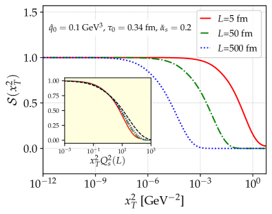
To make the interpretation of these results in terms of TWโ€™s more transparent we inserted Eq.โ€‰(10) in $\mathcal{S}(\boldsymbol{x}_{\perp})$ and plotted the result in Fig.โ€‰1 for several values of $L$. We see that the traveling wave propagates from right to left (from large to small $x_{T}$) with increasing $L$. However, once plotted in terms of xT2โ€‹Qs2superscriptsubscript๐‘ฅ๐‘‡2superscriptsubscript๐‘„๐‘ 2x_{T}^{2}Q_{s}^{2} as shown in the inset of Fig.โ€‰1, they all lie approximately on the same universal scaling function given by Eq.โ€‰(1)-(10) (dotted black curve). The observed deviations will be discussed in what follows.

Refer to caption

Figure 1: Dipole scattering amplitude as a function of the transverse dipole size squared $x_{T}^{2}$ for several values of the medium size. The inset shows the same curves as a function of the scaling variable xT2โ€‹Qs2โ€‹(L)superscriptsubscript๐‘ฅ๐‘‡2superscriptsubscript๐‘„๐‘ 2๐ฟx_{T}^{2}Q_{s}^{2}(L) compared to the scaling solution (dashed black) (color online).

Sub-asymptotic corrections.

We turn now to the calculation of the sub-asymptotic corrections to the geometric scaling solution (10). Near the wave front, typically for $x\gg 1$, we can look for a solution of the form

$\displaystyle\hat{q}(Y,\rho)$ =q^0โ€‹eฯsโ€‹(Y)โˆ’Yโ€‹eฮฒโ€‹xโ€‹Yฮฑโ€‹Gโ€‹(xYฮฑ),absentsubscript^๐‘ž0superscriptesubscript๐œŒ๐‘ ๐‘Œ๐‘Œsuperscripte๐›ฝ๐‘ฅsuperscript๐‘Œ๐›ผ๐บ๐‘ฅsuperscript๐‘Œ๐›ผ\displaystyle=\hat{q}_{0}{\rm e}^{\rho_{s}(Y)-Y}{\rm e}^{\beta x}Y^{\alpha}G\left(\frac{x}{Y^{\alpha}}\right)\,, (11)
ฯsโ€‹(Y)subscript๐œŒ๐‘ ๐‘Œ\displaystyle\rho_{s}(Y) $\displaystyle=cY+b\ln(Y)\,,$ (12)

inspired by the traveling waves ansatz that solves the BK equation Munierย andย Peschanski (2004) and more generally FKPP-like equations Fisher ; Kolmogorov (1937). Plugging this ansatz inside Eq.โ€‰(7), one gets a differential equation for $G(z)$. Because the coefficient of $Y$ and $Y^{\alpha}$ (assuming $\alpha>0$) in this equation must vanish, we recover the two previous constraints that fix the value of $c$ and $\beta$. Then, neglecting the power suppressed terms $Y^{-1}$ and $Y^{-\alpha-1}$, one finds

$\displaystyle-cY^{-\alpha}\frac{\textrm{d}^{2}}{\textrm{d}z^{2}}G(z)-\beta\alpha zY^{\alpha-1}\frac{\textrm{d}}{\textrm{d}z}G(z)$
$\displaystyle+\beta(-b\beta+b+\alpha)Y^{\alpha-1}G(z)=0\,.$ (13)

The homogeneity condition implies that the coefficient $\alpha$ must be equal to $1/2$ so that the deviation from the scaling form near the wave-front grows in a diffusive way as $Y$ increases.

For initial conditions such that $\beta<\beta$, the large $z$ behavior of the function $G(z)$ constrains the acceptable values of the coefficient in front of $G(z)$ in this differential equation. In fact, as shown in Brunetย andย Derrida (1997); Munierย andย Peschanski (2004), one must have $b\beta-b-\frac{1}{2}=1$, fixing $b$ to

$\displaystyle b$ $\displaystyle=-\frac{3}{2(1-\beta)}\,.$ (14)

This yields the solution

$$G\left(z=x/\sqrt{Y}\right)=\beta z\exp\left(-\frac{\beta z^{2}}{4c}\right)\,.$$ (15)

The value of $b$ we extract from this analysis is novel and a consequence of the non-linearity of the saturation boundary. In the linearized problem with the lower bound in the integral of Eq.โ€‰(7) set to $Y$ instead of ฯsโ€‹(Y)subscript๐œŒ๐‘ ๐‘Œ\rho_{s}(Y), one gets $b=-3/2$ from the analytic solution (5) Iancuย andย Triantafyllopoulos (2014), whereas in the non-linear case, we have bโ‰ƒโˆ’3/2โ€‹(1+ฮฑยฏs)similar-to-or-equals๐‘321subscriptยฏ๐›ผ๐‘ b\simeq-3/2(1+\sqrt{\bar{\alpha}_{s}}). The sub-leading term provides a correction to the saturation line which is parametrically of order ฮฑยฏsโ€‹lnโกYsubscriptยฏ๐›ผ๐‘ ๐‘Œ\sqrt{\bar{\alpha}_{s}}\ln Y and therefore dominant w.r.tโ€‰ single logarithmic corrections of order ฮฑยฏsโ€‹Yโˆผฮฑยฏssimilar-tosubscriptยฏ๐›ผ๐‘ ๐‘Œsubscriptยฏ๐›ผ๐‘ \bar{\alpha}_{s}Y\sim\sqrt{\bar{\alpha}_{s}} since in DLA Yโˆผ1/ฮฑยฏsโ‰ซ1similar-to๐‘Œ1subscriptยฏ๐›ผ๐‘ much-greater-than1Y\sim 1/\sqrt{\bar{\alpha}_{s}}\gg 1.

The TW solution (15) provides the functional form of $\hat{q}(Y,\rho)$ near the wave front, i.e.ย for x=ฯโˆ’ฯsโ€‹(Y)โˆผYโ‰ซ1๐‘ฅ๐œŒsubscript๐œŒ๐‘ ๐‘Œsimilar-to๐‘Œmuch-greater-than1x=\rho-\rho_{s}(Y)\sim\sqrt{Y}\gg 1 and fixes the value of the coefficient $b$ in the asymptotic expansion of ฯsโ€‹(Y)subscript๐œŒ๐‘ ๐‘Œ\rho_{s}(Y). For small values of $x$, one can find the scaling deviations by looking for a solution as a power series in $1/Y$ of the form q^โ€‹(Y,ฯ)=q^0โ€‹eฯsโ€‹(Y)โˆ’Yโ€‹fโ€‹(x)โ€‹โˆ‘nโ‰ฅ0Hnโ€‹(x)Yn^๐‘ž๐‘Œ๐œŒsubscript^๐‘ž0superscript๐‘’subscript๐œŒ๐‘ ๐‘Œ๐‘Œ๐‘“๐‘ฅsubscript๐‘›0subscript๐ป๐‘›๐‘ฅsuperscript๐‘Œ๐‘›\hat{q}(Y,\rho)=\hat{q}_{0}e^{\rho_{s}(Y)-Y}f(x)\sum_{n\geq 0}\frac{H_{n}(x)}{Y^{n}}. Plugging this form inside Eq.โ€‰(7) gives a second order differential equation for $H_{1}(x)$, whose initial conditions are constrained by the definition of Qssubscript๐‘„๐‘ Q_{s}. The solution to this equation reads: $H_{1}(x)=bx/[c^{2}(1+\beta x)][1+(c-1)(c+3)/(8c)x+(c-1)^{2}(1+c)/(48c^{2})x^{2}]$ 666See Supplemental Material 2 for detailed calculations.. The last term in this expression is included in the solution (15), as can be checked by expanding the function $G$ for large $Y$, but not the first two since Eq.โ€‰(15) is only valid at large $x$. Combining the scaling limit with its deviation provided by the function $G$ for $x\sim\sqrt{Y}$ and $H_{1}(x)$ for all $x$ up to powers of $1/Y^{2}$, our final result reads

q^โ€‹(Y,ฯ)=q^0โ€‹eฯsโ€‹(Y)โˆ’Yโ€‹expโก(ฮฒโ€‹xโˆ’ฮฒโ€‹x24โ€‹cโ€‹Y)^๐‘ž๐‘Œ๐œŒsubscript^๐‘ž0superscriptesubscript๐œŒ๐‘ ๐‘Œ๐‘Œ๐›ฝ๐‘ฅ๐›ฝsuperscript๐‘ฅ24๐‘๐‘Œ\displaystyle\hat{q}(Y,\rho)=\hat{q}_{0}\,{\rm e}^{\rho_{s}(Y)-Y}\exp\left(\beta x-\frac{\beta x^{2}}{4cY}\right)
$\displaystyle\times\left[1+\beta x+\frac{bx}{c^{2}Y}\left(1+\frac{\beta(c+4)x}{6}\right)+\mathcal{O}\left(\frac{1}{Y^{2}}\right)\right]\,,$ (16)

with ฯsโ€‹(Y)=cโ€‹Y+bโ€‹lnโก(Y)+constsubscript๐œŒ๐‘ ๐‘Œ๐‘๐‘Œ๐‘๐‘Œconst\rho_{s}(Y)=cY+b\ln(Y)+\rm const.

This solution is independent of the initial condition (for physically relevant ones), and only depends on the value of ฮฑยฏssubscriptยฏ๐›ผ๐‘ \bar{\alpha}_{s} via the coefficients $c$, $\beta$ and $b$. The resummed TMB distribution displays a universal behavior independent of the non-perturbative modeling of the tree-level distribution often used as an initial condition for non-linear small $x$ evolution McLerranย andย Venugopalan (1994a, b). It can therefore provide a model-independent functional form for the initial condition of the BK equation, that includes gluon fluctuations enhanced by double logs, ฮฑยฏsโ€‹ln2โกA1/3subscriptยฏ๐›ผ๐‘ superscript2superscript๐ด13\bar{\alpha}_{s}\ln^{2}A^{1/3}, inside the nucleus target to all orders.

Refer to caption

Figure 2: TMB distribution of a high energy gluon propagating though a dense medium of size $L$ at tree-level (dash-dotted line) and after resummation of the leading radiative corrections (solid red).The dotted black line is the scaling limit when $L\to\infty$ and the blue curve is our analytic result given by Eq.โ€‰(16) including sub-asymptotic corrections (color online).

III Super-diffusion and modification of Rutherford scattering

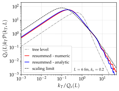
In this last section, we investigate the physical consequences of the scaling solution (10) for $\hat{q}(\boldsymbol{k}_{\perp}^{2})$ on the TMB distribution given by Eq.โ€‰(1), in particular at large $k_{T}$, where the distribution is characterized by rare events that are sensitive to the point-like nature of the medium scattering centers Dโ€™Eramoย etย al. (2013). First, it is straightforward to see that in the large $L$ limit, the TMB distribution $\mathcal{P}(k_{T})$ is only a function of kT/Qsโ€‹(L)subscript๐‘˜๐‘‡subscript๐‘„๐‘ ๐ฟk_{T}/Q_{s}(L). In Fig.โ€‰2, we show the distribution as a function of kT/Qsโ€‹(L)subscript๐‘˜๐‘‡subscript๐‘„๐‘ ๐ฟk_{T}/Q_{s}(L) with $Y=\ln(L/\tau_{0})=4$, for the following set-ups: (i) in dash-dotted grey, at tree-level, using Eq.โ€‰(2), (ii) after quantum evolution obtain by numerically solving Eqs.โ€‰(4) in red, (iii) in blue, using the expression Eq.โ€‰(16) that includes sub-asymptotic corrections to the scaling limit, (iv) finally, in dashed black, the scaling limit $Y\to\infty$ of Eq.โ€‰(16). Interestingly, the sub-asymptotic corrections account for the relatively large deviations between the asymptotic curve and the exact numerical result at the moderate value of $L=6$ fm.

The $k_{T}$ distribution exhibits two different regimes: the region of the peak, near Qsโ€‹(L)subscript๐‘„๐‘ ๐ฟQ_{s}(L) and the large $k_{T}$ tail, with kTโ‰ซQsโ€‹(L)much-greater-thansubscript๐‘˜๐‘‡subscript๐‘„๐‘ ๐ฟk_{T}\gg Q_{s}(L). These results can be interpreted in term of a special kind of random walk (here in momentum space) called Lรฉvy flight. Such a remarkable connection with statistical physics enables us to highlight some interesting features (i) self-similar dynamics (ii) super diffusion (iii) power-law tail with slower decay than the Rutherford $\boldsymbol{k}_{\perp}^{-4}$ behavior.

In order to further the connection with the physics of anomalous diffusion, consider the scaling limit of the TMB distribution in the vicinity of the peak where the shape of the distribution is controlled by the first line in Eq.โ€‰(10). Using this solution, one finds that ๐’ฎโ€‹(๐’™โŸ‚)โ‰ƒexpโก[โˆ’14โ€‹CRNcโ€‹(|๐’™โŸ‚|โ€‹Qs)2โˆ’4โ€‹ฮฒ]similar-to-or-equals๐’ฎsubscript๐’™perpendicular-to14subscript๐ถ๐‘…subscript๐‘๐‘superscriptsubscript๐’™perpendicular-tosubscript๐‘„๐‘ 24๐›ฝ\mathcal{S}(\boldsymbol{x}_{\perp})\simeq\exp\left[-\,\frac{1}{4}\frac{C_{R}}{N_{c}}\,(|\boldsymbol{x}_{\perp}|Q_{s})^{2-4\beta}\right]. In momentum space, it implies that the distribution $\mathcal{P}(\boldsymbol{k}_{\perp},L)$ satisfies a generalized Fokker-Planck equation, $\partial\mathcal{P}/\partial L\propto\ -(-\Delta)^{1-2\beta}\mathcal{P}$, where the so-called fractional Laplace operator $(-\Delta)^{\gamma/2}$ is defined by its Fourier transform $|\boldsymbol{x}_{\perp}|^{\gamma}$ Hilfer ; Kwaล›nicki (2017). This fractional diffusion equation (without external potential) is satisfied by the probability density for the position of a particle undergoing a Lรฉvy flight process in two dimension Dubkovย etย al. (2008) with stability index ฮณ=2โˆ’4โ€‹ฮฒโ‰ƒ2โˆ’4โ€‹ฮฑs+๐’ชโ€‹(ฮฑs)๐›พ24๐›ฝsimilar-to-or-equals24subscript๐›ผ๐‘ ๐’ชsubscript๐›ผ๐‘ \gamma=2-4\beta\simeq 2-4\sqrt{\alpha_{s}}+\mathcal{O}(\alpha_{s}).

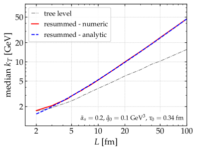
Because of its heavy tail (to be discussed thereafter), the mean $k_{T}^{2}$ of the TMB distribution is not defined. Nevertheless, it is possible to introduce a measure of the characteristic width of the $k_{T}$ distribution, and study its behavior as a function of the medium size $L$. In what follows, we shall use the median value $\langle k_{T}\rangle_{\rm med}$ of $k_{T}\mathcal{P}(k_{T})$ 777 Another possibility is to define fractional moments Metzlerย andย Nonnenmacher (2002); Dubkovย etย al. (2008) which is shown in Fig.ย 3 for three different scenarios. In grey, we plot the tree-level resulting from Eq.ย (1) and (2). The median scales approximately like $(L\ln L)^{1/2}$, which up to the logarithmic factor resulting from the Coulomb logarithm in Eq.ย (2), exhibits the standard diffusion scaling. The red line is the median of the $k_{T}$ distribution obtained using the resummed value of $\hat{q}$ with fixed coupling, after numerical resolution of Eqs.โ€‰(4). We then compare this result with our analytic prediction (12) (assuming โŸจkTโŸฉmedโˆQsproportional-tosubscriptdelimited-โŸจโŸฉsubscript๐‘˜๐‘‡medsubscript๐‘„๐‘ \langle k_{T}\rangle_{\rm med}\propto Q_{s} 888the unknown pre-factor is determined by a fit to the numerical result at large $L$), $\langle k_{T}\rangle_{\rm med}\propto L^{{}^{\frac{c}{2}+\frac{b}{2}\frac{\ln(Y)}{Y}}}$, which is represented in blue in Fig.โ€‰3 . Remarkably, the agreement is excellent down to rather small values of $L\sim 3$ fm. Since $c/2>1/2$, the median grows faster than $\sqrt{L}$ at large $L$, illustrating the super-diffusive behavior of TMB beyond leading order, with a deviation to the standard diffusion of order ฮฑยฏssubscriptยฏ๐›ผ๐‘ \sqrt{\bar{\alpha}_{s}}.

Refer to caption

Figure 3: System size dependence of the median of the TMB distribution at tree-level (grey line) and after numerical resummation of radiative corrections (red line). The dashed blue line is our analytic prediction given by Eq.โ€‰(12).

Heavy-tailed distribution.

Another important aspect of Lรฉvy flights is the power law decay of the step length distribution for a Lรฉvy walker Klafterย etย al. (1987); Metzlerย etย al. (1999). This reflects the fact that long jumps with arbitrary length may occur with non-negligible probability. In the problem at hand, this power-law tail can also be understood as a consequence of the self-similar nature of overlapping successive gluon fluctuations.

The tail of the TMB distribution is controlled by the large $\boldsymbol{k}_{\perp}^{2}$ behavior of $\hat{q}(\boldsymbol{k}_{\perp}^{2})$, and consequently, by the exponential in the second line in (10). Note, however, that the scaling limit encompasses two stability indices: one controlling the peak and the median, as discussed above, while the other controls the tail of the distribution (cf. (10)). Without loss of generality, one can derive the leading behavior of $\mathcal{P}(\boldsymbol{k}_{\perp})$ at large $\boldsymbol{k}_{\perp}$ by expanding the dipole S-matrix for small dipole sizes, as a result the Fourier transform can be approximated by 999See Supplemental Material 3 for detailed calculations.:

$\displaystyle\mathcal{P}(\boldsymbol{k}_{\perp})\sim\vec{\nabla}_{\boldsymbol{k}_{\perp}}^{2}\frac{\pi}{\boldsymbol{k}_{\perp}^{2}}\frac{{\rm d}\hat{q}(\boldsymbol{k}_{\perp}^{2})L}{{\rm d}\ln\boldsymbol{k}_{\perp}^{2}}\,,$ (17)

up to logarithmically suppressed terms. This formula quantifies the deviations from the Rutherford scattering cross-section that are induced by radiative corrections. Applying Eq.ย (17) to our scaling solution (10), one finds the tail

๐’ซโ€‹(๐’ŒโŸ‚)โˆ1Qs2โ€‹(L)โ€‹(Qs2โ€‹(L)๐’ŒโŸ‚2)ฮฝ,proportional-to๐’ซsubscript๐’Œperpendicular-to1superscriptsubscript๐‘„๐‘ 2๐ฟsuperscriptsuperscriptsubscript๐‘„๐‘ 2๐ฟsuperscriptsubscript๐’Œperpendicular-to2๐œˆ\mathcal{P}(\boldsymbol{k}_{\perp})\propto\frac{1}{Q_{s}^{2}(L)}\left(\frac{Q_{s}^{2}(L)}{\boldsymbol{k}_{\perp}^{2}}\right)^{\nu}\,, (18)

with $\nu=2-\beta+\mathcal{O}(\ln(x)/x)$ and x=lnโก(๐’ŒโŸ‚2/Qs2โ€‹(L))๐‘ฅsuperscriptsubscript๐’Œperpendicular-to2superscriptsubscript๐‘„๐‘ 2๐ฟx=\ln(\boldsymbol{k}_{\perp}^{2}/Q_{s}^{2}(L)). The corrections to the power-law behavior are due to the pre-factor in the second line of (10). The power of the tail deviates from the tree level Rutherford behavior by โˆผโˆ’2โ€‹ฮฑยฏssimilar-toabsent2subscriptยฏ๐›ผ๐‘ \sim-2\sqrt{\bar{\alpha}_{s}}. The form of $\nu$ is correct in the strict scaling limit $L\to\infty$. For finite $L$ values, the $1/\boldsymbol{k}_{\perp}^{4}$ tail is recovered at very large $k_{T}$, as can be inferred from Eq.โ€‰(5) which yields ฮฝ=2โˆ’2โ€‹ฮฑยฏsโ€‹Y/x๐œˆ22subscriptยฏ๐›ผ๐‘ ๐‘Œ๐‘ฅ\nu=2-2\sqrt{\bar{\alpha}_{s}Y/x} (when $x\gg Y$). The fact that geometric scaling extends in the tail region is known in the context of saturation physics as the โ€œextended geometric scaling windowโ€ corresponding to Qsโ‰ชkTโ‰ชQs2/ฮผmuch-less-thansubscript๐‘„๐‘ subscript๐‘˜๐‘‡much-less-thansuperscriptsubscript๐‘„๐‘ 2๐œ‡Q_{s}\ll k_{T}\ll Q_{s}^{2}/\mu.

Finally, note that this analysis is valid so long as $E/k_{T}^{2}\gg L$, where $E$ is the energy of the fast parton. This allows us to neglect the quantum diffusion of the dipole in the medium. In the opposite case the quantum phase is suppressed when $E/k_{T}^{2}\ll\tau\ll L$ and the evolution is expected to be of DGLAP type with the substitution $\ln L/\tau_{0}\to\ln E/(k_{T}^{2}\tau_{0})$ 101010This regime was discussed in Casalderrey-Solanaย andย Wang (2008)..

Conclusion.

In summary, we have studied the transverse momentum distribution of a high-energy parton propagating through a dense QCD medium, including resummation of radiative corrections within a modified double logarithmic approximation which accounts for the non-linear dynamics due to multiple scatterings that restrict the phase space for quantum fluctuations. We have found that the non-linearity and self-similarity of overlapping multiple gluon radiations lead to a universal scaling limit at large system sizes, which exhibits a super-diffusive regime and a power-law decay akin to Lรฉvy flights. Although at very high $\boldsymbol{k}_{\perp}$, the distribution is characterized by point-like interactions of Rutherford type, for moderately large $\boldsymbol{k}_{\perp}$ we observe a weaker power due to the non-local nature of the interactions which is the hallmark of scale invariant phenomena.

Concerning phenomenological applications, we point out the relevance of our analytic solutions in the study of nuclear structure at high energy as it provides a new initial condition for non-linear evolution of the gluon distribution. We leave for future work the question of the experimental detection of this emergent QCD phenomenon in heavy ion collisions as well as running coupling corrections which are expected to yield mild scaling violations.

Acknowledgements This work was supported by the U.S. Department of Energy, Office of Science, Office of Nuclear Physics, under contract No. DE- SC0012704. Y. M.-T. acknowledges support from the RHIC Physics Fellow Program of the RIKEN BNL Research Center.

References

Appendix A 1. Numerical implementation of the evolution equation

Differential problem.

We discuss here the numerical method used to solve the evolution equation for $\hat{q}$ with exact treatment of the saturation boundary for the gluon emission phase space. The evolution equation in differential form reads

$\displaystyle\frac{\partial\hat{q}(\tau,\boldsymbol{k}_{\perp}^{2})}{\partial\ln(\tau)}$ =ฮฑยฏsโ€‹โˆซQs2โ€‹(ฯ„)๐’ŒโŸ‚2dโ€‹๐’ŒโŸ‚โ€ฒโฃ2๐’ŒโŸ‚โ€ฒโฃ2โ€‹q^โ€‹(ฯ„,๐’ŒโŸ‚โ€ฒโฃ2)absentsubscriptยฏ๐›ผ๐‘ superscriptsubscriptsubscriptsuperscript๐‘„2๐‘ ๐œsuperscriptsubscript๐’Œperpendicular-to2dsuperscriptsubscript๐’Œperpendicular-toโ€ฒ2superscriptsubscript๐’Œperpendicular-toโ€ฒ2^๐‘ž๐œsuperscriptsubscript๐’Œperpendicular-toโ€ฒ2\displaystyle=\bar{\alpha}_{s}\int_{Q^{2}_{s}(\tau)}^{\boldsymbol{k}_{\perp}^{2}}\frac{{\rm d}\boldsymbol{k}_{\perp}^{\prime 2}}{\boldsymbol{k}_{\perp}^{\prime 2}}\hat{q}(\tau,\boldsymbol{k}_{\perp}^{\prime 2}) (19)
Qs2โ€‹(ฯ„)subscriptsuperscript๐‘„2๐‘ ๐œ\displaystyle Q^{2}_{s}(\tau) =q^โ€‹(ฯ„,Qs2โ€‹(ฯ„))โ€‹ฯ„.absent^๐‘ž๐œsuperscriptsubscript๐‘„๐‘ 2๐œ๐œ\displaystyle=\hat{q}(\tau,Q_{s}^{2}(\tau))\tau\,. (20)

The existence of a solution is not guaranteed since the boundary of the $\boldsymbol{k}_{\perp}^{\prime}$ integral depends on $\hat{q}(\tau,\boldsymbol{k}_{\perp}^{2})$ itself. That said, it is possible to show that the two equations above constitute a well defined initial-value problem. To do so, we differentiate the l.h.s. of Eq.ย (20) w.r.t. $\tau$:

dโ€‹Qs2โ€‹(ฯ„)dโ€‹ฯ„dsuperscriptsubscript๐‘„๐‘ 2๐œd๐œ\displaystyle\frac{{\rm d}Q_{s}^{2}(\tau)}{{\rm d}\tau} =dโ€‹q^โ€‹(ฯ„,Qs2โ€‹(ฯ„))dโ€‹ฯ„โ€‹ฯ„+q^โ€‹(ฯ„,Qs2โ€‹(ฯ„)),absentd^๐‘ž๐œsuperscriptsubscript๐‘„๐‘ 2๐œd๐œ๐œ^๐‘ž๐œsuperscriptsubscript๐‘„๐‘ 2๐œ\displaystyle=\frac{{\rm d}\hat{q}(\tau,Q_{s}^{2}(\tau))}{{\rm d}\tau}\tau+\hat{q}(\tau,Q_{s}^{2}(\tau))\,, (21)
=โˆ‚q^โ€‹(ฯ„,๐’ŒโŸ‚2)โˆ‚๐’ŒโŸ‚2|๐’ŒโŸ‚2=Qs2โ€‹(ฯ„)โ€‹dโ€‹Qs2โ€‹(ฯ„)dโ€‹ฯ„โ€‹ฯ„+1ฯ„โ€‹Qs2โ€‹(ฯ„).absentevaluated-at^๐‘ž๐œsuperscriptsubscript๐’Œperpendicular-to2superscriptsubscript๐’Œperpendicular-to2superscriptsubscript๐’Œperpendicular-to2subscriptsuperscript๐‘„2๐‘ ๐œdsubscriptsuperscript๐‘„2๐‘ ๐œd๐œ๐œ1๐œsuperscriptsubscript๐‘„๐‘ 2๐œ\displaystyle=\frac{\partial\hat{q}(\tau,\boldsymbol{k}_{\perp}^{2})}{\partial\boldsymbol{k}_{\perp}^{2}}\Bigg{|}_{\boldsymbol{k}_{\perp}^{2}=Q^{2}_{s}(\tau)}\frac{{\rm d}Q^{2}_{s}(\tau)}{{\rm d}\tau}\tau+\frac{1}{\tau}Q_{s}^{2}(\tau)\,. (22)

The partial derivative of $\hat{q}(\tau,\boldsymbol{k}_{\perp}^{2})$ can be obtained from the evolution equation in its integral form:

$\displaystyle\hat{q}(\tau,\boldsymbol{k}_{\perp}^{2})$ =q^โ€‹(ฯ„0,๐’ŒโŸ‚2)+ฮฑยฏsโ€‹โˆซฯ„0ฯ„dโ€‹ฯ„โ€ฒฯ„โ€ฒโ€‹โˆซQs2โ€‹(ฯ„โ€ฒ)๐’ŒโŸ‚2dโ€‹๐’ŒโŸ‚โ€ฒโฃ2๐’ŒโŸ‚โ€ฒโฃ2โ€‹q^โ€‹(ฯ„โ€ฒ,๐’ŒโŸ‚โ€ฒโฃ2),absent^๐‘žsubscript๐œ0superscriptsubscript๐’Œperpendicular-to2subscriptยฏ๐›ผ๐‘ superscriptsubscriptsubscript๐œ0๐œdsuperscript๐œโ€ฒsuperscript๐œโ€ฒsuperscriptsubscriptsubscriptsuperscript๐‘„2๐‘ superscript๐œโ€ฒsuperscriptsubscript๐’Œperpendicular-to2dsuperscriptsubscript๐’Œperpendicular-toโ€ฒ2superscriptsubscript๐’Œperpendicular-toโ€ฒ2^๐‘žsuperscript๐œโ€ฒsuperscriptsubscript๐’Œperpendicular-toโ€ฒ2\displaystyle=\hat{q}(\tau_{0},\boldsymbol{k}_{\perp}^{2})+\bar{\alpha}_{s}\int_{\tau_{0}}^{\tau}\frac{{\rm d}\tau^{\prime}}{\tau^{\prime}}\int_{Q^{2}_{s}(\tau^{\prime})}^{\boldsymbol{k}_{\perp}^{2}}\frac{{\rm d}\boldsymbol{k}_{\perp}^{\prime 2}}{\boldsymbol{k}_{\perp}^{\prime 2}}\hat{q}(\tau^{\prime},\boldsymbol{k}_{\perp}^{\prime 2})\,, (23)
=q^โ€‹(ฯ„0,๐’ŒโŸ‚2)+ฮฑยฏsโ€‹โˆซQs2โ€‹(ฯ„0)๐’ŒโŸ‚2dโ€‹๐’ŒโŸ‚โ€ฒโฃ2๐’ŒโŸ‚โ€ฒโฃ2โ€‹โˆซฯ„0minโ€‹(ฯ„,ฯ„sโ€‹(๐’ŒโŸ‚โ€ฒโฃ2))dโ€‹ฯ„โ€ฒฯ„โ€ฒโ€‹q^โ€‹(ฯ„โ€ฒ,๐’ŒโŸ‚โ€ฒโฃ2),absent^๐‘žsubscript๐œ0superscriptsubscript๐’Œperpendicular-to2subscriptยฏ๐›ผ๐‘ superscriptsubscriptsubscriptsuperscript๐‘„2๐‘ subscript๐œ0superscriptsubscript๐’Œperpendicular-to2dsuperscriptsubscript๐’Œperpendicular-toโ€ฒ2superscriptsubscript๐’Œperpendicular-toโ€ฒ2superscriptsubscriptsubscript๐œ0min๐œsubscript๐œ๐‘ superscriptsubscript๐’Œperpendicular-toโ€ฒ2dsuperscript๐œโ€ฒsuperscript๐œโ€ฒ^๐‘žsuperscript๐œโ€ฒsuperscriptsubscript๐’Œperpendicular-toโ€ฒ2\displaystyle=\hat{q}(\tau_{0},\boldsymbol{k}_{\perp}^{2})+\bar{\alpha}_{s}\int_{Q^{2}_{s}(\tau_{0})}^{\boldsymbol{k}_{\perp}^{2}}\frac{{\rm d}\boldsymbol{k}_{\perp}^{\prime 2}}{\boldsymbol{k}_{\perp}^{\prime 2}}\int_{\tau_{0}}^{\mathrm{min}(\tau,\tau_{s}(\boldsymbol{k}_{\perp}^{\prime 2}))}\frac{{\rm d}\tau^{\prime}}{\tau^{\prime}}\hat{q}(\tau^{\prime},\boldsymbol{k}_{\perp}^{\prime 2})\,, (24)

with ฯ„sโ€‹(๐’ŒโŸ‚2)subscript๐œ๐‘ superscriptsubscript๐’Œperpendicular-to2\tau_{s}(\boldsymbol{k}_{\perp}^{2}) the inverse function of Qs2โ€‹(ฯ„)subscriptsuperscript๐‘„2๐‘ ๐œQ^{2}_{s}(\tau) that satisfies then ฯ„sโ€‹(Qs2โ€‹(ฯ„))=ฯ„subscript๐œ๐‘ subscriptsuperscript๐‘„2๐‘ ๐œ๐œ\tau_{s}(Q^{2}_{s}(\tau))=\tau. One can then compute the derivative w.r.t. $\boldsymbol{k}_{\perp}^{2}$, evaluated at Qs2โ€‹(ฯ„)superscriptsubscript๐‘„๐‘ 2๐œQ_{s}^{2}(\tau):

โˆ‚q^โ€‹(ฯ„,๐’ŒโŸ‚2)โˆ‚๐’ŒโŸ‚2|๐’ŒโŸ‚2=Qs2โ€‹(ฯ„)=โˆ‚q^โ€‹(ฯ„0,๐’ŒโŸ‚2)โˆ‚๐’ŒโŸ‚2|๐’ŒโŸ‚2=Qs2โ€‹(ฯ„)+ฮฑยฏsQs2โ€‹(ฯ„)โ€‹โˆซฯ„0ฯ„dโ€‹ฯ„โ€ฒฯ„โ€ฒโ€‹q^โ€‹(ฯ„โ€ฒ,Qs2โ€‹(ฯ„)).evaluated-at^๐‘ž๐œsuperscriptsubscript๐’Œperpendicular-to2superscriptsubscript๐’Œperpendicular-to2superscriptsubscript๐’Œperpendicular-to2subscriptsuperscript๐‘„2๐‘ ๐œevaluated-at^๐‘žsubscript๐œ0superscriptsubscript๐’Œperpendicular-to2superscriptsubscript๐’Œperpendicular-to2superscriptsubscript๐’Œperpendicular-to2subscriptsuperscript๐‘„2๐‘ ๐œsubscriptยฏ๐›ผ๐‘ subscriptsuperscript๐‘„2๐‘ ๐œsuperscriptsubscriptsubscript๐œ0๐œdsuperscript๐œโ€ฒsuperscript๐œโ€ฒ^๐‘žsuperscript๐œโ€ฒsubscriptsuperscript๐‘„2๐‘ ๐œ\displaystyle\frac{\partial\hat{q}(\tau,\boldsymbol{k}_{\perp}^{2})}{\partial\boldsymbol{k}_{\perp}^{2}}\Bigg{|}_{\boldsymbol{k}_{\perp}^{2}=Q^{2}_{s}(\tau)}=\frac{\partial\hat{q}(\tau_{0},\boldsymbol{k}_{\perp}^{2})}{\partial\boldsymbol{k}_{\perp}^{2}}\Bigg{|}_{\boldsymbol{k}_{\perp}^{2}=Q^{2}_{s}(\tau)}+\frac{\bar{\alpha}_{s}}{Q^{2}_{s}(\tau)}\int_{\tau_{0}}^{\tau}\frac{{\rm d}\tau^{\prime}}{\tau^{\prime}}\hat{q}(\tau^{\prime},Q^{2}_{s}(\tau))\,. (25)

Finally, we end up with the following differential equation for Qs2โ€‹(ฯ„)subscriptsuperscript๐‘„2๐‘ ๐œQ^{2}_{s}(\tau):

(1โˆ’ฯ„โ€‹โˆ‚q^โ€‹(ฯ„0,๐’ŒโŸ‚2)โˆ‚๐’ŒโŸ‚2|๐’ŒโŸ‚2=Qs2โ€‹(ฯ„)โˆ’ฮฑยฏsโ€‹ฯ„Qs2โ€‹(ฯ„)โ€‹โˆซฯ„0ฯ„dโ€‹ฯ„โ€ฒฯ„โ€ฒโ€‹q^โ€‹(ฯ„โ€ฒ,Qs2โ€‹(ฯ„)))โ€‹dโ€‹Qs2dโ€‹lnโก(ฯ„)=Qs2โ€‹(ฯ„).1evaluated-at๐œ^๐‘žsubscript๐œ0superscriptsubscript๐’Œperpendicular-to2superscriptsubscript๐’Œperpendicular-to2superscriptsubscript๐’Œperpendicular-to2subscriptsuperscript๐‘„2๐‘ ๐œsubscriptยฏ๐›ผ๐‘ ๐œsubscriptsuperscript๐‘„2๐‘ ๐œsuperscriptsubscriptsubscript๐œ0๐œdsuperscript๐œโ€ฒsuperscript๐œโ€ฒ^๐‘žsuperscript๐œโ€ฒsubscriptsuperscript๐‘„2๐‘ ๐œdsuperscriptsubscript๐‘„๐‘ 2d๐œsubscriptsuperscript๐‘„2๐‘ ๐œ\left(1-\tau\frac{\partial\hat{q}(\tau_{0},\boldsymbol{k}_{\perp}^{2})}{\partial\boldsymbol{k}_{\perp}^{2}}\Bigg{|}_{\boldsymbol{k}_{\perp}^{2}=Q^{2}_{s}(\tau)}-\frac{\bar{\alpha}_{s}\tau}{Q^{2}_{s}(\tau)}\int_{\tau_{0}}^{\tau}\frac{{\rm d}\tau^{\prime}}{\tau^{\prime}}\hat{q}(\tau^{\prime},Q^{2}_{s}(\tau))\right)\frac{{\rm d}Q_{s}^{2}}{{\rm d}\ln(\tau)}=Q^{2}_{s}(\tau)\,. (26)

This equation is more convenient from a numerical point of view because one does not need to solve the implicit equation defining Qs2โ€‹(ฯ„)subscriptsuperscript๐‘„2๐‘ ๐œQ^{2}_{s}(\tau) at each small step in $\tau$. Instead, one solves two coupled integro-differential equations of order 1.

The initial condition $\hat{q}(\tau_{0},\boldsymbol{k}_{\perp}^{2})$ enables to define a bare saturation boundary. For example, we may assume that $\hat{q}(\tau_{0},\boldsymbol{k}_{\perp}^{2})=\hat{q}_{0}f_{0}(\boldsymbol{k}_{\perp}^{2})$ with some function $f_{0}(\boldsymbol{k}_{\perp}^{2})$. Defining $Y=\ln(\tau/\tau_{0})$ and $\rho=\ln\left(\frac{\boldsymbol{k}_{\perp}^{2}}{\hat{q}_{0}\tau_{0}}\right)$, and the following dimensionless quantities

q^dโ€‹(Y,ฯ)=q^โ€‹(ฯ„0โ€‹eY,q^0โ€‹ฯ„0โ€‹eฯ)q^0,ฯsโ€‹(Y)=lnโก(Qs2โ€‹(ฯ„0โ€‹eY)q^0โ€‹ฯ„0),formulae-sequencesubscript^๐‘ž๐‘‘๐‘Œ๐œŒ^๐‘žsubscript๐œ0superscripte๐‘Œsubscript^๐‘ž0subscript๐œ0superscripte๐œŒsubscript^๐‘ž0subscript๐œŒ๐‘ ๐‘Œsubscriptsuperscript๐‘„2๐‘ subscript๐œ0superscripte๐‘Œsubscript^๐‘ž0subscript๐œ0\displaystyle\hat{q}_{d}(Y,\rho)=\frac{\hat{q}\left(\tau_{0}{\rm e}^{Y},\hat{q}_{0}\tau_{0}{\rm e}^{\rho}\right)}{\hat{q}_{0}}\,,\qquad\rho_{s}(Y)=\ln\left(\frac{Q^{2}_{s}(\tau_{0}{\rm e}^{Y})}{\hat{q}_{0}\tau_{0}}\right)\,, (27)

the system of differential equation reads finally

$\displaystyle\frac{\partial\hat{q}_{d}(Y,\rho)}{\partial Y}$ $\displaystyle=\bar{\alpha}_{s}\int_{\rho_{s}(Y)}^{\rho}{\rm d}\rho^{\prime}\hat{q}_{d}(Y,\rho^{\prime}\,,)$ (28)
dโ€‹ฯsโ€‹(Y)dโ€‹Ydsubscript๐œŒ๐‘ ๐‘Œd๐‘Œ\displaystyle\frac{{\rm d}\rho_{s}(Y)}{{\rm d}Y} =1+eYโˆ’ฯsโ€‹(Y)โ€‹[dโ€‹f0dโ€‹ฯ|ฯ=ฯsโ€‹(Y)+ฮฑยฏsโ€‹โˆซ0YdYโ€ฒโ€‹q^dโ€‹(Yโ€ฒ,ฯsโ€‹(Y))]โ€‹dโ€‹ฯsโ€‹(Y)dโ€‹Y.absent1superscripte๐‘Œsubscript๐œŒ๐‘ ๐‘Œdelimited-[]evaluated-atdsubscript๐‘“0d๐œŒ๐œŒsubscript๐œŒ๐‘ ๐‘Œsubscriptยฏ๐›ผ๐‘ superscriptsubscript0๐‘Œdifferential-dsuperscript๐‘Œโ€ฒsubscript^๐‘ž๐‘‘superscript๐‘Œโ€ฒsubscript๐œŒ๐‘ ๐‘Œdsubscript๐œŒ๐‘ ๐‘Œd๐‘Œ\displaystyle=1+{\rm e}^{Y-\rho_{s}(Y)}\left[\left.\frac{{\rm d}f_{0}}{{\rm d}\rho}\right|_{\rho=\rho_{s}(Y)}+\bar{\alpha}_{s}\int_{0}^{Y}{\rm d}Y^{\prime}\hat{q}_{d}(Y^{\prime},\rho_{s}(Y))\right]\frac{{\rm d}\rho_{s}(Y)}{{\rm d}Y}\,. (29)

The second equation deserves some comments: (i) the first ($1$) term is to be associated with the linearized saturation line Qs2โ€‹(ฯ„)=q^0โ€‹ฯ„subscriptsuperscript๐‘„2๐‘ ๐œsubscript^๐‘ž0๐œQ^{2}_{s}(\tau)=\hat{q}_{0}\tau, since the solution of dโ€‹ฯsโ€‹(Y)dโ€‹Y=1๐‘‘subscript๐œŒ๐‘ ๐‘Œ๐‘‘๐‘Œ1\frac{d\rho_{s}(Y)}{dY}=1 with ฯsโ€‹(0)=0subscript๐œŒ๐‘ 00\rho_{s}(0)=0 is ฯsโ€‹(Y)=Ysubscript๐œŒ๐‘ ๐‘Œ๐‘Œ\rho_{s}(Y)=Y which gives Qs2โ€‹(ฯ„)=q^0โ€‹ฯ„subscriptsuperscript๐‘„2๐‘ ๐œsubscript^๐‘ž0๐œQ^{2}_{s}(\tau)=\hat{q}_{0}\tau, (ii) the term proportional to ฮฑssubscript๐›ผ๐‘ \alpha_{s} inside the square brackets is the back-reaction of the quantum evolution of $\hat{q}$ on the saturation boundary.

Euler method.

This evolution equation is solved using the Euler method, by discretizing the time $Y\in[0,Y_{L}=\ln(L/\tau_{0})]$. The transverse momentum space is also discretized $\rho\in[0,\rho_{\rm max}]$ and the $\rho$ integrals are evaluated using the trapezoidal rule. The initial condition $\hat{q}_{d}(0,\rho)=f_{0}(\rho)$ to the differential problem is given by the tree-level functional form of $\hat{q}_{d}(\rho)$, in which we keep the leading logarithmic dependence. In the hard thermal loop calculation of $\hat{q}$ at leading order, this logarithmic dependence reads $\hat{q}(\boldsymbol{k}_{\perp}^{2})=\hat{q}_{0}\ln(\boldsymbol{k}_{\perp}^{2}/\mu^{2})$ (cf.ย Eq.ย (2)) with $\hat{q}_{0}=\frac{g^{2}}{4\pi}C_{R}m_{D}^{2}T$ and $\mu^{2}=\frac{m_{D}^{2}}{4}{\rm e}^{-2+2\gamma_{E}}$. Using this expression as the initial condition $\hat{q}(\tau_{0},\boldsymbol{k}_{\perp}^{2})$ at the initial time $\tau_{0}$, the defining equation for Qs2โ€‹(ฯ„0)subscriptsuperscript๐‘„2๐‘ subscript๐œ0Q^{2}_{s}(\tau_{0}) reads Qs2โ€‹(ฯ„0)=q^โ€‹(Qs2)โ€‹ฯ„0superscriptsubscript๐‘„๐‘ 2subscript๐œ0^๐‘žsuperscriptsubscript๐‘„๐‘ 2subscript๐œ0Q_{s}^{2}(\tau_{0})=\hat{q}(Q_{s}^{2})\tau_{0} or equivalently expโก(ฯsโ€‹(0))=ฯsโ€‹(0)+lnโก(q^0โ€‹ฯ„0ฮผ2)subscript๐œŒ๐‘ 0subscript๐œŒ๐‘ 0subscript^๐‘ž0subscript๐œ0superscript๐œ‡2\exp\left(\rho_{s}(0)\right)=\rho_{s}(0)+\ln\left(\frac{\hat{q}_{0}\tau_{0}}{\mu^{2}}\right). This equation has a real solution if and only if

$$\ln\left(\frac{\hat{q}_{0}\tau_{0}}{\mu^{2}}\right)\geqslant 1\Longrightarrow\tau_{0}\geqslant\frac{{\rm e}\mu^{2}}{\hat{q}_{0}}=\frac{{\rm e}^{-1+2\gamma_{E}}\pi}{g^{2}T}\,.$$ (30)

Thus, we shall use $\tau_{0}={\rm e}^{-1+2\gamma_{E}}\pi/(g^{2}T)$ which is of the order of the mean free path $\sim 1/g^{2}T$. With this choice, ฯsโ€‹(0)=0subscript๐œŒ๐‘ 00\rho_{s}(0)=0 and

$$f_{0}(\rho)=\rho+1,\,\qquad\frac{{\rm d}f_{0}(\rho)}{{\rm d}\rho}=1\,.$$ (31)

From a numerical standpoint, the initial condition $f_{0}(\rho)=\rho+1$ requires some care because the naive Euler method fails at $Y=0$, since from Eq.ย (29), the derivative of ฯsโ€‹(Y)subscript๐œŒ๐‘ ๐‘Œ\rho_{s}(Y) w.r.t. $Y$ in $Y=0$ diverges. One needs then to initialize the Euler method in the middle of the first bin using

ฯsโ€‹(ฮ”โ€‹Y2)=ฮ”โ€‹Y2+lnโก[โˆ’Wโ€‹(โˆ’eโˆ’ฮ”โ€‹Y2โˆ’1,โˆ’1)],subscript๐œŒ๐‘ ฮ”๐‘Œ2ฮ”๐‘Œ2Wsuperscripteฮ”๐‘Œ211\rho_{s}\left(\frac{\Delta Y}{2}\right)=\frac{\Delta Y}{2}+\ln\left[-\mathrm{W}\left(-{\rm e}^{-\frac{\Delta Y}{2}-1},-1\right)\right]\,, (32)

where $\mathrm{W}(x,n)$ is the Lambert function on the $n^{\rm th}$ branch.

Appendix B 2. Sub-asymptotic corrections away from the wave front

In this section, we compute the sub-asymptotic corrections to the scaling solution, in the regime where $x$ is not necessarily large. We try the following ansatz:

$\displaystyle\hat{q}_{d}(Y,\rho)$ =eฯsโ€‹(Y)โˆ’Yโ€‹fโ€‹(x)โ€‹(1+bโ€‹H1โ€‹(x)Y+๐’ชโ€‹(1Y)),absentsuperscript๐‘’subscript๐œŒ๐‘ ๐‘Œ๐‘Œ๐‘“๐‘ฅ1๐‘subscript๐ป1๐‘ฅ๐‘Œ๐’ช1๐‘Œ\displaystyle=e^{\rho_{s}(Y)-Y}f(x)\left(1+\frac{bH_{1}(x)}{Y}+{\cal O}\left(\frac{1}{Y}\right)\right)\,, (33)
ฯsโ€‹(Y)subscript๐œŒ๐‘ ๐‘Œ\displaystyle\rho_{s}(Y) $\displaystyle=cY+b\ln(Y)+{\cal O}(\ln(Y))\,.$ (34)

The form is inspired by the large $Y$ expansion of the travelling wave ansatz. We have indeed, with $G$ given by Eq.โ€‰(15):

q^dโ€‹(Y,ฯ)โ‰ƒeฯsโ€‹(Y)โˆ’Yโ€‹ฮฒโ€‹xโ€‹eฮฒโ€‹xโ€‹(1โˆ’ฮฒโ€‹x24โ€‹cโ€‹Y+๐’ชโ€‹(1Y)),similar-to-or-equalssubscript^๐‘ž๐‘‘๐‘Œ๐œŒsuperscript๐‘’subscript๐œŒ๐‘ ๐‘Œ๐‘Œ๐›ฝ๐‘ฅsuperscript๐‘’๐›ฝ๐‘ฅ1๐›ฝsuperscript๐‘ฅ24๐‘๐‘Œ๐’ช1๐‘Œ\hat{q}_{d}(Y,\rho)\simeq e^{\rho_{s}(Y)-Y}\beta xe^{\beta x}\left(1-\frac{\beta x^{2}}{4cY}+{\cal O}\left(\frac{1}{Y}\right)\right)\,, (35)

for $x\gg 1$ and large $Y$. Now, we insert Eqs.โ€‰(33)-(34) inside the differential equation (28) satisfied by $\hat{q}_{d}$, and we treat $1/Y$ as a small parameter in the large $Y$ limit. Note that $1/Y$ terms are generated by the derivative of ฯssubscript๐œŒ๐‘ \rho_{s} with respect to $Y$. The zeroth order term gives back the differential equation satisfied by the scaling function $f$,

(cโˆ’1)โ€‹fโ€‹(x)โˆ’cโ€‹fโ€ฒโ€‹(x)=ฮฑยฏsโ€‹โˆซ0xdxโ€ฒโ€‹fโ€‹(xโ€ฒ),๐‘1๐‘“๐‘ฅ๐‘superscript๐‘“โ€ฒ๐‘ฅsubscriptยฏ๐›ผ๐‘ superscriptsubscript0๐‘ฅdifferential-dsuperscript๐‘ฅโ€ฒ๐‘“superscript๐‘ฅโ€ฒ(c-1)f(x)-cf^{\prime}(x)=\bar{\alpha}_{s}\int_{0}^{x}{\rm d}x^{\prime}\,f(x^{\prime})\,, (36)

with solution $f(x)=e^{\beta x}(1+\beta x)$ when c=1+2โ€‹ฮฑยฏs+ฮฑยฏs2+2โ€‹ฮฑยฏs๐‘12subscriptยฏ๐›ผ๐‘ superscriptsubscriptยฏ๐›ผ๐‘ 22subscriptยฏ๐›ผ๐‘ c=1+2\sqrt{\bar{\alpha}_{s}+\bar{\alpha}_{s}^{2}}+2\bar{\alpha}_{s}, with $\beta=(c-1)/(2c)$. On the other hand the $\mathcal{O}(1/Y)$ term gives

fโ€‹(x)+(cโˆ’1)โ€‹H1โ€‹(x)โ€‹fโ€‹(x)โˆ’cโ€‹fโ€‹(x)โ€‹H1โ€ฒโ€‹(x)โˆ’cโ€‹H1โ€‹(x)โ€‹fโ€ฒโ€‹(x)โˆ’fโ€ฒโ€‹(x)=ฮฑยฏsโ€‹โˆซ0xdxโ€ฒโ€‹H1โ€‹(xโ€ฒ)โ€‹fโ€‹(xโ€ฒ).๐‘“๐‘ฅ๐‘1subscript๐ป1๐‘ฅ๐‘“๐‘ฅ๐‘๐‘“๐‘ฅsuperscriptsubscript๐ป1โ€ฒ๐‘ฅ๐‘subscript๐ป1๐‘ฅsuperscript๐‘“โ€ฒ๐‘ฅsuperscript๐‘“โ€ฒ๐‘ฅsubscriptยฏ๐›ผ๐‘ superscriptsubscript0๐‘ฅdifferential-dsuperscript๐‘ฅโ€ฒsubscript๐ป1superscript๐‘ฅโ€ฒ๐‘“superscript๐‘ฅโ€ฒf(x)+(c-1)H_{1}(x)f(x)-cf(x)H_{1}^{\prime}(x)-cH_{1}(x)f^{\prime}(x)-f^{\prime}(x)=\bar{\alpha}_{s}\int_{0}^{x}{\rm d}x^{\prime}\,H_{1}(x^{\prime})f(x^{\prime})\,. (37)

We thus need to solve this equation to determine $H_{1}(x)$. Remarkably, defining $u(x)=H_{1}(x)f(x)$, we end up with the simpler differential equation

(cโˆ’1)โ€‹uโ€‹(x)โˆ’cโ€‹uโ€ฒโ€‹(x)โˆ’ฮฑยฏsโ€‹โˆซ0xdxโ€ฒโ€‹uโ€‹(xโ€ฒ)๐‘1๐‘ข๐‘ฅ๐‘superscript๐‘ขโ€ฒ๐‘ฅsubscriptยฏ๐›ผ๐‘ superscriptsubscript0๐‘ฅdifferential-dsuperscript๐‘ฅโ€ฒ๐‘ขsuperscript๐‘ฅโ€ฒ\displaystyle(c-1)u(x)-cu^{\prime}(x)-\bar{\alpha}_{s}\int_{0}^{x}{\rm d}x^{\prime}\,u(x^{\prime}) $\displaystyle=f^{\prime}(x)-f(x)\,.$ (38)

Differentiating with respect to $x$, this equation reduces to:

(cโˆ’1)โ€‹uโ€ฒโ€‹(x)โˆ’cโ€‹uโ€ฒโ€ฒโ€‹(x)โˆ’ฮฑยฏsโ€‹uโ€‹(x)๐‘1superscript๐‘ขโ€ฒ๐‘ฅ๐‘superscript๐‘ขโ€ฒโ€ฒ๐‘ฅsubscriptยฏ๐›ผ๐‘ ๐‘ข๐‘ฅ\displaystyle(c-1)u^{\prime}(x)-cu^{\prime\prime}(x)-\bar{\alpha}_{s}u(x) $\displaystyle=f^{\prime\prime}(x)-f^{\prime}(x)\,,$ (39)

with initial condition $u(0)=0$, $u^{\prime}(0)=1/c^{2}$. These initial conditions comes from the definition of the saturation boundary q^โ€‹(ฯ„,Qs2โ€‹(ฯ„))โ€‹ฯ„=Qs2โ€‹(ฯ„)^๐‘ž๐œsuperscriptsubscript๐‘„๐‘ 2๐œ๐œsuperscriptsubscript๐‘„๐‘ 2๐œ\hat{q}(\tau,Q_{s}^{2}(\tau))\tau=Q_{s}^{2}(\tau). Given that c=1+2โ€‹ฮฑยฏs+ฮฑยฏs2+2โ€‹ฮฑยฏs๐‘12subscriptยฏ๐›ผ๐‘ superscriptsubscriptยฏ๐›ผ๐‘ 22subscriptยฏ๐›ผ๐‘ c=1+2\sqrt{\bar{\alpha}_{s}+\bar{\alpha}_{s}^{2}}+2\bar{\alpha}_{s}, we solve this differential equation for $u(x)$, leading to the following expression for $H_{1}(x)$:

$$H_{1}(x)=\frac{x}{c^{2}(1+\beta x)}\left[1+\frac{(c-1)(c+3)}{8c}x+\frac{(c-1)^{2}(1+c)}{48c^{2}}x^{2}\right]\,.$$ (40)

Appendix C 3. Transverse momentum broadening in the large $\boldsymbol{k}_{\perp}$ regime

In this section we study without loss of generality the large $\boldsymbol{k}_{\perp}$ behavior of Eq.โ€‰(1). We note $F(\boldsymbol{k}_{\perp}^{2})=\hat{q}(\boldsymbol{k}_{\perp}^{2})L$. Expanding the exponential, one gets

$\displaystyle\mathcal{P}(\boldsymbol{k}_{\perp})$ $\displaystyle\simeq$ $\displaystyle-\frac{1}{4}\int{\rm d}^{2}\boldsymbol{x}_{\perp}\,F(1/\boldsymbol{x}_{\perp}^{2})\,\boldsymbol{x}_{\perp}^{2}\,\,{\rm e}^{-i\boldsymbol{x}_{\perp}\cdot\boldsymbol{k}_{\perp}}\,,$ (41)
$\displaystyle=$ $\displaystyle\frac{1}{4}\vec{\nabla}^{2}_{\boldsymbol{k}_{\perp}}\int{\rm d}^{2}\boldsymbol{x}_{\perp}\,F(1/\boldsymbol{x}_{\perp}^{2})\,\,{\rm e}^{-i\boldsymbol{x}_{\perp}\cdot\boldsymbol{k}_{\perp}}\,,$ (42)
$\displaystyle=$ $\displaystyle\frac{\pi}{2}\vec{\nabla}^{2}_{\boldsymbol{k}_{\perp}}\frac{1}{\boldsymbol{k}_{\perp}^{2}}\int_{0}^{+\infty}{\rm d}z\,z\,F(1/z^{2}\boldsymbol{k}_{\perp}^{2})\,\,\mathrm{J}_{0}(z)\,.$ (43)

In the limit $k_{T}\to+\infty$, the above integral is dominated by $z\sim 1$, and we thus have $\ln 1/z^{2}\ll\ln k_{\perp}^{2}$. This provides us with a small expansion parameter $\lambda\equiv\ln\frac{1}{z^{2}}$ such that

$\displaystyle F(1/z^{2}\boldsymbol{k}_{\perp}^{2})$ $\displaystyle=$ $\displaystyle\sum_{n=0}^{\infty}\frac{{\rm d}^{n}F(\boldsymbol{k}_{\perp}^{2})}{{\rm d}(\ln\boldsymbol{k}_{\perp}^{2})^{n}}\lambda^{n}\,.$ (44)

We have therefore the asymptotic series representation of the broadening distribution at large $k_{T}$,

$\displaystyle\mathcal{P}(\boldsymbol{k}_{\perp})$ $\displaystyle\simeq$ $\displaystyle\frac{\pi}{2}\sum_{n=0}^{\infty}\,a_{n}\vec{\nabla}^{2}_{\boldsymbol{k}_{\perp}}\frac{1}{\boldsymbol{k}_{\perp}^{2}}\,\frac{{\rm d}^{n}F(\boldsymbol{k}_{\perp}^{2})}{{\rm d}(\ln\boldsymbol{k}_{\perp}^{2})^{n}}\,,$ (45)

where

$\displaystyle a_{n}=\int_{0}^{+\infty}{\rm d}z\,z\,\ln^{n}\frac{1}{z^{2}}\,\,\mathrm{J}_{0}(z)\,.$ (46)

These coefficients can be computed analytically. To do so, one first needs to compute the Mellin transform of the Bessel function $\mathrm{J}_{0}(z)$,

$$\int_{0}^{\infty}{\rm d}z\,z^{j}\mathrm{J}_{0}(z)=2^{j}\frac{\Gamma\left(\frac{j+1}{2}\right)}{\Gamma\left(\frac{1-j}{2}\right)}\,,$$ (47)

where $\Gamma$ is the standard gamma function. Note that for every odd $j$, the integral vanishes. In particular, one finds that the 0-th order in Eq.โ€‰(45) does not contribute to Eq.ย (41) since $a_{0}=0$. The coefficients $a_{n}$ can be obtained by Mellin transform using the trick

$$\ln^{n}\left(\frac{1}{z^{2}}\right)=\lim\limits_{\alpha\to 0}\frac{\partial^{n}}{\partial\alpha^{n}}\left(\frac{1}{z^{2}}\right)^{\alpha}\,,$$ (48)

so that

$$a_{n}\equiv\int_{0}^{\infty}{\rm d}z\,z\ln^{n}\left(\frac{1}{z^{2}}\right)J_{0}(z)=\lim\limits_{\alpha\to 0}\frac{\partial^{n}}{\partial\alpha^{n}}\,\left[2^{1-2\alpha}\frac{\Gamma\left(1-\alpha\right)}{\Gamma\left(\alpha\right)}\right]\,,$$ (49)

which gives for the first few terms

$\displaystyle a_{1}$ $\displaystyle=2$ (50)
$\displaystyle a_{2}$ $\displaystyle=4(2\gamma_{E}-\ln(2))$ (51)
$\displaystyle a_{3}$ $\displaystyle=24(\gamma_{E}-\ln(2))^{2},...$ (52)

Numerically, they read: $a_{1}=2$, $a_{2}=-0.93$, $a_{3}=0.32$, $a_{4}=38.34$, etc. Truncating the asymptotic series in Eq.โ€‰(45) up to the first term leads to Eq.โ€‰(17) in the main text.