Kinetic dominance and the wavefunction of the universe

Abstract

We analyze the emergence of classical inflationary universes in a kinetic-dominated stage using a suitable class of solutions of the Wheeler-De Witt equation with a constant potential. These solutions are eigenfunctions of the inflaton momentum operator that are strongly peaked on classical solutions exhibiting either or both a kinetic dominated period and an inflation period. Our analysis is based on semiclassical WKB solutions of the Wheeler-De Witt equation interpreted in the sense of Borel (to perform a correct connection between classically allowed regions) and on the relationship of these solutions to the solutions of the classical model. For large values of the scale factor the WKB Vilenkin tunneling wavefunction and the Hartle-Hawking no-boundary wavefunctions are recovered as particular instances of our class of wavefunctions.

I INTRODUCTION

Inflationary cosmology is a successful theoretical framework to understand the evolution and structure of our Universe [1, 2, 3, 4, 5, 6, 7]. In particular, the study of the appropriate initial conditions for the emergence of an inflationary universe requires the use of quantum cosmology. Thus, in the standard descriptions of the early Universe (like those based on the Hartle-Hawking no-boundary wavefunction [8, 9] or on the Vilenkin tunneling wavefunction [10, 11, 12, 13, 14]), the interest is focused on the Universe nucleation at the appropriate initial condition for inflation.

Nevertheless, a series of recent results [15, 16, 17, 18] (see also [19]) show that for broad classes of solutions of classical inflationary (INF) models the resulting early Universe is in a state of kinetic dominance (KD). The KD period of inflationary models is a pre-inflationary stage [5, 20, 21, 22, 23, 24, 14, 25, 26, 27, 28, 15, 16] which occurs when the kinetic energy of the inflaton field dominates over its potential energy, a stage that quickly evolves to the INF stage. Moreover, it has been proved [16] that KD initial conditions are a consistent alternative to the standard INF, or slow-roll, initial conditions.

Moreover, due to the fact that during the KD stage the comoving Hubble horizon grows, it follows that initial KD conditions give rise to oscillations and to a cutof at large scales in the cosmic microwave angular power spectra.

Periods of KD behavior occur near a singularity $a=0$, and since a neighborhood of this singularity is outside the range of validity of the classical treatment, it is natural to expect that the transition to the quantum regime of INF models might be of a KD character and that it might be studied with semiclassical approximations. In the present work we analyze the emergence of KD classical universes using semiclassical solutions of the Wheeler-De Witt (WDW) equation [29].

More concretely, we consider single inflaton models in a closed Friedmann universe with unit curvature [8, 9, 30, 10, 11, 12, 13]. The standard analysis of the well-known Hartle-Hawking no-boundary [8, 9] and Vilenkin tunneling [10, 11] semiclassical wavefunctions does not lead to classically allowed regions of KD type, because these wavefunctions are independent of the inflaton field for small values of the scale factor. Some semiclassical solutions of the WDW equation whose corresponding classical solutions exhibit KD behavior have indeed been considered in Refs. [10, 11], but we could not find in the literature a more extensive exploration of these solutions.

The usual hypothesis on the inflaton potential $V(\phi)$ of the WDW equation is that it is slowly varying on a region around a certain value $\phi_{0}$ of the inflaton [11, 31]. In the present work we consider wavefunctions that are eigenfunctions of the momentum conjugate to the inflaton variable, and show that under the assumption of a constant inflaton potential $V(\phi_{0})$, the set of these wavefunctions include a variety of families with WKB approximations strongly peaked about classical solutions on either or both KD and INF states. Our discussion is guided by the properties of the solutions of the classical version of the inflationary model with a constant potential and establishes a close correspondence between its solutions and appropriate wavefunctions of the WDW equation. Moreover, our family of wavefunctions includes functions which for large values of the scale factor $a$ reduce to products of phase factor $\exp(ik\phi/\hbar)$ times Hartle-Hawking no-boundary wavefunctions [8, 9] and Vilenkin tunneling wavefunctions [10, 11], while for $a$ near zero they manifest classically allowed regions of KD type. We formulate an approximation scheme to obtain the explicit form of the associated WKB wavefunctions and we obtain the corresponding connection rules between classically allowed regions $\mbox{INF}\rightarrow\mbox{KD}$ and $\mbox{KD}\rightarrow\mbox{INF}$. We also discuss the emergence of classical universes in KD and INF periods in terms of the solutions of the classical version of the model. We also consider the probability distributions provided by the wavefunctions of the model representing expanding universes with an inflation period. Then we prove that the WKB approximations for $a$ near zero (KD region) and for large $a$ (INF region) lead to the same result.

The paper is organized as follows. In Section II we describe the basic aspects of the KD period of solutions of classical inflationary models, and in particular we introduce the solutions of the classical inflaton model with a constant inflaton potential and analyze their KD and INF periods. In Sec. III we review the properties of the WDW equation and of its WKB solutions, paying special attention to the concept of WKB solutions peaked about classical solutions in classically allowed regions. In Sec. IV we discuss the WDW equation with a constant potential. We introduce our family of wavefunctions and determine the explicit form of their associated WKB wavefunctions. We also obtain the corresponding WKB connection rules. Section V is devoted to the classification of emergent universes which arise from our wavefunctons, and in Sec. VI we discuss probability distributions. Finally, we defer to an Appendix the exact solution of the WDW near $a=0$ that provides expressions of the corresponding WKB wavefunctions on the KD region in terms of first-kind modified Bessel functions.

II CLASSICAL INFLATON MODELS

We consider classical single-field inflaton models in a closed Friedmann universe with unit curvature [4, 5, 6, 7],

$$ds^{2}=-dt^{2}+a(t)^{2}\left[\frac{dr^{2}}{1-r^{2}}+r^{2}(d\theta^{2}+\sin^{2}\theta d\phi^{2})\right].$$ (1)

The dynamical variables are the scale factor $a(t)\geq 0$ and the real field $-\infty<\phi(t)<\infty$, which are functions of the cosmic time $t$. They satisfy the evolution equation,

$$\ddot{\phi}+3H\dot{\phi}+V^{\prime}(\phi)=0,$$ (2)

and the Friedmann equation,

$$H^{2}=\frac{1}{3M_{\rm pl}^{2}}\left(\frac{1}{2}\dot{\phi}^{2}+V(\phi)\right)-\frac{1}{a^{2}},$$ (3)

where dots denote derivatives with respect to $t$, $H=\dot{a}/a$ is the Hubble parameter, $V(\phi)$ is a given positive smooth potential, and $M_{\rm pl}=\sqrt{\hbar c/8\pi G}$ is the reduced Planck mass.

The energy density is

$$\rho=\frac{1}{2}\dot{\phi}^{2}+V(\phi),$$ (4)

which using Eq. (3) can be expressed as

$$\rho=3M_{\rm pl}^{2}\left(H^{2}+\frac{1}{a^{2}}\right),$$ (5)

while its cosmic-time derivative, which follows from Eqs. (2) and (3), is

$$\dot{\rho}=-3H\dot{\phi}^{2}.$$ (6)

Note also that for the classical inflaton models to be reliable, the energy density $\rho$ must be smaller than the Planck density $\rho_{\rm pl}=M_{\rm pl}^{4}$, i.e.,

$$\rho<M_{\rm pl}^{4},$$ (7)

which combined with Eq. (5) give a classical lower limit for the scale factor

$$a>\frac{\sqrt{3}}{M_{\rm pl}}.$$ (8)

II.1 Inflationary regime and kinetic dominance

The acceleration equation,

$$\frac{\ddot{a}}{a}=-\frac{1}{3M_{\rm pl}^{2}}(\dot{\phi}^{2}-V(\phi)),$$ (9)

which also follows from Eqs. (2) and (3), shows that the inflationary regime $\ddot{a}>0$ is determined by the condition

$$\dot{\phi}^{2}<V(\phi),$$ (10)

or, in terms of the energy density,

$$\rho<\frac{3}{2}V.$$ (11)

Therefore, as a consequence of Eq. (5), during the inflationary period

$$a>\sqrt{\frac{2}{V}}M_{\rm pl}.$$ (12)

Kinetic dominance is the opposite regime, wherein the energy density is dominated by the kinetic energy of the inflaton field,

$$\dot{\phi}^{2}\gg V(\phi),$$ (13)

or, equivalently,

$$\rho\gg\frac{3}{2}V.$$ (14)

In the KD regime we may neglect $V$, $V^{\prime}$ and $1/a^{2}$ in Eqs. (2) and (3), which then decouple into an equation for the inflaton field,

$$\ddot{\phi}\pm\sqrt{\frac{3}{2}}\frac{1}{{M_{\rm pl}}}|\dot{\phi}|\,\dot{\phi}\sim 0,$$ (15)

and an equation to calculate $H=\dot{a}/a$ given any solution $\phi(t)$ of the former,

$$\frac{\dot{a}}{a}\sim\pm\frac{1}{\sqrt{6}\,{M_{\rm pl}}}|\dot{\phi}|.$$ (16)

Thus we obtain the following two families of asymptotic solutions of Eqs. (2)–(3) near a singularity $a=0$: for the plus sign in Eq. (15), solutions expanding from the singularity,

$$\phi(t)\sim\pm\sqrt{\frac{2}{3}}{M_{\rm pl}}\log(t-t^{*})+\phi^{*},\quad a(t)\sim a^{*}(t-t^{*})^{1/3},\mbox{ as }t\rightarrow(t^{*})^{+},$$ (17)

and for the minus sign in Eq. (15), solutions collapsing towards the singularity,

$$\phi(t)\sim\pm\sqrt{\frac{2}{3}}{M_{\rm pl}}\log(t^{*}-t)+\phi^{*},\quad a(t)\sim a^{*}(t^{*}-t)^{1/3},\mbox{ as }t\rightarrow(t^{*})^{-},$$ (18)

where $t^{*}$, $\phi^{*}$ and $a^{*}>0$ are arbitrary integration constants. Note also that these asymptotic solutions are independent of the inflaton potential $V(\phi)$. This behavior is illustrated in Fig. 1, which shows the results of numerical integrations of Eqs. (2)–(3) for the quadratic potential $V(\phi)=m^{2}\phi^{2}$ and for the Starobinski potential $V(\phi)=\Lambda^{2}[1-\exp(-\sqrt{2/3}\phi/{M_{\rm pl}})]^{2}$. (The KD regime may have different behaviors if the potential is not everywhere nonnegative [32]. We do not consider those potentials in this paper.)

Figure 1: Scale factor as a function of cosmic time obtained by numerical integration of Eqs. (2)–(3) (continuous lines) for: (a) the quadratic potential $V(\phi)=m^{2}\phi^{2}$ with initial values $t_{0}=0$, $\phi_{0}=M_{\rm pl}$, $\dot{\phi}_{0}=10mM_{\rm pl}$, and $a_{0}=m^{-1}$; (b) the Starobinski potential $V(\phi)=\Lambda^{2}[1-\exp(-\sqrt{2/3}\phi/{M_{\rm pl}})]^{2}$ with initial values $t_{0}=0$, $\phi_{0}=M_{\rm pl}$, $\dot{\phi}_{0}=10\Lambda$, $a_{0}=M_{\rm pl}/\Lambda$. Both models exhibit the KD behavior (dashed lines) $a(t)\sim a^{*}(t-t^{*})^{1/3}$ as $t\rightarrow(t^{*})^{+}$.

II.2 The classical inflaton model with a constant potential.

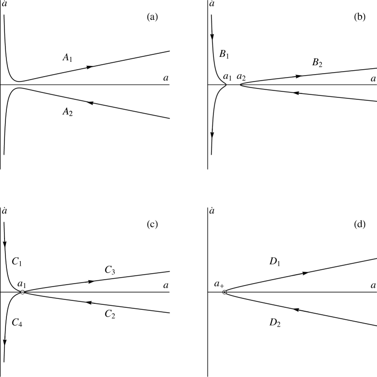
Figure 2: Trajectories in the $(a,\dot{a})$ phase space of the solutions of the classical model with constant inflaton potential given by Eq. (21) in the four possible cases: (a) $(4/27)a_{+}^{4}<b_{+}$; (b) $0<b_{+}<(4/27)a_{+}^{4}$; (c) $b_{+}=(4/27)a_{+}^{4}$; and (d) $b_{+}=0$.

We consider inflaton models with a constant potential as their solutions exhibit one or both periods of kinetic dominance and of inflationary expansion. These models are relevant on the domain of interest of models with slowly-varying potentials around a value $\phi_{0}$, where the potential may be approximated by a constant $V_{0}$,

$$V(\phi)\approx V(\phi_{0})=V_{0},$$ (19)

For example, the Starobinski model with potential $V(\phi)=\Lambda^{2}[1-\exp(-\sqrt{2/3}\phi/{M_{\rm pl}})]^{2}$ is slowly-varying around any large value of $\Phi$, where $V(\phi)\approx\Lambda^{2}$.

For a constant potential Eq (2) reduces to

$$\dot{\phi}(t)a(t)^{3}=\dot{\phi}(t_{0})a(t_{0})^{3},$$ (20)

where $t_{0}$ is a given value of the cosmic time, and Eq. (3) can be written as

$$\dot{a}^{2}=\frac{a^{2}}{a_{+}^{2}}+\frac{b_{+}}{a^{4}}-1,$$ (21)

where

$$a_{+}=M_{\rm pl}\sqrt{3/V_{0}},$$ (22)

and

$$b_{+}=\frac{(\dot{\phi}(t_{0})a(t_{0})^{3})^{2}}{6{M_{\rm pl}}^{2}}.$$ (23)

Equation (21) can be solved by separation of variables,

$$t-t_{0}=\pm\int_{a(t_{0})}^{a(t)}\frac{da}{\sqrt{\frac{a^{2}}{a_{+}^{2}}+\frac{b_{+}}{a^{4}}-1}}.$$ (24)

These solutions can be classified into four types depending on the number of zeros of the right-hand side of Eq. (21) on the domain $a>0$. For convenience, in the following discussion we denote this right-hand side by $f(a)$, i.e., $f(a)=a^{2}/a_{+}^{2}+b_{+}/a^{4}-1$.

• If $(4/27)a_{+}^{4}<b_{+}$, then there are no zeros of $f(a)$ in the domain $a>0$, and the solutions give rise to the two families of trajectories in the $(a,\dot{a})$ phase map shown in Fig. 2(a). The upper trajectory $A_{1}$ describes an expanding universe starting from a KD stage near a singularity $a=0$ at cosmic time

  $$t^{*}=t_{0}+\int_{a(t_{0})}^{0}\frac{da}{\sqrt{\frac{a^{2}}{a_{+}^{2}}+\frac{b_{+}}{a^{4}}-1}},$$ (25)

  such that $\dot{a}$ first decreases towards a positive minimum value at

  $$a_{\text{in}}=(2b_{+})^{1/6}\,a_{+}^{1/3},$$ (26)

  an then enters an unlimited period of inflationary expansion. The solutions giving rise to the trajectory $A_{2}$ describe the corresponding contracting, time-reversed evolution.

• If $0<b_{+}<(4/27)a_{+}^{4}$, then $f(a)$ has two positive zeros $0<a_{1}<a_{2}$,

  $$a_{k}=a_{+}\sqrt{\frac{1}{3}+\frac{2}{3}\cos\left(\frac{1}{3}\arccos\left(1-\frac{27\,b_{+}}{2\,a_{+}^{4}}\right)-(k-1)\frac{2\pi}{3}\right)},\quad k=1,2,$$ (27)

  and there are the two classes of trajectories shown in Fig. 2(b). The trajectory $B_{1}$ represents solutions with $a\leq a_{1}$ that describe universes which expand from a KD stage near a singularity $a=0$ until they reach a maximum $a(t)=a_{1}$, and then contract towards another KD stage near $a=0$. These solutions do not have an INF period. The trajectory $B_{2}$ represents solutions with $a\geq a_{2}$ which describe universes without any KD period: they contract until they bounce at $a=a_{2}$ and begin a period of unlimited INF expansion.

• If $b_{+}=(4/27)a_{+}^{4}$, $f(a)$ has a unique positive zero at

  $$a_{0}=\sqrt{\frac{2}{3}}\,a_{+},$$ (28)

  but $f(a)\geq 0$ for $a>0$. The corresponding trajectories are shown in Fig. 2(c), which includes the constant solution $a=a_{0}$ as well as four families of trajectories, two of which ($C_{1}$ and $C_{2}$) tend asymptotically to $a_{0}$ in the future, and the other two ($C_{3}$ and $C_{4}$) in the past.

• Finally, if $b_{+}=0$, then $f(a)$ has a unique positive zero at $a=a_{+}$, but $f(a)\geq 0$ only for $a\geq a_{+}$. The corresponding trajectories are shown in Fig. 2(d), which features the constant solutions $a=a_{+}$ as well as two families of solutions ($D_{1}$, expanding, and $D_{2}$, contracting), without KD periods, and which tend asymptotically to $a_{+}$ in the past and in the future, respectively. The solutions corresponding to $D_{1}$ are in an unlimited period of INF expansion. The particular case $a(t_{0})=a_{+}$ can be explicitly integrated to give the de Sitter form,

  $$a(t)=a_{+}\cosh\left(\frac{1}{a_{+}}(t-t_{0})\right).$$ (29)

III The WDW equation and its WKB solutions

In this Section we briefly recall the derivation of the WDW equation, the structure of its WKB solutions, and the relation of the latter to the classical inflaton Eqs. (2)–(3). This relation will be particularized in the following Section to the case of a constant inflaton potential, which in turn will be used to discuss possible types of emerging universes.

III.1 The WDW equation

The momenta conjugate to the variables $a$ and $\phi$ in the Hamiltonian formulation of the inflaton model turn out to be [11]

$$P_{a}=-12\pi^{2}{M_{\rm pl}}^{2}a\dot{a},$$ (30)

and

$$P_{\phi}=2\pi^{2}a^{3}\dot{\phi},$$ (31)

respectively. If we substitute these values in Eq. (3) rewritten in the form

$$6{M_{\rm pl}}^{2}a\,\dot{a}^{2}-a^{3}\,\dot{\phi}^{2}+6{M_{\rm pl}}^{2}\,\left(a-\frac{V(\phi)}{3{M_{\rm pl}}^{2}}a^{3}\right)=0,$$ (32)

we arrive at

$$P_{a}^{2}-\frac{6{M_{\rm pl}}^{2}}{a^{2}}\,P_{\phi}^{2}+U(a,\phi)=0,$$ (33)

where $U(a,\phi)$ is the superpotential function

$$U(a,\phi)=\frac{1}{\lambda^{2}}\left(a^{2}-\frac{V(\phi)}{3{M_{\rm pl}}^{2}}a^{4}\right),$$ (34)

and where

$$\lambda=\frac{1}{12\pi^{2}{M_{\rm pl}}^{2}}.$$ (35)

Incidentally, since the left-hand side of Eq. (33) is proportional to $a\mathcal{H}$, where $\mathcal{H}$ is the Hamiltonian of the inflaton model [11], Eq. (33) shows that the solutions of Eqs. (2)–(3) satisfy the zero-energy constraint $\mathcal{H}=0$.

Quantization is performed by the rules,

$$P_{a}\rightarrow-i\,\hbar\frac{\partial}{\partial a},\quad P_{\phi}\rightarrow-i\,\hbar\frac{\partial}{\partial\phi},$$ (36)

with the proviso of an ambiguity in the ordering of $a$ and $\partial/\partial a$ in the quantization of $P_{a}^{2}$, which in effect leads to the quantization rule

$$P_{a}^{2}\rightarrow-\hbar^{2}\frac{1}{a^{p}}\frac{\partial}{\partial a}a^{p}\frac{\partial}{\partial a},$$ (37)

where $p$ is an (in principle) arbitrary parameter. Thus we arrive at the celebrated WDW equation [29],

$$\left(\frac{\partial^{2}}{\partial a^{2}}+\frac{p}{a}\frac{\partial}{\partial a}-\frac{6{M_{\rm pl}}^{2}}{a^{2}}\frac{\partial^{2}}{\partial\phi^{2}}-\frac{1}{\hbar^{2}}U(a,\phi)\right)\Psi(a,\phi)=0.$$ (38)

III.2 General remarks on the WKB solutions of the WDW equation

WKB solutions of Eq. (38) have the usual exponential form

$$\Psi(a,\phi)=\exp\left(i\,\mathbb{S}(a,\phi)/\hbar\right),$$ (39)

where $\mathbb{S}$ is expanded as an asymptotic power series in $\hbar$,

$$\mathbb{S}=\mathbb{S}_{0}+\frac{\hbar}{i}\mathbb{S}_{1}+\left(\frac{\hbar}{i}\right)^{2}\mathbb{S}_{2}+\cdots,\quad\hbar\rightarrow 0.$$ (40)

By substituting Eqs. (39)–(40) into the WDW Eq. (38) and setting to zero terms with the same power of $\hbar$ we obtain a sequence of two-dimensional WKB equations for the $\mathbb{S}_{n}$, which have to be solved recursively.

The first equation, for $\mathbb{S}_{0}$, is the Hamilton-Jacobi equation,

$$\left(\frac{\partial\mathbb{S}_{0}}{\partial a}\right)^{2}-\frac{1}{2\pi^{2}\lambda a^{2}}\left(\frac{\partial\mathbb{S}_{0}}{\partial\phi}\right)^{2}+U=0,$$ (41)

and the second equation, for $\mathbb{S}_{1}$, is

$$\frac{\partial^{2}\mathbb{S}_{0}}{\partial a^{2}}-\frac{6{M_{\rm pl}}^{2}}{a^{2}}\frac{\partial^{2}\mathbb{S}_{0}}{\partial\phi^{2}}+2\frac{\partial\mathbb{S}_{0}}{\partial a}\frac{\partial\mathbb{S}_{1}}{\partial a}-\frac{12{M_{\rm pl}}^{2}}{a^{2}}\frac{\partial\mathbb{S}_{0}}{\partial\phi}\frac{\partial\mathbb{S}_{1}}{\partial\phi}+\frac{p}{a}\frac{\partial\mathbb{S}_{0}}{\partial a}=0.$$ (42)

Note that the Hamilton-Jacobi Eq. (41) does not depend on the ordering parameter $p$, while Eq. (42) does.

WKB solutions of the WDW equation in the classically allowed regions are oscillatory, and these are the regions where the nucleation of classical universes with specific properties may emerge [13, 31]. We also recall that the potential $V(\phi)$ must be positive and smaller than the Planck density ${M_{\rm pl}}^{4}$ for the semiclassical solutions obtained from Eqs. (41)–(42) to be valid [10]. The identification between the classical momenta as defined in Eqs. (30)–(31) and the corresponding derivatives of $\mathbb{S}_{0}$,

$$P_{a}=\frac{\partial\mathbb{S}_{0}}{\partial a},\quad P_{\phi}=\frac{\partial\mathbb{S}_{0}}{\partial\phi},$$ (43)

leads to the system of first-order differential equations,

$$\dot{a}=-\frac{\lambda}{a}\frac{\partial\mathbb{S}_{0}}{\partial a},\quad\dot{\phi}=\frac{1}{2\pi^{2}a^{3}}\frac{\partial\mathbb{S}_{0}}{\partial\phi}.$$ (44)

Thus, each solution of Eq. (41) corresponds to a biparametric (the initial conditions for $a$ and $\phi$) family of solutions of Eqs. (2)–(3), and this family in turn characterizes the properties of the emergent classical universes in the classically allowed regions. It is then said [13, 31] that the wavefunction $\Psi(a,\phi)$ is peaked about the associated solutions of the system (44).

IV THE WDW EQUATION WITH A CONSTANT POTENTIAL

In this Section we look for solutions of the WDW equation with a constant potential using the ansatz

$$\Psi(k,a,\phi)=\psi(k,a)e^{ik\phi/\hbar},$$ (45)

where $k$ is a real parameter. Variables in the WDW equation separate and we get the following equation for $\psi(k,a)$,

$$\left(\frac{d^{2}}{da^{2}}+\frac{p}{a}\frac{d}{da}-\hbar^{-2}\mathrm{U}(k,a)\right)\psi(k,a)=0,$$ (46)

where

$$\mathrm{U}(k,a)=-\frac{6{M_{\rm pl}}^{2}k^{2}}{a^{2}}+U(a,\phi_{0})=-\frac{6{M_{\rm pl}}^{2}k^{2}}{a^{2}}+\frac{a^{2}}{\lambda^{2}}\left(1-\frac{a^{2}}{a_{+}^{2}}\right).$$ (47)

The first term in the modified superpotential $\mathrm{U}(k,a)$ is a consequence of the phase factor $\exp(ik\phi/\hbar)$ in the wavefunction ansatz Eq. (45), and induces a dependence of the solutions of the WDW equation on the scale factor different from those in Refs. [11, 31]. This term is dominant as $a\to 0^{+}$, and in the next Sections we will discuss its effect on the overall behavior of the WKB solutions via connection formulas.

IV.1 WKB solutions

The actions $\mathbb{S}$ and $S$ of the WKB solutions for $\Psi(k,a,\phi)$ and

$$\psi(k,a)=e^{iS(k,a)/\hbar},$$ (48)

in Eq. (45) are related by $\mathbb{S}=S+k\phi$, which after expansion in powers of $\hbar$ leads to $\mathbb{S}_{0}=S_{0}+k\phi$ and $\mathbb{S}_{n}=S_{n}$ for $n\geq 1$ (with $S_{n}$ independent of $\phi$). Therefore, the classical system Eq. (44) on whose solutions the wavefunctions $\Psi(k,a,\phi)$ are strongly peaked is,

$$\dot{a}^{2}=-\frac{\lambda^{2}}{a^{2}}\mathrm{U}(k,a),\quad\dot{\phi}=\frac{k}{2\pi^{2}a^{3}},$$ (49)

which using Eq. (47) reduces to Eqs. (20)–(21) with

$$b_{+}=\frac{k^{2}}{24\pi^{4}{M_{\rm pl}}^{2}}.$$ (50)

Likewise, Eqs. (41) and (42) reduce to equations for $S_{0}$ and $S_{1}$,

$$\left(\frac{dS_{0}}{da}\right)^{2}+\mathrm{U}(k,a)=0,$$ (51)

$$\frac{d^{2}S_{0}}{da^{2}}+2\frac{dS_{0}}{da}\frac{dS_{1}}{da}+\frac{p}{a}\frac{dS_{0}}{da}=0,$$ (52)

which can be readily solved. On the classically allowed regions $\mathrm{U}(k,a)<0$ we find

$$S_{0}(k,a)=\int_{a_{r}}^{a}\mathrm{p}(k,a^{\prime})da^{\prime},$$ (53)

where

$$\mathrm{p}(k,a)=\left(-\mathrm{U}(k,a)\right)^{1/2},$$ (54)

$a_{r}$ is an appropriate reference point, and

$$S_{1}(k,a)=-\frac{1}{2}\log(a^{p}\mathrm{p}(k,a)).$$ (55)

Therefore, the basic WKB solutions of Eq. (46) on the classically allowed regions are

$$\psi_{\pm}(k,a)=\frac{1}{(a^{p}\mathrm{p}(k,a))^{1/2}}\exp\left(\pm\frac{i}{\hbar}\int_{a_{r}}^{a}\mathrm{p}(k,a^{\prime})da^{\prime}\right).$$ (56)

Eq. (47) shows that for $k\neq 0$ the modified superpotential $\mathrm{U}(k,a)$ is strictly negative both for large and small values of $a>0$, and therefore these regions are classically allowed regions for nonvanishing values of $k$, values to which we restrict hereafter. The classical system Eq. (44) on whose solutions the wavefunctions $\psi$ are strongly peaked is

$$\dot{a}=\mp\frac{\lambda}{a}\mathrm{p}(k,a),\quad\dot{\phi}=\frac{k}{2\pi^{2}a^{3}},$$ (57)

which reduces to Eqs. (20)–(21) with $b_{+}$ defined in Eq. (50). Note in particular that the first equation of this system shows that $\psi_{+}$ and $\psi_{-}$ describe contracting and expanding universes, respectively.

IV.2 Leading behavior of the WKB solutions at large scale factor

As we mentioned earlier, at large $a$ we may neglect the $k$-dependent term in the modified superpotential Eq. (47),

$$\mathrm{U}(k,a)\sim U_{+}(a)=\frac{a^{2}}{\lambda^{2}}\left(1-\frac{a^{2}}{a_{+}^{2}}\right),\quad\mbox{ as }a\to\infty,$$ (58)

in effect recovering the well-known model for studying the emergence of inflation from the WDW equation discussed, e.g., in Refs. [11, 31],

$$\left(\frac{d^{2}}{da^{2}}+\frac{p}{a}\frac{d}{da}-\hbar^{-2}U_{+}(a)\right)\psi^{(\infty)}(a)=0.$$ (59)

Since in our case $k\neq 0$ these results apply only to large $a$, we have labeled the wavefunction as $\psi^{(\infty)}(a)$. We summarize here the relevant notations and results.

The generic shape of the superpotential $U_{+}(a)$ in shown in Fig. 3, and corresponds to a quantum tunneling problem with a classically forbidden region $0<a<a_{+}$ and a classically allowed region $a>a_{+}$.

Figure 3: Generic shape of the superpotential $U_{+}(a)$ defined in Eq. (58).

Since $a_{+}$ is the unique positive zero of $U_{+}(a)$, it is natural to take it as the reference point for the WKB solutions. By using Eq. (56) with $\mathrm{U}(k,a)$ replaced by $U_{+}(a)$ and $a_{r}=a_{+}$, we obtain the following ($k$-independent) approximations $\psi_{\pm}^{(\infty)}(a)$ to the ($k$-dependent) functions $\psi_{\pm}(k,a)$ valid for large $a$,

$$\psi_{\pm}^{(\infty)}(a)=\lambda^{1/2}a^{-p/2}\left(\frac{a^{4}}{a_{+}^{2}}-a^{2}\right)^{-1/4}\exp\left[\pm\frac{i}{\hbar}\,\frac{{M_{\rm pl}}^{2}}{\lambda V_{0}}\left(\frac{a^{2}}{a_{+}^{2}}-1\right)^{3/2}\right],\quad a_{+}<a.$$ (60)

The wavefunctions $\psi_{+}^{(\infty)}(a)$ and $\psi_{-}^{(\infty)}(a)$ represent contracting and expanding universes in the inflationary period, respectively.

Two distinguished wavefunctions are usually defined in terms of the $\psi_{\pm}^{(\infty)}(a)$. The Vilenkin tunneling wavefunction $\psi_{\mathrm{T}}(a)$ is defined as [11, 31],

$$\psi_{\mathrm{T}}(a>a_{+})=e^{i\pi/4}A\psi_{-}^{(\infty)}(a),$$ (61)

where

$$A=e^{-{M_{\rm pl}}^{2}/(\hbar\lambda V_{0})}.$$ (62)

The function $\psi_{\mathrm{T}}(a)$ represents an expanding universe in the region $a>a_{+}$, and the corresponding complete wavefunction in that region is

$$\Psi_{\mathrm{T}}(k,a,\phi)=\psi_{\mathrm{T}}(a)e^{ik\phi/\hbar}.$$ (63)

Likewise, the Hartle-Hawking no-boundary wavefunction [8, 9] is defined by the following superposition of wavefunctions representing contracting and expanding universes,

$$\psi_{\mathrm{NB}}(a>a_{+})=A^{-1}(e^{-i\pi/4}\psi_{+}^{(\infty)}(a)+e^{+i\pi/4}\psi_{-}^{(\infty)}(a)),$$ (64)

and the corresponding complete wavefunction is

$$\Psi_{\mathrm{NB}}(k,a,\phi)=\psi_{\mathrm{NB}}(a)e^{ik\phi/\hbar}.$$ (65)

Note that if $V_{0}\ll{M_{\rm pl}}^{4}$, then $a_{+}$ is much larger than the classical lower limit for the scale factor given by Eq. (8),

$$a_{+}\gg\frac{\sqrt{3}}{{M_{\rm pl}}},$$ (66)

and from Eq. (12) it follows that during the classical inflation regime

$$a>\sqrt{\frac{2}{3}}a_{+}.$$ (67)

Therefore, $a_{+}$ is an appropriate lower limit for a classical inflationary stage.

IV.3 Leading behavior of the WKB solutions at small scale factor

For $a$ near zero we neglect the term proportional to $a^{4}$ in $\mathrm{U}(k,a)$,

$$\mathrm{U}(k,a)\sim U_{-}(k,a)=\frac{a^{2}}{\lambda^{2}}\left(1-\frac{a_{-}(k)^{4}}{a^{4}}\right),\quad\mbox{ as }a\to 0^{+},$$ (68)

where

$$a_{-}(k)=(\sqrt{6}{M_{\rm pl}}\lambda|k|)^{1/2},$$ (69)

is the unique positive zero of $U_{-}(k,a)$. The superpotential $U_{-}(k,a)$, illustrated in Fig. 4, corresponds to quantum tunneling between the classically allowed region $0<a<a_{-}(k)$ and the classically forbidden region $a_{-}(k)<a$, The analog of Eq. (59) is

$$\left(\frac{d^{2}}{da^{2}}+\frac{p}{a}\frac{d}{da}-\frac{1}{\hbar^{2}}U_{-}(k,a)\right)\psi^{(0)}(k,a)=0.$$ (70)

Figure 4: Generic shape of the superpotential $U_{-}(k,a)$ (with $k\neq 0$) defined in Eqs. (68)–(69).

Again, since $a_{-}(k)$ is the unique positive zero of $U_{-}(k,a)$, it is natural to take it as the reference point for the WKB solutions. By using Eq. (56) with $\mathrm{U}(k,a)$ replaced by $U_{-}(k,a)$ and $a_{r}=a_{-}(k)$, we obtain the following approximations $\psi_{\pm}^{(0)}(k,a)$ to the functions $\psi_{\pm}(k,a)$ valid for small $a$,

$$\psi_{\pm}^{(0)}(k,a)=\lambda^{1/2}a^{-\frac{p+1}{2}}\left(\frac{a_{-}(k)^{4}}{a^{4}}-1\right)^{-1/4}\exp\left(\pm\frac{i}{\hbar}\int_{a_{-}(k)}^{a}\mathrm{p}_{-}(k,a^{\prime})da^{\prime}\right),$$ (71)

where

$$\int_{a_{-}(k)}^{a}\mathrm{p}_{-}(k,a^{\prime})da^{\prime} = \frac{1}{2\lambda}\left[\sqrt{a_{-}(k)^{4}-a^{4}}+a_{-}(k)^{2}\log a^{2}\right.$$ (72)

$$\qquad{}\left.-a_{-}(k)^{2}\log\left(a_{-}(k)^{2}+\sqrt{a_{-}(k)^{4}-a^{4}}\right)\right].$$

Since for $a\ll a_{-}(k)$

$$\int_{a_{-}(k)}^{a}\mathrm{p}_{-}(k,a^{\prime})da^{\prime}\sim\frac{a_{-}(k)^{2}}{\lambda}\log a,$$ (73)

Eq. (71) implies

$$\psi_{\pm}^{(0)}(k,a)\sim\frac{\lambda^{1/2}}{a_{-}(k)}a^{(1-p)/2}\exp\left(\pm\frac{i}{\hbar}\sqrt{6}\,M_{\rm pl}|k|\log a\right),\quad a\ll a_{-}(k).$$ (74)

Thus the complete wavefunctions can be approximated as

$$\Psi_{\pm}^{(0)}(k,a,\phi)\sim\frac{\lambda^{1/2}}{a_{-}(k)}a^{2\nu}\exp\left[\pm\frac{i}{\hbar}(\sqrt{6}\,M_{\rm pl}|k|\log a\pm k\phi)\right],\quad a\ll a_{-}(k),$$ (75)

where $\nu=(1-p)/4$. The admissible wavefunctions should be regular at $a=0$ and this is satisfied only if $\nu\geq 0$ or, equivalently, if $p\leq 1$.

The wavefronts of these approximations are given by the classical trajectories of $(a,\phi)$ in the KD period,

$$\sqrt{6}\,M_{\rm pl}\log a\pm\phi=const,$$ (76)

and the wavefunctions $\Psi_{+}^{(0)}(k,a,\phi)$ and $\Psi_{-}^{(0)}(k,a,\phi)$ represent contracting and expanding universes in the KD period, respectively.

Finally, taking into account Eq. (35), from Eq. (69) we find that

$$a_{-}^{2}=\frac{|k|}{2\sqrt{6}\pi^{2}M_{\rm pl}}.$$ (77)

Therefore, $a_{-}$ satisfies the classical limit condition Eq. (8) for the scale factor if

$$|k|>\frac{6\sqrt{6}\pi^{2}}{M_{\rm pl}}.$$ (78)

V TYPES OF EMERGENT UNIVERSES

In this Section we will describe the different types of classical universes which may emerge from the solutions Eq. (45) of the WDW equation with a constant potential.

V.1 Type-$A$ universes

Classical universes evolving according to solutions of type $A_{1}$ (expanding) and $A_{2}$ (contracting) of Eqs. (20)–(21) with both KD and INF periods arise provided that $(4/27)a_{+}^{4}<b_{+}$, which restated in terms of the parameters appearing in the corresponding semiclassical wavefunctions is equivalent to (see Eq. (50)),

$$k^{2}>32\pi^{4}\frac{{M_{\rm pl}}^{6}}{V_{0}^{2}}.$$ (79)

In this case $\mathrm{U}(k,a)$ is strictly negative on the domain $a>0$, and the wavefunctions

$$\Psi_{\pm}(k,a,\phi)=\psi_{\pm}(k,a)e^{ik\phi/\hbar},$$ (80)

where

$$\psi_{\pm}(k,a)=\frac{1}{(a^{p}\mathrm{p}(k,a))^{1/2}}\exp\left(\pm\frac{i}{\hbar}\int_{a_{+}}^{a}\mathrm{p}(k,a^{\prime})da^{\prime}\right),$$ (81)

are well-defined oscillatory functions on the whole classically allowed domain $a>0$.

In Sec. IV-B we showed that for large $a$ the function $\Psi_{-}(k,a,\phi)$ describes expanding INF universes. If we factorize $\psi_{-}(k,a)$ in the form

$$\psi_{-}(k,a)=\frac{1}{(a^{p}\mathrm{p}(k,a))^{1/2}}\exp\left(-\frac{i}{\hbar}\int_{a_{+}}^{a_{-}(k)}\mathrm{p}(k,a^{\prime})da^{\prime}\right)\exp\left(-\frac{i}{\hbar}\int_{a_{-}(k)}^{a}\mathrm{p}(k,a^{\prime})da^{\prime}\right),$$ (82)

we see that near $a=0$ the last factor behaves as $\psi_{-}^{(0)}(k,a)$ and, from the analysis of Sec. IV-C, in this small $a$ region $\Psi_{-}(k,a,\phi)$ describes expanding universes in the KD regime. Therefore $\Psi_{-}(k,a,\phi)$ is indeed peaked about a type-$A_{1}$ solution.

A similar argument shows that $\Psi_{+}(k,a,\phi)$ is peaked about a type-$A_{2}$ solution.

V.2 Type-$B$ universes

Classical universes evolving according to solutions of type $B_{1}$ or $B_{2}$ of Eqs. (20)–(21) arise if $0<b_{+}<(4/27)a_{+}^{4}$, or, equivalently,

$$0<k^{2}<32\pi^{4}\frac{{M_{\rm pl}}^{6}}{V_{0}^{2}}.$$ (83)

In this case $\mathrm{U}(k,a)$ has two positive zeros $0<a_{1}<a_{2}$ given by Eq. (27), and corresponds to the potential barrier illustrated in Fig. 5.

Figure 5: Generic shape of the superpotential $\mathrm{U}(k,a)$ for $0<k^{2}<32\pi^{4}{M_{\rm pl}}^{6}/V_{0}^{2}$ with the two classically allowed regions $0<a<a_{1}$ and $a_{2}<a$.

There are two classically allowed regions, $0<a<a_{1}$ and $a_{2}<a$, with respective basic WKB wavefunctions given by,

$$\psi_{\pm}^{(r)}(k,a)=\frac{1}{(a^{p}\mathrm{p}(k,a))^{1/2}}\exp\left(\pm\frac{i}{\hbar}\int_{a_{r}}^{a}\mathrm{p}(k,a^{\prime})da^{\prime}\right),\quad r=1,2,$$ (84)

which in turn can be approximated by $\psi_{\pm}^{(0)}(k,a)$ and $\psi_{\pm}^{(\infty)}(a)$ for $r=1$ and $r=2$ respectively.

Using the standard WKB connection formulas (wherein the semiclassical expansions are interpreted as asymptotic expansions in the sense of Poincaré) to connect these two sets of WKB solutions across the barrier leads to a well-known loss of unitarity [33, 34]. To circumvent this problem, we interpret the asymptotic expansions in the sense of Borel, and use the ensuing connections formulas of Silverstone [35]. Since the classically forbidden region is a Stokes line, it is necessary to “pick sides,” and we choose to take $\mathrm{Im}\,a\to 0^{+}$. The calculation is strictly analogous to the calculation corresponding to the piecewise linear potential in Fig. 1(b) of Ref. [36], where all the intermediate steps are carried out in detail. Thus we find,

$$\psi_{+}^{(2)}(k,a)\rightarrow e^{K(k)}(\psi_{+}^{(1)}(k,a)-i\psi_{-}^{(1)}(k,a)),$$ (85)

$$\psi_{-}^{(2)}(k,a)\rightarrow e^{K(k)}(\psi_{-}^{(1)}(k,a)+i\,\psi_{+}^{(1)}(k,a))-ie^{-K(k)}\psi_{+}^{(1)}(k,a),$$ (86)

and, conversely,

$$\psi_{+}^{(1)}(k,a)\rightarrow e^{K(k)}(\psi_{+}^{(2)}(k,a)+i\psi_{-}^{(2)}(k,a)),$$ (87)

$$\psi_{-}^{(1)}(k,a)\rightarrow e^{K(k)}(\psi_{-}^{(2)}(k,a)-i\psi_{+}^{(2)}(k,a))+ie^{-K(k)}\psi_{+}^{(2)}(k,a),$$ (88)

where

$$K(k)=\frac{1}{\hbar}\int_{a_{1}}^{a_{2}}|\mathrm{p}(k,a)|\,da.$$ (89)

As a consequence it follows that

$$\psi_{+}^{(1)}(k,a)-i\psi_{-}^{(1)}(k,a)\rightarrow e^{-K(k)}\psi_{+}^{(2)}(k,a),$$ (90)

and

$$\psi_{+}^{(2)}(k,a)+i\psi_{-}^{(2)}(k,a)\rightarrow e^{-K(k)}\psi_{+}^{(1)}(k,a).$$ (91)

(The standard WKB connection formulas would have led to Eqs. (90) and (91) with their right-hand sides equal to zero, with the apparent result that a nonzero oscillatory wavefunction at one side of the barrier connects to a zero wavefunction on the other side of the barrier. These connection formulas do not capture the physically intuitive result that the wavefunction on the other side of the barrier is also oscillatory but suppressed by an exponentially small factor of the order of $\exp(-K(k))$.)

Therefore, the wavefunction corresponding to the WKB approximation given by

$$\Psi^{(1)}(k,a,\phi)=\left(\psi_{+}^{(1)}(k,a)-i\psi_{-}^{(1)}(k,a)\right)e^{ik\phi/\hbar},\quad 0<a<a_{1},$$ (92)

is a superposition of an expanding component and a contracting component peaked about classical solutions of Eqs. (20)–(21) in a KD period. In addition, this WKB wavefunction is suppressed by an exponentially small factor for $a>a_{2}$ and, consequently, $\Psi^{(1)}(k,a,\phi)$ is peaked about $B_{1}$ solutions of Eqs. (20)–(21).

Likewise, the wavefunction corresponding to the WKB approximation

$$\Psi^{(2)}(k,a,\phi)=\left(\psi_{+}^{(2)}(k,a)+i\psi_{-}^{(2)}(k,a)\right)e^{ik\phi/\hbar},\quad a_{2}<a<\infty,$$ (93)

is a superposition of expanding and contracting components peaked about classical solutions of Eqs. (20)–(21) in an inflationary period, and is suppressed by an exponentially small factor for $0<a<a_{1}$ . Therefore $\Psi^{(2)}(k,a,\phi)$ is peaked about the $B_{2}$ type solutions of Eqs. (20)–(21). Note that for large $a$ the no-boundary wavefunction $\psi_{\mathrm{NB}}(k,a,\phi)$ and $\Psi^{(2)}(k,a,\phi)$ are related by

$$\Psi_{\mathrm{NB}}(k,a,\phi)=A^{-1}e^{-i\pi/4}\Psi^{(2)}(k,a,\phi).$$ (94)

V.3 Type-$C$ and type-$D$ universes

Type-$C$ universes emerge as semiclassical limits of wavefunctions for $k^{2}=32\pi^{4}{M_{\rm pl}}^{6}/V_{0}^{2}$, and are limiting cases of type-$B$ universes as $a_{1}\rightarrow a_{2}$.

Finally, type-$D$ universes are associated with wavefunctions with $k=0$, and are the same as those studied in Ref. [11]. The subtype $D_{1}$ describes expanding inflationary universes without a KD period and corresponds to $\psi_{-}^{(\infty)}(a)$ wavefunctions in Eq. (60). Subtype $D_{2}$ describes contracting universes without a KD period and corresponds to wavefunctions $\psi_{+}^{(\infty)}(a)$ in Eq. (60).

VI PROBABILITY DISTRIBUTIONS

The probabilistic interpretation of the solutions of the WDW equation is formulated in terms of the components of the current [29, 10, 11, 31]

$$j^{a}=\frac{i}{2}\hbar\,a^{p}(\Psi^{*}\partial_{a}\Psi-\Psi\partial_{a}\Psi^{*}),$$ (95)

$$j^{\phi}=-i\,3{M_{\rm pl}}^{2}\,\hbar\,a^{p-2}(\Psi^{*}\partial_{\phi}\Psi-\Psi\partial_{\phi}\Psi^{*}),$$ (96)

which satisfy the continuity equation

$$\partial_{a}j^{a}+\partial_{\phi}j^{\phi}=0.$$ (97)

In general, these components are not positive definite and their interpretation requires the analysis of an appropriate time variable [10, 11]. If $a$ is taken as a time variable, then $\rho_{\phi_{0}}(a)=j^{a}$ is interpreted as the probability density for $\phi=\phi_{0}$ at a given value of $a$. The quantity $\partial_{\phi}j^{\phi}$ for the solutions $\Psi(k,a,\phi)$ of the form of Eq. (45) vanishes identically and, consequently, the density $\rho_{\phi_{0}}(a)$ is $a$-independent. It turns out that the $\rho_{\phi_{0}}(a)$ for a generic WKB wavefunction of the WDW equation is positive (negative) if the wavefunction corresponds to expanding (contracting) universes [10].

Let us consider the expanding universes with an inflationary period $A_{1},B_{2},C_{3}$ and $D_{1}$. Their wavefunctions for large $a$ are approximated by $\psi_{-}^{(\infty)}(a)$, and from Eq. (56) it follows that

$$\psi_{-}^{(\infty)*}\partial_{a}\psi_{-}^{(\infty)}-\psi_{-}^{(\infty)}\partial_{a}\psi_{-}^{(\infty)*}=-\frac{2i}{\hbar a^{p}},$$ (98)

which leads to a constant density

$$\rho_{\phi_{0}}(a)=1.$$ (99)

As a consequence of Eq. (99), Vilenkin’s tunneling wavefunction $\psi_{\mathrm{T}}$ on the region $a>a_{+}$ satisfies

$$\rho_{T,\phi_{0}}(a)=\exp{\left(-\frac{24\pi^{2}{M_{\rm pl}}^{4}}{\hbar V(\phi_{0})}\right)}=\exp{\left(-\frac{2}{3\mathbb{V}(\phi_{0})}\right)},$$ (100)

where $\mathbb{V}=\hbar V/(6\pi{M_{\rm pl}}^{2})^{2}$ is the potential function with the Vilenkin normalization (see Eq. (4.15) in Ref. [11]). This expression is the standard result for the probability density for the Vilenkin tunneling function [11, 31].

Of the four types of universes $A_{1},B_{2},C_{3}$ and $D_{1}$ under consideration, only the type $A_{1}$ has a KD period in addition to the inflationary period. Moreover, from Eq. (82) we have that near $a=0$ the wavefunction corresponding to the $A_{1}$ type is approximated by

$$\psi_{-}(k,a)=\exp\left(-\frac{i}{\hbar}\int_{a_{+}}^{a_{-}(k)}\mathrm{p}(k,a^{\prime})da^{\prime}\right)\psi_{-}^{(0)}(k,a).$$ (101)

Then, using Eqs. (75) and (69) we obtain

$$\rho_{\phi_{0}}(a)=\frac{\lambda}{a_{-}^{2}}\sqrt{6}{M_{\rm pl}}|k|=1$$ (102)

which is the same constant density as that calculated for large $a$ in Eq. (99).

VII CONCLUSIONS

In the present work we have discussed the emergence of KD classical universes in closed Friedmann universes with unit curvature from a certain family of WKB solutions of the WDW equation with a constant inflaton potential. These WKB solutions are semiclassical approximations to eigenfunctions of the momentum operator conjugate to the inflaton, i.e., they depend on the inflaton field $\phi$ through a phase factor $\exp{i(k\phi/\hbar)}$. The standard treatment of this problem has been restricted to $k=0$, and leads to a large-$a$, classically allowed, INF region, and to a small-$a$, classically forbidden region. Allowing for $k\neq 0$ replaces this scenario with a new one, in which two classically allowed regions separated by a potential barrier via two turning points may arise. In the innermost region there are semiclassical solutions peaked about KD classical solutions, and in the outermost region we find, among others, the well-known Vilenkin tunneling and Hartle-Hawking no-boundary solutions times the $\phi$-dependent phase factor. We have also discussed how these solutions connect in our setting to superpositions of semiclassical wavefunctions in the KD regime. We have recovered within our approach the standard results on the INF region. Finally, in the Appendix we use the explicit integrability of the WDW equation near $a=0$ to provide expressions for the wavefunctions with WKB approximations on the KD regions in terms of first-kind modified Bessel functions.

Appendix A Solution of the WDW equation near $a=0$ in terms of Bessel functions

The general solution of Eq. (70) is a linear combination of the functions

$$f_{\pm}(k,a)=I_{\pm\omega(k)}(a^{2}/2\hbar\lambda)a^{2\nu},$$ (103)

where $I_{\pm\omega}$ are the first-kind modified Bessel functions  [37] and

$$\omega(k)=\frac{1}{2}\left[(2\nu)^{2}-6{M_{\rm pl}}^{2}k^{2}/\hbar^{2}\right]^{1/2}.$$ (104)

The generic shape of the real and imaginary parts of Eq. (103) are illustrated in Fig. 6. From the asymptotic formula [37]

$$I_{\omega}(x)\sim\frac{1}{\Gamma(1+\omega)}\left(\frac{x}{2}\right)^{\omega},\quad\mbox{ as }x\rightarrow 0,$$ (105)

it follows that

$$f_{\pm}(k,a)\sim C_{\pm}a^{2(\nu\pm\omega(k))},\quad\mbox{ as }a\rightarrow 0,$$ (106)

where

$$C_{\pm}=\frac{1}{\Gamma(1\pm\omega(k))(4\hbar\lambda)^{\pm\omega(k)}}.$$ (107)

A necessary condition for the validity of the WKB approximation Eq. (71) is

$$\frac{6M_{\rm pl}^{2}k^{2}}{\hbar^{2}}\gg 4\nu^{2},$$ (108)

in which case $\omega(k)$ is purely imaginary and in fact $\omega(k)\sim i\sqrt{6}M_{\rm pl}|k|/(2\hbar)$. Therefore, using Eq. (106) for functions $f_{\pm}(k,a)$ with values of $k$ satisfying Eq. (108), it follows that

$$F_{\pm}(k,a,\phi) = f_{\pm}(k,a)e^{ik\phi/\hbar}$$ (109)

$$\sim C_{\pm}a^{2\nu}\exp\left[\pm\frac{i}{\hbar}\,(\sqrt{6}\,M_{\rm pl}|k|\log a\pm k\phi)\right],\quad\mbox{ as }a\rightarrow 0.$$ (110)

Therefore, in view of Eqs. (75) and (110) it is clear that as $a\rightarrow 0$ the wavefunctions $\Psi_{\mp}^{(0)}(k,a,\phi)$ are proportional to the semiclassical expansions of the explicit functions

$$F_{\pm}(k,a,\phi)=I_{\pm\omega(k)}(a^{2}/2\hbar\lambda)a^{2\nu}e^{ik\phi/\hbar}.$$ (111)

Figure 6: The functions (a) $(2\hbar\lambda)^{\nu}\mathrm{Re}(\psi_{\pm}^{(0)}(k,a))$, and (b) $\pm(2\hbar\lambda)^{\nu}\mathrm{Im}(\psi_{\pm}^{(0)}(k,a))$ on the oscillatory region near $a=0$ for $\nu=1/6$ and $k=2\hbar/{M_{\rm pl}}$.

References

• Starobinsky [1980] A. Starobinsky, A new type of isotropic cosmological models without singularity, Phys. Lett. B 91, 99 (1980).
• Guth [1981] A. H. Guth, Inflationary universe: A possible solution to the horizon and flatness problems, Phys. Rev. D 23, 347 (1981).
• Linde [1982] A. D. Linde, A new inflationary universe scenario: A possible solution of the horizon, flatness, homogeneity, isotropy and primordial monopole problems, Phys. Lett. B 108, 389 (1982).
• Linde [1985] A. D. Linde, Initial conditions for inflation, Phys. Lett. B 162, 281 (1985).
• Mukhanov [2005] V. Mukhanov, Physical Foundations of Cosmology (Cambridge University Press, 2005).
• Baumann [2009] D. Baumann, Tasi Lectures on Inflation, arXiv:0907.5424  (2009).
• Martin [2018] J. Martin, The Theory of Inflation, in 200th Course of Enrico Fermi School of Physics: Gravitational Waves and Cosmology (2018) arXiv:1807.11075 [astro-ph.CO] .
• Hartle and Hawking [1983] J. B. Hartle and S. W. Hawking, Wave function of the universe, Phys. Rev. D 28, 2960 (1983).
• Hawking [1984] S. W. Hawking, The quantum state of the universe, Nuclear Physics B 239, 257 (1984).
• Vilenkin [1986] A. Vilenkin, Boundary conditions in quantum cosmology, Phys. Rev. D 33, 3560 (1986).
• Vilenkin [1988] A. Vilenkin, Quantum cosmology and the initial state of the universe, Phys. Rev. D 37, 888 (1988).
• Vilenkin [1994] A. Vilenkin, Approaches to quantum cosmology, Phys. Rev. D 50, 2581 (1994).
• Atkatz [1994] D. Atkatz, Quantum cosmology for pedestrians, Am. J. Phys. 62, 619 (1994).
• Linde [2008] A. Linde, Inflationary cosmology, in Inflationary Cosmology, Lecture Notes in Physics, Vol. 738 (Springer, 2008) pp. 1–54.
• Handley et al. [2014] W. Handley, S. Brechet, A. Lasenby, and M. P. Hobson, Kinetic initial conditions for inflation, Phys. Rev. D 89, 063505 (2014).
• Handley et al. [2019] W. Handley, A. Lasenby, and M. Hobson, Kinetically dominated curved universes: Logolinear series expansions, Phys. Rev. D 99, 123512 (2019).
• Haddadin and Handley [2018] W. I. J. Haddadin and W. J. Handley, Rapid numerical solutions for the Mukhanov-Sazaki equation, arXiv:1809.11095  (2018).
• Hergt et al. [2019] L. Hergt, W. Handley, M. Hobson, and A. Lasenby, Constraining the kinetically dominated universe, Phys. Rev. D 100, 023501 (2019).
• Medina and Martínez Alonso [2020] E. Medina and L. Martínez Alonso, Kinetic dominance and psi series in the Hamilton-Jacobi formulation of inflaton models, Phys. Rev. D 102, 103517 (2020).
• Steinhardt and Turner [1984] P. J. Steinhardt and M. S. Turner, Prescription for successful new inflation, Phys. Rev. D 29, 2162 (1984).
• Stewart and Lyth [1993] E. D. Stewart and D. H. Lyth, A more accurate analytic calculation of the spectrum of cosmological perturbations produced during inflation, Phys. Lett. B 302, 171 (1993).
• Liddle et al. [1994] A. R. Liddle, P. Parsons, and J. D. Barrow, Formalizing the slow-roll approximation in inflation, Phys. Rev. D 50, 7222 (1994).
• Lidsey et al. [1997] J. E. Lidsey, A. R. Liddle, E. W. Kolb, E. J. Copeland, T. Barreiro, and M. Abney, Reconstructing the inflaton potential—an overview, Rev. Mod. Phys. 69, 373 (1997).
• Bassett et al. [2006] B. A. Bassett, S. Tsujikawa, and D. Wands, Inflation dynamics and reheating, Rev. Mod. Phys. 78, 537 (2006).
• Weinberg [2008] S. Weinberg, Cosmology (Oxford University Press, 2008).
• Boyanovsky et al. [2009] D. Boyanovsky, C. Destri, H. de Vega, and N. Sanchez, The effective theory of inflation in the standard model of the universe and the CMB+LSS data analysis, Int.J. Mod. Phys. A 24, 3669 (2009).
• Lasenby and Doran [2005] A. Lasenby and C. Doran, Closed universes, de Sitter space, and inflation, Phys. Rev. D 71, 063502 (2005).
• Destri et al. [2010] C. Destri, H. de Vega, and N. G. Sanchez, The pre-inflationary and inflationary fast-roll eras and their signatures in the low CMB multipoles, Phys. Rev. D 81, 063520 (2010).
• DeWitt [1967] B. S. DeWitt, Quantum theory of gravity. I. The canonical theory, Phys. Rev. 160, 1113 (1967).
• Hawking and Page [1986] S. W. Hawking and D. N. Page, Operator ordering and the flatness of the universe, Nuc. Phys. B 264, 185 (1986).
• Halliwell [1991] J. Halliwell, Introductory Lectures on Quantum Cosmology, in Jerusalem Winter School on Quantum Cosmology and Baby Universes, edited by P. T. Coleman S., Hartle J. B. and S. Weinberg (World Scientific, Singapore, 1991).
• Felder et al. [2002] G. Felder, A. Frolov, L. Kofman, and A. Linde, Cosmology with negative potentials, Phys. Rev. D 66, 023507 (2002).
• Berry and Mount [1972] M. V. Berry and K. E. Mount, Semiclassical approximations in wave mechanics, Rep. Prog. Phys. 35, 315 (1972).
• Galindo and Pascual [1991] A. Galindo and P. Pascual, Quantum Mechanics II (Springer, 1991).
• Silverstone [1985] H. J. Silverstone, JWKB connection-formula problem revisited via Borel summation, Phys. Rev. Lett. 55, 2523 (1985).
• Shen and Silverstone [2004] H. Shen and H. J. Silverstone, JWKB method as an exact technique, Int. J. Quantum Chem. 99, 336 (2004).
• Abramowitz and Stegun [1967] M. Abramowitz and I. A. Stegun, eds., Handbook of mathematical functions (National Bureau of Standards, 1967).