On the equations of warped disc dynamics

Abstract

The 1-D evolution equations for warped discs come in two flavors: For very viscous discs the internal torque vector $\mathbf{G}$ is uniquely determined by the local conditions in the disc, and warps tend to damp out rapidly if they are not continuously driven. For very inviscid discs, on the other hand, $\mathbf{G}$ becomes a dynamic quantity, and a warp will propagate through the disc as a wave. The equations governing both regimes are usually treated separately. A unified set of equations was postulated recently by Martin et al. (2019), but not yet derived from the underlying physics. The standard method for deriving these equations is based on a perturbation series expansion, which is a powerful, but somewhat abstract technique. A more straightforward method is to employ the warped shearing box framework of Ogilvie & Latter (2013), which so far has not yet been used to derive the equations for the wavelike regime. The goal of this paper is to analyze the warped disc equations in both regimes using the warped shearing box framework, to derive a unified set of equations, valid for small warps, and to discuss how our results can be interpreted in terms of the affine tilted-slab approach of Ogilvie (2018).

1 Introduction

In the last few years, numerous examples of non-planar protoplanetary discs have been observed. The first direct observational indication of such non-standard geometries came with the interpretation of two mysterious shadows on the disc around HD 142527 as being cast by an inner disc that is inclined 70^∘ with respect to the outer disc (Marino et al., 2015). Since then numerous additional examples have been found (e.g. Benisty et al., 2017; Stolker et al., 2017; Benisty et al., 2018; Keppler et al., 2020). Lately, even more complex warped, twisted and broken disc geometries have been discovered, for instance in the disc around HD 139614 (Muro-Arena et al., 2020) and GW Ori (Kraus et al., 2020; Bi et al., 2020). Clearly, the topic of warped and twisted discs has been cast back into the limelight by these discoveries, even though the theory goes back several decades (e.g. Papaloizou & Pringle, 1983; Pringle, 1992; Lubow & Pringle, 1993).

Also in other areas of astrophysics warped disk geometries are common. For instance, some X-ray binaries are thought to host warped and tilted accretion disks. The occultation of an accreting neutron star by a precessing, tilted accretion disk is thought to explain the superorbital modulation in the light-curves of LMC X-4, SMC X-1, and Her X-1 (e.g. Charles et al., 2008; Brumback et al., 2020, 2021). In addition, the narrow Fe K emission line in the X-ray binary and black hole candidate MAXI J1535-571 is ascribed to a warp which locally alters the profile of the accretion disk (Miller et al., 2018). Active Galactic Nuclei (AGN) disks around supermassive black holes have significant evidence for warps as well. The maser emission from NGC 4258 (Herrnstein et al., 2005), Circinus (Greenhill et al., 2003), and four of the seven megamaser disks in the Megamaser Cosmology Project (Kuo et al., 2011) are best fit by warped AGN disk models. Also, the jets of multiple AGN are not perpendicular to the galactic plane, implying misalignment of an inner AGN accretion disk with the galactic disk (Kinney et al., 2000).

While it has become increasingly clear that a full understanding of warped discs requires 3-D numerical simulations (e.g. Lodato & Pringle, 2007; Facchini et al., 2013; Nixon et al., 2013; Sorathia et al., 2013; Nealon et al., 2016; Martin et al., 2020), these simulations are extremely costly and therefore cannot be propagated in time over millions of years. Furthermore, the complexity of these 3-D models can make it difficult to gain physical and mathematical insight into the mechanisms responsible for the observed dynamics. Simple 1-D models of interacting concentric rings remain therefore an important tool for the study of warped discs.

The equations for warped discs in the interacting concentric rings approach have been formulated in several papers including e.g. Ogilvie (1999) and Lubow & Ogilvie (2000). In these papers the equations were derived using a higher-order perturbation theory approach, leading to equations that showed the dynamic nature of the internal torque vector ${\bf G}{}$ and the wavelike nature of the propagation of a warp (bending waves). For very viscous discs, however, ${\bf G}{}$ loses its dynamic nature, and will instead be purely a function of the local conditions of the disc. The warp then propagates as a diffusive mode, with the torque vector ${\bf G}{}$ acting to damp out the warp and viscously transport mass. The expressions for ${\bf G}{}$ as a function of the local conditions in the disc were derived by Ogilvie & Latter (2013a) by introducing a local shearing box formulation of the disc hydrodynamics. In contrast to the higher order perturbation analysis method, this approach does not yield the global disc equations: Only the ${\bf G}{}$ vector as a function of the local conditions is obtained. But the advantage is that it is much more straightforward to extend the local warped shearing box formulation into the highly non-linear regime. Moreover, it is more intuitive than the perturbation analysis approach, since it directly solves for the motions of the local fluid variables. Although the two methods yield mutually compatible results in the relevant limits, the relation between the two is not fully clarified. As a consequence, the time-dependent evolution equations for the interacting concentric rings model for the two regimes (low-viscosity and high-viscosity regime) are somewhat disjunct.

Martin et al. (2019) introduced a generalized set of equations for the interacting concentric rings model, which bridges the gap between the two regimes. In their set of equations the dynamical nature of ${\bf G}{}$ automatically appears for low viscosity, and automatically vanishes for high viscosity. The equations for both limiting cases are reproduced. In addition, they add two damping terms proportional to a parameter they call $\beta$, which are necessary to eliminate an unphysical and spurious behavior of the viscous evolution of the surface density $\Sigma(r,t)$ of the disc.

It is the purpose of this paper to derive a unified set of equations directly from the warped shearing box model of Ogilvie & Latter (2013a), and through this, obtain a clearer picture of how the wavelike and diffusive regimes are related. We show that they are in agreement with the limiting cases of Ogilvie (1999), Lubow & Ogilvie (2000) and Ogilvie & Latter (2013a), and that the general case agrees with Martin et al. (2019), with the exception of Martin’s $\beta$ terms. We elucidate the role of Martin’s $\beta$ terms, and introduce an alternative way to eliminate the unphysical behavior of the unmodified equations.

In addition, an analytical theory of the nature of the gas motions in a warped disc can be used as a starting point for further investigations of physical processes occurring inside of warped discs, such as hydrodynamic instabilities, the physics of dust in these discs, and the interaction of the warped disc with planetesimal or planetary objects that have formed in them.

2 Preview

Since the derivations to come are somewhat lengthy, we start with a preview of our approach. Consider two neighboring disc annuli, A and B, which are slightly inclined with respect to each other. Annulus A is the inner one, B the outer one. As a convention we define the unit vector perpendicular to annulus A to be along the $Z$-axis: ${\bf l}{}_{A}=(0,0,1)$. That of anulus $B$ is ${\bf l}{}_{B}=(\epsilon,0,1-\tfrac{1}{2}\epsilon^{2})$ to second order in $\epsilon$, for a small positive value of $\epsilon$. Annulus B is therefore tilted in positive $X$-direction with respect to A. We assume the orbital motion to be counter-clockwise, when viewed in the $(X,Y)$-plane, and we define the azimuthal angle $\phi$ such that $\phi=0$ lies on the $Y=0$, $X>0$ plane and increases in the direction of the orbital motion.

The question now is: How do these two annuli affect each other’s orbital orientation (${\bf l}{}_{A}$ and ${\bf l}{}_{B}$)?

At first glance one may be tempted to compute the out-of-plane component of the pressure force between the two annuli. This force is maximal at $\phi=0$ and $\phi=\pi$ as these are the locations where the two annuli are maximally vertically offset from each other. This pressure force would lead to a torque that annulus A exerts on annulus B that lies in the $Y$-direction, i.e. perpendicular to both ${\bf l}{}_{A}$ and ${\bf l}{}_{B}$. The opposite torque acts on annulus A. As a consequence, both annuli would start precessing around their mean angular momentum axis. However, a more detailed calculation would show that this precession only happens under special circumstances, while in most circumstances it is only a very minor effect.

On “second glance” one may be tempted to compute the viscous friction force between the two annuli as they switch sides (near $\phi=\pi/2$ and $\phi=3\pi/2$). During the passage near $\pi/2$ the gas of annulus B moves upward with respect to the gas of annulus A. Shear viscosity thus exerts a torque on annulus B that lies along the $X$-axis and points in negative $X$ direction, while the opposite torque acts on annulus A. As a result, the orientation vectors of two annuli ${\bf l}{}_{A}$ and ${\bf l}{}_{B}$ approach each other: They align to each other and their mutual inclination damps out. While this picture is correct, it turns out that this torque plays only a minor role compared to the torque originating from oscillatory motions in the gas (Papaloizou & Pringle, 1983).

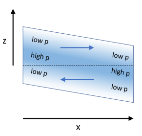
Figure 1: A cartoon of how a warp leads to horizontal pressure gradients, which lead to the “sloshing motion” of gas in the disc (blue horizontal arrows). At the inclined midplane, the gas pressure is the highest (’high p’ in the figure), while in the disc atmosphere it is lower (’low p’ in the figure). The coordinates $x$ and $z$ are the local coordinates used for the shearing box in this paper. This cartoon was inspired by the cartoon in Figure 5 of Ogilvie & Latter (2013a).

It was shown by Papaloizou & Pringle (1983) that the oscillating horizontal pressure gradients produced by the oscillating vertical offset between adjacent annuli (see Fig. 1) leads to strong horizontal epicyclic motions in the disc with an amplitude proportional to the distance $z^{\prime}$ from the disc’s midplane. These oscillations, in turn, produce an orbit-averaged torque that completely dominates any of the viscous torques. These motions are similar to the “sloshing motion” of a layer of water on a tray that undergoes an oscillating tilt. Although these are usually referred to as “resonant motions” in the literature, we will call them “sloshing motions” from here on. The key to understanding the internal torque in the disc is therefore to understand the behavior of these sloshing motions.

Papaloizou & Pringle (1983) and Papaloizou & Lin (1995) showed that for viscosities $\alpha_{t}>h_{p}/r$ (where $h_{p}$ is the pressure scale height of the disc and $\alpha_{t}$ the usual viscosity parameter) the global behavior of a disc warp is to damp out in a diffusive manner, while for lower viscosity the warp propagates as a wave. Using an asymptotic expansion method, Ogilvie (1999) and Lubow & Ogilvie (2000) derived, from first principles, self-consistent equations for these two regimes. In the diffusive regime ($\alpha_{t}>h_{p}/r$), the sloshing motion is, at all times, in a local steady state of oscillation that depends only on the local conditions and the local warp amplitude. The resulting internal torque vector ${\bf G}{}$ can therefore be computed uniquely from these local conditions. In the wave-like regime ($\alpha_{t}<h_{p}/r$), the sloshing motion never finds the time to reach a local oscillatory steady-state, because the disc geometry changes faster than this steady state can be reached. The resulting internal torque vector ${\bf G}{}$ therefore becomes a dynamic quantity. The local conditions do not determine the torque, but only determine its time derivative. As a result, a warp propagates as a wave.

Finding a set of equations that is valid in both regimes, and also self-consistently includes the radial viscous mass transport in the disk, requires an understanding of how the sloshing motions and the resulting internal torque behave when the time scale for the sloshing motion to reach a local steady-state oscillation is similar to the time scale by which the disc geometry itself changes. Martin et al. (2019) have done this empirically by starting from the time-dependent equation for the internal torque from the wavelike regime, and adding terms such that, for sufficiently large $\alpha_{t}$, the resulting asymptotic torque becomes equal to the one derived for the diffusive regime.

The aim of our paper is to derive the time-dependent equations for ${\bf G}{}$, valid in both the diffusive and the wavelike regime, from first principles, by studying the sloshing motion itself. To this end we will zoom in to a local annulus of the disc, and employ the warped shearing box framework of Ogilvie & Latter (2013a) to derive these equations. The resulting equations (Eqs. 83, 84) are those of a driven and damped harmonic oscillator. When initiated with a given initial condition, the oscillation evolves, and eventually reaches a steady-state oscillation (Eqs. 88, 89, provided the local warp does not change). The steady-state oscillation solutions were described in Ogilvie & Latter (2013a). The key to finding the link between the diffusive and wavelike regime lies in including the dynamics that can occur before this steady state solution is reached (Eqs. 90, 91). For large amplitudes of the sloshing motion the equations become non-linear, which would require a numerical treatment. For sufficiently small amplitudes, however, the linear set of equations allow the solution to be written as a steady-state particular solution plus a transient homogeneous solution (Eqs. 85, 86). The steady-state particular solution is identical to the solution described in Ogilvie & Latter (2013a). The transient homogeneous solution describes how the sloshing motion approaches this particular solution for any given initial condition. After transforming these solutions to the lab frame (Eqs. 103, 104), we derive the resulting internal torque vector components (Eqs. 127, 128).

Given that the decay of the homogeneous solution takes often much more time than the change in the disc geometry, we cannot just use this description of the sloshing motion and the resulting internal torque vector. Instead, we cast this behavior of the internal torque vector into a local ordinary differential equation (Eq. 161). This leads to the first version of the generalized warped disc equations we propose in this paper (Eq. 165, together with the equations in Section 3, valid for small warps). We will compare our equations to those in the literature in the appropriate limits (diffusion limit and wavelike limit) and find general agreement.

However, in agreement with Martin et al. (2019), we find that the full set of equations display a spurious behavior in the viscous evolution of the surface density $\Sigma(r,t)$ of the disc, even in regions of the disc where the warp wave has already passed. The cause of this behavior lies in the fact that our equations, and those in the literature, do not account for what happens when the orbital plane of the disc annulus changes its orientation (which will doubtlessly happen as a result of the torques themselves, and possibly due to an external torque as well). The corresponding correction terms to the equations cannot be readily derived from the shearing box analysis, since in that analysis the box is kept at a fixed orientation. Instead, we argue that the internal torque vector co-rotates along with any rotation of the orientation vector, because otherwise the torque vector will become unphysical. We propose a rotation-inducing correction term to our equations and demonstrate that this yields a physically correct behavior of the combined evolution of the warp and the surface density. This leads to the second and final version of our proposed generalized equation for the internal torque, valid for small warps (Eq. 172).

Martin et al. (2019) follow a different approach: they use damping terms to damp away the unphysical parts of the internal torque vector. We compare our approach to theirs and show that both approaches lead to compatible results, though our approach results in a less stiff set of equations and does not require a free tuning parameter such as the $\beta$ parameter of Martin et al. (2019).

Finally, we will show how our set of equations can be intuitively interpreted using the affine tilted slab picture of Ogilvie (2018), thereby resolving the apparent “first glance misconception” mentioned above.

3 Setting the scene: Global conservation equations

Before zooming in onto the shearing box, it is useful to recall the global conservation laws that govern the evolution of the disc. Mass conservation is given by the following partial differential equation:

$$\frac{\partial\Sigma}{\partial t}+\frac{1}{r}\frac{\partial}{\partial r}\big{(}r\Sigma v_{r}\big{)}=0$$ (1)

where $v_{r}$ is the radial velocity of the gas and $\Sigma$ is the surface density. Angular momentum conservation is a vector-valued partial differential equation. Define the angular momentum per unit surface area

$${\bf L}(r,t)\equiv\Sigma(r,t)\,\Omega(r)\,r^{2}{\bf l}{}(r,t)$$ (2)

where $\Omega(r)$ is the orbital angular frequency at radius $r$, and ${\bf l}{}(r,t)$ is the unit vector perpendicular to the disk annulus of radius $r$. The vector ${\bf l}{}(r,t)$ is a dynamic quantity describing the warp geometry and its evolution. Angular momentum conservation is now given by

$$\frac{\partial{\bf L}}{\partial t}+\frac{1}{r}\frac{\partial}{\partial r}\big{(}r{\bf L}{}v_{r}+r{\bf G}{}\big{)}={\bf T}{}$$ (3)

where ${\bf G}{}$ is the internal torque vector and ${\bf T}{}$ is a possible external torque. Although Eq. (3) is formulated in terms of ${\bf L}$, it is, actually, the equation of motion for ${\bf l}{}(r,t)$. The two conservation equations can be combined to find an expression for the radial velocity $v_{r}$ (Martin et al., 2019):

$$v_{r}=-\frac{\partial(r{\bf G})/\partial r\cdot{\bf l}}{r\Sigma\,\partial(\Omega r^{2})/\partial r}$$ (4)

The computation of the internal torque vector ${\bf G}{}$ is the subject of this paper, which we will do by studying the disk with a shearing box analysis. We will show that ${\bf G}{}$ is governed by Eqs. (153, 156, 173). Some readers may be more familiar with another form of the warped disk equations. We will discuss the relation between these two forms in Appendix A.

4 Local warped shearing box equations

4.1 Basics

Ogilvie & Latter (2013a) presented the “warped shearing box” approach for studying the local internal dynamics of the gas in a warped disc. We will largely follow their path, with only minor modifications of notation. We refer to that paper for an introduction to the concepts of this approach.

In classical viscous disc theory, the disc is described as a continuous set of concentric annuli as a function of radius $r$. The mass distribution is described by the surface density $\Sigma(r)$, and viscous disc theory describes how this function changes with time: $\Sigma(r,t)$. In a warped disc, also the inclination is dependent on radial coordinate. Let ${\bf l}{}(r)$ be the unit vector perpendicular to the disc annulus at radius $r$, then a non-zero $d{\bf l}{}/dr$ is what is called a warp. Let us define the warp vector as

$${\boldsymbol{\psi}}(r)=\frac{d{\bf l}(r)}{d\ln r}$$ (5)

and the warp amplitude Ogilvie (1999) as

$$\psi(r)=\left|{\boldsymbol{\psi}}(r)\right|$$ (6)

The viscous evolution of a warped disc describes the time-dependence of $\Sigma(r,t)$ and ${\bf l}{}(r,t)$ for a given initial condition. Since this evolution is driven by the conservation and transport of angular momentum through the disc (see Section 3), we need to derive equations for the internal torque ${\bf G}{}(r,t)$. This is where the shearing box model comes in. To apply the shearing box framework to a warped disc we choose a radius $r_{0}$ and define the global laboratory frame $(X,Y,Z)$ coordinate system such that ${\bf l}{}(r_{0})$ points in the $Z$-direction, and that the warp vector $d{\bf l}{}/d\ln r$ points into positive $X$ direction (see Fig. 2). Note that Fig. 1 of Ogilvie & Latter (2013a) gives a 3-D illustration of this geometry, where their ${\bf m}$ vector is the unit vector in $X$-direction, ${\bf e}_{X}$, and their ${\bf n}$ vector is the unit vector in $Y$-direction, ${\bf e}_{Y}$. Along the circular orbit at $r=r_{0}$ we define the azumuthal coordinate $\phi$ counter-clockwise, with $\phi=0$ at the positive $X-$axis, i.e. $X(r=r_{0},\phi)=r_{0}\cos(\phi)$ and $Y(r=r_{0},\phi)=r_{0}\sin(\phi)$. The gas rotates in the direction of increasing $\phi$ with an orbital angular frequency $\Omega_{0}=\Omega(r=r_{0})$. As Ogilvie & Latter (2013a) we define $q$ as

$$q=-\frac{d\ln\Omega}{d\ln r}$$ (7)

which, for perfectly Keplerian orbits, is $q=3/2$. However, in realistic discs, $q$ can deviate slightly from $3/2$. In protoplanetary discs this is due to the radial pressure gradient, or external influences, such as a binary companion (e.g. Zanazzi & Lai, 2018b), or magnetic torques (e.g. Lai, 1999, 2003).

4.2 Unwarped shearing box coordinates

In the classical shearing box framework we follow the orbital motion of the gas near radius $r_{0}$ and define local coordinates $(x,y,z)$ such that the origin comoves along the orbit at $r=r_{0}$ at orbital angular frequency $\Omega_{0}=\Omega(r=r_{0})$, and rotates such that $x$ always points outwards, $y$ always stays tangent to the orbit, and $z$ always points upward (parallel to ${\bf l}{}(r=r_{0})$). The velocity components $(u_{x},u_{y},u_{z})$ are defined as the comoving time derivatives of the location of a test particle or fluid parcel in this local coordinate system: $u_{x}=D_{t}x(t)$, $u_{y}=D_{t}y(t)$, $u_{z}=D_{t}z(t)$.

In this local coordinate system the equations of motion of a test particle or a fluid parcel are:

$$D_{t}x = u_{x}$$ (8)

$$D_{t}y = u_{y}$$ (9)

$$D_{t}z = u_{z}$$ (10)

$$D_{t}u_{x}-2\Omega_{0}u_{y} = f_{x}+2q\Omega_{0}^{2}x$$ (11)

$$D_{t}u_{y}+2\Omega_{0}u_{x} = f_{y}$$ (12)

$$D_{t}u_{z} = f_{z}-\Omega_{0}^{2}z$$ (13)

where $f_{i}$ (with $i=x,y,z$) are the forces per unit mass acting on the test particle or fluid parcel. In case of a fluid parcel, these forces include the pressure gradient force and the viscous forces, which we will discuss later, plus external forces, if present. The $2q\Omega_{0}^{2}x$ term in Eq. (11) is the sum of the outward-pointing centrifugal force and the inward-pointing gravitational force, which, at $x=0$, are in perfect balance. The second terms on the left-hand-side of Eqs. (11, 12) are the Coriolis forces. The $-\Omega_{0}^{2}z$ term in Eq. (13) is the vertical component of the gravitational force.

In the simple case of zero viscosity and no external forcing, only the gradient of the gas pressure $p$ enters in the $f_{i}$ terms (let us call these $f^{p}_{i}$):

$$f_{x}^{p}=\rho^{-1}\partial_{x}p,\qquad f_{y}^{p}=\rho^{-1}\partial_{y}p,\qquad f_{z}^{p}=\rho^{-1}\partial_{z}p$$ (14)

where $\rho$ is the gas density. For a non-warped laminar disc one can set $\partial_{y}p=0$ and $\partial_{x}p=0$ (a global radial pressure gradient cannot be consistently included in a local shearing box model, except as a pseudo-force). A simple solution is then $u_{x}=0$, $u_{y}=-q\Omega_{0}x$ and $u_{z}=0$. What remains is to solve for the vertical density structure from Eq. (13):

$$\frac{1}{\rho(z)}\frac{\partial p(z)}{\partial z}=-\Omega_{0}^{2}z$$ (15)

For the simple isothermal case we set $p=\rho c_{s}^{2}$ with the isothermal sound speed $c_{s}$ set to a constant. The solution is then

$$\rho(z)=\frac{\Sigma}{\sqrt{2\pi}h_{p}}\exp\left(-\frac{z^{2}}{2h_{p}^{2}}\right)$$ (16)

with $\Sigma$ the surface density, and $h_{p}=c_{s}/\Omega_{0}$ the pressure scale height.

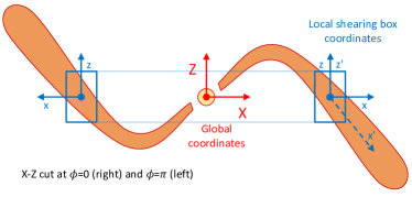
Figure 2: A cartoon of the geometry of the warped disk and coordinate systems used, shown as a vertical cut through the disk. Here only the $\phi=0$, $\phi=\pi$ (i.e. the $X-Z$) plane is shown. The global coordinates $(X,Y,Z)$ are, for the derivation of the equations, chosen such that $d{\bf l}/d\ln r$ points in $X$-direction.

4.3 Warped shearing box coordinates

For a warped disk the geometry is pictographically shown in Fig. 2, where the amplitude of the warp has been exaggerated for clarity. The warped version of the shearing box framework of Ogilvie & Latter (2013a) introduces “warped local coordinates” $(x^{\prime},y^{\prime},z^{\prime})$ which adjust themselves to the warped geometry:

$$x = x^{\prime}$$ (17)

$$y = y^{\prime}$$ (18)

$$z = z^{\prime}-\psi x^{\prime}\cos(\phi)$$ (19)

The $z^{\prime}$ coordinate thus follows the up-and-down oscillation of the gas at $x^{\prime}\neq 0$ as a result of the disc warp. The $(x^{\prime},z^{\prime})$ coordinate geometry is shown in Fig. 2 on the right side of the figure. It is also nicely visualized in the right panel of figure 4 of Ogilvie & Latter (2013a). However, as one can see from Eq. (18), in constrast to Ogilvie & Latter (2013a), we do not modify $y^{\prime}$ to follow the azimuthal shearing motion of the gas in the disc because it would lead to an incessant “winding up” of the $y^{\prime}$ coordinate. Therefore, the left panel of figure 4 of Ogilvie & Latter (2013a) does not apply to our $(x^{\prime},y^{\prime})$ geometry.

The new vertical coordinate $z^{\prime}$ is the vertical coordinate with respect to the midplane of the warped disc. Therefore, in first approximation, the vertical density structure for the warped disc can thus be described by Eq. (16) with $z$ replaced by $z^{\prime}$.

As the fluid parcel orbits around the star, the azimuth will change according to $\phi=\Omega_{0}t$, where the zero time $t=0$ is chosen to be when the parcel was at $\phi=0$.

In the warped shearing box coordinates one can define the velocity components in a similar way as in the unwarped case: $u_{x}^{\prime}=D_{t}x^{\prime}(t)$, $u_{y}^{\prime}=D_{t}y^{\prime}(t)$, $u_{z}^{\prime}=D_{t}z^{\prime}(t)$. However, it is useful to define new velocities $(v_{x}^{\prime},v_{y}^{\prime},v_{z}^{\prime})$ such that

$$u_{x}^{\prime}=v_{x}^{\prime},\quad u_{y}^{\prime}=v_{y}^{\prime}-q\Omega_{0}x^{\prime},\quad u_{z}^{\prime}=v_{z}^{\prime}+\psi\cos(\phi)v_{x}^{\prime}$$ (20)

with $\phi=\Omega_{0}t$ for the fluid parcel we follow. In relation to the unwarped coordinate velocities we then have:

$$u_{x} = v_{x}^{\prime}$$ (21)

$$u_{y} = v_{y}^{\prime}-q\Omega_{0}x^{\prime}$$ (22)

$$u_{z} = v_{z}^{\prime}+\psi\Omega_{0}x^{\prime}\sin(\phi)$$ (23)

where we used Eq. (201) of Appendix B.1. The advantage of the velocities $(v_{x}^{\prime},v_{y}^{\prime},v_{z}^{\prime})$ compared to $(u_{x}^{\prime},u_{y}^{\prime},u_{z}^{\prime})$ is that they are orthogonal velocities, in spite of the skewed coordinate system $(x^{\prime},y^{\prime},z^{\prime})$. We call this a “half-mixed frame” because it is mixed-frame in $y$-direction but fully comoving frame in $z$-direction (and in $x$-direction it remains fixed to the shearing box).

In terms of these “half-mixed frame” warped coordinates and velocities, the equations of motion of a test particle or a fluid parcel are (see Appendix B.1):

$$D_{t}x^{\prime} = v_{x}^{\prime}$$ (24)

$$D_{t}y^{\prime} = v_{y}^{\prime}-q\Omega_{0}x^{\prime}$$ (25)

$$D_{t}z^{\prime} = v_{z}^{\prime}+\psi v_{x}^{\prime}\cos(\phi)$$ (26)

$$D_{t}v_{x}^{\prime}-2\Omega_{0}v_{y}^{\prime} = f_{x}$$ (27)

$$D_{t}v_{y}^{\prime}+(2-q)\Omega_{0}v_{x}^{\prime} = f_{y}$$ (28)

$$D_{t}v_{z}^{\prime}+\psi\Omega_{0}\sin(\phi)v_{x}^{\prime} = f_{z}-\Omega_{0}^{2}z^{\prime}$$ (29)

For the fluid dynamics we also need the continuity equation:

$$D_{t}\rho=-\rho\nabla\cdot{\bf u}$$ (30)

which can, with the help of Eq. (210), be written in warped coordinates as:

$$D_{t}\ln\rho=-(\partial_{x^{\prime}}+\psi\cos(\phi)\partial_{z^{\prime}})v_{x}^{\prime}-\partial_{y^{\prime}}v_{y}^{\prime}-\partial_{z^{\prime}}v_{z}^{\prime}$$ (31)

Next we turn to the forces $f_{i}$ (with $i=x,y,z$), which consist of the pressure gradient force $f_{i}^{p}$, the shear viscosity force $f_{i}^{v}$, and possibly an external force $f_{i}^{e}$:

$$f_{i}=f_{i}^{p}+f_{i}^{v}+f_{i}^{e}$$ (32)

The pressure gradient force components in warped coordinates become (see Eq. 207):

$$f_{x}^{p} = -(1/\rho)(\partial_{x^{\prime}}+\psi\cos(\phi)\partial_{z^{\prime}})p$$ (33)

$$f_{y}^{p} = -(1/\rho)\partial_{y^{\prime}}p$$ (34)

$$f_{z}^{p} = -(1/\rho)\partial_{z^{\prime}}p$$ (35)

The expressions for the shear viscosity forces $f^{v}_{i}$ in warped coordinates are complex and their derivation cumbersome, so we defer this to Appendix B.2.

The equations of this section are the fluid equations in Lagrange form. The comoving time derivative $D_{t}$ in all the above equations can be written as $\partial_{t^{\prime}}$ plus partial derivatives in $x^{\prime}$, $y^{\prime}$ and $z^{\prime}$ using Eq. (211), yielding the equations in the comoving laboratory frame (defined as the $x^{\prime}$, $y^{\prime}$ and $z^{\prime}$ warped coordinate system). This forms a set of coupled partial differential equations for the motion of the fluid (gas) in the warped shearing box.

4.4 Dimensionless time

For the following analysis it will be convenient to scale all the equations to a dimensionless time defined by

$$\tau=\Omega_{0}t$$ (36)

It is no coincidence that for a particle or fluid parcel $\tau=\phi$, as the dimensionless time corresponds to the location along the orbit. In the following we will use $\tau$ when we follow the fluid parcel along its orbit, and $\phi$ when we put emphasis on the geometric location along the orbit. We can then write

$$D_{t}=\Omega_{0}D_{\tau}$$ (37)

Equations (31, 27, 28, 29) then become:

$$\Omega_{0}D_{\tau}\ln\rho = -(\partial_{x^{\prime}}+\psi\cos(\phi)\partial_{z^{\prime}})v_{x}^{\prime}$$ (38)

$$-\partial_{y^{\prime}}v_{y}^{\prime}-\partial_{z^{\prime}}v_{z}^{\prime}$$

$$D_{\tau}v_{x}^{\prime}-2v_{y}^{\prime} = \Omega_{0}^{-1}f_{x}$$ (39)

$$D_{\tau}v_{y}^{\prime}+(2-q)v_{x}^{\prime} = \Omega_{0}^{-1}f_{y}$$ (40)

$$D_{\tau}v_{z}^{\prime}+\psi\sin(\phi)v_{x}^{\prime} = \Omega_{0}^{-1}f_{z}-\Omega_{0}z^{\prime}$$ (41)

4.5 Equations for laminar solutions

Although the equations derived so far are valid for general flows in the warped shearing box framework, in the remainder of this paper we are concerned with laminar solutions that are locally translationally symmetric in $x^{\prime}$ and $y^{\prime}$. This allows an analytic treatment. It should, however, be kept in mind that in making this assumption (and in fact, by using the shearing box approach in the first place) we are rejecting potentially important physics, which may affect the outcome (see further discussion in Section 8.3).

The assumption of translational symmetry in $x^{\prime}$ and $y^{\prime}$ has the simplifying consequence that $\partial_{x^{\prime}}=0$ and $\partial_{y^{\prime}}=0$. Furthermore we can safely set $x^{\prime}=0$ and $y^{\prime}=0$. This already removes a number of terms in the equations.

Next we make the simplifying assumption of a vertically isothermal equation of state, as we did at the end of Subsection 4.2. The vertical density structure is then identical to the Gaussian solution of Eq. (16), but with $z$ replaced by $z^{\prime}$:

$$\rho(z^{\prime},\tau)=\frac{\Sigma}{\sqrt{2\pi}h_{p}(\tau)}\exp\left(-\frac{(z^{\prime})^{2}}{2h_{p}(\tau)^{2}}\right)$$ (42)

In fact, if we make the additional assumption that all velocities $v_{x}^{\prime}$, $v_{y}^{\prime}$ and $v_{z}^{\prime}$ are zero at $z^{\prime}=0$ and linearly proportional to $z^{\prime}$, then the Gaussian structure of Eq. (42) remains valid even while $\partial_{z^{\prime}}v_{z}^{\prime}\neq 0$, i.e. during vertical compression or expansion. The time-dependence of the entire vertical density profile can then be described by the time-dependence of a single parameter: the pressure scale height $h_{p}(\tau)$.

Following Ogilvie & Latter (2013a) we therefore look for solutions to the velocity variables of the form:

$$v_{x}^{\prime}(z^{\prime},\tau) = V_{x}(\tau)\Omega_{0}z^{\prime}$$ (43)

$$v_{y}^{\prime}(z^{\prime},\tau) = V_{y}(\tau)\Omega_{0}z^{\prime}$$ (44)

$$v_{z}^{\prime}(z^{\prime},\tau) = V_{z}(\tau)\Omega_{0}z^{\prime}$$ (45)

Inserting these into Eqs. (38-41) yields:

$$D_{\tau}\ln\rho = -\psi\cos(\phi)V_{x}-V_{z}$$ (46)

$$\bar{D}_{\tau}V_{x}-2V_{y} = (\Omega_{0}^{2}z^{\prime})^{-1}f_{x}$$ (47)

$$\bar{D}_{\tau}V_{y}+(2-q)V_{x} = (\Omega_{0}^{2}z^{\prime})^{-1}f_{y}$$ (48)

$$\bar{D}_{\tau}V_{z}+\psi\sin(\phi)V_{x} = (\Omega_{0}^{2}z^{\prime})^{-1}f_{z}-1$$ (49)

where $\bar{D}_{\tau}V_{i}$ (with $i=x,y,z$) is defined as

$$\begin{split}\bar{D}_{\tau}V_{i}&\equiv D_{\tau}V_{i}+V_{i}\frac{1}{z^{\prime}}D_{\tau}z^{\prime}\\ &=\partial_{\tau}V_{i}+V_{i}\big{(}V_{z}+\psi\cos(\phi)V_{x}\big{)}\end{split}$$ (50)

where in the second term we used Eqs. (37, 211).

Clearly only forces are allowed that vanish at $z^{\prime}=0$, for otherwise these equations become singular. In fact, for solutions to exist, the $f_{i}$ forces also have to be linear in $z^{\prime}$. Indeed, this happens to be true automatically for the pressure gradient force $f^{p}_{i}$ and the shear viscosity force $f^{v}_{i}$, if one applies the Gaussian vertical structure of Eq. (42). For the pressure gradient force $f^{p}_{i}$ we start with Eqs. (33-35) and set $\partial_{x^{\prime}}=0$ and $\partial_{y^{\prime}}=0$ to obtain:

$$f_{x}^{p} = -(1/\rho)\psi\cos(\phi)\partial_{z^{\prime}}p$$ (51)

$$f_{y}^{p} = 0$$ (52)

$$f_{z}^{p} = -(1/\rho)\partial_{z^{\prime}}p$$ (53)

Now use Eq. (42) for computing the $\partial_{z^{\prime}}p$ by setting $p=\rho c_{s}^{2}$ and keeping $c_{s}^{2}$ constant. This yields

$$\partial_{z^{\prime}}p=c_{s}^{2}\partial_{z^{\prime}}\rho=-\rho c_{s}^{2}\frac{z^{\prime}}{h_{p}^{2}}$$ (54)

where $h_{p}(\tau)$ can be time-dependent. From the non-warped disc geometry we know that the equilibrium value of $h_{p}$ is $c_{s}/\Omega_{0}$ (see Section 4.2). So let us define the dimensionless pressure scale height $H$ as

$$h_{p}(\tau)=H(\tau)\frac{c_{s}}{\Omega_{0}}$$ (55)

This then leads to

$$\frac{1}{\rho}\partial_{z^{\prime}}p=-\frac{\Omega_{0}^{2}}{H^{2}}\;z^{\prime}$$ (56)

which leads to the following expressions for the pressure gradient forces

$$(\Omega_{0}^{2}z^{\prime})^{-1}f_{x}^{p} = \psi\cos(\phi)H^{-2}$$ (57)

$$(\Omega_{0}^{2}z^{\prime})^{-1}f_{y}^{p} = 0$$ (58)

$$(\Omega_{0}^{2}z^{\prime})^{-1}f_{z}^{p} = H^{-2}$$ (59)

Before we devote our attention to the viscosity forces, let us rewrite the $D_{\tau}\ln\rho$ term in Eq. (46). Using again the Gaussian vertical density structure of Eq. (42) and realizing that in the comoving derivative the $(z^{\prime})^{2}/h_{p}(\tau)^{2}$ inside the exponent stays constant (the vertical structure shrinks or expands vertically in a self-similar way), we find

$$D_{\tau}\ln\rho=-D_{\tau}\ln H=-\partial_{\tau}\ln H$$ (60)

This allows us to write the equations for $V_{x}(\tau)$, $V_{y}(\tau)$, $V_{z}(\tau)$ and $H(\tau)$ (Eqs. 46-49) as

$$\partial_{\tau}\ln H = \psi\cos(\phi)V_{x}+V_{z}$$ (61)

$$\bar{D}_{\tau}V_{x}-2V_{y} = \psi\cos(\phi)H^{-2}+F^{\mathrm{ve}}_{x}$$ (62)

$$\bar{D}_{\tau}V_{y}+(2-q)V_{x} = F^{\mathrm{ve}}_{y}$$ (63)

$$\bar{D}_{\tau}V_{z}+\psi\sin(\phi)V_{x} = H^{-2}-1+F^{\mathrm{ve}}_{z}$$ (64)

where $F^{\mathrm{ve}}_{i}$ are the viscous and external forces in the form:

$$F^{\mathrm{ve}}_{i}\equiv F^{\mathrm{v}}_{i}+F^{\mathrm{e}}_{i}\equiv(\Omega_{0}^{2}z^{\prime})^{-1}(f^{v}_{i}+f^{e}_{i})$$ (65)

Bulk viscosity can be included as a hysteresis factor in the pressure, dependent on $\nabla\cdot{\bf u}$, but we will not include this in this analysis.

Note, incidently, that the right-hand-side of Eq. (61) happens to be the same as the term in brackets in Eq. (50). And so one can write Eq. (50) as

$$\bar{D}_{\tau}V_{i}=\partial_{\tau}V_{i}+V_{i}\,\partial_{\tau}\ln H$$ (66)

Together with the expressions for the viscous forces $F^{\mathrm{v}}_{i}$ from appendix B.2 (Eqs. 246-248), and any possible external $F^{\mathrm{v}}_{e}$, the set of equations Eqs. (61-64) with $\phi=\tau$ is complete, and can be integrated in time $\tau$ for any initial condition of $H$, $V_{x}$, $V_{y}$ and $V_{z}$. A recommended way to integrate these is by using a numerical integrator such as the solve_ivp() method from the scipy.integrate library of Python, which is a higher-order integration scheme that automatically adjusts step size to control the error, and is easy to use (Virtanen et al., 2020).

5 Solutions for the sloshing motion

5.1 Vertical and horizontal oscillations

As pointed out by Ogilvie & Latter (2013a), for the non-warped case ($\psi=0$), and for zero viscosity, the equation set Eqs. (61-64) has two oscillating modes: A vertical oscillation (called the “breathing mode” by Ogilvie & Latter (2013a)) coupling Eqs. (61 and 64), and a horizontal epicyclic oscillation mode (which we call the “sloshing motion”) coupling Eqs. (62 and 63).

This can be seen a bit clearer if we linearize Eqs. (61-64). Let us define an alternative variable to $H$:

$$H=e^{W}{}=1+W{}+{\cal O}(W{}^{2})$$ (67)

and assume $|W{}|\ll 1$. Now we remove all terms that are of second or higher order in $(W{},V_{x},V_{y},V_{z})$. We arrive at:

$$\partial_{\tau}W{} = \psi\cos(\phi)V_{x}+V_{z}$$ (68)

$$\partial_{\tau}V_{x}-2V_{y} = \psi\cos(\phi)(1-2W{})+F^{\mathrm{ve}}_{x}$$ (69)

$$\partial_{\tau}V_{y}+(2-q)V_{x} = F^{\mathrm{ve}}_{y}$$ (70)

$$\partial_{\tau}V_{z}+\psi\sin(\phi)V_{x} = -2W{}+F^{\mathrm{ve}}_{z}$$ (71)

For $\psi=0$ and $F^{\mathrm{ve}}_{i}=0$, the two modes decouple. The breathing mode has a frequency $\Omega_{b}=\sqrt{2}\Omega_{0}$, while the sloshing mode oscillates at the epicyclic frequency

$$\Omega_{e}=\sqrt{2(2-q)}\,\Omega_{0}$$ (72)

It will be convenient for the remainder of this paper to define these (and other) frequencies in units of the dimensionless time $\tau$. From here onward we define the dimensionless breathing mode frequency $\omega_{b}=\Omega_{b}/\Omega_{0}=\sqrt{2}$, and the dimensionless epicyclic frequency $\kappa$ as

$$\kappa=\Omega_{e}/\Omega_{0}=\sqrt{2(2-q)}$$ (73)

For an exactly keplerian disc, $q=3/2$, and therefore $\kappa=1$.

If no bulk viscosity is included, the breathing mode remains undamped. In practice it is likely that such modes will propagate as waves through the disc in radial direction, but that cannot be described within the framework used here. If no shear viscosity is included, the epicylic oscillation will also be undamped. Also in this case it may be that the epicyclic oscillations of neighboring annuli interact, but, again, this is outside of the scope of the present framework.

For a warped disc, $\psi\neq 0$, the two modes couple, albeit only weakly if $\psi\ll 1$.

5.2 Solutions to the linearized equations

The linearized equations Eqs. (68-71) allow simple analytic solutions if all terms proportional to the product of $\psi$ with one of the variables $(W{},V_{x},V_{y},V_{z})$ are considered small and are ignored. The equations then reduce to:

$$\partial_{\tau}W{} = V_{z}$$ (74)

$$\partial_{\tau}V_{x}-2V_{y} = \psi\cos(\phi)+F^{\mathrm{ve}}_{x}$$ (75)

$$\partial_{\tau}V_{y}+(2-q)V_{x} = F^{\mathrm{ve}}_{y}$$ (76)

$$\partial_{\tau}V_{z} = -2W{}+F^{\mathrm{ve}}_{z}$$ (77)

The viscous forces (Eqs. 246-248) then reduce to:

$$F_{x}^{v} = -\alpha_{t}\big{(}V_{x}+\psi\sin(\phi)\big{)}$$ (78)

$$F_{y}^{v} = -\alpha_{t}\big{(}V_{y}-q\psi\cos(\phi)\big{)}$$ (79)

$$F_{z}^{v} = -\alpha_{t}\big{(}\tfrac{4}{3}V_{z}+\psi^{2}\sin(\phi)\cos(\phi)\big{)}$$ (80)

The removal of these $\psi W{}$ and $\psi V_{i}$ terms has the consequence that the vertical and horizontal oscillations decouple completely. Of relevance to the internal torque is only the oscillation in $V_{x}$ and $V_{y}$: the sloshing motion. Let us set the external force $F^{e}_{i}=0$, and insert $F^{v}_{x}$ and $F^{v}_{y}$ into Eqs. (75,76):

$$\partial_{\tau}V_{x}-2V_{y}\kern-5.0pt = \kern-5.0pt\psi(\cos(\phi)-\alpha_{t}\sin(\phi))-\alpha_{t}V_{x}$$ (81)

$$\partial_{\tau}V_{y}+(2-q)V_{x}\kern-5.0pt = \kern-5.0pt\alpha_{t}q\psi\cos(\phi)-\alpha_{t}V_{y}$$ (82)

where, again, we use $\phi=\tau$. And so, after a long journey, we have arrived at two coupled linear ordinary differential equations for the sloshing motion that can be solved analytically for $V_{x}(\tau)$ and $V_{y}(\tau)$.

For this analytical treatment it is convenient to replace $\cos(\phi)$ with $e^{i\phi}$ and $\sin(\phi)$ with $-ie^{i\phi}$, solve for the complex versions of $V_{x}(\tau)$ and $V_{y}(\tau)$, and then take the real part of these. Eqs. (81,82) become:

$$\partial_{\tau}V_{x}-2V_{y}\kern-5.0pt = \kern-5.0pt\psi(1+i\alpha_{t})e^{i\phi}-\alpha_{t}V_{x}$$ (83)

$$\partial_{\tau}V_{y}+(2-q)V_{x}\kern-5.0pt = \kern-5.0pt\alpha_{t}q\psi e^{i\phi}-\alpha_{t}V_{y}$$ (84)

We now seek solutions of the form

$$V_{x}(\tau) = V_{xp}(\tau)+V_{xh}(\tau)$$ (85)

$$V_{y}(\tau) = V_{yp}(\tau)+V_{yh}(\tau)$$ (86)

where $V_{ip}(\tau)$ are the harmonic particular solution and $V_{ih}(\tau)$ are the homogeneous solution. The particular solution can be written as

$$V_{xp}(\tau)=V_{xp0}e^{i\tau},\qquad V_{yp}(\tau)=V_{yp0}e^{i\tau}$$ (87)

with

$$V_{xp0} = \frac{\alpha_{t}(4-\kappa^{2})+i(1+\alpha_{t}^{2})}{\kappa^{2}+(i+\alpha_{t})^{2}}\;\psi$$ (88)

$$V_{yp0} = \frac{2\alpha_{t}(i+\alpha_{t})-\tfrac{1}{2}\kappa^{2}(\alpha_{t}^{2}+2i\alpha_{t}+1)}{\kappa^{2}+(i+\alpha_{t})^{2}}\;\psi$$ (89)

where $\kappa=\sqrt{2(2-q)}$. The homogeneous solution can be written as

$$V_{xh}(\tau)=V_{xh0}e^{i\omega\tau},\qquad V_{yh}(\tau)=V_{yh0}e^{i\omega\tau}$$ (90)

with

$$\omega=\kappa+i\alpha_{t}$$ (91)

The values of $V_{xh0}$ and $V_{yh0}$ are related to the initial conditions $V_{x}(\tau=0)$ and $V_{y}(\tau=0)$ through

$$V_{ih0}=V_{i}(\tau=0)-V_{ip0}$$ (92)

With this, we now have the complete family of solutions for the sloshing oscillation in the linear regime for sufficiently small $\psi$ that the $\psi W{}$ and $\psi V_{i}$ terms can be neglected. For non-small $\psi$, the inclusion of these terms still keeps the problem linear in $(W{},V_{x},V_{y},V_{z})$, but the solution will acquire higher-order modes, and the problem will become substantially more difficult. In that case, as well as in the case that the linear approximation becomes invalid, a numerical treatment is preferable.

5.3 The $(\tau,\phi)$ picture and the real time-dependence

So far we have looked at a parcel of gas in the azimuthal comoving frame, where $\tau$ can be regarded as equivalent to azimuth $\phi$. However, if the solution at $\tau=2\pi$ is not the same as the starting point at $\tau=0$, then this equivalence of $\tau$ and $\phi$ is invalid. Furthermore, while we see time-dependent behavior when moving along with a fluid parcel as it orbits around the star, the behavior of the entire annulus, seen in the lab frame, may be stationary or only slowly varying in time.

It is therefore better to look at the dynamics as a function of time $\tau$ and azimuthal angle $\phi$, i.e. $V_{x}(\tau,\phi)$ and likewise for the other quantities. We will now assume that the $\phi$-dependence is $e^{im\phi}$ at all times, and choose $m=1$, because a warp is by definition an $m=1$ mode. So we have

$$V_{x}(\tau,\phi)=V_{x}(\tau)e^{i\phi}$$ (93)

and likewise for the other quantities. This assumption is valid for the linearized equations in which all terms proportional to $\psi W{}$ and $\psi V_{i}$ are neglected (i.e. Eqs. 74-77). And since in this case the vertical “breathing” and horizontal “sloshing” motions decouple, we will from here on focus only on the “sloshing” motion, the solution of which was presented in Section 5.2.

In the $(\tau,\phi)$-picture, $V_{x}(\tau)$ is a property of the entire $2\pi$ circumference of the annulus instead of a single fluid parcel. By definition $V_{x}(\tau)$ is the value of $V_{x}(\tau,\phi)$ at dimensionless time $\tau$ and azimuth $\phi=0$. The value at any other azimuth is then a rotation $e^{i\phi}$ in the complex plane of this value. If in the previous comoving picture the mode under consideration had angular frequency $\omega=1$ (i.e. in dimensional units: angular frequency $\Omega_{0}$), then in the present $m=1$ mode picture $V_{x}(\tau)$ does not vary with $\tau$. If, on the other hand, in the previous comoving picture the mode under consideration had angular frequency $\omega\neq 1$, then in the $m=1$ mode picture, $V_{x}(\tau)$ varies with time as $V_{x}(\tau)\propto e^{i(\omega-1)\tau}$.

The comoving time derivative $D_{\tau}$ of the comoving picture now gets replaced by

$$D_{\tau}\rightarrow\partial_{\tau}+\partial_{\phi}=\partial_{\tau}+i$$ (94)

The $i$ arises due to $\partial_{\phi}e^{i\phi}=ie^{i\phi}$. The $\partial_{\tau}$ now stands for the non-comoving (lab frame) time derivative at $\phi=0$.

The new form of the dynamic equations for $V_{x}$ and $V_{y}$ (Eqs. 83, 84) now becomes:

$$\partial_{\tau}V_{x}-2V_{y} = \psi(1+i\alpha_{t})-(i+\alpha_{t})V_{x}$$ (95)

$$\partial_{\tau}V_{y}+(2-q)V_{x} = \alpha_{t}q\psi-(i+\alpha_{t})V_{y}$$ (96)

We look for solutions of the form:

$$V_{x}(\tau) = V_{xp0}+V_{xh0}e^{i\omega_{0}\tau}$$ (97)

$$V_{y}(\tau) = V_{yp0}+V_{yh0}e^{i\omega_{0}\tau}$$ (98)

where the first terms are the particular solution given by Eqs. (88, 89), and the second terms are the homogeneous solution, where $\omega_{0}=\omega-1$ is the lab-frame frequency of the homogeneous solution, where $\omega$ is given by Eq. (91), hence

$$\omega_{0}=\kappa-1+i\alpha_{t}$$ (99)

What this says is that for slightly non-Keplerian discs ($0<|\kappa-1|\ll 1$) the homogeneous part of the sloshing motion of $V_{x}(\tau,\phi)$ slowly phase-shifts in time, and at the same time (for $\alpha_{t}>0$) decays, leaving eventually only the steady-state sloshing motion $V_{xp0}e^{i\phi}$, which does not phase-shift in time. The slow phase-shift of the homogeneous solution is simply the apsidal precession of the epicyclic motion for $\kappa\neq 1$.

Note that the $V_{xp0}$ and $V_{yp0}$ are nearly perpendicular in the complex plane ($V_{yp0}$ being a phase shift $\sim\pi/2$ ahead of $V_{xp0}$), but not exactly.

For the homogeneous solution we can choose $V_{xh0}$ (a complex number) at will: it determines the initial condition of the homogeneous solution. For a chosen $V_{xh0}$, the $V_{yh0}$ follows as:

$$V_{yh0}=\frac{1}{2}i\kappa V_{xh0}$$ (100)

So, for the homogeneous solution, $V_{yh}(\tau)$ has exactly a phase shift $\pi/2$ ahead of $V_{xh}(\tau)$.

If we wish to express the initial conditions explicitly, we can write the solutions as:

$$V_{x}(\tau) = V_{xp0}+(V_{x0}-V_{xp0})e^{i\omega_{0}\tau}$$ (101)

$$V_{y}(\tau) = V_{yp0}+(V_{y0}-V_{yp0})e^{i\omega_{0}\tau}$$ (102)

where $V_{x0}=V_{x}(\tau=0)$ and $V_{y0}=V_{y}(\tau=0)$ are the initial conditions. In other words: $V_{ih0}=V_{i0}-V_{ip0}$. Clearly, for $\alpha_{t}>0$ the solution converges to the steady-state particular solution on a dimensionless time scale $1/\alpha_{t}$. And for $\kappa\neq 1$ the solution also rotates (in the complex plane) around the steady-state particular solution on a time scale $1/|\kappa-1|$.

For completeness, let us write the full solution of the shoshing motion, including the $\phi$-dependence, as well:

$$V_{x}(\tau,\phi) = V_{xp0}e^{i\phi}+(V_{x0}-V_{xp0})e^{i\omega_{0}\tau+i\phi}$$ (103)

$$V_{y}(\tau,\phi) = V_{yp0}e^{i\phi}+(V_{y0}-V_{yp0})e^{i\omega_{0}\tau+i\phi}$$ (104)

This gives, in the linear regime for sufficiently small $\psi$, a complete description of the sloshing motion in an annulus of the disc. It is time-dependent as long as the steady-state particular solution is not reached. But this time-dependence vanishes as the solution approaches the steady-state particular solution, in which case only the $m=1$ dependence on azimuth $\phi$ remains:

$$V_{x}(\tau\rightarrow\infty,\phi) = V_{xp0}e^{i\phi}$$ (105)

$$V_{y}(\tau\rightarrow\infty,\phi) = V_{yp0}e^{i\phi}$$ (106)

Note that this assumes that $\psi$ stays constant, or more precisely: that $\psi$ changes slower than the convergence of the solution to the steady-state particular solution.

Fig. 3 is a geometric representation of the sloshing motion, seen in an $(x,z)$-cut through the local disc. The sloshing motion is shown by the red velocity arrows. The skewed box shows the effect this motion has on a rectangular slab of disc material. The original slab is shown with dotted lines and it is, in actuality, an annulus of disc material. This figure shows, for four different pairs of $(\alpha_{t},\kappa-1)$, the skewing of the slab as a function of the azimuth $\phi$ along the annulus. Two things are particularly noteworthy of the results shown in this figure: Firstly, it shows that for $\kappa-1=0$ the amplitude of the sloshing, and the resulting degree of skewing of the box, becomes very large for $\alpha_{t}$ lower than $10^{-1}$. This is the result of the resonance between the orbital and epicyclic frequencies (though note that these high amplitudes may not be reached before $\psi$ changes). For the two $|\kappa-1|=0.1$ models (bottom two panels) this divergence does not occur. Secondly, the skewing in the bottom three panels are strongly phase-shifted with respect to each other. This plays a fundamental role in the nature of the internal torque arising from this sloshing motion, which is the topic of Section 6.

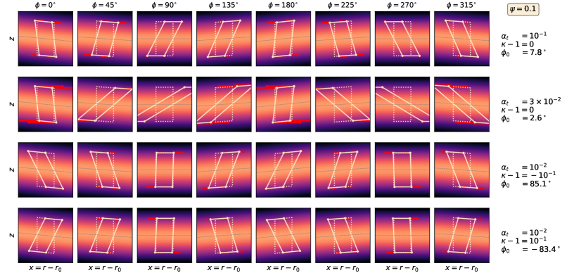
Figure 3: The local $(x,z)$ geometry of the sloshing motion of the steady-state particular solution Eq. (105) for a warp amplitude of $\psi=0.1$. The panels are arranged horizontally according to azimuth $\phi$ along the annulus of the disc, and vertically according to four pairs of model parameters $(\alpha_{t},\kappa-1)$. In each of the panels, the grey line marks the rocking equatorial plane, and the color scale represents the gas density in arbitrary units. The dashed rectangle is the $(x,z)$ cross section of an annulus of the disc, if it would be unperturbed by the sloshing motion. The solid rectangle is the skewed shape this annulus acquires as a result of the horizontal sloshing motion. The red arrows are the horizontal velocities. For each of these four models, the value of $\phi_{0}$ is also given, which is the azimuth angle of minus the resulting internal torque vector, defined in Section 6.1 in Eq. (138). This angle is closely related to the phase of the sloshing motion.

5.4 A note on non-linear solutions

In principle the above procedure can also be applied to numerical solutions of Eqs. (61-64), which are more general since they can also include solutions in the non-linear regime. To generalize the $V_{i}(\tau)$ solutions to the $V_{i}(\tau,\phi)$ form would require to divide the $\phi$ domain up into $N_{\phi}$ orbiting grid points and numerically integrate from the initial condition for each one. An interpolation from the orbiting grid points to a fixed $\phi$ grid then yields the solution $V_{i}(\tau,\phi)$ in numerical form. While this is technically possible, it is not clear whether in this non-linear regime the local shearing box approach is still justified in the first place. We will here, however, not consider this.

6 From sloshing motion to internal torque

The internal torque (written with the symbol ${\boldsymbol{\cal G}}$ in Ogilvie & Latter (2013a)) is the torque that one annulus of the disc (at radius $r_{0}$) exerts on its adjacent annulus just outside of it (at radius $r_{0}+dr$). In other words, it is the outward flow of angular momentum per unit time, integrated over vertical height $z$ and azimuth $r_{0}\phi$. For convenience we will, however, define “internal torque” to be not the integral over azimuth $r_{0}\phi$, but the azimuthal mean. In other words, in our definition the internal torque vector is ${\bf G}={\boldsymbol{\cal G}}/(2\pi r_{0})$. To compute it, we first have to compute the local torque, then integrate this vertically, and finally compute the mean over all azimuths.

6.1 Internal torque for the laminar solutions

We first compute the local internal torque, at a given annulus at $r=r_{0}$ and height above the midplane $z^{\prime}$, largely following the same procedure as in Ogilvie & Latter (2013a). We have to start with the total stress tensor

$$t{}_{ij}=\rho u^{(t)}_{i}u^{(t)}_{j}+p\delta_{ij}-t^{(v)}{}_{ij}$$ (107)

which is defined as the flux of $i$-momentum in $j$-direction, and where $u^{(t)}_{i}$ is the velocity including the orbital velocity:

$$u^{(t)}_{i}=\Omega_{0}r_{0}\delta_{iy}+u_{i}$$ (108)

where $\delta_{iy}=1$ only for $i=y$. The first term is the unperturbed orbital motion part, while the second term is the perturbed velocity.

We need, however, the flux of angular momentum, for which we need the lever arm

$${\bf r}=r_{0}{\bf e}_{x}+z{\bf e}_{z}$$ (109)

where we make the assumption that we will constrain our analysis to the vertical column defined by $x=0$, $y=0$. The angular momentum flux tensor $g{}_{ij}$ in the $(x,y,z)$ shearing box system is

$$g{}_{ij}=\varepsilon_{ikl}r_{k}t{}_{lj}=\varepsilon_{ikl}[r_{0}\delta_{kx}+z\delta_{kz}]t{}_{lj}$$ (110)

with $\varepsilon_{ikl}$ the Levi-Civita pseudo-tensor, defined as being $\varepsilon_{xyz}=+1$ and switching sign for each permutation of $x$, $y$ and $z$, and zero otherwise. Einstein’s summation convention is used for indices $k$ and $l$. The tensor $g{}_{ij}$ represents the transport of the $i$ component of angular momentum into $j$ direction. Note that $g{}_{ij}$ is not a symmetric tensor (in contrast to $t{}_{ij}$).

To get the local internal torque, we need to compute the $x-$ (outward) component of this tensor:

$$g{}_{x} = g{}_{xx}=-zt{}_{xy}$$ (111)

$$g{}_{y} = g{}_{yx}=-r_{0}t{}_{xz}+zt{}_{xx}$$ (112)

$$g{}_{z} = g{}_{zx}=r_{0}t{}_{xy}$$ (113)

(see Appendix B.3). We then vertically integrate these over $z^{\prime}$

$$\bar{g}_{x} \equiv \int_{-\infty}^{+\infty}g_{x}dz^{\prime}$$ (114)

$$\bar{g}_{y} \equiv \int_{-\infty}^{+\infty}g_{y}dz^{\prime}$$ (115)

$$\bar{g}_{z} \equiv \int_{-\infty}^{+\infty}g_{z}dz^{\prime}$$ (116)

(see Appendix B.4), apply a rotation into the global $X$ and $Y$ directions,

$$\bar{g}_{X} = \cos(\phi)\bar{g}_{x}-\sin(\phi)\bar{g}_{y}$$ (117)

$$\bar{g}_{Y} = \sin(\phi)\bar{g}_{x}+\cos(\phi)\bar{g}_{y}$$ (118)

$$\bar{g}_{Z} = \bar{g}_{z}$$ (119)

(see Appendix B.5) and finally compute the azimuthal mean:

$$G_{X} = \frac{1}{2\pi}\int_{0}^{2\pi}\bar{g}_{X}\,d\phi$$ (120)

$$G_{Y} = \frac{1}{2\pi}\int_{0}^{2\pi}\bar{g}_{Y}\,d\phi$$ (121)

$$G_{Z} = \frac{1}{2\pi}\int_{0}^{2\pi}\bar{g}_{Z}\,d\phi$$ (122)

(see Appendix B.5). The result is:

$$2G_{X}/g_{0} = -V_{x}(\tau)-i\alpha_{t}V_{x}(\tau)-\alpha_{t}\psi$$ (123)

$$2G_{Y}/g_{0} = -iV_{x}(\tau)+\alpha_{t}V_{x}(\tau)-i\alpha_{t}\psi$$ (124)

$$G_{Z}/g_{0} = q\alpha_{t}$$ (125)

where $G_{i}$ are complex variables, and $g_{0}$ is defined as

$$g_{0}\equiv\Omega_{0}^{2}r_{0}\Sigma h_{p}^{2}$$ (126)

Note that $G_{Y}=iG_{X}$. Since, from a physics perspective, we are only interested in the real values, the result is:

$$2G^{\mathrm{re}}_{X}/g_{0} = -V_{x}^{\mathrm{re}}(\tau)+\alpha_{t}V_{x}^{\mathrm{im}}(\tau)-\alpha_{t}\psi$$ (127)

$$2G^{\mathrm{re}}_{Y}/g_{0} = V_{x}^{\mathrm{im}}(\tau)+\alpha_{t}V_{x}^{\mathrm{re}}(\tau)$$ (128)

$$G^{\mathrm{re}}_{Z}/g_{0} = q\alpha_{t}$$ (129)

where the superscripts ^re and ^im denote the real and imaginary part, respectively. These expressions are the ones that can be directly evaluated for a known solution $V_{x}(\tau)$ consisting of a particular solution and a homogeneous solution $V_{x}(\tau)=V_{xp0}+V_{xh0}e^{i\omega_{0}\tau}$, with $V_{xp0}$ given by Eq. (88), $V_{xh0}=V_{x}(\tau=0)-V_{xp0}$, and $\omega_{0}=\kappa-1+i\alpha_{t}$ (cf. Eq. 99).

The real and imaginary parts of the steady-state particular solution (Eq. 88) are:

$$V_{xp0}^{\mathrm{re}} \simeq \alpha_{t}\,\frac{2+3\epsilon+5\alpha_{t}^{2}-\epsilon(\epsilon+\alpha_{t}^{2})}{(\epsilon+\alpha_{t}^{2})^{2}+4\alpha_{t}^{2}}\,\psi$$ (130)

$$V_{xp0}^{\mathrm{im}} \simeq \frac{\epsilon-5\alpha_{t}^{2}+\alpha_{t}^{2}(3\epsilon+\alpha_{t}^{2})}{(\epsilon+\alpha_{t}^{2})^{2}+4\alpha_{t}^{2}}\,\psi$$ (131)

where we defined $\epsilon=\kappa^{2}-1$. Inserting these into Eqs. (127-128) gives the “steady-state particular solution” of the internal torque $G^{\mathrm{re}}_{ip0}$ (with $i=X,Y,Z$).

It is at this point where the dominance of the torque by the sloshing motion over the viscous torque becomes clear, at least for the steady-state particular solution. Looking at Eq. (127) the $-V_{x}^{\mathrm{re}}(\tau)$ term, when inserting Eq. (130), can easily become of order unity, while the viscous torque term, $\alpha_{t}\psi$, will clearly be much less than unity.

To make the comparison to the literature easier, we will write this “steady-state particular solution” of the internal torque as the $Q$ coefficients introduced by Ogilvie (1999) and Ogilvie & Latter (2013a). Consistent with these papers, we define $Q_{1}$, $Q_{2}$ and $Q_{3}$ as

$$G^{\mathrm{re}}_{Zp0} = -g_{0}\;Q_{1}$$ (132)

$$G^{\mathrm{re}}_{Xp0} = -g_{0}\psi\;Q_{2}$$ (133)

$$G^{\mathrm{re}}_{Yp0} = -g_{0}\psi\;Q_{3}$$ (134)

We then arrive at

$$Q_{1} = -q\alpha_{t}$$ (135)

$$Q_{2} = \frac{1+7\alpha_{t}^{2}+\epsilon(1-\alpha_{t}^{2})}{(\epsilon+\alpha_{t}^{2})^{2}+4\alpha_{t}^{2}}\alpha_{t}$$ (136)

$$Q_{3} = -\frac{1}{2}\frac{\epsilon-3\alpha_{t}^{2}+(6-\epsilon)(\alpha_{t}^{2}+\epsilon)\alpha_{t}^{2}}{(\epsilon+\alpha_{t}^{2})^{2}+4\alpha_{t}^{2}}$$ (137)

with, we recall, $\epsilon=\kappa^{2}-1$. These expressions are consistent with Eq. (A39) of Ogilvie (1999) and Eqs. (9,10) of Zanazzi & Lai (2019).

The physical interpretation of the three $Q$s is that $Q_{1}$ causes the viscous evolution of the disc (the radial flow of mass $\Sigma(r,t)$), $Q_{2}$ damps the warp, and $Q_{3}$ rotates the warp vector and may thus produce a twist in the disc. If the torque vector points into the negative $X$-direction ($Q_{2}>0$ and $Q_{3}=0$), the warp damps. If the torque vector points into the negative or positive $Y$-direction ($Q_{2}=0$ and $Q_{3}\neq 0$) the warp twists (precession of the annulli). In general ($Q_{2}>0$ and $Q_{3}\neq 0$) both a twist and a damping of the warp occurs.

The magnitudes of $Q_{2}$ and $Q_{3}$ (or equivalently of $G^{\mathrm{re}}_{Xp0}$ and $G^{\mathrm{re}}_{Yp0}$) are intimitely connected to each other, because they are both determined primarily by the amplitude and phase of the sloshing motion. Ogilvie & Latter (2013a) symbolize this by defining the complex variable $Q_{4}\equiv Q_{2}+iQ_{3}$, which we shall write here as $Q_{4}=|Q_{4}|e^{i\phi_{0}}$, with $|Q_{4}|=\sqrt{Q_{2}^{2}+Q_{3}^{2}}$ and

$$\phi_{0}=\mathrm{atan}(Q_{3}/Q_{2})$$ (138)

The horizontal components of ${\bf G}^{\mathrm{re}}_{p0}$ are therefore

$$G^{\mathrm{re}}_{Xp0} = -g_{0}\psi|Q_{4}|\cos(\phi_{0})$$ (139)

$$G^{\mathrm{re}}_{Yp0} = -g_{0}\psi|Q_{4}|\sin(\phi_{0})$$ (140)

The physical interpretation of $\phi_{0}$ is the phase of the torque. For $\phi_{0}=0$ we have only damping of the warp, while for $\phi_{0}\neq 0$ we also have a twisting component of the torque. In the extreme cases of $\phi_{0}=(+/-)\pi/2$ we have only twisting, no damping, with the internal torque pointing in (negative/positive) $Y$-direction. For reasons of energy conservation $-\pi/2\leq\phi_{0}\leq\pi/2$ (no anti-damping). For $\alpha_{t}\ll 1$, the complex-valued torque vector components $G_{Xp0}$ and $G_{Yp0}$ are nearly proportional to the complex-valued sloshing velocity $-V_{xp0}$ (cf. Eqs. 127, 128 with the terms proportional to $\alpha_{t}$ neglected), and the phase $\phi_{0}$ of $Q_{4}$ corresponds to the phase $V_{xp0}=|V_{xp0}|e^{-i\phi_{0}}$ of the sloshing motion.

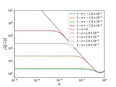
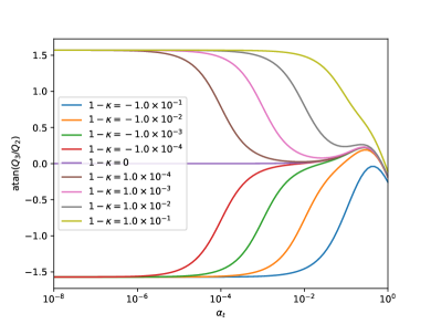
Figure 4: The horizontal torque components for the steady-state particular solution, expressed in terms of Ogilvie’s $Q_{4}=Q_{2}+iQ_{3}$, where $Q_{2}$ and $Q_{3}$ are defined by Eqs. (133, 134). Left: $|Q_{4}|=\sqrt{Q_{2}^{2}+Q_{3}^{2}}$. Right: $\phi_{0}=\mathrm{arg}(Q_{4})=\mathrm{atan}(Q_{3}/Q_{2})$.

In Fig. 4 the $|Q_{4}|$ and $\phi_{0}$ are shown. This figure also makes clear the resonant behavior of the torque: For $\kappa\rightarrow 1$ and for $\alpha_{t}\rightarrow 0$ the amplitude tends to infinity. Physically the warp is like a oscillator with natural dimensionless frequency $\kappa$, driven by the warp at dimensionless frequency $1$. When $\kappa$ approaches unity, the oscillator approaches the resonance, and only viscous damping can prevent it from becoming infinite.

For the special case $\kappa=1$ (i.e. $\epsilon=0$) we find:

$$Q_{1} = -q\alpha_{t}$$ (141)

$$Q_{2} = \left(\frac{1+7\alpha_{t}^{2}}{4+\alpha_{t}^{2}}\right)\,\frac{1}{\alpha_{t}}$$ (142)

$$Q_{3} = \left(\frac{\tfrac{3}{2}-3\alpha_{t}^{2}}{4+\alpha_{t}^{2}}\right)$$ (143)

which are identical to Eqs. (95, 97, 98) of Ogilvie & Latter (2013a). This was to be expected, since we use the same framework. For the special case that both $0<\alpha_{t}\ll 1$ and $0<|\kappa-1|\ll 1$ we have:

$$Q_{1} = -q\alpha_{t}$$ (144)

$$Q_{2} \simeq \frac{\alpha_{t}}{(\kappa^{2}-1)^{2}+4\alpha_{t}^{2}}$$ (145)

$$Q_{3} \simeq -\frac{\tfrac{1}{2}(\kappa^{2}-1)-\tfrac{3}{2}\alpha_{t}^{2}}{(\kappa^{2}-1)^{2}+4\alpha_{t}^{2}}$$ (146)

This limit is of particular interest to protoplanetary discs, where it is thought that the viscosity is low, and the deviations from Keplerian rotation ($\kappa\neq 1$, $\epsilon\neq 0$) are caused by the radial pressure gradient.

6.2 The role of the homogeneous solution of the sloshing motion

Let us now insert the full (particular+homogeneous) solution of $V_{x}(\tau)$ into the internal torque components:

$$2G_{X}/g_{0} = -(V_{xp0}+i\alpha_{t}V_{xp0}+\alpha_{t}\psi)$$ (147)

$$-(V_{xh0}+i\alpha_{t}V_{xh0})e^{i\omega_{0}\tau}$$

$$2G_{Y}/g_{0} = -(iV_{xp0}-\alpha_{t}V_{xp0}+i\alpha_{t}\psi)$$ (148)

$$-(iV_{xh0}-\alpha_{t}V_{xh0})e^{i\omega_{0}\tau}$$

$$G_{Z}/g_{0} = q\alpha_{t}$$ (149)

with $V_{xh0}=V_{x0}-V_{xp0}$ where $V_{x0}$ is the initial condition of the sloshing motion (a complex number), and $\omega_{0}=\kappa-1+i\alpha_{t}$ (cf. Eq. 99). This can be re-written as

$$G_{X} = G_{Xp0}+(G_{X0}-G_{Xp0})e^{i\omega_{0}\tau}$$ (150)

$$G_{Y} = G_{Yp0}+(G_{Y0}-G_{Yp0})e^{i\omega_{0}\tau}$$ (151)

$$G_{Z} = g_{0}q\alpha_{t}$$ (152)

where $G_{X0}=G_{X}(\tau=0)$ is the initial condition for $G_{X}(\tau)$, and likewise for the $Y$ component. The “steady-state particular solutions” for the internal torque $G_{Xp0}$ and $G_{Yp0}$ are defined as in Eqs. (123,124) with $V_{x}(\tau)$ set to the steady-state particular solution for the sloshing motion $V_{xp0}$. So now we have expressed $G_{X}(\tau)$ and $G_{Y}(\tau)$ in a similar way as for $V_{x}(\tau)$: as a sum of a steady-state particular solution and a transient homogeneous solution. The dimensionless time scale of the decay of the transient is $1/\alpha_{t}$, and the dimensionless time scale for the rotation of the transient around the steady-state particular solution is $1/|\kappa-1|$.

The interpretation of this result is that the $Q_{1}$, $Q_{2}$ and $Q_{3}$ values determine the internal torque vector if the sloshing motion has reached its steady-state oscillation, i.e. if the homogeneous solution has decayed to zero and only the steady-state particular solution remains. For large $\alpha_{t}$ this is reached in a few orbits, on a time scale shorter than the time scale at which the warp changes. For small $\alpha_{t}$ this steady-state oscillation may never be reached, as the warp may change faster than that. The distinction between the diffusive regime and the wavelike regime of warped discs is then simply whether or not the transient part of ${\bf G}{}$ decays faster or slower than the change of the warp $\psi$.

7 Ordinary differential equation for ${\bf G}{}$

With the results of Section 6.2 we now have a complete description of how ${\bf G}{}(\tau)$ behaves as a function of the warp amplitude $\psi$, dimensionless time $\tau=\Omega_{0}t$ and the initial condition ${\bf G}{}(0)$. However, our solution (Eqs. 150-152) is only valid for a warp $d{\bf l}{}(r)/d\ln r$ that is constant in time. As a result of the torque ${\bf G}{}$, however, the orientations ${\bf l}{}(r)$ of the annuli change, and thereby the warp vector ${\boldsymbol{\psi}}=d{\bf l}{}(r)/d\ln r$ changes as well: both its amplitude $\psi=|{\boldsymbol{\psi}}|$ and its direction ${\bf e}_{\psi}{}={\boldsymbol{\psi}}/\psi$. This introduces two problems:

1. If $\psi$ changes with time, the simple expressions for ${\bf G}(\tau)$, Eqs. (150-152), no longer apply.

2. The orbital plane of the annulus changes, meaning that at a later time we need to perform a coordinate transformation from $(X,Y,Z)$ to the new coordinates $(X^{\prime},Y^{\prime},Z^{\prime})$ where the new orbital plane lies again in the $(X^{\prime},Y^{\prime})$-plane.

Problem 1 can be relatively easily solved by formulating an ordinary differential equation (ODE) for ${\bf G}$ that has Eqs. (150-151) as a solution, as we will describe in Section 7.1. Problem 2 is harder to solve. We will propose a solution to this problem in Section 7.2.

Both solutions rely on the splitting of ${\bf G}$ into a dynamic sloshing torque ${\bf G}^{(s)}$ and a non-dynamic viscous torque ${\bf G}^{(v)}$:

$${\bf G}={\bf G}^{(s)}+{\bf G}^{(v)}$$ (153)

which, in the usual $(X,Y,Z)$ coordinate system, have the following components (see Eqs. 127, 129):

$${\bf G}^{(s)}(\tau)=\frac{g_{0}}{2}\left(\begin{matrix}-V_{x}^{\mathrm{re}}(\tau)+\alpha_{t}V_{x}^{\mathrm{im}}(\tau)\\ V_{x}^{\mathrm{im}}(\tau)+\alpha_{t}V_{x}^{\mathrm{re}}(\tau)\\ 0\end{matrix}\right)$$ (154)

and

$${\bf G}^{(v)}=g_{0}\left(\begin{matrix}-\alpha_{t}\psi\\ 0\\ q\alpha_{t}\end{matrix}\right)$$ (155)

The latter can be expressed in coordinate-free form as follows:

$${\bf G}^{(v)}=g_{0}q\alpha_{t}{\bf l}-g_{0}\alpha_{t}{\boldsymbol{\psi}}$$ (156)

For the dynamic ${\bf G}^{(s)}(\tau)$ we need to set up an ODE, which we do next.

7.1 Solution to problem 1: ODE for the sloshing torque

The most straightforward ODE for the sloshing torque components $G^{(s)}_{X}(\tau)$ and $G^{(s)}_{X}(\tau)$ that has Eqs. (150-151) as a solution is:

$$\partial_{\tau}G^{(s)}_{X}(\tau) = i\omega_{0}\big{(}G^{(s)}_{X}(\tau)-G^{(s)}_{Xp0}\big{)}$$ (157)

$$\partial_{\tau}G^{(s)}_{Y}(\tau) = i\omega_{0}\big{(}G^{(s)}_{Y}(\tau)-G^{(s)}_{Yp0}\big{)}$$ (158)

If $\psi$ changes, then the solution automatically adapts to the changing value of $\psi$. Using $\omega_{0}=\kappa-1+i\alpha_{t}$ and $G^{(s)}_{Y}=iG^{(s)}_{X}$, and taking the real parts of both sides of the equations we obtain:

$$\partial_{\tau}G^{(s)\,\mathrm{re}}_{X}(\tau) = (\kappa-1)\big{(}G^{(s)\,\mathrm{re}}_{Y}(\tau)-G^{(s)\,\mathrm{re}}_{Yp0}\big{)}$$ (159)

$$-\alpha_{t}\big{(}G^{(s)\,\mathrm{re}}_{X}(\tau)-G^{(s)\,\mathrm{re}}_{Xp0}\big{)}$$

$$\partial_{\tau}G^{(s)\,\mathrm{re}}_{Y}(\tau) = -(\kappa-1)\big{(}G^{(s)\,\mathrm{re}}_{X}(\tau)-G^{(s)\,\mathrm{re}}_{Xp0}\big{)}$$ (160)

$$-\alpha_{t}\big{(}G^{(s)\,\mathrm{re}}_{Y}(\tau)-G^{(s)\,\mathrm{re}}_{Yp0}\big{)}$$

where it is important to note the different sign of the first term of the right-hand-side in both equations. This suggests (but see Section 7.2 for an important addition) the following vectorial form of these equations:

$$\frac{\partial{\bf G}^{(s)}}{\partial\tau}=-(\kappa-1){\bf l}\times({\bf G}^{(s)}-{\bf G}^{(s)}_{p0})-\alpha_{t}({\bf G}^{(s)}-{\bf G}^{(s)}_{p0})$$ (161)

where here the ${\bf G}^{(s)}$ is considered to be a real-valued vector, and ${\bf G}^{(s)}_{p0}$ is given by

$${\bf G}^{(s)}_{p0}=-g_{0}\left(Q_{2}\frac{d{\bf l}}{d\ln r}+Q_{3}{\bf l}\times\frac{d{\bf l}}{d\ln r}\right)$$ (162)

with $Q_{2}$ and $Q_{3}$ given by Eqs. (136-137), and $g_{0}\equiv\Omega_{0}^{2}r_{0}\Sigma h_{p}^{2}$ (cf. Eq. 126).

To make it easier to compare our dynamic equation for ${\bf G}^{(s)}$ (Eq. 161) to the literature, we can rewrite it by bringing the ${\bf G}^{(s)}$ terms to the left-hand-side, and keeping the ${\bf G}^{(s)}_{p0}$ terms on the right-hand-side:

$$\frac{\partial{\bf G}^{(s)}}{\partial\tau}+(\kappa-1){\bf l}{}\times{\bf G}^{(s)}+\alpha_{t}{\bf G}^{(s)}=(\kappa-1){\bf l}{}\times{\bf G}^{(s)}_{p0}+\alpha_{t}{\bf G}^{(s)}_{p0}$$ (163)

By inserting the expression for ${\bf G}^{(s)}_{p0}$ (Eq. 162) we obtain

$$\begin{split}\frac{\partial{\bf G}^{(s)}}{\partial\tau}+&(\kappa-1){\bf l}{}\times{\bf G}^{(s)}+\alpha_{t}{\bf G}^{(s)}\\ =&-(\kappa-1)g_{0}\left(Q_{2}{\bf l}{}\times\frac{d{\bf l}{}}{d\ln r}-Q_{3}\frac{d{\bf l}{}}{d\ln r}\right)\\ &-\alpha_{t}g_{0}\left(Q_{2}\frac{d{\bf l}{}}{d\ln r}+Q_{3}{\bf l}{}\times\frac{d{\bf l}{}}{d\ln r}\right)\end{split}$$ (164)

This equation is exactly the same as Eq. (161), just written out more explicitly. For notational convenience let us regroup the terms on the right-hand-side:

$$\begin{split}\frac{\partial{\bf G}^{(s)}}{\partial\tau}+&(\kappa-1){\bf l}{}\times{\bf G}^{(s)}+\alpha_{t}{\bf G}^{(s)}\\ =&-g_{0}\left(\tilde{Q}_{2}\frac{d{\bf l}{}}{d\ln r}+\tilde{Q}_{3}{\bf l}{}\times\frac{d{\bf l}{}}{d\ln r}\right)\end{split}$$ (165)

with

$$\tilde{Q}_{2} = \alpha_{t}Q_{2}-(\kappa-1)Q_{3}$$ (166)

$$\tilde{Q}_{3} = (\kappa-1)Q_{2}+\alpha_{t}Q_{3}$$ (167)

Fig. 5 shows the dependency of $\tilde{Q}_{2}$ and $\tilde{Q}_{3}$ on $\alpha_{t}$ and $\kappa-1$.

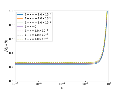
Figure 5: As Fig. 4, but for $\tilde{Q}_{2}$ and $\tilde{Q}_{3}$, which are the coefficients entering the time-dependent equation for the torques, Eq. (165), where $\tilde{Q}_{2}$ and $\tilde{Q}_{3}$ are defined by Eqs. (166, 167). Left: $|\tilde{Q}_{4}|=\sqrt{\tilde{Q}_{2}^{2}+\tilde{Q}_{3}^{2}}$. Right: $\tilde{\phi}_{0}=\mathrm{arg}(\tilde{Q}_{4})=\mathrm{atan}(\tilde{Q}_{3}/\tilde{Q}_{2})$.

In the limit of $\alpha_{t}\ll 1$ and $|\kappa-1|\ll 1$ we find that

$$\tilde{Q}_{2}\rightarrow\frac{1}{4},\qquad\frac{\tilde{Q}_{3}}{\tilde{Q}_{2}}\rightarrow 0$$ (168)

so that, in this limit, our equation simplifies to

$$\frac{\partial{\bf G}^{(s)}}{\partial\tau}+(\kappa-1){\bf l}{}\times{\bf G}^{(s)}+\alpha_{t}{\bf G}^{(s)}\simeq-\frac{g_{0}}{4}\frac{d{\bf l}{}}{d\ln r}$$ (169)

This equation is identical to Eq. (13) of Lubow & Ogilvie (2000) if we set the total torque to be the sloshing torque ${\bf G}={\bf G}^{(s)}$ (neglecting the viscous torque for reasons that $\alpha_{t}\ll 1$), and define

$$\omega_{a}\equiv\frac{\kappa^{2}-1}{2}\simeq\kappa-1$$ (170)

where the last step is approximately valid for $|\kappa-1|\ll 1$.

7.2 Solution to problem 2: Rotating ${\bf G}^{(s)}$

Problem 2 is harder to solve, because it requires knowledge about if and how ${\bf G}^{(s)}$ changes when the orbital plane changes, i.e. when ${\bf l}$ changes. If we look again at the individual components of ${\bf G}^{(s)}$ given in Eq. (154), we see that the nature of ${\bf G}^{(s)}$ is fundamentally fixed to the orientation of the orbital plane. The sloshing motion, and thereby the sloshing torque, is strictly in the plane of the disc (the $X$-$Y$-plane), or in other words: ${\bf G}^{(s)}\cdot{\bf l}=0$. If the orientation of the orbital plane changes, i.e. $d{\bf l}/d\tau\neq 0$, and if we leave the 3-D orientation of ${\bf G}^{(s)}$ unchanged, then in the new coordinates $(X^{\prime},Y^{\prime},Z^{\prime})$, which describe the new orbital plane, we will see $G^{(s)}_{X}$ and $G^{(s)}_{Y}$ rotationally mix into $G^{(s)}_{Z^{\prime}}$. This means that the latter becomes non-zero, and the condition ${\bf G}^{(s)}\cdot{\bf l}=0$ is broken. This is illustrated in Fig. 6.

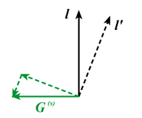
Figure 6: Cartoon of how the in-plane sloshing torque acquires a perpendicular component upon a change of the orientation vector of the orbital plane ${\bf l}\rightarrow{\bf l}^{\prime}$. Solid lines: before the change, dashed lines: after the change, at which point ${\bf G}^{(s)}$ has acquired a ${\bf G}^{(s)}\cdot{\bf l}^{\prime}\neq 0$ component. This “leakage” of the sloshing torque into the perpendicular viscous torque can quickly dominate over the true perpendicular viscous torque ${\bf G}^{(v)}$, and can unphysically affect the viscous evolution of $\Sigma(r,t)$.

Given that the sloshing torque is usually orders of magnitude larger than the viscous torque ($|G^{(s)}|\gg|G^{(v)}|$), even a comparatively small non-zero $G^{(s)}_{Z^{\prime}}$ can easily dominate the much smaller perpendicular viscous torque $G^{(v)}_{Z^{\prime}}=g_{0}q\alpha_{t}$. So this “leakage” of the sloshing torque into the perpendicular torque component is not harmless: It can strongly affect the perpendicular component of ${\bf G}={\bf G}^{(s)}+{\bf G}^{(v)}$ (i.e. the value of ${\bf G}\cdot{\bf l}$), which is responsible for the radial accretion of the disc material. This can therefore lead to strange effects in the evolution of $\Sigma(r,t)$, as is demonstrated in Martin et al. (2019), their Fig. (1, upper right panel), and will be further discussed in Section 8.1.

The question is now: Is this “pollution” of the ${\bf G}\cdot{\bf l}$ component by the sloshing torque physical or not? If it is physical, then it should be possible to find a sloshing motion that produces a non-zero component of ${\bf G}^{(s)}$ in the direction of ${\bf l}$. At least in the linear regime, and assuming that $v_{i}^{\prime}(z^{\prime})=V_{i}\Omega_{0}z^{\prime}$ (cf. Eqs. 43-45), no such motion can be found, because under these conditions the general form of the torque is given by Eqs. (123-125), which does not have a component of $V$ in the expression for ${\bf G}_{Z}$.

Assuming that this holds also in the non-linear regime, we can say that when ${\bf l}$ changes, the sloshing torque ${\bf G}^{(s)}$ changes as well, such that ${\bf G}^{(s)}\cdot{\bf l}$ stays zero at all times.

We conjecture at this point that the sloshing torque ${\bf G}^{(s)}$ is simply co-rotated with the change (i.e. rotation) of ${\bf l}$. The rotation-per-unit-dimensionless-time is defined by two vectors, ${\bf l}$ and $d{\bf l}/d\tau$. Together they define a rotation axis ${\bf R}\equiv{\bf l}\times d{\bf l}/d\tau$. Using Rodrigues’ formula in the limit of infinitesimal rotations we find that the rotation of ${\bf G}^{(s)}$ is given by

$$\frac{\partial{\bf G}^{(s)}}{\partial\tau}=\left({\bf l}\times\frac{d{\bf l}}{d\tau}\right)\times{\bf G}^{(s)}$$ (171)

Putting it all together, we add the rotation term of Eq. (171) to the evolution equation for ${\bf G}^{(s)}$ (Eq. 164, or Eq. 169 in the limit of small $\alpha_{t}$ and $|\kappa-1|$), and we obtain the full evolution equation for ${\bf G}^{(s)}$ which avoids the unphysical “leakage” of the sloshing torque into the perpendicular torque component. The general result is:

$$\begin{split}\frac{\partial{\bf G}^{(s)}}{\partial\tau}+&(\kappa-1){\bf l}{}\times{\bf G}^{(s)}+\alpha_{t}{\bf G}^{(s)}\\ =&-g_{0}\left(\tilde{Q}_{2}\frac{d{\bf l}{}}{d\ln r}+\tilde{Q}_{3}{\bf l}{}\times\frac{d{\bf l}{}}{d\ln r}\right)\\ &+\left({\bf l}\times\frac{d{\bf l}}{d\tau}\right)\times{\bf G}^{(s)}\end{split}$$ (172)

In the limit of small $\alpha_{t}$ and $|\kappa-1|$ this simplifies to (cf. Eq. 169):

$$\begin{split}\frac{\partial{\bf G}^{(s)}}{\partial\tau}&+(\kappa-1){\bf l}{}\times{\bf G}^{(s)}+\alpha_{t}{\bf G}^{(s)}\\ &\simeq-\frac{g_{0}}{4}\frac{d{\bf l}{}}{d\ln r}+\left({\bf l}\times\frac{d{\bf l}}{d\tau}\right)\times{\bf G}^{(s)}\end{split}$$ (173)

The total torque, at each moment in time, is then

$${\bf G}={\bf G}^{(s)}+{\bf G}^{(v)}={\bf G}^{(s)}+qg_{0}\alpha_{t}{\bf l}-g_{0}\alpha_{t}{\boldsymbol{\psi}}$$ (174)

where ${\bf G}^{(s)}$ is the solution of Eq. (172) or Eq. (173), and where we used Eq. (156) in the final step.

Together with the global mass and angular momentum equations (see Section 3) the above equations for ${\bf G}{}(\tau)$ (Eqs. 172/173, 174) forms a full set of dynamic equations for the evolution of a warped disc in the limit of small $\alpha_{t}$. They unify the diffusive and wave-like regime.

It should be kept in mind, however, that the rotational behavior of ${\bf G}^{(s)}$ according to Eq. (171) is a conjecture. It makes intuitive sense, and it removes an unphysical property of the previous equations, but in itself it remains unproven.

The extra rotational term in Eq. (173) is not seen in the equations of Ogilvie (1999); Lubow & Ogilvie (2000). Given that these papers were not concerned with the co-evolution of $\Sigma(r,t)$, they were not concerned with the ${\bf G}^{(s)}\cdot{\bf l}$ component of their torque. Since

$${\bf G}^{(s)}\cdot\left({\bf l}\times\frac{d{\bf l}}{d\tau}\right)\times{\bf G}^{(s)}=0$$ (175)

this term, at least in the limit of small warps, does not affect their results for the wavelike propagation of the warp. But it is important when, in addition, the viscous evolution of $\Sigma(r,t)$ is considered.

When using Eq. (172) or Eq. (173) in a numerical integration algorithm, it should, however, be kept in mind that even the slightest numerical error in the rotation may still “leak” too much of the sloshing torque into the perpendicular torque component. This is because, for small $\alpha_{t}$, the magnitude of the in-plane sloshing torque is so much larger than the perpendicular viscous torque. In practice it may therefore improve the stability and reliability of the algorithm to “reset” the perpendicular component of the sloshing torque to zero every time step:

$${\bf G}^{(s)}:={\bf G}^{(s)}-({\bf G}^{(s)}\cdot{\bf l}){\bf l}$$ (176)

In fact, numerical experimentation shows (see Section 8.1) that this “resetting trick” is so effective for sufficiently small time steps, that the rotational term is no longer strictly needed: the “resetting” does the rotation automatically. This is because the rotational term is perpendicular to the orbital plane, and thus perpendicular to the sloshing torque (as is true for any infinitesimal rotation). The numerical errors in the orbital plane are quadratic in the rotation angle, and thus become vanishingly small for sufficiently small time steps.

7.3 Alternative solution to problem 2: Martin’s $\beta$ terms

Martin et al. (2019) choose a different path to overcome the “leakage” problem. They do not distinguish between the sloshing torque ${\bf G}^{(s)}$ and the viscous torque ${\bf G}^{(v)}$, but instead add a strong damping term to their equation for $\partial{\bf G}/\partial\tau$ that forces the ${\bf G}\cdot{\bf l}$ component to converge to the correct value on a short time scale. This time scale $\tau_{\mathrm{damp}}=1/\beta$, with $\beta$ the proportionality parameter of their damping term, can be chosen at will. The shorter this damping time scale (i.e. the larger $\beta$), the better the artificial “leakage” is suppressed, but at the cost of the equations becoming more stiff and thus harder to solve numerically.

Let us derive their equation starting from our Eqs. (161, 162) but with ${\bf G}^{(s)}$ replaced by ${\bf G}$

$$\frac{\partial{\bf G}}{\partial\tau}=-(\kappa-1){\bf l}\times({\bf G}-{\bf G}_{p0})-\alpha_{t}({\bf G}-{\bf G}_{p0})$$ (177)

and with ${\bf G}_{p0}$ given by

$${\bf G}_{p0}=-g_{0}\left(Q_{1}{\bf l}+Q_{2}\frac{d{\bf l}}{d\ln r}+Q_{3}{\bf l}\times\frac{d{\bf l}}{d\ln r}\right)$$ (178)

(instead of Eq. 162). In other words, the ${\bf G}\cdot{\bf l}$ component is now included in the equation, and the $Q_{1}{\bf l}$ term on the right-hand-side ensures that the ${\bf G}\cdot{\bf l}$ dynamically converges to the correct value $g_{0}q\alpha_{t}$ over a time scale $1/\alpha_{t}$. Following the same path as before, we can derive the equivalent of Eq. (165)

$$\begin{split}\frac{\partial{\bf G}}{\partial\tau}+&(\kappa-1){\bf l}{}\times{\bf G}+\alpha_{t}{\bf G}\\ =&-g_{0}\left(\tilde{Q}_{1}{\bf l}+\tilde{Q}_{2}\frac{d{\bf l}{}}{d\ln r}+\tilde{Q}_{3}{\bf l}{}\times\frac{d{\bf l}{}}{d\ln r}\right)\end{split}$$ (179)

where $\tilde{Q}_{1}=\alpha_{t}Q_{1}$, and the $\tilde{Q}_{2}$ and $\tilde{Q}_{3}$ are defined by Eqs. (166, 167). Following the same reasoning as before, we arrive, for small $\alpha_{t}$ and $|\kappa-1|$, at the equivalent of Eq. (169)

$$\frac{\partial{\bf G}}{\partial\tau}+(\kappa-1){\bf l}{}\times{\bf G}+\alpha_{t}{\bf G}\simeq g_{0}q\alpha_{t}^{2}\;{\bf l}-\frac{g_{0}}{4}\frac{d{\bf l}{}}{d\ln r}$$ (180)

This is the equivalent of Martin et al. (2019)’s Equation (15), without their $\beta$-terms. If ${\bf l}$ changes very slowly with time, then Eq. (180) assures that the ${\bf G}\cdot{\bf l}$ component dynamically converges to the correct value. In principle this convergence also automatically damps away any “leaked” sloshing torque, but the time scale of $\tau_{\mathrm{damp}}=1/\alpha_{t}\gg 1$ is much too long to suppress this leakage. To ameliorate this, Martin et al. (2019) add two terms to their equation:

$$\begin{split}\frac{\partial{\bf G}}{\partial\tau}&+(\kappa-1){\bf l}{}\times{\bf G}+\alpha_{t}{\bf G}+\beta({\bf G}\cdot{\bf l}){\bf l}\\ &=g_{0}q\alpha_{t}(\alpha_{t}+\beta)\;{\bf l}-\frac{g_{0}}{4}\frac{d{\bf l}{}}{d\ln r}\end{split}$$ (181)

For values of $\beta\gg|d{\bf l}/d\tau|^{-1}$ we can estimate the behavior of the perpendicular torque component ${\bf G}\cdot{\bf l}$ by taking the inner product of this equation with ${\bf l}$:

$$\frac{\partial({\bf G}\cdot{\bf l})}{\partial\tau}+(\alpha_{t}+\beta){\bf G}\cdot{\bf l}=g_{0}q\alpha_{t}(\alpha_{t}+\beta)$$ (182)

where we neglected the ${\bf G}\cdot d{\bf l}/d\tau$ term. The solution to this equation is the usual exponential convergence to the value

$${\bf G}\cdot{\bf l}\rightarrow g_{0}q\alpha_{t}$$ (183)

and the time scale is $\tau_{\mathrm{damp}}=1/(\alpha_{t}+\beta)$. Martin et al. (2019) report values of $\beta\gtrsim 10$ to lead to reasonably good results.

In the hypothetical limit of $\beta\rightarrow\infty$ this method always guarantees that ${\bf G}\cdot{\bf l}=g_{0}q\alpha_{t}$, or equivalently that ${\bf G}^{(s)}\cdot{\bf l}=0$ at all times. In an explicit numerical integration algorithm this can, alternatively, be achieved by applying the “resetting condition” Eq. (176) at each time step. This avoids the numerical stiffness problem for large $\beta$ values, and achieves the same effect as the $\beta$-terms in Eq. (181), as will be discussed in Section 8.1.

8 Discussion

8.1 Numerical analysis of the behavior of the equations

To investigate the behavior of our new equations, we perform the same test calculation as presented by Martin et al. (2019) in their Section 4. It is a dimensionless setup, with a disk ranging from $r_{\mathrm{in}}=1$ to $r_{\mathrm{out}}=20$, with a surface density that has smooth cut-offs at both the inner and outer radius, and a warp of 10 degrees, given by the equation (see Martin et al., 2019)

$$\Sigma(r,t=0)=\Sigma_{0}\left(\frac{r}{r_{\mathrm{in}}}\right)^{-p}\left[1-\left(\frac{r_{\mathrm{in}}}{r}\right)^{1/2}\right]\left[1-e^{r-r_{\mathrm{out}}}\right].$$ (184)

Here, $\Sigma_{0}$ is a scaling constant and can be chosen arbitrarily. Initially, the disk is only warped in one direction (‘untwisted’) and remains that way throughout the simulations. This is due to the absence of precession terms in the equations we use. Therefore, the initial shape of the disk can be determined by the inclination angle $i$ which is the angle between the local orbital plane and the $x$-$y$–plane. We set the initial inclination profile to (see Martin et al., 2019)

$$i(r,t=0)=10\textdegree\left[\frac{1}{2}\tanh\left(\frac{r-r_{\mathrm{warp}}}{r_{\mathrm{width}}}\right)+\frac{1}{2}\right],$$ (185)

with the location of the warp $r_{\mathrm{warp}}=10$ and the warp width $r_{\mathrm{width}}=2$. At the start of the calculation, ${\bf G}(r,t=0)$ is set to the viscous torque ${\bf G}^{(v)}(r)$, i.e. the sloshing torque is set to zero. The viscosity is set to $\alpha_{t}=0.01$ and the disc aspect ratio is set to $H_{p}/r=0.1$.

The procedure for the numerical integration method of our generalized warped disc equation is described in Section 8.5.

We integrate until dimensionless time 2000, which is roughly one wave-crossing time for the warp. We carry out these calculations in five different ways, from left to right in Fig. 7:

1. In the first calculation, we use use the equations of Martin et al. (2019), with $\beta=0$. This is equal to our equations without the rotation term (i.e. without the $({\bf l}\times d{\bf l}/d\tau)\times{\bf G}$ term). This calculation shows what goes wrong when the ${\bf G}\cdot{\bf l}$ component of the internal torque is left “untreated”. The surface density acquires a strong wiggle, first identified by Martin et al. (2019), which is not seen in 3-D hydrodynamic simulations of warped discs (e.g. Nealon et al., 2015). We also see a strong effect on the inner edge of the disc, which is equally suspicious. In the bottom panel the cause of these phenomena can be seen. The ${\bf G}\cdot{\bf l}$ component should, physically, be just the viscous torque. Yet, the “leakage” of the sloshing torques into this perpendicular component of ${\bf G}$ completely overpowers the viscous torque, and even causes (inward of a radius of 10 to 20 code units) a negative torque. This de-facto acts as a negative viscosity, and thus violates the second law of thermodynamics. It must therefore be an unphysical effect.

2. The same, but now with $\beta=10$, to damp the ${\bf G}\cdot{\bf l}$ component back to what it should be: ${\bf G}\cdot{\bf l}\rightarrow{\bf G}^{(v)}\cdot{\bf l}$. Apart from small deviations this is indeed successful. The remaining “triangle like” curve is the expected curve for the viscous ${\bf G}^{(v)}\cdot{\bf l}$. As a result, no spurious features appear in the $\Sigma(r,t)$. The remaining viscous evolution (very minor effects on these time scales) are physical.

3. The same, but now with $\beta=100$, i.e. even stronger damping. The small remaining deviations from ${\bf G}^{(v)}\cdot{\bf l}$ are nearly gone. Both this and the $\beta=10$ case demonstrate that the method of Martin et al. (2019) indeed works as advertised. However, a large $\beta$ makes the equations stiff and thus harder to solve numerically.

4. Instead of using the $\beta$ damping, we reset ${\bf G}\cdot{\bf l}\rightarrow{\bf G}^{(v)}\cdot{\bf l}$ after each time step. This is also succesful, and achieves the same result as for $\beta=100$.

5. Finally, including the rotational term to the equation (last term of Eq. 173), but without $\beta$ and without resetting. One can see that ${\bf G}\cdot{\bf l}$ does not have any “leakage” of the sloshing torque into the perpendicular torque, and it is even closer to the correct value, without any damping or resetting.

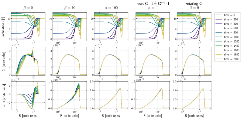
Figure 7: Results of the test model of Martin et al. (2019) for five different methods of handling the ${\bf G}\cdot{\bf l}$ component of the internal torque (from left to right). In the first four, the equations of Martin et al. (2019) are used. In the fourth panel, $\beta$ is again 0, but the ${\bf G}\cdot{\bf l}$ component is reset to the correct value ${\bf G}^{(v)}\cdot{\bf l}$ after each macroscopic time step (i.e. not during the sub-timestepping done by the odeint integrator of scipy). In the final panel, the rotation term is added to the equation for ${\bf G}$ (final term in Eq. 173), which is the equation proposed in this paper. Top row: the inclination $i$ in degrees. Middle row: the surface density $\Sigma(r,t)$. Bottom row: the ${\bf G}\cdot{\bf l}$.

We conclude that our equation (Eq. 173) with the rotation term, possibly with an occasional “reset”, is the most physically consistent equation for ${\bf G}$ for modeling the evolution of a warped disc.

8.2 Shearing box versus tilted slab interpretation

The fact that the sloshing motion causes an internal torque is known since Papaloizou & Pringle (1983). However, the physics behind this fact is not intuitively obvious. In the top row of Fig. 8 the case of pure warp-damping ($\phi_{0}=0$) without twisting is pictographically shown. In this porous shearing box picture, the torque is entirely due to angular momentum advected between adjacent annuli (here shown in blue and orange) by the horizontal velocity $v_{x}^{\prime}(z^{\prime})$. Gas pressure plays no role from this point of view, because the box walls are vertical, so that the blue box cannot exert a vertical force on the orange box and vice versa. The derivations in this paper were done in this porous shearing box framework.

In the bottom row of Fig. 8 the exact same situation is depicted from a Lagrange perspective (see the affine model of Ogilvie, 2018). Here, the annuli are not porous, but get tilted by the horizontal velocity $v_{x}^{\prime}(z^{\prime})$. The advective transport of angular momentum no longer plays a role. Instead, the angular momentum exchange between the blue and the orange annuli is now entirely mediated by the pressure, because due to the tilt, the pressure now causes the two annuli to extert a vertical force on each other.

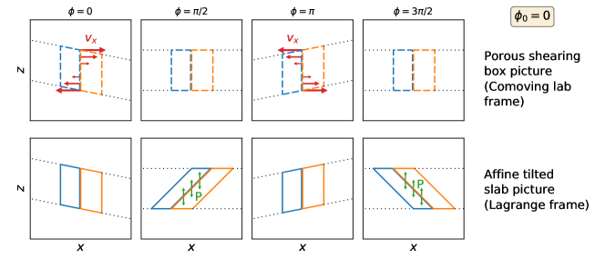
Figure 8: Cartoon of the sloshing motion for the case $\phi_{0}=0$ ($Q_{2}>0$, $Q_{3}=0$), i.e. pure warp-damping, without twisting. Two interpretations are shown. Top row: The comoving lab frame picture, which is the way by which all equations in this paper have been derived (using a porous shearing box). The red arrows show the radial velocity $v_{x}^{\prime}(z)$ of the gas, transporting angular momentum between the blue and the orange annuli. Bottom row: The Lagrange picture, in which the slabs (annuli) are tilted due to the horizontal sloshing motion (see the affine tilted slab model of Ogilvie (2018)). The green arrows show the vertical pressure force exchange, which lead to a torque that the blue and the orange annuli exert on each other. The cartoons are qualitative, and not to scale.

To show that the two perspectives are equivalent, we can compute the tilt angle $\theta$ as a function of $\tau$. Comoving with the orbital motion, it obeys the following ODE:

$$\frac{d\tan\theta(\tau)}{d\tau}=V^{\mathrm{re}}_{x}(\tau)$$ (186)

If $V_{x}(\tau)$ is the $m=1$ periodic solution, then in the $(\tau,\phi)$-picture (see Section 5.3), the $\tau$-coordinate is replaced by the $\phi$ coordinate. So the above differential equation in $\tau$ becomes the same differential equation in $\phi$. Given that the $m=1$ mode goes as $e^{i\phi}$, the solution is:

$$\tan\theta(\phi)=\mathrm{Re}[-iV_{x}(\phi)]=V^{\mathrm{im}}_{x}(\phi)$$ (187)

where we set the integration constant to zero. Here $\theta=0$ means the slab is vertical and $\theta>0$ means the slab is tilted clockwise, i.e. $\tan\theta=x/z$ for a gas parcel belonging to the slab going through $(x,z)=(0,0)$. With a non-zero tilt, the gas pressure acquires the possibility to transport $z$-momentum in $z$ direction from one slab to the next. In other words, neighboring tilted slabs can exchange $y$-angular momentum with each other through the pressure force. The internal torque is defined as the transmission of angular momentum from one slab at $r_{0}$ to its neighbor at $r_{0}+\Delta r$:

$$\begin{split}\bar{g}_{y}&=r_{0}\int_{-\infty}^{\infty}p(z^{\prime})\tan(\theta)dz^{\prime}\\ &=\Omega_{0}^{2}r_{0}\Sigma h_{p}^{2}\tan(\theta(\phi))\equiv g_{0}\tan(\theta(\phi))\equiv g_{0}V^{\mathrm{im}}_{x}(\phi)\end{split}$$ (188)

In complex notation we thus have

$$\bar{g}_{y}(\phi)=-ig_{0}V_{x}(\phi)$$ (189)

and $\bar{g}_{x}=0$. Inserting these into Eqs. (117, 118) and the results into Eqs. (120, 121), following the method outlined in Appendix B.5, gives

$$2G_{X}/g_{0} = -V_{x}(\tau)$$ (190)

$$2G_{Y}/g_{0} = -iV_{x}(\tau)$$ (191)

which reproduces the same results as for the comoving lab-frame (porous shearing box) analysis (Eqs. 123, 124) in the limit $\alpha_{t}\ll 1$.

For perfectly keplerian discs ($q=1.5$) the amplitude of the tilting (for the case of strong viscous damping) is greatest at $\phi\simeq\pi/2$ and $\phi\simeq 3\pi/2$, as illustrated in Fig. 8. A 3-D version of this is shown in Fig. 9. This means that the pressure-driven torque acts as an $X$-torque and thus damps the warp in this case.

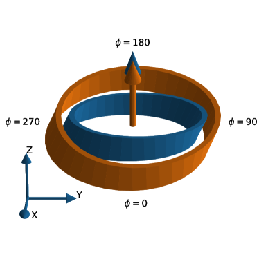
Figure 9: A 3-D rendering of the sloshing / tilting motion shown in Fig. 8 (i.e. for $\phi_{0}=0$, a purely damping torque), shown for two adjacent slabs, following the “affine tilted slab” approach of Ogilvie (2018). The inner blue slab is at $x=0$ and is thus not inclined. The outer orange slab is at $x>0$ and is inclined with respect to the blue slab. The large arrows are the ${\bf l}$ unit vectors for the blue and orange annulus, respectively. The orbital motion is counter-clockwise when seen from above (right-hand rule). Model parameters are: $q=1.5$, $\psi=0.1$ and $\alpha_{t}=0.1$. The maximum tilting of the slabs is at $\phi=\pi/2$ and $\phi=3\pi/2$, and therefore the torque damps the warp.

Twisting torques ($Q_{3}\neq 0$) can appear if the sloshing motion is phase-shifted with respect to the pure damping case ($\phi_{0}\neq 0$). This leads to a shift in the location $\phi$ along the annulus where the tilt is maximal, and thus a rotation of the ${\bf G}$ vector around the ${\bf l}$ vector by an amount $\phi_{0}$. This leads to non-zero $G_{Y}$, which twists the disc.

8.3 Caveats of the model

While the equations for warped disks discussed in this paper are easy to use and numerically cheap to integrate, they have strong limitations. First, they assume that all orbits are circular. Eccentricity can in principle be included (see e.g. Lynch & Ogilvie, 2021), but that requires also a treatment of the disk variables along each orbit, making the model essentially 2-D. There are also other reasons why a 2-D treatment (in the coordinates $r$ and $\phi$) may be necessary. For instance, any out-of-plane companion (planet or binary companion) that induces the warp in the disk may also induce $m=2$ waves (spirals) or higher modes in the disk that may be of equal importance as the warp itself. A treatment similar to the 2-D affine model of Ogilvie (2018) may be necessary to overcome these limitations without directly resorting to 3-D models.

A further major caveat is that the equations of this paper are not capable of treating the breaking of a warped disk. It has been found in many 3-D simulations that under certain conditions the disk cannot maintain a smooth continuous shape, but instead will break into two (or more) disconnected disks (Larwood & Papaloizou, 1997; Lodato & Price, 2010; Fragner & Nelson, 2010; Nixon & King, 2012; Nixon et al., 2013; Facchini et al., 2013; Nealon et al., 2016; Raj et al., 2021). This phenomenon likely requires a fully 3-D treatment.

On the other hand, for computational feasibility, fully global 3-D models of warped disks necessarily have limited numerical resolution at the disk interior scale, i.e. at spatial scales smaller than the pressure scale height. At low viscosity, the strong sloshing motion induced by even small warps can induce turbulence (Kumar & Coleman, 1993; Ogilvie & Latter, 2013b) that may be stronger than the background turbulence (Torkelsson et al., 2000). A local 2-D or 3-D shearing box calculation such as by Paardekooper & Ogilvie (2019) can, however, be used to update the local turbulent viscosity coefficient $\alpha_{t}$, which might then be used in the 1-D warped disk equations again. Whether a simple analytic “fitting formula” can be found for this self-induced turbulent viscosity is not yet clear.

Finally there is the issue of irradiation. For disks around black holes or neutron stars the radiation pressure of this radiation may be strong enough to induce and enhance warping of a disk (Pringle, 1996) and cause precession (Ogilvie & Dubus, 2001). But even for less strong irradiation: the warp causes the disk to be irradiated from one side only, switching side each half orbit. This issue has been studied very recently in the context of the chemistry (Young et al., 2021), but to our knowledge it has not yet been investigated if it affects the internal dynamics of the disk and thus affects the internal torque.

8.4 Applications of the model

One of the reasons why the two regimes of warped disk dynamics have traditionally been treated separately is because accretion disks around black holes and neutron stars are usually geometrically very thin ($h_{p}\ll r$) and hot ($T\gg 1000\,\mathrm{K}$) so that they are firmly in the diffusive regime ($\alpha_{t}>h_{p}/r$). This is because for sufficiently ionized disks the magnetohydrodynamics is nearly ideal, and the saturated magnetorotational turbulence reaches values of the order of $\alpha_{t}\sim 10^{-2}\cdots 10^{-1}$ (e.g. Meheut et al., 2015). Protoplanetary disks, on the other hand, are relatively cold ($T\lesssim 1500\,\mathrm{K}$ in the dusty outer parts) and geometrically not very thin ($h_{p}/r\sim 0.05$). They may thus be much less turbulent than hot disks. The precise value of $\alpha_{t}$ in those disks is still a matter of active debate, (see Lesur et al., 2022), but values of the order of $\alpha_{t}\sim 10^{-4}$ are often suggested, which would put protoplanetary disks firmly in the wavelike regime.

However, at early times and close enough to the star, protoplanetary disks are likely to be much hotter, and fully saturated magnetorotational turbulence ($\alpha_{t}\sim 10^{-2}\cdots 10^{-1}$) should be expected, putting these regions of the protoplanetary disk right in between the two regimes, where the unified set of equations have to be used. Furthermore, as discussed in Section 8.3, the vertical shear instability driven by the sloshing motion may induce strong turbulence, perhaps even stronger than the “traditional” vertical shear instability (VSI) driven by the baroclinic structure of flat disks (Arlt & Urpin, 2004; Nelson et al., 2013; Stoll & Kley, 2014). It is not yet clear if these instabilities may lead to $\alpha_{t}$ of the order of $h_{p}/r$, but if they do, then again, we would be in between the two regimes.

And even if the disk is in the wavelike regime, this does not mean that the viscous radial transport of mass within the disk is not important. The warp waves have a short timescale for travelling through the disk, given that their phase velocity is $c_{s}/2$ (Nelson & Papaloizou, 1999). However, the life time of these disks is much longer, and during that time the viscous evolution of the surface density $\Sigma$ is likely to be non-negligible. If the warp continues to be driven, for instance by a companion, then the warp dynamics and viscous radial mass redistribution have to be treated simultaneously. This required the use of the generalized warp equations.

When applying the equations to protoplanetary disks, it becomes important to be able to include external torques from companions (stars or planets) onto the disk. This can be done in the usual way by adding an external torque ${\bf T}{}$ to the angular momentum conservation equation (Eq. 3), for instance using the equations from Eggleton & Kiseleva-Eggleton (2001), (see also e.g. Liu et al., 2015; Zanazzi & Lai, 2018a). However, this torque will change the orbital orientation ${\bf l}$ of the annuli of the disk, leading to the same “leakage” problem as we discussed in Section 7 (“problem ii”). The solution is then the same as before: rotating ${\bf G}^{(s)}$ such that it stays in the plane. In other words, the $d{\bf l}/d\tau$ in the rotational terms in Eq. (172 or 173) now should include the change of ${\bf l}$ due to the external torque ${\bf T}{}$.

8.5 Numerical recipe for modeling warped discs

Given the complexity of the mathematical description of viscously evolving warped discs, as described in this paper, we here summarize our recommended set of equations and a method of solution for modeling the dynamics of warped discs.

1. The main conservation equation to solve is the equation of angular momentum conservation Eq. (3).

2. Conservation of mass is given by Eq. (1), but this equation is not explicitly needed. The reason is because once we know the angular momentum density ${\bf L}(r,t)$, we can use Eq. (2) to compute the surface denisty $\Sigma(r,t)$ and the unit vector ${\bf l}(r,t)$, because the Kepler frequency $\Omega(r)$ is known. Deviations from Keplerian rotation are not considered here. Optionally one can solve the mass conservation equation in addition to the angular momentum conservation. This leads to a redundancy (see Eq. 2), which can then serve as an indicator of the magnitude of the numerical error made.

3. The torque vector ${\bf G}(r,t)$ is given by Eq. (174), where ${\bf G}^{(s)}(r,t)$ obeys Eq. (172).

4. The values of $\tilde{Q}_{2}$ and $\tilde{Q}_{3}$ are obtained from Eqs. (166, 167), which depend on $Q_{2}$ and $Q_{3}$, the values of which are obtained from Eqs. (136, 137). For small values of $\alpha_{t}$ and $|\kappa-1|$ one can, instead, use the values $\tilde{Q}_{2}=1/4$ and $\tilde{Q}_{3}=0$.

5. The value for $g_{0}$ is given in Eq. (126).

6. The symbol $q$ is defined in Eq. (7), and $\kappa$ is defined in Eq. (73).

7. The dimensionless time $\tau$, used in the above equations, is defined by Eq. (36).

Numerically one can make a linearly or logarithmically spaced grid in $r$ with $N_{r}$ grid points, and on each grid point one places 6 variables: ${L}_{X}$, ${L}_{Y}$, ${L}_{Z}$, $G_{X}$, $G_{Y}$, $G_{Z}$ (or 7 variables, if one opts to include $\Sigma$ as mentioned above), where here the coordinate system $(X,Y,Z)$ can be freely chosen (i.e. it is not necessarily aligned with the warp, as it was during the derivation of the equations). This gives, at each time step, $6N_{r}$ variables. Given that the equations for ${L}_{i}$ are conservation equations, they are best discretized in finite volume conserved form. The equations for $G_{i}$ are strictly local equations (no spatial derivatives involved). They are best formulated at a staggered mesh (grid point in between those of ${L}_{i}$), although also a co-spatial gridding for ${L}_{i}$ and $G_{i}$ is possible. An explicit integration of these equations sets the usual time step limit (Courant-Friedrichs-Lewy condition). Implicit and/or higher-order integration can be done using e.g. the integration library of SciPy, e.g. the solve_ivp() or odeint() routines of SciPy, where the full $6N_{r}$ variables are given as a single vector to solve_ivp() or odeint() as initial condition, and for each time point, the $6N_{r}$ variables of that time are returned. The advantage of using such a library is that these routines have internal handling of integration step size and use an automatic internal computation of the Jacobian for handling stiffness.

Since the rotation term in Eq. (172) involves $d{\bf l}/d\tau$, which is a time-derivative itself, it is necessary to compute the time derivatives of the 6 variables at each grid point in a particular order: First compute the time derivatives of ${L}_{X}$, ${L}_{Y}$ and ${L}_{Z}$, from which $d{\bf l}/d\tau$ can be computed. This can then be used to compute the time derivatives of $G_{X}$, $G_{Y}$ and $G_{Z}$.

Although mathematically the rotational term $({\bf l}\times d{\bf l}/d\tau)\times{\bf G}^{(s)}$ in Eq. (172) should keep ${\bf G}^{(s)}\cdot{\bf l}=0$, it is recommended, for numerical stability, to “reset” the ${\bf G}^{(s)}\cdot{\bf l}$ component to zero using Eq. (176) once in a while.

9 Conclusions

1. The “sloshing” motion (the resonant epicyclic motion) induced by a warp obeys a time-dependent ODE, and approaches a steady-state oscillation that depends on the local warp vector $d{\bf l}{}/dr$. The time scale for reaching this steady-state oscillation is $\delta t\sim 1/(\alpha_{t}\Omega_{0})$.

2. In the limit of small warps and weak “sloshing” motion, this time-dependence can be described as the homogenous solution of two coupled linear ODEs (Eqs. 95, 96). The full solution is the sum of the steady-state particular solution and a homogeneous solution (Eqs. 97, 98). The amplitude of the homogeneous solution is set by the initial condition: the difference between the initial condition and the steady-state particular solution. The time dependence of the homogeneous solution is through a factor $e^{i\omega_{0}\tau}$, with $\tau=\Omega_{0}t$ and $\omega_{0}=\kappa-1+i\alpha_{t}$, where $\kappa$ is the dimensionless epicyclic frequency $\Omega_{e}/\Omega_{0}$ and $\alpha_{t}$ is the turbulence parameter. For $\alpha_{t}>0$ this homogeneous solution decays on a time scale $\delta t\sim 1/(\alpha_{t}\Omega_{0})$, so that the full solution approaches the steady-state one on that time scale.

3. The resulting torque vector ${\bf G}$ consists of the sum of the sloshing torque ${\bf G}^{(s)}$ plus the viscous torque ${\bf G}^{(v)}$. The viscous torque is given by Eq. (156). The sloshing torque is caused by the sloshing motion, and obeys a time-dependent local ordinary differential equation (Eq. 172). For a fixed disc orientation ${\bf l}$ and warp ${\boldsymbol{\psi}}$, the solution to this equation is the sum of the steady-state particular solution ${\bf G}^{(s)}_{p0}$ (Eq. 162) and time-dependent decaying homogeneous part ${\bf G}^{(s)}_{h}(\tau)$ (Eqs. 159, 160). The decay time scale is $t_{\mathrm{decay}}=1/(\Omega_{0}\alpha_{t})$.

4. If the disc orientation ${\bf l}$ and warp ${\boldsymbol{\psi}}$ change slowly compared to $1/\alpha_{t}$, the sloshing torque ${\bf G}^{(s)}$ will be close to ${\bf G}^{(s)}_{p0}$. Taking ${\bf G}^{(s)}={\bf G}^{(s)}_{p0}$ will then be a good approximation, meaning that the torque vector will be uniquely determined by the local conditions given by ${\bf l}$ and ${\boldsymbol{\psi}}$. This is the diffusive regime.

5. If the disc orientation ${\bf l}$ and warp ${\boldsymbol{\psi}}$ change rapidly compared to $1/\alpha_{t}$, the sloshing torque ${\bf G}^{(s)}$ will never converge to ${\bf G}^{(s)}_{p0}$. Instead, ${\bf G}^{(s)}$ will be a dynamic quantity, for which the ordinary differential equation Eq. 172 has to be solved time-dependently. This is the wavelike regime.

6. Eq. 172 thus unifies the well-known diffusive and wavelike regimes of warped discs. For small values of $\alpha_{t}$ and $|\kappa-1|$, appropriate for protoplanetary discs for instance, this equation simplifies to Eq. 173.

7. The in-plane $-g_{0}\alpha_{t}{\boldsymbol{\psi}}$ component of the viscous torque ${\bf G}^{(v)}$ (Eq. 156) is always much smaller than the sloshing torque, and is thus insignificant.

8. The perpendicular $g_{0}q\alpha_{t}{\bf l}$ component of the viscous torque ${\bf G}^{(v)}$ (Eq. 156) drives the viscous evolution of the surface density $\Sigma(r,t)$ of the disc. On the time scale of the typical wave crossing of a warp through the disc, this viscous evolution is typically relatively slow, because warp waves move with half the sound speed (see e.g. Nixon & King, 2016), while the viscous disc time scales are of the order of $1/((h_{p}/r)\alpha_{t})$ times longer. However, if a warp is continuously driven by an external body (through the external torque ${\bf T}$ in Eq. 3), the warped disc equations have to be integrated over long enough time scales for the viscous evolution to matter. Under these conditions, the viscous torque ${\bf G}^{(v)}$ cannot be neglected.

9. Compared to earlier work (Ogilvie, 1999; Lubow & Ogilvie, 2000), our Eq. (172), or its simplified form Eq. (173), contains an extra term which rotates the sloshing torque ${\bf G}^{(s)}$ along with the rotation of the orbital plane as ${\bf l}$ changes with time. This rotation avoids the emergence of an unphysical out-of-plane component of the sloshing torque. This is necessary to avoid unphysical effects on the evolution of $\Sigma(r,t)$. Martin et al. (2019) first discussed the emergence of such unphysical effects, and presented another approach to prevent them, by introducing the $\beta$-damping of this out-of-plane component.

10. The physical meaning of the sloshing torque ${\bf G}^{(s)}$ can be elegantly described in terms of the affine tilted slab picture of Ogilvie (2018), where the sloshing causes the vertical slab to tilt back and forth, allowing it to exert pressure in vertical direction on its neighbors, thereby exerting a torque on them. The azimuthal phase of the oscillating tilt, $\phi_{0}$, determines whether the torque is purely damping ($\phi_{0}=0$) or has a twisting effect too ($\phi_{0}\neq 0$).

Data Availability

This paper does not rely on external data.

Appendix A Alternative form of global angular momentum conservation equation

While the equations of Section 3 are complete and general, the angular momentum conservation equation has often been formulated in different ways. For instance, in the diffusive regime, Papaloizou & Pringle (1983) formulate it as (generalized to include the twisting term):

$$\begin{split}\frac{\partial{\bf L}}{\partial t}+\frac{1}{r}\frac{\partial}{\partial r}\big{(}r{\bf L}{}v_{r}\big{)}=&-\frac{1}{r}\frac{\partial}{\partial r}\big{(}\nu_{1}Lq\;{\bf l}\big{)}+\frac{1}{r}\frac{\partial}{\partial r}\Big{(}\frac{1}{2}\nu_{2}L\;{\boldsymbol{\psi}}\Big{)}\\ &+\frac{1}{r}\frac{\partial}{\partial r}\big{(}\nu_{3}L\;{\bf l}\times{\boldsymbol{\psi}}\big{)}+{\bf T}{}\end{split}$$ (192)

where we define $L\equiv|{\bf L}|=\Sigma\Omega r^{2}$, and we remind that ${\boldsymbol{\psi}}=d{\bf l}/d\ln r$ is a vectorial quantity (cf. Eq. 5). The three viscosities are related to the $Q$s as follows:

$$\nu_{1} = -\Omega h_{p}^{2}q^{-1}Q_{1}$$ (193)

$$\nu_{2} = 2\Omega h_{p}^{2}\;Q_{2}$$ (194)

$$\nu_{3} = \Omega h_{p}^{2}\;Q_{3}$$ (195)

If these viscosity coefficients are formulated in the standard way in terms of $\alpha$ values according to $\nu=\alpha\Omega h_{p}^{2}$ one finds:

$$\alpha_{1} = -q^{-1}Q_{1}=\alpha_{t}$$ (196)

$$\alpha_{2} = 2Q_{2}$$ (197)

$$\alpha_{3} = Q_{3}$$ (198)

where the $Q$-values are given in Eqs. (135-137). For $\alpha_{t}\ll 1$ and in the limiting case of $q=3/2$ (perfect Kepler), and thus $\epsilon=\kappa^{2}-1=0$ we get the familiar results that $\alpha_{2}\simeq 1/(2\alpha_{1})$ and $\alpha_{3}\simeq 3/8$. But it should be noted that this formulation only holds for the diffusive regime, because it does not allow a dynamical torque.

Appendix B Derivations of sub-steps

B.1 Equations of motion: From unwarped to warped frame

Here we provide background information for the transformation of the equations of motion from the unwarped $(x,y,z)$ coordinates Eqs. (8-13) to the warped $(x^{\prime},y^{\prime},z^{\prime})$ coordinates with the modified velocity definitions $(v_{x}^{\prime},v_{y}^{\prime},v_{z}^{\prime})$ Eqs. (24-29). The coordinates $(x,y,z)$ and $(x^{\prime},y^{\prime},z^{\prime})$ are related via Eqs. (17-19)

The relation between the $(u_{x},u_{y},u_{z})\equiv(D_{t}x,D_{t}y,D_{t}z)$ and $(u_{x}^{\prime},u_{y}^{\prime},u_{z}^{\prime})\equiv(D_{t}x^{\prime},D_{t}y^{\prime},D_{t}z^{\prime})$ velocities is derived by taking the comoving time derivative $D_{t}$ of Eqs. (17-19):

$$u_{x} = u_{x}^{\prime}$$ (199)

$$u_{y} = u_{y}^{\prime}$$ (200)

$$u_{z} = u_{z}^{\prime}+\psi\Omega_{0}x^{\prime}\sin(\phi)-\psi\cos(\phi)u_{x}^{\prime}$$ (201)

where comoving with the orbital motion means $\phi=\Omega_{0}t$. The relations between the $u$-velocities and the $v$-velocities are given by Eqs. (21-23), which we repeat here for convenience:

$$u_{x} = v_{x}^{\prime}$$ (202)

$$u_{y} = v_{y}^{\prime}-q\Omega_{0}x^{\prime}$$ (203)

$$u_{z} = v_{z}^{\prime}+\psi\Omega_{0}x^{\prime}\sin(\phi)$$ (204)

The comoving derivative in the $(x,y,z)$ coordinate system is:

$$D_{t}=\partial_{t}+u_{x}\partial_{x}+u_{y}\partial_{y}+u_{z}\partial_{z}$$ (205)

The partial derivatives in the two systems are related via

$$\partial_{t} = \partial_{t^{\prime}}-\psi\Omega_{0}\sin(\phi)x^{\prime}\partial_{z^{\prime}}$$ (206)

$$\partial_{x} = \partial_{x^{\prime}}+\psi\cos(\phi)\partial_{z^{\prime}}$$ (207)

$$\partial_{y} = \partial_{y^{\prime}}$$ (208)

$$\partial_{z} = \partial_{z^{\prime}}$$ (209)

The divergence of ${\bf u}$ becomes:

$$\begin{split}\nabla\cdot{\bf u}&=\partial_{x}u_{x}+\partial_{y}u_{y}+\partial_{z}u_{z}\\ &=(\partial_{x^{\prime}}+\psi\cos(\phi)\partial_{z^{\prime}})v_{x}^{\prime}+\partial_{y^{\prime}}v_{y}^{\prime}+\partial_{z^{\prime}}v_{z}^{\prime}\end{split}$$ (210)

The comoving time derivative $D_{t}$ (Eq. 205) then becomes in the $(x^{\prime},y^{\prime},z^{\prime})$ system:

$$\begin{split}D_{t}=&\partial_{t^{\prime}}-\psi\Omega_{0}\sin(\phi)x^{\prime}\partial_{z^{\prime}}+v_{x}^{\prime}(\partial_{x^{\prime}}+\psi\cos(\phi)\partial_{z^{\prime}})\\ &+(v_{y}^{\prime}-q\Omega_{0}x^{\prime})\partial_{y^{\prime}}+(v_{z}^{\prime}+\psi\Omega_{0}x^{\prime}\sin(\phi))\partial_{z^{\prime}}\\ =&\partial_{t^{\prime}}+v_{x}^{\prime}\partial_{x^{\prime}}+(v_{y}^{\prime}-q\Omega_{0}x^{\prime})\partial_{y^{\prime}}\\ &+(v_{z}^{\prime}+\psi v_{x}^{\prime}\cos(\phi))\partial_{z^{\prime}}\end{split}$$ (211)

The comoving derivatives of the velocities are:

$$D_{t}u_{x} = D_{t}v_{x}^{\prime}$$ (212)

$$D_{t}u_{y} = D_{t}v_{y}^{\prime}-D_{t}(q\Omega_{0}x^{\prime})$$ (213)

$$= D_{t}v_{y}^{\prime}-q\Omega_{0}v_{x}^{\prime}$$

$$D_{t}u_{z} = D_{t}v_{z}^{\prime}+D_{t}(\psi\Omega_{0}x^{\prime}\sin(\phi))$$ (214)

$$= D_{t}v_{z}^{\prime}+\psi\Omega_{0}\sin(\phi)v_{x}^{\prime}+\psi\Omega_{0}^{2}x^{\prime}\cos(\phi)$$

Finally we note that as a result of $\phi=\Omega_{0}t$, when we follow the motion of a fluid parcel, the comoving derivative of $\phi$ becomes

$$D_{t}\phi=\Omega_{0}$$ (215)

which is the origin of the $\sin(\phi)$ terms in the above equations. With these equations, it becomes straightforward to derive Eqs. (24-29) from Eqs. (8-13).

B.2 Shear viscosity forces in the warped frame

The viscous shear stress tensor $t^{(v)}_{ij}$, with $i,j=x,y,z$, is, in the comoving lab frame coordinates $(x,y,z)$, given by

$$t^{(v)}_{ij}=\rho\nu s_{ij}$$ (216)

with the shear tensor given by

$$s_{ij}=\partial_{i}u_{j}+\partial_{j}u_{i}-\tfrac{2}{3}\delta_{ij}\nabla\cdot{\bf u}$$ (217)

where $\delta_{ij}$ is the Kronecker delta. In the warped frame $(x^{\prime},y^{\prime},z^{\prime})$ with the mixed-frame velocities $(v_{x}^{\prime},v_{y}^{\prime},v_{z}^{\prime})$ the shear tensor becomes:

$$s_{xx}\kern-5.0pt = \kern-5.0pt2(\partial_{x^{\prime}}+\psi\cos(\phi)\partial_{z^{\prime}})v_{x}^{\prime}-\tfrac{2}{3}\nabla\cdot{\bf u}$$ (218)

$$s_{yy}\kern-5.0pt = \kern-5.0pt2\partial_{y^{\prime}}v_{y}^{\prime}-\tfrac{2}{3}\nabla\cdot{\bf u}$$ (219)

$$s_{zz}\kern-5.0pt = \kern-5.0pt2\partial_{z^{\prime}}v_{z}^{\prime}-\tfrac{2}{3}\nabla\cdot{\bf u}$$ (220)

$$s_{xy}=s_{yx}\kern-5.0pt = \kern-5.0pt(\partial_{x^{\prime}}+\psi\cos(\phi)\partial_{z^{\prime}})v_{y}^{\prime}+\partial_{y^{\prime}}v_{x}^{\prime}-q\Omega_{0}$$ (221)

$$s_{yz}=s_{zy}\kern-5.0pt = \kern-5.0pt\partial_{y^{\prime}}v_{z}^{\prime}+\partial_{z^{\prime}}v_{y}^{\prime}$$ (222)

$$s_{zx}=s_{xz}\kern-5.0pt = \kern-5.0pt\partial_{z^{\prime}}v_{x}^{\prime}+(\partial_{x^{\prime}}+\psi\cos(\phi)\partial_{z^{\prime}})v_{z}^{\prime}$$ (223)

$$+\psi\Omega_{0}\sin(\phi)$$

It is important to keep in mind that the components of the shear tensor are still in the original $(x,y,z)$ orthogonal directions; they are just formulated with partial derivatives in the $(x^{\prime},y^{\prime},z^{\prime})$ coordinates. The viscous force density $f_{i}^{v}$ in Eq. (32) can now be expressed as:

$$f_{i}^{v}=(1/\rho)\big{(}\partial_{x}t^{(v)}_{xi}+\partial_{y}t^{(v)}_{yi}+\partial_{z}t^{(v)}_{zi}\big{)}$$ (224)

where the partial derivatives are taken in the non-warped coordinates $(x,y,z)$. To cast them into partial derivatives in the coordinates $(x^{\prime},y^{\prime},z^{\prime})$ we use Eqs. (207-209):

$$f_{i}^{v}=(1/\rho)\big{(}(\partial_{x^{\prime}}+\psi\cos(\phi)\partial_{z^{\prime}})t^{(v)}_{xi}+\partial_{y^{\prime}}t^{(v)}_{yi}+\partial_{z^{\prime}}t^{(v)}_{zi}\big{)}$$ (225)

Again, $i$ here refers to the $(x,y,z)$ directions, not the warped ones. So far the expressions for the shear viscous tensor are general, and can be used for numerical 3-D warped shearing box modeling.

For the laminar solutions that are translationally symmetric in $x^{\prime}$ and $y^{\prime}$, all instances of $\partial_{x^{\prime}}$ and $\partial_{y^{\prime}}$ become zero. The divergence of the velocity is reduced to

$$\nabla\cdot{\bf u}=\psi\cos(\phi)\partial_{z^{\prime}}v_{x}^{\prime}+\partial_{z^{\prime}}v_{z}^{\prime}$$ (226)

The components of $s_{ij}$ then simplify to:

$$s_{xx}\kern-5.0pt = \kern-5.0pt\tfrac{4}{3}\psi\cos(\phi)\partial_{z^{\prime}}v_{x}^{\prime}-\tfrac{2}{3}\partial_{z^{\prime}}v_{z}^{\prime}$$ (227)

$$s_{yy}\kern-5.0pt = \kern-5.0pt-\tfrac{2}{3}\psi\cos(\phi)\partial_{z^{\prime}}v_{x}^{\prime}-\tfrac{2}{3}\partial_{z^{\prime}}v_{z}^{\prime}$$ (228)

$$s_{zz}\kern-5.0pt = \kern-5.0pt\tfrac{4}{3}\partial_{z^{\prime}}v_{z}^{\prime}-\tfrac{2}{3}\psi\cos(\phi)\partial_{z^{\prime}}v_{x}^{\prime}$$ (229)

$$s_{xy}=s_{yx}\kern-5.0pt = \kern-5.0pt\psi\cos(\phi)\partial_{z^{\prime}}v_{y}^{\prime}-q\Omega_{0}$$ (230)

$$s_{yz}=s_{zy}\kern-5.0pt = \kern-5.0pt\partial_{z^{\prime}}v_{y}^{\prime}$$ (231)

$$s_{zx}=s_{xz}\kern-5.0pt = \kern-5.0pt\partial_{z^{\prime}}v_{x}^{\prime}+\psi\cos(\phi)\partial_{z^{\prime}}v_{z}^{\prime}+\psi\Omega_{0}\sin(\phi)$$ (232)

Next we employ the Ansatz that the velocities are linear in $z^{\prime}$ and zero at $z^{\prime}=0$, by using Eqs. (43-45). The derivatives of the velocities then become

$$\partial_{z^{\prime}}v_{i}=\Omega_{0}V_{i}$$ (233)

with, as usual, $i=x,y,z$. The components of $s_{ij}$ then simplify even more:

$$S_{xx}\kern-5.0pt = \kern-5.0pt\tfrac{4}{3}\psi\cos(\phi)V_{x}-\tfrac{2}{3}V_{z}$$ (234)

$$S_{yy}\kern-5.0pt = \kern-5.0pt-\tfrac{2}{3}\psi\cos(\phi)V_{x}-\tfrac{2}{3}V_{z}$$ (235)

$$S_{zz}\kern-5.0pt = \kern-5.0pt\tfrac{4}{3}V_{z}-\tfrac{2}{3}\psi\cos(\phi)V_{x}$$ (236)

$$S_{xy}=S_{yx}\kern-5.0pt = \kern-5.0pt\psi\cos(\phi)V_{y}-q$$ (237)

$$S_{yz}=S_{zy}\kern-5.0pt = \kern-5.0ptV_{y}$$ (238)

$$S_{zx}=S_{xz}\kern-5.0pt = \kern-5.0ptV_{x}+\psi\cos(\phi)V_{z}+\psi\sin(\phi)$$ (239)

where we defined

$$S_{ij}\equiv\Omega_{0}^{-1}s_{ij}$$ (240)

for notational convenience. The shear viscosity force is then

$$f_{i}^{v}=\Omega_{0}(1/\rho)\big{(}\psi\cos(\phi)S_{xi}+S_{zi}\big{)}\partial_{z^{\prime}}(\rho\nu)$$ (241)

where the $\partial_{z^{\prime}}$ now only acts on $\rho\nu$, because $\partial_{z^{\prime}}S_{ij}=0$ due to the linear velocity Ansatz. The viscosity coefficient $\nu$ is written in the classical way as

$$\nu=\alpha_{t}\frac{c_{s}^{2}}{\Omega_{0}}=\alpha_{t}h_{p}^{2}\Omega_{0}$$ (242)

For the assumption of vertical isothermality, $(1/\rho)\partial_{z^{\prime}}(\rho\nu)$ can be worked out further as:

$$(1/\rho)\partial_{z^{\prime}}(\rho\nu)=\nu\partial_{z^{\prime}}\ln\rho=-\alpha_{t}\Omega_{0}z^{\prime}$$ (243)

where we used the Gaussian vertical structure of Eq. (42). The shear viscosity force then becomes

$$f_{i}^{v}=-\alpha_{t}\Omega_{0}^{2}z^{\prime}\big{(}\psi\cos(\phi)S_{xi}+S_{zi}\big{)}$$ (244)

Following the notation of Eq. (65) we define a scaled, and $z^{\prime}$-independent version of this as $F^{v}_{i}=(\Omega_{0}^{2}z^{\prime})^{-1}f^{v}_{i}$, which then reads

$$F_{i}^{v}=-\alpha_{t}\big{(}\psi\cos(\phi)S_{xi}+S_{zi}\big{)}$$ (245)

Concretely, these become:

$$F_{x}^{v} = -\alpha_{t}\big{(}(\tfrac{4}{3}\psi^{2}\cos^{2}(\phi)+1)V_{x}$$ (246)

$$+\tfrac{1}{3}\psi\cos(\phi)V_{z}+\psi\sin(\phi)\big{)}$$

$$F_{y}^{v} = -\alpha_{t}\big{(}(\psi^{2}\cos^{2}(\phi)+1)V_{y}-q\psi\cos(\phi)\big{)}$$ (247)

$$F_{z}^{v} = -\alpha_{t}\big{(}(\psi^{2}\cos^{2}(\phi)+\tfrac{4}{3})V_{z}$$ (248)

$$+\tfrac{1}{3}\psi\cos(\phi)V_{x}+\psi^{2}\sin(\phi)\cos(\phi)\big{)}$$

These expressions of the viscous force can then be used for the $F^{\mathrm{ve}}_{i}$ in the equations of motion Eqs. (61-64)

B.3 Local internal torque for the laminar solution

The components of the local internal torque are

$$g{}_{x} = -zt{}_{xy}$$ (249)

$$g{}_{y} = -r_{0}t{}_{xz}+zt{}_{xx}$$ (250)

$$g{}_{z} = r_{0}t{}_{xy}$$ (251)

where we should not forget that $z=z^{\prime}-\psi x^{\prime}\cos(\phi)$. The stress tensor components appearing here are:

$$t{}_{xx} = \rho u_{x}u_{x}+p-\rho\nu s_{xx}$$ (252)

$$= \rho v_{x}^{\prime}v_{x}^{\prime}+p-\rho\nu[\tfrac{4}{3}\psi\cos(\phi)\partial_{z^{\prime}}v_{x}^{\prime}$$

$$-\tfrac{2}{3}\partial_{z^{\prime}}v_{z}^{\prime}]$$

$$t{}_{xy} = \Omega_{0}r_{0}\rho u_{x}+\rho u_{x}u_{y}-\rho\nu s_{xy}$$ (253)

$$= \Omega_{0}r_{0}\rho v_{x}^{\prime}+\rho v_{x}^{\prime}v_{y}^{\prime}-\rho\nu[\psi\cos(\phi)\partial_{z^{\prime}}v_{y}^{\prime}$$

$$-q\Omega_{0}]$$

$$t{}_{xz} = \rho u_{x}u_{z}-\rho\nu s_{xz}$$ (254)

$$= \rho v_{x}^{\prime}v_{z}^{\prime}-\rho\nu[\partial_{z^{\prime}}v_{x}^{\prime}+\psi\cos(\phi)\partial_{z^{\prime}}v_{z}^{\prime}$$

$$+\psi\Omega_{0}\sin(\phi)]$$

where we used the expressions for $s_{xx}$, $s_{xy}$ and $s_{xz}$ from Eqs. (227, 230, 232), and the expressions for $u_{x}$, $u_{y}$ and $u_{z}$ from Eqs. (21, 22, 23), respectively. Furthermore we have, in the last step, set $x^{\prime}=x=0$ and assumed a laminar solution which implies $\partial_{x^{\prime}}=\partial_{y^{\prime}}=0$. Inserting these into the expressions for ${\bf g}{}$ yields:

$$g_{x} = -z^{\prime}\Omega_{0}r_{0}\rho v_{x}^{\prime}-z^{\prime}\rho v_{x}^{\prime}v_{y}^{\prime}$$ (255)

$$+z^{\prime}\rho\nu[\psi\cos(\phi)\partial_{z^{\prime}}v_{y}^{\prime}-q\Omega_{0}]$$

$$g_{y} = -r_{0}\rho v_{x}^{\prime}v_{z}^{\prime}+z^{\prime}\rho v_{x}^{\prime}v_{x}^{\prime}+z^{\prime}p$$ (256)

$$\quad+r_{0}\rho\nu[\partial_{z^{\prime}}v_{x}^{\prime}+\psi\cos(\phi)\partial_{z^{\prime}}v_{z}^{\prime}+\psi\Omega_{0}\sin(\phi)]$$

$$\quad-z^{\prime}\rho\nu[\tfrac{4}{3}\psi\cos(\phi)\partial_{z^{\prime}}v_{x}^{\prime}-\tfrac{2}{3}\partial_{z^{\prime}}v_{z}^{\prime}]$$

$$g_{z} = \Omega_{0}r_{0}^{2}\rho v_{x}^{\prime}+r_{0}\rho v_{x}^{\prime}v_{y}^{\prime}$$ (257)

$$-r_{0}\rho\nu[\psi\cos(\phi)\partial_{z^{\prime}}v_{y}^{\prime}-q\Omega_{0}]$$

where $g_{xyz}$, $\rho$, $p$ and $v_{xyz}^{\prime}$ are to be understood as functions of $(\tau,z^{\prime},\phi)$. Now we insert $v_{i}^{\prime}=\Omega_{0}V_{i}z^{\prime}$ (cf. Eqs. 43-45), which is the Ansatz for the laminar solutions, and we obtain:

$$g_{x} = -(z^{\prime})^{2}\Omega_{0}^{2}r_{0}\rho V_{x}-(z^{\prime})^{3}\Omega_{0}^{2}\rho V_{x}V_{y}$$ (258)

$$+z^{\prime}\rho\nu[\psi\Omega_{0}\cos(\phi)V_{y}-q\Omega_{0}]$$

$$g_{y} = -(z^{\prime})^{2}\Omega_{0}^{2}r_{0}\rho V_{x}V_{z}+(z^{\prime})^{3}\Omega_{0}^{2}\rho V_{x}V_{x}+z^{\prime}p$$ (259)

$$\quad+\Omega_{0}r_{0}\rho\nu[V_{x}+\psi\cos(\phi)V_{z}+\psi\sin(\phi)]$$

$$\quad-z^{\prime}\Omega_{0}\rho\nu[\tfrac{4}{3}\psi\cos(\phi)V_{x}-\tfrac{2}{3}V_{z}]$$

$$g_{z} = \Omega_{0}^{2}r_{0}^{2}(z^{\prime})\rho V_{x}+r_{0}(z^{\prime})^{2}\Omega_{0}^{2}\rho V_{x}V_{y}$$ (260)

$$-r_{0}\Omega_{0}\rho\nu[\psi\cos(\phi)V_{y}-q]$$

B.4 Vertically integrated local internal torque for the laminar solution

By integrating Eqs. (258-260) over $z^{\prime}$

$$\bar{g}_{i}\equiv\int_{-\infty}^{+\infty}g_{i}dz^{\prime}$$ (261)

all terms proportional to $z^{\prime}$ and $(z^{\prime})^{3}$ intergate to zero, because the density $\rho(z^{\prime})$ and pressure $p(z^{\prime})$ are even functions in $z^{\prime}$. We obtain the following components for the vertically-integrated internal torque vector ${\bf\bar{g}}{}$:

$$\bar{g}_{x} = -\Omega_{0}^{2}r_{0}\Sigma h_{p}^{2}V_{x}$$ (262)

$$\bar{g}_{y} = -\Omega_{0}^{2}r_{0}\Sigma h_{p}^{2}V_{x}V_{z}+$$ (263)

$$\Omega_{0}r_{0}\Sigma\nu[V_{x}+\psi\cos(\phi)V_{z}+\psi\sin(\phi)]$$

$$\bar{g}_{z} = \Omega_{0}^{2}r_{0}\Sigma h_{p}^{2}V_{x}V_{y}-\Omega_{0}r_{0}\Sigma\nu[\psi\cos(\phi)V_{y}-q]$$ (264)

where

$$\Sigma=\int_{-\infty}^{+\infty}\rho dz^{\prime}$$ (265)

and we assumed that $\nu$ is independent of $z^{\prime}$. Furthermore, we used

$$\begin{split}&\int_{-\infty}^{+\infty}\rho(z^{\prime})(z^{\prime})^{2}dz^{\prime}\\ &=\frac{\Sigma}{\sqrt{2\pi}h_{p}}\int_{-\infty}^{+\infty}\exp\left(-\frac{(z^{\prime})^{2}}{2h_{p}^{2}}\right)(z^{\prime})^{2}dz^{\prime}=\Sigma h_{p}^{2}\end{split}$$ (266)

Next we replace $\nu$ using Eq. (242) with $\alpha_{t}h_{p}^{2}\Omega_{0}$. If we now define, for notational convenience

$$g_{0}\equiv\Omega_{0}^{2}r_{0}\Sigma h_{p}^{2}$$ (267)

then we can write

$$\bar{g}_{x}/g_{0}\kern-5.0pt = \kern-5.0pt-V_{x}$$ (268)

$$\bar{g}_{y}/g_{0}\kern-5.0pt = \kern-5.0pt-V_{x}V_{z}+\alpha_{t}[V_{x}+\psi\cos(\phi)V_{z}+\psi\sin(\phi)]$$ (269)

$$\bar{g}_{z}/g_{0}\kern-5.0pt = \kern-5.0ptV_{x}V_{y}-\alpha_{t}[\psi\cos(\phi)V_{y}-q]$$ (270)

For non-linear (numerical) solutions of $V_{i}$ (see Subsection 5.4) this is the form of the torque that has to be used. However, for sufficiently small $V_{i}$ we can ignore the $V_{x}V_{z}$, $V_{x}V_{y}$ and $\psi\cos(\phi)V_{z}$ terms in the above equations. They then reduce to

$$\bar{g}_{x}/g_{0} = -V_{x}$$ (271)

$$\bar{g}_{y}/g_{0} = \alpha_{t}[V_{x}+\psi\sin(\phi)]$$ (272)

$$\bar{g}_{z}/g_{0} = q\alpha_{t}$$ (273)

The only velocity component that remains is $V_{x}$. If we want to apply the complex version of the linear solution for $V_{x}$, Eq. (103), then we should also replace $\sin(\phi)$ with $-ie^{i\phi}$. In addition, we now use Eq. (93) to write $V_{x}=V_{x}(\tau)e^{i\phi}$, and obtain

$$\bar{g}_{x}/g_{0} = -V_{x}(\tau)e^{i\phi}$$ (274)

$$\bar{g}_{y}/g_{0} = \alpha_{t}[V_{x}(\tau)-i\psi]e^{i\phi}$$ (275)

$$\bar{g}_{z}/g_{0} = q\alpha_{t}$$ (276)

where $V_{x}(\tau)$ is now a complex solution to Eqs.(95, 96), i.e. given by Eq. (97).

B.5 Azimuthal mean internal torque for the laminar solution

The ultimate goal of the computation of the internal torque is to find the azimuthal mean vertically integrated internal torque, because this is what is needed for the evolution of the warp of a disc. Computing the mean requires integration over azimuth $\phi$. However, we cannot simply integrate Eqs. (271-273) over $\phi$ because the basis vectors of the local coordinate system $(x,y,z)$ rotate with respect to the global coordinates $(X,Y,Z)$. Ogilvie & Latter (2013a) solve this by applying a rotation to $(\bar{g}_{x},\bar{g}_{y})$ to obtain $(\bar{g}_{X},\bar{g}_{Y})$, where now the components point in the global $X$ and $Y$ directions

$$\bar{g}_{X} = \cos(\phi)\bar{g}_{x}-\sin(\phi)\bar{g}_{y}$$ (277)

$$\bar{g}_{Y} = \sin(\phi)\bar{g}_{x}+\cos(\phi)\bar{g}_{y}$$ (278)

$$\bar{g}_{Z} = \bar{g}_{z}$$ (279)

We then integrate these over $\phi$ to obtain the azimuthal mean:

$$G_{X} = \frac{1}{2\pi}\int_{0}^{2\pi}\bar{g}_{X}\,d\phi$$ (280)

$$G_{Y} = \frac{1}{2\pi}\int_{0}^{2\pi}\bar{g}_{Y}\,d\phi$$ (281)

$$G_{Z} = \frac{1}{2\pi}\int_{0}^{2\pi}\bar{g}_{Z}\,d\phi$$ (282)

These integrals can be conveniently evaluated if we write $\cos(\phi)=(e^{i\phi}+e^{-i\phi})/2$ and $\sin(\phi)=(e^{i\phi}-e^{-i\phi})/2i$ in Eqs. (277, 278). The $e^{i\phi}$ part integrates to zero, while for the $e^{-i\phi}$ part only the terms in Eqs. (274, 275) proportional to $e^{i\phi}$ survive. This leads to the following expressions for the complex values of the internal torque:

$$2G_{X}/g_{0} = -V_{x}(\tau)-i\alpha_{t}V_{x}(\tau)-\alpha_{t}\psi$$ (283)

$$2G_{Y}/g_{0} = -iV_{x}(\tau)+\alpha_{t}V_{x}(\tau)-i\alpha_{t}\psi$$ (284)

$$G_{Z}/g_{0} = q\alpha_{t}$$ (285)

Appendix C Symbols

A list of symbols used in this paper, their meaning, the equation where they are first used, and their relation to other papers literature, is given in Table 1.

Symbol	Meaning	Dimension	Eq/Sec	Ogilvie & Latter	Martin et al.
$t$	Time	$T$		$t$	$t$
$\tau$	Dimensionless time		Eq. 36	$\tau$
$r_{0}$	Radius of the annulus	$L$	Sec. 4.1	$r_{0}$	$R$
$\phi$	Azimuthal angle along annulus		Sec. 4.1	$\tau$
${\bf l}$	Unit vector of orbit orientation of annulus		Sec. 4.1	${\bf l}$	${\bf l}$
$\Omega_{0}$	Orbital angular frequency at $r=r_{0}$	$T^{-1}$	Sec. 4.1	$\Omega_{0}$	$\Omega$
$q$	$\Omega\propto r^{-q}$		Eq. 7	$q$
$\kappa$	Dimensionless epicyclic freq.		Eq. 73		$\kappa/\Omega$
$\alpha_{t}$	Turbulence parameter		Eq. 242	$\alpha$	$\alpha$
${\boldsymbol{\psi}}$	Warp vector		Eq. 5	$|\psi|{\bf m}$	$d{\bf l}/d\ln R$
$\psi$	Warp strength		Eqs. 5, 6	$|\psi|$	$|d{\bf l}/d\ln R|$
$X,Y,Z$	Global coordinate system	$L$	Sec. 4.1
$x,y,z$	Local comoving coordinate system	$L$	Sec. 4.2	$x,y,z$
$x^{\prime},y^{\prime},z^{\prime}$	Local comoving warped coordinate system	$L$	Sec. 4.3	$x^{\prime},(y^{\prime}),z^{\prime}$
$u_{x},u_{y},u_{z}$	Velocity in $(x,y,z)$ system	$L/T$	Sec. 4.2	$u_{x},u_{y},u_{z}$
$v_{x}^{\prime},v_{y}^{\prime},v_{z}^{\prime}$	Velocity in sheared/warped system	$L/T$	Sec. 4.3	$v_{x},v_{y},v_{z}$
$V_{x},V_{y},V_{z}$	Dimensionless tilt velocity		Eqs. 43-45	$u,v,w$
$\omega_{0}$	Dimensionless frequency of the hom. solution		Eq. 99
$H$	Dimensionless pressure scale height		Eq. 55	$H$
$\rho$	Gas density	$M/L^{3}$	Sec. 4.2, Eq. 42	$\rho$
$p$	Gas pressure	$M\,L^{-1}T^{-2}$	Sec. 4.2, Eq. 14	$p$
$\Sigma$	Surface density	$M/L^{2}$	Eq. 16	$\Sigma$	$\Sigma$
$c_{s}$	Isothermal sound speed	$L/T$		$c_{s}$
$h_{p}$	Pressure scale height of the disc	$L$	$h_{p}=c_{s}/\Omega_{0}$	$h_{p}$	$H$
$v_{r}$	Radial velocity of the gas in the global disc	$L/T$	Eq. 4		$v_{R}$
$f_{i}^{p}$	Gas pressure acceleration	$L\,T^{-2}$	Eqs. 14 and 33-35
$f_{i}^{v}$	Viscous acceleration	$L\,T^{-2}$	Eq. 241
$F_{i}^{v}$	Dimensionless viscous acceleration of tilt		Eq. 245
$D_{t}$	Comoving time derivative	$L^{-1}$	Sec. 4.2, Eq. 205	$D$
$D_{\tau}$	Dimensionless comoving time deriv.		Eq. 37
${\bf G}$	Azimuthally averaged torque density	$M\,L\,T^{-2}$	Eq. 123-125 or 127-129	${\boldsymbol{\cal G}}/(2\pi r_{0})$	$-{\bf G}/R$
${\bf G}^{(s)}$	The dynamic (“sloshing”) part of ${\bf G}$	$M\,L\,T^{-2}$	Eq. 154
${\bf G}^{(v)}$	The static viscous part of ${\bf G}$	$M\,L\,T^{-2}$	Eq. 155
${\bf G}^{(s)}_{p0}$ or ${\bf G}_{p0}$	The steady-state particular solution of ${\bf G}$ or ${\bf G}^{(s)}$	$M\,L\,T^{-2}$	Eq. 162 or 178
${\bf g}$	Local torque density	$M\,T^{-2}$	Eqs. 255-257	${\bf g}$
$g_{0}$	Dimensionality constant for ${\bf G}$	$M\,L\,T^{-2}$	Eq. 126
$\beta$	The damping coefficient of Martin et al. (2019)		Sec. 7.3		$\beta$
$Q_{1},Q_{2},Q_{3}$	The $Q$ symbols of Ogilvie (1999)		Eqs. 135-137	$Q_{1},Q_{2},Q_{3}$
$\tilde{Q}_{1},\tilde{Q}_{2},\tilde{Q}_{3}$	Alternative $Q$ symbols		$\tilde{Q}_{1}=\alpha_{t}Q_{1}$ and Eqs. 166, 167
$\phi_{0}$	Phase (orientation) of sloshing torque		Eq. 138

Table 1: Table of often-used symbols of this paper. The dimension column gives the dimension of the quantity, where $T$ is time, $L$ is length, $M$ is mass. The equivalent $y^{\prime}$ quantities in Ogilvie & Latter (2013a) are in parentheses, because we define the $y^{\prime}$-coordinate as non-winding-up, as opposed to Ogilvie & Latter (2013a).

References

- Arlt & Urpin (2004) Arlt R., Urpin V., 2004, A&A, 426, 755
- Benisty et al. (2017) Benisty M., et al., 2017, A&A, 597, A42
- Benisty et al. (2018) Benisty M., et al., 2018, A&A, 619, A171
- Bi et al. (2020) Bi J., et al., 2020, The Astrophysical Journal Letters, 895, L18
- Brumback et al. (2020) Brumback M. C., Hickox R. C., Fürst F. S., Pottschmidt K., Tomsick J. A., Wilms J., 2020, ApJ, 888, 125
- Brumback et al. (2021) Brumback M. C., Hickox R. C., Fürst F. S., Pottschmidt K., Tomsick J. A., Wilms J., Staubert R., Vrtilek S., 2021, ApJ, 909, 186
- Charles et al. (2008) Charles P., Clarkson W., Cornelisse R., Shih C., 2008, New Astron. Rev., 51, 768
- Eggleton & Kiseleva-Eggleton (2001) Eggleton P. P., Kiseleva-Eggleton L., 2001, ApJ, 562, 1012
- Facchini et al. (2013) Facchini S., Lodato G., Price D. J., 2013, MNRAS, 433, 2142
- Fragner & Nelson (2010) Fragner M. M., Nelson R. P., 2010, A&A, 511, A77
- Greenhill et al. (2003) Greenhill L. J., et al., 2003, ApJ, 590, 162
- Herrnstein et al. (2005) Herrnstein J. R., Moran J. M., Greenhill L. J., Trotter A. S., 2005, ApJ, 629, 719
- Keppler et al. (2020) Keppler M., et al., 2020, A&A, 639, A62
- Kinney et al. (2000) Kinney A. L., Schmitt H. R., Clarke C. J., Pringle J. E., Ulvestad J. S., Antonucci R. R. J., 2000, ApJ, 537, 152
- Kraus et al. (2020) Kraus S., et al., 2020, Science, 369, 1233
- Kumar & Coleman (1993) Kumar S., Coleman C. S., 1993, Monthly Notices of the Royal Astronomical Society (ISSN 0035-8711), 260, 323
- Kuo et al. (2011) Kuo C. Y., et al., 2011, ApJ, 727, 20
- Lai (1999) Lai D., 1999, ApJ, 524, 1030
- Lai (2003) Lai D., 2003, ApJ, 591, L119
- Larwood & Papaloizou (1997) Larwood J. D., Papaloizou J. C. B., 1997, MNRAS, 285, 288
- Lesur et al. (2022) Lesur G., Ercolano B., Flock M. e. a., 2022, in Protostars and Planets VII. University of Arizona Press
- Liu et al. (2015) Liu B., Muñoz D. J., Lai D., 2015, MNRAS, 447, 747
- Lodato & Price (2010) Lodato G., Price D. J., 2010, MNRAS, 405, 1212
- Lodato & Pringle (2007) Lodato G., Pringle J. E., 2007, MNRAS, 381, 1287
- Lubow & Ogilvie (2000) Lubow S. H., Ogilvie G. I., 2000, ApJ, 538, 326
- Lubow & Pringle (1993) Lubow S. H., Pringle J. E., 1993, Astrophysical Journal, 409, 360
- Lynch & Ogilvie (2021) Lynch E. M., Ogilvie G. I., 2021, MNRAS, 500, 4110
- Marino et al. (2015) Marino S., Perez S., Casassus S., 2015, The Astrophysical Journal Letters, 798, L44
- Martin et al. (2019) Martin R. G., et al., 2019, ApJ, 875, 5
- Martin et al. (2020) Martin R. G., Zhu Z., Armitage P. J., 2020, The Astrophysical Journal Letters, 898, L26
- Meheut et al. (2015) Meheut H., Fromang S., Lesur G., Joos M., Longaretti P.-Y., 2015, A&A, 579, A117
- Miller et al. (2018) Miller J. M., et al., 2018, ApJ, 860, L28
- Muro-Arena et al. (2020) Muro-Arena G. A., et al., 2020, A&A, 635, A121
- Nealon et al. (2015) Nealon R., Price D. J., Nixon C. J., 2015, MNRAS, 448, 1526
- Nealon et al. (2016) Nealon R., Nixon C., Price D. J., King A., 2016, MNRAS Letters, 455, L62
- Nelson & Papaloizou (1999) Nelson R. P., Papaloizou J. C. B., 1999, Monthly Notices, 309, 929
- Nelson et al. (2013) Nelson R. P., Gressel O., Umurhan O. M., 2013, MNRAS, 435, 2610
- Nixon & King (2012) Nixon C. J., King A. R., 2012, MNRAS, 421, 1201
- Nixon & King (2016) Nixon C., King A., 2016, Astrophysical Black Holes, 905, 45
- Nixon et al. (2013) Nixon C., King A., Price D., 2013, MNRAS, 434, 1946
- Ogilvie (1999) Ogilvie G. I., 1999, MNRAS, 304, 557
- Ogilvie (2018) Ogilvie G. I., 2018, MNRAS, 477, 1744
- Ogilvie & Dubus (2001) Ogilvie G. I., Dubus G., 2001, MNRAS, 320, 485
- Ogilvie & Latter (2013a) Ogilvie G. I., Latter H. N., 2013a, MNRAS, 433, 2403
- Ogilvie & Latter (2013b) Ogilvie G. I., Latter H. N., 2013b, MNRAS, 433, 2420
- Paardekooper & Ogilvie (2019) Paardekooper S.-J., Ogilvie G. I., 2019, MNRAS, 483, 3738
- Papaloizou & Lin (1995) Papaloizou J. C. B., Lin D. N. C., 1995, Astrophysical Journal, 438, 841