Simulating magnetized neutron stars with discontinuous Galerkin methods

Abstract

Discontinuous Galerkin methods are popular because they can achieve high order where the solution is smooth, because they can capture shocks while needing only nearest-neighbor communication, and because they are relatively easy to formulate on complex meshes. We perform a detailed comparison of various limiting strategies presented in the literature applied to the equations of general relativistic magnetohydrodynamics. We compare the standard minmod/$\Lambda\Pi^{N}$ limiter, the hierarchical limiter of Krivodonova, the simple WENO limiter, the HWENO limiter, and a discontinuous Galerkin-finite-difference hybrid method. The ultimate goal is to understand what limiting strategies are able to robustly simulate magnetized TOV stars without any fine-tuning of parameters. Among the limiters explored here, the only limiting strategy we can endorse is a discontinuous Galerkin-finite-difference hybrid method.

I Introduction

Many of the most energetic phenomena in the universe involve matter under extreme gravitational conditions. These phenomena include neutron-star binary mergers, accretion onto black holes, and supernova explosions. For many of these systems, the motion of this matter is expected to generate extremely strong magnetic fields. The matter and magnetic fields in these systems are governed by the equations of general relativistic magnetohydrodynamics (GRMHD). These equations admit a rich variety of solutions, which often include large-scale relativistic flows and small-scale phenomena such as shocks and turbulence.

High-resolution shock capturing (HRSC) finite-difference (FD) methods are the current standard methods of choice for numerically evolving these solutions since they are able to robustly handle shocks. Unfortunately, HRSC FD methods have significant computational overhead and are less efficient than spectral-type methods like discontinuous Galerkin (DG) where the solution is smooth. Additionally, achieving better than second-order convergence is generally difficult, with recent results presented in [1, 2]. The common use of second-order methods means that the current generation of GRMHD codes is not accurate enough to provide useful predictions for many extreme systems. Increasing simulation resolutions can improve this, but is very computationally expensive. More appealing is using numerical methods with higher convergence orders, which can increase accuracy with significantly less cost than a similar improvement from resolution. Unfortunately, while higher-order methods handle smooth solutions very well, they are generally poor at handling discontinuities, such as fluid shocks, losing accuracy and sometimes failing completely.

Additionally, the time required to run simulations is already too long for most interesting astrophysical cases. The performance of individual computational processors has stagnated over the past decade, so to improve computational speed, codes must be parallelized over more processors. New supercomputer clusters will soon routinely have millions of cores. Codes designed for running on thousands of processors generally scale poorly to massively parallel setups, however. As problems are divided up into an increasing numbers of parts, the amount of communication required during the simulation can become prohibitive, particularly for high-order methods.

Discontinuous Galerkin methods [3, 4, 5, 6, 7, 8], together with a task-based parallelization strategy, have the potential to deal with these problems. DG methods offer high-order accuracy in smooth regions, with the potential for robust shock capturing by some non-linear stabilization technique. The methods are also well suited for parallelization: Their formulation in terms of local, non-overlapping elements requires only nearest-neighbor communication regardless of the scheme’s order of convergence. Additionally, these features allow for comparatively straightforward $hp$-adaptivity/adaptive mesh refinement and local time-stepping, enabling better load distribution across a large number of cores.

Despite extensive success in engineering and applied mathematics communities over the past two decades, applications of DG in relativity [9, 10, 11, 12, 13] and astrophysics [14, 15, 16, 17] have typically been exploratory or confined to simple problems. However, recently there have been significant advances toward production codes for non-relativistic [18] and relativistic [19, 20, 21] hydrodynamics, special relativistic magnetohydrodynamics [22, 16, 23, 24, 25, 26], the Einstein equations [27, 13], and relativistic hydrodynamics coupled to the Einstein equations [28]. Most of these codes use the MPI to implement a data parallelism strategy, though [20, 23] use task-based parallelism.

In this paper we present a detailed comparison of various different limiting and shock capturing strategies for DG methods in the context of demanding GRMHD test problems. Specifically, we compare the classical limiters $\Lambda\Pi^{N}$ limiter [29], Krivodonova limiter [30], and WENO-based limiters [31, 32], as well as a DG-FD hybrid method similar to that of [33, 34]. The ultimate goal is to simulate a magnetized and non-magnetized TOV star in the Cowling approximation. To the best of our knowledge this is the first time a magnetized TOV star has been simulated using DG methods. This paper presents a crucial first step to being able to apply DG methods to simulations of binary neutron star mergers, differentially rotating magnetized single neutron stars, and magnetized accretion disks.

While generally the classical limiters produce the best results when applied to the characteristic variables, these are not known analytically for GRMHD. Even though most test cases in this paper are in special relativity, we intentionally apply the limiters to the conserved variables to evaluate their performance in the form they need to be used for GRMHD. Since FD methods are also known to be less dissipative when applied to the characteristic variables, this choice does not put any of the limiters at a disadvantage.

The paper is organized as follows. Section II describes the formulation of GRMHD used in the problems presented here. Section III describes the algorithms used by our open-source code SpECTRE [35] to solve these equations. Results of the evolutions of a variety of GRMHD problems are presented in Sec. IV comparing the different shock capturing strategies

II Equations of GRMHD

We adopt the standard 3+1 form of the spacetime metric, (see, e.g., [36, 37]),

$$ds^{2} =g_{ab}dx^{a}dx^{b}$$

$$=-\alpha^{2}dt^{2}+\gamma_{ij}\left(dx^{i}+\beta^{i}dt\right)\left(dx^{j}+\beta^{j}dt\right),$$ (1)

where $\alpha$ is the lapse, $\beta^{i}$ the shift vector, and $\gamma_{ij}$ is the spatial metric. We use the Einstein summation convention, summing over repeated indices. Latin indices from the first part of the alphabet $a,b,c,\ldots$ denote spacetime indices ranging from $0$ to $3$, while Latin indices $i,j,\ldots$ are purely spatial, ranging from $1$ to $3$. We work in units where $c=G=M_{\odot}=1$.

SpECTRE currently solves equations in flux-balanced and first-order hyperbolic form. The general form of a flux-balanced conservation law in a curved spacetime is

$$\partial_{t}U+\partial_{i}F^{i}=S,$$ (2)

where $U$ is the state vector, $F^{i}$ are the components of the flux vector, and $S$ is the source vector.

We refer the reader to the literature [38, 39, 36] for a detailed description of the equations of general relativistic magnetohydrodynamics (GRMHD). If we ignore self-gravity, the GRMHD equations constitute a closed system that may be solved on a given background metric. We denote the rest-mass density of the fluid by $\rho$ and its 4-velocity by $u^{a}$, where $u^{a}u_{a}=-1$. The dual of the Faraday tensor $F^{ab}$ is

$$\,{}^{*}\!F^{ab}=\tfrac{1}{2}\epsilon^{abcd}F_{cd},$$ (3)

where $\epsilon^{abcd}$ is the Levi-Civita tensor. Note that the Levi-Civita tensor is defined here with the convention [40] that in flat spacetime $\epsilon_{0123}=+1$. The equations governing the evolution of the GRMHD system are:

$$\nabla_{a}(\rho u^{a}) =0\quad(\text{rest-mass conservation}),$$ (4)

$$\nabla_{a}T^{ab} =0\quad(\text{energy-momentum conservation}),$$ (5)

$$\nabla_{a}\,{}^{*}\!F^{ab} =0\quad(\text{homogeneous Maxwell equation}).$$ (6)

In the ideal MHD limit the stress tensor takes the form

$$T^{ab}=(\rho h)^{*}u^{a}u^{b}+p^{*}g^{ab}-b^{a}b^{b}$$ (7)

where

$$b^{a}=-\,{}^{*}\!F^{ab}u_{b}$$ (8)

is the magnetic field measured in the comoving frame of the fluid, and $(\rho h)^{*}=\rho h+b^{2}$ and $p^{*}=p+b^{2}/2$ are the enthalpy density and fluid pressure augmented by contributions of magnetic pressure $p_{\mathrm{mag}}=b^{2}/2$, respectively.

We denote the unit normal vector to the spatial hypersurfaces as $n^{a}$, which is given by

$$n^{a} =\left(1/\alpha,-\beta^{i}/\alpha\right)^{T},$$ (9)

$$n_{a} =(-\alpha,0,0,0).$$ (10)

The spatial velocity of the fluid as measured by an observer at rest in the spatial hypersurfaces (“Eulerian observer”) is

$$v^{i}=\frac{1}{\alpha}\left(\frac{u^{i}}{u^{0}}+\beta^{i}\right),$$ (11)

with a corresponding Lorentz factor $W$ given by

$$W =-u^{a}n_{a}=\alpha u^{0}=\frac{1}{\sqrt{1-\gamma_{ij}v^{i}v^{j}}}$$ (12)

$$=\sqrt{1+\gamma^{ij}u_{i}u_{j}}=\sqrt{1+\gamma^{ij}W^{2}v_{i}v_{j}}.$$ (13)

The electric and magnetic fields as measured by an Eulerian observer are given by

$$E^{i} =F^{ia}n_{a}=\alpha F^{0i},$$ (14)

$$B^{i} =-\,{}^{*}\!F^{ia}n_{a}=-\alpha\,{}^{*}\!F^{0i}.$$ (15)

Finally, the comoving magnetic field $b^{a}$ in terms of $B^{i}$ is

$$b^{0} =\frac{W}{\alpha}B^{i}v_{i},$$ (16)

$$b^{i} =\frac{B^{i}+\alpha b^{0}u^{i}}{W},$$ (17)

while $b^{2}=b^{a}b_{a}$ is given by

$$b^{2}=\frac{B^{2}}{W^{2}}+(B^{i}v_{i})^{2}.$$ (18)

We now recast the GRMHD equations in a 3+1 split by projecting them along and perpendicular to $n^{a}$ [38]. One of the main complications when solving the GRMHD equations numerically is preserving the constraint

$$\partial_{i}(\sqrt{\gamma}B^{i})=0,$$ (19)

where $\gamma=\det(\gamma_{ij})$ is the determinant of the spatial metric. Analytically, initial data evolved using the dynamical Maxwell equations are guaranteed to preserve the constraint. However, numerical errors generate constraint violations that need to be controlled. We opt to use the Generalized Lagrange Multiplier (GLM) or divergence cleaning method [41] where an additional field $\Phi$ is evolved in order to propagate constraint violations out of the domain. Our version is very close to the one in Ref. [42]. The augmented system can still be written in flux-balanced form, where the conserved variables are

$$U =\sqrt{\gamma}\begin{pmatrix}D\\ S_{j}\\ \tau\\ B^{j}\\ \Phi\end{pmatrix}=\begin{pmatrix}\tilde{D}\\ \tilde{S}_{j}\\ \tilde{\tau}\\ \tilde{B}^{j}\\ \tilde{\Phi}\end{pmatrix}$$

$$=\sqrt{\gamma}\begin{pmatrix}\rho W\\ (\rho h)^{*}W^{2}v_{j}-\alpha b^{0}b_{j}\\ (\rho h)^{*}W^{2}-p^{*}-\left(\alpha b^{0}\right)^{2}-\rho W\\ B^{j}\\ \Phi\end{pmatrix},$$ (20)

with corresponding fluxes

$$F^{i}=\begin{pmatrix}\tilde{D}v^{i}_{\text{tr}}\\ \tilde{S}_{j}v^{i}_{\text{tr}}+\alpha\sqrt{\gamma}p^{*}\delta^{i}_{j}-\alpha b_{j}\tilde{B}^{i}/W\\ \tilde{\tau}v^{i}_{\text{tr}}+\alpha\sqrt{\gamma}p^{*}v^{i}-\alpha^{2}b^{0}\tilde{B}^{i}/W\\ \tilde{B}^{j}v^{i}_{\text{tr}}-\alpha v^{j}\tilde{B}^{i}+\alpha\gamma^{ij}\tilde{\Phi}\\ \alpha\tilde{B}^{i}-\tilde{\Phi}\beta^{i}\end{pmatrix},$$ (21)

and corresponding sources

$$S=\begin{pmatrix}0\\ (\alpha/2)\tilde{S}^{kl}\partial_{j}\gamma_{kl}+\tilde{S}_{k}\partial_{j}\beta^{k}-\tilde{E}\partial_{j}\alpha\\ \alpha\tilde{S}^{kl}K_{kl}-\tilde{S}^{k}\partial_{k}\alpha\\ -\tilde{B}^{k}\partial_{k}\beta^{j}+\Phi\partial_{k}(\alpha\sqrt{\gamma}\gamma^{jk})\\ \alpha\tilde{B}^{k}\partial_{k}\ln\alpha-\alpha K\tilde{\Phi}-\alpha\kappa\tilde{\Phi}\end{pmatrix}.$$ (22)

The transport velocity is defined as $v_{\text{tr}}^{i}=\alpha v^{i}-\beta^{i}$ and the generalized energy $\tilde{E}$ and source $\tilde{S}^{ij}$ are given by

$$\tilde{E} =\tilde{\tau}+\tilde{D},$$ (23)

$$\tilde{S}^{ij} =\sqrt{\gamma}\left[(\rho h)^{*}W^{2}v^{i}v^{j}+p^{*}\gamma^{ij}-\gamma^{ik}\gamma^{jl}b_{k}b_{l}\right].$$ (24)

The 3+1 GRMHD divergence cleaning evolution equations analytically preserve the constraint (19), while numerically constraint-violating modes will be damped at a rate $\kappa$. We typically choose $\kappa\in[0,10]$, but will specify the exact value used for each test problem. We note that the divergence cleaning method was shown to be strongly hyperbolic in Ref. [43], a necessary condition for a well-posed evolution problem. The primitive variables of the GRMHD system are $\rho$, $v_{i}$, $B^{i}$, $\Phi$, and the specific internal energy $\epsilon$.

Approximate Riemann solvers use the characteristic speeds, which in the GRMHD case require solving a nontrivial quartic equation for the fast and slow modes. Instead, we use the approximation [44]:

$$\lambda_{1} =-\alpha-\beta_{n},$$ (25)

$$\lambda_{2} =\alpha\Lambda^{-}-\beta_{n},$$ (26)

$$\lambda_{3,4,5,6,7} =\alpha v_{n}-\beta_{n},$$ (27)

$$\lambda_{8} =\alpha\Lambda^{+}-\beta_{n},$$ (28)

$$\lambda_{9} =\alpha-\beta_{n},$$ (29)

where $\beta_{n}$ and $v_{n}$ are the shift and spatial velocity projected along the normal vector in the direction that we want to compute the characteristic speeds along, and

$$\Lambda^{\pm} =\dfrac{1}{1-v^{2}c_{s}^{2}}\left[v_{n}(1-c_{s}^{2})\phantom{\frac{1}{2}}\right.$$

$$\left.\pm c_{s}\sqrt{\left(1-v^{2}\right)\left(1-v^{2}c_{s}^{2}-v_{n}^{2}(1-c_{s}^{2})\right)}\right],$$ (30)

where $c_{s}$ is the sound speed given by

$$c_{s}^{2}=\frac{1}{h}\left[\left(\frac{\partial p}{\partial\rho}\right)_{\epsilon}+\frac{p}{\rho^{2}}\left(\frac{\partial p}{\partial\epsilon}\right)_{\rho}\right].$$ (31)

III Methods

III.1 The discontinuous Galerkin method

We briefly summarize the nodal discontinuous Galerkin (DG) method for curved spacetimes [19] in $d$ spatial dimensions. We decompose the computational domain into $k$ elements, each with a reference coordinate system $\{\xi,\eta,\zeta\}\in[-1,1]$. We denote the $i$th element by $\Omega_{i}$, so our computational domain $\Omega=\cup_{i=1...k}\Omega_{i}$. In this work we consider only dimension-by-dimension affine maps. We expand the solution in each element over a tensor product basis $\phi_{\breve{s}}$ of 1d Lagrange polynomials $\ell_{\breve{i}}$,

$$U(\boldsymbol{\xi}) =\sum_{\breve{s}}U_{\breve{s}}(t)\phi_{\breve{s}}(\boldsymbol{\xi})$$

$$=\sum_{\breve{\imath}}\sum_{\breve{\jmath}}\sum_{\breve{k}}U_{\breve{\imath}\breve{\jmath}\breve{k}}(t)\ell_{\breve{\imath}}\left(\xi\right)\ell_{\breve{\jmath}}\left(\eta\right)\ell_{\breve{k}}\left(\zeta\right)\,,$$ (32)

where $\xi,\eta,$ and $\zeta$ are the logical (or reference) coordinates. We use Legendre-Gauss-Lobatto collocation points, though SpECTRE also supports Legendre-Gauss points. We denote a DG scheme with 1d basis functions of degree $N$ by $P_{N}$. A $P_{N}$ scheme is expected to converge at order $\mathcal{O}(\Delta x^{N+1})$ for smooth solutions [4], where $\Delta x$ is the 1d size of an element.

A spatial discretization is obtained by integrating the evolution equations (2) against the basis functions $\phi_{\breve{s}}$

$$0 =\int_{\Omega_{i}}\left[\partial_{t}U+\partial_{i}F^{i}-S\right]\phi_{\breve{s}}(\mathbf{x})\,d^{3}x$$

$$=\int_{\Omega_{i}}\left[\partial_{t}U+\partial_{i}F^{i}-S\right]\phi_{\breve{s}}(\mathbf{\xi})J\,d^{3}\xi,$$ (33)

where $J$ is the Jacobian determinant of the map from the reference coordinates $\mathbf{\xi}$ to the coordinates $\mathbf{x}$. Denoting the normal covector to the spatial boundary of the element as $n_{i}$, integrating the flux divergence term by-parts, replacing $F^{i}n_{i}$ with a boundary correction/numerical flux $G$, and undoing the integration by-parts, we obtain

$$\int_{\Omega_{i}}\partial_{t}\left(U\right)Jd^{3}\xi$$

$$=\oint_{\partial\Omega_{i}}(G-F^{i}n_{i})\phi_{\breve{s}}(\xi)\,d^{2}\Sigma$$

$$+\int_{\Omega_{i}}\left[\partial_{i}F^{i}+S\right]\phi_{\breve{s}}(\mathbf{\xi})J\,d^{3}\xi,$$ (34)

where $d^{2}\Sigma$ is the area element on the surface of the element. The area element in the $+\zeta$ direction is given by [19]

$$d^{2}\Sigma =\frac{\sqrt{{}^{(2)}\gamma}}{\sqrt{\gamma}}\,d\xi^{1}d\xi^{2}$$

$$=J\sqrt{\delta_{\hat{3}\hat{\imath}}\frac{\partial\xi^{\hat{\imath}}}{\partial x^{i}}\gamma^{ij}\frac{\partial\xi^{\hat{\jmath}}}{\partial x^{j}}\delta_{\hat{3}\hat{\jmath}}}\,d\xi^{1}d\xi^{2}.$$ (35)

Note that the normalization of the normal vectors in the $G-F^{i}n_{i}$ term do not cancel out with the term in (III.1), as stated in [19]. This is because both the inverse spatial metric and the Jacobian may be different on each side of the boundary. Specifically, when the spacetime is evolved, each element normalizes the normal vector using its local inverse spatial metric.

Finally, the semi-discrete evolution equations are obtained by expanding $U,F^{i},$ and $S$ in terms of the basis functions and evaluating the integrals by Gaussian quadrature. Our nodal DG code uses the mass lumping approximation when Gauss-Lobatto points are employed.

III.2 Numerical fluxes

One of the key ingredients in conservative numerical schemes is the approximate solution to the Riemann problem on the interface. We use the Rusanov solver [46] (also known as the local Lax-Friedrichs flux), and the solver of Harten, Lax, and van Leer (HLL) [47, 48]. While both the Rusanov and the HLL solver are quite simple, their use is standard in numerical relativity. The Rusanov solver is given by

$$G^{\mathrm{Rusanov}} =\frac{1}{2}\left(F^{k,+}n_{k}^{+}+F^{k,-}n_{k}^{-}\right)$$

$$-\frac{C}{2}\left(U^{+}-U^{-}\right),$$ (36)

where $C=\max(\lvert\lambda_{i}(U^{+})\rvert,\lvert\lambda_{i}(U^{-})\rvert)$, and $\lambda_{i}(U)$ is the set of characteristic speeds. Quantities superscripted with a plus sign are on the exterior side of the boundary between an element and its neighbor, while quantities superscripted with a minus sign are on the interior side. In this section $n_{k}$ is the outward pointing unit normal to the element.

The HLL solver is given by

$$G^{\mathrm{HLL}} =\frac{\lambda_{\min}F^{k,+}n_{k}^{+}+\lambda_{\max}F^{k,-}n_{k}^{-}}{\lambda_{\max}-\lambda_{\min}}$$

$$-\frac{\lambda_{\max}\lambda_{\min}}{\lambda_{\max}-\lambda_{\min}}\left(U^{+}-U^{-}\right),$$ (37)

where $\lambda_{\min}$ and $\lambda_{\max}$ are estimates for the fastest left- and right-moving signal speeds, respectively. We compute the approximate signal speeds pointwise using the scheme presented in Ref. [49]. Specifically,

$$\lambda_{\min} =\min(\lambda_{i}(U^{+}),\lambda_{i}(U^{-}),0),$$

$$\lambda_{\max} =\max(\lambda_{i}(U^{+}),\lambda_{i}(U^{-}),0).$$ (38)

III.3 Time stepping

SpECTRE supports time integration using explicit multistep and substep integrators. The results presented here were obtained using either a strong stability-preserving third-order Runge-Kutta method [4] or a self-starting Adams-Bashforth method. SpECTRE additionally supports local time-stepping when using Adams-Bashforth schemes [50], but that feature was not used for any of these problems. The maximum admissible time step size for a $P_{N}$ scheme is [51]

$$\Delta t\leq\frac{c}{d(2N+1)}\frac{\Delta x}{\lambda_{\max}},$$ (39)

where $c$ is a time-stepper-dependent constant, $d$ is the number of spatial dimensions, $\Delta x$ is the minimum 1d size (along each Cartesian axis) of the element, and $\lambda_{\max}$ is the maximum characteristic speed in the element.

III.4 Limiting

Near shocks, discontinuities, and stellar surfaces, the DG solution may exhibit spurious oscillations (i.e., Gibbs phenomenon) and overshoots. These oscillations can lead to a non-physical fluid state (e.g., negative densities) at individual grid points and prevent stable evolution of the system. To maintain a stable scheme, some nonlinear limiting procedure is necessary. In general, we identify elements where the solution contains spurious oscillations (we label these elements as “troubled cells”) and we modify the solution on these elements to reduce the amount of oscillation.

In this work we consider limiters that preserve the order of the DG solution while maintaining a compact (nearest-neighbor) stencil. The compact stencil greatly simplifies communication patterns, but, in order to provide the limiter with sufficient information to preserve the order of the scheme, it becomes necessary to send larger amounts of data from each element for each limiting step. We specifically consider

• the $\Lambda\Pi^{N}$ limiter of [29]

• the hierarchical limiter of Krivodonova [30]

• the simple WENO limiter of [31] (based on weighted essentially non-oscillatory, often abbreviated as WENO, finite volume methods)

• the Hermite WENO (HWENO) limiter of [32]

• a DG-finite-difference hybrid scheme similar to that of [33, 34]

Note that we do not use the limiter of Moe, Rossmanith, and Seal [52] because our experiments show that it is not very robust for the kinds of problems we study here.

Below we summarize the action of these limiters. Note that because computing the characteristic variables of the GRMHD system is complicated, we apply the limiters to the evolved (i.e., conserved) variables. However, we do not limit the divergence-cleaning field $\Phi$, as it is not expected to form any shocks. The limiters are applied at the end of each time step when using an Adams-Bashforth method, and at the end of each substep when using a Runge-Kutta method.

III.4.1 $\Lambda\Pi^{N}$

The $\Lambda\Pi^{N}$ limiter [29, 53, 51, 6] works by reducing the spatial slope of each variable $U$ if the data look like they may contain oscillations. Specifically, if the slope exceeds a simple estimate based on differencing the cell-average of $U$ vs the neighbor elements’ cell-averages of $U$, then the limiter will linearize the solution and reduce its slope in a conservative manner. We use the total variation bounding (TVB) version of this limiter, which only activates if the slope is above $mh^{2}$, where $m$ is the so-called TVB constant and $h$ is the size of the DG element. This procedure is repeated independently for each variable component $U$ being limited. While quite simple and robust, this limiter is very aggressive and can cause significant smearing of shocks and flattening of smooth extrema.

III.4.2 Krivodonova limiter

The Krivodonova limiter [30] works by limiting the coefficients of the solution’s modal representation, starting with the highest coefficient then decreasing in order until no more limiting is necessary. This procedure is repeated independently for each variable component $U$ being limited. Although the algorithm is only described in one or two dimensions, the limiting algorithm is straightforwardly generalized to our 3d application. We expand $U$ over a basis of Legendre polynomials $P_{i}$,

$$U^{l,m,n}=\sum_{i,j,k=0,0,0}^{N,N,N}c^{l,m,n}_{i,j,k}P_{i}(\xi)P_{j}(\eta)P_{k}(\zeta),$$ (40)

where the $c^{l,m,n}_{i,j,k}$ are the modal coefficients, with the superscript $\{l,m,n\}$ representing the element indexed by $l,m,n$, and the upper bound $N$ is the number of collocation points minus one in each of the $\xi,\eta,\zeta$ directions.

Each coefficient is limited by comparison with the coefficients of $U$ in neighboring elements. The new value $\tilde{c}^{l,m,n}_{i,j,k}$ of $c^{l,m,n}_{i,j,k}$ is computed according to

$$\tilde{c}^{l,m,n}_{i,j,k} =\mathrm{minmod}\Bigl{(}c_{i,j,k}^{l,m,n},$$

$$\alpha_{i}\left(c^{l+1,m,n}_{i-1,j,k}-c^{l,m,n}_{i-1,j,k}\right),\alpha_{i}\left(c^{l,m,n}_{i-1,j,k}-c^{l-1,m,n}_{i-1,j,k}\right),$$

$$\alpha_{j}\left(c^{l,m+1,n}_{i,j-1,k}-c^{l,m,n}_{i,j-1,k}\right),\alpha_{j}\left(c^{l,m,n}_{i,j-1,k}-c^{l,m-1,n}_{i,j-1,k}\right),$$

$$\alpha_{k}\left(c^{l,m,n+1}_{i,j,k-1}-c^{l,m,n}_{i,j,k-1}\right),\alpha_{k}\left(c^{l,m,n}_{i,j,k-1}-c^{l,m,n-1}_{i,j,k-1}\right)\Bigr{)},$$ (41)

where $\mathrm{minmod}$ is the minmod function defined as

$$\mathrm{minmod}(a,b,\ldots)=$$

$$\left\{\begin{array}[]{ll}\mathrm{sgn}(a)\min(\lvert a\rvert,\lvert b\rvert,\ldots),&\mathrm{if}\;\mathrm{sgn}(a)=\mathrm{sgn}(b)=\mathrm{sgn}(\ldots)\\ 0,&\mathrm{otherwise},\end{array}\right.$$ (44)

and the $\alpha_{i},\alpha_{j},\alpha_{k}$ set the strength of the limiter. In all cases shown in this paper, we set $\alpha_{i}=1$, at the least dissipative end of the range for these parameters.

The algorithm for limiting from highest to lowest modal coefficient is as follows. We first compute $\tilde{c}_{N,N,N}$ (we drop the element superscripts here). If this is equal to $c_{N,N,N}$, no limiting is done. Otherwise, we update $c_{N,N,N}=\tilde{c}_{N,N,N}$, and compute the trio of coefficients $\tilde{c}_{N,N,N-1},\tilde{c}_{N,N-1,N},\tilde{c}_{N-1,N,N}$. If all of these are unchanged, the limiting stops. Otherwise, we update each coefficient and proceed to limiting all coefficients given by index permutations such that $i+j+k=3N-2$, then $i+j+k=3N-3$, etc. up to the three index permutations of $c_{1,0,0}$. Finally, the limited modal coefficients are used to recover the limited nodal values of the function $U$. Note that by not modifying $c_{0,0,0}$ the cell-average is maintained.

III.4.3 Simple WENO

For the two WENO limiters, we use a troubled-cell indicator based on the TVB minmod limiter [53, 51, 6] to determine whether limiting is needed. When needed, each limiter uses a standard WENO procedure to reconstruct the local solution from several different estimated solutions.

In the simple WENO limiter [31], each variable component $U$ being limited is checked independently: if it is flagged for slope reduction by the minmod limiter, then this component is reconstructed. This limiter uses several different estimated solutions for $U$ on the troubled element labeled by $k$. The first estimate is the unlimited local data $U^{k}$. Each neighbor $n$ of $k$ also provides a “modified” solution estimate $U^{k_{n}}$; in the case of the simple WENO limiter, this estimate is simply obtained by evaluating the neighbor’s solution $U^{n}$ on the grid points of the element $k$. We follow the standard WENO algorithm of reconstructing the solution from a weighted sum of these estimates,

$$U^{k}_{\text{new}}=\omega_{k}U^{k}+\sum_{n}\omega_{n}U^{k_{n}},$$ (45)

where the $\omega_{i}$ are the weights associated with each solution estimate, and satisfy the normalization $\sum_{i}\omega_{i}=1$.

The weights are obtained by first computing an oscillation indicator (also called a smoothness indicator) $\sigma_{i}$ for each $U^{i}=\{U^{k},U^{k_{n}}\}$, which measures the amount of oscillation in the data. We use an indicator based on Eq. (23) of [54], but adapted for use on square or cubical grids,

$$\sigma_{i}=\sum_{\alpha=0}^{N}\sum_{\beta=0}^{N}\sum_{\begin{subarray}{c}\gamma=0\\ \alpha+\beta+\gamma>0\end{subarray}}^{N}\int 2^{2(\alpha+\beta+\gamma)-1}\times$$ (46)

$$\left(\frac{\partial^{\alpha+\beta+\gamma}}{\partial\xi^{\alpha}\partial\eta^{\beta}\partial\zeta^{\gamma}}U^{i}\right)^{2}d\xi\,d\eta\,d\zeta.$$

Here the restriction on the sum avoids the term that has no derivatives of $U^{i}$, and the powers of two come from the interval width in the reference coordinates. From the oscillation indicators, we compute the non-linear weights

$$\bar{\omega}_{i}=\frac{\gamma_{i}}{(\epsilon+\sigma_{i})^{2}}.$$ (47)

Here the $\gamma_{i}$ are the linear weights that give the relative weight of the local and neighbor contributions before accounting for oscillation in the data, and $\epsilon$ is a small number to avoid the denominator vanishing. We use standard values from the literature for both — we take $\gamma_{k_{n}}=0.001$ for the neighbor contributions (then $\gamma_{k}=0.994$ for an element with six neighbors; in general $\gamma_{k}$ is set by the requirement that all the $\gamma_{i}$ sum to unity), and $\epsilon=10^{-6}$. Finally, the normalized non-linear weights that go into the WENO reconstruction are given by

$$\omega_{i}=\frac{\bar{\omega}_{i}}{\sum_{i}\bar{\omega}_{i}}.$$ (48)

Note that the simple WENO limiter is not conservative since the neighboring elements’ polynomials do not have the same element-average as the element being limited.

III.4.4 HWENO

Our implementation of the HWENO limiter [32] follows similar steps. Note that we again use the TVB minmod limiter as troubled-cell indicator, whereas the reference uses the troubled-cell indicator of [55]. But, in keeping with the HWENO algorithm, we check the minmod indicator on all components of $U$ being limited, and if any component is flagged for slope reduction, then the element is labeled as troubled and every variable being limited is reconstructed using the WENO procedure.

The HWENO modified solution estimates from the neighboring elements are computed as a least-squared fit to $U$ across several elements. This broader fitting reduces oscillations as compared to the polynomial extrapolation used in the simple WENO estimates, and this improves robustness near shocks. The HWENO reconstruction uses a differently-weighted oscillation indicator, computed similarly to Eq. (46) but with the prefactor in the integral being instead $(2^{2(\alpha+\beta+\gamma)-1})/((\alpha+\beta+\gamma)!)^{2}$. The HWENO algorithm explicitly guarantees conservation by constraining the reconstructed polynomials to have the same element-average value.

III.4.5 DG-finite-difference hybrid method

To the best of our knowledge the idea of hybridizing efficient spectral-type methods with robust high-resolution shock-capturing finite difference (FD) or finite volume (FV) schemes was first presented in [33]. However, our implementation is more similar to that of [34]. The basic idea is that after a time step or substep we check that the unlimited DG solution is satisfactory. If it is not, we mark the cell as troubled and retake the time step using standard FD methods. In this paper we use monotized-central reconstruction and the same numerical flux/boundary correction as the DG scheme uses. Our DG-FD hybrid method is also similar to that used in [21]. However, [21] did not attempt to run the method in 3d because of memory overhead. We have not done a detailed comparison of memory overhead between different limiting strategies, but have not noticed any significant barriers with the DG-FD hybrid scheme. We present a detailed description of our DG-FD hybrid method in a companion paper [56]. Our DG-FD hybrid method is not strictly conservative at boundaries where one element uses DG and another uses FD. This is because on the DG element we use the boundary correction of the reconstructed FD data, rather than the reconstructed boundary correction computed on the FD grid. In practice we have not found any negative impact from this choice.

III.5 Primitive recovery

One of the most difficult and expensive aspects of evolving the GRMHD equations is recovering the primitive variables from the conserved variables. Several different primitive recovery schemes are compared in [57]. We use the recently proposed scheme of Kastaun et al.[58]. If this scheme fails to recover the primitives, we try the Newman-Hamlin scheme [59]. If the Newman-Hamlin scheme fails, we use the scheme of Palenzuela et al. [60], and if that fails we terminate the simulation. Note that we have not yet incorporated all the fixing procedures to avoid recovery failure that are presented in [58].

III.6 Variable fixing

During the evolution the conserved and primitive variables can become non-physical or enter regimes where the evolution is no longer stable (e.g., zero density). When limiting the solution does not remove these unphysical or bad values, a pointwise fixing procedure is used — at any grid points where the chosen conditions are not satisfied, the conserved variables are adjusted. The fixing procedures are generally not conservative and are used only as a fallback to ensure a stable evolution. In SpECTRE we currently use two fixing algorithms: The first applies an “atmosphere” in low-density regions, while the second adjusts the conserved variables in an attempt to guarantee primitive recovery.

Our “atmosphere” treatment is similar to that of [61, 62, 63]. We define values $\rho_{\mathrm{atm}}$ and $\rho_{\mathrm{cutoff}}$, where $\rho_{\mathrm{atm}}\leq\rho_{\mathrm{cutoff}}$. For any point where $\rho<\rho_{\mathrm{cutoff}}$ we set

$$\begin{split}\rho&=\rho_{\mathrm{atm}},\\ v^{i}&=0,\\ W&=1.\end{split}$$ (49)

When $\rho_{\mathrm{cutoff}}<\rho\leq 10\rho_{\mathrm{atm}}$ we require that $v^{i}v_{i}<10^{-4}$. After the primitive variables are set to the atmosphere we recompute the conserved variables from the primitive ones.

Our fixing of the conserved variables is based on that of Refs. [64, 63]. We define $D_{\mathrm{min}}$ and $D_{\mathrm{cutoff}}$ and adjust $\tilde{D}$ if $D<D_{\mathrm{cutoff}}$. Specifically, we set $\tilde{D}=\sqrt{\gamma}D_{\mathrm{min}}$. We adjust $\tilde{\tau}$ such that $\tilde{B}^{2}\leq 2\sqrt{\gamma}\left(1-\epsilon_{B}\right)\tilde{\tau}$, where $\epsilon_{B}$ is a small number typically set to $10^{-12}$.

Finally, we adjust $\tilde{S}_{i}$ such that $\tilde{S}^{2}\leq\tilde{S}^{2}_{\max}$, where $\tilde{S}^{2}_{\max}$ is defined below. We define variables

$$\hat{\tau} =\frac{\tilde{\tau}}{\tilde{D}},$$ (50)

$$\hat{B}^{2} =\frac{\tilde{B}^{2}}{\sqrt{\gamma}\tilde{D}},$$ (51)

$$\hat{\mu} =\begin{cases}\frac{\tilde{S}_{i}\tilde{B}^{i}}{\sqrt{\tilde{B}^{2}\tilde{S}^{2}}},&\tilde{B}^{2}>\tilde{D}\times 10^{-16}\ \text{and}\ \tilde{S}^{2}>\tilde{D}^{2}\times 10^{-16}\\ 0,&\text{otherwise}\end{cases}$$ (52)

The Lorentz factor is bounded by

$$\max(1,1+\hat{\tau}-\hat{B}^{2})\leq W\leq 1+\hat{\tau},$$ (53)

and is determined by finding the root of

$$g(W) =\left(W+\hat{B}^{2}-\hat{\tau}-1\right)\left[W^{2}+\hat{B}^{2}\hat{\mu}^{2}(\hat{B}^{2}+2W)\right]$$

$$-\frac{\hat{B}^{2}}{2}\left[1+\hat{\mu}^{2}\left(W^{2}+2W\hat{B}^{2}+\hat{B}^{4}-1\right)\right].$$ (54)

Using the Lorentz factor $W$ obtained by solving (III.6) we define $\tilde{S}_{\max}$ as

$$\tilde{S}_{\max}=\tilde{S}\,\min\left(1,\phantom{\sqrt{\frac{a}{\left(\hat{B}^{2}\right)}}}\right.\\ \left.\sqrt{\frac{\left(1-\epsilon_{S}\right)\left(W+\hat{B}^{2}\right)^{2}\left(W^{2}-1\right)\tilde{D}^{2}}{\left(\tilde{S}^{2}+\tilde{D}^{2}\times 10^{-16}\right)\left[W^{2}+\hat{\mu}^{2}\hat{B}^{2}\left(\hat{B}^{2}+2W\right)\right]}}\right),$$ (55)

where $\epsilon_{S}$ is a small number typically set to $10^{-12}$. We apply the check on the conserved variables after each time or sub step before a primitive recovery is done.

Implementing root finding for Eq. (III.6) in a manner that is well-behaved for floating point arithmetic is important. Specifically, we solve

$$g(W) =\left(\cfrac{1}{2}\hat{B}^{2}-\hat{\tau}\right)\left(1+2\hat{B}^{2}\hat{\mu}^{2}+\hat{B}^{4}\hat{\mu}^{2}\right)$$

$$+\left(W-1\right)\left[2\left(\hat{B}^{2}-\hat{\tau}\right)\left(1+\hat{B}^{2}\hat{\mu}^{2}\right)+\hat{B}^{2}\hat{\mu}^{2}+1\right]$$

$$+\left(W-1\right)^{2}\left(\hat{B}^{2}-\hat{\tau}+\cfrac{3}{2}\hat{B}^{2}\hat{\mu}^{2}+2\right)$$

$$+\left(W-1\right)^{3}$$ (56)

for $W-1$ when the lower bound for $W$ is 1 and

$$g(W) =-\cfrac{1}{2}\hat{B}^{2}\left[1+\hat{\mu}^{2}\hat{\tau}\left(\hat{\tau}+2\right)\right]$$

$$+\left[W-\left(1+\hat{\tau}-\hat{B}^{2}\right)\right]\left[1+\hat{B}^{2}\hat{\mu}^{2}\right.$$

$$\left.+\left(\hat{\tau}-\hat{B}^{2}\right)\left(\hat{B}^{2}\hat{\mu}^{2}+\hat{\tau}-\hat{B}^{2}+2\right)\right]$$

$$+\left[W-\left(1+\hat{\tau}-\hat{B}^{2}\right)\right]^{2}$$

$$\times\left[2\left(\hat{\tau}-\hat{B}^{2}\right)+\cfrac{3}{2}\hat{B}^{2}\hat{\mu}^{2}+2\right]$$

$$+\left[W-\left(1+\hat{\tau}-\hat{B}^{2}\right)\right]^{3}$$ (57)

for $W-\left(1+\hat{\tau}-\hat{B}^{2}\right)$ when the lower bound for $W$ is $1+\hat{\tau}-\hat{B}^{2}$.

We also have a flattening algorithm inspired by [65] that reduces oscillations of the conserved variables if the solution is unphysical. Unlike the pointwise fixing, the flattening algorithm is conservative. In particular, we reduce the oscillations in $\tilde{D}$ if it is negative an at any point in the cell, and we rescale $\tilde{\tau}$ to satisfy $\tilde{B}^{2}\leq 2\sqrt{\gamma}\tilde{\tau}$. Finally, if the primitive variables cannot be recovered we reset the conserved variables to their mean values.

IV Numerical results

For all test problems we use the less dissipative HLL boundary correction. In many cases one of the limiting strategies fails. This failure usually occurs during the primitive recovery. However, this is a symptom of the DG and limiting procedure producing a bad state rather than a poor primitive recovery algorithm. All simulations are performed using SpECTRE v2022.04.04 [35] and the input files used are provided alongside the arXiv version.

IV.1 1d smooth flow

We consider a simple 1d smooth flow problem to test which of the limiters and troubled-cell indicators are able to solve a smooth problem without degrading the order of accuracy. A smooth density perturbation is advected across the domain with a velocity $v^{i}$. The analytic solution is given by

$$\rho =1+0.7\sin[k^{i}(x^{i}-v^{i}t)],$$ (58)

$$v^{i} =(0.8,0,0),$$ (59)

$$k^{i} =(1,0,0),$$ (60)

$$p =1,$$ (61)

$$B^{i} =(0,0,0),$$ (62)

and we close the system with an adiabatic equation of state,

$$p=\rho\epsilon\left(\Gamma-1\right),$$ (63)

where $\Gamma$ is the adiabatic index, which we set to 1.4. We use a domain given by $[0,2\pi]^{3}$ and apply periodic boundary conditions in all directions. The time step size is $\Delta t=2\pi/5120$ so that the spatial discretization error is larger than the time stepping error for all resolutions we use.

Table 1: The errors and local convergence order for the smooth flow problem using different limiting strategies. Note that the limiter is not applied if the troubled-cell indicator determines the DG solution to be valid. Except for the Krivodonova limiter, which is non-convergent, we observe the expected convergence order except when the solution is underresolved because too few elements are used.

Limiter	$N_{x}$	$L_{2}(\mathcal{E}(\rho))$	$L_{2}$ order
$\Lambda\Pi^{N}$	02	$2.22282\times 10^{-3}$
	04	$2.23822\times 10^{-5}$	-06.63
	08	$3.18504\times 10^{-7}$	-06.13
	16	$5.08821\times 10^{-9}$	-05.97
HWENO	02	$2.22282\times 10^{-3}$
	04	$2.23822\times 10^{-5}$	-06.63
	08	$3.18504\times 10^{-7}$	-06.13
	16	$5.08821\times 10^{-9}$	-05.97
Simple WENO	02	$2.22282\times 10^{-3}$
	04	$2.23822\times 10^{-5}$	-06.63
	08	$3.18504\times 10^{-7}$	-06.13
	16	$5.08821\times 10^{-9}$	-05.97
Krivodonova	02	$3.92346\times 10^{-1}$
	04	$4.94975\times 10^{-1}$	-0-0.34
	08	$4.94975\times 10^{-1}$	-00.00
	16	$4.73294\times 10^{-1}$	-00.06
DG-FD P5	02	$3.45679\times 10^{-1}$
	04	$2.23822\times 10^{-5}$	-13.91
	08	$3.18504\times 10^{-7}$	-06.13
	16	$5.08821\times 10^{-9}$	-05.97

We perform a convergence test using the different limiting strategies and present the results in Table 1. We show both the $L_{2}$ norm of the error and the convergence order. The $L_{2}$ norm is defined as

$$L_{2}(u)=\sqrt{\frac{1}{M}\sum_{i=0}^{M-1}u_{i}^{2}},$$ (64)

where $M$ is the total number of grid points and $u_{i}$ is the value of $u$ at grid point $i$ and the convergence order is given by

$$L_{2}\;\mathrm{order}=\log_{2}\left[\frac{L_{2}(\mathcal{E}_{N_{x}/2})}{L_{2}(\mathcal{E}_{N_{x}})}\right]$$ (65)

We see that the troubled-cell indicator for the $\Lambda\Pi^{N}$, HWENO, and simple WENO limiters does not flag any cells as troubled and the full order of accuracy of the DG scheme is preserved. For these simulations we used a TVB constant of 1. The Krivodonova limiter completely flattens the solution and shows no convergence. The reason is that the Krivodonova limiter is unable to preserve a smooth solution if the flow is constant in an orthogonal direction. This can be understood from the minmod algorithm being applied to the neighboring coefficients. The smooth flow solution is constant in the $y$- and $z$-directions, and so the Krivodonova limiter effectively zeros all higher moments. The DG-FD P₅ scheme switches to FD when we use only two elements, but from four to 16 elements it uses DG. The order of convergence is so large for the $N_{x}=4$ case because in addition to doubling the resolution, the code also switches from using second-order FD to sixth-order DG, causing a very large decrease in the errors. Using a higher-order or adaptive-order FD scheme is expected to preserve the accuracy much better when the hybrid scheme is using FD, while still being able to capture shocks robustly and accurately.

IV.2 1d Riemann problems

One-dimensional Riemann problems are a standard test for any scheme that must be able to handle shocks. We will focus on the first Riemann problem (RP1) of [66]. The setup is given in Table 2. While not the most challenging Riemann problem, it gives a good baseline for different limiting strategies. We perform simulations using an SSP-RK3 method with $\Delta t=5\times 10^{-4}$. In Fig. 1 we show the rest mass density $\rho$ at $t_{f}=0.4$ for simulations using the simple WENO, HWENO, $\Lambda\Pi^{N}$, and Krivodonova limiters, as well as a run using the DG-FD hybrid scheme. The thin black curve is the analytic solution obtained using the Riemann solver of [67]. All simulations use 128 elements in the $x$ direction with a P₂ (third-order) DG scheme, and an ideal fluid equation of state, Eq. 63.

Table 2: The initial conditions for Riemann Problem 1 of [66]. The domain is $x\in[-0.5,0.5]$, the final time is $t_{f}=0.4$, and an ideal fluid equation of state is used with an adiabatic index of 2.

	$\rho$	$p$	$v^{i}$	$B^{i}$
$x<0$	1.000	1.0	$(0,0,0)$	$(0.5,\phantom{-}1,0)$
$x\geq 0$	0.125	0.1	$(0,0,0)$	$(0.5,-1,0)$

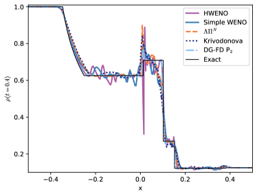
(a) Riemann Problem 1 comparison

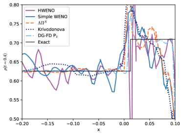
(b) Zoom in of Riemann Problem 1

Figure 1: A comparison of different limiters used to stabilize the evolution of the Riemann Problem 1 of [66]. The problem is solved using 128 third-order (P₂) elements. The DG-FD hybrid scheme significantly outperforms the other limiters both in robustness and accuracy.

While all five limiting strategies evolve to the final time, the DG-FD scheme is the least oscillatory and is also able to resolve the discontinuities much more accurately. The HWENO scheme is slightly less oscillatory if linear neighbor weights of $\gamma_{k}=0.01$ are used instead of $\gamma_{k}=0.001$. However, the simple WENO limiter fails to evolve the solution with $\gamma_{k}=0.01$ and such sensitivity to parameters in the algorithm is not desirable when solving realistic problems. Going to higher order has proven to be especially challenging. While both the $\Lambda\Pi^{N}$ and the Krivodonova complete the evolution when using a P₅ scheme with 64 elements (simple WENO and HWENO fail), additional spurious oscillations are present. In comparison, the DG-FD hybrid scheme actually has fewer oscillations when going to higher order. In Fig. 2 we plot the error of the numerical solution using a P₂ DG-FD scheme with 128 elements and a P₅ DG-FD scheme with 64 elements. We see that the P₅ hybrid scheme actually has fewer oscillations than the P₂ scheme, while resolving the discontinuities equally well. We attribute this to the troubled-cell indicators actually triggering earlier when a higher polynomial degree is used since discontinuities entering an element rapidly dump energy into the high modes. While we will compare the different limiting strategies for 2d and 3d problems below, it is already quite apparent that the DG-FD hybrid scheme is by far the most robust and accurate method.

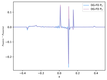
Figure 2: The difference between the analytic and numerical solution of the Riemann Problem 1 of [66] at $t=0.4$ for the DG-FD P₂ scheme (solid light blue curve) and the DG-FD P₅ scheme (dashed purple curve). The P₅ scheme is able to resolve the discontinuities just as well as the P₂ scheme, while also admitting fewer unphysical oscillations away from the discontinuities.

IV.3 2d cylindrical blast wave

A standard test problem for GRMHD codes is the cylindrical blast wave [68, 69], where a magnetized fluid initially at rest in a constant magnetic field along the $x$-axis is evolved. The fluid obeys the ideal fluid equation of state (63) with $\gamma=4/3$. The fluid begins in a cylindrically symmetric configuration, with hot, dense fluid in the region with cylindrical radius $r<0.8$ surrounded by a cooler, less dense fluid in the region $r>1$. The initial density $\rho$ and pressure $p$ of the fluid are

$$\begin{split}\rho(r<0.8)&=10^{-2},\\ \rho(r>1.0)&=10^{-4},\\ p(r<0.8)&=1,\\ p(r>1.0)&=5\times 10^{-4}.\end{split}$$ (66)

In the region $0.8\leq r\leq 1$, the solution transitions continuously and exponentially (i.e., transitions such that the logarithms of the pressure and density are linear functions of $r$). The fluid begins threaded with a uniform magnetic field with Cartesian components

$$(B^{x},B^{y},B^{z})=(0.1,0,0).$$ (67)

The magnetic field causes the blast wave to expand non-axisymmetrically. For all simulations we use a time step size $\Delta t=10^{-2}$ and an SSP RK3 time integrator.

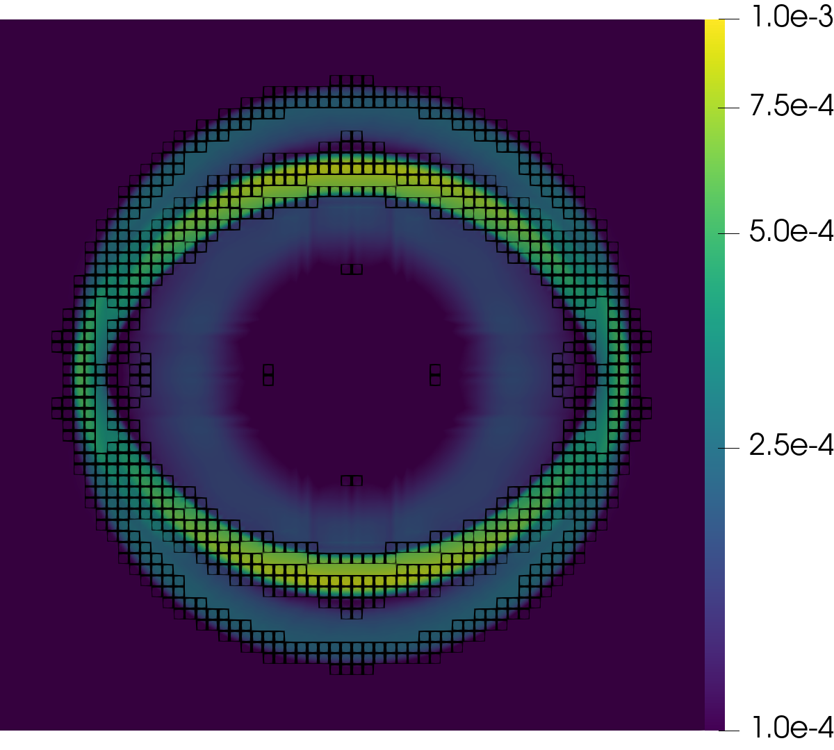
(a) DG-FD, P₂, $64^{2}$ elements

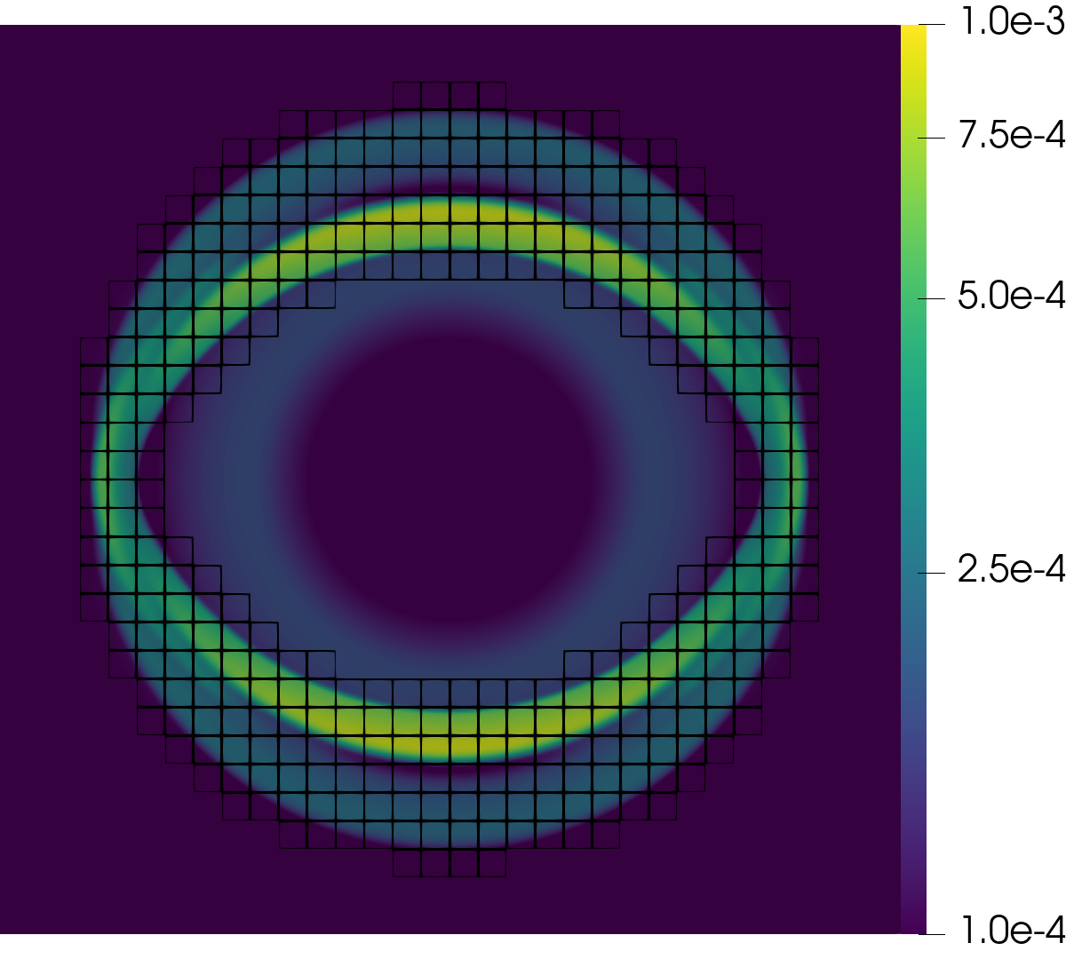
(b) DG-FD, P₅, $32^{2}$ elements

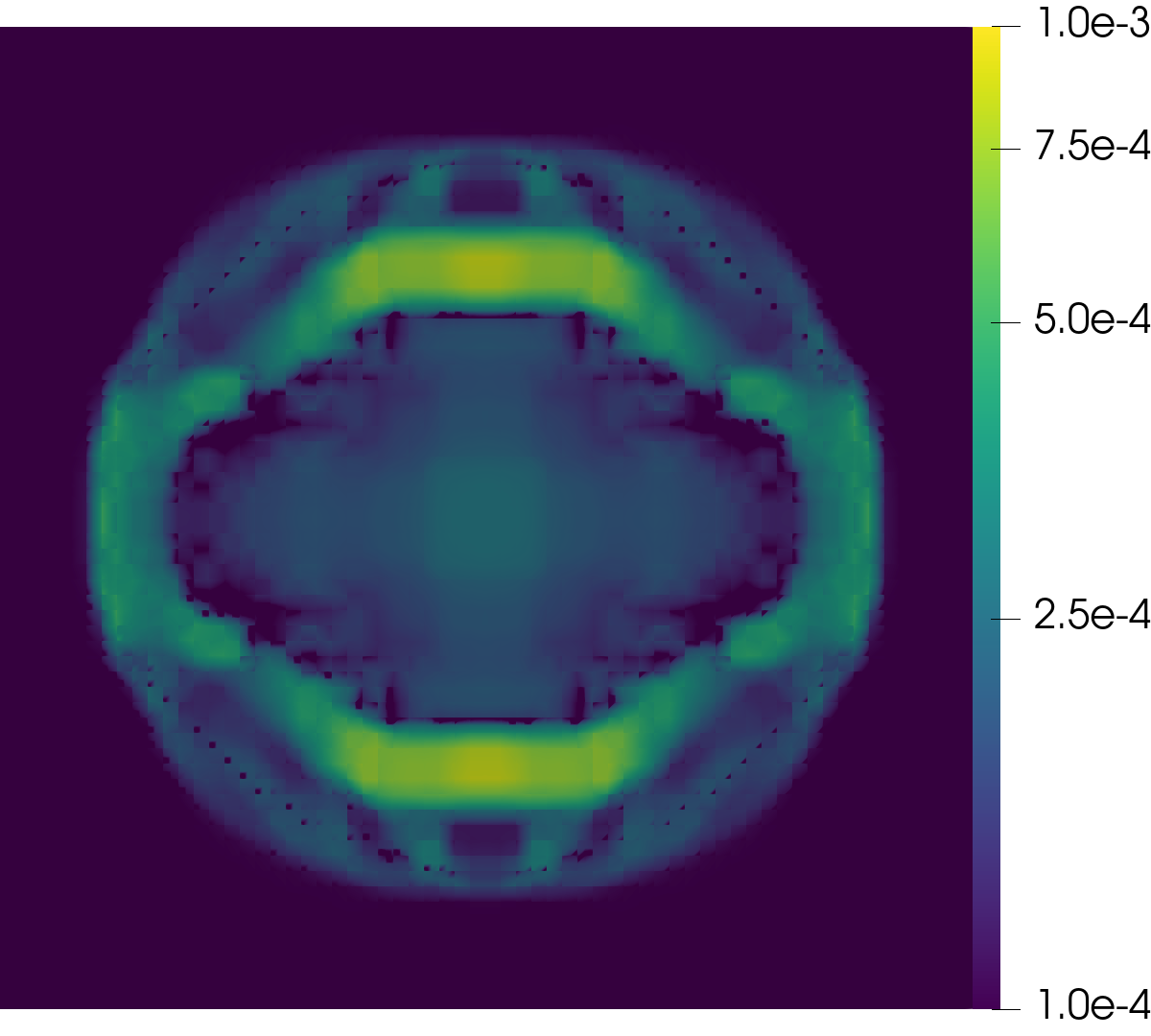
(c) $\Lambda\Pi^{N}$, P₂, $64^{2}$ elements

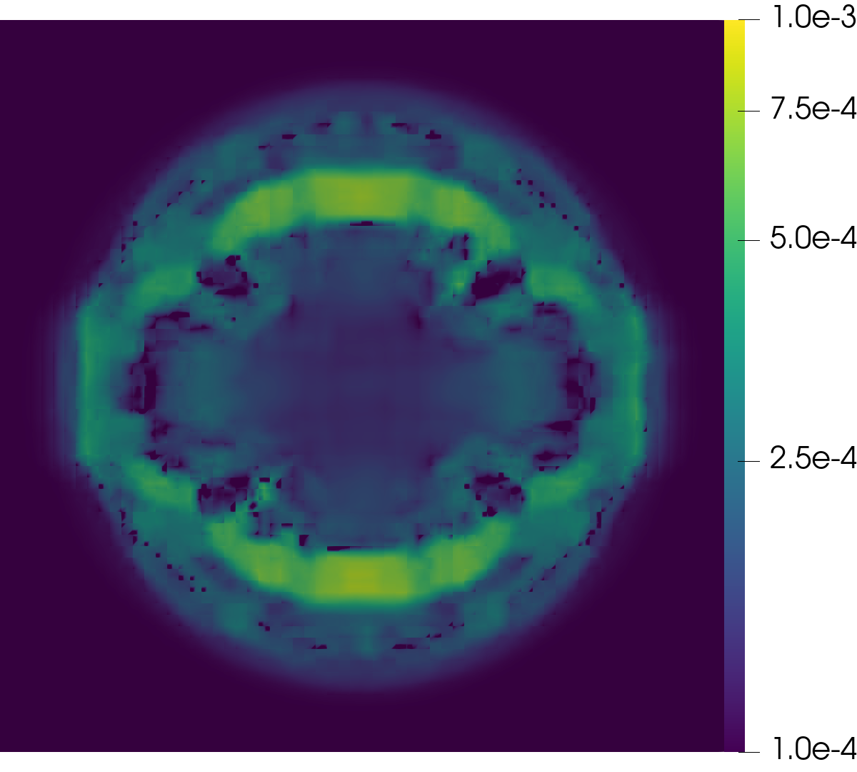
(d) Krivodonova, P₂, $64^{2}$ elements

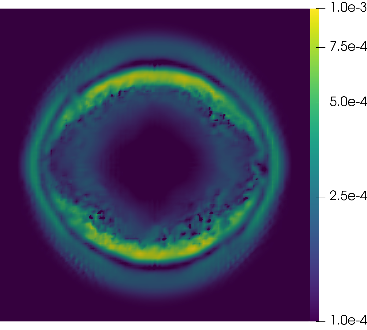
(e) Simple WENO, P₂, $64^{2}$ elements

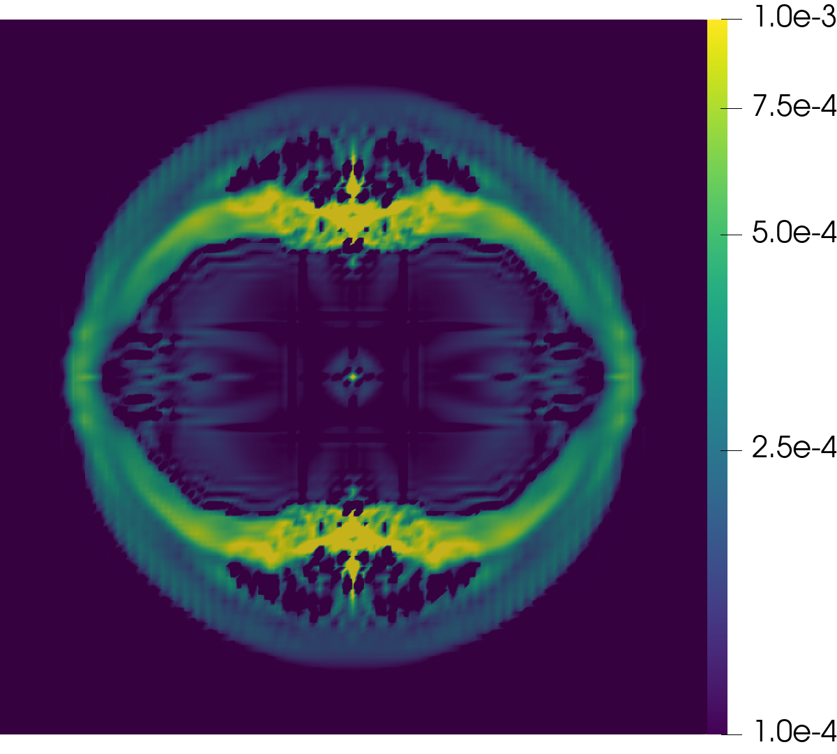
(f) HWENO, P₂, $64^{2}$ elements

Figure 3: Cylindrical blast wave $\rho$ at $t=4$ comparing the DG-FD hybrid scheme, the $\Lambda\Pi^{N}$, Krivodonova, simple WENO, and HWENO limiters using P₂ DG, as well as the DG-FD scheme using P₅ DG. There are 192 degrees of freedom per dimension, comparable to what is used when testing FD schemes. We see that only the DG-FD hybrid scheme really resolves the features to an acceptable level, and the $\Lambda\Pi^{N}$ and Krivodonova smear out the solution almost completely. In the plots of the DG-FD hybrid scheme the regions surrounded by black squares have switched from DG to FD at the final time.

We evolve the blast wave to time $t=4.0$ on a grid of $64\times 64\times 1$ elements covering a cube of extent $[-6,6]^{3}$ using a DG P₂ scheme, a comparable resolution to what FD code tests use. We apply periodic boundary conditions in all directions, since the explosion does not reach the outer boundary by $t=4.0$. Figure 3 shows the logarithm of the rest-mass density at time $t=4.0$, at the end of evolutions using the different limiting strategies. We see from Fig. 3c and Fig. 3d that the $\Lambda\Pi^{N}$ and Krivodonova limiters result in a very poorly resolved solution. The simple WENO evolution, Fig. 3e is much better but still not nearly as good as a FD method with the same number of degrees of freedom. The HWENO limiter, Fig. 3f, suffers from various spurious artifacts. The DG-FD hybrid scheme, however, again demonstrates its ability to robustly handle discontinuities, while also resolving smooth features with very high order. Figure 3a shows the result of a simulation using a P₂ DG-FD scheme and Fig. 3b using a P₅ DG-FD scheme with half the number of elements. The increased resolution of a high-order scheme is clear when comparing the P₂ and P₅ solutions in the interior region of the blast wave. We conclude that the DG-FD hybrid scheme is the most robust and accurate method/limiting strategy for solving the cylindrical blast wave problem.

IV.4 2d magnetic rotor

The second 2-dimensional test problem we study is the magnetic rotor problem originally proposed for non-relativistic MHD [70, 71] and later generalized to the relativistic case [72, 73]. A rapidly rotating dense fluid cylinder is inside a lower density fluid, with a uniform pressure and magnetic field everywhere. The magnetic braking will slow down the rotor over time, with an approximately 90 degree rotation by the final time $t=0.4$. We use a domain of $[-0.5,0.5]^{3}$ and a time step size $\Delta t=10^{-3}$ and an SSP RK3 time integrator. An ideal fluid equation of state with $\Gamma=5/3$ is used, and the following initial conditions are imposed:

$$\begin{split}p&=1\\ B^{i}&=(1,0,0)\\ v^{i}&=\left\{\begin{array}[]{ll}(-y\Omega,x\Omega,0),&\mathrm{if}\;r\leq R_{\mathrm{rotor}}=0.1\\ (0,0,0),&\mathrm{otherwise},\end{array}\right.\\ \rho&=\left\{\begin{array}[]{ll}10,&\mathrm{if}\;r\leq R_{\mathrm{rotor}}=0.1\\ 1,&\mathrm{otherwise},\end{array}\right.\end{split}$$ (68)

with angular velocity $\Omega=9.95$. The choice of $\Omega$ and $R_{\mathrm{rotor}}=0.1$ guarantees that the maximum velocity of the fluid (0.995) is less than the speed of light.

(a) DG-FD, P₂, $64^{2}$ elements

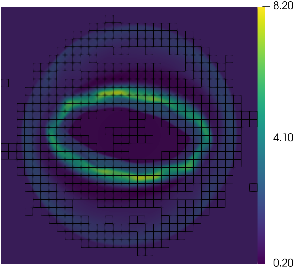
(b) DG-FD, P₅, $32^{2}$ elements

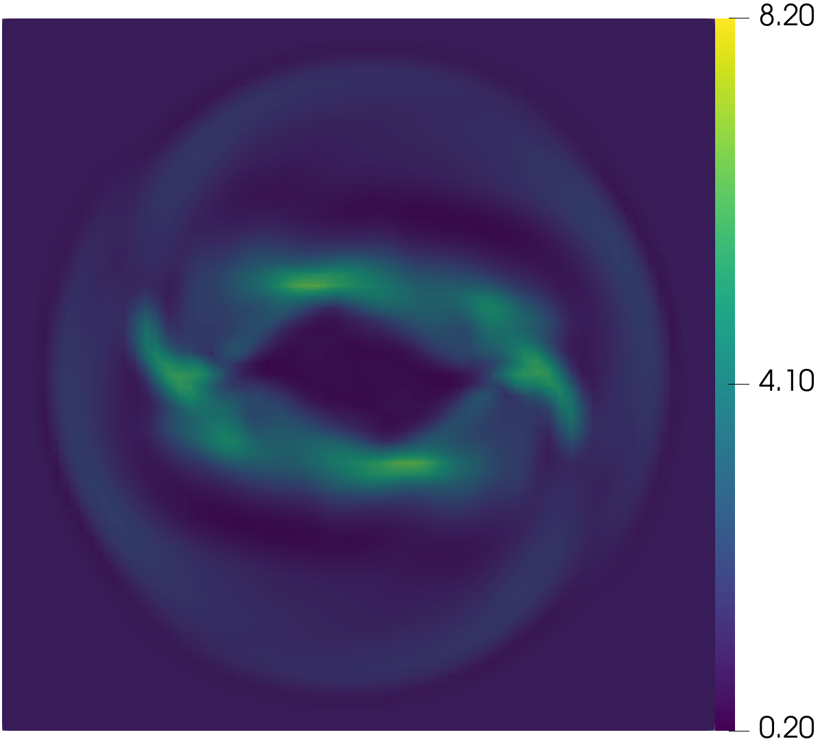
(c) $\Lambda\Pi^{N}$, P₂, $64^{2}$ elements

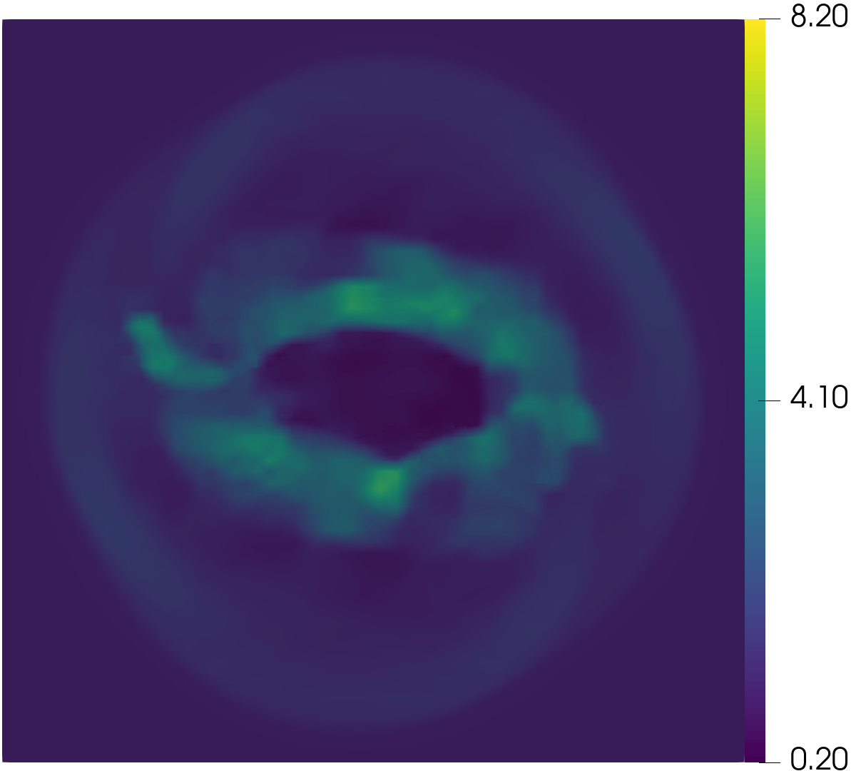
(d) Krivodonova, P₂, $64^{2}$ elements

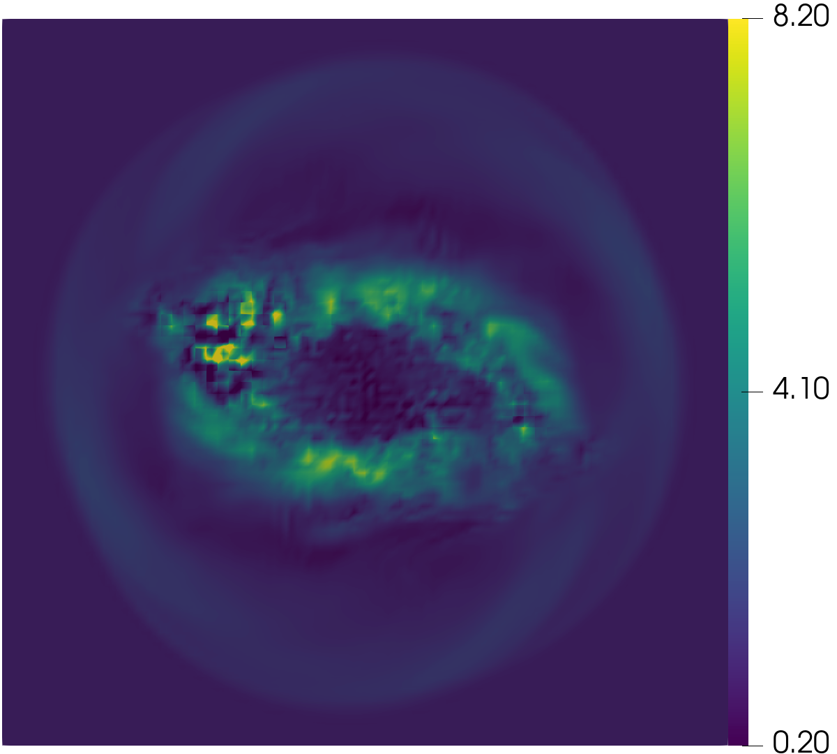
(e) Simple WENO, P₂, $64^{2}$ elements

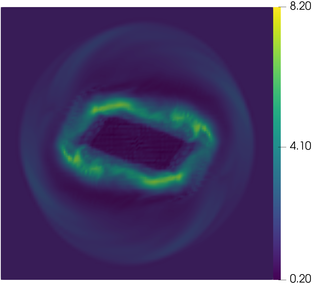
(f) HWENO, P₂, $64^{2}$ elements

Figure 4: Magnetic rotor $\rho$ at $t=0.4$ comparing the DG-FD hybrid scheme, the $\Lambda\Pi^{N}$, Krivodonova, simple WENO, and HWENO limiters using P₂ DG, as well as the DG-FD scheme using P₅ DG. There are 192 degrees of freedom per dimension, comparable to what is used when testing FD schemes. We see that only the DG-FD hybrid scheme really resolves the features to an acceptable level, and the $\Lambda\Pi^{N}$ and Krivodonova smear out the solution almost completely. The simple WENO limiter fails to solve the problem. In the plots of the DG-FD hybrid scheme the regions surrounded by black squares have switched from DG to FD at the final time.

We show the results of our evolutions in Fig. 4, which are all done with 192 grid points and periodic boundary conditions. Figures 4c and 4d show results using the $\Lambda\Pi^{N}$ and Krivodonova limiter which both severely smear out the solution. The simple WENO limiter suffers from spurious artifacts (Fig. 4e), while the HWENO limiter does a reasonable job (Fig. 4f). The DG-FD hybrid scheme is most robust and accurate, but a fairly large number of cells end up being marked as troubled in this problem and switched to FD. While ideally fewer cells would be switched to FD, it is better to have a scheme that is capable of solving a large array of problems without fine-tuning than to have a slightly different fine-tuned scheme for each test problem.

IV.5 2d magnetic loop advection

The third 2-dimensional test problem we study is magnetic loop advection problem [74]. A magnetic loop is advected through the domain until it returns to its starting position. We use an initial configuration very similar to [42, 75, 76, 77], where

$$\begin{split}\rho&=1\\ p&=3\\ v^{i}&=(1/1.2,1/2.4,0)\\ B^{x}&=\left\{\begin{array}[]{ll}-A_{\mathrm{loop}}y/R_{\mathrm{in}},&\mathrm{if}\;r\leq R_{\mathrm{in}}\\ -A_{\mathrm{loop}}y/r,&\mathrm{if}\;R_{\mathrm{in}}<r<R_{\mathrm{loop}}\\ 0,&\mathrm{otherwise},\end{array}\right.\\ B^{y}&=\left\{\begin{array}[]{ll}A_{\mathrm{loop}}x/R_{\mathrm{in}},&\mathrm{if}\;r\leq R_{\mathrm{in}}\\ A_{\mathrm{loop}}x/r,&\mathrm{if}\;R_{\mathrm{in}}<r<R_{\mathrm{loop}}\\ 0,&\mathrm{otherwise},\end{array}\right.\end{split}$$ (69)

with $R_{\mathrm{loop}}=0.3$, $R_{\mathrm{in}}=0.001$, and an ideal gas equation of state with $\Gamma=5/3$. The computational domain is $[-0.5,0.5]^{3}$ with $64\times 64\times 1$ elements and periodic boundary conditions being applied everywhere. The final time for one period is $t=2.4$. For all simulations we use a time step size $\Delta t=10^{-3}$ and an SSP RK3 time integrator.

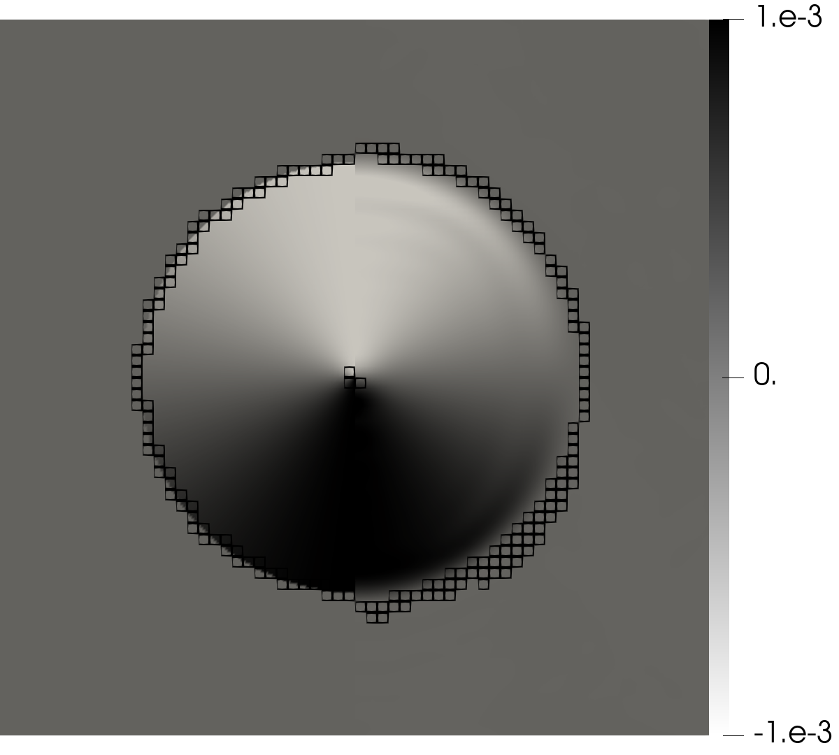
(a) DG-FD, P₂, $64^{2}$ elements

(b) DG-FD, P₅, $32^{2}$ elements

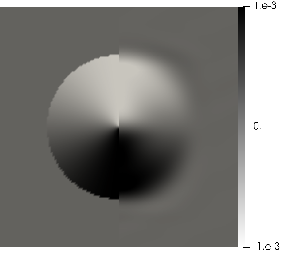
(c) $\Lambda\Pi^{N}$, P₂, $64^{2}$ elements

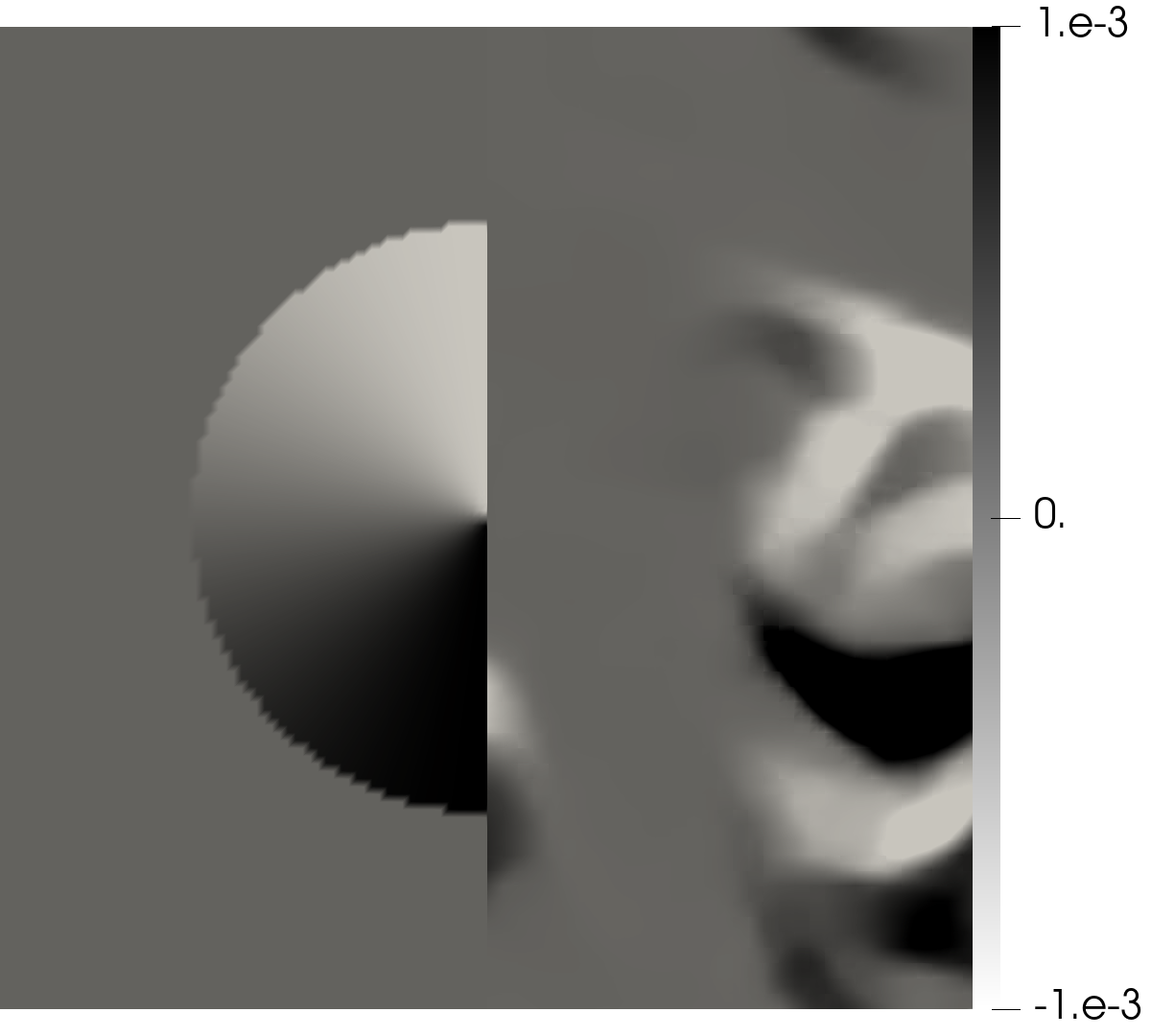
(d) Krivodonova, P₂, $64^{2}$ elements

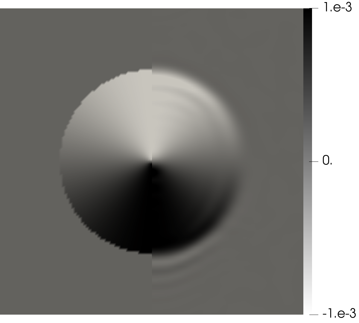
(e) Simple WENO, P₂, $64^{2}$ elements

(f) HWENO, P₂, $64^{2}$ elements

Figure 5: $B^{x}$ for the magnetic loop advection problem. The left half of each plot is at the initial time, while the right half is after one period ($t=2.4$). We compare the DG-FD hybrid scheme, the $\Lambda\Pi^{N}$, Krivodonova, simple WENO, and HWENO limiters using P₂ DG, as well as the DG-FD scheme using P₅ DG. There are 192 degrees of freedom per dimension, comparable to what is used when testing FD schemes. In the plots of the DG-FD hybrid scheme the regions surrounded by black squares have switched from DG to FD at the final time.

In Fig. 5 we plot the magnetic field component $B^{x}$ at $t=0$ on the left half of each plot and after one period $t=2.4$ on the right half of each plot for results using various limiting strategies. We use a TVB constant of 5 for the $\Lambda\Pi^{N}$, simple WENO, and HWENO limiters, and use neighbor weights $\gamma_{k}=0.001$ for the simple WENO and HWENO limiters. The Krivodonova limiter completely destroys the solution and only remains stable because of our conservative variable fixing scheme. Both WENO limiters work quite well, maintaining the shape of the loop with only some oscillations being generated. The DG-FD hybrid scheme again performs the best. In Fig. 5a we show the result using a P₂ DG-FD scheme and in Fig. 5b using a P₅ DG-FD scheme. The P₅ scheme resolves the smooth parts of the solution more accurately than the P₂ scheme, as is to be expected. The DG-FD hybrid scheme also does not generate the spurious oscillations that are present when using the WENO limiters. While the spurious oscillations may be reduced by fine-tuning the TVB constant and the neighbor weights, this type of fine-tuning is not possible for complex physics simulations and so we do not spend time searching for the “optimal” parameters.

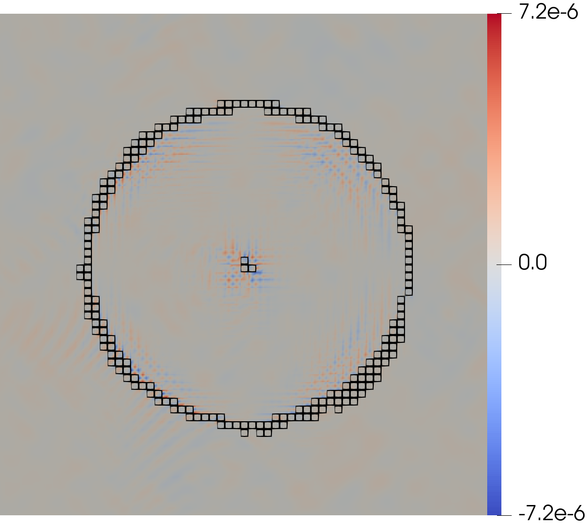
(a) DG-FD, P₂, $64^{2}$ elements

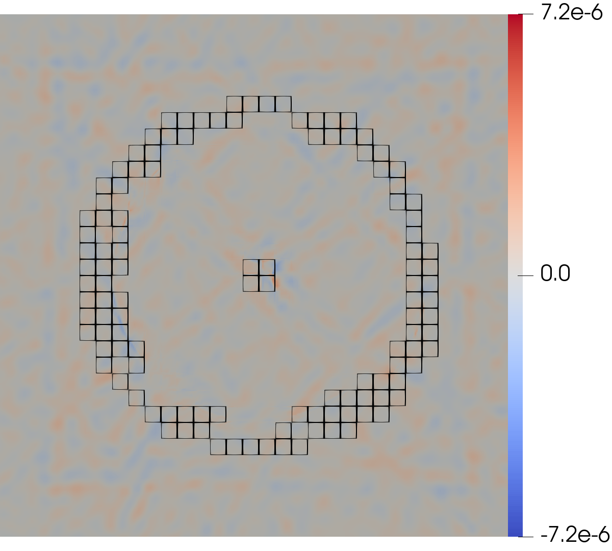
(b) DG-FD, P₅, $32^{2}$ elements

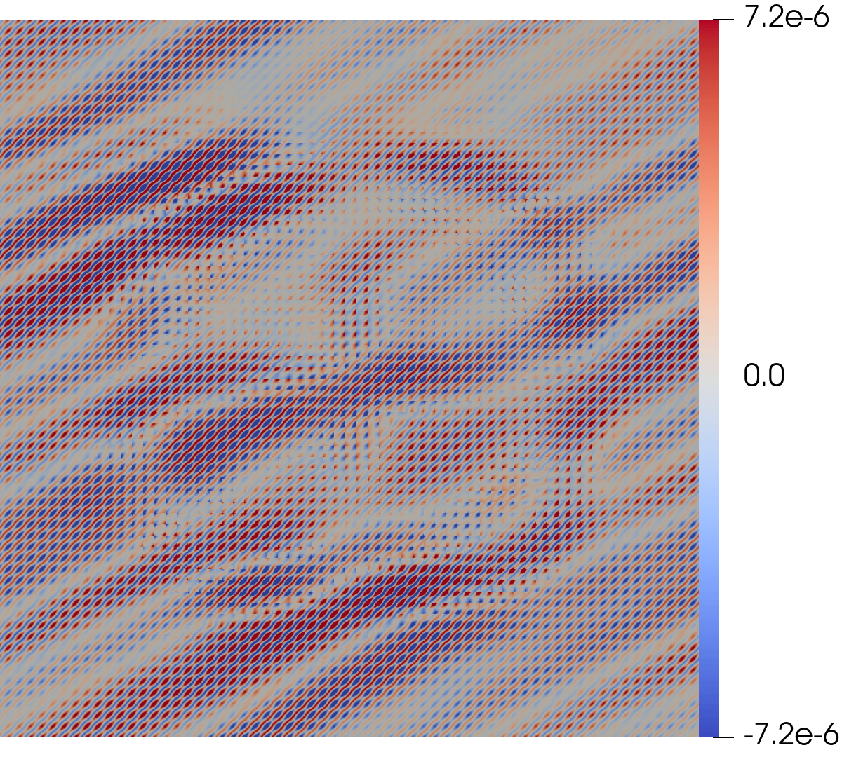
(c) $\Lambda\Pi^{N}$, P₂, $64^{2}$ elements

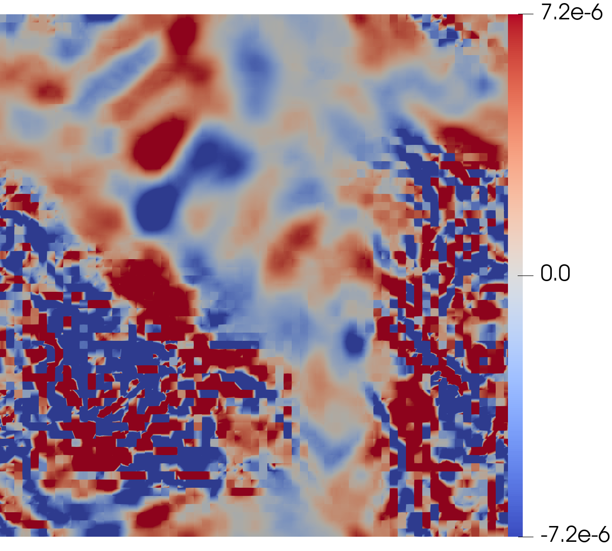
(d) Krivodonova, P₂, $64^{2}$ elements

(e) Simple WENO, P₂, $64^{2}$ elements

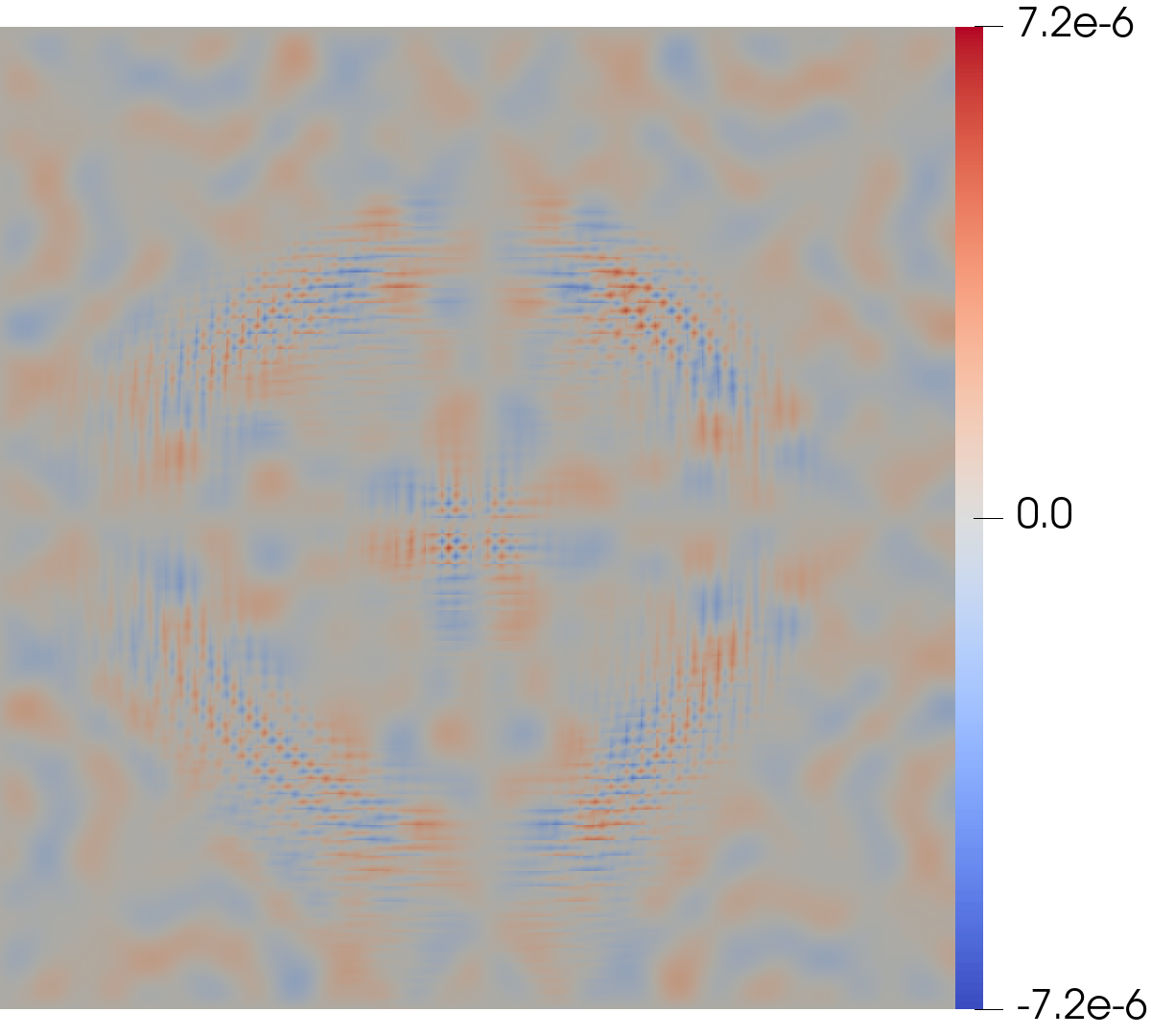
(f) HWENO, P₂, $64^{2}$ elements

Figure 6: The divergence cleaning field $\Phi$ for the magnetic loop advection problem after one period ($t=2.4$) comparing the DG-FD hybrid scheme, the $\Lambda\Pi^{N}$, Krivodonova, simple WENO, and HWENO limiters using P₂ DG, as well as the DG-FD scheme using P₅ DG. There are 192 degrees of freedom per dimension, comparable to what is used when testing FD schemes. In the plots from the DG-FD hybrid scheme the regions surrounded by black squares have switched from DG to FD at the final time.

Since we are using hyperbolic divergence cleaning, violations of the $\partial_{i}B^{i}=0$ constraint occur. In Fig. 6 we plot the divergence cleaning field $\Phi$ at the final time $t=2.4$. The simple WENO, HWENO, and DG-FD hybrid schemes all have $|\Phi|\sim 5\times 10^{-6}$, while the $\Lambda\Pi^{N}$ limiter has $\Phi$ approximately one order of magnitude larger. For the magnetic loop advection problem we find that all classical limiters perform comparably, except the Krivodonova limiter completely destroys the solution and remains stable only because of our conservative variable fixing scheme. Nevertheless, the DG-FD hybrid scheme is better than the classical limiters, and we conclude that the DG-FD hybrid scheme is both the most robust and accurate method/limiting strategy for solving the magnetic loop advection problem.

IV.6 2d magnetized Kelvin-Helmholtz instability

The last 2-dimensional test problem we study is the magnetized Kelvin-Helmholtz (KH) instability, similar to [78]. The domain is $[0,1]^{3}$ and we use the following initial conditions [18]:

$$\rho =\begin{cases}1,&\left|y-0.5\right|<0.25\\ 10^{-2},&\text{otherwise},\end{cases}$$ (70)

$$p =1.0,$$ (71)

$$v^{x} =\begin{cases}0.5,&\left|y-0.5\right|<0.25\\ -0.5,&\text{otherwise},\end{cases}$$ (72)

$$v^{y} =0.1\sin(4\pi x)\left[\exp\left(-\dfrac{(y-0.75)^{2}}{0.0707^{2}}\right)\right.$$

$$\left.+\exp\left(-\dfrac{(y-0.25)^{2}}{0.0707^{2}}\right)\right],$$ (73)

$$v^{z} =0.0,$$ (74)

$$B^{x} =10^{-3},$$ (75)

$$B^{y} =B^{z}=0.0.$$ (76)

We use an ideal gas equation of state with $\Gamma=4/3$, a final time $t_{f}=1.6$, a time step size of $\Delta t=10^{-3}$, an SSP RK3 time integrator, and $[64\times 1\times 64]$ P₂ elements for the classical limiters. For the DG-FD hybrid method we use both $[64\times 1\times 64]$ P₂ elements and $[32\times 1\times 32]$ P₅ elements. We use a TVB constant of $1$ for all the limiters. Using the flattening algorithm is crucial for the results obtained here, while for other test problems it is significantly less important.

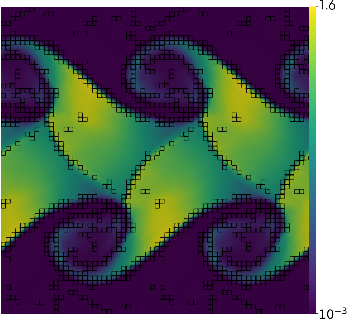
(a) DG-FD, P₂, $64^{2}$ elements

(b) DG-FD, P₅, $32^{2}$ elements

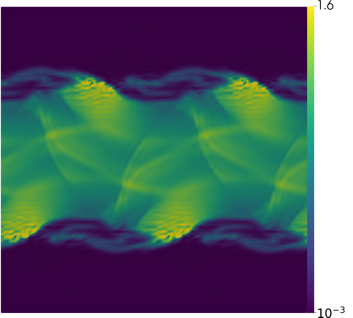
(c) $\Lambda\Pi^{N}$, P₂, $64^{2}$ elements

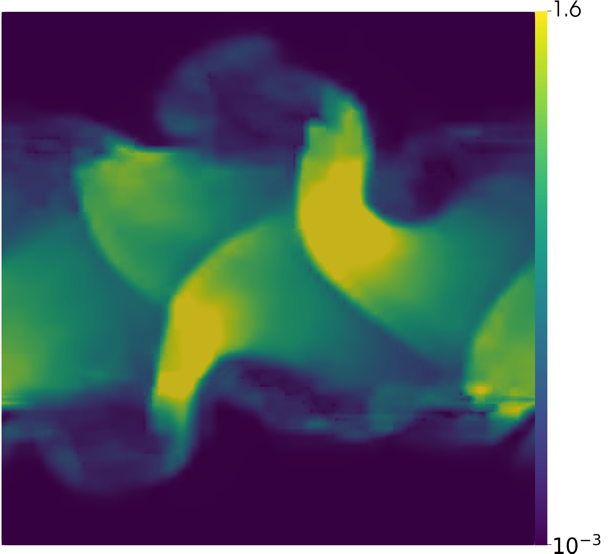
(d) Krivodonova, P₂, $64^{2}$ elements

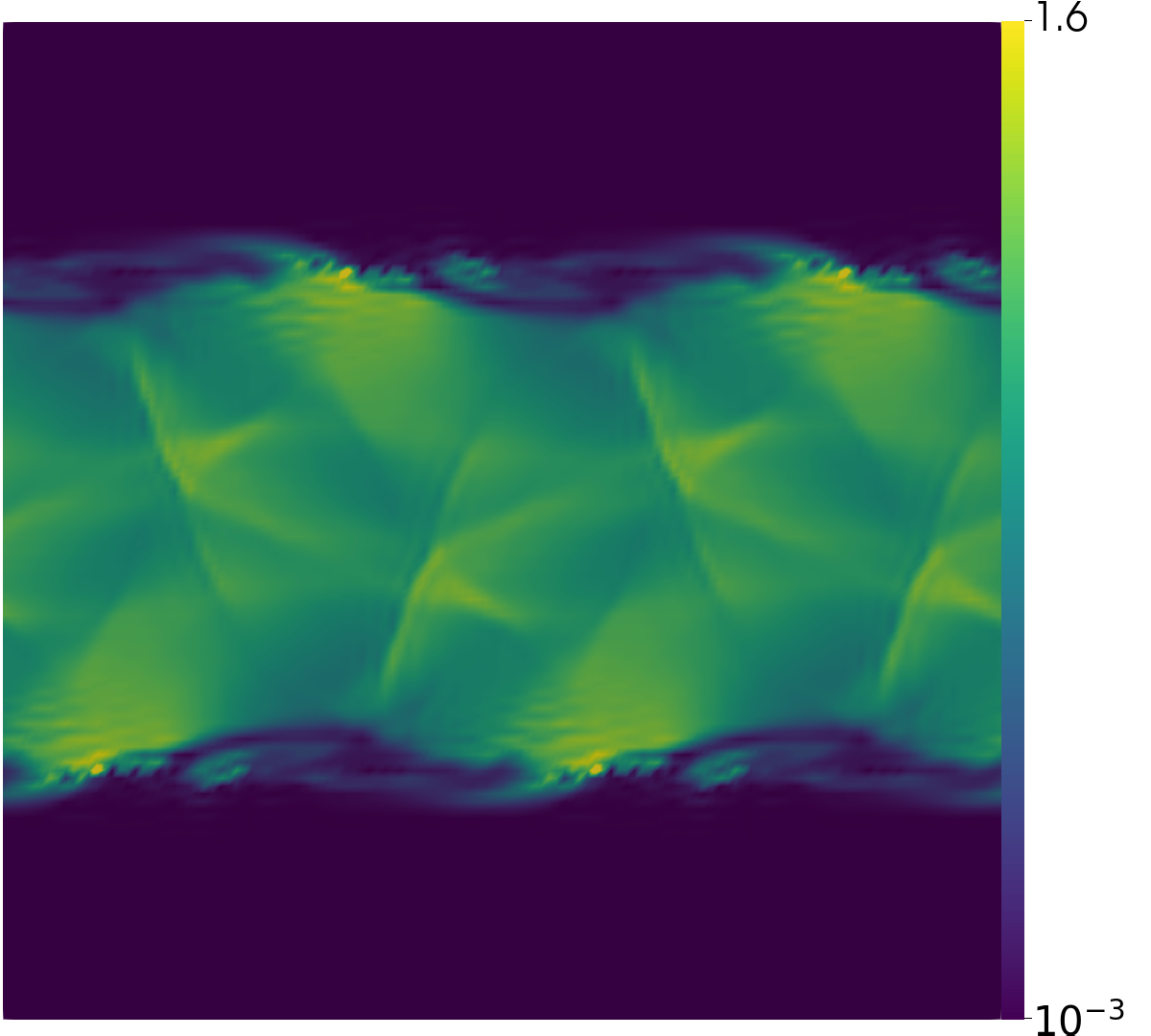
(e) Simple WENO, P₂, $64^{2}$ elements

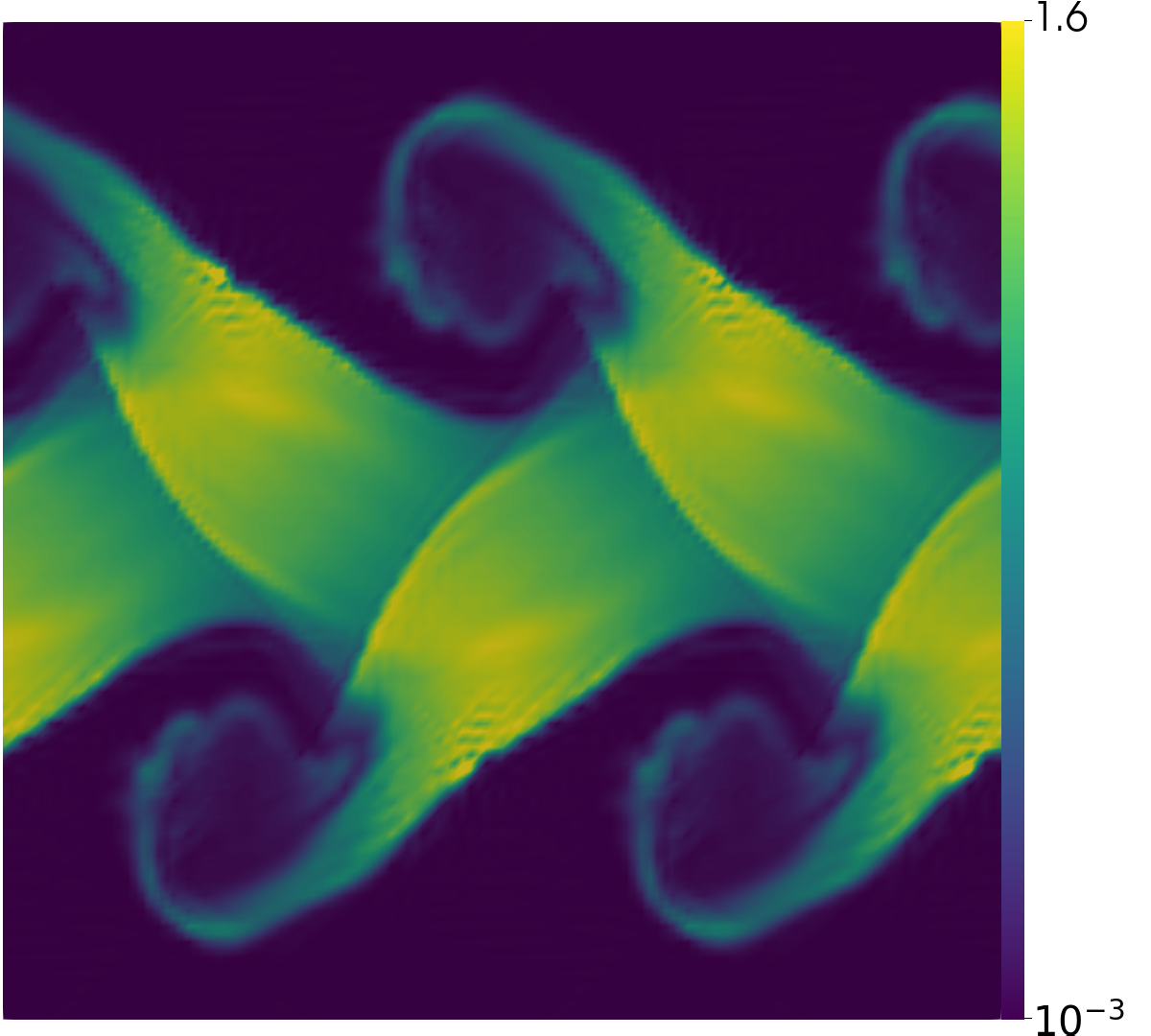
(f) HWENO, P₂, $64^{2}$ elements

Figure 7: Magnetized Kelvin-Helmholtz instability $\rho$ at $t=1.6$ comparing the DG-FD hybrid scheme, the $\Lambda\Pi^{N}$, Krivodonova, simple WENO, and HWENO limiters using P₂ DG, as well as the DG-FD scheme using P₅ DG. There are 192 degrees of freedom per dimension, comparable to what is used when testing FD schemes. Only the DG-FD hybrid scheme and the HWENO limiter produce reasonable results, while the $\Lambda\Pi^{N}$ limiter has very low effective resolution, and the Krivodonova and Simple WENO limiters smear out the solution almost completely. In the plots of the DG-FD hybrid scheme the regions surrounded by black squares have switched from DG to FD at the final time.

In Fig. 7 we plot the density at the final time comparing the different limiting strategies. From Fig. 7e and 7d we see that the Simple WENO and Krivodonova limiters destroy the solution almost completely. The $\Lambda\Pi^{N}$ limiter (Fig. 7c) retains some hints of the expected flow pattern, but also nearly completely destroys the solution. The HWENO limiter is plotted in Fig. 7f and does by far the best of the classical limiters. Ultimately, only the DG-FD hybrid method (Fig. 7a for P₂ and Fig. 7b for P₅) is able to produce the expected vortices and flow patterns.

IV.7 TOV star

A rigorous 3d test case in general relativity is the evolution of a static, spherically symmetric star. The Tolman-Oppenheimer-Volkoff (TOV) solution [79, 80] describes such a setup. In this section we study evolutions of both non-magnetized and magnetized TOV stars. We adopt the same configuration as in [81]. Specifically, we use a polytropic equation of state,

$$p(\rho)=K\rho^{\Gamma}$$ (77)

with the polytropic exponent $\Gamma=2$, polytropic constant $K=100$, and a central density $\rho_{c}=1.28\times 10^{-3}$. When considering a magnetized star we choose a magnetic field given by the vector potential

$$A_{\phi}=A_{b}(x^{2}+y^{2})\max(p-p_{\mathrm{cut}},0)^{n_{s}},$$ (78)

with $A_{b}=2500$, $p_{\mathrm{cut}}=0.04p_{\max}$, and $n_{s}=2$. This configuration yields a magnetic field strength in CGS units

$$|B_{\mathrm{CGS}}|=\sqrt{b^{2}}\times 8.352\times 10^{19}\,\mathrm{G},$$ (79)

of $|B_{\mathrm{CGS}}|=1.03\times 10^{16}\,G$. The magnetic field is only a perturbation to the dynamics of the star, since $(p_{\text{mag}}/p)(r=0)\sim 5\times 10^{-5}$. However, evolving the field stably and accurately can be challenging. The magnetic field corresponding to the vector potential in Eq. (78) in the magnetized region is given by

$$\begin{split}B^{x}&=\frac{1}{\sqrt{\gamma}}\frac{xz}{r}A_{b}n_{s}(p-p_{\mathrm{cut}})^{n_{s}-1}\partial_{r}p,\\ B^{y}&=\frac{1}{\sqrt{\gamma}}\frac{yz}{r}A_{b}n_{s}(p-p_{\mathrm{cut}})^{n_{s}-1}\partial_{r}p,\\ B^{z}&=-\frac{A_{b}}{\sqrt{\gamma}}\left[2(p-p_{\mathrm{cut}})^{n_{s}}\phantom{\frac{a}{b}}\right.\\ &\left.+\frac{x^{2}+y^{2}}{r}n_{s}(p-p_{\mathrm{cut}})^{n_{s}-1}\partial_{r}p\right],\end{split}$$ (80)

and at $r=0$ is

$$\begin{split}B^{x}&=0,\\ B^{y}&=0,\\ B^{z}&=-\frac{A_{b}}{\sqrt{\gamma}}2(p-p_{\mathrm{cut}})^{n_{s}}.\end{split}$$ (81)

We perform all evolutions in full 3d with no symmetry assumptions and in the Cowling approximation, i.e., we do not evolve the spacetime. To match the resolution usually used in FD/FV numerical relativity codes we use a domain $[-20,20]^{3}$ with a base resolution of 6 P₅ DG elements and 12 P₂ DG elements. This choice means we have approximately 32 FD grid points covering the star’s diameter at the lowest resolution, 64 when using 12 P₅ elements, and 128 grid points when using 24 P₅ elements. In all cases we set $\rho_{\mathrm{atm}}=10^{-15}$ and $\rho_{\mathrm{cutoff}}=1.01\times 10^{-15}$.

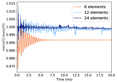
Figure 8: The maximum density over the grid $\max(\rho)$ divided by the maximum density over the grid at $t=0$ for three different resolution for the non-magnetized TOV star simulations. The 6-element simulation uses FD throughout the interior of the star, while 12- and 24-element simulations use DG. The increased high-frequency content in 12- and 24-element simulations occurs because the high-order DG scheme is able to resolve higher oscillation modes in the star. The maximum density in the 6-element case drifts down at early times because of the low resolution and the relatively low accuracy of using FD at the center.

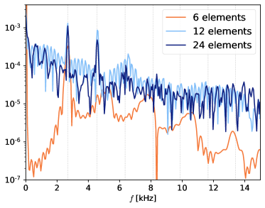
Figure 9: The power spectrum of the maximum density for three different resolutions for the non-magnetized TOV star simulations. The 6-element simulation uses FD throughout the interior of the star, while the 12- and 24-element simulations use DG. When the high-order DG scheme is used, more oscillation frequencies are resolved. The vertical dashed lines correspond to the known frequencies in the Cowling approximation [82].

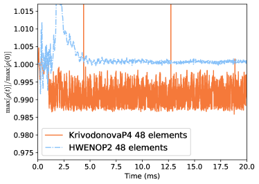
Figure 10: The maximum density over the grid $\max(\rho)$ divided by the maximum density over the grid at $t=0$ for the best two cases using classical limiters for the non-magnetized TOV star simulations. The HWENO limiter is only stable for a P₂ DG solver. Simple WENO (not plotted) gives similar results. The Krivodonova limiter only succeeded at some resolutions (3 of the 16 attempted runs) and the shown best result is noticeably noisier than the subcell limiter.

In Fig. 8 we show the normalized maximum rest mass density over the grid for the non-magnetized TOV star. The 6-element simulation uses FD throughout the interior of the star and so there is no grid point at $r=0$. This is the reason the data is shifted compared to 12- and 24-element simulations, where the unlimited P₅ DG solver is used throughout the star interior and so there is a grid point at the center of the star. The increased “noise” in the 12- and 24-element data actually stems from the higher oscillation modes in the star that are induced by numerical error. In Fig. 9 we plot the power spectrum using data at the three different resolutions. The 6-element simulation only has one mode resolved, while 12 elements resolve two modes well, and the 24-element simulation resolves three modes well. In Fig. 10 we show the normalized maximum rest mass density over the grid for the best two cases using the classical limiters. The simple WENO and HWENO limiters performed similarly and were only stable for P₂. The Krivodonova limiter only succeeded at 3 of the 16 resolutions we attempted, and its best result is noticeably noisier than the other limiters. Note that our experience is consistent with that of reference [21], which was unable to achieve stable evolutions of a 3d TOV star using the simple WENO limiter.

We show the normalized maximum rest mass density over the grid for the magnetized TOV star in Fig. 11. Overall the results are nearly identical to the non-magnetized case. One notable difference is the decrease in the 12-element simulation between 7.5ms and 11ms, which occurs because the code switches from DG to FD at the center of the star at 7.5ms and back to DG at 11ms. Nevertheless, the frequencies are resolved just as well for the magnetized star as for the non-magnetized case, as can be seen in Fig. 12 where we plot the power spectrum. Specifically, we are able to resolve the three largest modes with our P₅ DG-FD hybrid scheme. To the best of our knowledge, these are the first simulations of a magnetized neutron star using high-order DG methods.

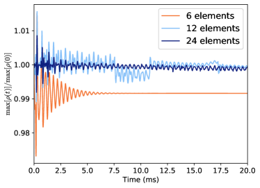
Figure 11: The maximum density over the grid $\max(\rho)$ divided by the maximum density over the grid at $t=0$ for three different resolution for the magnetized TOV star simulation. The 6-element simulation uses FD throughout the interior of the star, while 12- and 24-element simulations use DG. The increased high-frequency content in 12- and 24-element simulations occurs because the high-order DG scheme is able to resolve higher oscillation modes in the star. The maximum density in the 6-element case drifts down at early times because of the low resolution and the relatively low accuracy of using FD at the center.

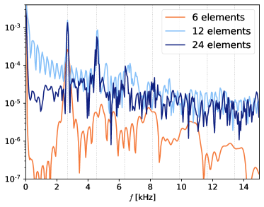
Figure 12: The power spectrum of the maximum density for three different resolutions of the magnetized TOV star simulations. The 6-element simulation uses FD throughout the interior of the star, while the 12- and 24-element simulations use DG. When the high-order DG scheme is used, more oscillation frequencies are resolved. The vertical dashed lines correspond to the known frequencies in the Cowling approximation.

V Conclusions

We compare various shock capturing strategies to stabilize the DG method applied to the equations of general relativistic magnetohydrodynamics in the presence of discontinuities and shocks. We use the open source numerical relativity code SpECTRE [35] to perform the simulations. We compare the classic $\Lambda\Pi^{N}$ method [29], the hierarchical limiter of Krivodonova [30], the simple WENO limiter [31], the HWENO limiter [32], and a DG-FD hybrid approach that uses DG where the solution is smooth and HRSC FD methods where the solution contains discontinuities[56]. While many of the limiting strategies appear promising in the Newtonion hydrodynamics case, we have found stable and accurate simulations of GRMHD to be a much more challenging problem. This is in part because limiting the characteristic variables is difficult since the characteristic variables are not known analytically for the GRMHD system.

In the Newtonian hydrodynamics case, the literature advocates for using the classical limiters ($\Lambda\Pi^{N}$, Krivodonova, simple WENO, HWENO) on the characteristic variables of the evolution system to reduce oscillations, for using more detailed troubled-cell indicators like that of [55], and for supplementing the limiting with flattening schemes to further correct any unphysical values remaining after limiting. We have found these techniques do somewhat improve the accuracy and robustness of the limiters in the Newtonian case, but not enough to avoid the need for problem-dependent tuning of parameters, or to obtain truly robust behavior. Since these techniques do not all easily generalize to the relativistic magnetohydrodynamics case we consider here, we use the classical limiters in their simplest configuration. Our experience with limiters in Newtonian hydrodynamics suggests that limiting characteristic variables with specialized troubled-cell indicators and flatteners will likely still be problematic in the more complicated GRMHD case.

A further challenge with the classical limiters lies in extending the DG method to higher orders. With all these limiters, we consistently find large oscillations and a corresponding loss of accuracy with $P_{4}$ or higher-order DG schemes, both in Newtonian and relativistic hydrodynamics evolutions. The difficulty in robustly applying these limiters to higher-order DG schemes gives further motivation to favor the DG-FD hydrid method for scientific applications.

We find that only the DG-FD hybrid method is able to maintain stability when using a sixth-order DG scheme. The other methods are unstable or in the case of the $\Lambda\Pi^{N}$ limiter fall back to a linear approximation everywhere. The classical limiters all work on only some subset of the test problems, and even there some tuning of parameters is required. While it is certainly conceivable that with enough fine-tuning each limiter could simulate most or all of the test problems, this does not make the limiter useful in scientific applications where a wide variety of different types of shock interactions and wave patterns appear. A realistic limiting strategy cannot require any fine-tuning for different problems. The only method that presents such a level of robustness is the DG-FD hybrid scheme. As a result, the DG-FD hybrid method is the only method with which we are able to simulate both magnetized and non-magnetized TOV stars. To the best of our knowledge this paper presents the first simulations of a magnetized TOV star where DG is used.

While the DG-FD hybrid scheme is certainly the most complicated approach for shock capturing in a DG code, our results demonstrate that such complexity unfortunately seems to be necessary. We are not optimistic that any classical limiting strategy can be competitive with the DG-FD hybrid scheme since none of the methods presented in the literature are able to resolve discontinuities within a DG element. This means that discontinuities are at best only able to be resolved at the level of an entire DG element. Thus, at discontinuities the classical limiting strategies effectively turn DG into a finite volume scheme with an extremely stringent time step restriction. Switching the DG scheme to a classical WENO finite-volume-type scheme was actually the only way Ref. [21] was able to evolve a non-magnetized TOV star.

It is unclear to us how discontinuities could be resolved inside a DG element since the basis functions are polynomials. By switching to FD, the hybrid scheme increases resolution and is able to resolve discontinuities inside an element. This can also be thought of as instead of solving the partial differential equations governing the fluid dynamics, we want to solve as many Rankine-Hugoniot conditions as possible to resolve the discontinuities as cleanly as possible.

Alternatively, we can view the hybrid scheme as a FD method where in smooth regions the solution is compressed to a high-order spectral representation to increase efficiency. The DG-FD hybrid scheme reduces the number of grid points per dimension roughly in half, and so in theory a speedup of approximately eight is expected in 3d. With the current code, we see more moderate speedups of approximately two, so there is certainly room for optimizations in SpECTRE.

In the future we plan to evolve the coupled generalized harmonic and GRMHD system together as one monolithic coupled system, generalize the DG-FD hybrid scheme to curved meshes, and use more robust positivity-preserving adaptive-order FD schemes to achieve high-order accuracy even in regions where the FD scheme is being used.

VI Acknowledgements

Charm++/Converse [83] was developed by the Parallel Programming Laboratory in the Department of Computer Science at the University of Illinois at Urbana-Champaign. The figures in this article were produced with matplotlib [84, 85], TikZ [86] and ParaView [87, 88]. Computations were performed with the Wheeler cluster at Caltech. This work was supported in part by the Sherman Fairchild Foundation and by NSF Grants No. PHY-2011961, No. PHY-2011968, and No. OAC-1931266 at Caltech, and NSF Grants No. PHY- 1912081 and No. OAC-1931280 at Cornell. P.K. acknowledges support of the Department of Atomic Energy, Government of India, under project no. RTI4001, and by the Ashok and Gita Vaish Early Career Faculty Fellowship at the International Centre for Theoretical Sciences. M.D. acknowledges support from the NSF through grant PHY-2110287. F.F. acknowledges support from the DOE through grant DE-SC0020435, from NASA through grant 80NSSC18K0565 and from the NSF through grant PHY-1806278. G.L. is pleased to acknowledge support from the NSF through grants PHY-1654359 and AST-1559694 and from Nicholas and Lee Begovich and the Dan Black Family Trust. H.R.R. acknowledges support from the Fundação para a Ciência e Tecnologia (FCT) within the projects UID/04564/2021, UIDB/04564/2020, UIDP/04564/2020 and EXPL/FIS-AST/0735/2021.

References

- Most et al. [2019] E. R. Most, L. J. Papenfort, and L. Rezzolla, Beyond second-order convergence in simulations of magnetized binary neutron stars with realistic microphysics, Mon. Not. Roy. Astron. Soc. 490, 3588 (2019), arXiv:1907.10328 [astro-ph.HE] .
- Cipolletta et al. [2021] F. Cipolletta, J. V. Kalinani, E. Giangrandi, B. Giacomazzo, R. Ciolfi, L. Sala, and B. Giudici, Spritz: general relativistic magnetohydrodynamics with neutrinos, Class. Quant. Grav. 38, 085021 (2021), arXiv:2012.10174 [astro-ph.HE] .
- Reed and Hill [1973] W. Reed and T. Hill, Triangular mesh methods for the neutron transport equation, National topical meeting on mathematical models and computational techniques for analysis of nuclear systems (1973).
- Hesthaven and Warburton [2008] J. Hesthaven and T. Warburton, Nodal Discontinuous Galerkin Methods: Algorithms, Analysis, and Applications (Springer-Verlag New York, New York, 2008).
- Cockburn [2001] B. Cockburn, Devising discontinuous Galerkin methods for non-linear hyperbolic conservation laws, Journal of Computational and Applied Mathematics 128, 187 (2001).
- Cockburn and Shu [1998] B. Cockburn and C.-W. Shu, The Runge-Kutta discontinuous Galerkin method for conservation laws V. multidimensional systems, Journal of Computational Physics 141, 199 (1998).
- Cockburn [1998] B. Cockburn, An introduction to the discontinuous Galerkin method for convection-dominated problems, in Advanced Numerical Approximation of Nonlinear Hyperbolic Equations: Lectures given at the 2nd Session of the Centro Internazionale Matematico Estivo (C.I.M.E.) held in Cetraro, Italy, June 23–28, 1997, edited by A. Quarteroni (Springer Berlin Heidelberg, Berlin, Heidelberg, 1998) pp. 150–268.
- Cockburn et al. [2000] B. Cockburn, G. E. Karniadakis, and C.-W. Shu, The development of discontinuous galerkin methods, in Discontinuous Galerkin Methods (Springer Berlin Heidelberg, Berlin, Heidelberg, 2000) pp. 3–50.
- Field et al. [2010] S. E. Field, J. S. Hesthaven, S. R. Lau, and A. H. Mroue, Discontinuous Galerkin method for the spherically reduced BSSN system with second-order operators, Phys. Rev. D82, 104051 (2010), arXiv:1008.1820 [gr-qc] .
- Brown et al. [2012] J. D. Brown, P. Diener, S. E. Field, J. S. Hesthaven, F. Herrmann, A. H. Mroue, O. Sarbach, E. Schnetter, M. Tiglio, and M. Wagman, Numerical simulations with a first order BSSN formulation of Einstein’s field equations, Phys. Rev. D85, 084004 (2012), arXiv:1202.1038 [gr-qc] .
- Field et al. [2009] S. E. Field, J. S. Hesthaven, and S. R. Lau, Discontinuous Galerkin method for computing gravitational waveforms from extreme mass ratio binaries, Class. Quant. Grav. 26, 165010 (2009), arXiv:0902.1287 [gr-qc] .
- Zumbusch [2009] G. Zumbusch, Finite Element, Discontinuous Galerkin, and Finite Difference evolution schemes in spacetime, Class. Quant. Grav. 26, 175011 (2009), arXiv:0901.0851 [gr-qc] .
- Dumbser et al. [2018] M. Dumbser, F. Guercilena, S. Köppel, L. Rezzolla, and O. Zanotti, Conformal and covariant Z4 formulation of the Einstein equations: strongly hyperbolic first-order reduction and solution with discontinuous Galerkin schemes, Phys. Rev. D97, 084053 (2018), arXiv:1707.09910 [gr-qc] .
- Radice and Rezzolla [2011] D. Radice and L. Rezzolla, Discontinuous Galerkin methods for general-relativistic hydrodynamics: formulation and application to spherically symmetric spacetimes, Phys. Rev. D84, 024010 (2011), arXiv:1103.2426 [gr-qc] .
- Mocz et al. [2014] P. Mocz, M. Vogelsberger, D. Sijacki, R. Pakmor, and L. Hernquist, A discontinuous Galerkin method for solving the fluid and magnetohydrodynamic equations in astrophysical simulations, Mon. Not. Roy. Astron. Soc. 437, 397 (2014), arXiv:1305.5536 [physics.comp-ph] .
- Zanotti et al. [2014] O. Zanotti, M. Dumbser, A. Hidalgo, and D. Balsara, An ADER-WENO Finite Volume AMR code for Astrophysics, Proceedings, 8th International Conference on Numerical Modeling of Space Plasma Flows (ASTRONUM 2013): Biarritz, France, July 1-5, 2013, ASP Conf. Ser. 488, 285 (2014), arXiv:1401.6448 [astro-ph.IM] .
- Endeve et al. [2015] E. Endeve, C. D. Hauck, Y. Xing, and A. Mezzacappa, Bound-preserving discontinuous Galerkin methods for conservative phase space advection in curvilinear coordinates, J. Comput. Phys. 287, 151 (2015), arXiv:1410.7431 [physics.comp-ph] .
- Schaal et al. [2015] K. Schaal, A. Bauer, P. Chandrashekar, R. Pakmor, C. Klingenberg, and V. Springel, Astrophysical hydrodynamics with a high-order discontinuous Galerkin scheme and adaptive mesh refinement, Mon. Not. Roy. Astron. Soc. 453, 4278 (2015), arXiv:1506.06140 [astro-ph.CO] .
- Teukolsky [2016] S. A. Teukolsky, Formulation of discontinuous Galerkin methods for relativistic astrophysics, J. Comput. Phys. 312, 333 (2016), arXiv:1510.01190 [gr-qc] .
- Kidder et al. [2017] L. E. Kidder et al., SpECTRE: a task-based discontinuous Galerkin code for relativistic astrophysics, J. Comput. Phys. 335, 84 (2017), arXiv:1609.00098 [astro-ph.HE] .
- Bugner et al. [2016] M. Bugner, T. Dietrich, S. Bernuzzi, A. Weyhausen, and B. Brügmann, Solving 3D relativistic hydrodynamical problems with weighted essentially nonoscillatory discontinuous Galerkin methods, Phys. Rev. D94, 084004 (2016), arXiv:1508.07147 [gr-qc] .
- Zanotti et al. [2015a] O. Zanotti, F. Fambri, and M. Dumbser, Solving the relativistic magnetohydrodynamics equations with ADER discontinuous Galerkin methods, a posteriori subcell limiting and adaptive mesh refinement, Mon. Not. Roy. Astron. Soc. 452, 3010 (2015a), arXiv:1504.07458 [astro-ph.HE] .
- Dumbser et al. [2018] M. Dumbser, F. Fambri, M. Tavelli, M. Bader, and T. Weinzierl, Efficient implementation of ADER discontinuous Galerkin schemes for a scalable hyperbolic PDE engine, Axioms 7 (2018), arXiv:1808.03788 [math.NA] .
- Fambri et al. [2018] F. Fambri, M. Dumbser, S. Köppel, L. Rezzolla, and O. Zanotti, ADER discontinuous Galerkin schemes for general-relativistic ideal magnetohydrodynamics, Mon. Not. Roy. Astron. Soc. 477, 4543 (2018), arXiv:1801.02839 [physics.comp-ph] .
- Zanotti et al. [2015b] O. Zanotti, F. Fambri, M. Dumbser, and A. Hidalgo, Space-time adaptive ader discontinuous galerkin finite element schemes with a posteriori sub-cell finite volume limiting, Computers & Fluids 118, 204 (2015b).
- Zanotti and Dumbser [2016] O. Zanotti and M. Dumbser, Efficient conservative ADER schemes based on WENO reconstruction and space-time predictor in primitive variables, Computational Astrophysics and Cosmology 3, 1 (2016), arXiv:1511.04728 [math.NA] .
- Miller and Schnetter [2017] J. M. Miller and E. Schnetter, An operator-based local discontinuous Galerkin method compatible with the BSSN formulation of the Einstein equations, Class. Quant. Grav. 34, 015003 (2017), arXiv:1604.00075 [gr-qc] .
- Hébert et al. [2018] F. Hébert, L. E. Kidder, and S. A. Teukolsky, General-relativistic neutron star evolutions with the discontinuous Galerkin method, Phys. Rev. D 98, 044041 (2018).
- Cockburn [1999] B. Cockburn, Discontinuous Galerkin methods for convection-dominated problems, in High-Order Methods for Computational Physics, edited by T. J. Barth and H. Deconinck (Springer Berlin Heidelberg, Berlin, Heidelberg, 1999) pp. 69–224.
- Krivodonova [2007] L. Krivodonova, Limiters for high-order discontinuous Galerkin methods, Journal of Computational Physics 226, 879 (2007).
- Zhong and Shu [2013] X. Zhong and C.-W. Shu, A simple weighted essentially nonoscillatory limiter for Runge-Kutta discontinuous Galerkin methods, Journal of Computational Physics 232, 397 (2013).
- Zhu et al. [2016] J. Zhu, X. Zhong, C.-W. Shu, and J. Qiu, Runge-Kutta discontinuous Galerkin method with a simple and compact hermite WENO limiter, Communications in Computational Physics 19, 944 (2016).
- Costa and Don [2007] B. Costa and W. S. Don, Multi-domain hybrid spectral-WENO methods for hyperbolic conservation laws, Journal of Computational Physics 224, 970 (2007).
- Dumbser et al. [2014] M. Dumbser, O. Zanotti, R. Loubère, and S. Diot, A posteriori subcell limiting of the discontinuous Galerkin finite element method for hyperbolic conservation laws, Journal of Computational Physics 278, 47 (2014), arXiv:1406.7416 [math.NA] .
- Deppe et al. [2022] N. Deppe, W. Throwe, L. E. Kidder, N. L. Vu, F. Hébert, J. Moxon, C. Armaza, G. S. Bonilla, Y. Kim, P. Kumar, G. Lovelace, A. Macedo, K. C. Nelli, E. O’Shea, H. P. Pfeiffer, M. A. Scheel, S. A. Teukolsky, N. A. Wittek, et al., SpECTRE v2022.04.04, 10.5281/zenodo.6412468 (2022).
- Baumgarte and Shapiro [2010] T. W. Baumgarte and S. L. Shapiro, Numerical Relativity: Solving Einstein’s Equations on the Computer (Cambridge University Press, 2010).
- Rezzolla and Zanotti [2013] L. Rezzolla and O. Zanotti, Relativistic Hydrodynamics (Oxford University Press, 2013).
- Antón et al. [2006] L. Antón, O. Zanotti, J. A. Miralles, J. M. Martí, J. M. Ibáñez, J. A. Font, and J. A. Pons, Numerical 3+1 general relativistic magnetohydrodynamics: a local characteristic approach, The Astrophysical Journal 637, 296 (2006).
- Font [2008] J. A. Font, Numerical hydrodynamics and magnetohydrodynamics in general relativity, Living Rev. Rel. 11, 7 (2008).
- Misner et al. [1973] C. W. Misner, K. S. Thorne, and J. A. Wheeler, Gravitation (Freeman, New York, New York, 1973).
- Dedner et al. [2002] A. Dedner, F. Kemm, D. Kröner, C.-D. Munz, T. Schnitzer, and M. Wesenberg, Hyperbolic divergence cleaning for the MHD equations, Journal of Computational Physics 175, 645 (2002).
- Mösta et al. [2014] P. Mösta, B. C. Mundim, J. A. Faber, R. Haas, S. C. Noble, T. Bode, F. Löffler, C. D. Ott, C. Reisswig, and E. Schnetter, GRHydro: a new open-source general-relativistic magnetohydrodynamics code for the Einstein toolkit, Classical and Quantum Gravity 31, 015005 (2014), arXiv:1304.5544 [gr-qc] .
- Hilditch and Schoepe [2019] D. Hilditch and A. Schoepe, Hyperbolicity of divergence cleaning and vector potential formulations of general relativistic magnetohydrodynamics, Phys. Rev. D 99, 104034 (2019), arXiv:1812.03485 [gr-qc] .
- Gammie et al. [2003] C. F. Gammie, J. C. McKinney, and G. Tóth, HARM: a numerical scheme for general relativistic magnetohydrodynamics, Astrophys. J. 589, 444 (2003), astro-ph/0301509 .
- Teukolsky [2015] S. A. Teukolsky, Short note on the mass matrix for Gauss-Lobatto grid points, Journal of Computational Physics 283, 408 (2015), arXiv:1412.2276 [math.NA] .
- Rusanov [1962] V. Rusanov, The calculation of the interaction of non-stationary shock waves and obstacles, USSR Computational Mathematics and Mathematical Physics 1, 304 (1962).
- Harten et al. [1983] A. Harten, P. Lax, and B. Leer, On upstream differencing and Godunov-type schemes for hyperbolic conservation laws, SIAM Review 25, 35 (1983).
- Toro [2009] E. Toro, Riemann Solvers and Numerical Methods for Fluid Dynamics: A Practical Introduction (Springer Berlin Heidelberg, 2009).
- Davis [1988] S. Davis, Simplified second-order Godunov-type methods, SIAM Journal on Scientific and Statistical Computing 9, 445 (1988).
- Throwe and Teukolsky [2020] W. Throwe and S. Teukolsky, A high-order, conservative integrator with local time-stepping, SIAM Journal on Scientific Computing 42, A3730 (2020), arXiv:1811.02499 [math.NA] .
- Cockburn et al. [1990] B. Cockburn, S. Hou, and C.-W. Shu, The Runge-Kutta local projection discontinuous Galerkin finite element method for conservation laws. IV. The multidimensional case, Mathematics of Computation 54, 545 (1990).
- [52] S. A. Moe, J. A. Rossmanith, and D. C. Seal, A simple and effective high-order shock-capturing limiter for discontinuous Galerkin methods, arXiv:1507.03024 [math.NA] .
- Cockburn et al. [1989] B. Cockburn, S.-Y. Lin, and C.-W. Shu, TVB Runge Kutta local projection discontinuous Galerkin finite element method for conservation laws III: One-dimensional systems, Journal of Computational Physics 84, 90 (1989).
- Dumbser and Käser [2007] M. Dumbser and M. Käser, Arbitrary high order non-oscillatory finite volume schemes on unstructured meshes for linear hyperbolic systems, Journal of Computational Physics 221, 693 (2007).
- Krivodonova et al. [2004] L. Krivodonova, J. Xin, J.-F. Remacle, N. Chevaugeon, and J. Flaherty, Shock detection and limiting with discontinuous Galerkin methods for hyperbolic conservation laws, Applied Numerical Mathematics 48, 323 (2004).
- Deppe et al. [2021] N. Deppe, F. Hébert, L. E. Kidder, and S. A. Teukolsky, A high-order shock capturing discontinuous Galerkin-finite-difference hybrid method for GRMHD, (2021), arXiv:2109.11645 [gr-qc] .
- Siegel et al. [2018] D. M. Siegel, P. Mösta, D. Desai, and S. Wu, Recovery schemes for primitive variables in general-relativistic magnetohydrodynamics, Astrophys. J. 859, 71 (2018), arXiv:1712.07538 [astro-ph.HE] .
- Kastaun et al. [2021] W. Kastaun, J. V. Kalinani, and R. Ciolfi, Robust recovery of primitive variables in relativistic ideal magnetohydrodynamics, Phys. Rev. D 103, 023018 (2021), arXiv:2005.01821 [gr-qc] .
- Newman and Hamlin [2014] W. Newman and N. Hamlin, Primitive variable determination in conservative relativistic magnetohydrodynamic simulations, SIAM Journal on Scientific Computing 36, B661 (2014).
- Palenzuela et al. [2015] C. Palenzuela, S. L. Liebling, D. Neilsen, L. Lehner, O. L. Caballero, E. O’Connor, and M. Anderson, Effects of the microphysical equation of state in the mergers of magnetized neutron stars with neutrino cooling, Phys. Rev. D92, 044045 (2015), arXiv:1505.01607 [gr-qc] .
- Foucart et al. [2013] F. Foucart, M. B. Deaton, M. D. Duez, L. E. Kidder, I. MacDonald, C. D. Ott, H. P. Pfeiffer, M. A. Scheel, B. Szilagyi, and S. A. Teukolsky, Black-hole-neutron-star mergers at realistic mass ratios: Equation of state and spin orientation effects, Phys. Rev. D 87, 084006 (2013), arXiv:1212.4810 [gr-qc] .
- Galeazzi et al. [2013] F. Galeazzi, W. Kastaun, L. Rezzolla, and J. A. Font, Implementation of a simplified approach to radiative transfer in general relativity, Phys. Rev. D88, 064009 (2013), arXiv:1306.4953 [gr-qc] .
- Muhlberger et al. [2014] C. D. Muhlberger, F. H. Nouri, M. D. Duez, F. Foucart, L. E. Kidder, C. D. Ott, M. A. Scheel, B. Szilágyi, and S. A. Teukolsky, Magnetic effects on the low-T/—W— instability in differentially rotating neutron stars, Phys. Rev. D90, 104014 (2014), arXiv:1405.2144 [astro-ph.HE] .
- Foucart [2011] F. Foucart, Numerical Studies Of Black Hole-Neutron Star Binaries, Ph.D. thesis, Cornell University (2011).
- Balsara [2012] D. S. Balsara, Self-adjusting, positivity preserving high order schemes for hydrodynamics and magnetohydrodynamics, Journal of Computational Physics 231, 7504 (2012).
- Balsara [2001] D. Balsara, Total variation diminishing scheme for relativistic magnetohydrodynamics, The Astrophysical Journal Supplement Series 132, 83 (2001).
- Giacomazzo and Rezzolla [2006] B. Giacomazzo and L. Rezzolla, The exact solution of the Riemann problem in relativistic magnetohydrodynamics, Journal of Fluid Mechanics 562, 223 (2006), arXiv:gr-qc/0507102 [gr-qc] .
- Leismann et al. [2005] T. Leismann, L. Antón, M. A. Aloy, E. Müller, J. M. Martí, J. A. Miralles, and J. M. Ibáñez, Relativistic MHD simulations of extragalactic jets, Astron. Astrophys. 436, 503 (2005).
- Del Zanna et al. [2007] L. Del Zanna, O. Zanotti, N. Bucciantini, and P. Londrillo, ECHO: an Eulerian Conservative High Order scheme for general relativistic magnetohydrodynamics and magnetodynamics, Astron. Astrophys. 473, 11 (2007), arXiv:0704.3206 [astro-ph] .
- Balsara and Spicer [1999] D. S. Balsara and D. S. Spicer, A staggered mesh algorithm using high order Godunov fluxes to ensure solenoidal magnetic fields in magnetohydrodynamic simulations, Journal of Computational Physics 149, 270 (1999).
- Tóth [2000] G. Tóth, The · b=0 constraint in shock-capturing magnetohydrodynamics codes, Journal of Computational Physics 161, 605 (2000).
- Etienne et al. [2010] Z. B. Etienne, Y. T. Liu, and S. L. Shapiro, Relativistic magnetohydrodynamics in dynamical spacetimes: A new adaptive mesh refinement implementation, Phys. Rev. D 82, 084031 (2010), arXiv:1007.2848 [astro-ph.HE] .
- Del Zanna et al. [2003] L. Del Zanna, N. Bucciantini, and P. Londrillo, An efficient shock-capturing central-type scheme for multidimensional relativistic flows. II. Magnetohydrodynamics, Astron. Astrophys. 400, 397 (2003), arXiv:astro-ph/0210618 [astro-ph] .
- DeVore [1991] C. R. DeVore, Flux-corrected transport techniques for multidimensional compressible magnetohydrodynamics, Journal of Computational Physics 92, 142 (1991).
- Beckwith and Stone [2011] K. Beckwith and J. M. Stone, A second-order Godunov method for multi-dimensional relativistic magnetohydrodynamics, Astrophysical Journal, Supplement 193, 6 (2011), arXiv:1101.3573 [astro-ph.HE] .
- Gardiner and Stone [2005] T. A. Gardiner and J. M. Stone, An unsplit Godunov method for ideal MHD via constrained transport, Journal of Computational Physics 205, 509 (2005), arXiv:astro-ph/0501557 [astro-ph] .
- Stone et al. [2008] J. M. Stone, T. A. Gardiner, P. Teuben, J. F. Hawley, and J. B. Simon, Athena: A new code for astrophysical MHD, Astrophysical Journal, Supplement 178, 137 (2008), arXiv:0804.0402 [astro-ph] .
- Beckwith and Stone [2011] K. Beckwith and J. M. Stone, A Second Order Godunov Method for Multidimensional Relativistic Magnetohydrodynamics, Astrophys. J. Suppl. 193, 6 (2011), arXiv:1101.3573 [astro-ph.HE] .
- Tolman [1939] R. C. Tolman, Static solutions of Einstein’s field equations for spheres of fluid, Phys. Rev. 55, 364 (1939).
- Oppenheimer and Volkoff [1939] J. R. Oppenheimer and G. M. Volkoff, On Massive neutron cores, Phys. Rev. 55, 374 (1939).
- Cipolletta et al. [2020] F. Cipolletta, J. V. Kalinani, B. Giacomazzo, and R. Ciolfi, Spritz: a new fully general-relativistic magnetohydrodynamic code, Class. Quant. Grav. 37, 135010 (2020), arXiv:1912.04794 [astro-ph.HE] .
- Font et al. [2002] J. A. Font, T. Goodale, S. Iyer, M. Miller, L. Rezzolla, E. Seidel, N. Stergioulas, W.-M. Suen, and M. Tobias, Three-dimensional numerical general relativistic hydrodynamics. II. Long-term dynamics of single relativistic stars, Phys. Rev. D 65, 084024 (2002), arXiv:gr-qc/0110047 [gr-qc] .
- Kale et al. [2020] L. Kale, B. Acun, S. Bak, A. Becker, M. Bhandarkar, N. Bhat, A. Bhatele, E. Bohm, C. Bordage, R. Brunner, R. Buch, S. Chakravorty, K. Chandrasekar, J. Choi, M. Denardo, J. DeSouza, M. Diener, H. Dokania, I. Dooley, W. Fenton, J. Galvez, F. Gioachin, A. Gupta, G. Gupta, M. Gupta, A. Gursoy, V. Harsh, F. Hu, C. Huang, N. Jagathesan, N. Jain, P. Jetley, P. Jindal, R. Kanakagiri, G. Koenig, S. Krishnan, S. Kumar, D. Kunzman, M. Lang, A. Langer, O. Lawlor, C. W. Lee, J. Lifflander, K. Mahesh, C. Mendes, H. Menon, C. Mei, E. Meneses, E. Mikida, P. Miller, R. Mokos, V. Narayanan, X. Ni, K. Nomura, S. Paranjpye, P. Ramachandran, B. Ramkumar, E. Ramos, M. Robson, N. Saboo, V. Saletore, O. Sarood, K. Senthil, N. Shah, W. Shu, A. B. Sinha, Y. Sun, Z. Sura, E. Totoni, K. Varadarajan, R. Venkataraman, J. Wang, L. Wesolowski, S. White, T. Wilmarth, J. Wright, J. Yelon, and G. Zheng, Uiuc-ppl/charm: Charm++ version 6.10.2 (2020).
- Hunter [2007] J. D. Hunter, Matplotlib: A 2d graphics environment, Computing in Science & Engineering 9, 90 (2007).
- Caswell et al. [2020] T. A. Caswell, M. Droettboom, A. Lee, J. Hunter, E. Firing, E. S. de Andrade, T. Hoffmann, D. Stansby, J. Klymak, N. Varoquaux, J. H. Nielsen, B. Root, R. May, P. Elson, D. Dale, J.-J. Lee, J. K. Seppänen, D. McDougall, A. Straw, P. Hobson, C. Gohlke, T. S. Yu, E. Ma, A. F. Vincent, S. Silvester, C. Moad, N. Kniazev, hannah, E. Ernest, and P. Ivanov, matplotlib/matplotlib: Rel: v3.3.0 (2020).
- [86] T. Tantau, The tikz and pgf packages.
- Ayachit [2015] U. Ayachit, The ParaView Guide: A Parallel Visualization Application (Kitware, Inc., Clifton Park, NY, USA, 2015).
- Ahrens et al. [2005] J. Ahrens, B. Geveci, and C. Law, Paraview: An end-user tool for large-data visualization, in The Visualization Handbook (2005).