Sequential TOA-Based Moving Target Localization in Multi-Agent Networks

Abstract

Localizing moving targets in unknown harsh environments has always been a severe challenge. This letter investigates a novel localization system based on multi-agent networks, where multiple agents serve as mobile anchors broadcasting their time-space information to the targets. We study how the moving target can localize itself using the sequential time of arrival (TOA) of the one-way broadcast signals. An extended two-step weighted least squares (TSWLS) method is proposed to jointly estimate the position and velocity of the target in the presence of agent information uncertainties. We also address the large target clock offset (LTCO) problem for numerical stability. Analytical results reveal that our method reaches the Cramér-Rao lower bound (CRLB) under small noises. Numerical results show that the proposed method performs better than the existing algorithms.

I Introduction

Multi-agent networks have recently gained many attentions with their potential intelligent applications [1, 2]. In the absence of a global navigation satellite system, networked agents can provide positioning services by acting as moving anchors, such as temporary aerial and vehicular anchors in terrestrial emergency rescue. To be specific, the agents can periodically broadcast wireless signals and their time-space information [2, 3, 4]. The broadcast information has notable uncertainties since the networked agents can only self-determine their parameters in unknown environments. The moving targets in communication range passively receive the signals and utilize the one-way time of arrival (TOA) measurements to localize themselves against the agents, and hence can theoretically scale to an arbitrary number [2].

The TOA-based localization problem in the presence of anchor uncertainties is mainly studied for static scenarios in the area of wireless sensor network (WSN). An intuitive maximum likelihood estimator (MLE) involving the parameters of both the static anchors and targets is proposed in [5]. However, it cannot guarantee convergence without good initial guesses. Closed-form solutions, which do not require an initial guess, are reported in the literature [6, 7]. In [6], a two-step generalized total least squares (TSGTLS) method is proposed to estimate the position of a static target using all two-way TOA measurements between the target and anchors. In [7], the two-step weighted least squares (TSWLS) localization method is derived to estimate the position of the target. The method first linearizes the observation equations and then solves the problem in the sense of WLS by incorporating the agent uncertainties into the weighting matrix. However, the above methods are still all discussed from the static WSN point of view, which do not apply to moving targets. For moving targets, the state parameters of practical interest consist not only the position, but also the velocity of the target.

In practical implementation, channel access technology is used to permit collision-free signal broadcasting from different anchors. For easy deployment using the off-the-shelf products, such as the recent ultra-wideband (UWB) chips, a time division multiple access (TDMA) scheme is commonly used [2, 8]. Different from the two-way or concurrent TOA measurements in [6, 7], TDMA produces sequential one-way TOA measurements, which is energy efficient for moving targets and capable of multiple targets localization. However, the minor time difference between sequential measurements will degrade localization performance if not considered. Fortunately, the minor time difference renders the target speed observable. Therefore, further consideration of sequential TOA measurements is needed for moving target localization.

In this letter, we extend the TSWLS algorithm [7] to the more general case with moving targets as well as sequential TOA measurements. In our localization system, the moving targets only passively receive signals from the multi-agent network that broadcasts information based on TDMA scheduling. The proposed method only utilizes one-way TOA measurements to jointly estimate the position and velocity of the target, and thus is energy efficient and distributed. To improve performance, we additionally utilize an optimization process to refine the estimates. Furthermore, we introduce the new concept of large target clock offset (LTCO) scenarios concerning the unsynchronized targets that first enter or re-enter the multi-agent networks. The scenarios are similar to the large equal radius (LER) conditions in TOA-based localization [9, 10], since they both lead to large approximately equal pseudoranges and hence induce ill-conditioned matrix. We specially consider the LTCO scenarios by introducing a QR factorization to retain numerical stability.

II System Model and Problem Formulation

The agents generally have onboard navigation systems, such as visual navigation systems and inertial navigation systems, and can exchange their measurements using wireless communication to collaboratively estimate their time-space information. By periodically broadcasting their determined time-space information and corresponding uncertainties, the agents can serve as mobile anchors to assist low-cost moving target localization. The passive targets can then obtain the TOA measurements of the broadcast signals and the agents’ information to localize themselves. Consider a multi-agent network $\mathcal{M}=\{1,2,\cdots,M\}$ and a target to be localized in a two-dimensional plane. To be specific, an agent $m\in\mathcal{M}$ will broadcast its real-time determined time-space information $\hat{\boldsymbol{\beta}}_{m}=[\hat{\mathbf{p}}_{m}^{T},\hat{T}_{m}]^{T}$ at its allocated broadcast time $t_{tx}^{m\rightarrow}$, where $\hat{\mathbf{p}}_{m}$ is its position and $\hat{T}_{m}$ is the clock offset with respect to the time reference agent $r$. The TOA measurements can then be obtained by subtracting the arrival time recorded at the target from the broadcast time recorded at the agents. We aim to localize the target using the agent broadcast information and the sequential TOA measurements in one TDMA frame. The target parameter vector at the start time of a TDMA frame is to be estimated and given as

$$\mathbf{x}=[\mathbf{p}^{T},\mathbf{v}^{T},T,\omega]^{T}\in\mathbb{R}^{6},$$ (1)

where $\mathbf{p}=[x,y]^{T}$ is the target position, $\mathbf{v}=[v_{x},v_{y}]^{T}$ is the velocity, $T$ and $\omega$ are the clock offset and clock skew with respect to agent $r$, respectively. The clock offset is the phase difference and the clock skew is the frequency difference of the internal clocks.

Under the first-order model assumption of the target motion and clock dynamic, and the fact that the worst clock skew magnitude is up to $20$ parts per million (ppm) [11], the TOA measurement from agent $m\in\mathcal{M}$ can be modeled as [2]

$$\tilde{\tau}_{m}=\tau_{m}+\Delta\tau_{m},$$ (2)

$$\tau_{m}=\|\mathbf{p}+\mathbf{v}t_{m}-\mathbf{p}_{m}\|+T+\omega t_{m}-T_{m},$$ (3)

where $\Delta\tau_{m}$ denotes the independent measurement noise [12], $\|\cdot\|$ denotes the $l_{2}$ norm, and $t_{m}=t_{tx}^{m\rightarrow}-t_{tx}^{1\rightarrow}$ denotes the known slot time difference and is determined by TDMA designers, where $t_{tx}^{1\rightarrow}$ is the start time of a TDMA frame. Time-related variables are represented in its range-equivalent form by multiplying the known signal propagation speed.

For general discussion, the TOA measurements are collected into $\tilde{\boldsymbol{\tau}}=[\tilde{\tau}_{1},\tilde{\tau}_{2},\cdots,\tilde{\tau}_{M}]^{T}$, which forms

$$\tilde{\boldsymbol{\tau}}=\boldsymbol{\tau}+\Delta\boldsymbol{\tau},$$ (4)

where $\Delta\boldsymbol{\tau}$ is modeled as zero-mean Gaussian random vector with diagonal covariance matrix $\mathbf{C}_{\boldsymbol{\tau}}$. The agent nominal parameters are grouped into $\boldsymbol{\beta}=[\boldsymbol{\beta}_{1}^{T},\boldsymbol{\beta}_{2}^{T},\cdots,\boldsymbol{\beta}_{M}^{T}]^{T}$, where $\boldsymbol{\beta}_{m}=[\mathbf{p}_{m}^{T},T_{m}]^{T}$. They are unknown and corrupted with errors. We denote the error vector as

$$\Delta\boldsymbol{\beta}=\hat{\boldsymbol{\beta}}-\boldsymbol{\beta}=[\Delta\boldsymbol{\beta}_{1}^{T},\Delta\boldsymbol{\beta}_{2}^{T},\cdots,\Delta\boldsymbol{\beta}_{M}^{T}]^{T},$$ (5)

where $\Delta\boldsymbol{\beta}_{m}=[\Delta\mathbf{p}_{m}^{T},\Delta T_{m}]^{T}$ with

$$\Delta\mathbf{p}_{m}=\hat{\mathbf{p}}_{m}-\mathbf{p}_{m},\hskip 10.00002pt\Delta T_{m}=\hat{T}_{m}-T_{m}.$$ (6)

We assume that $\Delta\boldsymbol{\beta}$ is modeled as zero-mean Gaussian random vector with covariance matrix $\mathbf{C}_{\boldsymbol{\beta}}$. We note that $\mathbf{C}_{\boldsymbol{\beta}}$ is also broadcast to the target. We also assume that $\Delta\boldsymbol{\beta}$ is independent of the measurement noises $\Delta\boldsymbol{\tau}$. Let $\boldsymbol{\eta}=[\mathbf{x}^{T},\boldsymbol{\beta}^{T}]^{T}\in\mathbb{R}^{6+3M}$, the joint probability density function (PDF) of the observed TOAs, agent positions and clock offsets parameterized on unknown $\boldsymbol{\eta}$ is then given as

$$p(\tilde{\boldsymbol{\tau}},\hat{\boldsymbol{\beta}};\boldsymbol{\eta})=\frac{1}{|\mathbf{C}_{\boldsymbol{\tau}}|^{1/2}}\exp\Big{(}-\frac{1}{2}(\tilde{\boldsymbol{\tau}}-\boldsymbol{\tau})^{T}\mathbf{C}_{\boldsymbol{\tau}}^{-1}(\tilde{\boldsymbol{\tau}}-\boldsymbol{\tau})\Big{)}\\ \cdot\frac{1}{(2\pi)^{2M}|\mathbf{C}_{\boldsymbol{\beta}}|^{1/2}}\exp\Big{(}-\frac{1}{2}(\hat{\boldsymbol{\beta}}-\boldsymbol{\beta})^{T}\mathbf{C}_{\boldsymbol{\beta}}^{-1}(\hat{\boldsymbol{\beta}}-\boldsymbol{\beta})\Big{)}.$$ (7)

We note that MLE involves the maximization with respect to parameters of both the unknown target and agents. The maximization can be a very high-dimensional problem if the number of agents is large. Furthermore, MLE is computationally expensive and needs proper initial guesses. Instead, we extend the TSWLS method and propose a low complexity method that requires no initial guesses.

III Proposed Method

The first step of the proposed method reparametrizes the localization problem in a higher-dimensional space to linearize the equations and solves the linear equations by a WLS estimator. The second step introduces a nonlinear optimization process to refine the target parameters by exploiting their relationship to the higher-dimensional solution. The details are described as follows:

1) Step I: The nominal parameters in (2) are replaced using (6). Defining $\hat{\alpha}_{m}\triangleq\tilde{\tau}_{m}+\hat{T}_{m}$, re-arranging (2) and squaring both sides as in [7], the linear equation can be derived as:

$$2\hat{\mathbf{p}}_{m}^{T}\mathbf{p}+2t_{m}\hat{\mathbf{p}}_{m}^{T}\mathbf{v}-2\hat{\alpha}_{m}T-2t_{m}\hat{\alpha}_{m}\omega+(T^{2}-\|\mathbf{p}\|^{2})+t_{m}^{2}\cdot\\ (\omega^{2}-\|\mathbf{v}\|^{2})+2t_{m}(T\omega-\mathbf{p}^{T}\mathbf{v})=\|\hat{\mathbf{p}}_{m}\|^{2}-\hat{\alpha}_{m}^{2}+e_{m},$$ (8)

where

$$e_{m}=\mathbf{b}_{m}\Delta\boldsymbol{\beta}_{m}+d_{m}\Delta\tau_{m}+\mathcal{O},$$ (9)

where $\mathbf{b}_{m}=[2(\mathbf{p}+\mathbf{v}t_{m}-\hat{\mathbf{p}}_{m})^{T},d_{m}]$, $d_{m}=-2(T+\omega t_{m}-\hat{\alpha}_{m})$ and $\mathcal{O}$ represents the second-order error terms that will be ignored. Note that $e_{m}$ is associated with the agent nominal parameters and their uncertainties. We address the uncertainties issue by treating agent uncertainties as fine-tunings in $e_{m}$.

Define the reparametrized vector $\boldsymbol{\theta}=[\mathbf{x}^{T},\theta_{1},\theta_{2},\theta_{3}]^{T}\in\mathbb{R}^{9}$, where $\theta_{1}=T^{2}-\|\mathbf{p}\|^{2}$, $\theta_{2}=\omega^{2}-\|\mathbf{v}\|^{2}$ and $\theta_{3}=T\omega-\mathbf{p}^{T}\mathbf{v}$. The matrix form of (8) is given as

$$\mathbf{A}\boldsymbol{\theta}=\mathbf{y}+\mathbf{e},$$ (10)

where $\mathbf{A}=[\mathbf{a}_{1}^{T},\mathbf{a}_{2}^{T},\cdots$, $\mathbf{a}_{M}^{T}]^{T},\mathbf{y}=[y_{1},y_{2},\cdots,y_{M}]^{T}$ and $\mathbf{e}=\mathbf{B}\Delta\boldsymbol{\beta}+\mathbf{D}\Delta\boldsymbol{\tau}$ with

$$\mathbf{a}_{m} =[2\hat{\mathbf{p}}_{m}^{T},2t_{m}\hat{\mathbf{p}}_{m}^{T},-2\hat{\alpha}_{m},-2t_{m}\hat{\alpha}_{m},1,t_{m}^{2},2t_{m}],$$

$$y_{m} =\|\hat{\mathbf{p}}_{m}\|^{2}-\hat{\alpha}_{m}^{2},$$

$$\mathbf{B} =\mathrm{diag}([\mathbf{b}_{1},\mathbf{b}_{2},\cdots,\mathbf{b}_{M}]),$$

$$\mathbf{D} =\mathrm{diag}([d_{1},d_{2},\cdots,d_{M}]).$$

The covariance matrix of the error vector $\mathbf{e}$ is derived as

$$\mathbf{C}_{e}=\mathbf{B}\mathbf{C}_{\boldsymbol{\beta}}\mathbf{B}^{T}+\mathbf{D}\mathbf{C}_{\boldsymbol{\tau}}\mathbf{D}^{T}.$$ (11)

Applying the whitening transformation to $\mathbf{e}$ by multiplying $\mathbf{W}=\mathbf{C}_{e}^{-1/2}$ to both sides of (10), we have

$$\mathbf{W}\mathbf{A}\boldsymbol{\theta}=\mathbf{W}\mathbf{y}+\mathbf{W}\mathbf{e}.$$ (12)

The WLS solution to (10) is then given as

$$\hat{\boldsymbol{\theta}}_{\mathrm{WLS}}=(\mathbf{A}^{T}\mathbf{C}_{e}^{-1}\mathbf{A})^{-1}\mathbf{A}^{T}\mathbf{C}_{e}^{-1}\mathbf{y}.$$ (13)

The covariance matrix of the estimate is derived as [13]

$$\mathbf{C}_{\mathrm{WLS}}=(\mathbf{A}^{T}\mathbf{C}_{e}^{-1}\mathbf{A})^{-1}.$$ (14)

However, we notice that the moving targets typically have low-cost clocks due to their size and cost constraints. Therefore, the clock offset of the target can be relatively large, such as exceeding one millisecond, if not well synchronized. This makes pairwise $\hat{\alpha}_{m}$ approximately equal and the coefficient matrix $\mathbf{A}$ have a very large condition number and, consequently, yields a poor estimate. We define these situations as LTCO scenarios. To the best of the authors’ knowledge, the LTCO scenarios have not been reported in previous closed-form solutions for TOA-based localization problems. LTCO scenarios may appear for a long-running target if its clock is not promptly adjusted and synchronized. Moreover, the LTCO scenario occurs if an unsynchronized target first enters the multi-agent network. In this case, the target will have a large clock offset with respect to the agents.

We address LTCO scenarios by applying a reduced QR factorization to $\mathbf{W}\mathbf{A}$ in (12), with column pivoting, to get

$$\mathbf{Q}\mathbf{R}\mathbf{P}^{T}\boldsymbol{\theta}=\mathbf{W}\mathbf{y}+\mathbf{W}\mathbf{e},$$ (15)

where $\mathbf{Q}$ is an $M\times 9$ orthogonal matrix, $\mathbf{R}$ is an $9\times 9$ upper triangular matrix and $\mathbf{P}$ is an $9\times 9$ permutation matrix [14]. To derive the WLS solution $\hat{\boldsymbol{\theta}}_{\mathrm{W}LS}$, we solve the following equation by back substitution:

$$\mathbf{R}\mathbf{P}^{T}\boldsymbol{\theta}=\mathbf{Q}^{T}\mathbf{W}\mathbf{y}.$$ (16)

The covariance matrix of the estimate is derived as:

$$\mathbf{C}_{\mathrm{W}LS}=(\mathbf{P}(\mathbf{R}^{T}\mathbf{R})\mathbf{P}^{T})^{-1}.$$ (17)

This dramatically enhances numerical stability properties. Our analysis is presented in terms of (12), but our practical algorithm implementation is based on (15).

2) Step II: This step retracts the target parameters $\mathbf{x}$ from the WLS solution $\hat{\boldsymbol{\theta}}_{\mathrm{WLS}}$ by exploiting their nonlinear relationship. The relationship is directly given as follows:

$$\hat{\boldsymbol{\theta}}_{\mathrm{WLS}} =\begin{bmatrix}\mathbf{x}\\ T^{2}-x^{2}-y^{2}\\ \omega^{2}-v_{x}^{2}-v_{y}^{2}\\ T\omega-xv_{x}-yv_{y}\end{bmatrix}+\mathbf{e}_{\mathrm{WLS}}$$ (18)

$$=\mathbf{f}(\mathbf{x})+\mathbf{e}_{\mathrm{WLS}},$$ (19)

where $\mathbf{e}_{\mathrm{WLS}}$ is the error vector with covariance matrix $\mathbf{C}_{\mathrm{WLS}}$. The target parameters $\mathbf{x}$ can be estimated by solving the following optimization problem:

$$\hat{\mathbf{x}}=\underset{\mathbf{x}}{\mathrm{arg\,min}}\,\left\{\|\hat{\boldsymbol{\theta}}_{\mathrm{WLS}}-\mathbf{f}(\mathbf{x})\|^{2}_{\mathbf{C}_{\mathrm{WLS}}^{-1}}\right\},$$ (20)

where $\|\mathbf{v}\|_{\mathbf{W}}=\|\mathbf{W}\mathbf{v}\|$ is the weighted $l_{2}$ norm. This can be solved using the iterative weighted least squares (IWLS) based on the Gauss-Newton numerical algorithm. To be specific, the initial guess of $\mathbf{x}$ is obtained from the truncated $\hat{\boldsymbol{\theta}}_{\mathrm{WLS}}$. The increment $\Delta\mathbf{x}=\mathbf{x}-\hat{\mathbf{x}}$ in each iteration is estimated as

$$\hat{\Delta\mathbf{x}}=(\mathbf{J}^{T}\mathbf{C}_{\mathrm{WLS}}^{-1}\mathbf{J})^{-1}\mathbf{J}^{T}\mathbf{C}_{\mathrm{WLS}}^{-1}\mathbf{r},$$ (21)

where

$$\begin{split}\mathbf{r}&=\hat{\boldsymbol{\theta}}_{\mathrm{WLS}}-\mathbf{f}(\hat{\mathbf{x}}),\hskip 20.00003pt\mathbf{J}=\begin{bmatrix}\mathbf{I}_{6}\\ \mathbf{J}_{1}\end{bmatrix},\\ \mathbf{J}_{1}&=\begin{bmatrix}-2\hat{x}&-2\hat{y}&0&0&2\hat{T}&0\\ 0&0&-2\hat{v}_{x}&-2\hat{v}_{y}&0&2\hat{\omega}\\ -\hat{v}_{x}&-\hat{v}_{y}&-\hat{x}&-\hat{y}&\hat{\omega}&\hat{T}\end{bmatrix},\end{split}$$ (22)

where $\mathbf{I}_{n}$ denotes an $n\times n$ identity matrix in this letter. The results can then be updated as

$$\hat{\mathbf{x}}\leftarrow\hat{\Delta\mathbf{x}}+\hat{\mathbf{x}}.$$ (23)

Remark 1: $\mathbf{C}_{e}$ depends on target nominal parameters, which are not available. In practical implementation, we first set $\mathbf{C}_{e}$ to be $\mathbf{I}_{M}$ to obtain an initial estimate $\boldsymbol{\theta}_{\mathrm{LS}}$. We then use $\mathbf{x}_{\mathrm{LS}}$ from truncated $\boldsymbol{\theta}_{\mathrm{LS}}$ to evaluate $\mathbf{C}_{e}$ and derive the WLS solution.

Remark 2: The stopping criteria in IWLS is set as $\|\hat{\Delta\mathbf{x}}(1:2)\|^{2}\leq\sum_{m=1}^{M}\mathrm{tr}(\mathbf{C}_{\mathbf{p}_{m}})/M$, where $\mathrm{tr}(\mathbf{C}_{\mathbf{p}_{m}})$ is the trace of the agent position covariance matrix that can be extracted from $\mathbf{C}_{\boldsymbol{\beta}}$. The maximum number of iterations is set to be $5$.

Remark 3: If we ignore the speed and clock skew parameters, do not consider the LTCO scenarios, and set IWLS iterations to be one, our method degrades into the original TSWLS algorithm in [7].

IV Performance Analysis

In this section, we analyze the CRLB of the localization problem and the mean square error (MSE) of our proposed estimator to theoretically prove the effectiveness of our method.

The natural logarithm of the joint PDF $p(\tilde{\boldsymbol{\tau}},\hat{\boldsymbol{\beta}};\boldsymbol{\eta})$ is given as

$$\ln p(\tilde{\boldsymbol{\tau}},\hat{\boldsymbol{\beta}};\boldsymbol{\eta})=c-\frac{1}{2}(\tilde{\boldsymbol{\tau}}-\boldsymbol{\tau})^{T}\mathbf{C}_{\boldsymbol{\tau}}^{-1}(\tilde{\boldsymbol{\tau}}-\boldsymbol{\tau})\\ -\frac{1}{2}(\hat{\boldsymbol{\beta}}-\boldsymbol{\beta})^{T}\mathbf{C}_{\boldsymbol{\beta}}^{-1}(\hat{\boldsymbol{\beta}}-\boldsymbol{\beta}),$$ (24)

where $c$ is a constant independent of $\boldsymbol{\eta}$. The CRLB of $\boldsymbol{\eta}$ is derived as [13]

$$\mathrm{CRLB}(\boldsymbol{\eta})=-\left(\mathbb{E}\left[\frac{\partial^{2}\ln p}{\partial\boldsymbol{\eta}\partial\boldsymbol{\eta}^{T}}\right]\right)^{-1}=\begin{bmatrix}\mathbf{R}_{1}&\mathbf{R}_{2}\\ \mathbf{R}_{2}^{T}&\mathbf{R}_{3}\end{bmatrix}^{-1},$$ (25)

where

$$\begin{split}\mathbf{R}_{1}&=-\mathbb{E}\left[\frac{\partial^{2}\ln p}{\partial\mathbf{x}\partial\mathbf{x}^{T}}\right]=\left(\nabla_{\mathbf{x}}\boldsymbol{\tau}\right)^{T}\mathbf{C}_{\boldsymbol{\tau}}^{-1}\left(\nabla_{\mathbf{x}}\boldsymbol{\tau}\right),\\ \mathbf{R}_{2}&=-\mathbb{E}\left[\frac{\partial^{2}\ln p}{\partial\mathbf{x}\partial{\boldsymbol{\beta}}^{T}}\right]=\left(\nabla_{\mathbf{x}}\boldsymbol{\tau}\right)^{T}\mathbf{C}_{\boldsymbol{\tau}}^{-1}\left(\nabla_{\boldsymbol{\beta}}\boldsymbol{\tau}\right),\\ \mathbf{R}_{3}&=-\mathbb{E}\left[\frac{\partial^{2}\ln p}{\partial\boldsymbol{\beta}\partial{\boldsymbol{\beta}}^{T}}\right]=\left(\nabla_{\boldsymbol{\beta}}\boldsymbol{\tau}\right)^{T}\mathbf{C}_{\boldsymbol{\tau}}^{-1}\left(\nabla_{\boldsymbol{\beta}}\boldsymbol{\tau}\right)+\mathbf{C}_{\boldsymbol{\beta}}^{-1},\end{split}$$ (26)

where the operator $\nabla_{\mathbf{a}}$ yields the row vector partial derivative of function $\mathbf{f}(\mathbf{a})$ as:

$$\nabla_{\mathbf{a}}\mathbf{f}=\frac{\partial\mathbf{f}}{\partial\mathbf{a}^{T}}.$$ (27)

The partial derivatives above are derived using (3)

$$\nabla_{\mathbf{x}}\boldsymbol{\tau} =\left[\nabla_{\mathbf{x}}\tau_{1}^{T},\nabla_{\mathbf{x}}\tau_{2}^{T},\cdots,\nabla_{\mathbf{x}}\tau_{M}^{T}\right]^{T},$$ (28)

$$\nabla_{\boldsymbol{\beta}}\boldsymbol{\tau} =\mathrm{diag(\left[\nabla_{\boldsymbol{\beta}_{1}}\tau_{1},\nabla_{\boldsymbol{\beta}_{2}}\tau_{2},\cdots,\nabla_{\boldsymbol{\beta}_{M}}\tau_{M}\right])},$$ (29)

where

$$\nabla_{\mathbf{x}}\tau_{m}=\left[\boldsymbol{\rho}_{m}^{T},t_{m}\boldsymbol{\rho}_{m}^{T},1,t_{m}\right],\nabla_{\boldsymbol{\beta}_{m}}\tau_{m}=\left[-\boldsymbol{\rho}_{m}^{T},-1\right],$$ (30)

with $\boldsymbol{\rho}_{m}=(\mathbf{p}+\mathbf{v}t_{m}-\mathbf{p}_{m})/\|\mathbf{p}+\mathbf{v}t_{m}-\mathbf{p}_{m}\|$. The CRLB for $\mathbf{x}$ is then derived as in [6]

$$\mathrm{CRLB}(\mathbf{x}) =\left(\mathbf{R}_{1}-\mathbf{R}_{2}\mathbf{R}_{3}^{-1}\mathbf{R}_{2}^{T}\right)^{-1}.$$ (31)

We then derive the analytical MSE of our proposed method. From the second step, the estimate bias is

$$\mathrm{b}(\mathbf{x})=\mathbb{E}(\hat{\mathbf{x}})-\mathbf{x}=(\mathbf{J}^{T}\mathbf{C}_{\mathrm{WLS}}^{-1}\mathbf{J})^{-1}\mathbf{J}^{T}\mathbf{C}_{\mathrm{WLS}}^{-1}\Delta\boldsymbol{\theta}_{\mathrm{WLS}},$$ (32)

where $\Delta\boldsymbol{\theta}_{\mathrm{WLS}}$ is the estimate bias in the first step, $\Delta\boldsymbol{\theta}_{\mathrm{WLS}}=(\mathbf{A}^{T}\mathbf{C}_{e}^{-1}\mathbf{A})^{-1}\mathbf{A}^{T}\mathbf{C}_{e}^{-1}\mathbf{e}$. Substituting (14) and $\Delta\boldsymbol{\theta}_{\mathrm{WLS}}$ into (32), we can obtain

$$\mathrm{b}(\mathbf{x})=\left((\mathbf{A}\mathbf{J})^{T}\mathbf{C}_{e}^{-1}\mathbf{A}\mathbf{J}\right)^{-1}(\mathbf{A}\mathbf{J})^{T}\mathbf{C}_{e}^{-1}\mathbf{e}.$$ (33)

Under the assumption that $\mathbf{e}$ is small enough,

$$\mathrm{b}(\mathbf{x})\simeq\mathbf{0}.$$ (34)

The covariance of the estimate of $\mathbf{x}$ is then derived as

$$\mathrm{cov}(\mathbf{x})=\left((\mathbf{A}\mathbf{J})^{T}\mathbf{C}_{e}^{-1}\mathbf{A}\mathbf{J}\right)^{-1}.$$ (35)

From (11) and using matrix inversion lemma [13], we have

$$\mathrm{cov}(\mathbf{x})=\Big{(}\mathbf{G}_{2}^{T}\mathbf{C}_{\boldsymbol{\tau}}^{-1}\mathbf{G}_{2}-\left(\mathbf{G}_{2}^{T}\mathbf{C}_{\boldsymbol{\tau}}^{-1}\mathbf{G}_{1}\right)\\ \cdot(\mathbf{G}_{1}^{T}\mathbf{C}_{\boldsymbol{\tau}}^{-1}\mathbf{G}+\mathbf{C}_{\boldsymbol{\beta}}^{-1})^{-1}\left(\mathbf{G}_{2}^{T}\mathbf{C}_{\boldsymbol{\tau}}^{-1}\mathbf{G}_{1}\right)^{T}\Big{)}^{-1},$$ (36)

where $\mathbf{G}_{2}=\mathbf{D}^{-1}\mathbf{A}\mathbf{J}$ and $\mathbf{G}_{1}=\mathbf{D}^{-1}\mathbf{B}$. Comparing (36) with (26) and (31), using some manipulations, it can be found that

$$\mathrm{cov}(\mathbf{x})\approx\mathrm{CRLB}(\mathbf{x}),$$ (37)

when the measurement noises and agent errors are small and hence the elements in $\mathbf{A},\mathbf{B}$ and $\mathbf{D}$ are with small perturbations. To conclude, our method is approximately unbiased and reaches CRLB under small noises.

V Numerical Results

This section numerically evaluates the performance of our proposed method. The simulation scenario is given in Fig. 1, where a target and a multi-agent network composed of $M=10$ agents are moving in a two-dimensional space. Without loss of generality, agent $1$ is chosen as the time reference agent. We set 10 time slots for TDMA scheduling with equal slot interval $0.05$ s, and the first slot starts at time $0$ s. The agent clock offsets are generated by continuous uniform distribution, $T_{m}\sim\mathcal{U}(-10,10)$ ns. The clock skews of the target and agents are from $-20$ to $20$ ppm. The target and agents move with a common velocity of $(-5,0)$ m/s. For simplicity, the measurement noise $\Delta\tau_{m}$ and the errors in agent position and clock offset are assumed as independent zero-mean Gaussian random variables. Considering for example the UWB technology with fine temporal resolution, the covariance of $\Delta\tau_{m}$ is set as $\sigma_{\tau}^{2}=-30$ dB [15]. The covariance matrix of agent uncertainties is $\mathbf{C}_{\boldsymbol{\tau}}=\mathrm{diag}(\mathbf{C}_{1},\mathbf{C}_{2},\cdots,\mathbf{C}_{M})$ where $\mathbf{C}_{m}=\sigma_{m}^{2}\mathbf{I}_{3}$, and $\sigma_{m}^{2}$ follows a uniform distribution $\sigma_{m}^{2}\sim\mathcal{U}(\sigma_{s}^{2}-5,\sigma_{s}^{2}+5)$ dB. The MSEs of the results are evaluated by averaging over $N=3000$ independent runs. For comparison, the TSGTLS in [6] and the TSWLS in [7] are also simulated. Also included is the MLE using Gauss-Newton implementation that ignores the agent uncertainties [2]. The initial guess for MLE is obtained by adding a small zero-mean Gaussian noise to the nominal parameters. However, we note that the above three methods are all originally designed for a stationary target and are not applicable to our simulation scenarios. For a fair comparison, we extensively implement these methods by considering the target speed and clock skew parameters using the sequential TOA measurements. The implementations are based on our system model. Three simulation schemes are devised as follows:

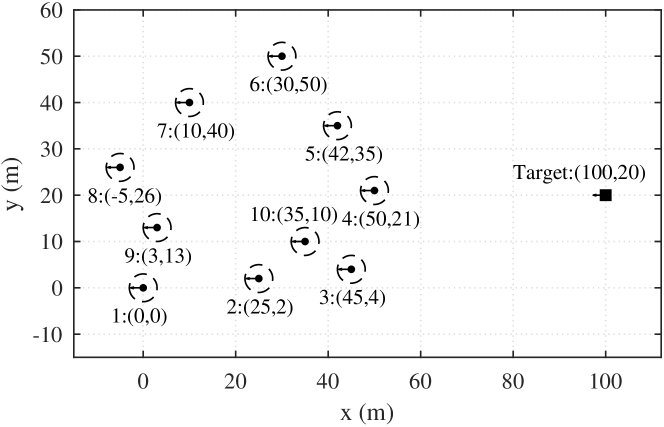
Figure 1: The simulation scenario. The solid dots indicate the networked agents, the solid square denotes the target, and the arrows indicate the speed vector. The dotted circles denote the agent uncertainties. The texts give the agent nominal positions in the form of agent index: $(x,y)$ m.

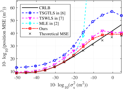
(a)

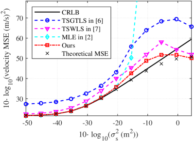
(b)

Figure 2: Performance comparison versus different agent uncertainties, under fixed topology of agents and target for non-LTCO scenarios. (a) Estimation results of moving target position. (b) Estimation results of moving target velocity.

1) Non-LTCO scenarios: The target clock offset is randomly generated from $-10$ to $10$ ns, to simulate the non-LTCO scenarios. Fig. 2 shows the estimation performance comparison versus agent uncertainties $\sigma_{s}^{2}$. We can see that our proposed method significantly outperforms the existing methods. Moreover, the performance of our method can attain the CRLB and consistent with theoretical MSE under small noises, which validates the performance analysis results. TSGTLS and TSWLS perform worse mainly because they do not deeply exploit the nonlinear relationship between target parameters and nuisance parameters. Our method is also robust to large agent uncertainties, while MLE will diverge due to large errors in its coefficient matrix $\mathbf{A}$.

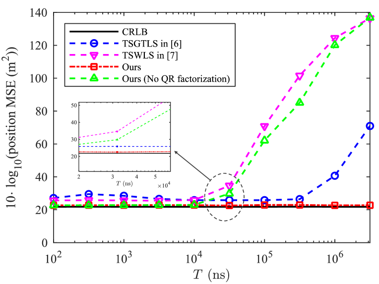
Figure 3: Performance comparison versus different target clock offset, under fixed topology of agents and target.

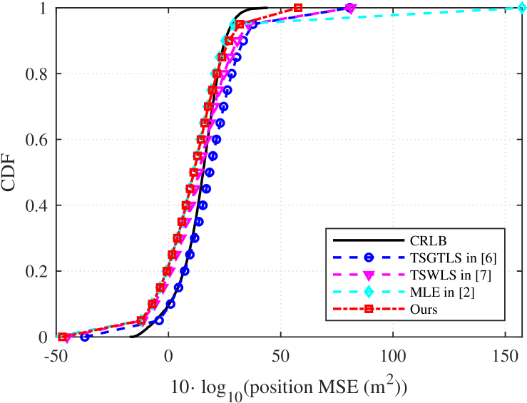
Figure 4: Performance comparison under random topologies of agents and target.

2) LTCO scenarios: We increase the target clock offset to simulate a weak to strong LTCO scenario and fix $\sigma_{s}=-20.5$ dB. We note that when a target cannot access the multi-agent network, it may synchronize its clock via the Internet, in a typical precision of a few milliseconds [16]. When it enters the network, the strong LTCO scenario arises. Fig. 3 demonstrates that our method is robust to strong LTCO scenarios due to the advantage of utilizing the QR factorization, while the existing closed-form solutions fail.

3) Random topology: For further evaluation, we randomly generate the agents and target topology in each independent run, and fix $\sigma_{s}=-20.5$ dB, in non-LTCO scenarios. The agent $x$ and $y$ coordinates are randomly drawn from $0$ to $50$ m, the target coordinates are from $-50$ to $100$ m, and their velocities in all directions are from $-5$ to $5$ m/s. The number of independent runs is $N=10000$. Fig. 4 shows the cumulative distribution function (CDF) of the position MSE. We observe that the CDF curve of our method is steeper for most of the time and can achieve 1 under small position MSE, which confirms that our method performs better than existing methods and is more robust to random localization topology.

The estimation results of clock offset, clock skew and/or target speed lead to the same conclusion, and are not shown here due to space limitations.

VI Conclusion

In this letter, an extended TSWLS method is proposed to localize moving targets with the assistance of a multi-agent network. The position and velocity of the target are jointly estimated using the sequential TOA measurements. Moreover, numerical stability is enhanced to produce valid estimates in LTCO scenarios. Performance analysis and numerical results validate that our proposed method is approximately unbiased and reaches CRLB under small noises. Numerical simulations also show that our method outperforms the existing closed-form solutions in terms of accuracy and robustness, both in non-LTCO and LTCO scenarios.

References

- [1] Q. Wang, W. Zhang, Y. Liu, and Y. Liu, “Multi-UAV dynamic wireless networking with deep reinforcement learning,” IEEE Commun. Lett., vol. 23, no. 12, pp. 2243–2246, 2019.
- [2] Q. Shi, X. Cui, S. Zhao, S. Xu, and M. Lu, “BLAS: Broadcast relative localization and clock synchronization for dynamic dense multi-agent systems,” IEEE Trans. Aerosp. Electron. Syst., pp. 1–1, 2020.
- [3] J. Cano, S. Chidami, and J. Le Ny, “A kalman filter-based algorithm for simultaneous time synchronization and localization in UWB networks,” in Proc. IEEE Int. Conf. Robot. Automat. IEEE, 2019, pp. 1431–1437.
- [4] Q. Shi, X. Cui, S. Zhao, J. Wen, and M. Lu, “Range-only collaborative localization for ground vehicles,” in Proc. 32nd Int. Tech. Meeting Satell. Div. Inst. Navig. ION, 2019.
- [5] M. Angjelichinoski, D. Denkovski, V. Atanasovski, and L. Gavrilovska, “SPEAR: Source position estimation for anchor position uncertainty reduction,” IEEE Commun. Lett., vol. 18, no. 4, pp. 560–563, 2014.
- [6] J. Zheng and Y.-C. Wu, “Joint time synchronization and localization of an unknown node in wireless sensor networks,” IEEE Trans. Signal Process., vol. 58, no. 3, pp. 1309–1320, 2009.
- [7] Y. Wang, J. Huang, L. Yang, and Y. Xue, “TOA-based joint synchronization and source localization with random errors in sensor positions and sensor clock biases,” Ad Hoc Netw., vol. 27, pp. 99–111, 2015.
- [8] J. Tiemann, Y. Elmasry, L. Koring, and C. Wietfeld, “Atlas fast: Fast and simple scheduled tdoa for reliable ultra-wideband localization,” in Proc. IEEE Int. Conf. Robot. Automat. IEEE, 2019, pp. 2554–2560.
- [9] L. A. Romero, J. Mason, and D. M. Day, “The large equal radius conditions and time of arrival geolocation algorithms,” SIAM J. SCI. Comput., vol. 31, no. 1, pp. 254–272, 2008.
- [10] L. A. Romero and J. Mason, “Evaluation of direct and iterative methods for overdetermined systems of toa geolocation equations,” IEEE Trans. Aerosp. Electron. Syst., vol. 47, no. 2, pp. 1213–1229, 2011.
- [11] D. Neirynck, E. Luk, and M. McLaughlin, “An alternative double-sided two-way ranging method,” in Proc. IEEE 13th Workshop Positioning Navig. and Commun. IEEE, 2016, pp. 1–4.
- [12] J. Elson, L. Girod, and D. Estrin, “Fine-grained network time synchronization using reference broadcasts,” ACM SIGOPS Oper. Syst. Rev., vol. 36, no. SI, pp. 147–163, 2002.
- [13] S. M. Kay, Fundamentals of statistical signal processing. Prentice Hall PTR, 1993.
- [14] P. D. Hough and S. A. Vavasis, “Complete orthogonal decomposition for weighted least squares,” SIAM J. Matrix Anal. Appl., vol. 18, no. 2, pp. 369–392, 1997.
- [15] C. Xu and C. L. Law, “Delay-dependent threshold selection for UWB TOA estimation,” IEEE Commun. Lett., vol. 12, no. 5, pp. 380–382, 2008.
- [16] D. L. Mills, “Internet time synchronization: the network time protocol,” IEEE Trans. Wireless Commun., vol. 39, no. 10, pp. 1482–1493, 1991.