BayesicFitting, a PYTHON Toolbox for Bayesian Fitting and Evidence Calculation.
Including a Nested Sampling implementation

Abstract

BayesicFitting is a comprehensive, general-purpose toolbox for simple and standardized model fitting. Its fitting options range from simple least-squares methods, via maximum likelihood to fully Bayesian inference, working on a multitude of available models. BayesicFitting is open source and has been in development and use since the 1990s. It has been applied to a variety of science applications, chiefly in astronomy.

BayesicFitting consists of a collection of PYTHON classes that can be combined to solve quite complicated inference problems. Amongst the classes are models, fitters, priors, error distributions, engines, samples, and of course NestedSampler, our general-purpose implementation of the nested sampling algorithm.

Nested sampling is a novel way to perform Bayesian calculations. It can be applied to inference problems, that consist of a parameterized model to fit measured data to. NestedSampler calculates the Bayesian evidence as the numeric integral over the posterior probability of (hyper)parameters of the problem. The solution in terms of the parameters is obtained as a set of weighted samples drawn from the posterior.

In this paper, we emphasize nested sampling and all classes that are directly connected to it. Additionally, we present the fitters, which fit the data by the least-squares method or the maximum likelihood method. They can also calculate the Bayesian evidence as a Gaussian approximation.

We will discuss the architecture of the toolbox. Which classes are present, what is their function, how they are related and implementational details where it gets complicated.

1 Introduction

1.1 BayesicFitting

The BayesicFitting software package is a PYTHON toolbox for doing Bayesian inference calculations in a simple and standardized way. Given a dataset and a parameterized model, the toolbox can optimize the parameters, obtain standard deviations, confidence regions, and most importantly calculate the evidence for the model. This evidence can be compared with the evidence for other models to decide which model fits best. The option to decide which model is better than another, lifts Bayesian fitting far above the traditional methods.

There are several other Bayesian inference packages available to the scientific community: Bayesian packages in R [1], OpenBUGS [2], Emcee [3], Stan [4]. Or specialized packages for X-ray astronomy: XSPEC [5] and BXA [6]. However, they all miss one or more of the key elements of BayesicFitting: evidence calculation, generic applicability, nested sampling, and ready-made, combinable models.

The BayesicFitting toolbox contains over 100 PYTHON classes, for models, fitters, priors, error distributions, etc. The models can be combined in various ways with each other to form new compound models. Models are discussed in section 6, preceded by the somewhat more abstract concept of problems in section 5. The fitters are explained in section 11. The sections in between are part of NestedSampler, mostly. They are devoted to error distributions (section 7), priors (section 8), engines (section 9), and samples (section 10). After these sections, we discuss quality assurance in section 12. And finally, we present a summary in section 13.

While many fitters, including simple least-squares, are supported by BayesicFitting, the centerpiece of BayesicFitting (and the main focus of this paper) is NestedSampler. It is an independent implementation of the nested sampling algorithm developed by Skilling [7, 8]. NestedSampler is a fully Bayesian algorithm to calculate the evidence and obtain samples from the posterior. Nested sampling is explained in sections 3 and 4. However, we start with Bayes’ rule in section 2.

Interspersed in the text are 3 examples on how to use the toolbox. They do not fit in the running text so they are presented as stand-alone sections called Example: a tea experiment, an exoplanet, and Boyle’s law.

1.2 Pedigree

BayesicFitting started life in the 1990s as a JAVA package inside the Herschel Common Software System (HCSS) [9] of ESA’s Herschel satellite. As a HIFI contribution to the system [10, 11], we elected to write the fitter toolbox, building on 40 years of experience in data modeling for instrument calibration and other data analysis projects.

At the end of Herschels Post-Operations period, maintenance of the HCSS system was suspended. Since this lack of maintenance will unavoidably lead to loss of functionality and eventually to loss of fitness, we decided to translate the toolbox into PYTHON, using NumPy [12], SciPy [13], and AstroPy [14] as basis for relevant and speedy array operations. A small program, j2py [15], adapted and expanded for this purpose, was used in translating the JAVA code to PYTHON. It served mostly to keep in place the class structure with all its methods and inheritances and, very importantly, the documentation. Still, all code lines had to be inspected, corrected, and pythonized. By now BayesicFitting is larger and more powerful than the HCSS fitter toolbox ever was.

As part of HCSS, the fitter toolbox was used in the software pipelines of the 3 instruments onboard the Herschel satellite. The pipelines processed all data taken by Herschel whether astronomic observations or calibration measurements; even ground-based instruments tests needed to pass through the pipelines [9] without failure. Consequently, the fitter toolbox was extensively tested in an astronomical environment. By carefully translating the JAVA-based fitter toolbox we introduced extra security into the new PYTHON-based BayesicFitting toolbox.

As an interpreted language PYTHON is not very fast. However, all array operations are relegated to the NumPy and SciPy packages which are written in C-code, compiled, and linked. Most of the CPU is spent while calculating the likelihood function over the data arrays, in compiled code. More speed can be obtained by linking a threaded version of NumPy, SciPy, and the underlying BLAS/LaPack libraries. None of the classes is using global constants or even class attributes, so each object is an independent entity.

1.3 Notation

BayesicFitting is written in PYTHON as a collection of classes. These classes have names in CamelCase. In this paper, classes are written in boldface. So Model is a class inside BayesicFitting built around a mathematical model. There is no sharp dividing line, however. Notations might mix. Classes with similar endings belong to the same family tree of Models, Engines, Priors, etc. These latter ones are the central members of the hierarchy. Interaction with other classes is addressed through them.

Actual PYTHON code is written in teletype, either inline or in small boxed code blocks. Due to space limitations and for readability the PYTHON code is “stylized”. E.g. the reference to self is often omitted where it is obvious.

1.4 Availability

BayesicFitting is released in the public domain under the GPL3 license. It can be obtained from

PyPi	https://pypi.org/project/BayesicFitting
GitHub	https://github.com/dokester/BayesicFitting
zenodo	https://zenodo.org
	doi:10.5281/zenodo.2597200.
home	https://bayesicfitting.nl

2 Bayes’ Theorem

This is not the place to expound Bayesian Statistics and Inference. We refer the interested reader to textbooks such as [16, 17, 18]. On a fundamental level, Bayes’ theorem is the reason we can say something about parameters when we only know something about data.

In this vein, we introduce Bayes’ theorem to update knowledge, as-is: a relation of (densities of) probabilities, $p$, about statements, $a$ and $b$ in the presence of background information, $I$.

$$p(a\,|\,b,I)=\frac{p(a\,|\,I)\,p(b\,|\,a,I)}{p(b\,|\,I)}$$ (1)

In terms of model inference, this transforms into a relation of probability densities between parameters, $\theta$, data, $d$, and a model, $m$.

$$p(\theta\,|\,d,m)=\frac{p(\theta\,|\,m)\,p(d\,|\,\theta,m)}{p(d\,|\,m)}$$ (2)

Each of these elements has its own symbol and a name. In words, we can write

$$\mbox{posterior}=\frac{\mbox{prior}\times\mbox{likelihood}}{\mbox{evidence}}.$$ (3)

As the prior and the posterior are both distributions we give them the same symbol $P$, where the prior gets a subscript of 0 to indicate it is the probability we start with. By multiplying it by the likelihood, $L$, and dividing by the evidence, $Z$, we obtain the final probability, $P$, the posterior

$$P=\frac{P_{0}\times L}{Z}$$ (4)

To emphasize that Bayes’ rule updates our knowledge, we can borrow notation from computer languages.

$$P\,*\!\!=L\,/\,Z$$ (5)

It also underlines that the posterior of one problem can be the prior of the next.

posterior

The posterior distribution is a multi-dimensional distribution of the parameters given the model and the data. The posterior represents our updated knowledge of the parameters after taking into account the data. Parameter averages, standard deviations, and other items can be extracted from the posterior.

prior

The prior distribution is the probability of the parameters given the model without the (present) data. They are educated guesses of the ranges over which the parameters of the model might vary. There is a lot of (intentional) confusion about priors. But only theoreticians can imagine a model where they (pretend to) have no knowledge at all about the extent of the parameters. Real practitioners never have that problem. There are always limits. And in most cases, the data overwhelm the specific choice of the priors anyway. If not, the data bear little information about the problem at hand, either by paucity or by irrelevance. The prior could also be the result of a previous inference problem. Bayes’ theorem updates knowledge.

likelihood

The likelihood is the calculated probability of the errors, the differences between data and model, given a set of parameters. The choice for the error distribution to be used depends on the problem itself and on the data.

evidence

On the face of it, the evidence is just a normalization factor, needed to have to probabilities of the posterior integrate to 1.0. And this is indeed how it is calculated:

$$Z=\int P_{0}\,L\,d\theta$$ (6)

However, it can play a much more important role as the probability of the model given the data. Hence its name: evidence. It shows how good one model is with respect to another.

We write equation 1 for model and data only; the probability of the model given the data.

$$p(m\,|\,d)=\frac{p(m)\,p(d\,|\,m)}{p(d)}$$ (7)

The normalization factor, $p(d)$, cannot be assessed, as it would have us integrate over all possible models. However, if we restrict our universe to a small number of models, say 2, we can write the odds ratio between model 1 and model 2 as

$$\frac{p(m_{1}\,|\,d)}{p(m_{2}\,|\,d)}=\frac{p(m_{1})}{p(m_{2})}\frac{p(d\,|\,m_{1})}{p(d\,|\,m_{2})}$$ (8)

Assuming that we have no preference for either $m_{1}$ or $m_{2}$ i.e. the prior odds ratio is 1.0, we can determine which model is better than the other and by how much. The second factor, the evidence ratio, is also called the Bayes factor, $B_{12}$.

This possibility for favoring one model over another is the most important feature that lifts Bayesian inference over the more traditional versions of inference. The papers [19, 20, 21, 22, 23, 24] are all about problems that could only be solved by selecting the best model. And never, in our experience, did it fail Laplace’s adage: “Probability theory is nothing more than common sense reduced to calculation.”

3 Nested Sampling

Nested sampling is an algorithm developed by Skilling [7] designed to calculate the evidence, $Z$ of equation 6. Unlike other Markov Chain Monte Carlo (MCMC) algorithms it does not need a “burn-in” and it has a well-defined stopping criterion. While calculating the evidence, nested sampling produces samples, randomly drawn from the posterior distribution.

The algorithm initializes an ensemble of N walkers, points in parameter space, randomly distributed over the prior. For all walkers, the log-likelihood, $\log\!L$, is calculated.

In subsequent iterations the walker with the lowest likelihood, $\log\!L_{low}$ is stored in a sample list, supplemented with a weight proportional to its contribution to the posterior. The walker is removed from the ensemble. A new walker is generated, randomly distributed over the prior, that has a $\log\!L$ that is higher than the $\log\!L_{low}$ of the discarded walker. This way we are climbing the likelihood mountain. As each walker represents 1/N part of the available remaining space we can numerically integrate the likelihood in successive steps. The prior is taken into account by the generation of the walkers via importance sampling. When the top of the likelihood is reached, the integral is complete: the evidence is obtained.

The nested sampling algorithm can be explained in one small paragraph. Hereafter we will address our general-purpose implementation of nested sampling.

4 NestedSampler

Suppose we have a problem containing parameters and data that bear relevance to these parameters. The problem could be a classic regression problem or something more complicated, as addressed in section 5.

NestedSampler takes the problem and applies the nested sampling algorithm to obtain the evidence, and posterior in the form of a list of samples. The algorithm, which is called with NestedSamplers sample() method, can be split into 7 steps. See Sivia [16] for more details.

1. Initialize an ensemble of N walkers, randomly distributed over the parameter space according to the priors. Calculate the $\log\!L$, the log of the likelihood for each of the walkers.

   During the iterative process, the space occupied by the walkers shrinks on average as an exponential function

   $$X(i)=\exp(-i/N)$$ (9)

   where $i$ is the iteration number.

2. Find the walker with the lowest log-likelihood, $\log\!L_{low}$, the worst in the ensemble. The width for which the $\log\!L_{low}$ is valid is the amount of shrinkage in the iteration. It equals the difference between subsequent $X$’s.

         logWidth = log( X(i-1) - X(i) )     

3. Copy the worst walker, properly weighted, to the list of samples. The weight of the sample is calculated as the product of the likelihood and the width of the area for which it is valid.

         logWgt = logL + logWidth     

4. Update the developing integral for the evidence, Z, by adding the weight. As we do our calculations in the log we need the function numpy.logaddexp(). Similarly, update the Kulback-Leibler information, H, also known as the Kulback-Leibler divergence.

   $$H\approx\sum_{i}\frac{W_{i}}{Z}\log\frac{L_{i}}{Z}$$ (10)

         logZn = numpy.logaddexp( logZ, logWgt )   # update Information, H   H = ( math.exp( logWgt - logZn ) * logL +         math.exp( logZ - logZn ) *         ( H + logZ ) - logZn )   logZ = logZn     

5. Remove the worst walker from the ensemble.

6. Duplicate a randomly selected walker from the remaining ensemble. The duplicated walker needs to be moved around while its $\log\!L$ stays higher than that of the discarded walker until it is randomly distributed over the prior. As the other walkers were already randomly distributed and the new one is just made so, we have a new ensemble that is randomly distributed over a shrunken volume while all its $\log\!L$s are above the limit set in step 2. The exploration of the available space is done by the engines of section 9. This step is the hardest of them all. It is called the “Central Problem” of nested sampling [25].

7. Go back to step 2 until done. While the remaining space is slowly but exponentially decreasing, the likelihood is increasing until its maximum is reached. While the likelihood stays at its maximum, the available volume continues to go down. The product of these two counterbalancing trends produces a hump-like behavior in the contributions to the integral of the posterior. When the hump is passed and the contributions are back to (almost) zero it is time to stop. More strictly the iterations are stopped when

         if iteration > 2 * N * H :       break     

When the iteration is stopped, the remaining walkers are copied to the list of samples. The sample() method returns the evidence, or more specificly, the $\log_{10}$ of the evidence. This $\log_{10}Z$, multiplied by 10, can be viewed as decibel when comparing models. From the samplelist, obtained as the attribute samples from NestedSampler, all kinds of statistics can be derived about the problem.

4.1 Explorer

The Explorer addresses step 6 in the list above. It calls the list of Engines in random order until enough randomness is achieved. This is a balance between efficiency and thoroughness. Efficiency for speedy calculations and thoroughness for losing correlation with the starting point. Experience showed that between 5 and 10 valid steps are enough.

The Engines can be put in separate threads if we are exploring more than one Walker per iteration to parallelize and speed up the calculations.

4.2 PhantomSampler

The PhantomSampler is quite similar to the NestedSampler except that it uses part of the phantoms (see section 9.7) to speed up the calculations. Each iteration several Walkers with the lowest $\log\!L$, are removed from the ensemble and copied to the SampleList. Only one Walker is evolved, subject to a $\log\!L_{low}$ equal to the best of the removed ones. The other Walkers are replaced with phantoms randomly chosen from the evolved path.

5 Problem

A Problem is a class that is defined by data, $D$, parameters, $\theta$, and a forward transform from parameters to mock data i.e. the data values according to the problem. From this, it should be possible to calculate a measure of distance between real data and mock data and from that the likelihood.

Data, parameters, and the transform are stored in the Problem. Optionally, weights can be stored too. Throughout the BayesicFitting toolbox weights are defined as equivalent to a “quantity of data”. A weight of $w$ is equivalent to having $w$ of the same data. Of course, a weight could be the inverse square of a standard deviation obtained earlier for the data-point, but it does not necessarily need to be. Weights are more general. E.g. a weight of 0 results in the omission of the data-point from the solution which is impossible when using standard deviations.

Traditionally the data consists of independent variables, $x$, which are known without error, and dependent variables, $d$. The transform is defined in a Model class as a parameterized mathematical function, $F$. Given a set of values for the parameters, the function calculates mock data, $y=$ $F(x\!:\!\theta)$. The mock data is the Models guess for $d$. The real data and the mock data go into the ErrorDistribution to calculate the likelihood. The traditional case, i.e. only errors in the dependent variable, $y$, is called a ClassicProblem. It is the default and it does not have to be declared.

Another option is an ErrorsInXandYProblem where the $x$ variables are known with similar (un)certainty as the $d$ variables. An example in case is a color-color diagram in astronomy where there are color values on both axes; one not more certain than the other. We have to define extra unknown quantities, $u$, one for each value of $x$. The $u$ need to be estimated along with the parameters $\theta$. As we are not directly interested in them, they are called nuisance parameters. The nuisance parameters need priors too. Here we would advise using a GaussPrior centered on the $x$ values. We don’t want the $u$ to stray too much from the corresponding $x$. Both pairs, $(d,y)$, and $(u,x)$ go into the ErrorDistribution to calculate the likelihood. In these problems, we have more parameters to estimate than there are data. In Bayesian inference, this is not a problem because the priors stabilize the solution.

In a MultipleOutputProblem, the data variable $d$ has more than 1 dimension. Such is e.g. the case in fitting stellar orbits as they appear on the sky. Or when $d$ is the outcome of a football match [22]. Obviously, the Model needs to produce mock data of the same dimensionality as the data, $d$. The MultipleOutputProblem flattens the multi-dimensional output to a one-dimensional array, so it can be passed to the ErrorDistribution.

The final Problems we would like to discuss are discrete. The probabilities in equation 2 are not densities because the possible configurations are discrete, each having its own likelihood value. Consequently the integral of equation 6 reverts to a sum over all configurations. However, the number of options is so large that they cannot sensibly be enumerated. We treat the sum as an integral that ironically, is calculated by the NestedSampler numerically, as a sum.

The first discrete problem is the EvidenceProblem. We lift the nested sampling to the next level. Instead of calculating the $\log\!Z$ of equation 2, we calculate equation 7. As equation 7 only functions as a comparison between different models, we need a way to generate models. The Model class has children which are Dynamic and/or Modifiable, see section 6.5. They have a dynamic number of components and hence of parameters, or their internal structure can be modified at a fixed number of parameters. In an EvidenceProblem the optimal number of components and internal structure is found along with its preference over other configurations.

OrderProblems try to find a certain order in the elements of its problem domain. E.g. a school schedule; which lessons have to be presented by what teachers to what sets of pupils in which classrooms and when [28]. Probabilistic results do not work in this case. A singular “best” result is what we are looking for. Our choice for the likelihood is the exp of the negated cost function which weighs the misfits in the schedule. This likelihood is unnormalized as normalization would entail summation over all configurations, which we cannot do because of its multitude. The normalization factor will be taken up in the evidence.

The traveling salesman also fits in this problem category, the cost function is now the length of the path traveled.

All these problems can be addressed in NestedSampler, although to solve the OrderProblem specialized ErrorDistribution and Engines need to be written.

6 Models

The Models are a large hierarchy of classes centered around Model itself. In figure 1 the inheritance tree of models is schematically shown. At the top of the tree GaussModel, PolynomialModel and SineModel are shown as representatives of all simple models that inherit from Model. Collectively we will indicate them as SimpleModels.

These SimpleModels inherit from Model and subsequently from FixedModel and BaseModel. Actually, a SimpleModel is mostly a specialization of BaseModel at the root of the tree. However, as all interactions with other classes are organized via Model, the inheritance line from BaseModel to each SimpleModel has to go through FixedModel, Model, and some auxiliary classes, not mentioned here. This way the SimpleModels are Models on their own and more complicated constructs built from SimpleModels are Models too.

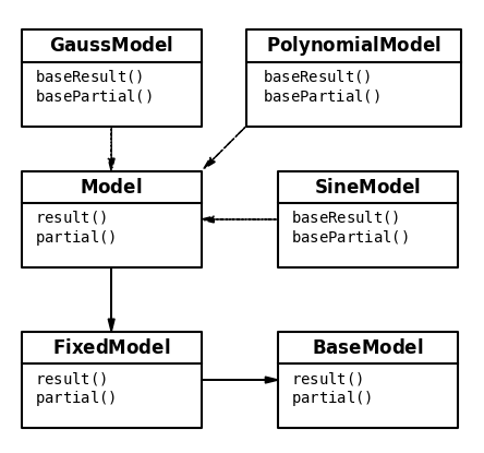
Figure 1: Schematic hierarchy of the model classes. Only a small selection of classes that inherit from Model is shown. The arrow points to the parent class it is inheriting from.

6.1 BaseModel

The BaseModel is an abstract (or base) class that should not be instantiated directly. It comes to life when a SimpleModel is invoked. BaseModel defines attributes and methods relevant to simple models. Attributes like the number of parameters, the dimensions of input and output, parameter names, whether some parameters need to be positive or non-zero. The priors on the parameters are stored here too as a list of Priors. And methods to act upon these attributes.

Other methods like result() and the partial derivative to the parameters partial() directly call baseResult() and basePartial() in the relevant SimpleModel. As is the __str__() method which directly calls the baseName() method of its ultimate great-grandchild.

6.2 SimpleModels

A SimpleModel is the concrete realization of the BaseModel. It is built around a mathematical function, $F(x\!:\!\theta)$, implementing its result, its partial derivatives to each of the parameters, and its derivative to $x$. There are more than 50 different SimpleModels in the toolkit. They can be used as-is or as building blocks for more complicated models as described below.

What exactly constitutes a simple function is a matter of taste and efficiency. Sometimes a more complicated function, which could in principle be constructed from building blocks, is better constructed as one class. At least it can be done more efficiently.

6.3 FixedModel

The FixedModel is an abstract class too, in which one or more parameters is replaced by either a fixed, constant number or by the results of another Model. The fixed model loses one parameter for each fixed one and possibly gains the parameters of the replacing models, which are placed at the end of the parameter list.

When replacing a parameter with the results of another model there are no broadcasting problems as the length of the output arrays, $y$, are equal to those of the input, $x$. Partials and derivatives are calculated using the chain rule.

A simple model can only be “fixed” at its construction and it remains fixed during its lifetime. For all practical purposes a FixedModel acts as a single unit: a simple model.

      print( PolynomialModel( 2 ) )   Polynomial: f(x:p) = p_0 + p_1 * x + p_2 * x^2   print( PolynomialModel( 2, fixed={1:1.5} ) )   Polynomial: f(x:p) = p_0 + 1.5 * x + p_1 * x^2     

The PolynomialModel of order 2, has 3 parameters. When we fix the slope at 1.5, it has 2 parameters left: for the constant and for the $x^{2}$.

6.4 Compound Models

Every Model has a link either to None or to another Model. None indicates the end of the linked list. Upon creation, all SimpleModels have a None link.

Linked Models have an associated list of operators, one for each link, which tells how the results of the next model operate upon the previously obtained results. Operators can be one of $+$ (addition), $-$ (subtraction), $*$ (multiplication), $/$ (division) or $|$ (pipe). The first 4 do the obvious thing: they add, subtract multiply or divide the results of the two Models to obtain a new result. The pipe uses the results obtained by the Model on the left-hand side, as input of the Model on the right-hand side. Like a UNIX pipe.

The linked list is stepped through in a recursive way for all methods that need information from each of the constituent Models. As an example, we show in figure 2 how results for a compound model are obtained.

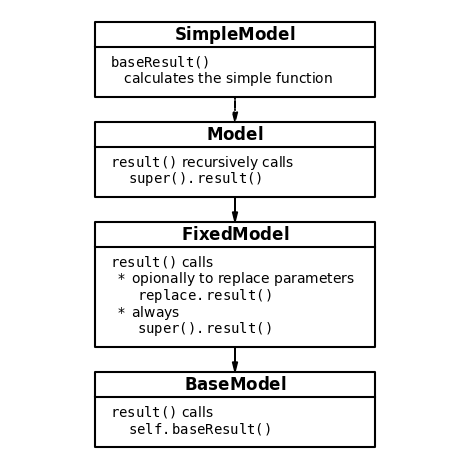
Figure 2: Calling sequence of the result() method, explained in the text below.

When the method result() is called in a compound model, it starts at the first SimpleModel in the chain. A SimpleModel does not have a result() method, so it falls through to Model. The result() method in Model recursively addresses the elements of its linked list. For each element, starting at itself, it calls the result() method in FixedModel. FixedModel starts looking for parameters that might be replaced by another Model. This might be a full-fledged compound model so it calls result() in another Model. When the results have returned it looks for other parameters that might have been replaced by constants and calls result() in BaseModel with the reconstructed parameters. This last method directly calls baseResult() in the relevant SimpleModel. All recursively found results are operated upon according to their associated operators.

Two linked Models form a new unit which has (virtual) brackets around the operation. Its compound results are obtained before progressing down the chain. This might result in counterintuitive results that ignore normal operator preferences. E.g. m1 + m2 * m3 is evaluated as (m1 + m2) * m3. However by reordering the chain or inserting extra brackets or separate evaluation of a subchain the intuitive outcome can be obtained.

      m4 = m2 * m3             # m4 is a new unit   mdl1 = m1 + m4           # == ( m1 + ( m2 * m3 ))   mdl2 = m2 * m3 + m1      # equivalent to mdl1   mdl3 = m1 + ( m2 * m3 )  # equivalent to mdl1     

6.5 Dynamic and Modifiable

Dynamic and Modifiable are base classes that can be used as extra parent classes for Models that can change its number of parameters or modify its internal structure. As an example we have a splines model where the number of knots can be changed (Dynamic) and/or the location of the knots can be modified (Modifiable).

Upon instantiation of any SimpleModel the init method of its parent is called via super().__init__(). For a dynamic model that inherits from 2 (or 3) parent classes, it is not obvious which class super() points to. The parent classes need to be called by name.

      class SomeModel( Modifiable, Dynamic, Model ):       def __init__( self ) :           Modifiable.__init__()           Dynamic.__init__()           Model.__init__()     

7 ErrorDistribution

When we have selected a model and a set of (trial) values for the parameters we can calculate mock data, $y=$ $F(x\!:\!\theta)$. We manipulate the parameter values such that mock data and measured data are as close as possible. Historically how to measure this closeness, was not all that obvious. Gauss minimized the squared distances, giving rise to the well known “least-squares” (or $\chi^{2}$) method. Laplace favored minimizing the absolute value of the distances. Both are valid for certain kinds of errors. As the least-squares methods proved easier to calculate it was for a long time the method of choice.

In probability theory, we want to obtain the probabilities for the distances between mock and measured data. Error distributions will calculate the probability of these distances, resulting in the likelihood term in equation 2: $p(d\,|\,\theta,m)$.

When we use the normal (or Gaussian) probability density function as the distribution of the errors, we get for each individual data point, $x_{k}$, and optionally an associated weight, $w_{k}$, the calculated probability of its residual.

$$\mathcal{L}(x_{k})=\sqrt{\frac{w_{k}}{2\pi\sigma^{2}}}\exp\left(-0.5w_{k}\left(\frac{y_{k}-d_{k}}{\sigma}\right)^{2}\right)$$ (12)

The $\sigma$ is a parameter of the error distribution and can be estimated independently as a hyperparameter of the problem. The optimal $\sigma$ represents the noise scale, i.e. the standard deviation of the residuals: data minus optimal model.

If the errors are independent of each other, the likelihood is the product of the individual contributions over all data points.

$$L=\prod_{k}\mathcal{L}(x_{k})$$ (13)

As we perform our calculations in the log, equation 13 reverts to the sum over the log of the individual contributions. The log of the (normal) likelihood of the errors is equal to the sum of the squares of the errors. Maximizing the likelihood is equivalent to minimizing the sum of the squares, or equivalent to the least-squares method.

So we see that least-squares is an approximation of Bayesian fitting. When we would have taken the Laplace probability distribution as likelihood, we would have obtained something equivalent to Laplace’ method of minimizing the absolute deviations. His method is a Bayesian approximation too.

Conversely, with the BayesicFitting toolbox, these traditional fittings can be done as well.

7.1 ErrorDistribution classes

Central in the tree of error distribution classes is ErrorDistribution. It stores hyperparameters that might be present and might be added to the list of parameters to be estimated. These hyperparameters of course have their own Priors. ErrorDistributions act upon a Problem and parameters, $\Theta$ which includes the parameters of the model, $\theta$, and the hyperparameters of the error distribution.

Which particular error distribution is needed, is a choice of the practitioner depending on the experiment at hand. However, this is not the place to discuss these choices. We only present the options.

For counting problems, we provide the PoissonErrorDistribution. For median-like solutions with the 1-norm, there is the LaplaceErrorDistribution, for the 2-norm, the good old GaussErrorDistribution, equivalent to least-squares and for the $\infty$-norm we supply the UniformErrorDistribution where the maximum of the residuals is minimized. Other norms can be made with the ExponentialErrorDistribution, setting the power as norm. This power is an extra hyperparameter in addition to the scale hyperparameter that all norm-ed error distributions have. For categorical problems, we have the BernoulliErrorDistribution.

And finally, for EvidenceProblems, there is the ModelDistribution. It provides the likelihood term in equation 7, $p(d\,|\,m)$, which is the same as the evidence term in equation 2. ModelDistribution calculates the evidence either by running NestedSampler or as a Gaussian approximation using one of the Fitters.

7.2 Mixed Error Distributions

A MixedErrorDistribution combines the weighted contributions of two other distributions, either of the same class or different. It can be used in situations where there are spurious outliers, excursions much larger than the others. In such cases, equation 13 is changed into

$$L=\prod\,\lambda\mathcal{L}_{1}(x_{k})+(1-\lambda)\mathcal{L}_{2}(x_{k})$$ (14)

Again, as the individual contributions are only known in the log we have to use the logaddexp() method from NumPy. The mixing factor, $\lambda$, can have values between 0 and 1. It is another hyperparameter of the MixedErrorDistribution next to the ones from both constituent distributions.

Because of these requirements in MixedErrorDistribution, the summation over the log-likelihood contributions of each data point is delegated to the base class ErrorDistribution.

7.3 Constraints

The space available to the parameters is restricted by their priors. By construction the parameters are orthogonal. However, in real life, restrictions on combinations of parameters are also possible. In these cases, a constrain method needs to be defined which excludes certain regions of the priors (exclusion sampling).

7.4 Cost Functions

Nested sampling is a very general method to integrate a multidimensional exponentiated function. It does not necessarily need to be a likelihood function. It could be the length of the travels of the salesman or the number of misfits in a school schedule [28]. The likelihood proxy can be each of these quantities in the negative and exponentiated. Generally, these are known as cost functions. Cost functions are the unnormalized likelihoods of OrderProblems, see section 5.

In OrderProblems the domain of the parameters is not continuous; it consists of a (large) number of options. N! in case of an N city route and for a typical Dutch secondary school it is $10^{3800}$. Consequently, there is no guarantee that nearby the copied point a valid new one can be found. We have to search for new Walkers until we find a valid one.

8 Priors

To calculate the evidence we need to integrate the product of likelihood and prior over the parameters. Nested sampling performs the calculation by smart sampling of the posterior. The prior is taken into account by importance sampling.

For this purpose all priors need to have a pair of methods domain2Unit(), the cumulative distribution function (CDF) and unit2Domain(), its inverse (iCDF). When one takes a random value, uniformly between 0 and 1, the inverse CDF transforms it into a random value from the prior. And the CDF can transform any parameter value back into unit space.

The continuity of CDF and iCDF ensure that we can sample from the prior in the vicinity of a given parameter value. We transform the boundaries of the vicinity to the unit range, find a uniformly distributed value within the unit boundaries and transform that value back to the parameter domain. We need this in the next section 9 about engines.

8.1 Limits

Some priors need limits to properly integrate to 1.0, like UniformPrior and JeffreysPrior. Others might be limited by choice. This limitation is handled in Prior. When limits to the priors are provided we define in the unlimited domain the minimum and range in the unit-space, obtained from the lowLimit and highLimit in domain-space.

      umin = domain2Unit( lowLimit )   uran = domain2Unit( highLimit ) - umin     

We manipulate the calling order of unit2Domain() and domain2Unit() methods which resolve to the methods in the specific prior, such that they first pass through the limited versions.

      self.baseDomain2Unit = self.domain2Unit   self.baseUnit2Domain = self.unit2Domain   self.domain2Unit = self.limitedDomain2Unit   self.unit2Domain = self.limitedUnit2Domain     

Now the methods domain2Unit() or unit2Domain() are renamed to their base variant and calls to domain2Unit() or unit2Domain() will resolve to the limited versions.

      def limitedDomain2Unit( self, dval ) :      return ( baseDomain2Unit( dval ) - umin ) / uran     def limitedUnit2Domain( self, uval ) :      return baseUnit2Domain( uval * uran + umin )     

After this manipulation, any call to domain2Unit() goes to limitedDomain2Unit() in Prior, which subsequently calls baseDomain2Unit(), a renaming of domain2Unit() in the specific prior. Similar for unit2Domain().

8.2 Circular

Some parameters are by nature periodic, like phases. They need a circular prior. This is also arranged in Prior. Any prior which is symmetric, $p(\mu-x)=p(\mu+x)$ for some central value, $\mu$, can be made circular.

      self.domain2Unit = self.circularDomain2Unit   self.unit2Domain = self.circularUnit2Domain     def circularDomain2Unit( self, dval ) :      return ( limitedDomain2Unit( dval ) + 1 ) / 3     def circularUnit2Domain( self, uval ) :      return limitedUnit2Domain( ( uval * 3 ) % 1 )     

The first method places the unit domain in a [1/3,2/3] box, so excursions over the edges are possible, while the second method expands it to [0,3] and then only the fractional part is kept. Overflow and underflow out of the original unit box is circled to the other side. The edges i.e. the limits, need to be set so that the prior value at the low limit is continuous to the prior value at the high limit.

8.3 Computation

Priors that have in theory an infinite domain are nonetheless confined in practice. These priors need to die out toward infinity, some faster than others. At a certain moment, the values become indistinguishable from 0. In table 1, the computational boundaries of the domain are given for a number of Priors. When x (here the scaled distance to the center) is larger than the values given, the Prior is essentially 0. No steps can be taken beyond them, so no solution will be found there.

Prior	math	boundaries
GaussPrior	$\exp(-0.5x^{2})$	[-6, 6]
LaplacePrior	$\exp(-|x|)$	[-36, 36]
ExponentialPrior	$\exp(-x)$	[0, 36]
CauchyPrior	$1/(1+x^{2})$	[-1e16, +1e16]

Table 1: Computational boundaries for some unbound Priors using 8 byte floats.

Attractive as GaussPriors are as conjugate to the normal distribution, they are also dangerous. They can only be explored to 6 unit lengths from its center. This is not a mathematical limitation, but a computational one caused by the use of 8 byte floats in normal present day computers

9 Engines

The Engines are the classes where the Walkers are moved around according to their Prior until they have found a new random position, that is still higher than $\log\!L_{low}$. It is easily said but much harder to accomplish. Good exploration is needed to get a solid estimate of the evidence integral. When exploring too much in the high likelihood regions the evidence will be too high. And when too much time is spent in the outskirts the evidence is too low.

All Engines transform the parameters of a Walker that need to be randomized, to unit space, using the domain2Unit() method from the Prior. They select steps in unit space in a uniformly random way. The Prior method unit2Domain() is used to transform the steps to the parameter domain. This way all steps are always distributed according to the Prior of the parameter.

We determine the step size by transforming the maximum and minimum values of the parameters, taken over the ensemble to unit space. There it forms a rectangular container box that encompasses the present ensemble. The box is used as a proxy for the available space in which can be stepped. The size of the steps scales with this.

As we start our Walker by copying a valid one and the likelihood is continuous, we can always find a new position nearby or far.

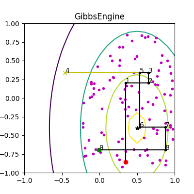
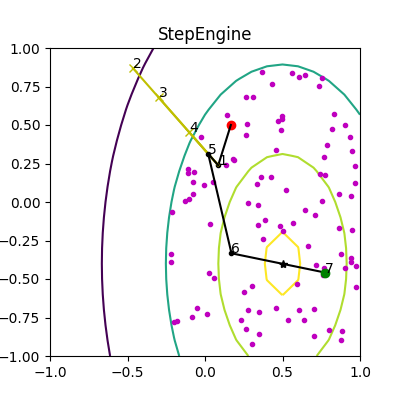
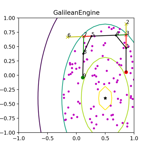
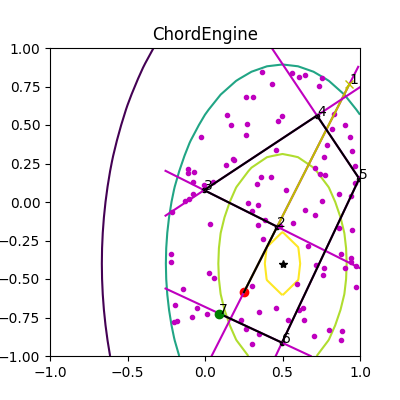
Figure 3: Operation of 4 Engines on an arbitrary PolynomialModel of order 1. The axes are the 2 parameters of the problem, both with UniformPriors between -1 and 1. In all figures the contour of $\log\!L_{low}$is the mint one that encompasses the complete ensemble the 100 purple points. The engine starts at the red point and steps via the numbered points to the final green one. The black points are phantoms. The yellow excursions outside of the mint countour are failed points.

In figure 3 one operation of the 4 engines discussed here, is displayed. It regards a simple linear Problem with only 2 parameters for easy display. An ensemble of 100 Walkers is shown as purple dots. For reference, some contours of equal $\log\!L$ are shown. The one in mint encompassing the whole ensemble, is the present contour of $\log\!L_{low}$. Of course, the exact location of these contours is not known at any time during the operation of the Engine. Here it is shown for reference only. Each Engine starts at a copy of an existing Walker, shown as the big red dot. The Engine moves the point in (numbered) steps to its final position, the big green dot. Black dots mark acceptable (valid) steps as they are within the $\log\!L_{low}$ contour. Yellow dots are steps outside the contour and are rejected (invalid). Details on the individual Engines are discussed below.

For all Engines it is of paramount importance never to accept an invalid location, not even temporarily. Once outside it can be very difficult the get back inside, especially in a high-dimensional parameter space.

9.1 GibbsEngine

Traditionally there is Gibbs sampling, here implemented as GibbsEngine. It moves one parameter at a time by a random amount. If the new likelihood is above $\log\!L_{low}$ the step is valid and the Walker moves on. If not, the step size is decreased until it is accepted. The downside of Gibbs sampling is that is moves one parameter at a time and it performs a random walk. Performance scales with the number of parameters and it moves slowly from its original position. In 2 dimensions, as shown in figure 3, it looks fine. The disadvantages don’t show much. In more dimensions the parameters are addressed in random order; in two dimensions that does not work nicely.

9.2 StepEngine

A slightly more efficient way is the StepEngine. It also does a random walk but it moves in a random direction. All parameters are stepped at the same time. When the step goes outside the valid area, like step 2 in figure 3 it is decreased, first to 3 then to 4, and finally to 5 where it finds a valid position. In this example, the StepEngine looks efficient and simple. In much more dimensions the chance to step outside increases when we take steps of the size shown here. We have to revert to more, smaller steps. However, it is still a random walk that progresses by the square root of the number of steps.

9.3 GalileanEngine

The GalileanEngine is an independent implementation of an algorithm by the same name, designed by Skilling [29]. It tries to amend the disadvantages of both the GibbsEngine and the StepEngine. It selects a step in a random direction vector, $v$, and proceeds along that direction for as long as it is successful. When ultimately a step fails ($<$$\log\!L_{low}$) it tries to mirror on the $\log\!L$-surface to get back into valid space. In figure 3 position 2 (and also 6) finds itself outside the valid area defined by $\log\!L_{low}$. If it mirrors at position 2, it might not return into valid space. However, when we withdraw to position 1 to mirror, we are in danger of undersampling the border regions.

To approximate the position of the $\log\!L_{low}$ surface on the line (1,2), we interpolate from the $\log\!L$ at 1 to the $\log\!L$ at 2, at $\log\!L_{low}$to obtain position 3. This interpolation may not yield the exact location $\log\!L_{low}$, it is closer. There is more chance that mirroring will indeed get us back into valid space. For mirroring we need to alter the present directional vector, $v$.

$$v^{\prime}=v-2dL\frac{(dL.v)}{|dL|}$$ (15)

$v^{\prime}$ is the new stepping vector and $dL$ is the partial derivative of $\log\!L$ to the parameters, $dL=\partial\log L/\partial\Theta$; and $(dL.v)$ is the inner product with $v$. The part of the step outside valid space, is taken in the mirrored direction, here to 4 (and 8). Stepping is continued in the new direction.

When mirroring is not successful we have to back up and retrace our steps in the reverse direction: $v^{\prime}=-v$. To all steps a 10% random disturbance is added, if only to avoid exactly retracing our steps back to the starting point.

The GalileanEngine is the engine of choice for intermediate and large-sized problems. It has none of the disadvantages of GibbsEngine or StepEngine. It can take small steps but as it moves in one direction it quickly traverses the available space to find a new random spot. The only disadvantage is that it needs the partial of $\log\!L$. All existing Models and ErrorDistributions have built-in methods for calculating analytical partials. When some future implementation omits these analytical partials, numeric calculations will automatically kick in.

9.4 ChordEngine

The ChordEngine is an independent implementation of the Polychord algorithm as described in [30] or the Hit-and-Run algorithm of [25]. In unit space it draws a randomly oriented line through the present point and extends it until it reaches outside the valid space, yielding a start point and an endpoint. In figure 3 the purple lines extending from each point reach into invalid space or until the edge of the unit box. On this segment, a random point is selected. When it is valid ($>$$\log\!L_{low}$) it is the new point. Otherwise, either the start point or the endpoint is replaced by the new invalid point. And we select another random point on the new segment. Until we have a valid point.

In figure 3 the first point on the random line through the starting point (red), turns out to be invalid after which we fall back to point 2 in valid space. Subsequent lines are made orthogonal to each other for as long as that is possible. In this 2-dimensional problem, the lines are orthogonal at even points only. At each next point, the possibilities for orthogonality are exhausted and a new random direction is found.

The ChordEngine does not need the partial derivatives to $\log\!L$ which is a bonus. However, it needs to extend the lines until they are in invalid space which in principle are extra likelihood calculations. However, our knowledge of the container box of the present ensemble helps here. We assume that once the line is outside the box, it reaches into invalid space, without further checking.

By default, NestedSampler employs the GalileanEngine and the ChordEngine in a random order.

9.5 BirthEngine and DeathEngine

Dynamic Models need extra Engines to increase or decrease the complexity of the model which manifests itself in the number of parameters the model has. In general, a change in the number of parameters is a discontinuous step. In some cases, for special values of the new parameter(s) the transition can have the same $\log\!L$ as before and it can develop from there. An example here is a polynomial model. Increasing the order, but keeping the last parameter at 0, will yield the same $\log\!L$. Similarly with decreasing the order and having a last parameter of (almost) 0. So smooth transitions between these dynamic models exist. In other cases where this continuity does not exist, one can get stuck in a configuration that is not optimal.

All Dynamic Models need methods grow() and shrink() that are called in the BirthEngine and DeathEngine resp. The engines are added to the list of engines to be called by the Explorer. The growing or shrinking of a model is governed by a Prior, the growth prior, set in the Model.

9.6 StructureEngine

Modifiable Models have a method vary() to alter the internal structure of the model, The method is called by the StructureEngine, which is automatically added to the list of engines when applicable. An example is a modifiable splines model where the location of one or more knots can be shifted. This change is a continuous one, contrary to the other option of dynamically altering the number of knots.

9.7 Phantoms

The intermediate, valid steps that a Walker takes on its way to a new location are called Phantoms. (All black dots in figures 3). For one Walker its “own” phantoms are not very randomly distributed as they are on its path from its original position to the final one. However seen from a distance after many Walker moves, they get disconnected and look more and more random. As there are many more phantoms than walkers, smart use of the phantoms might improve the speed of nested sampling. See section 4.2.

10 Walkers and Samples

The ensemble of NestedSampler consists of Walkers. Next to some administrative items a Walker contains (a reference to) the problem, the parameters and hyperparameters, and its $\log\!L$.

At the end of its life when it is worst in the ensemble, the Walker is converted into a Sample and put into a SampleList. At that instance, a weight (stored as $\log\!W$) is added to the Sample. This SampleList is a proxy for the posterior distribution of equation 2. When nested sampling is finished, the weights are rescaled such that the sum of the weights is 1.0. Weights are used to weigh the items extracted from the posterior (i.e. the SampleList).

11 Fitters

Least-squares and maximum likelihood methods are encoded in Fitters of diverse pedigree. We already argued that these methods are approximations of Bayesian inference. We can take it even further. Provided that the priors of the parameters are uniform and the noise scale has a Jeffreys prior, both with limits, we can calculate the evidence as the integral over a Gaussian approximation of the posterior [31].

As long as we compare approximations of similar models, like polynomials of different orders, sinusoidal components in a signal, etc. the evidences we obtain are very well comparable. We have used it massively and without failure in the past [19].

We would not advise comparing a Gauss-approximated evidence with one obtained from nested sampling. There could easily creep in a bias stemming from non-gaussity of the posterior. A bias that would arguably fall in the same direction when similar approximations are taken.

11.1 BaseFitter

The Gaussian approximation of the evidence is located in the root class of the fitter tree, BaseFitter. Other calculations that derive from the same approximation of the posterior, are obtained in this base class too. Amongst them the noise scale, standard deviations of the parameters, the covariance matrix, and confidence regions.

BaseFitter checks the data (and weights) arrays for infinities and NaNs and issues an error when they are found.

11.2 Least Squares Fitters

The most simple application of the least-squares method is for models, that are linear in its parameters. These linear problems can be solved by one pseudo inversion of the Hessian matrix. It is simple, fast, and reliable. The likelihood landscape for linear models is unimodal; there is only one minimum that can be found in one step. Moreover the posterior for the parameters is Gaussian, provided that the prior is conjugate (GaussPrior), or a UniformPrior of sufficient width. In these cases the Gaussian “approximation” is exact. Linear fitters include Fitter which encapsulates the numpy.linalg.solve() method and QRFitter that is built on the numpy.linalg.qr() decomposition.

Non-linear problems can also be solved by the least-squares method, applied in an iterative way. There are several ways to crawl downhill in the $\chi^{2}$-landscape. The LevenbergMarquardtFitter implements an algorithm using the gradient of $\chi^{2}$. It proceeds downhill as long as it can, like a rolling stone, falling into the first minimum it encounters. There is no guarantee that this is the global minimum we are looking for. A smart choice of initial parameters is needed to end in the global minimum. CurveFitter encapsulates the scipy.optimize.curve_fit() method; it contains another incarnation of Levenberg-Marquardt.

11.3 Maximum Likelihood Fitters

Maximum likelihood fitters are built around a “minimizer”, either AnnealingAmoeba or one of the 10 methods present in scipy.optimize.minimize(). They all minimize the negative log of the likelihood. AnnealingAmoeba employs a simplex that crawls downhill as in the Nelder-Mead method. However, to escape from local minima, it can apply simulated annealing at the cost of much longer runtimes. The fitter implementing this is AmoebaFitter. The scipy fitters employ various methods that are beyond the scope of this paper.

12 Quality Assurance

12.1 Documentation

The BayesicFitting package has a documentation section [32] where several documents are available that can help the user to find its way within the BayesicFitting toolbox.

Manual	explaining the BayesicFitting toolbox in detail for
	easy usage
Design	architectural design document.
Glossary	list of terms used in the toolbox and documents.
Style	short note on coding style, that we adhere to.
	close to the Python style guide PEP-8 [33].
Trouble	pitfalls, mistakes, and how to avoid them.
	also the place to look for (silent) assumptions.

All classes and all class methods have documentation strings that describe their use. A complete reference manual is extracted in https://bayesicfitting.nl, a site that still needs some work.

12.2 Exceptions

Exceptions are only raised when the program has no way to succeed in its mission. E.g. when there are NaN’s in its data, or when an attribute is changed in a way that makes the object inconsistent. Apart from that, the user has much leeway to (mis)use the toolbox. In the end, the user is responsible for the results.

The only exception defined in this toolbox is the ConvergenceError that is raised when one of the Fitters does not converge properly. In all other cases the built-in errors are used

12.3 Examples

The examples in this paper are given to illustrate some points. They will not function as scripts to learn about the toolbox and to emulate upon. The BayesicFitting package contains a score of examples written in Jupyter notebook style. They are also in GitHub [35] where they can be inspected and downloaded from.

12.4 Tests

A large package like this cannot be kept alive without test harnesses. We use the unittest testing environment, not in the last place because it was inspired by JUnit, the JAVA test environment that was used by HCSS. We could easily translate our test harnesses in JAVA to similar ones in PYTHON and expand from there. A good programmer is a lazy programmer, thinking before acting.

All classes have their own tests. All tests have to be executed successfully, whenever a new upload is made to GitHub and PiPy.

Strict regression tests, value by value the same as an earlier run, are hard for a package where random number generators (RNG) play a heavy role. A seed-initiated RNG will indeed produce the same sequence of random numbers. And a program using it, will produce the same results. However, when the program needs a bug correction or a feature extension that makes extra (or less) calls to the RNG too, the same sequence of random numbers is shifted with respect to the code and the program is send along a completely different path. The final results however should be the same within the statistical boundaries. That is what we test. It is less certain than strict regression but it is what it is.

12.5 Math and Computation

For all of the Bayesian Inference Theory used in this paper, the mathematics is mature and unproblematic. Unfortunately, the quantities that need to be handled, can be many orders of magnitude different in size, even when probabilities are conventionally done in logarithms. Our computers only know binary integers, sometimes disguised as floats, quasi-real numbers.

All the computations are done in 64-bit floats, which have an accuracy of about 10 digits. Calculations with floats more than 10 orders different, quickly lose their meaning. As there are many opportunities to have numbers like that, in Models, likelihoods, Priors, Fitters, solving inference problems is as much parts science as it is art and craft and experience.

We have collected, mostly from our own experience, a number of pitfalls in a document, with possible ways to circumvent them in [36].

13 Summary

We have described the BayesicFitting toolbox, with special emphasis on NestedSampler and its pertaining classes. BayesicFitting is a PYTHON toolbox of over 100 classes that work together in a consistent way. Simple Model classes can be combined in several ways to form compound models that are for all intents and purposes Models in their own right.

In a few lines, a simple inference problem can be stated and solved, in a Bayes-compatible fashion. Either using one of the many Fitters, getting a Gaussian approximation of the posterior and evidence, or using NestedSampler which returns Bayes’ evidence and posterior distribution of the parameters. More complicated problems take somewhat more lines but are still easily tractable. The toolbox has numerous examples to study and emulate.

References

-
[1]
R Core Team, R: A Language and Environment
for Statistical Computing, R Foundation for Statistical Computing, Vienna,
Austria (2017).
URL https://www.R-project.org/ - [2] D. Lunn, D. Spiegelhalter, A. Thomas, N. Best, The BUGS project: Evolution, critique and future directions, Statistics in Medicine 28 (2009) 3049–3067. doi:10.1002/sim.3680.PMID19630097.
- [3] D. Foreman-Mackey, D. W. Hogg, D. Lang, J. Goodman, emcee: The mcmc hammer, PASP 125 (2013) 306–312. arXiv:1202.3665, doi:10.1086/670067.
-
[4]
Stan Development Team, Stan Modeling Language
Users Guide and Reference Manual. (2021).
URL https://mc-stan.org - [5] K. A. Arnaud, XSPEC: The First Ten Years, in: G. H. Jacoby, J. Barnes (Eds.), Astronomical Data Analysis Software and Systems V, Vol. 101 of Astronomical Society of the Pacific Conference Series, 1996, p. 17.
- [6] J. Buchner, Bayesian X-ray Analysis (BXA) v4.0., Journal of Open Source Software 6(61) (2021) 3045. doi:10.21105/joss.03045.
- [7] J. Skilling, Nested Sampling., in: Rainer Fischer, Roland Preuss and Udo von Toussaint (Ed.), Bayesian Inference and Maximum Entropy Methods in Science and Engineering, Vol. 735 of AIP Conference Proceedings, Garching, 2004, pp. 395–405.
- [8] J. Skilling, Nested Sampling for General Bayesian Computation, Bayesian Analysis 4 (2006) 833–860.
- [9] S. Ott, The Herschel Data Processing System - HIPE and Pipelines - Up and Running Since the Start of the Mission, in: Y. Mizumoto, K.-I. Morita, M. Ohishi (Eds.), Astronomical Data Analysis Software and Systems XIX, Vol. 434 of Astronomical Society of the Pacific Conference Series, 2010, p. 139. arXiv:1011.1209.
- [10] R. F. Shipman, S. F. Beaulieu, D. Teyssier, P. Morris, M. Rengel, C. McCoey, K. Edwards, D. Kester, A. Lorenzani, O. Coeur-Joly, et al., Data Processing Pipeline for Herschel HIFI, Astronomy and Astrophysics 608 (2017) A49. doi:10.1051/0004-6361/201731385.
- [11] K. Edwards, R. Shipman, D. Kester, A. Lorenzani, M. Melchior, The Data Processing Pipeline for the Herschel - HIFI instrument, Astronomy and Computing 27 (2019) 156–170. doi:10.1016/j.ascom.2019.04.003.
- [12] C. R. Harris, K. J. Millman, S. J. van der Walt, R. Gommers, P. Virtanen, D. Cournapeau, E. Wieser, J. Taylor, S. Berg, N. J. Smith, R. Kern, M. Picus, S. Hoyer, M. H. van Kerkwijk, M. Brett, A. Haldane, J. F. del Río, M. Wiebe, P. Peterson, P. Gérard-Marchant, K. Sheppard, T. Reddy, W. Weckesser, H. Abbasi, C. Gohlke, T. E. Oliphant, Array programming with NumPy, Nature 585 (7825) (2020) 357–362. doi:10.1038/s41586-020-2649-2.
- [13] P. Virtanen, R. Gommers, T. E. Oliphant, M. Haberland, T. Reddy, D. Cournapeau, E. Burovski, P. Peterson, W. Weckesser, J. Bright, S. J. van der Walt, M. Brett, J. Wilson, K. J. Millman, N. Mayorov, A. R. J. Nelson, E. Jones, R. Kern, E. Larson, C. J. Carey, İ. Polat, Y. Feng, E. W. Moore, J. VanderPlas, D. Laxalde, J. Perktold, R. Cimrman, I. Henriksen, E. A. Quintero, C. R. Harris, A. M. Archibald, A. H. Ribeiro, F. Pedregosa, P. van Mulbregt, SciPy 1.0 Contributors, SciPy 1.0: Fundamental Algorithms for Scientific Computing in Python, Nature Methods 17 (2020) 261–272. doi:10.1038/s41592-019-0686-2.
- [14] A. M. Price-Whelan, B. Sipőcz, H. Günther, P. Lim, S. Crawford, S. Conseil, D. Shupe, M. Craig, N. Dencheva, A. Ginsburg, et al., The astropy project: Building an open-science project and status of the v2. 0 core package, The Astronomical Journal 156 (3) (2018) 123.
-
[15]
Java2Python, J2py (2021).
URL https://github.com/natural/java2python - [16] D. Sivia, J. Skilling, Data Analysis, Oxford Science Publications, Oxford, 2006.
- [17] E. Jaynes, Probability Theory, The Logic of Science, Cambridge Science Publications, Cambridge, 2003.
- [18] C. M. Bishop, Pattern Recognition and Machine Learning, Springer Science + Business Media, LLC, 2006.
- [19] D. Kester, Straight Lines, in: W. von der Linden et al. (Ed.), Maximum Entropy and Bayesian Methods, Kluwer Academic Publishers, Garching, 1999, pp. 179–188.
- [20] D. Kester, Improving the SWS Spectrum of Titan. Correcting for the reset pulse aftermath., in: A. Salama et al. (Ed.), ISO Beyond the Peaks., Vol. 456 of ESA Publications Series, ESA-SP 456. European Space Agency, Madrid, 2000, p. 275.
- [21] D. Kester, SWS Fringes and Models, in: S. P. L. Metcalfe, A. Salama, M. Kessler (Eds.), The calibration legacy of the ISO Mission., Vol. 481 of ESA Publications Series, ESA SP-481. European Space Agency, Madrid, 2003, p. 375.
- [22] D. Kester, The Ball is Round, in: Ali-Mohammed Djafari et al. (Ed.), Bayesian Inference and Maximum Entropy Methods in Science and Engineering, Vol. 1305 of AIP Conference Proceedings, Chamonix, 2010, p. 107.
- [23] D. Kester, Darwinian Model Building, in: Ali-Mohammed Djafari et al. (Ed.), Bayesian Inference and Maximum Entropy Methods in Science and Engineering, Vol. 1305 of AIP Conference Proceedings, Chamonix, 2010, p. 49.
- [24] D. Kester, I. Avruch, D. Teyssier, Correction of Electric Standing Waves, in: R. Niven (Ed.), Bayesian Inference and Maximum Entropy Methods in Science and Engineering, Vol. 1636 of AIP Conference Proceedings, Canberra, 2014, pp. 62–67. doi:10.1063/1.4903711.
- [25] B. Stokes, New Prior Sampling Methods and Equidistribution Testing for Nested Sampling, University of Newcastle, Newcastle, Au, 2017.
- [26] C. Tinney, R. Butler, G. Macy, H. Jones, A. Penny, C. McCarty, B. Carter, J. Bond, Four New Planets Orbiting Metal-Enriched Stars, Astrophysical Journal 587 (2003) 423. doi:DOI:10.1086/368068.
- [27] P. Gregory, Bayesian Logical Data Analysis for the Physical Sciences, Cambridge University Press, Cambridge, 2005.
- [28] T. R. Bontekoe, D. Kester, J. Skilling, A Scheduling for Schools, in: Ali-Mohammed Djafari (Ed.), Bayesian Inference and Maximum Entropy Methods in Science and Engineering, Vol. 872 of AIP Conference Proceedings, Paris, 2006, p. 525.
- [29] J. Skilling, Bayesian computation in big spaces: Nested sampling and Galilean Monte Carlo., in: Philip Goyal, Adom Giffin, Kevin H. Knuth and Edward Vrscay (Ed.), Bayesian Inference and Maximum Entropy Methods in Science and Engineering, Vol. 1443 of AIP Conference Proceedings, Waterloo, 2012, pp. 833–860.
- [30] W. Handley, M. Hobson, A. Lasenby, PolyChord: next generation Nested Sampling, Monthly Notices of the Royal Astronomical Society 453 (2015) 4382–4398. doi:g/10.1093/mnras/stv1911.
- [31] S. Gull, Bayesian Inductive Inference and Maximum Entropy, in: G. J. Erickson and C. R. Smith (Ed.), Maximum Entropy and Bayesian Methods in Science and Engineering, Kluwer Academic Publishers, 1988, pp. 53–74. doi:10.1007/978-94-009-3049-0_4.
-
[32]
D. Kester,
Documentation
(2021).
URL https://github.com/dokester/BayesicFitting/tree/master/docs -
[33]
G. van Rossum, B. Warsaw, N. Goghlan,
Pep-8: Style guide for python
code (2001).
URL https://www.python.org/dev/peps/pep-0008 - [34] W. F. Magie, A Source Book in Physics, Harvard University Press, Cambridge MS, 1935.
-
[35]
D. Kester,
Examples
(2021).
URL https://github.com/dokester/BayesicFitting/tree/master/BayesicFitting/examples -
[36]
D. Kester,
Restrictions
and trouble shooting (2021).
URL https://github.com/dokester/BayesicFitting/blob/master/docs/troubles.md - [37] W. H. Press, S. A. Teukolsky, W. T. Vetterling, B. P. Flannery, Numerical Recipes in C: The Art of Scientific Computing. 2nd Edition, Cambridge University Press, New York, 1992.