Perfect Chirality with imperfect polarisation

Abstract

Unidirectional (chiral) emission of light from a circular dipole emitter into a waveguide is only possible at points of perfect circular polarisation (C points), with elliptical polarisations yielding a lower directional contrast. However, there is no need to restrict engineered systems to circular dipoles and with an appropriate choice of dipole unidirectional emission is possible for any elliptical polarization. Using elliptical dipoles, rather than circular, typically increases the size of the area suitable for chiral interactions (in an exemplary mode by a factor $\sim 30$), while simultaneously increasing coupling efficiencies. We propose illustrative schemes to engineer the necessary elliptical transitions in both atomic systems and quantum dots.

Introduction - Nanostructures are often employed to finely control light. A common application is confining light into narrow channels to maximise the interaction probability between photons and a matter system, such an atom or quantum dot (QD) located at the focus point, a situation sometimes called the “1D atom” Turchette et al. (1995); Auffèves-Garnier et al. (2007); Waks and Vuckovic (2006). The light propagating through these narrow channels has components of transversely rotating (“rolling”) electric fields Aiello et al. (2015), a consequence of Gauss’ law Coles et al. (2016). This rolling polarisation can give rise to chirality, a near-field effect where atomic transitions described by circular dipoles radiate in a preferred direction Young et al. (2015); Bliokh et al. (2015); Rodríguez-Fortuño et al. (2013); Jones et al. (2020).

These chiral behaviours have been recognised as a new tool in the development of light-matter interfaces Lodahl et al. (2017). One application is constructing on-chip quantum memories with charged QDs, the qubit-states of which possess oppositely handed circular dipoles. Without chirality distinguishing these dipoles in-plane is cumbersome: requiring the collection and interference of beams propagating in orthogonal directions Luxmoore et al. (2013).

Perfect chirality (100% emission in a single direction) is frequently pursued by attempting to place the emitter at a point of perfect circular polarisation (a C point). These points are scarce in most structures. In nanofibre based waveguides only elliptical polarisation is practically accessible Petersen et al. (2014), while nano-beam and photonic crystal structures support circular polarisation at a few accessible locations, but the light field is elliptically polarised over the majority of the mode volume Burresi et al. (2009); Coles et al. (2016); Söllner et al. (2015).

However, in the typical case of elliptical polarisation perfect chiral behaviour is still possible given the correct transition dipole Petersen et al. (2014); Rodríguez-Fortuño et al. (2013); Perea-Puente and Rodríguez-Fortuño (2021); Picardi et al. (2018); Mechelen and Jacob (2016); no et al. (2014). This suggests the alternative strategy of engineering the emitter dipole, the topic of this letter. This approach is attractive for quantum light-matter interfaces as higher coupling efficiencies will typically be possible using elliptical polarisation.

Emission - We begin with a 1D waveguide supporting a single forward and single backward propagating mode described by classical, complex electric fields given by $\mathbf{E}_{f}(\mathbf{r})$ and $\mathbf{E}_{b}(\mathbf{r})$. Light is emitted by a matter system (MS), which is assumed to be a two level quantum system with energy levels connected by an optical dipole transition with dipole moment $\mathbf{d}$. The MS could represent an atom or QD for example. It is placed at a location in the waveguide, $\mathbf{r}$, and interacts with the electric fields at this location.

We assume that initially the MS is in its excited state with no photons in the waveguide modes. From Fermi’s golden rule will be the supplementary information , the likelihood of the MS decaying via the emission of a photon in the forwards direction is proportional to $|\mathbf{d}^{*}\cdot\mathbf{E}_{f}|^{2}$ while for the backwards direction it is $|\mathbf{d}^{*}\cdot\mathbf{E}_{b}|^{2}$. As the forwards and backwards modes are related by time-reversal symmetry, $\mathbf{E}_{f}=\mathbf{E}_{b}^{*}$, directionality is usually associated with circular polarisation where the two propagation directions are orthogonally polarised.

When the local polarisation is elliptical, as depicted in Fig.1(a), these dot-product rules indicate that a circular dipole radiates in both directions in the waveguide, but with differing intensities. This is confirmed using a Finite Difference Time Domain simulation in which a circular dipole is placed in a photonic crystal waveguide at a point of elliptical polarisation, Fig.1(a)Oskooi. et al. (2010).

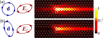
Figure 1: (a) Simulation of a circular dipole source located at a point of elliptical polarisation in a photonic crystal waveguide. Light is emitted in both directions but the forwards direction is preferred. (b) Replacing the circular dipole source with the depicted elliptical one results in unidirectional emission as this dipole is orthogonal to the polarisation of the backward mode.

However, there will always be a dipole orthogonal to the polarisation of the backwards mode, $\mathbf{d}_{\perp}^{*}\cdot\mathbf{E}_{b}=0$, so that there is no emission backward. For any polarisation except linear, this dipole will be non-orthogonal to the polarisation of the forwards mode, $\mathbf{d}_{\perp}^{*}\cdot\mathbf{E}_{f}\neq 0$ resulting in emission in only the forward direction Rodríguez-Fortuño et al. (2013); Petersen et al. (2014); Perea-Puente and Rodríguez-Fortuño (2021); Picardi et al. (2018); Mechelen and Jacob (2016); no et al. (2014). An example is shown in Fig.1(b). By setting the dipole’s long axis orthogonal to the long axis of the polarisation the linear components have been cancelled, leaving only a circular-like effect (unidirectional emission). This demonstrates that the directional contrast is not in general limited by the degree of circular polarisation, and can be unity with any polarisation (except exactly linear) given the correct emission dipole.

The chirality can be measured using the directional contrast, the difference between the power radiated forwards and backwards divided by the sum of the two, $D=(|\mathbf{d}^{*}\cdot\mathbf{E}_{f}|^{2}-|\mathbf{d}^{*}\cdot\mathbf{E}_{b}|^{2})/(|\mathbf{d}^{*}\cdot\mathbf{E}_{f}|^{2}+|\mathbf{d}^{*}\cdot\mathbf{E}_{b}|^{2})$. For a circular dipole it takes the same value as the (normalised) Stokes parameter describing the degree of circular polarisation $D=S_{3}=2\,\text{Im}(E_{x}^{*}E_{y})/|\mathbf{E}|^{2}$ Lang et al. (2015). In figure 2(a) we assess a typical photonic crystal waveguide mode with wavevector $k_{x}=0.395(2\pi/a)$, for lattice constant $a$ Johnson and Joannopoulos (2001). The hole radii/slab height are $r=0.3a$ and $h=0.6a$ respectively as in Lang et al. (2017). The polarisation varies spatially, such that a circular dipole is strongly directional ($|D|\geq 0.9$) over small areas as indicated by the darkest shading. However, for each location (except on lines of zero area) there is a dipole that is unidirectional. A specific elliptical dipole is shown, which is “half circular” in the sense that $S_{3}=S_{1}=1/\sqrt{2}$, with $S_{1}=(|E_{y}|^{2}-|E_{x}|^{2})/|\mathbf{E}|^{2}$ the Stokes parameter for rectilinear polarisation. It is noticeable that with this dipole a far larger area in the waveguide is useful for unidirectional coupling. Finally we mark the areas for which there exists a dipole that is at least half-circular ($S_{3}\geq 1/\sqrt{2}$) which has $|D|\geq 0.9$. This area is $\sim 30$ times larger than that in which $|D|>0.9$ occurs with a circular dipole. Had we considered $|D|>0.95$ the increase would instead be $\sim\times 45$ will be the supplementary information .

The two crucial parameters for a chiral light-matter interface are the directional contrast and the fraction of light that is emitted into the waveguide, known as the Beta factor Scarpelli et al. (2019). We have shown that one can recover high directional contrast with elliptical polarisation. However, it is important to assess how this will effect the Beta factor, which is largely determined by the coupling rate between the MS and waveguide ($\propto|\mathbf{d}^{*}\cdot\mathbf{E}_{f}|^{2}+|\mathbf{d}^{*}\cdot\mathbf{E}_{b}|^{2}$). Typically a higher electric field intensity will be possible away from a C point Scarpelli et al. (2019); Lang et al. (2016). However, away from the C point the polarisations of the forwards and backwards modes are non-orthogonal, and thus the dipole orthogonal to the backward mode has poorer overlap with the forward mode. Accounting for both effects the overall unidirectional coupling strength varies as $S_{3}^{2}(\mathbf{r})|\mathbf{E}(\mathbf{r})|^{2}|\mathbf{d}|^{2}$.

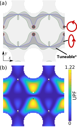
Figure 2: (a) Positions where different types of dipole source have $|D|\geq 0.9$ in a waveguide mode. Darkest - circular dipole; next darkest - (fixed) elliptical dipole as shown ($S_{1}=\sqrt{1/2}$). Second palest - Variable elliptical dipole, tuned for maximum $|D|$ subject to $S_{3}\geq 1/\sqrt{2}$ (marked tuneable^∗). Large white circles - air holes. (b) Unidirectional Purcell factor. White/black dots are right/left polarised C points where unidrectional emission occurs for circular dipoles. In contrast, all locations with UPF$\neq 0$ enable unidirectional coupling with suitably elliptical dipoles.

In Fig.2(b) we explore the impact of these competing effects. At each location the unidirectional coupling rate after the dipole has been adjusted for the new location is plotted. The rate is normalised to the emission rate in bulk GaAs (refractive index $n=3.45$) to give a Purcell factor; $P(\mathbf{r})=S_{3}^{2}(\mathbf{r})|\mathbf{E}(\mathbf{r})|^{2}\,\,(3/8\pi v_{g}f^{2}n)$ with $f$ the mode frequency and $v_{g}$ the group velocity, expressed in units of $c/a$ and $c$ respectively Manga Rao and Hughes (2007). In Fig.2 $f=0.262(c/a)$ and $v_{g}=0.03c$.

Coupling matching that at a C point is achieved over a significant area, indeed coupling is not maximised at the C points: It is over 50% higher at other locations where increased field intensity has more than compensated for the reduction in overlap between the dipole and the forwards mode. Comparison with part (a) of the figure further shows that the elliptical dipole not only couples unidirectionally in more places, but also does so in places with stronger coupling.

Scattering - As well as emission, unidirectional coupling also has important consequences for the scattering of photons from the MS. To model scattering we assume that initially the MS is in its ground state and the forwards waveguide mode is populated with a single photon. The scattering amplitudes with which the MS (re)-directs the incident photon are then calculated using a method based on the photonic Green’s function. Our aim is to avoid input/output theory which can cause confusion in chiral systems The calculation involves a number of steps, summarised here and detailed in the supplementary information will be the supplementary information .

The interaction between the MS and light is included perturbatively. The probability amplitude in the state $\ket{k}$, $\gamma_{k}(t)$ at time $t$ is given by $\gamma_{k}(t)=\sum_{l=0}^{\infty}\gamma_{k}^{(l)}(t)$, where $\gamma_{k}^{(0)}$ is defined by the initial condition and all subsequent orders are calculated from the previous according to:

$$\gamma_{k}^{(z+1)}(T)=\int\limits^{T}\sum_{m}\bra{k}\hat{H}\ket{m}\frac{\gamma_{m}^{(z)}(t)}{\text{i}\hbar}e^{\text{i}(E_{k}-E_{m})t/\hbar}dt,$$ (1)

with the sum over all states of the system, $E_{m}$ the unperturbed energy of the state $\ket{m}$, and $H$ the interaction Hamiltonian Grynberg et al. (2010).

Adopting the long photon limit (a single frequency photon), we can expand the integration range to $\pm\infty$. Further the Hamiltonian is assumed to turn off slowly as one approaches $|t|\rightarrow\infty$ as in Shen and Fan (2007). Together these assumptions result in each even perturbation order being given by the previous even order times a fixed multiplier, allowing all orders to be collected using a geometric series.

The Hamiltonian for light coupling to a two level system with a single optical transition (in the rotating wave approximation) is given by: $\hat{H}=-\text{i}\hat{\sigma}^{+}\hat{l}+\text{h.c.}$ with Scheel et al. (1999); Ge et al. (2013),

$$\hat{l}=\mathbf{d}\iint\textbf{G}(\mathbf{r},\mathbf{r}^{\prime},\omega^{\prime})\sqrt{\frac{\hbar\text{Im}[\epsilon(\mathbf{r}^{\prime},\omega^{\prime})]}{\epsilon_{0}\pi}}\mathbf{\hat{f}}(\mathbf{r}^{\prime},\omega^{\prime})d^{3}\mathbf{r}^{\prime}d\omega^{\prime}\,,$$ (2)

where $\textbf{G}(\mathbf{r},\mathbf{r}^{\prime},\omega^{\prime})$ is the tensor electromagnetic Green’s function connecting locations $\mathbf{r}$ and $\mathbf{r}^{\prime}$ at frequency $\omega^{\prime}$. The raising operator of the two-level system is $\hat{\sigma}^{+}$. The dielectric profile is given by $\epsilon$ and $\mathbf{\hat{f}}(\mathbf{r}^{\prime},\omega^{\prime})$ is the annihilation operator of a bosonic excitation in the dielectric material and its associated electromagnetic field Knoll et al. (2000).

$\hat{H}$ is inserted into the perturbation model and standard Green’s function identities Gruner and Welsch (1996); Ge et al. (2013); Van Vlack et al. (2012), are exploited to simplify the spatial and frequency integrals. Finally an integration over a small frequency window is introduced, representing the resolution of a detector. This is necessary to correctly normalise the density of states.

The result of this calculation is the following equations for the (complex) transmission and reflection amplitudes (the probability amplitudes with which the photon will be found in the forwards/backwards modes in the long-time limit):

$$t=1-\frac{\mathbf{d}\cdot\mathbf{E}_{f}^{*}(\mathbf{r})\,\,\mathbf{d}^{*}\cdot\mathbf{E}_{f}(\mathbf{r})}{D}\,,$$ (3)

$$r=-\frac{\mathbf{d}\cdot\mathbf{E}_{b}^{*}(\mathbf{r})\,\,\mathbf{d}^{*}\cdot\mathbf{E}_{f}(\mathbf{r})}{D}\,,$$ (4)

$$\begin{split}D=&\frac{1}{2}\left[|\mathbf{d}^{*}\cdot\mathbf{E}_{f}(\mathbf{r})|^{2}+|\mathbf{d}^{*}\cdot\mathbf{E}_{b}(\mathbf{r})|^{2}\right]\\ &+\zeta\left(\mathbf{d}\cdot\mathbf{G}_{\text{Loss}}\cdot\mathbf{d}^{*}+\text{i}\hbar\epsilon_{0}\Delta\right)\,,\end{split}$$ (5)

where $\mathbf{G}_{\text{Loss}}$ represents the Green’s function of the loss mode(s) (with both spatial dependencies set to $\mathbf{r}$) and $\Delta$ the detuning between the photon and the transition frequency. The $\mathbf{E}$ terms are the electric fields of Bloch modes normalised as $\int\epsilon(\mathbf{r})|\mathbf{E}(\mathbf{r})|^{2}=1$ with the integration over a single unit cell of the waveguide (or over the cross section for a translationally invariant waveguide like a fibre). In a translationally periodic (invariant) waveguide $\zeta=\frac{2v_{g}}{a\omega}$ ($\zeta=\frac{2v_{g}}{\omega}$) with $\omega$ the transition angular frequency.

The derivation can be extended to systems with more than two levels and multiple dipole-allowed transitions. Consider a four level system with only two allowed transitions, one connecting $\ket{g_{1}}$ to $\ket{e_{1}}$, and the other $\ket{g_{2}}$ to $\ket{e_{2}}$, an arrangement we denote as II by analogy to the well known $\Lambda$ and $V$ systems Shomroni et al. (2014)(Fig.4). Here there are two dipoles, $\mathbf{d}_{1}$, $\mathbf{d}_{2}$, one for each transition. Similarly there are two detunings. If the system is initially in one of the ground states then equations (3, 4) apply, using the detuning and dipole associated with the transition available to the initial ground state. An initial superposition of ground states simply implies a superposition of reflection/transmission coefficients:

$$\begin{split}\large(\alpha\ket{g_{1}}+\beta\ket{g_{2}}\large)\ket{1_{f}}&\rightarrow\\ \alpha\ket{g_{1}}(t_{1}\ket{1_{f}}+r_{1}\ket{1_{b}})&+\beta\ket{g_{2}}(t_{2}\ket{1_{f}}+r_{2}\ket{1_{b}}),\end{split}$$ (6)

where $r_{n}$, $t_{n}$ are the reflection/transmission coefficients calculated from equations (3, 4) using the dipole and detuning of the $n^{\text{th}}$ transition. This is the underlying mechanism behind some proposals to entangle the emitter with a photon Young et al. (2015).

Scattering calculations for systems where a single ground/excited state has multiple allowed transitions, such as V and $\Lambda$ arrangements require a more complicated treatment Hughes and Agarwal (2017); Lang (2017). However, the dot-product rules that determine directionality are unchanged.

Chiral interactions at C points are characterised not just by an excited MS radiating light in only one direction, but also by a single-photon transmission coefficient that approaches $-1$ for low loss - i.e. transmission of the incident photon with a phase shift of $\pi$. This phase shift is exploited in several proposals for quantum information circuits Young et al. (2015); Mahmoodian et al. (2016); Söllner et al. (2015); Li et al. (2018). However this effect is not fundamentally associated with either circular dipoles or polarisations, but emerges whenever the interaction between the MS and waveguide is unidirectional.

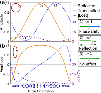
Figure 3: Single photon reflection (solid) and transmission (dotted) coefficients for a two level MS as a function of the dipole moment. Curves are calculated using equations (3, 4) with $\Delta$ = 0, $|\mathbf{E}|=|\mathbf{d}|=1$ and $\zeta\mathbf{d}\cdot\mathbf{G}_{\text{Loss}}\cdot\mathbf{d}^{*}=0.01$. Dashed: lost intensity, right axis. In (a) the polarisation is circular so that a dipole matching the helicity of the light phase shifts a passing photon (1), while a dipole of opposite helicity transmits the photon with no phase shift (3). Linear dipoles reflect the photon (2). In (b) with elliptical polarisation note that there are still dipoles that transmit a photon with or without a phase shift.

This is shown in Fig.3 where the reflection and transmission coefficients from equations (3, 4) are plotted. In parts (a) and (b) the local polarisation is given by $\mathbf{E}_{f}=1/\sqrt{2}\begin{pmatrix}1&\text{i}\end{pmatrix}$ and $\mathbf{E}_{f}=1/\sqrt{10}\begin{pmatrix}1&3\text{i}\end{pmatrix}$ (an arbitrary choice) respectively while along the $x$ axis the dipole is varied as $\mathbf{d}=\begin{pmatrix}\cos\theta&\text{i}\sin\theta\end{pmatrix}$ with $\theta$ running from $0$ to $\pi$. A phase-shift ($t\approx-1$) occurs when $\mathbf{d}^{*}\cdot\mathbf{E}_{b}=0$, a consequence of the fact that in this configuration the forwards/backwards emission rates are identical to those with a circular dipole at a C point, indeed there is no special feature that separates chirality with circles from that with ellipses.

More generally, many interesting effects have been predicted in theoretical frameworks where particular forward/backward emission rates are assumed Mahmoodian et al. (2016); Li et al. (2018); Ramos et al. (2014); Söllner et al. (2015); Shomroni et al. (2014); Pichler et al. (2015); Mirza and Schotland (2016), rather than specifying the dipoles/polarisations that determine these rates. The predictions of these works apply to all polarisation/dipole combinations that produce directionality.

Comparing the points with transmission approaching $-1$ of parts (a) and (b) of Fig.3 notice the losses are higher in (b). Here the poorer dot product between the dipole and the forwards mode, combined with our assumption that $|\mathbf{E}|$ is unchanged between parts (a, b) has led to a reduced Beta factor. However, as discussed previously $|\mathbf{E}|$ can be much higher at elliptical points and this will often more than compensate for the lower overlap. As seen in Fig.2 the choices that maximise coupling (and consequently minimise this loss) are ellipses.

Some proposals require a MS with more than two levels. We consider two specific schemes, both with potential applications in quantum information. First that of Young et al. (2015), which makes use of charged QDs, described as a II-like four-level system. Second Shomroni et al. (2014), with Caesium atoms described with three levels in a $\Lambda$-like configuration. In both cases there are two relevant optical transitions and in both ideally one transition couples only to the forwards direction, while the other couples only backwards, depicted in Fig.4. As seen in part (b) of the figure the ideal pair consists of two elliptical dipoles, identical in all respects except for helicity (the arrowhead direction) which is opposite between them. That is, ideally $\mathbf{d}_{1}=\mathbf{d}_{2}^{*}$ and $\mathbf{d}_{1}^{*}\cdot\mathbf{E}_{b}=0$.

The non-orthogonality of the two dipoles in fig.4(b) is no impediment to the quantum information proposals, as the orthogonality of dipoles in real space does not equate to orthogonality of quantum states in Hilbert space will be the supplementary information .

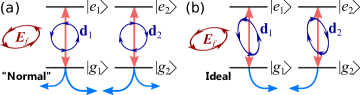
Figure 4: (a) Four level system with two transitions with opposite circular dipole moments. Each transition interacts with both waveguide directions (blue arrows). (b) The dipole arrangement such that each interacts with only a single waveguide direction. For this polarisation (b) represents the ideal situation for the protocols discussed in the text, in contrast to (a).

Dipole engineering - Finally we propose illustrative schemes to achieve the necessary dipole engineering in either an atomic or a QD system, focusing on proposals that call for two transitions which are unidirectional in opposite directions Shomroni et al. (2014); Young et al. (2015).

Atoms - Given a system with a circular transition dipole one can imagine rotating the system in 3D space so that the projection of the circular dipole onto the 2D plane spanned by the waveguide mode’s electric field resembles the desired ellipse. If provided a system with oppositely circular transitions rotating it to make one transition couple only to the forward mode will result in the other coupling only to the backward mode. With atoms in vacuum Mitsch et al. (2014); Shomroni et al. (2014), it is the external magnetic field that defines the quantisation axis, so that the relevant transitions have circular dipole moments in the plane orthogonal to the magnetic field direction Scheel et al. (2015); Grynberg et al. (2010). Consequently tilting the applied magnetic field will have the desired effect.

QDs - In QDs there will be in-plane strain, which leads to mixing between the heavy and light holes. The dipole associated with the recombination of an electron with a light-hole has the opposite sense of circular polarisation to that for recombination with a heavy hole. As a result recombination with the mixed holes in the QD is related to an elliptical dipole Koudinov et al. (2004), typically with 1%-20% degree of linear polarization ($\sqrt{1-S_{3}^{2}}=0.01\text{--}0.2$). The dipoles of the two QD transitions are stretched along the same axis, providing the ideal configuration. The degree of linear polarisation in these dipoles can be enhanced to up to 40% by annealing Harbord et al. (2013), and can be tuned $\pm$20% with application of strain Plumhof et al. (2013). Two strategies emerge: first, annealing allows the creation of QD-waveguide samples where the (randomly located) QDs are more likely to have a high directionality and stronger waveguide coupling; second, it may be possible to exploit strain-tuning techniques to modify the dipole of a particular QD in situ to maximise the directionality.

Conclusion - We propose the engineering of elliptical dipoles in quantum emitters as an approach to building chiral interfaces. These strategies offer the two-fold advantage of making far more of the space within a waveguide useful for directional interactions while simultaneously enabling a higher photon collection efficiency.

Advanced proposals call for a system with two transitions, each unidirectional but in opposite directions. This requires that the opposite circular dipoles are replaced with ellipses stretched along a shared axis. We have outlined methods to achieve these arrangements in both atomic and QD systems.

In summary, circular polarisations and transition dipoles are not necessary for chiral interactions, furthermore they are typically not the most efficient choices.

Additional references Loudon (1973); Chen et al. (2011); Yao et al. (2010) are used in the Supplemental information.

Acknowledgements - We gratefully acknowledge EPSRC funding through the projects 1D QED (EP/N003381/1), SPIN SPACE (EP/M024156/1) and BL’s studentship (DTA-1407622). This work was also supported by Leverhulme Trust Research Project Grant No. RPG-2018-213. We thank Joseph Lennon for help with data access issues.

See pages 1 of Supplementary_Info_new.pdf See pages 2 of Supplementary_Info_new.pdf See pages 3 of Supplementary_Info_new.pdf See pages 4 of Supplementary_Info_new.pdf See pages 5 of Supplementary_Info_new.pdf See pages 6 of Supplementary_Info_new.pdf See pages 7 of Supplementary_Info_new.pdf See pages 8 of Supplementary_Info_new.pdf

References

- Turchette et al. (1995) Q. Turchette, R. Thompson, and H. Kimble, Applied Physics B, Supplement 60, S1 (1995).
- Auffèves-Garnier et al. (2007) A. Auffèves-Garnier, C. Simon, J.-M. Gérard, and J.-P. Poizat, Phys. Rev. A 75, 053823 (2007).
- Waks and Vuckovic (2006) E. Waks and J. Vuckovic, Phys. Rev. Lett. 96, 153601 (2006).
- Aiello et al. (2015) A. Aiello, P. Banzer, M. Neugebauer, and G. Leuchs, Nature Photonics 9, 789 (2015).
- Coles et al. (2016) R. J. Coles, D. M. Price, J. E. Dixon, B. Royall, E. Clarke, P. Kok, M. S. Skolnick, A. M. Fox, and M. N. Makhonin, Nature Communications 7 (2016), 10.1038/ncomms11183.
- Young et al. (2015) A. B. Young, A. C. T. Thijssen, D. M. Beggs, P. Androvitsaneas, L. Kuipers, J. G. Rarity, S. Hughes, and R. Oulton, Phys. Rev. Lett. 115, 153901 (2015).
- Bliokh et al. (2015) K. Y. Bliokh, D. Smirnova, and F. Nori, Science 348, 1448 (2015).
- Rodríguez-Fortuño et al. (2013) F. J. Rodríguez-Fortuño, G. Marino, P. Ginzburg, D. O’Connor, A. Martínez, G. A. Wurtz, and A. V. Zayats, Science 340, 328 (2013).
- Jones et al. (2020) R. Jones, G. Buonaiuto, B. Lang, I. Lesanovsky, and B. Olmos, Phys. Rev. Lett. 124, 093601 (2020).
- Lodahl et al. (2017) P. Lodahl, S. Mahmoodian, S. Stobbe, A. Rauschenbeutel, P. Schneeweiss, J. Volz, H. Pichler, and P. Zoller, Nature 541, 473 (2017).
- Luxmoore et al. (2013) I. J. Luxmoore, N. A. Wasley, A. J. Ramsay, A. C. T. Thijssen, R. Oulton, M. Hugues, S. Kasture, V. G. Achanta, A. M. Fox, and M. S. Skolnick, Phys. Rev. Lett. 110, 037402 (2013).
- Petersen et al. (2014) J. Petersen, J. Volz, and A. Rauschenbeutel, Science 346, 67 (2014).
- Burresi et al. (2009) M. Burresi, R. J. P. Engelen, A. Opheij, D. van Oosten, D. Mori, T. Baba, and L. Kuipers, Phys. Rev. Lett. 102, 033902 (2009).
- Söllner et al. (2015) I. Söllner, S. Mahmoodian, S. L. Hansen, L. Midolo, A. Javadi, G. Kiršanskė, T. Pregnolato, H. El-Ella, E. H. Lee, J. D. Song, S. Stobbe, and P. Lodahl, Nature Nanotechnology 10, 775 (2015).
- Perea-Puente and Rodríguez-Fortuño (2021) S. Perea-Puente and F. J. Rodríguez-Fortuño, Phys. Rev. B 104, 085417 (2021).
- Picardi et al. (2018) M. F. Picardi, A. V. Zayats, and F. J. Rodríguez-Fortuño, Phys. Rev. Lett. 120, 117402 (2018).
- Mechelen and Jacob (2016) T. V. Mechelen and Z. Jacob, Optica 3, 118 (2016).
- no et al. (2014) F. J. R.-F. no, D. Puerto, A. Griol, L. Bellieres, J. Martí, and A. Martínez, Opt. Lett. 39, 1394 (2014).
- (19) T. T. will be the supplementary information, .
- Oskooi. et al. (2010) A. F. Oskooi., D. Roundy, M. Ibanescu, P. B. Mihai, J. D. Joannopoulos, and S. G. Johnson, Computer Physics Communications 181, 687 (2010).
- Note (1) Simulation parameters. Structure as fig.2. Source frequency . Source position relative to origin centred on waveguide between two holes. In (a): , (b): .
- Lang et al. (2015) B. Lang, D. M. Beggs, A. B. Young, J. G. Rarity, and R. Oulton, Phys. Rev. A 92, 063819 (2015).
- Johnson and Joannopoulos (2001) S. G. Johnson and J. D. Joannopoulos, Opt. Express 8, 173 (2001).
- Lang et al. (2017) B. Lang, R. Oulton, and D. M. Beggs, J. Opt. 19, 045001 (2017).
- Scarpelli et al. (2019) L. Scarpelli, B. Lang, F. Masia, D. M. Beggs, E. A. Muljarov, A. B. Young, R. Oulton, M. Kamp, S. Höfling, C. Schneider, and W. Langbein, Phys. Rev. B 100, 035311 (2019).
- Lang et al. (2016) B. Lang, D. M. Beggs, and R. Oulton, Phil. Trans. R. Soc. A 374 (2016), 10.1098/rsta.2015.0263.
- Manga Rao and Hughes (2007) V. S. C. Manga Rao and S. Hughes, Phys. Rev. B 75, 205437 (2007).
- Note (2) For example Shen et al. (2011) and Söllner et al. (2015) draw differing conclusions using input/output theory.
- Grynberg et al. (2010) G. Grynberg, A. Aspect, and C. Fabre, Introduction to Quantum Optics: From the Semi-classical Approach to Quantized Light (Cambridge University Press, 2010).
- Shen and Fan (2007) J.-T. Shen and S. Fan, Phys. Rev. A 76, 062709 (2007).
- Scheel et al. (1999) S. Scheel, L. Knöll, and D.-G. Welsch, Phys. Rev. A 60, 4094 (1999).
- Ge et al. (2013) R.-C. Ge, C. Van Vlack, P. Yao, J. F. Young, and S. Hughes, Phys. Rev. B 87, 205425 (2013).
- Knoll et al. (2000) L. Knoll, S. Scheel, and D.-G. Welsch, arXiv:quant-ph/0006121 (2000).
- Gruner and Welsch (1996) T. Gruner and D.-G. Welsch, Phys. Rev. A 53, 1818 (1996).
- Van Vlack et al. (2012) C. Van Vlack, P. T. Kristensen, and S. Hughes, Phys. Rev. B 85, 075303 (2012).
- Shomroni et al. (2014) I. Shomroni, S. Rosenblum, Y. Lovsky, O. Bechler, G. Guendelman, and B. Dayan, Science 345, 903 (2014).
- Hughes and Agarwal (2017) S. Hughes and G. S. Agarwal, Phys. Rev. Lett. 118, 063601 (2017).
- Lang (2017) B. Lang, Thesis (2017).
- Mahmoodian et al. (2016) S. Mahmoodian, P. Lodahl, and A. S. Sørensen, Phys. Rev. Lett. 117, 240501 (2016).
- Li et al. (2018) T. Li, A. Miranowicz, X. Hu, K. Xia, and F. Nori, Phys. Rev. A 97, 062318 (2018).
- Ramos et al. (2014) T. Ramos, H. Pichler, A. J. Daley, and P. Zoller, Phys. Rev. Lett. 113, 237203 (2014).
- Pichler et al. (2015) H. Pichler, T. Ramos, A. J. Daley, and P. Zoller, Phys. Rev. A 91, 042116 (2015).
- Mirza and Schotland (2016) I. M. Mirza and J. C. Schotland, Phys. Rev. A 94, 012302 (2016).
- Mitsch et al. (2014) R. Mitsch, C. Sayrin, B. Albrecht, P. Schneeweiss, and A. Rauschenbeutel, Nature Communications 5 (2014).
- Scheel et al. (2015) S. Scheel, S. Y. Buhmann, C. Clausen, and P. Schneeweiss, Phys. Rev. A 92, 043819 (2015).
- Koudinov et al. (2004) A. V. Koudinov, I. A. Akimov, Y. G. Kusrayev, and F. Henneberger, Phys. Rev. B 70, 241305 (R) (2004).
- Harbord et al. (2013) E. Harbord, Y. Ota, Y. Igarashi, M. Shirane, N. Kumagai, S. Ohkouchi, S. Iwamoto, S. Yorozu, and Y. Arakawa, Japanese Journal of Applied Physics 52, 125001 (2013).
- Plumhof et al. (2013) J. D. Plumhof, R. Trotta, V. Křápek, E. Zallo, P. Atkinson, S. Kumar, A. Rastelli, and O. G. Schmidt, Phys. Rev. B 87, 075311 (2013).
- Loudon (1973) R. Loudon, The Quantum Theory of Light (OUP Oxford, 1973).
- Chen et al. (2011) Y. Chen, M. Wubs, J. Mørk, and A. F. Koenderink, New J. Phys 13, 103010 (2011).
- Yao et al. (2010) P. Yao, V. Manga Rao, and S. Hughes, Laser & Photonics Reviews 4, 499 (2010).
- Shen et al. (2011) Y. Shen, M. Bradford, and J.-T. Shen, Phys. Rev. Lett. 107, 173902 (2011).