Deep Bayesian Estimation for Dynamic Treatment
Regimes with a Long Follow-up Time

Abstract

Causal effect estimation for dynamic treatment regimes (DTRs) contributes to sequential decision making. However, censoring and time-dependent confounding under DTRs are challenging as the amount of observational data declines over time due to a reducing sample size but the feature dimension increases over time. Long-term follow-up compounds these challenges. Another challenge is the highly complex relationships between confounders, treatments, and outcomes, which causes the traditional and commonly used linear methods to fail. We combine outcome regression models with treatment models for high dimensional features using uncensored subjects that are small in sample size and we fit deep Bayesian models for outcome regression models to reveal the complex relationships between confounders, treatments, and outcomes. Also, the developed deep Bayesian models can model uncertainty and output the prediction variance which is essential for the safety-aware applications, such as self-driving cars and medical treatment design. The experimental results on medical simulations of HIV treatment show the ability of the proposed method to obtain stable and accurate dynamic causal effect estimation from observational data, especially with long-term follow-up. Our technique provides practical guidance for sequential decision making, and policy-making.

I Introduction

Many real-world situations require a series of decisions, so a rule is needed (also referred to as a dynamic treatment regime (DTR), plan or policy) to assist making decisions at each step. For example, a doctor usually needs to design a series of treatments in order to cure patients. The treatment often varies over time, and the treatment assignment at each time point depends on the patient’s history, which includes the patient’s past treatments, the observed static or dynamic covariates that denote the patient’s characteristics, and the past measured outcomes of the patient’s disease. Estimating the causal effect of specific dynamic treatment regimes over time (also known as dynamic causal effect estimation) benefits decision makers when facing sequential decision-making problems. For example, estimating the effect of a series of treatments given by a doctor can apparently guide the real selection of correct treatments for patients. Although the gold standard for dynamic causal effect estimation is randomized controlled experiments, it is often either unethical, technically impossible, or too costly to implement [1]. For example, for patients diagnosed with the human immunodeficiency virus (HIV), it is unethical to pause their treatment for the sake of a controlled experiment. Hence, causal effect estimation is often conducted using uncontrolled observational data, which typically includes observed confounders, treatments, and outcomes.

The challenges associated with estimating the causal effect of DTR are censoring and time-dependent confounding. For example, the patients may quit the treatments due to dead over time and then the outcome values of these patients are unknown (censoring). Furthermore, the features and outcomes of former time steps also affect current treatments and current outcomes, so this increases the features of current time point (time-dependent confounding). A longer follow-up makes the challenges even more difficult. Another challenge is to address the highly complex relationships between confounders, treatments, and outcomes, which causes the traditional and commonly used linear methods to fail.

A motivating example is a HIV treatment research study with a focus on children’s growth outcomes, measured by height-for-age z-scores (HAZ). The subjects of the study are HIV-positive children who were diagnosed with AIDS, before the commencement of the study. The treatment is antiretroviral (ART) which is a dynamic binary treatment. The study is to evaluate the effect of different treatment regimes applied to HAZ. The research took a couple of months to observe the outcomes at a time point of interest. A child may be censored during the study, where they may cease to follow the study during the treatment process. Censoring leads to a reduction in the number of subjects at each time point in the HIV treatment research study, since not all the children may survive the study after several months. ART may also bring drug-related toxicities, so a judgement needs to be made as to whether to use ART or not by the measurements of a child’s cluster of differentiation 4 count (CD4 count), CD4%, and weight for age z-score (WAZ). These measurements also serve as a disease progression measure for the child. The CD4 count, CD4%, and WAZ are affected by prior treatments and also influence treatments (ART initiation) and the outcomes (HAZ) at a later stage. Thus, CD4 count, CD4%, and WAZ are time-dependent confounders.

Existing methods can be roughly categorised into three groups. The first group requires the treatment models to fit for both the treatment and censoring mechanisms (these mechanisms model the treatment assignment process and the missing data mechanism), such as the inverse probability of treatment weighting (IPTW) [2]. However, the cumulative inverse probability weights may be small due to the censoring problem, which leads to a near positivity violation (this violation makes it difficult to trust the estimates provided by the methods). The second group fits the outcome regression models (these models are to estimate the relationships between the outcome and the other variables), such as the sequential g-formula (seq-gformula) [3]. However, the outcome regression models may introduce bias into seq-gformula . The last group is a doubly robust method (LTMLE) [4, 5], which combines the iterated outcome regressions and the inverse probability weights estimated by treatment models. However, it suffers from the censoring problem because the observational data reduces in the long-term which in turn decreases the modeling performance, especially with long-term follow-up.

In this paper, we propose a two-step model to combine the iterated outcome regressions and the inverse probability weights, where the uncensored subjects until the time point of interest are all used. Hence our model improves the target parameter using potentially more subjects than LTMLE. LTMLE improves the target parameter using the uncensored subjects following the treatment regime of interest. It is for this reason that it is problematic to fit a limited number of subjects following the treatment regime of interest for common models in the long-term follow-up study. As our model uses a larger number of subjects in the estimation improvement, it may achieve better performance and stability. To capture the complex relationships between confounders, treatments, and outcomes in the DTRs, we apply a deep Bayesian method to the outcome regression models. The deep Bayesian method has a powerful capability to reveal complex hidden relationships using subjects of a small sample size. The experiments show that our method demonstrates the better performance and stability compared with other popular methods.

The three contributions of our study are summarised as follows:

• Our method is able to use all the uncensored data samples which cannot be fully used by other methods like LTMLE, so our method is able to achieve a more stable performance.

• A deep Bayesian method is applied to the iterated outcome regression models. A deep Bayesian method has a strong ability to capture the complex hidden relationships between the confounders, the treatments, and the outcomes in a small-scale dataset with high dimensions.

• The deep Bayesian method is able to capture the uncertainty for the causal prediction of every subject. Such uncertainty modeling is essential for the safety-aware applications, like self-driving cars and medical treatment design.

The remainder of this paper is organized as follows. Section II discusses the related work. Section III describes the problem setting and a deep Bayesian method. We introduce our deep Bayesian estimation for dynamic causal effect in Section IV. Section V describes the experiments with a detailed analysis of our method and its performance compared with other methods. Finally, Section VI concludes our study and discusses future work.

II Related Work

In the majority of previous work, learning the causal structure [6, 7, 8, 9, 10, 11] or conducting causal inference from observational data in the static setting (a single time point) [12, 13, 14, 15, 16, 17] have been proposed. These methods cannot be applied to dynamic causal effect estimation [18, 19] directly. A few methods focus on the counterfactual prediction of outcomes for future treatments [20, 18, 21, 22]. Counterfactual prediction methods aim to estimate the causal effect of the following future treatment, which is different from our problem setting.

Another body of work focuses on selecting optimal DTRs [23, 21]. G-estimation [24, 25] has been proposed for optimal DTRs in the statistical and biomedical literature. G-estimation builds a parametric or semi-parametric model to estimate the expected outcome. Two common machine learning approaches, Q-learning [26] and A-learning [27], are applied to estimate DTRs. Q-learning is based on regression models for the outcomes given in the patient information and is implemented via a recursive fitting procedure. A-learning builds regret functions that measure the loss incurred by not following the optimal DTR. It is easy for the Q-functions of Q-learning and the regret functions of A-learning to fit poorly in high dimensional data.

Finally, we discuss the methods proposed to estimate the dynamic causal effect. The methods proposed to evaluate DTRs from observational data include the inverse probability of treatment weighting (IPTW) [2], the marginal structural model (MSM) [28, 19], sequential g-formula (seq-gformula) [3], and the doubly robust method (LTMLE) [4, 5]. IPTW estimates dynamic causal effect using the data from a pseudo-population created by inverse probability weighting. The misspecified parametric models used for the treatment models will lead to inaccurate estimation. MSM fits a model that combines information from many treatment regimes to estimate the dynamic causal effect. However, MSM may result in bias introduced by the regression model for the potential outcome and bias introduced by treatment models. Sequential g-formula uses the iterated conditional expectation to estimate the average causal effect. The performance of sequential g-formula relies on the accuracy of the outcome regression models. LTMLE calculates the cumulative inverse probabilities by the treatment models on the uncensored subjects who follow the treatment regime of interest. Then it fits the outcome regression models and uses the cumulative inverse probabilities calculated to improve the target variable. The unstable weights from the treatment models may affect the accuracy of LTMLE.

III Preliminary Knowledge

This section briefly introduces the problem setting using HIV treatment as an example and the deep kernel learning method.

III-A Dynamic Causal Effects

Observational data consists of information about the subjects. In the HIV treatment study, patients are the subjects. For each subject, time-dependent confounders $X_{k}$, treatment $T_{k}$ and outcome $Y_{k}$ are observed at each time point $k$. Given the HIV treatment example, the treatment indicator is whether ART is taken; CD4 variables are affected by previous treatments and influence the latter treatment assignment and outcomes, CD4 variables belong to time-dependent confounders; and HAZ is the outcome. The static confounders $V$ represent each subject’s specific static features, such as patients’ age. We use $L_{k}$ to describe the union of static confounders $V$ and time-dependent confounders $X_{k}$ at time $k$.

The outcome values are unknown (censored) for some subjects who pass away before follow-up. The censoring variable is represented as $C_{k}$. If a subject does not follow the study, the subject will not attend the following study (if $C_{i}=1$, then $C_{j}=1$, for any time $j>i$). If a subject follows the study at a time point, then the subject has followed the study in all previous time points (if $C_{i}=0$, then $C_{j}=0$, for any time $j<i$). Usually, a few subjects are censored at each time point [4], and fewer subjects would continue to follow the study.

An example of censoring is given in the Table I. At the beginning, all subjects take part in the study. After the first treatment assignment, some subjects do not follow the study. The features of these subjects are “missing” in the following study. As the study continues, an increasing number of subjects fail to follow the study. Thus, fewer subjects are available in the following study, which becomes a problem in the long follow-up study.

TABLE I: An example of censoring. “-” represents a missing value.

Observation	$L_{0}$	$C_{0}$	$Y_{0}$	$T_{0}$	$L_{1}$	$C_{1}$	$Y_{1}$	$T_{1}$	$L_{2}$	$C_{2}$	$Y_{2}$	…	$T_{K}$	$L_{K+1}$	$C_{K+1}$	$Y_{K+1}$
$ob_{0}$	$l_{0}^{0}$	0	$y_{0}^{0}$	$t_{0}^{0}$	$l_{1}^{0}$	1	-	-	-	-	-	…	-	-	-	-
$ob_{1}$	$l_{0}^{1}$	0	$y_{0}^{1}$	$t_{0}^{1}$	$l_{1}^{1}$	0	$y_{1}^{1}$	$t_{1}^{1}$	$l_{2}^{1}$	1	-	…	-	-	-	-
$ob_{2}$	$l_{0}^{2}$	0	$y_{0}^{2}$	$t_{0}^{2}$	$l_{1}^{2}$	0	$y_{1}^{2}$	$t_{1}^{2}$	$l_{2}^{2}$	0	$y_{2}^{2}$	…	$t_{K}^{2}$	$l_{K+1}^{2}$	0	$y_{K+1}^{2}$

To summarise, the observational data can be described as ($L_{0}$, $C_{0}$, $Y_{0}$), ($T_{k-1}$,$L_{k}$, $C_{k}$, $Y_{k}$), for $k$ = 1, …, $K$, and ($T_{K}$, $L_{K+1}$, $C_{K+1}$, $Y_{K+1}$) in $K$+1 time point treatment regimes. All subjects are uncensored at the baseline, which is $C_{0}=0$, and all subjects are untreated before the study, which is represented as $T_{-1}=0$. The $\bar{T}_{k}$ = ($T_{0}$, $T_{1}$, …, $T_{k-1}$,$T_{k}$ ) represents the past treatments until the time $k$. Other symbols with an overbar, such as $\bar{Y}_{k},\bar{L}_{k}$, have similar meanings. The history of covariates at time $k$ is $H_{k}$ = ($\bar{T}_{k-1}$,$\bar{L}_{k}$,$\bar{C}_{k}$,$\bar{Y}_{k}$). For simplicity, the subscript of variables will be omitted unless explicitly needed. Let $Y^{\bar{d}}$ be the potential outcome of the possible treatment rule of interest, $\bar{d}$, and $L^{\bar{d}}$ be the potential covariates of $\bar{d}$. The potential outcome $Y^{\bar{d}}$ is the factual outcome or counterfactual value of the factual outcome.

A treatment regime, also referred to as a strategy, plan, policy, or protocol, is a rule to assign treatment values at each time $k$ of the follow-up. A treatment regime is static if it does not depend on past history $h_{k}$. For example, the treatment regime “always treat” is represented by $\bar{d}_{k}=(1,1,...,1)$, and the treatment regime “never treat” is represented by $\bar{d}_{k}=(0,0,...,0)$. Both two treatment regimes assign a constant value for a treatment, so the assignments do not depend on past history. A dynamic treatment regime depends on the past history $h_{k}$. The treatment assignment at the time point $k$ is $d_{k}=f(h_{k})$. A dynamic treatment regime is a treatment rule $\bar{d}_{k}=(d_{0},...,d_{k})$. The outcome at the time point $k+1$ is affected by the history $h_{k}$, the treatment $t_{k}$, and the observed confounders $l_{k+1}$. The outcome can be described by $y_{k+1}=f(h_{k},t_{k},l_{k+1})$.

Figure 1: The causal graphical model of time-dependent confounding for the time points $k$ and $k+1$. $H$ is the history of past treatments, confounders, and outcomes, $T$ is the treatment, $L$ is the observed confounders, and $Y$ is the outcome.

The causal graph [29] for dynamic treatments is illustrated in Fig. 1. The nodes represent the observed variables. Links connecting the observed quantities are designated by arrows. Links emanating from the observed variables that are causes to the observed variables that are affected by causes. The treatment at time $k$ is influenced by the observed history $H_{k}$. The confounders $L_{k+1}$ and outcome $Y_{k+1}$ at time $k+1$ are influenced by the history $H_{k}$. The confounders $L_{k+1}$ also influence the outcome $Y_{k+1}$.

If all subjects are uncensored, the dynamic causal effect is to estimate the counterfactual mean outcome $E[Y^{\bar{d}_{K}}]$. To adjust the bias introduced by uncensoring in the data, the treatment assignment and uncensoring are considered as a joint treatment [19]. The goal is to estimate the counterfactual mean outcome $E[Y^{\bar{d}_{K},\bar{c}_{K+1}=0}]$. The mean outcome refers to the mean outcome at time $K+1$ that would have been observed if all subjects have received the intended treatment regime $\bar{d}$ and all subjects had been followed-up. The identifiability conditions for the dynamic causal effect need to hold with the joint treatment ($T_{m},C_{m+1}$) at all time $m$, where $m=0,1,...,K$. Note that dynamic causal effect estimation from observational data is possible only with some causal assumptions [19]. Several common causal assumptions are:

• Consistency, that is $Y_{m}^{\bar{d}_{m}}=Y_{m}$ and $\bar{L}_{m}^{\bar{d}_{m}}=\bar{L}_{m}$, if $\bar{T}_{m-1}=\bar{d}_{m-1}$. The consistency assumption means the potential variable equals the observed variable, if the actual treatment is provided.

• Positivity, where $\Pr(T_{m}=\bar{d}_{m}|\bar{L}_{m}=\bar{l}_{m},\bar{Y}_{m}=\bar{y}_{m},\bar{T}_{m-1}=\bar{d}_{m-1})>0$ for all $\bar{d}_{m}$, $\bar{l}_{m}$ and $\bar{y}_{m}$ with $\Pr(\bar{T}_{m-1}=\bar{d}_{m-1},\bar{L}_{m}=\bar{l}_{m},\bar{Y}_{m}=\bar{y}_{m})>0$. The positivity assumption means the subjects have a positive possibility of continuing to receive treatments according to the treatment regime.

• Sequential ignorability, it is $Y_{m}^{\bar{d}_{m}}\mathchoice{\mathrel{\hbox to0.0pt{$\displaystyle\perp$\hss}\mkern 2.0mu{\displaystyle\perp}}}{\mathrel{\hbox to0.0pt{$\textstyle\perp$\hss}\mkern 2.0mu{\textstyle\perp}}}{\mathrel{\hbox to0.0pt{$\scriptstyle\perp$\hss}\mkern 2.0mu{\scriptstyle\perp}}}{\mathrel{\hbox to0.0pt{$\scriptscriptstyle\perp$\hss}\mkern 2.0mu{\scriptscriptstyle\perp}}}T_{m-1}|\bar{L}_{m},\bar{Y}_{m-1},\bar{T}_{m-2}$ for all $\bar{d}_{m}$, $\bar{l}_{m}$ and $\bar{y}_{m-1}$. The symbol $\mathchoice{\mathrel{\hbox to0.0pt{$\displaystyle\perp$\hss}\mkern 2.0mu{\displaystyle\perp}}}{\mathrel{\hbox to0.0pt{$\textstyle\perp$\hss}\mkern 2.0mu{\textstyle\perp}}}{\mathrel{\hbox to0.0pt{$\scriptstyle\perp$\hss}\mkern 2.0mu{\scriptstyle\perp}}}{\mathrel{\hbox to0.0pt{$\scriptscriptstyle\perp$\hss}\mkern 2.0mu{\scriptscriptstyle\perp}}}$ represents statistical independence. The sequential ignorability assumption means all confounders are measured in the data.

The causal assumptions consistency and sequential ignorability cannot be statistically verified [19]. A well-defined treatment regime is a pre-requisite for the consistency assumption. The sequential ignorability assumption requires that the researchers’ expert knowledge is correct.

Based on these assumptions, the counterfactual mean outcome can be estimated from the observational data. Let $L_{k}$ absorb $Y_{k}$ if $k<K+1$ only in the Eq. (1) and Eq. (2). The counterfactual mean outcome $E[Y^{\bar{d}_{K},\bar{c}_{K+1}=0}]$ under the joint treatment ($\bar{d}_{K},\bar{c}_{K+1}=0$) is identifiable through g-formula:

$$\mathbb{E}[Y^{\bar{d}_{K},\bar{c}_{K+1}=0}]=$$ (1)

$$\int_{\bar{l}_{K+1}}\mathbb{E}[Y_{K+1}|\bar{T}_{K}=\bar{d}_{K},C_{K+1}=0,\bar{L}_{K+1}=\bar{l}_{K+1}]$$

$$\hskip 14.22636pt\cdot\prod_{k=0}^{K+1}f(l_{k}|\bar{T}_{k-1}=\bar{d}_{k-1},C_{k-1}=0,\bar{L}_{k-1}=\bar{l}_{k-1})\mathrm{d}\bar{l}_{K+1},$$

with all the subjects remaining uncensored at time $K+1$. When $k=0$, $f(l_{0})$ refers to the marginal distribution of $l_{0}$. After integration with respect to $L$, the iterated conditional expectation estimator [3] can be obtained using the iterative conditional expectation rule, where the equation holds that

$$\mathbb{E}[Y^{\bar{d}_{K},\bar{c}_{K+1}=0}]$$ (2)

$$= \mathbb{E}[\mathbb{E}[\cdots\mathbb{E}[\mathbb{E}[Y_{K+1}|\bar{T}_{K}=\bar{d}_{K},C_{K+1}=0,\bar{L}_{K+1}]$$

$$|\bar{T}_{K-1}=\bar{d}_{K-1},C_{K}=0,\bar{L}_{K}]\cdots|\bar{T}_{0}=d_{0},C_{1}=0,L_{1}|L_{0}]].$$

III-B Deep Kernel Learning

Deep kernel learning (DKL) [30] models are Gaussian process (GP) [31] models that use kernels parameterized by deep neural networks. The definition and the properties of GPs are introduced first. Then, the kernels parameterized by deep neural networks follow.

A Gaussian process can be used to describe a distribution over functions with a continuous domain. The formal definition [31] of GPs is as follows,

Definition 1 (Gaussian Process)

A Gaussian process is a set of random variables, and any finite number of these random variables have a joint Gaussian distribution.

A GP can be determined by its mean function and covariance function. The mean function $m(\mathbf{x})$ and the covariance function $k(\mathbf{x},\mathbf{x^{{}^{\prime}}})$ of a GP $g(\mathbf{x})$ are

$$m(\mathbf{x}) =\mathbb{E}[g(\mathbf{x})],$$ (3)

$$k(\mathbf{x},\mathbf{x^{{}^{\prime}}}) =\mathbb{E}[(g(\mathbf{x})-m(\mathbf{x}))(g(\mathbf{x^{{}^{\prime}}})-m(\mathbf{x^{{}^{\prime}}}))].$$ (4)

The features of the input are represented as $\mathbf{x}$. The $\mathbf{x}$ and $\mathbf{x^{{}^{\prime}}}$ are two input vectors.

Consider observations with additive independent and identically distributed Gaussian noise, that is $y=f(\mathbf{x})+\varepsilon$. Observations can be represented as $\{(\mathbf{x_{i}},y_{i})|i=1,\cdots,n\}$. The GP model for these observations is given by

$$y(\mathbf{x}) =f(\mathbf{x})+\varepsilon,\varepsilon\sim\mathcal{N}(0,\sigma^{2}),$$ (5)

$$f \sim\mathcal{GP}(m,k),$$

$$y \sim\mathcal{GP}(m,k+\sigma^{2}\delta_{ii^{{}^{\prime}}}),$$

where $\delta_{ii^{{}^{\prime}}}$ is the Kronecker’s delta function, that is $\delta_{ii^{{}^{\prime}}}=1$ if and only if $i=i^{{}^{\prime}}$.

The features to evaluate are denoted as $\mathbf{x_{*}}$ and the outputs to evaluate are represented as $f_{*}$. The predictive distribution of the GP—the conditional distribution $f_{*}|X_{*},X,y$ is Gaussian, that is

$$f_{*}|X_{*},X,y\sim\mathcal{N}(\mathbb{E}[f_{*}],\operatorname{cov}(f_{*})),$$ (6)

where $\mathbb{E}[f_{*}]=m(x_{*})+K(X_{*},X)[K(X,X)+\sigma^{2}I]^{-1}(y-m(X))$ and $\operatorname{cov}(f_{*})=K(X_{*},X)-K(X_{*},X)[K(X,X)+\sigma^{2}I]^{-1}K(X_{*},X)$.

The log-likelihood function is used to derive the maximum likelihood estimator. The log likelihood of the outcome $\mathbf{y}$ is:

$$\log p(\mathbf{y}|\gamma,X)\propto-[\mathbf{y}^{T}(K_{\gamma}+\sigma^{2}I)^{-1}\mathbf{y}+\log|K_{\gamma}+\sigma^{2}I|],$$ (7)

where $K_{\gamma}$ denotes kernel function $K(X,X)$ given the parameter $\gamma$.

DKL transforms the inputs of a base kernel with a deep neural network. That is, given a base kernel $k(\mathbf{x}_{i},\mathbf{x}_{j}|\mathbf{\theta})$ with hyperparameters $\mathbf{\theta}$, the inputs $\mathbf{x}$ are transformed as a non–linear mapping $g(\mathbf{x},\mathbf{w})$. The mapping $g(\mathbf{x},\mathbf{w})$ is given by a deep neural network parameterized by weights $\mathbf{w}$.

$$k(\mathbf{x}_{i},\mathbf{x}_{j}|\theta)\rightarrow k(g(\mathbf{x}_{i},\mathbf{w}),g(\mathbf{x}_{j},\mathbf{w})|\mathbf{\theta},\mathbf{w}).$$ (8)

In order to obtain scalability, DKL uses the KISS-GP covariance matrix as the kernel function $K_{\gamma}$,

$$K_{\gamma}\approx MK_{U,U}^{deep}M^{T}:=K_{KISS},$$ (9)

where $K_{U,U}^{deep}$ is a covariance matrix learned by Eq. (8), evaluated over $m$ latent inducing points $U=[\mathbf{u}_{i}]_{i=1\ldots m}$, and $M$ is a sparse matrix of interpolation weights, $M$ contains 4 non-zero entries per row for local cubic interpolation.

The technique to train DKL is described briefly in the following content. DKL jointly trains the deep kernel hyperparameters $\{w,\theta\}$, that is the weights of the neural network, and the parameters of the base kernel. The training process is to maximise the log marginal likelihood of the GP. The chain rule is used to compute the derivatives of the log marginal likelihood with respect to $\{w,\theta\}$. Inference follows a similar process of a GP.

Most deep learning models which cannot represent their uncertainty and usually perform poorly for small size observations. Compared with most deep learning models, DKL may achieve good performance with data of small size and DKL can capture the uncertainty for the predictions of the observations.

IV Our proposed model

TABLE II: Key Notations.

Symbol	Meaning
$T$	treatment variable
$X$	time-dependent confounders
$V$	static confounders
$L$	static confounders and time-dependent confounders
$Y$	outcome variable
$C$	censoring variable
$\bar{T}_{k}$	the past treatments until the time point $k$
$\bar{L}_{k}$	the past confounders until the time point $k$
$\bar{C}_{k}$	the censoring history until the time point $k$
$\bar{Y}_{k}$	the past outcomes until the time point $k$
$\bar{d}$	the treatment regime of interest
$H$	the treatments, the measured confounders and the outcomes history, the history until the time point $k$ is $H_{k}=(\bar{T}_{k-1},\bar{L}_{k},\bar{C}_{k},\bar{Y}_{k})$
$Y^{\bar{d}}$	potential outcome of the treatment regime $\bar{d}$
$Y^{\bar{d},\bar{c}}$	potential outcome of the treatment regime $\bar{d}$ and censoring history $\bar{c}$
$\Pr()$	probability function

This section begins with an outline of our proposed method, followed by a description of the methods applied in the treatment models and the outcome regression models. Some key notations used throughout this paper are summarised in Table II.

TABLE III: The baseline methods. IPTW and MSM only apply treatment models relating to both the treatment and censoring mechanism. Sequential g-formula only applies the outcome regression models using the iterated conditional expectation estimator. Both LTMLE and our proposed method combine treatment models and outcome regression models to obtain a dynamic causal effect.

Method	ID	Treatment models	Outcome regression	Reference
Inverse probability of treatment weighting	IPTW	Yes	No	[2]
Marginal structural model	MSM	Yes	No	[19, 28]
Sequential g-formula	Seq-	No	Yes	[3]
Longitudinal targeted maximum likelihood estimation	LTMLE-	Yes	Yes	[4, 5]
Our proposed method	TS-	Yes	Yes

Firstly, we aim to estimate the causal effect by using both the information from the outcome regression models and the treatment models with as many subjects as possible. We designed models for the treatment models on the uncensored subjects, which are usually larger than the uncensored subjects following the treatment regime of interest (these subjects are in LTMLE). Models may achieve better performance in data with larger observations. Secondly, we develop a deep Bayesian method for the outcome regression models considering the small-size but high dimensional data. The deep Bayesian method is believed to be superior in modeling this kind of data.

As most approaches deal with censoring [32, 3, 4], we consider the treatment and the uncensoring as a joint treatment. Suppose we are interested in the dynamic treatment regime $d$, our target is to estimate the counterfactual mean outcome $E[Y^{\bar{d}_{K},\bar{c}_{K+1}=0}]$. In the following context, we consider how our method can be implemented for a general situation with a binary treatment and a continuous outcome.

Since the treatment and the uncensoring are handled as a joint treatment, the treatment models relating to both the treatment and censoring mechanism need to be estimated. The treatment model relating to the treatment mechanism at the time point $m$ is

$$\Pr(T_{m}=1|\bar{T}_{m-1},\bar{L}_{m},C_{m}=0,\bar{Y}_{m}),$$ (10)

which refers to the probability of uncensored subjects who are treated, after a $m-1$ time points treated history. The treatment model relating to the censoring mechanism at the time point $m$ is

$$\Pr(C_{m+1}=0|\bar{T}_{m},\bar{L}_{m+1},C_{m}=0,\bar{Y}_{m}),$$ (11)

which is the probability of subjects who will follow the study at the time point $m+1$.

For a dynamic treatment and time-dependent covariates, the inverse probability weights need to be calculated at each time point. The inverse treatment probabilities and inverse censoring probabilities are calculated separately. The cumulative product of inverse treatment probabilities is calculated by

$$W^{\bar{T}_{m}}=\prod_{k=0}^{m}\frac{1}{\Pr(T_{k}|\bar{T}_{k-1},\bar{L}_{k},C_{k}=0,\bar{Y}_{k})}.\\$$ (12)

The cumulative product of inverse modified treatment probabilities is calculated by

$$W^{\bar{T}_{m}}_{md}=\frac{W^{\bar{T}_{m-1}}}{\Pr(T_{m}=d_{m}|\bar{T}_{m-1},\bar{L}_{m},C_{m}=0,\bar{Y}_{m})}.$$ (13)

The subjects have followed the causal study for the first $m-1$ time points. The equation represents the probability of subjects taking a treatment $d_{m}$ at the time point $m$.

Similarly, the cumulative product of inverse censoring probabilities is calculated by

$$W^{\bar{C}_{m+1}=0}=\prod_{k=0}^{m}\frac{1}{\Pr(C_{k+1}=0|\bar{T}_{k},\bar{L}_{k+1},C_{k}=0,\bar{Y}_{k})}.$$ (14)

The cumulative product of inverse modified censoring probabilities is calculated by

$$W^{\bar{C}_{m+1}=0}_{md}=\frac{W^{\bar{C}_{m}=0}}{\Pr(C_{m+1}=0|\bar{T}_{m-1},d_{m},\bar{L}_{m+1},C_{m}=0,\bar{Y}_{m})}.$$ (15)

The equation represents the probability of subjects taking a treatment $d_{m}$ at the time point $m$. These subjects have followed the causal study at the first $m-1$ time points.

The cumulative product of inverse treatment and censoring probabilities is

$$W_{m}=W^{\bar{T}_{m}}\times W^{\bar{C}_{m+1}=0}.$$ (16)

The cumulative product of inverse modified treatment and modified censoring probabilities is

$$W_{m}^{md}=W^{\bar{T}_{m}}_{md}\times W^{\bar{C}_{m+1}=0}_{md}.$$ (17)

The weights $W_{m}$ and $W_{m}^{md}$ are applied in the outcome regression models of our proposed method.

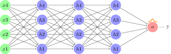
Figure 2: DKL for the outcome regression models.

Another component of our proposed model is the outcome regression models. Fit a DKL model for outcome regression models (Fig. 2) at each time $m$, recursively from the last time point to the first time point. The outcome regression models are fitted and evaluated for all subjects that are uncensored at each time point. At each iteration, DKL is trained for a outcome regression model firstly. Then DKL predicted an intermediate outcome used in the next iteration. The input is transformed with a deep neural network according to Eq. (8). At the iteration $m$, an outcome regression model is fitted with the weight $W_{m}$ as a covariate. The input is the past treatments $\bar{T}_{m}$, the past observed confounders $\bar{L}_{m+1}$, the past outcomes $\bar{Y}_{m}$ and the weight $W_{m}$. And an intermediate outcome is predicted by the estimated outcome regression model with the weight $W_{m}^{md}$ as a covariate. The intermediate outcome is used to train the DKL in the next iteration. The input to get the intermediate outcome is the treatments $\bar{T}_{m-1},d_{m}$, the past observed confounders $\bar{L}_{m+1}$, the past outcomes $\bar{Y}_{m}$ and the modified weight $W_{m}^{md}$. The output is a multivariate Gaussian distribution (Eq. (6)), which include a mean value (Eq. (3)) and a variance value (Eq. (4)). The intermediate outcome is the mean value of the Gaussian distribution.

input : Treatments $T$, confounders $L$ and outcomes $Y$

output : Causal effects

1 for $m\leftarrow 0$ to $K$ do

2      

3      Fit models for the treatment models relating to both the treatment and censoring mechanism (Eq. (10) and (11)).

4       Compute $\hat{W}_{m}$ according to Eq. (16) and $\hat{W}^{md}_{m}$ according to Eq. (17).

5      

6      Set $\hat{Q}_{K+1}=Y$. Then, for $m=K,K-1,\dots,0$,

7         a) Fit a model $h(\bar{T}_{m},\bar{L}_{m+1},\bar{Y}_{m};\theta)$ with a covariate $\hat{W}_{m}$ for the conditional expectation $\mathbb{E}[\hat{Q}_{m+1}|\bar{T}_{m},\bar{L}_{m+1},C_{m+1}=0,\bar{Y}_{m}]$ with subjects that $C_{m+1}=0$.

8         b) Predict the outcome $\hat{Q}_{m}$ based on the model $\hat{h}(\bar{T}_{m-1},d_{m},\bar{L}_{m+1},\bar{Y}_{m};\hat{\theta})$ using the covariate $\hat{W}^{md}_{m}$ rather than $\hat{W}_{m}$ with subjects that $C_{m}=0$.

9       The dynamic causal effect is calculated by the mean of the predicted outcome, that is $\mathbb{E}[\hat{Q}_{0}]$.

10 end for

Algorithm 1 TS Algorithm

The whole procedure of our algorithm is summarised in Algorithm 1.

We use a logistic regression model on the assumption of a linear additive form of covariates to estimate time-varying inverse probability weights. Then, we apply DKL [30] for the outcome regression models. We name our two-step (TS) model with DKL for the outcome regression models, TS-DKL.

V Experiments

We design a series of experiments to evaluate the effectiveness of the proposed model. First, we introduce data simulations for dynamic treatment regimes. Then, we present the experimental setting and baseline methods, followed by an analysis of the experimental results. The experiments include the property analyses of the proposed model and the evaluation of the performance of the proposed model on simulated data.

$$T_{-1} \sim B(p=1)$$ (18)

$$V^{1} \sim B(p=4392/5826)$$

$$V^{2}|\overline{\mathcal{D}} \sim\left\{\begin{array}[]{ll}{B(p=2222/4392)}&{\text{ if }\quad V^{1}=1}\\ {B(p=758/1434)}&{\text{ if }\quad V^{1}=0}\end{array}\right.$$

$$V^{3}|\overline{\mathcal{D}} \sim U(1,5)$$

$$L_{0}^{1}|\overline{\mathcal{D}} \sim\left\{\begin{array}[]{ll}{N_{[0,10000]}(650,350)}&{\text{ if }V^{1}=1}\\ N_{[0,10000]}(720,400)&{\text{ if }V^{1}=0}\end{array}\right.$$

$$\tilde{L}_{0}^{1}|\overline{\mathcal{D}} \sim N\left(\left(L_{0}^{1}-671.7468\right)/(10\cdot 352.2788)+1,0\right)$$

$$L_{0}^{2}|\overline{\mathcal{D}} \sim N_{[0.06,0.8]}\left(0.16+0.05\cdot\left(L_{0}^{1}-650\right)/650,0.07\right)$$

$$\tilde{L}_{0}^{2}|\overline{\mathcal{D}} \sim N\left(\left(L_{0}^{2}-0.1648594\right)/(10\cdot 0.06980332)+1,0\right)$$

$$L_{0}^{3}|\overline{\mathcal{D}} \sim\left\{\begin{array}[]{ll}N_{[-5,5]}(-1.65+0.1\cdot V^{3}+0.05\cdot(L_{0}^{1}-650)/650+0.05\cdot(L_{0}^{2}-16)/16,1)&\text{ if }V^{1}=1\\ N_{[-5,5]}(-2.05+0.1\cdot V^{3}+0.05\cdot(L_{0}^{1}-650)/650+0.05\cdot(L_{0}^{2}-16)/16,1)&\text{ if }V^{1}=0\end{array}\right.$$

$$C_{0}|\overline{\mathcal{D}} \sim B(p=0)$$

$$Y_{0}|\overline{\mathcal{D}} \sim N_{[-5,5]}(-2.6+0.1\cdot I(V^{3}>2)+0.3\cdot I(V^{1}=0)+(L_{0}^{3}+1.45),1.1)$$

$$T_{0}|\overline{\mathcal{D}} \sim\left\{\begin{array}[]{ll}B(p=1)&\text{ if }T_{-1}=1\\ B\left(p=1/\left(1+\exp\left(-\left[-2.4+0.015\cdot\left(750-L_{0}^{1}\right)+5\cdot\left(0.2-L_{0}^{2}\right)-0.8\cdot L_{0}^{3}\right]\right)\right)\right)&\text{ if }T_{-1}=0\end{array}\right.$$

For $$k>0:$$

$$L_{k}^{1}|\overline{\mathcal{D}} \sim\left\{\begin{array}[]{ll}N_{[0,10000]}\left(13\cdot\log(k\cdot(1034-662)/8)+L_{k-1}^{1}+2\cdot L_{k-1}^{2}+2\cdot L_{k-1}^{3}+2.5\cdot T_{k-1},50\right)&\text{ if }k\in\{1,2,3,4\}\\ N_{[0,10000]}\left(4\cdot\log(k\cdot(1034-662)/8)+L_{k-1}^{1}+2\cdot L_{k-1}^{2}+2\cdot L_{k-1}^{3}+2.5\cdot T_{k-1},50\right)&{\text{ if }k\in\{5,6,7,8\}}\\ N_{[0,10000]}\left(L_{k-1}^{1}+2\cdot L_{k-1}^{2}+2\cdot L_{k-1}^{3}+2\cdot L_{k-1}^{3}+2.5\cdot T_{k-1},50\right)&\text{ if }k\in\{9,10,11,12\}\end{array}\right.$$

$$L_{k}^{2}|\overline{\mathcal{D}} \sim N_{[0.06,0.8]}\left(L_{k-1}^{2}+0.0003\cdot\left(L_{k}^{1}-L_{k-1}^{1}\right)+0.0005\cdot\left(L_{k-1}^{3}\right)+0.0005\cdot T_{k-1}\cdot\tilde{L}_{0}^{1},0.02\right)$$

$$L_{k}^{3}|\overline{\mathcal{D}} \sim N_{[-5,5]}\left(L_{k-1}^{3}+0.0017\cdot\left(L_{k}^{1}-L_{k-1}^{1}\right)+0.2\cdot\left(L_{k}^{2}-L_{k-1}^{2}\right)+0.005\cdot T_{k-1}^{2}\cdot{\tilde{L}_{0}}^{2},0.5\right)$$

$$C_{k}|\overline{\mathcal{D}} \sim B\left(max(p=1/\left(1+\exp\left(-\left[-6+0.01\cdot\left(750-L_{k}^{1}\right)+1\cdot\left(0.2-L_{k}^{2}\right)-0.65\cdot L_{k}^{3}-T_{k-1}\right]\right)\right),0.05)\right)$$

$$Y_{k}|\overline{\mathcal{D}} \sim N_{[-5,5]}\left(Y_{k-1}+0.00005\cdot\left(L_{k}^{1}-L_{k-1}^{1}\right)-0.000001\cdot\left(\left(L_{k}^{1}-L_{k-1}^{1}\right)\cdot\sqrt{\tilde{L}_{0}^{1}}\right)^{2}+0.01\cdot\left(L_{k}^{2}-L_{k-1}^{2}\right)-\right.$$

$$0.0001\cdot\left(\left(L_{k}^{2}-L_{k-1}^{2}\right)\cdot\sqrt{\tilde{L}_{0}^{2}}\right)^{2}+0.07\cdot\left(\left(L_{k}^{3}-L_{k-1}^{3}\right)\cdot\left(L_{0}^{3}+1.5135\right)\right)-0.001\cdot\left(\left(L_{k}^{3}-L_{k-1}^{3}\right)\cdot\left(L_{0}^{3}+1.5135\right)\right)^{2}$$

$$+\left.0.005\cdot T_{k-1}+0.075\cdot T_{k-2}+0.05\cdot T_{k-1}\cdot T_{k-2},2.5\right)$$

$$T_{k}|\overline{\mathcal{D}} \sim\left\{\begin{array}[]{ll}B(p=1)&\text{ if }T_{k-1}=1\\ B\left(p=1/\left(1+\exp\left(-\left[-2.4+0.015\cdot\left(750-L_{k}^{1}\right)+5\cdot\left(0.2-L_{k}^{2}\right)-0.8\cdot L_{k}^{3}+0.8\cdot k\right]\right)\right)\right)&\text{ if }T_{k-1}=0\end{array}\right.$$

V-A Data simulation

Since rare ground truth is known in real non-experimental observational data, we use simulation data from LTMLE [4] with a slight revision to fit the problem setting. We run ten simulations for the data generation process. We simulate a binary treatment indicator, a censoring indicator, three static covariates, three time-dependent covariates and an outcome variable with twelve time points using causal structural equations Eq. (18) by R-package simcausal [33].

We simulate the static covariates ($V^{1},V^{2},V^{3}$), which refers to region, sex, age, respectively. The time-dependent covariates ($L^{1}_{k},L^{2}_{k},L^{3}_{k}$) refer to CD4 count, CD4%, and WAZ at time $k$, respectively. We simulate a binary treatment indicator $T_{k}$, referring to whether ART was taken at time $k$ or not; a censoring indicator $C_{k}$, describing whether the patient was censored (failing to follow the study) at time $k$; and a continuous outcome $Y_{k}$, which refers to HAZ at time $k$. The binary variable is simulated by a Bernoulli ($B$) distribution. We use uniform ($U$) distribution, normal ($N$) distribution, and truncated normal distribution which is denoted by $N_{[a,b]}$ where $a$ and $b$ are the truncation levels, to simulate continuous variables. When values are simulated in truncated normal distributions, if the values are smaller than $a$, they are replaced by a random draw from a $U(a_{1},a_{2})$ distribution. Conversely, if the values are greater than $b$, then the replacing values are drawn from a $U(b_{1},b_{2})$ distribution. The values of ($a_{1},a_{2},b_{1},b_{2}$) are (0, 50, 5000, 10000) for $L_{1}$, (0.03,0.09,0.7,0.8) for $L_{2}$, and $(-10,3,3,10)$ for both $L_{3}$ and $Y$. The notation $\bar{\mathcal{D}}$ denotes the data that have been observed before the time point. All the subjects are untreated before the study and are represented by $T_{-1}=0$, and all the subjects are uncensored at the baseline $k=0$.

The goal is to estimate the mean HAZ at time $K+1$ for the subjects. We consider four treatment regimes (Eq. (19)), where two treatment regimes are static, and the other two are dynamic.

$$\bar{d}_{k}^{1}=\left\{c_{k}=0\text{ and }t_{k}=1\text{ for all }k\right.$$ (19)

$$\bar{d}_{k}^{2}=\left\{\begin{array}[]{ll}c_{k}=0\text{ and }t_{k}=1&\text{ if condition 1}\\ c_{k}=0\text{ and }t_{k}=0&\text{ otherwise }\end{array}\right.$$

$$\bar{d}_{k}^{3}=\left\{\begin{array}[]{ll}c_{k}=0\text{ and }t_{k}=1&\text{ if condition 2}\\ c_{k}=0\text{ and }t_{k}=0&\text{ otherwise }\end{array}\right.$$

$$\bar{d}_{k}^{4}=\left\{c_{k}=0\text{ and }t_{k}=0\text{ for all }k\right.$$

$$\text{condition 1:}\text{ CD4 count }_{k}^{\bar{d}_{k}^{2}}<750\text{ or }\mathrm{CD}4\%_{k}^{\bar{d}_{k}^{2}}<25\%$$

$$\text{ or }\mathrm{WAZ}_{k}^{\bar{d}_{k}^{2}}<-2\text{ or }t_{k-1}=1$$

$$\text{condition 2:}\text{ CD4 count }_{k}^{\bar{d}_{k}^{3}}<350\text{ or }\mathrm{CD}4\%_{k}^{\bar{d}_{k}^{3}}<15\%$$

$$\text{ or }\mathrm{WAZ}_{k}^{\bar{d}_{k}^{3}}<-2\text{ or }t_{k-1}=1.$$

The first and fourth treatment regimes are static. The first treatment regime “always treat” means all uncensored subjects are treated at each time point during the study. The last treatment regime “never treat” means all uncensored subjects are not treated at each time point during the study. The second and third treatment regimes, “750s” and “350s”, mean uncensored subjects receive treatments until their CD4 reaches a particular threshold. Our proposed method is designed for the dynamic treatment regimes “750s” and “350s”.

V-B Experimental setting

The experimental setting is described briefly in this section. The target is to evaluate the average dynamic causal effect, under a treatment regime of interest, from the observational data. The evaluation metric for estimation is the mean absolute error (MAE) between the estimated average causal effect and the ground truth.

We use the Python package gpytorch [34] to implement the DKL model [35, 30]. We use a fully connected network that has the architecture of three hidden layers with 1000, 500, and 50 units. The activation function is ReLU. The optimization method is implemented in Adam [36] with a learning rate of 0.01. We train the deep kernel learning model for five iterations, and the DKL model uses a GridInterpolationKernel (SKI) with an RBF base kernel. A neural network feature extractor is used to pre-process data, and the output features are scaled between 0 and 1.

V-C Baseline Methods

We present the baseline methods which are the inverse probability of treatment weighting (IPTW) [2], marginal structural model (MSM) [19, 28], sequential g-formula (Seq) [3], and longitudinal targeted maximum likelihood estimation (LTMLE) [4, 5]. The comparative methods and publication references are listed in Table III. IPTW and MSM only apply treatment models, sequential g-formula only applies outcome regression models, and LTMLE and our proposed method apply both the treatment models and outcome regression models. We describe the general implementation procedure for these comparative methods as follows.

Given a fixed regime $\bar{d}$, $\bar{g}_{k}(\bar{L}_{k+1},\bar{Y}_{k})$ is defined as Eq. (20),

$$\bar{g}_{k}(\bar{L}_{k+1}, \bar{Y}_{k})=\prod_{m=0}^{k}\Pr(T_{m}=d_{m}|\bar{T}_{m-1}=\bar{d}_{m-1},C_{m}=0,\bar{L}_{m},\bar{Y}_{m})$$ (20)

$$\times\prod_{m=1}^{k+1}\Pr(C_{m}=0|\bar{T}_{m-1}=\bar{d}_{m-1},C_{m-1}=0,\bar{L}_{m},\bar{Y}_{m-1}),$$

where $\bar{g}_{0}(\bar{L}_{1},Y_{0})=\Pr(T_{0}=d_{0}|L_{0},Y_{0})\times\Pr(C_{1}=0|T_{0}=d_{0},\bar{L}_{1},Y_{0}).$ $\bar{g}_{n,k}(\bar{L}_{k+1},\bar{Y}_{k})$ denotes the estimated values of $\bar{g}_{k}(\bar{L}_{k+1},\bar{Y}_{k})$.

Now we describe the general procedure of LTMLE [4, 5]. Before the outcome regression models with respect to the target variable are fitted to the observational data, we calculate the probabilities $\bar{g}_{n,k}(\bar{L}_{k+1},\bar{Y}_{k})$ for each subject that follows the given treatment regime $\bar{d}$. The following steps can be implemented as follows: Set $\bar{Q}_{n,K+1}=Y$ (the continuous outcome should be rescaled to [0,1] using the true bounds and be truncated to (a,1-a), such as a = 0.0005). Then for $k=K,...,1$,

1. Fit a model for $\mathbb{E}[\bar{Q}_{n,k+1}|C_{k+1}=0,\bar{T}_{k},\bar{L}_{k+1}]$. The model is fitted on all subjects that are uncensored until time $k+1$.

2. Plug in $\bar{T}_{k}=\bar{d}_{k}$ based on the treatment regime $\bar{d}_{k}$, predict the conditional outcome $\bar{Q}_{n,k}$ with the regression model from step 1 for all subjects with $C_{k}=0$.

3. • Plug in $\bar{T}_{k}=\bar{d}_{k}$ based on the treatment regime $\bar{d}_{k}$, get $\bar{Q}_{k}$ with the regression model from step 1 for all subjects with $C_{k+1}=0$.

   • Construct the “clever covariate”

     $$\footnotesize CL_{k}(C_{k+1},\bar{T}_{k}=\bar{d}_{k},\bar{L}_{k+1},\bar{Y}_{k})=\frac{I(C_{k+1}=0,\bar{T}_{k}=\bar{d}_{k})}{\bar{g}_{n,k}(\bar{L}_{k+1},\bar{Y}_{k})},$$ (21)

     where $I(\cdot)$ is an indicator function for a logical statement.

   • Run a no-intercept logistic regression. The outcome refers to $\bar{Q}_{n,k+1}$, the offset is $\text{logit}(\bar{Q}_{k})$, and the covariate $CL_{k}$ is the unique covariate. The model fits all subjects that are uncensored until time $k+1$ and followed the treatment regime $\bar{T}_{k}=\bar{d}_{k}$. Let $\hat{\epsilon}$ be the estimated coefficient of $H_{k}$.

   • Obtain the new predicted value of $\bar{Q}_{n,k}$ for all subjects with $C_{k}=0$ by

     $$\bar{Q}_{n,k}=\text{expit}(\text{logit}(\bar{Q}_{n,k})+\frac{\hat{\epsilon}_{k}}{\bar{g}_{n,k}(\bar{L}_{k+1},\bar{Y}_{k})}).$$ (22)

4. An estimate of the dynamic causal effect is obtained by taking the mean of $\bar{Q}_{n,1}$ over all subjects; the mean is transformed back to the original scale for the continuous outcome.

The sequential g-formula (the sequential g-computation estimator or the iterated conditional expectation estimator) can be estimated by step 1, step 2, and step 4 of LTMLE.

IPTW uses the time-varying inverse probability weights to create pseudo-populations in order to estimate the dynamic causal effect. The IPTW estimator for dynamic causal effect at time $k$ can be obtained from $\mathbb{E}[Y\cdot I(C_{k+1}=0,\bar{T}_{k}=\bar{d}_{k})/\bar{g}_{n,k}(\bar{L}_{k+1},\bar{Y}_{k})]$, where $I(\cdot)$ is the indicator function.

To estimate the dynamic causal effect, we fit the ordinary linear regression model $\mathbb{E}[Y^{\bar{d}_{k},\bar{c}_{k+1}=0}]=\theta_{0}+\theta_{1}cum(\bar{d}_{k})$ to estimate the parameters of the marginal structural model (MSM). The $cum(\bar{d}_{k})$ represents the cumulative treatment in $k$ time points. MSM is fitted in the pseudo-population created by inverse probability weights. That is, we use weighted least squares with inverse probability weights.

To improve the performance of the outcome regression models, Super Learner [37, 38] is often used. Super Learner is an ensemble machine learning method. We test three different sets of learners for outcome regression models which are applied in sequential g-formula, LTMLE, and our model. Learner 1 consists of ordinary linear regression models, learner 2 contains ordinary linear regression models and random regression forests, and learner 3 adds a multi-layer perceptron (MLP) algorithm with a hidden layer with 128 units in addition to the algorithms used in learner 2. We represent sequential g-formula with learners 1, 2 and 3 as Seq-L1, Seq-L2 and Seq-L3, respectively. We represent similarly in LTMLE and our proposed method with the three learners as the outcome regression models. In order to show the effectiveness of DKL, we also implement our proposed method with a fully connected neural network (TS-NN) as the outcome regression model. The network has the architecture of three hidden layers with 128, 64, and 32 units. The activation function is the ReLU activation function and dropout regularization is used. We train our outcome regression model for 5 epochs with a dropout rate of 0.9. The optimization method is implemented in Adam [36] with a learning rate of 0.01.

V-D Propensity score truncation for positivity problems

To calculate the dynamic causal effect, all baseline methods excluding sequential g-formula have treatment models relating to both the treatment and censoring mechanism. The treatment models for the $K+1$ time points is $2K+2$, that is, $K+1$ treatment models relating to the treatment assignment mechanism, and $K+1$ treatment models relating to the censoring mechanism. In long-term follow-up causal studies, the treatment models need to regress on high-dimensional features using small-size samples at each time point. The estimated treatment and uncensored probabilities may be small and the cumulative probabilities would be close to zero. This may lead to near-positivity violations.

We deal with small treatment and uncensored probabilities by truncating them at a bound. We truncate both the estimated treatment and uncensored probabilities at a lower bound 0.1 and a higher bound 0.9. The truncation improves the stability of the performance for the methods. In addition, we normalize the weights by their sum, that is a new weight $W_{i}=W_{i}/\sum_{j}W_{j}$. For all methods that apply the treatment models, we use standard logistic regression models for the treatment models relating to both the treatment and censoring mechanism.

V-E Evaluation of a long follow-up time and declining sample size

Fewer subjects follow the study as the causal study progresses. If a subject is uncensored at time $k$, then the subject has followed all the studies in previous time points. If a subject is censored at time $k$, then the variables related to the subject are unobserved from time $k+1$. The estimation of dynamic causal effects is necessarily restricted to uncensored subjects. Another challenge is that time-dependent confounders are affected by prior treatments and influence future treatments and outcomes, hence it is necessary for the time-dependent confounders to be adjusted. In long-term follow-up causal studies, high-dimensional adjustment confounders exist. All baseline methods are required to fit the data of uncensored subjects at each time point. As a result, the estimators need to handle a reduced sample size and high-dimensional confounders at each time point.

TABLE IV: The number of features to regress increases, but the sample size of the uncensored subjects to regress declines, over time. As the time-dependent confounding exists, more features need to regress but less subjects are available in a longer study. The label “uncensored” refers to the uncensored subjects. The labels “750s” and “350s” refer to the uncensored subjects who have followed the dynamic treatment regime.

Time Point	1	2	3	4	5	6	7	8	9	10	11	12
Dimension	11	16	21	26	31	36	41	46	51	56	61	66
Uncensored	883	821	777	736	699	664	632	598	571	541	514	485
750s	480	429	397	374	353	333	315	297	283	266	250	235
350s	564	434	386	355	330	308	287	266	250	232	215	199

We show that fewer subjects are available with more features to regress over time in Table IV. There are 485 uncensored subjects and 66 adjustment confounders at the twelfth time point, that is $K=11$. The number of uncensored subjects at the time point of interest is quite small. It is seen that the size of uncensored subjects is declining as the study progresses (the time point increases) and it is noted that the number of features to regress at each time point increases. Regression estimators need to fit data with increasing features but smaller available observations. Table IV show that the number of uncensored subjects following the dynamic treatment regime of interest (“750s” and “350s”) is even smaller than the number of uncensored subjects.

The limited number of uncensored subjects who follow the treatment regime of interest makes it challenging to estimate the dynamic causal effect. Some estimators (such as LTMLE and IPTW) need to use the information from the limited number of uncensored subjects who followed the treatment regime of interest. However, these estimators may have an unstable estimation in a long follow-up study. We investigate the trend of two dynamic treatment regimes, “750s” and “350s”, to show the declining, limited sample size of subjects who followed the treatment regimes in Fig. 3. The size of the uncensored subjects reduces as the study progresses. This is also true for the uncensored subjects following the treatment regime of interest, where Fig. 3 shows that the sample size of the uncensored subjects is much larger than those uncensored subjects who followed a special treatment regime. It is usually easier for a model to achieve stable performance by fitting the data with more observations than fitting the data with less observations. The treatment models of our proposed model fit the data of uncensored subjects. The treatment models of LTMLE fit the data of uncensored subjects who followed the dynamic treatment regime. This makes it possible for our proposed model to achieve a more stable estimation.

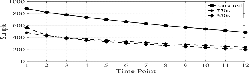
Figure 3: The sample size of subjects declines as the study progresses. The label “censored” represents the number of subjects who are uncensored. The label “750s” represents the number of uncensored subjects who receive the dynamic treatment regime “750s”. The label “350s” represents the uncensored subjects who follow the treatment regime “350s”.

V-F Experimental analysis of our proposed method

We analyse the influence of the number of subjects applied in the treatment models. The treatment models of LTMLE and IPTW need to fit the limited number of uncensored subjects who followed the treatment regime of interest at each time point $k$. Unlike LTMLE and IPTW, the treatment models of our model fit on all subjects who are uncensored at each time $k$. As more subjects are available in the treatment models, the estimate of our proposed method for a dynamic causal effect may be more stable. DKL is applied in the outcome regression model at each time point. DKL is suitable for the data which has high features but a small number of observations. We show the MAE estimates for the two dynamic treatment regimes, “750s” and “350s”, in Fig. 4 and Fig. 5. The MAE for the treatment regime, “750s”, varies between 0 and 2 for different time points. The MAE for the treatment regime, “350s”, varies between 0 and about 2 for different time points. It is interesting that bias reduces as the time point increases. Next, we focus on the experimental analysis of the long follow-up, that is the time point 11 and 12. As illustrated in Fig. 4 and Fig. 5, the estimates of the dynamic causal effect with the given dynamic treatment regimes (“750s” and “350s”) at different time points (the time point 11 and 12 ) do not vary significantly. The figures show our model provides stable estimates for the long-term follow-up causal study. It is also noted that the bias of the dynamic causal effect at the time points 11 and 12 is small. These results indicate that our proposed method is able to achieve a stable and effective estimate in a long-term follow-up study.

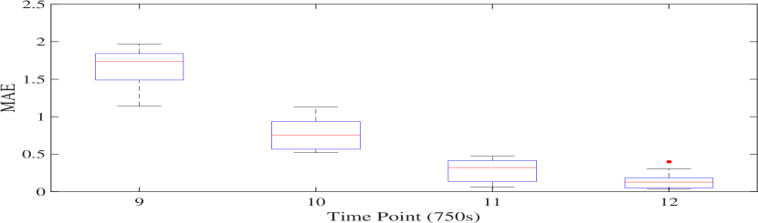
Figure 4: The experimental analysis for the performance (MAE) given the dynamic treatment regime, “750s”, at different time $K+1=9,10,11,12$.

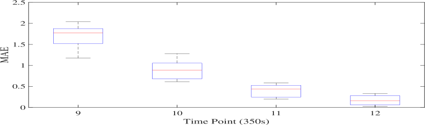
Figure 5: The experimental performance (MAE) of average causal effects for the treatment rule “350s” at different time points. We show the MAE for time points 9, 10, 11 and 12 ($K=8,9,10,11$).

Next, we analyse DKL’s ability to capture the variance for the causal prediction of a subject. For every predicted value, DKL also produces its variance. Ten observations were selected to show the predicted values $\hat{y}^{\bar{d}_{K},\bar{c}_{K+1}=0}$ and the variances of these predicted values. Fig. 6 show the predicted values and its five standard deviation. The variances are presented by the shade area in the figure. It can be seen that the variance is small for each observation. DKL describes the uncertainty of predictions through these small variances.

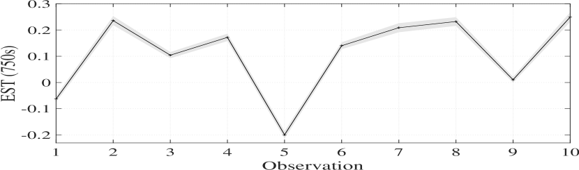
Figure 6: The plot shows the estimated value $\hat{y}^{\bar{d}_{K},\bar{c}_{K+1}=0}$ and its variance for each observation. The number of the observations is 10. The time point is $K$+1 = 12.

V-G Evaluation of dynamic causal effect with synthetic data

The results of the experiment using synthetic data are analysed in this section. We aim to estimate the dynamic causal effect $\mathbb{E}[Y^{\bar{d}_{K},\bar{c}_{K+1}=0}]$. The real dynamic causal effects are directly obtainable within the simulated data. The performance is evaluated using the MAE between the estimated causal effect and the real causal effect, for all ten simulations. Our proposed method (TS-DKL) is designed for the dynamic treatment regimes, “750s” and “350s”. The comparative methods and publication references are listed in Table III. The outcome regression models of sequential g-formula, LTMLE and our proposed method are equipped with three different sets of learners, detailed in Section V-C. A neural network is only implemented in the outcome regression model of our proposed method (TS-NN). TS-NN is used to evaluate the effectiveness of the DKL.

We summarise the experimental results of the estimates for the dynamic treatment regimes, “750s” and “350s”, in time points 11 and 12 in Table V. Table V shows that no models can obtain the best results for all estimates for the two dynamic treatment regimes at the two different time points. We can observe that TS-DKL obtains the best results (three treatments out of the four), followed by IPTW (one treatment out of the four), in the two time points. TS-DKL achieves the second best experimental performance for the dynamic treatment regime “750s” at the time point 12, where the experimental performance of IPTW is the best. Compared with TS-NN, TS-DKL achieves better experimental performance in all dynamic treatment regimes, hence we conclude that applying DKL in the outcome regression models is effective. The reason for this is the outcome regression model needs to fit the data, which has high dimensions but is small in terms of sample size. A deep neural network usually works poorly with a limited number of observations. This is the main reason that DKL is applied in the outcome regression models. Compared with the three TS-L* models, TS-L1, TS-L2, and TS-L3, we believe DKL has a strong ability to capture the complex treatment, time-varying confounders, and outcome relationships. The reason for this is that the only difference between TS-DKL and the three TS-L* models is that the different methods are applied in the outcome regression models. As the performance of TS-DKL is the best one in both two time points, TS-DKL has a strong ability to capture the causal effects of dynamic treatment regimes in a long-term follow-up causal study.

TABLE V: The experimental results showing MAE from estimates of dynamic causal effect for time points 11 and 12 ($K=10,11$). TS-DKL is our model with outcome regression models using deep kernel learning.

Time points	11		12
Treatment	750s	350s	750s	350s
IPTW	0.2025	0.3042	0.0835	0.1932
MSM	2.9740	3.0742	2.8150	3.0314
Seq-L1	0.3043	0.1983	0.2997	0.1959
Seq-L2	0.2363	0.1806	0.2742	0.1861
Seq-L3	0.2536	0.2261	0.2739	0.2171
LTMLE-L1	0.1744	0.1936	0.1863	0.1927
LTMLE-L2	0.1475	0.1744	0.1658	0.1805
LTMLE-L3	0.1324	0.1801	0.1724	0.1935
TS-L1	0.3031	0.1940	0.2926	0.1996
TS-L2	0.1905	0.1900	0.2215	0.1887
TS-L3	0.2197	0.2022	0.2650	0.2094
TS-NN	0.3203	0.3751	0.3286	0.2726
TS-DKL	0.1253	0.1450	0.1528	0.1650

We analyse the experiment results for our proposed method for the static treatment regimes. TS-DKL is designed to estimate the dynamic causal effects for the dynamic treatment regimes. It is still unknown whether our proposed method is able to achieve a comparative experimental performance for static treatment regimes or not. Table VI show the experimental performance of the baseline methods for the static treatment regimes, “always treat” and “never treat”. TS-DKL obtains the best experimental performance under the static treatment regime “always treat”, and Seq-L3 obtains the best experimental performance under the static treatment regime “never treat”, for time point 11. IPTW obtains the best experimental performance under the static treatment regime “always treat”, and TS-L2 obtains the best experimental performance under the static treatment regime “never treat”, for time point 12. It is noted that the experimental performance of LTMLE-L3 and TS-DKL is relatively better than the other baseline methods, excluding IPTW, under the static treatment regime “always treat”, for time point 12. Thus, the experimental performance of TS-DKL under the treatment regime “always treat” is relatively better than the other methods. All the baseline methods obtain poor estimates under the treatment regime “never treat”. One potential reason for this is the limited number of uncensored subjects who followed the treatment regime “never treat”, which reduces the models’ ability to capture the data generating process. Moreover, the limited number of subjects particularly affect the models IPTW, MSM and LTMLE.

TABLE VI: Experimental analysis with MAE of the estimated causal effects (time points 11 and 12) for the static treatment regimes. The TS-DKL is our model with a deep kernel learning as the outcome regression model.

Time points	11		12
Treatment	all	never	all	never
IPTW	0.1798	0.7186	0.0583	0.6255
MSM	3.1081	4.3238	3.2230	5.4558
Seq-L1	0.3323	0.3216	0.3270	0.3255
Seq-L2	0.2468	0.3059	0.2935	0.3172
Seq-L3	0.2848	0.2692	0.3109	0.2979
LTMLE-L1	0.1795	0.5780	0.1908	0.5502
LTMLE-L2	0.1444	0.5463	0.1696	0.5119
LTMLE-L3	0.1445	0.5390	0.1509	0.5279
TS-L1	0.3301	0.3361	0.3175	0.3497
TS-L2	0.2042	0.3489	0.2376	0.2538
TS-L3	0.2724	0.3268	0.2368	0.2664
TS-NN	0.3109	0.7006	0.3433	0.4067
TS-DKL	0.1251	0.5150	0.1595	0.4792

We analyse the bias introduced by the outcome regression models. The outcome regression models are applied in sequential g-formula, LTMLE and our proposed method. The results of the empirical standard deviations (ESD) of the estimates for dynamic causal effect in time points 11 and 12 are shown in Table VII. TS-DKL performs stably under both dynamic treatment regimes in the two different time points. Seq-L2 obtains stable experimental performance under the dynamic treatment regime “350s”, and obtains relatively larger ESD under the dynamic treatment regime “750s”. TS-L1 and TS-L2 have stable performance under the dynamic treatment regime, “350s”, in time point 12. We can conclude that DKL is an effective method to implement in the outcome regression models. By comparising of TS-NN and TS-DKL, it can be seen that Bayesian deep learning introduces robustness in the small-sized data. The neural network applied in TS-NN performs unstably for the small-sized observations.

TABLE VII: The experimental results show the ESD from the estimates of dynamic causal effect for time points 11 and 12 ($K=10,11$). TS-DKL is our model with DKL as the outcome regression model.

Time points	11		12
Treatment	750s	350s	750s	350s
Seq-L1	0.2896	0.1649	0.3086	0.2112
Seq-L2	0.2332	0.1420	0.2873	0.2043
Seq-L3	0.2529	0.1756	0.2908	0.2323
LTMLE-L1	0.1942	0.1878	0.2408	0.2128
LTMLE-L2	0.1942	0.1878	0.2408	0.2128
LTMLE-L3	0.1619	0.1610	0.2256	0.2136
TS-L1	0.2812	0.1588	0.3000	0.2084
TS-L2	0.1955	0.1721	0.2456	0.2056
TS-L3	0.2534	0.2278	0.2931	0.2343
TS-NN	0.4914	0.4915	0.3370	0.3374
TS-DKL	0.1464	0.1415	0.1829	0.2072

VI Conclusion and Future Work

We proposed a deep Bayesian estimation for dynamic treatment regimes with long-term follow-up. Our two-step method combines the outcome regression models with treatment models and improves the target quantity using the information of inverse probability weights on uncensored subjects. Deep kernel learning is applied in the outcome regression models to capture the complex relationships between confounders, treatments, and outcomes. The experiments have verified that our method generally achieves both good performance and stability.

Currently, our approach lacks an analysis of asymptotic properties. The work on the analytic estimation of standard errors and confidence intervals is yet to be undertaken. In future work, we will provide theoretical guarantees for standard errors and confidence intervals.

References

- [1] P. Spirtes and K. Zhang, “Causal discovery and inference: concepts and recent methodological advances,” in Applied informatics, vol. 3, no. 1. SpringerOpen, 2016, p. 3.
- [2] P. C. Austin, “An introduction to propensity score methods for reducing the effects of confounding in observational studies,” Multivariate behavioral research, vol. 46, no. 3, pp. 399–424, 2011.
- [3] L. Tran, C. Yiannoutsos, K. Wools-Kaloustian, A. Siika, M. Van Der Laan, and M. Petersen, “Double robust efficient estimators of longitudinal treatment effects: comparative performance in simulations and a case study,” The international journal of biostatistics, vol. 15, no. 2, 2019.
- [4] M. Schomaker, M. A. Luque-Fernandez, V. Leroy, and M.-A. Davies, “Using longitudinal targeted maximum likelihood estimation in complex settings with dynamic interventions,” Statistics in medicine, vol. 38, no. 24, pp. 4888–4911, 2019.
- [5] M. J. van der Laan and S. Rose, Targeted Learning in Data Science: Causal Inference for Complex Longitudinal Studies. Springer, 2018.
- [6] H. Huang, C. Xu, and S. Yoo, “Bi-directional causal graph learning through weight-sharing and low-rank neural network,” in 2019 IEEE International Conference on Data Mining (ICDM). IEEE, 2019, pp. 319–328.
- [7] R. Cui, P. Groot, and T. Heskes, “Robust estimation of gaussian copula causal structure from mixed data with missing values,” in 2017 IEEE International Conference on Data Mining, ICDM 2017, New Orleans, LA, USA, November 18-21, 2017, 2017, pp. 835–840.
- [8] F. Xie, R. Cai, Y. Zeng, J. Gao, and Z. Hao, “An efficient entropy-based causal discovery method for linear structural equation models with IID noise variables,” IEEE Trans. Neural Networks Learn. Syst., vol. 31, no. 5, pp. 1667–1680, 2020.
- [9] K. Yu, L. Liu, J. Li, and H. Chen, “Mining markov blankets without causal sufficiency,” IEEE Trans. Neural Networks Learn. Syst., vol. 29, no. 12, pp. 6333–6347, 2018.
- [10] F. Liu and L. Chan, “Causal inference on multidimensional data using free probability theory,” IEEE Trans. Neural Networks Learn. Syst., vol. 29, no. 7, pp. 3188–3198, 2018.
- [11] R. Cai, Z. Zhang, Z. Hao, and M. Winslett, “Sophisticated merging over random partitions: A scalable and robust causal discovery approach,” IEEE Trans. Neural Networks Learn. Syst., vol. 29, no. 8, pp. 3623–3635, 2018.
- [12] L. Yao, S. Li, Y. Li, M. Huai, J. Gao, and A. Zhang, “Representation learning for treatment effect estimation from observational data,” in Proceedings of the 32nd International Conference on Neural Information Processing Systems. Curran Associates Inc., 2018, pp. 2638–2648.
- [13] L. Yao, S. Li, Y. Li, and M. Huai, “Ace: Adaptively similarity-preserved representation learning for individual treatment effect estimation,” in 2019 IEEE International Conference on Data Mining (ICDM). IEEE, 2019, pp. 1432–1437.
- [14] F. Tan, Z. Wei, A. Pani, and Z. Yan, “User response driven content understanding with causal inference,” in 2019 IEEE International Conference on Data Mining (ICDM). IEEE, 2019, pp. 1324–1329.
- [15] N. Kreif and K. DiazOrdaz, “Machine learning in policy evaluation: New tools for causal inference,” in Oxford Research Encyclopedia of Economics and Finance, 2019.
- [16] P. R. Hahn, J. S. Murray, C. M. Carvalho et al., “Bayesian regression tree models for causal inference: regularization, confounding, and heterogeneous effects,” Bayesian Analysis, 2020.
- [17] A. Lin, J. Lu, J. Xuan, F. Zhu, and G. Zhang, “A causal dirichlet mixture model for causal inference from observational data,” ACM Transactions on Intelligent Systems and Technology (TIST), vol. 11, no. 3, pp. 1–29, 2020.
- [18] I. Bica, A. M. Alaa, J. Jordon, and M. van der Schaar, “Estimating counterfactual treatment outcomes over time through adversarially balanced representations,” in 8th International Conference on Learning Representations, ICLR 2020, Addis Ababa, Ethiopia, April 26-30, 2020. OpenReview.net, 2020.
- [19] M. Hernán and J. Robins, Causal Inference: What If. Chapman & Hall/CRC, 2020.
- [20] B. Lim, “Forecasting treatment responses over time using recurrent marginal structural networks,” in Advances in Neural Information Processing Systems 31, S. Bengio, H. Wallach, H. Larochelle, K. Grauman, N. Cesa-Bianchi, and R. Garnett, Eds. Curran Associates, Inc., 2018, pp. 7494–7504.
- [21] Y. Xu, Y. Xu, and S. Saria, “A bayesian nonparametric approach for estimating individualized treatment-response curves,” in Machine Learning for Healthcare Conference, 2016, pp. 282–300.
- [22] P. Schulam and S. Saria, “Reliable decision support using counterfactual models,” in Advances in Neural Information Processing Systems, 2017, pp. 1697–1708.
- [23] J. Zhang and E. Bareinboim, “Near-optimal reinforcement learning in dynamic treatment regimes,” in Advances in Neural Information Processing Systems, 2019, pp. 13 401–13 411.
- [24] S. A. Murphy, “Optimal dynamic treatment regimes,” Journal of the Royal Statistical Society: Series B (Statistical Methodology), vol. 65, no. 2, pp. 331–355, 2003.
- [25] J. M. Robins, “Optimal structural nested models for optimal sequential decisions,” in Proceedings of the second seattle Symposium in Biostatistics. Springer, 2004, pp. 189–326.
- [26] N. Liu, Y. Liu, B. Logan, Z. Xu, J. Tang, and Y. Wang, “Learning the dynamic treatment regimes from medical registry data through deep q-network,” Scientific reports, vol. 9, no. 1, pp. 1–10, 2019.
- [27] P. J. Schulte, A. A. Tsiatis, E. B. Laber, and M. Davidian, “Q-and a-learning methods for estimating optimal dynamic treatment regimes,” Statistical science: a review journal of the Institute of Mathematical Statistics, vol. 29, no. 4, p. 640, 2014.
- [28] J. Robins, M. Hernán, and B. Brumback, “Marginal structural models and causal inference in epidemiology.” Epidemiology (Cambridge, Mass.), vol. 11, no. 5, pp. 550–560, 2000.
- [29] J. Pearl, “Causal diagrams for empirical research,” Biometrika, vol. 82, no. 4, pp. 669–688, 1995.
- [30] A. G. Wilson, Z. Hu, R. Salakhutdinov, and E. P. Xing, “Deep kernel learning,” in Artificial Intelligence and Statistics, 2016, pp. 370–378.
- [31] C. E. Rasmussen and C. K. Williams, Gaussian processes for machine learning. MIT press Cambridge, 2006, vol. 1.
- [32] H. Bang and J. M. Robins, “Doubly robust estimation in missing data and causal inference models,” Biometrics, vol. 61, no. 4, pp. 962–973, 2005.
- [33] O. Sofrygin, M. J. van der Laan, and R. Neugebauer, “simcausal: Simulating longitudinal data with causal inference applications. 2015,” R package version 0.5, vol. 3, 2018.
- [34] J. Gardner, G. Pleiss, K. Q. Weinberger, D. Bindel, and A. G. Wilson, “Gpytorch: Blackbox matrix-matrix gaussian process inference with gpu acceleration,” in Advances in Neural Information Processing Systems, 2018, pp. 7576–7586.
- [35] F. Liu, W. Xu, J. Lu, G. Zhang, A. Gretton, and D. J. Sutherland, “Learning deep kernels for non-parametric two-sample tests,” CoRR, vol. abs/2002.09116, 2020. [Online]. Available: https://arxiv.org/abs/2002.09116
- [36] D. P. Kingma and J. Ba, “Adam: A method for stochastic optimization,” arXiv preprint arXiv:1412.6980, 2014.
- [37] M. J. Van der Laan and S. Rose, Targeted learning: causal inference for observational and experimental data. Springer Science & Business Media, 2011.
- [38] M. J. Van der Laan, E. C. Polley, and A. E. Hubbard, “Super learner,” Statistical applications in genetics and molecular biology, vol. 6, no. 1, 2007.