Sinkhorn Distributionally Robust Optimization Jie Wang School of Industrial and Systems Engineering, Georgia Institute of Technology, Atlanta, GA 30332, jwang3163@gatech.edu Rui Gao Department of Information, Risk, and Operations Management, University of Texas at Austin, Austin, TX 78712, rui.gao@mccombs.utexas.edu Yao Xie School of Industrial and Systems Engineering, Georgia Institute of Technology, Atlanta, GA 30332, yao.xie@isye.gatech.edu We study distributionally robust optimization (DRO) with Sinkhorn distance—a variant of Wasserstein distance based on entropic regularization. We derive convex programming dual reformulation for general nominal distributions, transport costs, and loss functions. Compared with Wasserstein DRO, our proposed approach offers enhanced computational tractability for a broader class of loss functions, and the worst-case distribution exhibits greater plausibility in practical scenarios. To solve the dual reformulation, we develop a stochastic mirror descent algorithm with biased gradient oracles. Remarkably, this algorithm achieves near-optimal sample complexity for both smooth and nonsmooth loss functions, nearly matching the sample complexity of the Empirical Risk Minimization counterpart. Finally, we provide numerical examples using synthetic and real data to demonstrate its superior performance. Wasserstein distributionally robust optimization, Sinkhorn distance, Duality theory, Stochastic mirror descent Wang, Gao, and Xie Sinkhorn DRO

1 Introduction

Decision-making problems under uncertainty arise in various fields such as operations research, machine learning, engineering, and economics. In these scenarios, uncertainty in the data arises from factors like measurement error, limited sample size, contamination, anomalies, or model misspecification. Addressing this uncertainty is crucial to obtain reliable and robust solutions. In recent years, Distributionally Robust Optimization (DRO) has emerged as a promising data-driven approach to tackle these challenges. DRO aims to find a minimax robust optimal decision that minimizes the expected loss under the most adverse distribution within a predefined set of relevant distributions, known as an ambiguity set. This approach provides a principled framework to handle uncertainty and obtain solutions that are resilient to distributional variations. It goes beyond the traditional sample average approximation (SAA) method used in stochastic programming and offers improved out-of-sample performance. For a comprehensive overview of DRO, we refer interested readers to the recent survey by [96].

At the core of distributionally robust optimization lies the crucial task of selecting an appropriate ambiguity set. An ambiguity set should strike a balance between computational tractability and practical interpretability while being rich enough to encompass relevant distributions and avoiding unnecessary ones that may lead to overly conservative decisions. In the literature, various formulations of DRO have been proposed, among which the ambiguity set based on Wasserstein distance has gained significant attention in recent years [126, 78, 18, 48]. The Wasserstein distance incorporates the geometry of the sample space, making it suitable for comparing distributions with non-overlapping supports and hedging against data perturbations [48]. The Wasserstein ambiguity set has received substantial theoretical attention, with provable performance guarantees [103, 17, 20, 19, 46]. Empirical success has also been demonstrated across a wide range of applications, including operations research [14, 29, 108, 85, 107, 123], machine learning [104, 24, 75, 15, 84, 114], stochastic control [128, 1, 111, 39, 129, 122], and more. For a comprehensive discussion and further references, we refer interested readers to [67].

However, the current Wasserstein DRO framework has its limitations. First, from a computational efficiency perspective, the tractability of Wasserstein DRO is typically only achieved under somewhat stringent conditions on the loss function, as its dual formulation involves a subproblem that requires the global supremum of some regularized loss function over the sample space. Table 1 summarizes the known tractable cases for solving Wasserstein DRO, $\min_{\theta\in\Theta}\max_{\mathbb{P}\in\mathfrak{M}}~{}\mathbb{E}_{z\sim\mathbb{P}}[f_{\theta}(z)]$, where the loss function $f_{\theta}(z)$ is convex in $\theta$ belonging to a closed and convex feasible region $\Theta$, and the ambiguity set $\mathfrak{M}$ is centered around a nominal distribution $\widehat{\mathbb{P}}$ and contains distributions supported on a space $\mathcal{Z}$. One general approach to solving Wasserstein DRO is to use a finite and discrete grid of scenarios to approximate the entire sample space. This involves solving the formulation restricted to the approximated sample space [92, 26, 73], but suffers from the curse of dimensionality. Simplified convex reformulations are known when the loss function can be expressed as a pointwise maximum of finitely many concave functions [43, 48, 102], or when the loss is the generalized linear model [104, 130, 101, 102]. In addition, efficient first-order algorithms have been developed for Wasserstein DRO with strongly convex transport cost, smooth loss functions, and sufficiently small radius (or equivalently, sufficiently large Lagrangian multiplier) so that the involved subproblem becomes strongly convex [109, 21]. However, beyond these conditions on the loss function and the transport cost, solving Wasserstein DRO becomes a computationally challenging task. Second, from a modeling perspective, in data-driven Wasserstein DRO, where the nominal distribution is finitely supported (usually the empirical distribution), the worst-case distribution is shown to be a discrete distribution [48] (which is unique when the regularized loss function has a unique maximizer). This is the case even though the underlying true distribution in many practical applications may be continuous. Consequently, concerns arise regarding whether Wasserstein DRO hedges the right family of distributions and whether it induces overly conservative solutions.

Table 1: Existing tractability result of Wasserstein DRO

References	Loss function $f_{\theta}(z)$	Transport cost	Nominal distribution $\widehat{\mathbb{P}}$	Support $\mathcal{Z}$
[92, 26, 73]	General	General	General	Discrete and finite set
[43, 48, 102]	Piecewise concave in $z$	General	Empirical distribution	General
[104, 130, 101, 102]	Generalized linear model in $(z,\theta)$	General	General	Whole Euclidean space
[109, 21]	$z\mapsto f_{\theta}(z)-\lambda^{*}c(x,z)$ is strongly concave	Strongly convex function	General	General

To address the aforementioned concerns while retaining the advantages of Wasserstein DRO, we propose a novel approach called Sinkhorn DRO. Sinkhorn DRO leverages the Sinkhorn distance [36], which hedges against distributions that are close to a given nominal distribution in Sinkhorn distance. The Sinkhorn distance can be viewed as a smoothed version of the Wasserstein distance and is defined as the minimum transport cost between two distributions associated with an optimal transport problem with entropic regularization (see Definition 2.1 in Section 2). To the best of our knowledge, this paper is the first to explore the DRO formulation using the Sinkhorn distance. Our work makes several contributions, which are summarized below:

1. We derive a strong duality reformulation for Sinkhorn DRO (Theorem 3.1) in a highly general setting, where the loss function, transport cost, nominal distribution, and probability support are allowed to be arbitrary. The dual objective of Sinkhorn DRO smooths the dual objective of Wasserstein DRO, where the level of smoothness is controlled by the entropic regularization parameter (Remark 3.2). Additionally, the dual objective of Sinkhorn DRO is upper bounded by that of the KL-divergence DRO, with the nominal distribution being a kernel density estimator (Remark 3.4).

2. Our duality proof yields an insightful characterization of the worst-case distribution in Sinkhorn DRO (Remark 3.3). Unlike Wasserstein DRO, where the worst-case distribution is typically discrete and finitely supported, the worst-case distribution in Sinkhorn DRO is absolutely continuous with respect to a pre-specified reference measure, such as the Lebesgue or counting measure. This characteristic of Sinkhorn DRO highlights its flexibility as a modeling choice and provides a more realistic representation of uncertainty that better aligns with the underlying true distribution in practical scenarios.

3. The dual reformulation of Sinkhorn DRO can be viewed as a conditional stochastic optimization problem, which has been the subject of recent research [59, 61, 60]. In our work, we introduce and analyze an efficient stochastic mirror descent algorithm with biased gradient oracles to solve this problem efficiently (Section 4). The proposed algorithm leverages the trade-off between bias and second-order moment of stochastic gradient estimators. By carefully balancing these factors, our algorithm achieves a near-optimal sample complexity of $\widetilde{\mathcal{O}}(\delta^{-2})$ and storage cost of $\widetilde{\mathcal{O}}(1)$ for finding a $\delta$-optimal solution. In contrast to Wasserstein DRO, the dual problem of Sinkhorn DRO offers computational tractability for a significantly broader range of loss functions, transport costs, nominal distributions, and probability support.

4. To validate the effectiveness and efficiency of the proposed Sinkhorn DRO model, we conduct a series of experiments in Section 5, including the newsvendor problem, mean-risk portfolio optimization, and multi-class adversarial classification. Using synthetic and real datasets, we compare the Sinkhorn DRO model against benchmarks such as SAA, Wasserstein DRO, and KL-divergence DRO. The results demonstrate that the Sinkhorn DRO model consistently outperforms the benchmarks in terms of out-of-sample performance and computational speed.

Related Literature

In the following, we first compare our work with the four most closely related papers that appear recently.

Feng and Schlögl [44] studied the Wasserstein DRO formulation with an additional differential entropy constraint on the optimal transport mapping, which can be viewed as a variation of Sinkhorn distance. They derived a weak dual formulation and characterized the worst-case distribution under the assumption that strong duality holds. It is important to note that such an assumption cannot be taken for granted for the considered infinite-dimensional problem. Moreover, their results heavily depend on the assumption that the nominal distribution $\widehat{\mathbb{P}}$ is absolutely continuous with respect to the Lebesgue measure. This limits the applicability of their formulation in data-driven settings where $\widehat{\mathbb{P}}$ is discrete. Since the initial submission of our work, Azizian et al. [6] have presented a duality result similar to ours, but with different assumptions. Their results apply to more general regularization beyond entropic regularization, but they assume a continuous loss function and a compact probability space under the Slater condition. Song et al. [112] have recently explored the application of Sinkhorn DRO in reinforcement learning. Their duality proof rely on the boundedness of the loss function and the discreteness of the probability support. These three papers do not present numerical algorithms to solve the dual formulation. Blanchet and Kang [16, Section 3.2] solved a log-sum-exp approximation of the Wasserstein DRO dual formulation. This smooth approximation can be viewed as a special case of the dual reformulation of our Sinkhorn DRO model. However, their study did not specifically explore the primal form of Sinkhorn DRO. Their algorithm employed unbiased gradient estimators, even though the second-order moment could be unbounded. The paper did not provide explicit theoretical convergence guarantees for their algorithm. Additionally, numerical comparisons detailed in Appendix 8.1 suggest that our proposed algorithm outperforms theirs in terms of empirical performance.

Next, we review papers on several related topics.

On DRO models. In the literature on DRO, there are two main approaches to constructing ambiguity sets. The first approach involves defining ambiguity sets based on descriptive statistics, such as support information [12], moment conditions [100, 37, 54, 134, 125, 28, 13], shape constraints [94, 117], marginal distributions [45, 80, 2, 40], etc. The second approach, which has gained popularity in recent years, involves considering distributions within a pre-specified statistical distance from a nominal distribution. Commonly used statistical distances in the literature include $\phi$-divergence [62, 10, 124, 9, 41], Wasserstein distance [92, 126, 78, 132, 18, 48, 27, 127], and maximum mean discrepancy [113, 133]. Our proposed Sinkhorn DRO can be seen as a variant of the Wasserstein DRO. In the literature on Wasserstein DRO, researchers have also explored the regularization effects and statistical inference of the approach. In particular, it has been shown that Wasserstein DRO is asymptotically equivalent to a statistical learning problem with variation regularization [47, 17, 103]. When the radius is chosen properly, the worst-case loss of Wasserstein DRO serves as an upper confidence bound on the true loss [17, 20, 46, 19]. Variants of Wasserstein DRO have been proposed by combining it with other information, such as moment information [50, 119] or marginal distributions [49, 42] to enhance its modeling capabilities.

On Sinkhorn distance. Sinkhorn distance [36] was proposed to improve the computational complexity of Wasserstein distance, by regularizing the original mass transportation problem with relative entropy penalty on the transport plan. It has been demonstrated to be beneficial because of lower computational cost in various applications, including domain adaptations [33, 34, 32], generative modeling [52, 90, 74, 89], dimension reduction [71, 120, 121, 63], etc. In particular, this distance can be computed from its dual form by optimizing two blocks of decision variables alternatively, which only requires simple matrix-vector products and therefore significantly improves the computation speed [91, 77, 72, 3]. Such an approach first arises in economics and survey statistics [66, 131, 38, 7], and its convergence analysis is attributed to the mathematician Sinkhorn [110], which gives the name of Sinkhorn distance. It is important to note that the computation of Sinkhorn distance and solving Sinkhorn DRO formulation are two different computational tasks. Indeed, the two problems have intrinsically different structures from the dual formulation point of view: the former is a standard stochastic optimization problem where an unbiased gradient estimate can be easily obtained, whereas the latter can be viewed as a conditional stochastic optimization (CSO) [59] involving an expectation of nonlinear transformation of a conditional expectation, where the unbiased gradient is challenging to compute. Therefore, existing approaches for computing Sinkhorn distance cannot be directly applied to solve the Sinkhorn DRO. To our knowledge, the study of Sinkhorn distance is new in the DRO literature.

On algorithms for solving DRO models. In the introduction, we have elaborated on the literature that proposes efficient optimization algorithms for solving the Wasserstein DRO dual formulation [132, 26, 73, 109, 43, 48, 104, 130, 101, 21, 102], in which the tractability is limited to a certain class of loss functions, transport costs, and nominal distributions. To solve the $\phi$-divergence DRO, one common approach is to employ sample average approximation (SAA) to approximate the dual formulation. However, SAA requires storing the entire set of samples, making it inefficient in terms of storage usage. An alternative approach is to use first-order stochastic gradient algorithms, which are more storage-efficient. These algorithms have the advantage of complexity that can be independent of the sample size of the nominal distribution [68, 79, 95]. Our derived dual reformulation of Sinkhorn DRO can be seen as an instance of the CSO problem [59, 61, 60]. In this context, we have developed stochastic mirror descent algorithms with biased gradient oracles. Notably, our proof can be adjusted to show that the proposed algorithm achieves near-optimal complexity for general CSO problems with both smooth and nonsmooth loss functions, marking an improvement over the state-of-the-art [61, Theorem 3.2] that is sub-optimal for nonsmooth loss functions.

The rest of the paper is organized as follows. In Section 2, we describe the main formulation for the Sinkhorn DRO model. In Section 3, we develop its strong dual reformulation. In Section 4, we propose a first-order optimization algorithm that solves the reformulation efficiently. We report several numerical results in Section 5, and conclude the paper in Section 6. All omitted proofs can be found in Appendices.

2 Model Setup

Notation. Assume that the logarithm function $\log$ is taken with base $e$. For a positive integer $N$, we write $[N]$ for $\{1,2,\ldots,N\}$. For a measurable set $\mathcal{Z}$, denote by $\mathcal{M}(\mathcal{Z})$ the set of measures (not necessarily probability measures) on $\mathcal{Z}$, and $\mathcal{P}(\mathcal{Z})$ the set of probability measures on $\mathcal{Z}$. Given a probability distribution $\mathbb{P}$ and a measure $\mu$, we denote $\mathrm{supp}\,\mathbb{P}$ the support of $\mathbb{P}$, and write $\mathbb{P}\ll\mu$ if $\mathbb{P}$ is absolutely continuous with respect to $\mu$. Given a measure $\mu\in\mathcal{M}(\mathcal{Z})$ and a measurable variable $f:~{}\mathcal{Z}\to\mathbb{R}$, we write $\mathbb{E}_{z\sim\mu}[f(z)]$ for $\int f(z)\,\mathrm{d}\mu(z)$. For a given element $x$, denote by $\delta_{x}$ the one-point probability distribution supported on $\{x\}$. Denote $\mathbb{P}\otimes\mathbb{Q}$ as the product measure of two probability distributions $\mathbb{P}$ and $\mathbb{Q}$. Denote by $\mathrm{Proj}_{1\#}\gamma$ and $\mathrm{Proj}_{2\#}\gamma$ the first and the second marginal distributions of $\gamma$, respectively. For a given function $\omega:~{}\Theta\to\mathbb{R}$, we say it is $\kappa$-strongly convex with respect to norm $\|\cdot\|$ if $\langle\theta^{\prime}-\theta,\nabla\omega(\theta^{\prime})-\nabla\omega(\theta)\rangle\geq\kappa\|\theta^{\prime}-\theta\|^{2},\forall\theta,\theta^{\prime}\in\Theta$.

We first review the definition of Sinkhorn distance.

Definition 2.1 (Sinkhorn Distance)

Let $\mathcal{Z}$ be a measurable set. Consider distributions $\mathbb{P},\mathbb{Q}\in\mathcal{P}(\mathcal{Z})$, and let $\mu,\nu\in\mathcal{M}(\mathcal{Z})$ be two reference measures such that $\mathbb{P}\ll\mu$, $\mathbb{Q}\ll\nu$. For regularization parameter $\epsilon\geq 0$, the Sinkhorn distance between two distributions $\mathbb{P}$ and $\mathbb{Q}$ is defined as

$$\mathcal{W}_{\epsilon}(\mathbb{P},\mathbb{Q})\>=\inf_{\begin{subarray}{c}\gamma\in\Gamma(\mathbb{P},\mathbb{Q})\end{subarray}}~{}\left\{\mathbb{E}_{(x,y)\sim\gamma}[c(x,y)]+\epsilon H(\gamma\mid\mu\otimes\nu)\right\},$$

where $\Gamma(\mathbb{P},\mathbb{Q})$ denotes the set of joint distributions whose first and second marginal distributions are $\mathbb{P}$ and $\mathbb{Q}$ respectively, $c(x,y)$ denotes the transport cost, and $H(\gamma\mid\mu\otimes\nu)$ denotes the relative entropy of $\gamma$ with respect to the product measure $\mu\otimes\nu$:

$$H(\gamma\mid\mu\otimes\nu)\>=\mathbb{E}_{(x,y)\sim\gamma}\left[\log\left(\frac{\,\mathrm{d}\gamma(x,y)}{\,\mathrm{d}\mu(x)\,\mathrm{d}\nu(y)}\right)\right],$$

where $\frac{\,\mathrm{d}\gamma(x,y)}{\,\mathrm{d}\mu(x)\,\mathrm{d}\nu(y)}$ stands for the density ratio of $\gamma$ with respect to $\mu\otimes\nu$ evaluated at $(x,y)$.  $\diamondsuit$

Remark 2.2 (Variants of Sinkhorn Distance)

Sinkhorn distance in Definition 2.1 is based on general reference measures $\mu$ and $\nu$. Special forms of distance have been investigated in the literature. For instance, the entropic regularized optimal transport distance $\mathcal{W}_{\epsilon}^{\texttt{Ent}}(\mathbb{P},\mathbb{Q})$ [36, Equation (2)] chooses $\mu$ and $\nu$ as the Lebesgue measure when the corresponding $\mathbb{P}$ and $\mathbb{Q}$ are continuous, or counting measures if $\mathbb{P}$ and $\mathbb{Q}$ are discrete. For given $\mathbb{P}$ and $\mathbb{Q}$, one can check the two distances above are equivalent up to a constant:

$$\mathcal{W}_{\epsilon}^{\texttt{Ent}}(\mathbb{P},\mathbb{Q}) =\mathcal{W}_{\epsilon}(\mathbb{P},\mathbb{Q})+\mathbb{E}_{(x,y)\sim\gamma}\left[\log\left(\frac{\,\mathrm{d}\mu(x)\,\mathrm{d}\nu(y)}{\,\mathrm{d}x\,\mathrm{d}y}\right)\right]$$

$$=\mathcal{W}_{\epsilon}(\mathbb{P},\mathbb{Q})+\mathbb{E}_{x\sim\mathbb{P}}\left[\log\left(\frac{\,\mathrm{d}\mu(x)}{\,\mathrm{d}x}\right)\right]+\mathbb{E}_{y\sim\mathbb{Q}}\left[\log\left(\frac{\,\mathrm{d}\nu(y)}{\,\mathrm{d}y}\right)\right].$$

Another variant is to chose $\mu$ and $\nu$ to be $\mathbb{P},\mathbb{Q}$, respectively [51, Section 2]. A hard-constrained variant of the relative entropy regularization has been discussed in [36, Definition 1] and [8]:

$$\mathcal{W}_{R}^{\texttt{Info}}(\mathbb{P},\mathbb{Q})\>=\inf_{\gamma\in\Gamma(\mathbb{P},\mathbb{Q})}\left\{\mathbb{E}_{(X,Y)\sim\gamma}[c(X,Y)]:\ H(\gamma\mid\mathbb{P}\otimes\mathbb{Q})\leq R\right\},$$

where $R\geq 0$ quantifies the upper bound for the relative entropy between distributions $\gamma$ and $\mathbb{P}\otimes\mathbb{Q}$.  $\clubsuit$

Remark 2.3 (Choice of Reference Measures)

We discuss below our choice of the two reference measures $\mu$ and $\nu$ in Definition 2.1. For the reference measure $\mu$, observe from the definition of relative entropy and the law of probability, we can see that the regularization term in $\mathcal{W}_{\epsilon}(\widehat{\mathbb{P}},\mathbb{P})$ can be written as

$$H(\gamma\mid\mu\otimes\nu) \>=\mathbb{E}_{(x,y)\sim\gamma}\left[\log\left(\frac{\,\mathrm{d}\gamma(x,y)}{\,\mathrm{d}\widehat{\mathbb{P}}(x)\,\mathrm{d}\nu(y)}\right)+\log\left(\frac{\widehat{\mathbb{P}}(x)}{\,\mathrm{d}\mu(x)}\right)\right]$$

$$=\mathbb{E}_{(x,y)\sim\gamma}\left[\log\left(\frac{\,\mathrm{d}\gamma(x,y)}{\,\mathrm{d}\widehat{\mathbb{P}}(x)\,\mathrm{d}\nu(y)}\right)\right]+\mathbb{E}_{x\sim\widehat{\mathbb{P}}}\left[\log\left(\frac{\widehat{\mathbb{P}}(x)}{\,\mathrm{d}\mu(x)}\right)\right].$$

Therefore, any choice of the reference measure $\mu$ satisfying $\widehat{\mathbb{P}}\ll\mu$ is equivalent up to a constant. For simplicity, in the sequel we will take $\mu=\widehat{\mathbb{P}}$. For the reference measure $\nu$, observe that the worst-case solution $\mathbb{P}$ in (Primal) should satisfy that $\mathbb{P}\ll\nu$ since otherwise the entropic regularization in Definition 2.1 is undefined. As a consequence, we can choose $\nu$ which the underlying true distribution is absolutely continuous with respect to and is easy to sample from. For example, if we believe the underlying distribution is continuous, then we can choose $\nu$ to be the Lebesgue measure or Gaussian measure, or if we believe the underlying distribution is discrete, we can choose $\nu$ to be a counting measure. We refer to [93, Section 3.6] for the construction of a general reference measure.  $\clubsuit$

In this paper, we study the Sinkhorn DRO model. Given a loss function $f$, a nominal distribution $\widehat{\mathbb{P}}$ and the Sinkhorn radius $\rho$, the primal form of the worst-case expectation problem of Sinkhorn DRO is given by

$$V:=\sup_{\mathbb{P}\in\mathbb{B}_{\rho,\epsilon}(\widehat{\mathbb{P}})}~{}\mathbb{E}_{z\sim\mathbb{P}}[f(z)],$$ (Primal)

where $\mathbb{B}_{\rho,\epsilon}(\widehat{\mathbb{P}}):=\big{\{}\mathbb{P}:\,\mathcal{W}_{\epsilon}(\widehat{\mathbb{P}},\mathbb{P})\leq\rho\big{\}}$ is the Sinkhorn ball of the radius $\rho$ centered at the nominal distribution $\widehat{\mathbb{P}}$. Due to the convex entropic regularize $\mathcal{W}_{\epsilon}(\widehat{\mathbb{P}},\mathbb{P})$ with respect to $\mathbb{P}$ [35], the Sinkhorn distance $\mathcal{W}_{\epsilon}(\widehat{\mathbb{P}},\mathbb{P})$ is convex in $\mathbb{P}$, i.e., it holds that $\mathcal{W}_{\epsilon}(\widehat{\mathbb{P}},\lambda\mathbb{P}_{1}+(1-\lambda)\mathbb{P}_{2})\leq\lambda\mathcal{W}_{\epsilon}(\widehat{\mathbb{P}},\mathbb{P}_{1})+(1-\lambda)\mathcal{W}_{\epsilon}(\widehat{\mathbb{P}},\mathbb{P}_{2})$ for all probability distributions $\mathbb{P}_{1}$ and $\mathbb{P}_{2}$ and all $0\leq\lambda\leq 1$. Therefore, the Sinkhorn ball is a convex set, and the problem (Primal) is an (infinite-dimensional) convex program.

Our goal for the rest of the paper is to derive tractable reformulations and efficient algorithms to solve the Sinkhorn DRO model.

3 Strong Duality Reformulation

Problem (Primal) is an infinite-dimensional optimization problem over probability distributions. To obtain a more tractable form, in this section, we derive a strong duality result for (Primal). Our main goal is to derive the strong dual program

$$V_{\mathrm{D}}:=\inf_{\lambda\geq 0}\;\bigg{\{}\lambda\rho+\lambda\epsilon\;\mathbb{E}_{x\sim\widehat{\mathbb{P}}}\Big{[}\log\mathbb{E}_{z\sim\nu}\big{[}e^{(f(z)-\lambda c(x,z))/(\lambda\epsilon)}\big{]}\Big{]}\bigg{\}},$$ (1)

where the dual variable $\lambda$ corresponds to the Sinkhorn ball constraint in (Primal), and by convention, we define the dual objective evaluated at $\lambda=0$ as the limit of the objective values with $\lambda\downarrow 0$, which equals the essential supremum of the objective function with respect to the measure $\nu$. Or equivalently, by defining the constant

$$\overline{\rho}:=\rho+\epsilon\,\mathbb{E}_{x\sim\widehat{\mathbb{P}}}\Big{[}\log\mathbb{E}_{z\sim\nu}\big{[}e^{-c(x,z)/\epsilon}\big{]}\Big{]},$$ (2)

and the kernel probability distribution

$$\,\mathrm{d}\mathbb{Q}_{x,\epsilon}(z):=\frac{e^{-c(x,z)/\epsilon}}{\mathbb{E}_{u\sim\nu}\left[e^{-c(x,u)/\epsilon}\right]}\,\mathrm{d}\nu(z),$$ (3)

we have

$$V_{\mathrm{D}}=\inf_{\lambda\geq 0}\;\bigg{\{}\lambda\overline{\rho}+\lambda\epsilon\,\mathbb{E}_{x\sim\widehat{\mathbb{P}}}\Big{[}\log\mathbb{E}_{z\sim\mathbb{Q}_{x,\epsilon}}\big{[}e^{f(z)/(\lambda\epsilon)}\big{]}\Big{]}\bigg{\}}.$$ (Dual)

The rest of this section is organized as follows. In Section 3.1, we summarize our main results on the strong duality reformulation of Sinkhorn DRO. Next, we provide detailed discussions in Section 3.2. In Section 3.4, we provide a proof sketch of our main results.

3.1 Main Theorem

To make the above primal (Primal) and dual (Dual) problems well-defined, we introduce the following assumptions on the transport cost $c$, the reference measure $\nu$, and the loss function $f$.

1. $\nu\{z:~{}0\leq c(x,z)<\infty\}=1$ for $\widehat{\mathbb{P}}$-almost every $x$;

2. $\mathbb{E}_{z\sim\nu}\left[e^{-c(x,z)/\epsilon}\right]<\infty$ for $\widehat{\mathbb{P}}$-almost every $x$;

3. $\mathcal{Z}$ is a measurable space, and the function $f:~{}\mathcal{Z}\to\mathbb{R}\cup\{\infty\}$ is measurable.

4. For every joint distribution $\gamma$ on $\mathcal{Z}\times\mathcal{Z}$ with first marginal distribution $\widehat{\mathbb{P}}$, it has a regular conditional distribution $\gamma_{x}$ given the value of the first marginal equals $x$.

Assumption 3.1(I) implies that $0\leq c(x,y)<\infty$ for $\widehat{\mathbb{P}}\otimes\nu$-almost every $(x,y)$. By [91, Proposition 4.1], the Sinkhorn distance has an equivalent formulation

$$\mathcal{W}_{\epsilon}(\widehat{\mathbb{P}},\mathbb{P})=\min_{\gamma\in\Gamma(\widehat{\mathbb{P}},\mathbb{P})}~{}\int\log\left(\frac{\,\mathrm{d}\gamma}{\,\mathrm{d}\mathcal{K}}(x,y)\right)\,\mathrm{d}\gamma(x,y),\quad\text{where }\,\mathrm{d}\mathcal{K}(x,y)=e^{-c(x,y)/\epsilon}\,\mathrm{d}\mu(x)\,\mathrm{d}\nu(y).$$

Therefore Assumption 3.1(I) ensures that the reference measure $\mathcal{K}$ is well-defined. Assumption 3.1(II) ensures the optimal transport mapping $\gamma_{*}$ for Sinkhorn distance $\mathcal{W}_{\epsilon}(\widehat{\mathbb{P}},\mathbb{P})$ exists with density value $\frac{\,\mathrm{d}\gamma_{*}(x,y)}{\,\mathrm{d}\widehat{\mathbb{P}}(x)\,\mathrm{d}\nu(y)}\propto e^{-c(x,y)/\epsilon}$. Hence, Assumption 3.1(I) and 3.1(II) together ensure the Sinkhorn distance is well-defined. Assumption 3.1(III) ensures the expected loss $\mathbb{E}_{z\sim\mathbb{P}}[f(z)]$ to be well-defined for any distribution $\mathbb{P}$. Assumption 3.1(IV) ensures the joint distribution $\gamma$ can be written as $\,\mathrm{d}\gamma(x,z)=\,\mathrm{d}\widehat{\mathbb{P}}(x)\,\mathrm{d}\gamma_{x}(z)$ and the law of total expectation holds; we refer to [64, Chapter 5] for the concept of the regular conditional distribution.

To distinguish the cases $V_{D}<\infty$ and $V_{D}=\infty$, we introduce the light-tail condition on $f$ in Condition 1. In Appendix 9, we present sufficient conditions for Condition 1 that are easy to verify.

Condition 1

There exists $\lambda>0$ such that $\mathbb{E}_{z\sim\mathbb{Q}_{x,\epsilon}}[e^{f(z)/(\lambda\epsilon)}]<\infty$ for $\widehat{\mathbb{P}}$-almost every $x$.

In the following, we provide the main results of the strong duality reformulation.

Theorem 3.1 (Strong Duality)

Let $\widehat{\mathbb{P}}\in\mathcal{P}(\mathcal{Z})$, and assume Assumption 3.1 holds. Then the following holds:

1. The primal problem (Primal) is feasible if and only if $\overline{\rho}\geq 0$;

2. Whenever $\overline{\rho}\geq 0$, it holds that $V=V_{D}$.

3. If, in addition, Condition 1 holds and $\overline{\rho}>0$, then $V=V_{\mathrm{D}}<\infty$; otherwise $V=V_{\mathrm{D}}=\infty$.

We remark that if $\overline{\rho}<0$, by convention, $V=-\infty$ and $V_{D}=-\infty$ as well by Lemma 11.4 in Appendix 11. Therefore, we have $V=V_{D}$ as long as Assumption 3.1 holds.

3.2 Discussions

In the following, we make several remarks regarding the strong duality result.

Remark 3.2 (Comparison with Wasserstein DRO)

As the regularization parameter $\epsilon\to 0$, the dual objective of the Sinkhorn DRO (Dual) converges to (see Appendix 10 for details)

$$\lambda\rho+\mathbb{E}_{x\sim\widehat{\mathbb{P}}}\Big{[}\sup_{z\in\mathrm{supp}\,\nu}\big{\{}f(z)-\lambda c(x,z)\big{\}}\Big{]},$$

which essentially follows from the fact that the log-sum-exp function is a smooth approximation of the supremum. Particularly, when $\mathrm{supp}\,\nu=\mathcal{Z}$, the dual objective of the Sinkhorn DRO converges to the dual objective of the Wasserstein DRO [48, Theorem 1]. The main computational difficulty in Wasserstein DRO is solving the maximization problem inside the expectation above. All results in Table 1 ensure the tractability of this inner maximization. In contrast, as Sinkhorn DRO does not need to solve this maximization, it does not need stringent assumptions on $f(\cdot)$ and thus is tractable for a larger class of loss functions, as we will elaborate on in Section 4.

We also remark that Sinkorn DRO and Wasserstein DRO result in different conditions for finite worst-case values. From Condition 1 we see that the Sinkhorn DRO is finite if and only if under a light-tail condition on $f$, while the Wasserstein DRO is finite if and only if the loss function satisfies a growth condition [48, Theorem 1 and Proposition 2]: $f(z)\leq L_{f}c(z,z_{0})+M,\forall z\in\mathcal{Z}$ for some constants $L_{f},M>0$ and some $z_{0}\in\mathcal{Z}$.  $\clubsuit$

Remark 3.3 (Worst-case Distribution)

Assume the optimal Lagrangian multiplier in (Dual) $\lambda^{*}>0$. As we will demonstrate in the proof of Theorem 3.1, the worst-case distribution for (Primal) maps every $x\in\mathrm{supp}\,\widehat{\mathbb{P}}$ to a (conditional) distribution whose density function (with respect to $\nu$) at $z$ is

$$\alpha_{x}\cdot\exp\Big{(}\big{(}f(z)-\lambda^{\ast}c(x,z)\big{)}/(\lambda^{\ast}\epsilon)\Big{)},$$

where $\alpha_{x}:=\left(\mathbb{E}_{z\sim\nu}\left[e^{(f(z)-\lambda^{\ast}c(x,z))/(\lambda^{\ast}\epsilon)}\right]\right)^{-1}$ is a normalizing constant to ensure the conditional distribution well-defined. As such, the density of worst-case distribution becomes

$$\frac{\,\mathrm{d}\mathbb{P}_{\ast}(z)}{\,\mathrm{d}\nu(z)}=\mathbb{E}_{x\sim\widehat{\mathbb{P}}}\left[\alpha_{x}\cdot\exp\Big{(}\big{(}f(z)-\lambda^{\ast}c(x,z)\big{)}/(\lambda^{\ast}\epsilon)\Big{)}\right],$$

from which we can see that the worst-case distribution shares the same support as the measure $\nu$. Particularly, when $\widehat{\mathbb{P}}$ is the empirical distribution $\frac{1}{n}\sum_{i=1}^{n}\delta_{\hat{x}_{i}}$ and $\nu$ is any continuous distribution on $\mathbb{R}^{d}$, the worst-case distribution $\mathbb{P}_{\ast}$ is supported on the entire $\mathbb{R}^{d}$. In contrast, the worst-case distribution for Wasserstein DRO is supported on at most $n+1$ points [48].

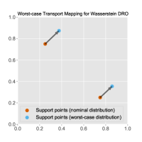
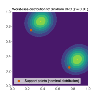
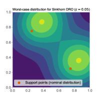
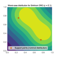
Figure 1: Visualization of worst-case distributions from Wasserstein DRO (left plot) and Sinkhorn DRO models (right three plots) with varying choices of $\epsilon$.

In Figure 1 we visualize the worst-case distributions from Wasserstein/Sinkhorn DRO models. The loss function and transport cost used in this plot follow the setup described in Example 3.7. The Wasserstein ball radius, Sinkhorn ball radius, and entropic regularization value are fine-tuned to ensure that the optimal dual multipliers for all instances equal 5. Notably, the support points of the worst-case distributions from the Wasserstein DRO model correspond to the modes of the continuous worst-case distributions from the Sinkhorn DRO model.

The above demonstrates another difference, or advantage possibly, of Sinkhorn DRO compared with Wasserstein DRO. Indeed, for many practical problems, the underlying distribution is modeled as a continuous distribution. The worst-case distribution for Wasserstein DRO is often finitely supported, raising the concern of whether it hedges against the wrong family of distributions and thus results in suboptimal solutions. The numerical results in Section 5 demonstrate some empirical advantages of Sinkhorn DRO.  $\clubsuit$

Remark 3.4 (Connection with KL-DRO)

Using Jensen’s inequality, we can see that the dual objective function of the Sinkhorn DRO model can be upper-bounded as

$$\lambda\overline{\rho}+\lambda\epsilon\log\left(\mathbb{E}_{x\sim\widehat{\mathbb{P}}}\mathbb{E}_{z\sim\mathbb{Q}_{x,\epsilon}}\left[e^{f(z)/(\lambda\epsilon)}\right]\right),$$

which corresponds to the dual objective for the following KL-divergence DRO [10]

$$\sup_{\mathbb{P}}~{}\left\{\mathbb{E}_{z\sim\mathbb{P}}[f(z)]:~{}D_{\text{KL}}(\mathbb{P}\|\mathbb{P}^{0})\leq\overline{\rho}/\epsilon\right\},$$

where $\mathbb{P}^{0}$ satisfies $\,\mathrm{d}\mathbb{P}^{0}(z)=\mathbb{E}_{x\sim\widehat{\mathbb{P}}}\left[\,\mathrm{d}\mathbb{Q}_{x,\epsilon}(z)\right]$, which can be viewed as a non-parametric kernel density estimation constructed from $\widehat{\mathbb{P}}$. Particularly, when $\widehat{\mathbb{P}}=\frac{1}{n}\sum_{i=1}^{n}\delta_{\hat{x}_{i}},\mathcal{Z}=\mathbb{R}^{d}$ and $c(x,y)=\|x-y\|_{2}^{2}$, $\mathbb{P}^{0}$ is kernel density estimator with Gaussian kernel and bandwidth $\epsilon$:

$$\frac{\,\mathrm{d}\mathbb{P}^{0}(z)}{\,\mathrm{d}z}=\frac{1}{n}\sum_{i=1}^{n}K_{\epsilon}\left(z-x_{i}\right),\quad z\in\mathbb{R}^{d},$$

where $K_{\epsilon}(x)\propto\exp(-\|x\|_{2}^{2}/\epsilon)$ represents the Gaussian kernel. By Lemma 3.11 and divergence inequality [35, Theorem 2.6.3], we can see the Sinkhorn DRO with $\overline{\rho}=0$ is reduced to the following SAA model based on the distribution $\mathbb{P}^{0}$:

$$V=\mathbb{E}_{z\sim\mathbb{P}^{0}}[f(z)]=\mathbb{E}_{x\sim\widehat{\mathbb{P}}}\mathbb{E}_{z\sim\mathbb{Q}_{x,\epsilon}}[f(z)].$$ (4)

In non-parameteric statistics, the optimal bandwidth to minimize the mean-squared-error between the estimated distribution $\mathbb{P}_{0}$ and the underlying true one is at rate $\epsilon=O(n^{-1/(d+4)})$ [56, Theorem 4.2.1]. However, such an optimal choice for the kernel density estimator may not be the optimal choice for optimizing the out-of-sample performance of the Sinkhorn DRO. In our numerical experiments in Section 5, we select $\epsilon$ based on cross-validation.  $\clubsuit$

Remark 3.5 (Connection with Bayesian DRO)

The recent Bayesian DRO framework [106] proposed to solve

$$\mathbb{E}_{x\sim\widehat{\mathbb{P}}}~{}\left[\sup_{\mathbb{P}}~{}\Big{\{}\mathbb{E}_{z\sim\mathbb{P}}[f(z)]:~{}\mathbb{P}\in\mathcal{P}_{x}\Big{\}}\right],$$

where $\widehat{\mathbb{P}}$ is a special posterior distribution constructed from collected observations, and the ambiguity set $\mathcal{P}_{x}$ is typically constructed as a KL-divergence ball, i.e., $\mathcal{P}_{x}:=\{\mathbb{P}:~{}D_{\text{KL}}(\mathbb{P}\|\mathbb{Q}_{x})\leq\eta\}$, with $\mathbb{Q}_{x}$ being the parametric distribution conditioned on $x$. According to [106, Section 2.1.3], a relaxation of the Bayesian DRO dual formulation is given by

$$\inf_{\lambda\geq 0}~{}\left\{\lambda\eta+\lambda\mathbb{E}_{x\sim\widehat{\mathbb{P}}}\Big{[}\log\mathbb{E}_{z\sim\mathbb{Q}_{x}}\left[e^{f(z)/\lambda}\right]\Big{]}\right\}.$$

When specifying the parametric distribution $\mathbb{Q}_{x}$ as the kernel probability distribution in (3) and applying the change-of-variable technique such that $\lambda$ is replaced with $\lambda\epsilon$, this relaxed formulation becomes

$$\inf_{\lambda\geq 0}~{}\left\{\lambda(\eta\epsilon)+\lambda\epsilon\mathbb{E}_{x\sim\widehat{\mathbb{P}}}\Big{[}\log\mathbb{E}_{z\sim\mathbb{Q}_{x}}\left[e^{f(z)/(\lambda\epsilon)}\right]\Big{]}\right\}.$$

In comparison with (Dual), we find the Sinkhorn DRO model can be viewed as a special relaxation formulation of the Bayesian DRO model.  $\clubsuit$

3.3 Examples

In the following, we provide several cases in which our strong dual reformulation (Dual) can be simplified into more tractable formulations.

Example 3.6 (Linear loss)

Suppose that the loss function $f(z)=a^{\mathrm{T}}z$, support $\mathcal{Z}=\mathbb{R}^{d}$, $\nu$ is the corresponding Lebesgue measure, and the transport cost is the Mahalanobis distance, i.e., $c(x,y)=\frac{1}{2}(x-y)^{\mathrm{T}}\Omega(x-y)$, where $\Omega$ is a positive definite matrix. In this case, we have the reference measure $\mathbb{Q}_{x,\epsilon}\sim\mathcal{N}(x,\epsilon\Omega^{-1}).$ As a consequence, the dual problem can be written as

$$V_{\mathrm{D}}=\inf_{\lambda>0}~{}\left\{\lambda\overline{\rho}+\lambda\epsilon\mathbb{E}_{x\sim\widehat{\mathbb{P}}}\Big{[}\Lambda_{x}(\lambda)\Big{]}\right\},$$

where

$$\Lambda_{x}(\lambda)=\log\mathbb{E}_{z\sim\mathcal{N}(x,\epsilon\Omega^{-1})}\left[e^{a^{\top}z/(\lambda\epsilon)}\right]=\frac{a^{\mathrm{T}}x}{\lambda\epsilon}+\frac{a^{\mathrm{T}}\Omega^{-1}a}{2\lambda^{2}\epsilon}.$$

Therefore

$$V_{\mathrm{D}}=a^{\mathrm{T}}\mathbb{E}_{x\sim\widehat{\mathbb{P}}}[x]+\sqrt{2\overline{\rho}}\sqrt{a^{\mathrm{T}}\Omega^{-1}a}:=\mathbb{E}_{x\sim\widehat{\mathbb{P}}}[a^{\mathrm{T}}x]+\sqrt{2\overline{\rho}}\cdot\|a\|_{\Omega^{-1}}.$$

This indicates that the Sinkhorn DRO is equivalent to an empirical risk minimization with norm regularization, and can be solved efficiently using algorithms for the second-order cone program.  $\clubsuit$

Example 3.7 (Quadratic loss)

Consider the example of linear regression with quadratic loss $f_{\theta}(z)=(a^{\mathrm{T}}\theta-b)^{2}$, where $z:=(a,b)$ denotes the predictor-response pair, $\theta\in\mathbb{R}^{d}$ denotes the fixed parameter choice, and $\mathcal{Z}=\mathbb{R}^{d+1}$. Taking $\nu$ as the Lebesgue measure and the transport cost as $c((a,b),(a^{\prime},b^{\prime}))=\frac{1}{2}\|a-a^{\prime}\|_{2}^{2}+\infty|b-b^{\prime}|$. In this case, the dual problem becomes

$$V_{\mathrm{D}}=\mathbb{E}_{z\sim\widehat{\mathbb{P}}}[(a^{\mathrm{T}}\theta-b)^{2}]+\inf_{\lambda>2\|\theta\|_{2}^{2}}~{}\left\{\lambda\overline{\rho}+\frac{\mathbb{E}_{z\sim\widehat{\mathbb{P}}}[(a^{\mathrm{T}}\theta-b)^{2}]}{\frac{1}{2}\lambda\|\theta\|_{2}^{-2}-1}-\frac{\lambda\epsilon}{2}\log\det\left(I-\frac{\theta\theta^{\mathrm{T}}}{\frac{1}{2}\lambda}\right)\right\}.$$

In comparison with the corresponding Wasserstein DRO formulation with radius $\rho$ (see, e.g., [19, Example 4])

$$V_{\mathrm{D}}^{\text{Wasserstein}}=\mathbb{E}_{z\sim\widehat{\mathbb{P}}}[(a^{\mathrm{T}}\theta-b)^{2}]+\inf_{\lambda>2\|\theta\|_{2}^{2}}~{}\left\{\lambda\rho+\frac{\mathbb{E}_{z\sim\widehat{\mathbb{P}}}[(a^{\mathrm{T}}\theta-b)^{2}]}{\frac{1}{2}\lambda\|\theta\|_{2}^{-2}-1}\right\},$$

one can check in this case the Sinkhorn DRO formulation is equivalent to the Wasserstein DRO with log-determinant regularization.  $\clubsuit$

When the support $\mathcal{Z}$ is finite, the following result presents a conic programming reformulation.

Corollary 3.8 (Conic Reformulation for Finite Support)

Suppose that the support contains $L_{\max}$ elements, i.e., $\mathcal{Z}=\{z_{\ell}\}_{\ell=1}^{L_{\max}}$, and the nominal distribution $\widehat{\mathbb{P}}=\frac{1}{n}\sum_{i=1}^{n}\delta_{\hat{x}_{i}}$. If Condition 1 holds and $\overline{\rho}\geq 0$, the dual problem (Dual) can be formulated as the following conic optimization:

$$V_{\mathrm{D}}=\min_{\begin{subarray}{c}\lambda\geq 0,s\in\mathbb{R}^{n},\\ a\in\mathbb{R}^{n\times L}\end{subarray}} \quad\lambda\overline{\rho}+\frac{1}{n}\sum_{i=1}^{n}s_{i}$$ (5)

s.t. $$\quad\lambda\epsilon\geq\sum_{\ell=1}^{L_{\max}}q_{i,\ell}a_{i,\ell},i\in[n],$$

$$\quad(\lambda\epsilon,a_{i,\ell},f(z_{\ell})-s_{i})\in\mathcal{K}_{\exp},i\in[n],\ell\in[L].$$

where $q_{i,\ell}:=\Pr_{z\sim\mathbb{Q}_{\hat{x}_{i},\epsilon}}\{z=z_{\ell}\}$, with the distribution $\mathbb{Q}_{\hat{x}_{i},\epsilon}$ defined in (3), and $\mathcal{K}_{\exp}$ denotes the exponential cone $\mathcal{K}_{\exp}=\left\{(\nu,\lambda,\delta)\in\mathbb{R}_{+}\times\mathbb{R}_{+}\times\mathbb{R}:~{}\exp(\delta/\nu)\leq\lambda/\nu\right\}$.

Problem (5) is a convex program that minimizes a linear function with respect to linear and conic constraints, which can be solved using interior point algorithms [83, 118]. We will develop an efficient first-order optimization algorithm in Section 4 that is able to solve a more general problem (without a finite support).

3.4 Proof of Theorem 3.1

In this subsection, we present a sketch of the proof for Theorem 3.1. We begin with the weak duality result in Lemma 3.9, which can be shown by applying the Lagrangian weak duality.

Lemma 3.9 (Weak Duality)

Under Assumption 3.1, it holds that

$$V\leq\inf_{\lambda\geq 0}\;\bigg{\{}\lambda\rho+\lambda\epsilon\;\mathbb{E}_{x\sim\widehat{\mathbb{P}}}\Big{[}\log\mathbb{E}_{z\sim\nu}\big{[}e^{(f(z)-\lambda c(x,z))/(\lambda\epsilon)}\big{]}\Big{]}\bigg{\}}=V_{\mathrm{D}}.$$

Proof 3.10

Proof of Lemma 3.9. Based on Definition 2.1 of Sinkhorn distance, we reformulate $V$ as

$$V =\sup_{\gamma\in\mathcal{P}(\mathcal{Z}\times\mathcal{Z}):\mathrm{Proj}_{1\#}\gamma=\widehat{\mathbb{P}}}\left\{\mathbb{E}_{z\sim\mathbb{P}}[f(z)]:\mathbb{E}_{(x,z)\sim\gamma}\left[c(x,z)+\epsilon\log\left(\frac{\,\mathrm{d}\gamma(x,z)}{\,\mathrm{d}\widehat{\mathbb{P}}(x)\,\mathrm{d}\nu(z)}\right)\right]\leq\rho\right\}.$$

By the law of total expectation, the constraint is equivalent to

$$\mathbb{E}_{x\sim\widehat{\mathbb{P}}}\mathbb{E}_{z\sim\gamma_{x}}\left[c(x,z)+\epsilon\log\left(\frac{\,\mathrm{d}\gamma_{x}(z)}{\,\mathrm{d}\nu(z)}\right)\right]\leq\rho,$$

and the primal problem is equivalent to

$$V=\sup_{\{\gamma_{x}\}_{x\in\mathrm{supp}\,\widehat{\mathbb{P}}}\subset\mathcal{P}(\mathcal{Z})}\left\{\mathbb{E}_{x\sim\widehat{\mathbb{P}}}\mathbb{E}_{z\sim\gamma_{x}}[f(z)]:\ \mathbb{E}_{x\sim\widehat{\mathbb{P}}}\mathbb{E}_{z\sim\gamma_{x}}\left[c(x,z)+\epsilon\log\left(\frac{\,\mathrm{d}\gamma_{x}(z)}{\,\mathrm{d}\nu(z)}\right)\right]\leq\rho\right\}.$$ (6)

Introducing the Lagrange multiplier $\lambda$ associated to the constraint, we reformulate $V$ as

$$V=\sup_{\{\gamma_{x}\}_{x\in\mathrm{supp}\,\widehat{\mathbb{P}}}\subset\mathcal{P}(\mathcal{Z})}~{}\left\{\inf_{\lambda\geq 0}~{}\left\{\lambda\rho+\mathbb{E}_{x\sim\widehat{\mathbb{P}}}\mathbb{E}_{z\sim\gamma_{x}}\left[f(z)-\lambda c(x,z)-\lambda\epsilon\log\left(\frac{\,\mathrm{d}\gamma_{x}(z)}{\,\mathrm{d}\nu(z)}\right)\right]\right\}\right\}.$$

Interchanging the order of the supremum and infimum operators, we have that

$$V\leq\inf_{\lambda\geq 0}~{}\left\{\lambda\rho+\sup_{\{\gamma_{x}\}_{x\in\mathrm{supp}\,\widehat{\mathbb{P}}}\subset\mathcal{P}(\mathcal{Z})}\left\{\mathbb{E}_{x\sim\widehat{\mathbb{P}}}\mathbb{E}_{z\sim\gamma_{x}}\left[f(z)-\lambda c(x,z)-\lambda\epsilon\log\left(\frac{\,\mathrm{d}\gamma_{x}(z)}{\,\mathrm{d}\nu(z)}\right)\right]\right\}\right\}.$$

Since the optimization over $\{\gamma_{x}\}_{x}$ is separable for each $x$, by defining

$$v_{x}(\lambda) :=\sup_{\gamma_{x}\in\mathcal{P}(\mathcal{Z})}~{}\left\{\mathbb{E}_{z\sim\gamma_{x}}\left[f(z)-\lambda c(x,z)-\lambda\epsilon\log\left(\frac{\,\mathrm{d}\gamma_{x}(z)}{\,\mathrm{d}\nu(z)}\right)\right]\right\},$$

and swap the supremum and the integration, we obtain

$$V\leq\inf_{\lambda\geq 0}~{}\left\{\lambda\rho+\mathbb{E}_{x\sim\widehat{\mathbb{P}}}\Big{[}v_{x}(\lambda)\Big{]}\right\}.$$ (7)

Since $v_{x}(\lambda)$ is an entropic regularized linear optimization, by Lemma 11.1, when there exists $\lambda>0$ such that Condition 1 is satisfied, it holds that $\mathbb{E}_{z\sim\nu}\big{[}e^{(f(z)-\lambda c(x,z))/(\lambda\epsilon)}\big{]}<\infty$, $v_{x}(\lambda)$ is measurable with respect to $x\sim\widehat{\mathbb{P}}$ and

$$v_{x}(\lambda)=\lambda\epsilon\log\mathbb{E}_{z\sim\nu}\big{[}e^{(f(z)-\lambda c(x,z))/(\lambda\epsilon)}\big{]}<\infty.$$

In this case, the desired result holds. If for any $\lambda>0$,

$$\widehat{\mathbb{P}}\left\{x:~{}\mathbb{E}_{z\sim\mathbb{Q}_{x,\epsilon}}\left[e^{f(z)/(\lambda\epsilon)}\right]=\infty\right\}=\widehat{\mathbb{P}}\left\{x:~{}\mathbb{E}_{z\sim\nu}\big{[}e^{(f(z)-\lambda c(x,z))/(\lambda\epsilon)}\big{]}=\infty\right\}>0,$$

then intermediately we obtain

$$V\leq\inf_{\lambda\geq 0}\;\bigg{\{}\lambda\rho+\lambda\epsilon\;\mathbb{E}_{x\sim\widehat{\mathbb{P}}}\Big{[}\log\mathbb{E}_{z\sim\nu}\big{[}e^{(f(z)-\lambda c(x,z))/(\lambda\epsilon)}\big{]}\Big{]}\bigg{\}}=\infty,$$

and the weak duality still holds.  $\square$

Next, we show the feasibility result in Theorem 3.1(I). The key observation is that the primal problem (Primal) can be reformulated as a generalized KL-divergence DRO problem.

Lemma 3.11 (Reformulation of (Primal))

Under Assumption 3.1, it holds that

$$V=\sup_{\{\gamma_{x}\}_{x\in\mathrm{supp}\,\widehat{\mathbb{P}}}\subset\mathcal{P}(\mathcal{Z})}\left\{\mathbb{E}_{x\sim\widehat{\mathbb{P}}}\mathbb{E}_{z\sim\gamma_{x}}[f(z)]:\ \epsilon\mathbb{E}_{x\sim\widehat{\mathbb{P}}}\mathbb{E}_{z\sim\gamma_{x}}\left[\log\left(\frac{\,\mathrm{d}\gamma_{x}(z)}{\,\mathrm{d}\mathbb{Q}_{x,\epsilon}(z)}\right)\right]\leq\overline{\rho}\right\}.$$

Due to Lemma 3.11, Theorem 3.1(I) holds because of the non-negativity of KL-divergence.

Finally, we develop the strong duality. In the following, we provide the proof of the first part of Theorem 3.1(III) for the most representative case where $\overline{\rho}>0$, the dual minimizer $\lambda^{*}$ exists with $\lambda^{*}>0$, and Condition 1 holds. Proofs of other cases are moved in Appendix 11. Below we develop the optimality condition when the dual minimizer $\lambda^{*}>0$ in Lemma 3.12, by simply setting the derivative of the dual objective function to be zero.

Lemma 3.12 (First-order Optimality Condition when $\lambda^{*}>0$)

Suppose $\overline{\rho}>0$ and Condition 1 is satisfied, and assume further that the dual minimizer $\lambda^{*}>0$, then $\lambda^{*}$ satisfies

$$\overline{\rho}+\epsilon\mathbb{E}_{x\sim\widehat{\mathbb{P}}}\left[\log\mathbb{E}_{z\sim\mathbb{Q}_{x,\epsilon}}\left[e^{f(z)/(\lambda^{*}\epsilon)}\right]\right]=\frac{1}{\lambda^{*}}\mathbb{E}_{x\sim\widehat{\mathbb{P}}}\left[\frac{\mathbb{E}_{z\sim\nu}\left[e^{(f(z)-\lambda^{*}c(x,z))/(\lambda^{*}\epsilon)}f(z)\right]}{\mathbb{E}_{z\sim\nu}\left[e^{(f(z)-\lambda^{*}c(x,z))/(\lambda^{*}\epsilon)}\right]}\right].$$ (8)

We prove the strong duality by constructing the worst-case distribution.

Proof 3.13

Proof of Theorem 3.1(III) for the case where Condition 1 holds and $\overline{\rho}>0,\lambda^{*}>0$. We take the transport mapping $\gamma_{*}$ such that

$$\frac{\,\mathrm{d}\gamma_{*}(x,z)}{\,\mathrm{d}\widehat{\mathbb{P}}(x)\,\mathrm{d}\nu(z)}=\alpha_{x}\cdot\exp\Big{(}\big{(}f(z)-\lambda^{\ast}c(x,z)\big{)}/(\lambda^{\ast}\epsilon)\Big{)},$$

and $\alpha_{x}:=\left(\mathbb{E}_{z\sim\nu}\left[e^{(f(z)-\lambda^{\ast}c(x,z))/(\lambda^{\ast}\epsilon)}\right]\right)^{-1}$ is a normalizing constant such that $\mathrm{Proj}_{1\#}\gamma_{*}=\widehat{\mathbb{P}}$. Also define the primal (approximate) optimal distribution $\mathbb{P}_{\ast}:=\mathrm{Proj}_{2\#}\gamma_{*}.$ Recall the expression of the Sinkhorn distance in Definition 2.1, one can verify that

$$\hphantom{=}\mathcal{W}_{\epsilon}(\widehat{\mathbb{P}},\mathbb{P}_{\ast})=\inf_{\gamma\in\Gamma(\widehat{\mathbb{P}},\mathbb{P}_{\ast})}~{}\left\{\mathbb{E}_{(x,z)\sim\gamma}\left[c(x,z)+\epsilon\log\left(\frac{\,\mathrm{d}\gamma(x,z)}{\,\mathrm{d}\widehat{\mathbb{P}}(x)\,\mathrm{d}\nu(z)}\right)\right]\right\}$$

$$=\inf_{\gamma\in\Gamma(\widehat{\mathbb{P}},\mathbb{P}_{\ast})}~{}\left\{\mathbb{E}_{(x,z)\sim\gamma}\left[\epsilon\log\left(\frac{e^{c(x,z)/\epsilon}\,\mathrm{d}\gamma(x,z)}{\,\mathrm{d}\widehat{\mathbb{P}}(x)\,\mathrm{d}\nu(z)}\right)\right]\right\}$$

$$\leq\mathbb{E}_{(x,z)\sim\gamma_{*}}\left[\epsilon\log\left(\frac{e^{c(x,z)/\epsilon}\,\mathrm{d}\gamma_{*}(x,z)}{\,\mathrm{d}\widehat{\mathbb{P}}(x)\,\mathrm{d}\nu(z)}\right)\right]=\mathbb{E}_{(x,z)\sim\gamma_{*}}\left\{\frac{1}{\lambda^{*}}f(z)+\epsilon\log(\alpha_{x})\right\}$$

$$=\frac{1}{\lambda^{*}}\mathbb{E}_{x\sim\widehat{\mathbb{P}}}\left[\frac{\mathbb{E}_{z\sim\nu}\left[e^{(f(z)-\lambda^{*}c(x,z))/(\lambda^{*}\epsilon)}f(z)\right]}{\mathbb{E}_{z\sim\nu}\left[e^{(f(z)-\lambda^{*}c(x,z))/(\lambda^{*}\epsilon)}\right]}\right]-\epsilon\mathbb{E}_{x\sim\widehat{\mathbb{P}}}\left[\log\mathbb{E}_{z\sim\nu}\left[e^{(f(z)-\lambda^{\ast}c(x,z))/(\lambda^{\ast}\epsilon)}\right]\right]$$

where the inequality relation is because $\gamma_{*}$ is a feasible solution in $\Gamma(\widehat{\mathbb{P}},\mathbb{P}_{\ast})$, and the last two relations are by substituting the expression of $\gamma_{*}$. Since $\overline{\rho}>0$ and the dual minimizer $\lambda^{*}>0$, the optimality condition in (8) holds, which implies that $\mathcal{W}_{\epsilon}(\widehat{\mathbb{P}},\mathbb{P}_{\ast})\leq\rho$, i.e., the distribution $\mathbb{P}_{\ast}$ is primal feasible for the problem (Primal). Moreover, we can see that the primal optimal value is lower bounded by the dual optimal value:

$$V~{}\geq ~{}\mathbb{E}_{\mathbb{P}_{\ast}}[f(z)]=\mathbb{E}_{(x,z)\sim\gamma_{\ast}}[f(z)]$$

$$= \mathbb{E}_{x\sim\widehat{\mathbb{P}}}\mathbb{E}_{z\sim\nu}\left[f(z)\left(\frac{\,\mathrm{d}\gamma_{*}(x,z)}{\,\mathrm{d}\widehat{\mathbb{P}}(x)\,\mathrm{d}\nu(z)}\right)\right]=\mathbb{E}_{x\sim\widehat{\mathbb{P}}}\left[\frac{\mathbb{E}_{z\sim\nu}\left[e^{(f(z)-\lambda^{*}c(x,z))/(\lambda^{*}\epsilon)}f(z)\right]}{\mathbb{E}_{z\sim\nu}\left[e^{(f(z)-\lambda^{*}c(x,z))/(\lambda^{*}\epsilon)}\right]}\right]$$

$$= \lambda^{*}\left(\overline{\rho}+\epsilon\mathbb{E}_{x\sim\widehat{\mathbb{P}}}\left[\log\mathbb{E}_{z\sim\mathbb{Q}_{x,\epsilon}}\left[e^{f(z)/(\lambda^{*}\epsilon)}\right]\right]\right)=V_{\mathrm{D}},$$

where the third equality is by substituting the expression of $\gamma_{\ast}$, and the last equality is based on the optimality condition in (8). This, together with the weak duality, completes the proof.  $\square$

4 Efficient First-order Algorithm for Sinkhorn Robust Optimization

Consider the Sinkhorn robust optimization problem

$$\inf_{\theta\in\Theta}\sup_{\mathbb{P}\in\mathbb{B}_{\rho,\epsilon}(\widehat{\mathbb{P}})}~{}\mathbb{E}_{z\sim\mathbb{P}}[f_{\theta}(z)].$$ (9)

Here the feasible set $\Theta\subseteq\mathbb{R}^{d_{\theta}}$ is closed and convex containing all possible candidates of decision vector $\theta$, and the Sinkhorn uncertainty set is centered around a given nominal distribution $\widehat{\mathbb{P}}$. Based on our strong dual expression (Dual), we reformulate (9) as

$$\inf_{\lambda\geq 0}~{}\left\{\lambda\overline{\rho}+\inf_{\theta\in\Theta}~{}\mathbb{E}_{x\sim\widehat{\mathbb{P}}}\bigg{[}\lambda\epsilon\log\mathbb{E}_{z\sim\mathbb{Q}_{x,\epsilon}}\left[e^{f_{\theta}(z)/(\lambda\epsilon)}\right]\bigg{]}\right\},$$ (D)

where the constant $\overline{\rho}$ and the distribution $\mathbb{Q}_{x,\epsilon}$ are defined in (2) and (3), respectively. In Example 3.6 and 3.7, we have seen special instances of (D) where we can get closed-form expressions for the above integration. For general loss functions when a closed-form expression is not available, we resort to an algorithmic approach, which is the main development in this section.

A typical and efficient approach for solving a stochastic optimization problem is the stochastic gradient descent method such as stochastic mirror descent [82]. However, unlike many other stochastic optimization problems, one salient feature of (D) is that the objective function of (10) involves a nonlinear transformation of the expectation. Consequently, based on a batch of simulated samples from $\mathbb{Q}_{x,\epsilon}$, an unbiased gradient estimate could be challenging to obtain. In Section 4.1, we will present a biased stochastic mirror descent algorithm to solve this problem. By properly balancing their bias and second-order moment trade-off in the biased gradient estimator, our algorithm can efficiently find a near-optimal decision of (10), as we will analyze in Section 4.2.

4.1 Main Algorithm

Define the objective value of the outer minimization in (D) as

$$F^{*}(\lambda):=\lambda\overline{\rho}+\inf_{\theta\in\Theta}\left\{\mathbb{E}_{x\sim\widehat{\mathbb{P}}}\bigg{[}\lambda\epsilon\log\mathbb{E}_{z\sim\mathbb{Q}_{x,\epsilon}}\left[e^{f_{\theta}(z)/(\lambda\epsilon)}\right]\bigg{]}\right\}.$$ (10)

We first present a Biased Stochastic Mirror Descent (BSMD) algorithm that solves the minimization over the decisions $\theta$ for a given Lagrangian multiplier $\lambda$ in Section 4.1.1. Next, in Section 4.1.2 we present a bisection search algorithm for finding the optimal Lagrangian multiplier.

4.1.1 Biased Stochastic Mirror Descent

Since the multiplier $\lambda$ is fixed in (10), we omit the dependence of $\lambda$ when defining objective or gradient terms in this subsection and set

$$F(\theta):=\mathbb{E}_{x\sim\widehat{\mathbb{P}}}\bigg{[}\lambda\epsilon\log\mathbb{E}_{z\sim\mathbb{Q}_{x,\epsilon}}\left[e^{f_{\theta}(z)/(\lambda\epsilon)}\right]\bigg{]}.$$ (11)

We first introduce several notations that are standard in the mirror descent algorithm. Let $\omega:~{}\Theta\to\mathbb{R}$ be a distance generating function that is continuously differentiable and $\kappa$-strongly convex on $\Theta$ with respect to norm $\|\cdot\|$. This induces the Bregman divergence $D_{\omega}(\theta,\theta^{\prime}):~{}\Theta\times\Theta\to\mathbb{R}_{+}$:

$$D_{\omega}(\theta,\theta^{\prime})=\omega(\theta^{\prime})-\omega(\theta)-\langle\nabla\omega(\theta),\theta^{\prime}-\theta\rangle.$$

We define the prox-mapping $\mathrm{Prox}:~{}\mathbb{R}^{d_{\theta}}\to\Theta$ as

$$\mathrm{Prox}_{\theta}(y)=\argmin_{\theta^{\prime}\in\Theta}\big{\{}\langle y,\theta^{\prime}-\theta\rangle+D_{\omega}(\theta,\theta^{\prime})\big{\}}.$$

With these notations in hand, we present our algorithm in Algorithm 1.

Algorithm 1 BSMD for finding the optimal solution of (10) while fixing $\lambda$

0:   Maximal iteration $T_{\text{in}}$, constant step size $\gamma$, initial guess $\theta_{1}$, fixed multiplier $\lambda$.

1:  for $t=0,1,\ldots,T_{\text{in}}-1$ do

2:     Formulate a (biased) gradient estimate $v(\theta_{t})$ of $F(\theta_{t})$ using (13).

3:      Update $\theta_{t+1}=\mathrm{Prox}_{\theta_{t}}\big{(}\gamma v(\theta_{t})\big{)}$.

4:  end forOutput the estimate of optimal solution $\widehat{\theta}_{i}=\frac{1}{T_{\mathrm{in}}}\sum_{t=1}^{T_{\mathrm{in}}}\theta_{t}$.

Algorithm 1 iteratively obtains a biased stochastic gradient estimate and performs a proximal gradient update. In Step 2 of Algorithm 1, we adopt the idea of multi-level Monte-Carlo (MLMC) simulation [60] to generate biased gradient estimates with controlled bias. To this end, we first construct a function $F^{\ell}(\theta)$ that approximate the original objective function $F(\theta)$ with $\mathcal{O}(2^{-\ell})$-gap:

$$F^{\ell}(\theta)=\mathbb{E}_{x^{\ell}\sim\widehat{\mathbb{P}}}~{}\mathbb{E}_{\{z^{\ell}_{j}\}_{j\in[2^{\ell}]}\sim\mathbb{Q}_{x^{\ell},\epsilon}}\bigg{[}\lambda\epsilon\log\Big{(}\frac{1}{2^{\ell}}\sum_{j\in[2^{\ell}]}e^{f_{\theta}(z^{\ell}_{j})/(\lambda\epsilon)}\Big{)}\bigg{]},$$ (12)

where the random variable $x^{\ell}$ follows distribution $\widehat{\mathbb{P}}$, and given a realization of $x^{\ell}$, $\{z^{\ell}_{j}\}_{j\in[2^{\ell}]}$ are independent and identically distributed samples from $\mathbb{Q}_{x^{\ell},\epsilon}$. Unlike the original objective $F(\theta)$, unbiased gradient estimators of its approximation $F^{\ell}(\theta)$ can be easily obtained. Denote by $\zeta^{\ell}=(x^{\ell},\{z^{\ell}_{j}\}_{j\in[2^{\ell}]})$ the collection of random sampling parameters, and

$$U_{n_{1}:n_{2}}(\theta,\zeta^{\ell}):=\lambda\epsilon\log\Big{(}\frac{1}{n_{2}-n_{1}+1}\sum_{j\in[n_{1}:n_{2}]}e^{f_{\theta}(z^{\ell}_{j})/(\lambda\epsilon)}\Big{)}.$$

For a fixed parameter $\theta$, we define

$$g^{\ell}(\theta,\zeta^{\ell}) :=\nabla_{\theta}U_{1:2^{\ell}}(\theta,\zeta^{\ell}),$$

$$G^{\ell}(\theta,\zeta^{\ell}) :=\nabla_{\theta}\left[U_{1:2^{\ell}}(\theta,\zeta^{\ell})-\frac{1}{2}U_{1:2^{\ell-1}}(\theta,\zeta^{\ell})-\frac{1}{2}U_{2^{\ell-1}+1:2^{\ell}}(\theta,\zeta^{\ell})\right].$$

The random vector $g^{\ell}(\theta,\zeta^{\ell})$ is an unbiased estimator of $\nabla F^{\ell}(\theta)$, while the vector $G^{\ell}(\theta,\zeta^{\ell})$ is an unbiased estimator of $\nabla F^{\ell}(\theta)-\nabla F^{\ell-1}(\theta)$. The latter facilitates the reduction of second-order moment of the gradient estimator thanks to common random numbers. More specifically, we list the following choices of gradient estimators at a point $\theta$:

– Stochastic Gradient (SG) Estimator: Get $$n^{\mathrm{o}}_{L} \{g^{L}(\theta,\zeta^{L}_{i})\}_{i=1}^{n^{\mathrm{o}}_{L}} \{\zeta^{L}_{i}\}_{i} \zeta^{\ell}$$ random vectors , where are i.i.d. copies of . Construct

$$v^{\text{SG}}(\theta)=\frac{1}{n^{\mathrm{o}}_{L}}\sum_{i=1}^{n^{\mathrm{o}}_{L}}g^{L}(\theta,\zeta^{L}_{i}).$$ (13a)

– Randomized Truncation MLMC (RT-MLMC) Estimator [22]: Sample $$n^{\mathrm{o}}_{L} \iota_{1},\ldots,\iota_{n^{\mathrm{o}}_{L}} \mathbb{P}(\iota=\ell)=\frac{2^{-\ell}}{2-2^{-L}},\ell=0,1,\ldots,L$$ random levels i.i.d. from a distribution . Construct

$$v^{\text{RT-MLMC}}(\theta)=\frac{1}{n^{\mathrm{o}}_{L}}\sum_{i=1}^{n^{\mathrm{o}}_{L}}\frac{1}{\mathbb{P}(\iota=\iota_{i})}G^{\iota_{i}}(\theta,\zeta^{\iota_{i}}).$$ (13b)

Remark 4.1 (Sampling from $\mathbb{Q}_{x,\epsilon}$)

In many cases, generating samples from $\mathbb{Q}_{x,\epsilon}$ is easy. For example, when the transport cost $c(\cdot,\cdot)=\frac{1}{2}\|\cdot-\cdot\|_{2}^{2}$ and $\mathcal{Z}=\mathbb{R}^{d}$, then the distribution $\mathbb{Q}_{x,\epsilon}$ becomes a Gaussian distribution $\mathcal{N}(x,\epsilon I_{d})$. When the transport cost $c(\cdot,\cdot)$ is decomposable in each coordinate, we can apply the acceptance-rejection method [5] to generate samples in each coordinate independently, the complexity of which only increases linearly in the data dimension. When the transport cost $c(x,y)=\frac{1}{q}\|x-y\|_{p}^{q}$, the complexity of sampling based on Lagenvin Monte Carlo method for obtaining a $\tau$-close sample point is $\mathcal{O}(d/\tau)$. See the detailed algorithm of sampling in Appendix 13.2.  $\clubsuit$

4.1.2 Bisection Search

Bisection search requires an oracle that produces an objective estimator of (D). We describe it in Algorithm 2. For a fixed multiplier $\lambda$, it solves problem (10) using Algorithm 1 and then estimates the corresponding objective value. It has $m$ repetitions, whose value will be determined later in Section 4.2 to achieve the best sample complexity.

Algorithm 2 Evaluating the objective value of (D)

0:   Fixed multiplier $\lambda$, error tolerance $\delta$, batch size $m$.

1:  for $j=1,2,\ldots,m$ do

2:      Obtain a $\delta$-optimal solution $\widehat{\theta}_{j}$ of problem (10) using Algorithm 1.

3:      Estimate the objective in (11) using RT-MLMC estimator in (13b), denoted as $\widehat{F}(\widehat{\theta}_{j};\lambda)$ .

4:  end forOutput $\widehat{F}^{*}(\lambda):=\lambda\overline{\rho}+\min_{j\in[m]}~{}\widehat{F}(\widehat{\theta}_{j};\lambda)$.

Below, we present the RT-MLMC-based objective estimator of (11) that is used in Step 3 of Algorithm 2. For notational simplicity, we define

$$A^{\ell}(\theta,\zeta^{\ell}) =U_{1:2^{\ell}}(\theta,\zeta^{\ell})-\frac{1}{2}U_{1:2^{\ell-1}}(\theta,\zeta^{\ell})-\frac{1}{2}U_{2^{\ell-1}+1:2^{\ell}}(\theta,\zeta^{\ell}).$$

It is worth noting that [59, Theorem 4.1] proposed and analyzed the SG estimator for estimating the objective value of CSO problems. Its sample complexity is $\mathcal{O}(\delta^{-3})$, while our proposed RT-MLMC-based estimator has improved sample complexity $\widetilde{\mathcal{O}}(\delta^{-2})$ (see a formal statement in Proposition 4.4).

– Randomized Truncation MLMC (RT-MLMC) Estimator: Sample $n^{\mathrm{o}}_{L}$ random levels $\iota_{1},\ldots,\iota_{n^{\mathrm{o}}_{L}}$ i.i.d. from a distribution $\mathbb{P}(\iota=\ell)=\frac{2^{-\ell}}{2-2^{-L}},\ell=0,1,\ldots,L$. Construct

$$\widehat{F}^{\text{RT-MLMC}}(\theta)=\frac{1}{n^{\mathrm{o}}_{L}}\sum_{i=1}^{n^{\mathrm{o}}_{L}}\frac{1}{\mathbb{P}(\iota=\iota_{i})}A^{\iota_{i}}(\theta,\zeta^{\iota_{i}}).$$ (14)

Given an inexact objective oracle of (D), we use bisection search to find a near-optimal multiplier in (D); see Algorithm 3.

Algorithm 3 Bisection search for finding the optimal multiplier of (D)

0:   Interval $[\lambda_{l},\lambda_{u}]$, maximum outer iterations $T_{\mathrm{out}}$

1:   $\lambda^{(0)}=\lambda_{l}$, $\chi_{l}^{(0)}=\lambda_{l},\chi_{u}^{(0)}=\lambda_{u}$.

2:  for $t=1,\ldots,T_{\text{out}}$ do

3:      Update $\beta_{l}^{(t)}=\frac{1}{3}\big{[}2\chi_{l}^{(t-1)}+\chi_{u}^{(t-1)}\big{]}$ and $\beta_{u}^{(t)}=\frac{1}{3}\big{[}\chi_{l}^{(t-1)}+2\chi_{u}^{(t-1)}\big{]}$.

4:      Query Algorithm 2 to obtain objective estimators of $\beta_{l}^{(t)},\beta_{u}^{(t)}$, denoted as $\widehat{F}^{*}(\beta_{l}^{(t)}),\widehat{F}^{*}(\beta_{u}^{(t)})$, respectively.

5:     if $\widehat{F}^{*}(\beta_{l}^{(t)})\leq\widehat{F}^{*}(\beta_{u}^{(t)})$ then

6:        Update $(\chi_{l}^{(t)},\chi_{u}^{(t)})=(\chi_{l}^{(t-1)},\beta_{u}^{(t)})$.

7:         if $\widehat{F}^{*}(\beta_{l}^{(t)})\leq\widehat{F}^{*}(\lambda^{(t-1)})$, update $\lambda^{(t)}=\beta_{l}^{(t)}$; else update $\lambda^{(t)}=\lambda^{(t-1)}$.

8:     else

9:        Update $(\chi_{l}^{(t)},\chi_{u}^{(t)})=(\beta_{l}^{(t)},\chi_{u}^{(t-1)})$.

10:         if $\widehat{F}^{*}(\beta_{u}^{(t)})\leq\widehat{F}^{*}(\lambda^{(t-1)})$, update $\lambda^{(t)}=\beta_{u}^{(t)}$; else update $\lambda^{(t)}=\lambda^{(t-1)}$.

11:     end if

12:  end forOutput $\lambda^{(T_{out})}$.

Another approach to solving (D) is to jointly optimize $(\lambda,\theta)$. However, as mentioned in [79], the variance of the gradient estimate of the objective function with respect to $\lambda$ becomes unstable when $\lambda$ is small. Consequently, in our algorithm, we have developed a bisection method to update $\lambda$ instead.

We also remark that, as a practical alternative, one can solve (10) using Algorithm 1 alone and tune the hyperparameter $\lambda$, as tuning the radius $\overline{\rho}$ is equivalent to tuning the Lagrangian multiplier $\lambda$ in (10). This corresponds to the Sinkhorn robust learning problem with a soft Sinkhorn constraint.

4.2 Convergence Analysis

In this subsection, we analyze the convergence properties of the proposed algorithms. We begin with the following standard assumptions on the loss function $f_{\theta}$:

1. (Convexity): The loss function $f_{\theta}(z)$ is convex in $\theta$.

2. (Boundedness): The loss function $f_{\theta}(z)$ satisfies $0\leq f_{\theta}(z)\leq B$ for any $\theta\in\Theta$ and $z\in\mathcal{Z}$.

3. (Lipschitz Continuity): For fixed $z$ and $\theta_{1},\theta_{2}$, it holds that $|f_{\theta_{1}}(z)-f_{\theta_{2}}(z)|\leq L_{f}\|\theta_{1}-\theta_{2}\|_{2}$.

In the following analysis, the sample complexity of an algorithm is defined as the number of samples $(x,z)$, where $x\sim\widehat{\mathbb{P}}$ and $z\sim\mathbb{Q}_{x}$, in total used by the algorithm, and the storage cost is defined the number of samples stored in the memory.

4.2.1 Complexity of Biased Stochastic Mirror Descent

In this part, we discuss the complexity of Algorithm 1. We say $\theta$ is a $\delta$-optimal solution if $\mathbb{E}[F(\theta)]-F(\theta^{*})\leq\delta$, where $\theta^{*}$ is the optimal solution of (10). By properly tuning hyper-parameters to balance the trade-off between bias and second-order moment of the gradient estimate, we establish its performance guarantees in Theorem 4.2. The explicit constants and detailed proof can be found in Appendix 13.

Theorem 4.2

Under Assumptions 4.2(I), 4.2(II), and 4.2(III), with properly chosen hyper-parameters as in Table 2, the following results hold:

1. The sample complexity of Algorithm 1 using SG scheme (13a) to obtain a $\delta$-optimal solution is $\mathcal{O}(\delta^{-3})$, with storage cost $\mathcal{O}(\delta^{-1})$.

2. The sample complexity of Algorithm 1 using RT-MLMC scheme (13b) to obtain a $\delta$-optimal solution is $\widetilde{\mathcal{O}}(\delta^{-2})$, with storage cost $\widetilde{\mathcal{O}}(1)$.

Table 2: Hyper-parameters, sample complexity (Samp.), and storage cost (Stor.) of Algorithm 1.

Estimators	Hyper-parameters	Samp./Stor.
SG	$L=\mathcal{O}(\log\frac{1}{\delta}),\quad T_{\mathrm{in}}=\mathcal{O}(\delta^{-2})$	$\mbox{Samp.}=\mathcal{O}(T_{\mathrm{in}}n^{\mathrm{o}}_{L}2^{L})=\mathcal{O}(\delta^{-3})$
	$n^{\mathrm{o}}_{L}=\mathcal{O}(1),\quad\gamma=\mathcal{O}(\delta)$	$\mbox{Stor.}=\mathcal{O}(n^{\mathrm{o}}_{L}2^{L})=\mathcal{O}(\delta^{-1})$
RT-MLMC	$L=\mathcal{O}(\log\frac{1}{\delta}),\quad T_{\mathrm{in}}=\widetilde{\mathcal{O}}(\delta^{-2})$	$\mbox{Samp.}=\mathcal{O}(T_{\mathrm{in}}(n^{\mathrm{o}}_{L}L))=\widetilde{\mathcal{O}}(\delta^{-2})$
	$n^{\mathrm{o}}_{L}=\mathcal{O}(1),\quad\gamma=\widetilde{\mathcal{O}}(\delta)$	$\mbox{Stor.}=\mathcal{O}(n^{\mathrm{o}}_{L}L)=\widetilde{\mathcal{O}}(1)$

Theorem 4.2 indicates that the sample complexity of BSMD using SG scheme for solving (10) is $\mathcal{O}(\delta^{-3})$, and can be further improved to $\widetilde{\mathcal{O}}(\delta^{-2})$ using the RT-MLMC gradient estimator. This complexity is near-optimal, which matches the information-theoretic lower bound for general convex optimization problems [82]. Besides, using RT-MLMC gradient estimator instead of SG estimator achieves cheaper storage cost of $\widetilde{\mathcal{O}}(1)$, which is nearly error tolerance-independent.

We remark that the problem (10) can be viewed as a special conditional stochastic optimization (CSO) problem [59, 61, 60]. In contrast to the previous state-of-the-art [60], which focused solely on unconstrained optimization where stochastic gradient descent is applied, we consider a constrained optimization on $\theta$ where stochastic mirror descent is applied. Furthermore, our approach achieves the near-optimal sample complexity for both smooth and nonsmooth loss functions, distinguishing it from [61, Theorem 3.2], which shows sample complexity of $O(\delta^{-4})$ for nonsmooth loss functions. Our result can be easily extended to general CSO problems with general convex loss functions which, to the best of our knowledge, is the first algorithm for such problems with provably near-optimal sample complexity.

Remark 4.3 (Comparison with Biased Sample Average Approximation)

Another way to solve (10) is to approximate the objective using finite samples for both expectations. This leads to a biased sample estimate, called Biased Sample Average Approximation (BSAA). Applying [59, Corollary 4.2], it can be shown that the total sample complexity and storage cost for BSAA are both $\widetilde{\mathcal{O}}(\delta^{-3})$ for convex, bounded and Lipschitz loss functions (see formal statement in Appendix 13.3). Our proposed BSMD with the RT-MLMC-based gradient estimator has smaller sample complexity and storage cost. Also, the BSAA method still requires computing the optimal solution of the approximated optimization problem as the output. Hence, it typically takes considerably less time and memory to run the BSMD step rather than solving for the BSAA formulation.  $\clubsuit$

4.2.2 Complexity of Bisection Search

We first provide the complexity analysis for Algorithm 2, which produces an estimator of the objective value of the outer minimization in (D).

Proposition 4.4

Let $\eta\in(0,1)$ and set the batch size $m=\lceil\log_{2}\frac{2}{\eta}\rceil$. Assume Assumptions 4.2(I), 4.2(II), and 4.2(III) hold, and we choose hyper-parameters in Step 3 in Algorithm 2 as

$$L=\mathcal{O}(\log\frac{1}{\delta}),\quad n^{\mathrm{o}}_{L}=\widetilde{\mathcal{O}}\left(\frac{1}{\delta^{2}}\log\frac{1}{\alpha}\right).$$

Then the output in Algorithm 2 satisfies $|\widehat{F}^{*}(\lambda)-F^{*}(\lambda)|\leq\delta$ with probability at least $1-\eta$. In addition,

1. The sample complexity of Algorithm 2 using SG gradient estimator (13a) in the BSMD step and RT-MLMC objective estimator (14) is $\mathcal{O}\left(\delta^{-3}\cdot\text{polylog}\frac{1}{\eta}\right)$, with storage cost $\widetilde{\mathcal{O}}\left(\delta^{-2}\cdot\text{polylog}\frac{1}{\eta}\right)$.

2. The sample complexity of Algorithm 2 using RT-MLMC gradient estimator (13b) in the BSMD step and RT-MLMC objective estimator (14) is $\widetilde{\mathcal{O}}\left(\delta^{-2}\cdot\text{polylog}\frac{1}{\eta}\right)$, with storage cost $\widetilde{\mathcal{O}}\left(\delta^{-2}\cdot\text{polylog}\frac{1}{\eta}\right)$.

Next, we provide the convergence analysis for Algorithm 3.

Theorem 4.5

Let $\eta\in(0,1)$. Assume Assumptions 4.2(I), 4.2(II), and 4.2(III) hold and $0<\lambda_{l}\leq\lambda^{*}\leq\lambda_{u}<\infty$.Specify hyper-parameters in Algorithm 3 as

$$T_{\text{out}}=\left\lceil\log_{3/2}\frac{4L_{\lambda}(\lambda_{u}-\lambda_{l})}{\delta}\right\rceil,\quad\eta^{\prime}=\frac{\eta}{1+2T_{\text{out}}},\quad L_{\lambda}=\overline{\rho}+\frac{B}{\lambda_{l}}\left[1+e^{B/(\lambda_{l}\epsilon)}\right].$$

Suppose there exists an oracle $\widehat{F}^{*}$ such that for any $\lambda>0$, it gives estimation of the optimal value in (10) up to accuracy $\delta/4$ with probability at least $1-\eta^{\prime}$, then with probability at least $1-\eta$, Algorithm 3 finds the optimal multiplier up to accuracy $\delta$ (i.e., it finds $\lambda$ such that $F^{*}(\lambda)-\min_{\lambda_{l}\leq\lambda\leq\lambda_{u}}~{}F^{*}(\lambda)\leq\delta$) by calling the inexact oracle $\widehat{F}^{*}$ for $\mathcal{O}(\log\frac{1}{\delta})$ times.

In practical implementations, $\lambda_{l}$ and $\lambda_{u}$ can be found numerically. For examples in Section 5.1 and 5.2, we set $\lambda_{l}=0.5$ and $\lambda_{u}=50$. Combining Proposition 4.4 and Theorem 4.5, the overall sample complexity for obtaining a $\delta$-optimal solution of (D) with probability at least $1-\eta$ is $\widetilde{\mathcal{O}}\left(\delta^{-2}\cdot\text{polylog}\frac{1}{\eta}\right)$, with storage cost $\widetilde{\mathcal{O}}\left(\delta^{-2}\cdot\text{polylog}\frac{1}{\eta}\right)$.

Remark 4.6 (Comparison with Empirical Risk Minimization)

The optimal complexity for obtaining a $\delta$-optimal solution from the empirical risk minimization (ERM) formulation $\inf_{\theta\in\Theta}~{}\mathbb{E}_{x\sim\widehat{\mathbb{P}}}[f_{\theta}(x)]$ with a convex loss function $f_{\theta}(z)$ (regardless of the smoothness assumption) is $\mathcal{O}(\delta^{-2})$ [82]. Therefore, the complexity for solving the Sinkhorn DRO model matches that for solving the ERM counterpart up to a near-constant factor.  $\clubsuit$

Remark 4.7 (Comparison with Wasserestein DRO)

Recall from Table 1 that Wasserstein DRO is tractable for a restricted family of loss functions (Table 1). Specially, Wasserstein DRO with $\widehat{\mathbb{P}}=\frac{1}{n}\sum_{i=1}^{n}\delta_{\hat{x}_{i}}$ can be formulated as a minimax problem

$$\min_{\theta\in\Theta,\lambda\geq 0}~{}\max_{z_{i}\in\mathbb{R}^{d},i\in[n]}~{}\lambda\rho+\frac{1}{n}\sum_{i=1}^{n}\big{[}f_{\theta}(z_{i})-\lambda c(\hat{x}_{i},z_{i})\big{]}.$$

When $f_{\theta}(z)$ is not concave in $z$, the above problem generally reduces to the convex-non-concave saddle point problem, whose global optimality is difficult to obtain. Even when the Wasserstein DRO formulation is tractable, its complexity generally has non-negligible dependence on the sample size $n$ (see [48, Remark 9] and references therein for more discussions). In contrast, the complexity for solving the Sinkhorn DRO formulation is sample size-independent.  $\clubsuit$

5 Applications

In this section, we apply our methodology to three applications: the newsvendor model, mean-risk portfolio optimization, and adversarial classification. We compare our model with three benchmarks: (i) the classical sample average approximation (SAA) model; (ii) the Wasserstein DRO model; and (iii) the KL-divergence DRO model. We choose the transport cost $c(\cdot,\cdot)=\|\cdot-\cdot\|_{1}$ for $1$-Wasserstein or $1$-Sinkhorn DRO model, and $c(\cdot,\cdot)=\frac{1}{2}\|\cdot-\cdot\|^{2}_{2}$ for $2$-Wasserstein or $2$-Sinkhorn DRO model. Throughout this section, we take the reference measure $\nu$ in the Sinkhorn distance to be the Lebesgue measure. The hyper-parameters are selected using $5$-fold cross-validation. To generate the results, we run each experiment repeatedly with 200 independent trials. Further implementation details and additional experiments are included in Appendices 7 and 8, respectively.

5.1 Newsvendor Model

Consider the following distributionally robust newsvendor model:

$$\min_{\theta}\max_{\mathbb{P}\in\mathbb{B}_{\rho,\epsilon}(\widehat{\mathbb{P}})}~{}\mathbb{E}_{z\sim\mathbb{P}}\big{[}k\theta-u\min(\theta,z)\big{]},$$

where the random variable $z$ stands for the random demand, whose empirical distribution $\widehat{\mathbb{P}}$ consists of $n$ independent samples from the underlying data distribution; the decision variable $\theta$ represents the inventory level; and $k=5,u=7$ are constants corresponding to overage and underage costs, respectively.

In this experiment, we examine the performance of DRO models for various sample sizes $n\in\{10,30,100\}$ and under three different types of data distribution: (i) the exponential distribution with rate parameter $1$, (ii) the gamma distribution with shape parameter $2$ and scale parameter $1.5$, (iii) the equiprobable mixture of two truncated normal distributions $\mathcal{N}(\mu=1,\sigma=1,a=0,b=10)$ and $\mathcal{N}(\mu=6,\sigma=1,a=0,b=10)$. In particular, we do not report the performance for $1$-Wasserstein DRO model in this example, because it is identical to the SAA approach [78, Remark 6.7]. In addition, since $2$-Wasserstein DRO is computationally intractable for this example, we solve the corresponding formulation by discretizing the support of the distributions.

We measure the out-of-sample performance of a solution $\theta$ based on training dataset $\mathcal{D}$ using the percentage of improvement (a.k.a., coefficient of prescriptiveness) in [11]:

$$\text{Prescriptiveness}(\theta)=1-\frac{J(\theta)-J^{*}}{J(\theta^{\text{SAA}}_{\mathcal{D}})-J^{*}},$$ (15)

where $J^{*}$ denotes the true optimal value when the true distribution is known exactly, $\theta^{\text{SAA}}_{\mathcal{D}}$ denotes the decision from the SAA approach with dataset $\mathcal{D}$, and $J(\theta)$ denotes the expected loss of the solution $\theta$ under the true distribution, estimated through an SAA objective value with $10^{5}$ testing samples. Thus, the higher this coefficient is, the better the solution’s out-of-sample performance.

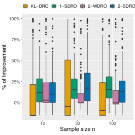
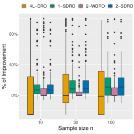
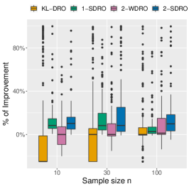
Figure 2: Out-of-sample performance for the newsvendor model with parameters $s\in\{0.25,0.5,0.75,1,2,4\}$ and fixed sample size $n=20$. The $y$-axis corresponds to the coefficent of prescriptiveness defined in (15). For figures from left to right, we specify the data distribution as exponential distribution, gamma distribution, and equiprobable mixture of two truncated normal distributions, respectively.

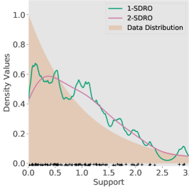
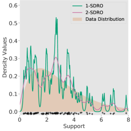
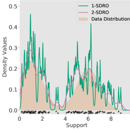
Figure 3: Plots for the density of worst-case distributions generated by the $1$-SDRO or $2$-SDRO model. The black dots in the bottom of figures indicate the sample points from the training dataset of sample size $n=100$. For figures from left to right, we specify the data distribution as exponential distribution, gamma distribution, and equiprobable mixture of two truncated normal distributions, respectively.

We report the box-plots of the coefficients of prescriptiveness in Fig. 2 using $200$ independent trials. We find that either $1$-SDRO or $2$-SDRO model achieve the best out-of-sample performance over all sample sizes and data distributions listed, as it consistently scores higher than other benchmarks in the box plots. In contrast, the KL-DRO model does not achieve satisfactory performance, and sometimes even underperforms the SAA model. While the $2$-WDRO model demonstrates some improvement over the SAA model, the $2$-SDRO model shows more clear improvement. Additionally, we plot the density of worst-case distributions for $1$-SDRO or $2$-SDRO model in Fig. 3. When specifying the data distribution as exponential, gamma, or Gaussian mixture, the corresponding worst-case distributions capture the shape of the ground truth distribution reasonably well, which partly explains why the Sinkhorn DRO model achieves superior performance when the data distribution is absolutely continuous.

5.2 Mean-risk Portfolio Optimization

Consider the following distributionally robust mean-risk portfolio optimization problem

$$\min_{\theta}\max_{\mathbb{P}\in\mathbb{B}_{\rho,\epsilon}(\widehat{\mathbb{P}})} \quad\mathbb{E}_{z\sim\mathbb{P}}[-\theta^{\mathrm{T}}z]+\varrho\cdot\text{$\mathbb{P}$-CVaR}_{\alpha}(-\theta^{\mathrm{T}}z)$$

s.t. $$\quad\theta\in\Theta=\{\theta\in\mathbb{R}^{d}_{+}:\,\theta^{\mathrm{T}}1=1\},$$

where the random vector $z\in\mathbb{R}^{d}$ stands for the returns of assets; the decision variable $\theta\in\Theta$ represents the portfolio strategy that invests a certain percentage $\theta_{i}$ of the available capital in the $i$-th asset; and the term $\text{$\mathbb{P}$-CVaR}_{\alpha}(-\theta^{\mathrm{T}}z)$ quantifies conditional value-at-risk [98], i.e., the average of the $\alpha\times 100\%$ worst portfolio losses under the distribution $\mathbb{P}$. We follow a similar setup as in [78]. Specifically, we set $\alpha=0.2,\varrho=10$. The underlying true random return can be decomposed into a systematic risk factor $\psi\in\mathbb{R}$ and idiosyncratic risk factors $\epsilon\in\mathbb{R}^{d}$:

$$z_{i}=\psi+\epsilon_{i},\quad i=1,2,\ldots,d,$$

where $\psi\sim\mathcal{N}(0,0.02)$ and $\epsilon_{i}\sim\mathcal{N}(i\times 0.03,i\times 0.025)$. When solving the Sinkhorn DRO formulation, we take the Bregman divergence $D_{\omega}$ as the KL-divergence when performing BSMD algorithm in Algorithm 1, allowing for efficient implementation [82]. We quantify the performance of a given solution using the same criterion defined in Section 5.1 and generate box plots using $200$ independent trials. Fig. 4a) reports the scenario where the data dimension $d=30$ is fixed and sample size $n\in\{30,50,100,150,200,400\}$, and Fig. 4b) reports the scenario where the sample size $n=100$ is fixed and the number of assets $d\in\{5,10,20,40,80,100\}$. We find that the KL-DRO model does not have competitive performance compared to other DRO models, especially as the data dimension $d$ increases. This is because the ambiguity set of KL-DRO model only takes into account those distributions sharing the same support as the nominal distribution, which seems to be restrictive, especially for high-dimensional settings. Moreover, while $1$-WDRO or $2$-WDRO model has better out-of-sample performance than the SAA model, the corresponding $1$-SDRO or $2$-SDRO model has clearer improvements, as it consistently scores higher in the box plots.

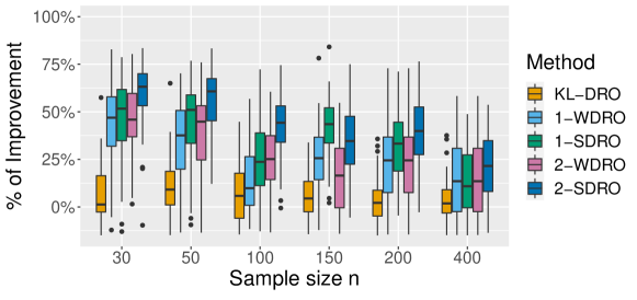
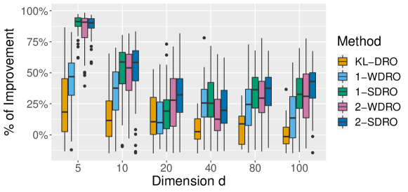
Figure 4: Out-of-sample performance for the portfolio optimization problem. Upper: fixing data dimension $d=30$ and varying sample size $n\in\{30,50,100,150,200,400\}$. Bottom: fixing sample size $n=100$ and varying data dimension $d\in\{5,10,20,40,80,100\}$.

5.3 Adversarial Multi-class Logistic Regression

The adversarial attack is an emerging topic in artificial intelligence: small perturbations to the data-generating distribution can cause well-trained machine learning models to produce unexpectedly inaccurate predictions [55]. For real applications involving high-stake environments, such as self-driving and automated detection of tumors, it is critical to deploy models which are robust to potential adversarial attacks. Many approaches for adversarial attack and defense have been proposed in literature [86, 87, 88, 99, 109, 58, 76, 116]. Among those approaches, DRO is a promising training procedure that guarantees certifiable adversarial robustness [109]. In this subsection, we consider an adversarial training model for multi-class logistic regression. Given a feature vector $x\in\mathbb{R}^{d}$ and its label $y\in[C]$, we denote ${\bm{y}}\in\{0,1\}^{C}$ as the corresponding one-hot label vector, and define the following negative likelihood loss:

$$h_{B}(x,{\bm{y}})=-{\bm{y}}^{\mathrm{T}}B^{\mathrm{T}}x+\log\big{(}1^{\mathrm{T}}e^{B^{\mathrm{T}}x}\big{)},$$

where $B:=[w_{1},\ldots,w_{K}]$ stands for the linear classifier. Let $\widehat{\mathbb{P}}$ be the empirical distribution from training samples. Since the testing samples may have slightly different data distributions than the training samples, the DRO model aims to solve the following optimization problem to mitigate the impact of adversarial attacks:

$$\min_{B}~{}\max_{\mathbb{P}\in\mathbb{B}_{\rho,\epsilon}(\widehat{\mathbb{P}})} \quad\mathbb{E}_{(x,{\bm{y}})\sim\mathbb{P}}\big{[}h_{B}(x,{\bm{y}})\big{]}.$$

It is assumed that only the feature vector $x$ has uncertainty but not the label ${\bm{y}}$.

We conduct experiments on four large-scale datasets: CIFAR10 [65], CIFAR100 [65], STL10 [30], and tinyImageNet [115]. We pre-process these datasets using the ResNet-18 network [57] pre-trained on the ImageNet dataset to extract linear features. Since this network has learned a rich set of hierarchical features from the large and diverse ImageNet dataset, it typically extracts useful features for other image datasets. We then add various perturbations to the testing datasets, such as $\ell_{1}$-norm and $\ell_{2}$-norm adversarial projected gradient method attacks [76], white Laplace noise, and white Gaussian noise, to evaluate the performance of the DRO models. See the detailed procedure for generating adversarial perturbations and statistics on pre-processed datasets in Appendix 7.3. We use the mis-classification rate on testing dataset to quantify the performance for the obtained classifers.

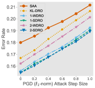
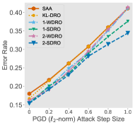
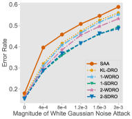
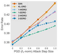
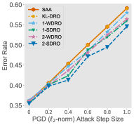
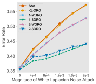
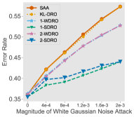
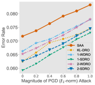
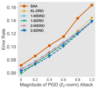
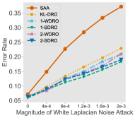
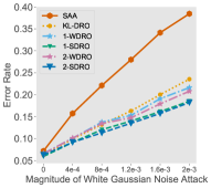
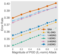
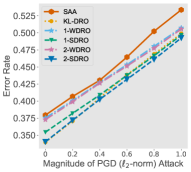
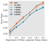
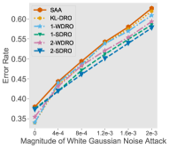
Figure 5: Results of adversarial training on various image datasets with different types of adversarial attack. From left to right, the figures correspond to (a) $\ell_{1}$-norm PGD attack; (b) $\ell_{2}$-norm PGD attack; (c) white Laplacian noise attack; and (d) white Gaussian noise attack. From top to bottom, the figures correspond to (a) CIFAR10 dataset; (b) CIFAR100 dataset; (c) STL10 dataset; and (d) tinyImageNet dataset.

For baseline DRO models, we solve their penalized formulations and tune the Lagrangian multiplier to obtain the best performance. However, solving the penalized $2$-WDRO model is tractable only when the multiplier is sufficiently large [109], and all its maximization subproblems involve concave objective functions, which may not be the case for practical experiments. Additionally, the penalized $1$-WDRO model is a convex-non-concave minimax game in high dimensions, making it intractable to solve into global optimality, with the exception that when the number of classes $C=2$, it reduces to the tractable distributionally robust logistic regression model [104]. To approximately solve these WDRO formulations, we try gradient descent ascent heuristics, which are inspired from [109, Algorithm 1] (see Algorithm 4 in Appendix 7.3), but they are computationally inefficient and do not yield satisfactory classifiers. To make a fair comparison, we solve the soft formulation of KL-DRO, $1$-SDRO, or $2$-SDRO in this subsection and tune the hyper-parameter $\lambda$.

Figure 5 presents the classification results for different types of adversarial attacks with varying levels of perturbations on the datasets. We observe that as the level of perturbations on the testing samples increases, all methods tend to perform worse. However, both the $1$-SDRO and $2$-SDRO models show a slower trend of increasing error rates than other benchmarks across all types of adversarial attacks and all datasets. This suggests that SDRO models can be a suitable choice for adversarial robust training.

6 Concluding Remarks

In this paper, we investigated a new distributionally robust optimization framework based on the Sinkhorn distance. By developing a strong dual reformulation and a biased stochastic mirror descent algorithm, we have shown that the resulting problem is tractable under mild assumptions, which significantly spans the tractability of Wasserstein DRO. Analysis of the worst-case distribution indicates that Sinkhorn DRO hedges a more reasonable set of adverse scenarios and is thus less conservative than Wasserstein DRO. Extensive numerical experiments demonstrated that Sinkhorn DRO is a promising candidate for modeling distributional ambiguities in decision-making under uncertainty.

In the meantime, several topics worth investigating are left for future work. For example, one important research question is the statistical performance guarantees under suitable choices of hyper-parameters. Exploring and discovering the benefits of Sinkhorn DRO in other applications may also be of future interest.

Supplementary for “Sinkhorn Distributionally Robust Optimization”

7 Detailed Experiment Setup

The experiments were conducted on a MacBook Pro laptop with 32GB of memory running Python 3.7. Unless stated otherwise, we solved the SAA, Wasserstein DRO, and KL-divergence DRO baseline models exactly using the interior point method-based solver Mosek [4]. Optimization hyperparameters, such as step size, maximum iterations, and number of levels, were tuned to minimize training error after 10 outer iterations. We use RT-MLMC gradient estimator to solve the Sinkhorn DRO model. We employed the warm starting strategy during the iterative procedure: we set the initial guess of parameter $\theta$ at the beginning of outer iteration as the one obtained from the SAA approach. At other outer iterations, the initial guess of parameter $\theta$ is set to be the final obtained solution $\theta$ at the last outer iteration. The following subsections outline some special reformulations, optimization algorithms used to solve the baseline models together with the running time of all approaches.

7.1 Setup for Newsvendor Problem and Running Time

To solve the $2$-Wasserstein DRO model with radius $\rho$, we approximate the support of worst-case distribution using discrete grid points. Denote by $\mathcal{D}_{n}=\{x_{1},\ldots,x_{n}\}$ the set of observed $n$ samples and $\mathcal{G}_{200-n}$ the set of $200-n$ points evenly supported on the interval $[0,10]$. Then the support of worst-case distribution is restricted to $\mathcal{D}_{n}\cup\mathcal{G}_{200-n}:=\{\hat{z}_{1},\ldots,\hat{z}_{200}\}$. The corresponding $2$-Wasserstein DRO problem has the following linear programming reformulation:

$$\min_{\theta,\lambda,s} \quad\lambda\rho+\frac{1}{n}\sum_{i=1}^{n}s_{i}$$

s.t. $$\quad k\theta-u\min(\theta,\hat{z}_{j})-\lambda(x_{i}-\hat{z}_{j})^{2}\leq s_{i},\quad\forall i\in[n],\forall j\in[200].$$

The computational time for the newsvendor problem in Section 5.1 is reported in Table 3. We observe that the training time of $2$-Wasserstein DRO model increases quickly as the sample size increases, while the training time of other DRO models increases mildly in the training sample size.

Table 3: Average computational time (in seconds) per problem instance for the newsvendor problem.

Model	Exponential			Gamma			Gaussian Mixture
	$n=10$	$n=30$	$n=100$	$n=10$	$n=30$	$n=100$	$n=10$	$n=30$	$n=100$
SAA	0.017	0.017	0.018	0.019	0.019	0.019	0.023	0.024	0.024
KL-DRO	0.027	0.029	0.040	0.027	0.028	0.039	0.027	0.028	0.038
1-SDRO	0.110	0.124	0.161	0.105	0.119	0.162	0.105	0.119	0.157
2-WDRO	0.123	0.358	1.307	0.128	0.354	1.337	0.134	0.402	1.428
2-SDRO	0.061	0.069	0.106	0.100	0.121	0.161	0.095	0.115	0.154

7.2 Setup for Mean-risk Portfolio Optimization and Running Time

From [78, Eq. (27)] we can see that the $1$-Wasserstein DRO formulation with radius $\rho$ for the portfolio optimization problem becomes

$$\min_{\theta,\tau,\lambda,s} \quad\lambda\rho+\frac{1}{n}\sum_{i=1}^{n}s_{i}$$

s.t. $$\quad\theta\in\Theta,\quad b_{j}\tau+a_{j}\langle\theta,\hat{z}_{i}\rangle\leq s_{i},i\in[n],j\in[H],$$

$$\quad\|a_{j}\theta\|_{2}\leq\lambda,j\in[H].$$

Also, we argue that the $2$-Wasserstein DRO formulation with radius $\rho$ for the portfolio optimization problem has a finite convex reformulation:

$$\inf_{\theta\in\Theta,\tau}~{}\sup_{\mathbb{P}:~{}W_{2}(\mathbb{P},\widehat{\mathbb{P}}_{n})\leq\rho}\mathbb{E}_{\mathbb{P}}\big{[}\max_{j\in[H]}a_{j}\langle\theta,z\rangle+b_{j}\tau\big{]}$$

$$= \inf_{\theta\in\Theta,\tau,\lambda\geq 0}~{}\left\{\lambda\rho^{2}+\frac{1}{n}\sum_{i=1}^{n}\sup_{s_{i}}~{}\left\{\max_{j\in[H]}a_{j}\langle\theta,s_{i}\rangle+b_{j}\tau-\lambda\|s_{i}-\hat{z}_{i}\|_{2}^{2}\right\}\right\}.$$

In particular, the inner subproblem has the following reformulation:

$$\sup_{s_{i}}~{}\left\{\max_{j\in[H]}a_{j}\langle\theta,s_{i}\rangle+b_{j}\tau-\lambda\|s_{i}-\hat{z}_{i}\|_{2}^{2}\right\}$$

$$= \max_{j\in[H]}~{}b_{j}\tau+\sup_{s_{i}}\left\{a_{j}\langle\theta,s_{i}\rangle-\lambda\|s_{i}-\hat{z}_{i}\|_{2}^{2}\right\}$$

$$= \max_{j\in[H]}~{}b_{j}\tau+\frac{a_{j}^{2}}{4\lambda}\|\theta\|^{2}_{2}+a_{j}\langle\theta,\hat{z}_{i}\rangle.$$

Hence, the $2$-Wasserstein DRO can be reformulated as

$$\min_{\theta,\tau,\lambda,s} \quad\lambda\rho^{2}+\frac{1}{n}\sum_{i=1}^{n}s_{i}$$

s.t. $$\quad\theta\in\Theta,\quad b_{j}\tau+a_{j}\langle\theta,\hat{z}_{i}\rangle+\frac{a_{j}^{2}}{4\lambda}\|\theta\|_{2}^{2}\leq s_{i},\quad i\in[n],j\in[H].$$

The computational time for the portfolio optimization problem in Section 5.2 is reported in Table 4. We observe that when the data dimension is fixed and the sample size varies from $30$ to $400$, the computational time for all approaches does not differ too much. When the data dimension increases and the sample size is fixed, the computational time for $1$-SDRO or $2$-SDRO model increases linearly while other DRO models increase mildly. One possible explanation is that in this example, other DRO models have tractable finite-dimensional conic programming formulations so that off-the-shelf software can solve them efficiently. In contrast, Sinkhorn DRO models do not have special reformulation, but they can still be solved in a reasonable amount of time.

Table 4: Average computational time (in seconds) per problem instance for portfolio optimization problem.

$(n,d)$ Values	SAA	KL-DRO	1-WDRO	1-SDRO	2-WDRO	2-SDRO
$(30,30)$	0.013	0.038	0.018	0.125	0.015	0.090
$(50,30)$	0.014	0.042	0.020	0.163	0.016	0.110
$(100,30)$	0.017	0.065	0.024	0.167	0.021	0.144
$(150,30)$	0.019	0.084	0.029	0.158	0.027	0.152
$(200,30)$	0.023	0.115	0.035	0.151	0.032	0.150
$(400,30)$	0.045	0.136	0.061	0.167	0.056	0.142
$(100,5)$	0.014	0.043	0.017	0.082	0.015	0.111
$(100,10)$	0.014	0.045	0.018	0.109	0.015	0.128
$(100,20)$	0.014	0.048	0.021	0.138	0.017	0.187
$(100,40)$	0.017	0.068	0.027	0.179	0.022	0.269
$(100,80)$	0.021	0.103	0.052	0.357	0.044	0.462
$(100,100)$	0.023	0.116	0.070	0.387	0.059	0.478

7.3 Setup for Adversarial Multi-class Logistic Regression and Running Time

The procedure for generating various adversarial perturbations is reported in the following:

1. For a given classifer $B$ and data sample $(x,{\bm{y}})$, the $\ell_{p}$-norm ($p\in\{1,2\}$) adversarial attack based on projected gradient method [76] iterates as follows: $x_{0}\leftarrow x$ and

   $$\left\{\begin{aligned} \Delta x^{k+1}&\leftarrow\argmax_{\|\eta\|_{p}\leq\xi}~{}\Big{\{}\nabla_{x}h_{B}(x^{k},{\bm{y}})^{\mathrm{T}}\eta\Big{\}},\\ x^{k+1}&\leftarrow\text{Proj}_{\{x^{\prime}:~{}\|x-x^{\prime}\|_{p}\leq\xi\}}~{}\Big{\{}x^{k}+\frac{\alpha}{\sqrt{k+1}}\Delta x^{k+1}\Big{\}}.\end{aligned}\right.$$

   We perform the gradient update above for $15$ steps. Also, we specify the initial learning rate $\alpha=1$ and vary the radius of attack $\xi\in\{0,0.2,0.4,0.6,0.8,1\}$.

2. For a given feature vector $x$, the perturbed feature using white Laplacian noise becomes $x+\xi\|x\|_{2}\cdot\zeta$, where the random vector $\zeta$ follows the isotropic Laplace distribution with zero mean and unit variance, and we vary the ratio $\xi\in\{0,4\cdot 10^{-4},8\cdot 10^{-4},1.2\cdot 10^{-3},1.6\cdot 10^{-3},2\cdot 10^{-3}\}.$ Similarly, the perturbed feature using white Gaussian noise becomes $x+\xi\|x\|_{2}\cdot\zeta$, with $\zeta$ being the isotropic Gaussian distribution with zero mean and unit variance. Our experiment setup that adds white noise is inspired from [23, Section 4].

In this example, we use stochastic gradient methods to solve the SAA formulation and all penalized DRO formulations. Inspired from classical adversarial training approaches that usually require fine-tuning of hyper-parameters via grid search [25], we fine-tune the hyper-parameters (i.e., Lagrangian multiplier $\lambda$ or regularization value $\epsilon$) of DRO formulations from the following grid of values and report the optimal performance:

• KL-DRO/$1$-WDRO/$2$-WDRO: $\lambda\in\{0.05,0.1,0.5,1,3,5,10,15,20,25,30,100\}$.

• $1$-SDRO/$2$-SDRO: $\lambda\in\{1,5,10\}$ and $\epsilon\in\{0.1,0.5,1\}$.

We terminate the training of SAA or DRO models when the number of epoches, i.e., the number of times for processes each training sample, exceeds $30$. In is worth mentioning that the Wasserstein DRO model with a fixed Lagrangian multiplier $\lambda$ using samples $\{x_{i},{\bm{y}}_{i}\}_{i=1}^{n}$ can be reformulated as

$$\min_{B}~{}\frac{1}{n}\sum_{i=1}^{n}~{}\left[\max_{x\in\mathbb{R}^{d}}~{}\Big{\{}h_{B}(x,{\bm{y}}_{i})-\lambda c(x_{i},x)\Big{\}}\right].$$ (16)

To approximately solve such a convex-non-concave problem, we implement a gradient descent ascent heuristic outlined in Algorithm 4. We report basic statistics of classification datasets in this example in Table 5. Besides, the computational time is reported in Table 6. The results indicate that Sinkhorn DRO models have shorter computational time than Wasserstein DRO models in general.

Table 5: Basic statistics of adversarial multi-class logistic regression datasets.

	CIFAR10	CIFAR100	STL10	tinyImageNet
$\begin{array}[]{c}\mbox{Image Size}\\ \mbox{(before pre-processing)}\end{array}$	3072	3072	27648	12288
$\begin{array}[]{c}\mbox{Feature Dimension}\\ \mbox{(after pre-processing)}\end{array}$	512	512	512	512
$\#$ of classes	10	100	10	200
Training Size	50000	50000	5000	90000
Testing Size	10000	10000	8000	10000

Table 6: Average computational time (in seconds) per problem instance for adversarial multi-class logistic regression problem

Dataset	SAA	KL-DRO	1-WDRO	1-SDRO	2-WDRO	2-SDRO
CIFAR10	10.55	12.11	55.10	59.52	53.04	47.26
CIFAR100	15.64	16.01	125.31	114.99	128.20	106.62
STL10	1.37	1.59	7.36	7.34	7.96	6.99
tinyImageNet	45.54	44.50	325.25	227.91	347.16	197.55

Algorithm 4 Heuristic Gradient Descent Ascent algorithm (inspired from [109, Algorithm 1]) for solving (16). We use default values $\alpha=\texttt{1e-2},m=100,n_{\text{critic}}=15$.

0:   Learning rate $\alpha$, batch size $m$, number of inner iterations $n_{\text{critic}}$, number of outer iterations $T_{\text{out}}$, initial guess $B$.

1:  for $t_{\text{out}}=0,1,\ldots,T_{\text{out}}-1$ do

2:     Sample a subset of indices $\{n_{i}\}_{i=1}^{m}$ from $[n]$.

3:     Initialize $\hat{x}_{n_{i}}\leftarrow x_{n_{i}},i\in[m]$.

4:     for $t=0,1,\ldots,n_{\text{critic}}-1$ do

5:         Compute $g_{n_{i}}\leftarrow\nabla_{z_{n_{i}}}\big{[}h_{B}(\hat{x}_{n_{i}},{\bm{y}}_{n_{i}})-\lambda c(\hat{x}_{n_{i}},x_{n_{i}})\big{]}$ for $i\in[m]$.

6:         Update $\hat{x}_{n_{i}}\leftarrow\hat{x}_{n_{i}}+\alpha\text{Adam}(\hat{x}_{n_{i}},g_{n_{i}})$ for $i\in[m]$.

7:     end for

8:      Compute $g_{B}\leftarrow\nabla_{B}\Big{[}\frac{1}{m}\sum_{i=1}^{m}h_{B}(\hat{x}_{n_{i}})\Big{]}$.

9:      Update $B\leftarrow B-\alpha\text{Adam}(B,g_{B})$.

10:  end forOutput $B$.

8 Additional Validation Experiments

8.1 Comparison of Optimization Algorithms: Distributionally Robust Linear Regression

To examine the performance of different gradient estimators, we study the problem of distributionally robust linear regression (see the setup in Example 3.7). We take the nominal distribution $\widehat{\mathbb{P}}$ as the empirical one based on samples $\{(a_{i},b_{i})\}_{i=1}^{n}$. As a consequence, the inner objective function in (10) has the closed form expression:

$$F(\theta)=\frac{1}{n}\sum_{i=1}^{n}(a_{i}^{\mathrm{T}}\theta-b_{i})^{2}+\frac{\frac{1}{n}\sum_{i=1}^{n}(a_{i}^{\mathrm{T}}\theta-b_{i})^{2}}{\frac{1}{2}\lambda\|\theta\|_{2}^{-2}-1}-\frac{\lambda\epsilon}{2}\log\det\left(I-\frac{\theta\theta^{\mathrm{T}}}{\frac{1}{2}\lambda}\right),\quad\text{if }\|\theta\|_{2}^{2}<\frac{\lambda}{2},$$

and otherwise $F(\theta)=\infty$. We take the constraint set $\Theta=\{\theta:~{}\|\theta\|_{2}^{2}\leq 0.999\cdot\frac{\lambda}{2}\}$. Similar to the setup in [69, Section 5.1], we examine the performance using three LIBSVM regression real world datasets [70]: housing, mg, and mpg.

The quality of proposed gradient estimators is examined in a single BSMD step with specified hyper-parameters $(\lambda,\epsilon)=(10^{3},10^{-1})$. For baseline comparison, we also study the performance of the standard MLMC scheme. It has been shown in [60] that this gradient estimator achieves the same sample complexity rate as RT-MLMC estimator for convex smooth CSO problem. However, this estimator will lead to sub-optimal complexity rate compared with RT-MLMC when the inner objective function is no longer smooth. We verify its performance in a toy experiment with a convex nonsmooth loss function in the next subsection.
MLMC Estimator: Fix some number $N>0$. For $\ell=0,1,\ldots,L$, get $n_{\ell}:=\lceil 2^{-\ell}N\rceil$ random variables $\{A^{\ell}(\theta,\zeta^{\ell}_{i})\}_{i=1}^{n_{\ell}}$, where $\{\zeta_{i}^{\ell}\}_{i}$ are i.i.d. copies of $\zeta^{\ell}$. Construct

$$\widehat{F}^{\text{MLMC}}(\theta)=\sum_{\ell=0}^{L}\frac{1}{n_{\ell}}\sum_{i=1}^{n_{\ell}}A^{\ell}(\theta,\zeta^{\ell}_{i}).$$ (17)

Besides, we also compare two unbiased gradient estimators in literature [60]. However, the variance of them are unbounded, so that there is no convergence analysis for those two methods.
RU-MLMC Estimator: at point $\theta$, we sample a random level $\iota$, following a distribution $\mathbb{P}(\iota=\ell)=q_{\ell},\ell=0,1,\ldots,\infty,$ where the probability mass value $q_{\ell}\propto 2^{-\ell}$. Then construct

$$v^{\text{RU-MLMC}}(\theta):=\frac{1}{q_{\iota}}G^{\iota}(\theta,\zeta^{\iota}).$$ (18)

RR-MLMC Estimator: at point $\theta$, we sample a random level $L$, following a distribution $\mathbb{P}(\iota=\ell)=q_{\ell},\ell=0,1,\ldots,\infty,$ where the probability mass value $q_{\ell}\propto 2^{-\ell}$. Then construct

$$v^{\text{RR-MLMC}}(\theta):=\sum_{\ell=0}^{L}p_{\ell}G^{\ell}(x,\zeta^{\ell}),$$ (19)

where $p_{\ell}:=\frac{1}{1-\sum_{\ell^{\prime}=0}^{\ell-1}q_{\ell^{\prime}}}$ and $\sum_{\ell^{\prime}=0}^{-1}q_{\ell^{\prime}}=0$.

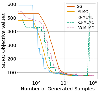
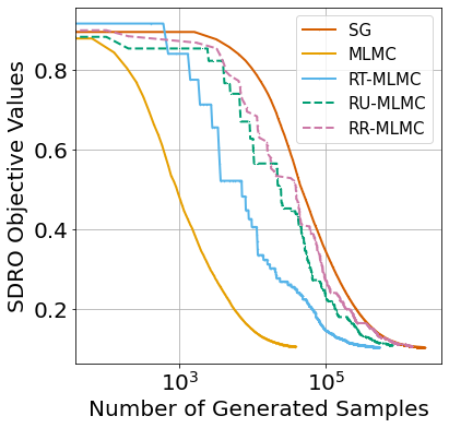
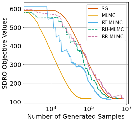
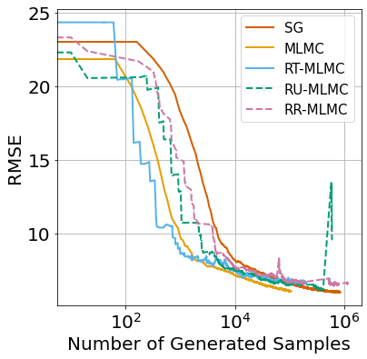
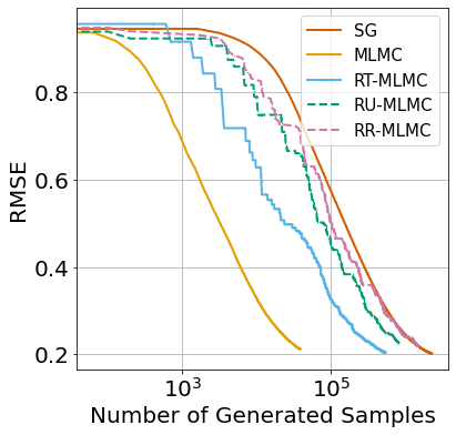
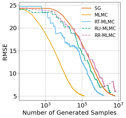
Figure 6: Comparison results of SG, MLMC, RT-MLMC, RU-MLMC, and RR-MLMC on robust linear regression problem. From left to right, the figures correspond to three different regression datasets: (a) housing; (b) mg; and (c) mpg. From top to bottom, the figures correspond to plots of (a) Sinkhorn DRO objective values; and (b) RMSE of obtained solutions.

For a given solution $\theta$, we quantify its performance using the corresponding Sinkhorn DRO objective value. Besides, we report its root-mean-square error (RMSE) on training data. Thus, the smaller those two performance criteria are, the smaller the solution’s optimization performance has. Figure 6 shows the performance of various gradient estimators in terms of the number of generated samples based on these criteria. The results demonstrate that the SG scheme does not perform competitively, as expected from our theoretical analysis that shows SG has the worst complexity order. In contrast, using other four types of MLMC methods, we can obtain optimal solutions with small sample complexity. While the RU-MLMC and RR-MLMC schemes exhibit competitive performance, the optimization procedure shows some oscillations. One possible explanation is that the variance values of those gradient estimators are unbounded, making these two approaches unstable.

8.2 Comparison of Optimization Algorithms: Distributionally Robust Portfolio Optimization

In this subsection, we validate the competitive performance of RT-MLMC gradient estimator on the case where the loss is convex and nonsmooth, and we try to solve the $2$-SDRO formulation. We consider the portfolio optimization problem, and specify different choices of the problem parameters (sample size $n$ and data dimension $d$) as $(50,50),(100,100),(400,400)$. We quantify the performance of obtained solution using the Sinkhorn DRO objective value. Since in this problem setup no analytical expression of the objective value is available, we estimate the objective value using (14) with hyper-parameters $L=8$ and $n^{\mathrm{o}}_{L}=10^{3}$. Figure 7 shows the performance in terms of the number of generated samples based on this criterion. The results demonstrate that even for nonsmooth loss function, those listed MLMC-based gradient estimators have better performance than the SG scheme. Besides, the proposed RT-MLMC and standard MLMC schemes have comparable performance, and in some cases MLMC scheme even has better performance. It is an open question that whether the MLMC scheme will have the same order of sample complexity as the RT-MLMC scheme for convex nonsmooth optimization, which can be a topic for future study.

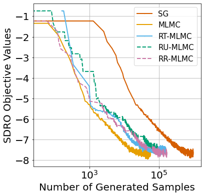
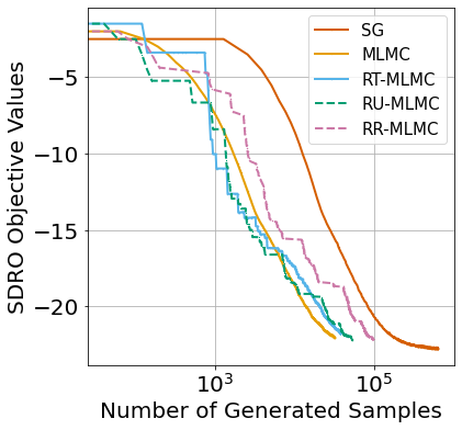
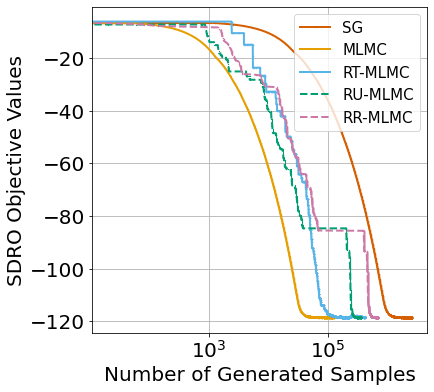
Figure 7: Comparison results of SG, MLMC, RT-MLMC, RU-MLMC, and RR-MLMC on robust portfolio optimization problem. From left to right, the figures correspond to three different specifications of $(n,d)\in\{(50,50),(100,100),(400,400)\}$.

8.3 Sensitivity of Regularization Parameters

In this subsection, we validate the impact of regularization parameter $\epsilon$ on the performance of the Sinkhorn DRO model in two numerical examples: newsvendor and portfolio optimization problem. We examine the performance of $1$-SDRO or $2$-SDRO models for different regularization parameters chosen from the candidate set $\mathcal{A}$:

$$\mathcal{A}=\left\{\begin{aligned} \{10^{-3},5\cdot 10^{-3},10^{-2},5\cdot 10^{-2},10^{-1},5\cdot 10^{-1},10^{0}\},&\quad\text{for newsvendor problem},\\ \{5\cdot 10^{-2},10^{-1},5\cdot 10^{-1},10^{0},3\cdot 10^{0},5\cdot 10^{0},10^{1}\},&\quad\text{for portfolio optimization}.\end{aligned}\right.$$

For each fixed regularization parameter $\epsilon$, we tune the corresponding Sinkhorn DRO radius $\overline{\rho}$ by cross validation. We quantify the performance of a given solution $\theta$ obtained from DRO models using the performance gap metric $\frac{J(\theta)-J^{*}}{1+|J^{*}|},$ where notations $J^{*}$ and $J(\theta)$ are defined at the beginning of Section 5. Hence, the smaller the metric is, the better the given decision has.

Fig. 8 shows box plots on the performance of Sinkhorn DRO models across different choices of regularization values with different data distributions on the newsvendor problem. We can see as the regularization value increases, the performance of Sinkhorn DRO models generally improves first and then degrades.

Fig. 9 shows performance on the portfolio optimization problem with different choices of problem parameters $(n,d)$, where $n$ denotes the sample size and $d$ denotes the data dimension. Compared with the newsvendor problem, we find a more clear trend that the model performance improves and then degrades as the regularization value increases. In this special example, we also find $2$-SDRO model has more stable and satisfactory performance compared with $1$-SDRO model.

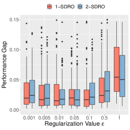
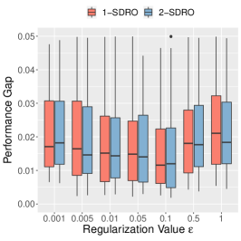
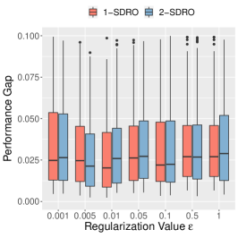
Figure 8: Performance of Sinkhorn DRO models for newsvendor problem versus different choices of regularization values $\epsilon$. For figures from left to right, we specify the data distribution as exponential distribution, gamma distribution, and equiprobable mixture of two truncated normal distributions, respectively.

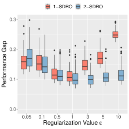
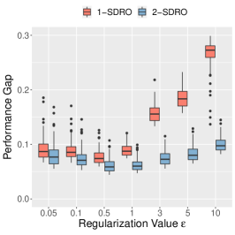
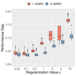
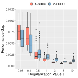
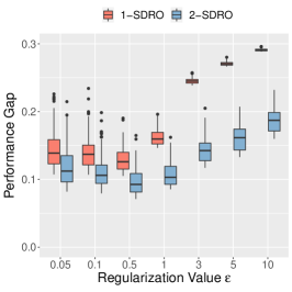
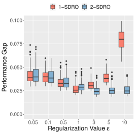
Figure 9: Performance of Sinkhorn DRO models for portfolio problem versus different choices of regularization values $\epsilon$. For those fix figures from left to right, from top to bottom, we specify the problem parameters (sample size $n$ and data dimension $d$) as $(30,30),(100,30),(400,30),(100,5),(100,20),(100,100)$, respectively.

9 Sufficient Condition for Condition 1

Proposition 9.1

Condition 1 holds if there exists $p\geq 1$ so that the following conditions are satisfied:

1. For any $x,y,z\in\mathcal{Z}$, $c(x,y)\geq 0$, and $(c(x,y))^{1/p}\leq(c(x,z))^{1/p}+(c(z,y))^{1/p}.$

2. The nominal distribution $\widehat{\mathbb{P}}$ has a finite mean, denoted as $\overline{x}$. Moreover, $\nu\{z:~{}0\leq c(\overline{x},z)<\infty\}=1$ and $\Pr{}_{x\sim\widehat{\mathbb{P}}}\{c(x,\overline{x})<\infty\}=1.$

3. Assumption 3.1(III) holds, and there exists $\lambda>0$ such that

   $$\mathbb{E}_{z\sim\nu}\left[e^{f(z)/(\lambda\epsilon)}e^{-2^{1-p}c(\overline{x},z)/\epsilon}\right]<\infty.$$

We make some remarks for the sufficient conditions listed above. The first condition can be satisfied by taking the transport cost as the $p$-th power of the metric defined on $\mathcal{Z}$ for any $p\geq 1$. The second condition requires the nominal distribution $\widehat{\mathbb{P}}$ is finite almost surely, e.g., it can be a subguassian distribution with respect to the transport cost $c$. We first present an useful technical lemma before showing the proof of Proposition 9.1.

Lemma 9.2

Under the first condition of Proposition 9.1, for any $x\in\mathcal{Z}$, it holds that

$$\mathbb{E}_{z\sim\nu}\left[\int e^{-c(x,z)/\epsilon}\right]\geq e^{-2^{p-1}c(x,\overline{x})/\epsilon}\mathbb{E}_{z\sim\nu}\left[e^{-2^{p-1}c(\overline{x},z)/\epsilon}\right].$$

Proof 9.3

Proof of Lemma 9.2. Based on the inequality $(a+b)^{p}\leq 2^{p-1}(a^{p}+b^{p})$, we can see that

$$c(x,z)\leq(c(y,z)^{1/p}+c(z,y)^{1/p})^{p}\leq 2^{p-1}(c(y,z)+c(z,y)),\quad\forall x,y,z\in\mathcal{Z}.$$

Since $c(x,z)\leq 2^{p-1}(c(\overline{x},z)+c(x,\overline{x}))$, we can see that

$$\mathbb{E}_{z\sim\nu}\left[\int e^{-c(x,z)/\epsilon}\right] \geq\exp\left(-2^{p-1}c(x,\overline{x})/\epsilon\right)\mathbb{E}_{z\sim\nu}\left[e^{-2^{p-1}c(\overline{x},z)/\epsilon}\right].$$

The proof is completed.  $\square$

Proof 9.4

Proof of Proposition 9.1. One can see that for any $x\in\mathrm{supp}\,\widehat{\mathbb{P}}$, it holds that

$$\mathbb{E}_{z\sim\mathbb{Q}_{x,\epsilon}}\left[e^{f(z)/(\lambda\epsilon)}\right]$$

$$= \mathbb{E}_{z\sim\nu}\left[e^{f(z)/(\lambda\epsilon)}\frac{e^{-c(x,z)/\epsilon}}{\mathbb{E}_{u\sim\nu}\left[e^{-c(x,u)/\epsilon}\right]}\right]$$

$$\leq \mathbb{E}_{z\sim\nu}\left[e^{f(z)/(\lambda\epsilon)}\frac{e^{-c(x,z)/\epsilon}}{\mathbb{E}_{u\sim\nu}\left[e^{-2^{p-1}c(\overline{x},u)/\epsilon}\right]}\right]$$

$$\leq \mathbb{E}_{z\sim\nu}\left[e^{f(z)/(\lambda\epsilon)}\frac{e^{-2^{1-p}c(\overline{x},z)/\epsilon}e^{c(x,\overline{x})/\epsilon}}{\mathbb{E}_{u\sim\nu}\left[e^{-2^{p-1}c(\overline{x},u)/\epsilon}\right]}\right]$$

$$= \frac{e^{c(x,\overline{x})(1+2^{p-1})/\epsilon}}{\mathbb{E}_{u\sim\nu}\left[e^{-2^{p-1}c(\overline{x},u)/\epsilon}\right]}\mathbb{E}_{z\sim\nu}\left[e^{f(z)/(\lambda\epsilon)}e^{-2^{1-p}c(\overline{x},z)/\epsilon}\right],$$

where the first inequality is based on the lower bound in Lemma 9.2, the second inequality is based on the triangular inequality $c(x,z)\geq 2^{1-p}c(\overline{x},z)-c(x,\overline{x})$. Note that almost surely for all $x\in\mathrm{supp}\,\widehat{\mathbb{P}}$, $c(x,\overline{x})<\infty$. Moreover,

$$0<\mathbb{E}_{z\sim\nu}\left[e^{-2^{p-1}c(\overline{x},z)/\epsilon}\right]\leq\mathbb{E}_{z\sim\nu}\left[e^{-c(\overline{x},z)/\epsilon}\right]<\infty,$$

where the lower bound is because $c(\overline{x},z)<\infty$ almost surely for all $z$, the upper bound is because $c(\overline{x},z)\geq 0$ almost surely for all $z$. Based on these observations, we have that

$$\mathbb{E}_{z\sim\mathbb{Q}_{x,\epsilon}}\left[e^{f(z)/(\lambda\epsilon)}\right]\leq\frac{e^{c(x,\overline{x})(1+2^{p-1})/\epsilon}}{\mathbb{E}_{z\sim\nu}\left[e^{-2^{p-1}c(\overline{x},z)/\epsilon}\right]}\mathbb{E}_{z\sim\nu}\left[e^{f(z)/(\lambda\epsilon)}e^{-2^{1-p}c(\overline{x},z)/\epsilon}\right]<\infty$$

almost surely for all $x\sim\widehat{\mathbb{P}}$.  $\square$

10 Proofs of Technical Results in Section 3.2 and 3.3

Proof 10.1

Proof of Remark 3.2. Recall the dual objective function in (1) is

$$v(\lambda;\epsilon)=\lambda\rho+\mathbb{E}_{x\sim\widehat{\mathbb{P}}}\Big{[}\lambda\epsilon\;\log\mathbb{E}_{z\sim\nu}\big{[}e^{(f(z)-\lambda c(x,z))/(\lambda\epsilon)}\big{]}\Big{]}.$$

We take limit for the second term in $v(\lambda;\epsilon)$ to obtain:

$$\lim_{\epsilon\to 0}\mathbb{E}_{x\sim\widehat{\mathbb{P}}}\Big{[}\lambda\epsilon\;\log\mathbb{E}_{z\sim\nu}\big{[}e^{(f(z)-\lambda c(x,z))/(\lambda\epsilon)}\big{]}\Big{]}$$

$$= \mathbb{E}_{x\sim\widehat{\mathbb{P}}}\left[\lim_{\beta\to\infty}\frac{\lambda}{\beta}\log\mathbb{E}_{z\sim\nu}\big{[}e^{(f(z)-\lambda c(x,z))\beta/\lambda}\big{]}\right]$$

$$= \mathbb{E}_{x\sim\widehat{\mathbb{P}}}\left[\lim_{\beta\to\infty}\lambda\nabla_{\beta}\log\mathbb{E}_{z\sim\nu}\big{[}e^{(f(z)-\lambda c(x,z))\beta/\lambda}\big{]}\right]$$

$$= \mathbb{E}_{x\sim\widehat{\mathbb{P}}}\left[\lim_{\beta\to\infty}\frac{\mathbb{E}_{z\sim\nu}\big{[}e^{(f(z)-\lambda c(x,z))\beta/\lambda}\big{[}f(z)-\lambda c(x,z)\big{]}\big{]}}{\mathbb{E}_{z\sim\nu}\big{[}e^{(f(z)-\lambda c(x,z))\beta/\lambda}\big{]}}\right]$$

$$= \mathbb{E}_{x\sim\widehat{\mathbb{P}}}\Big{[}\sup_{z\in\mathrm{supp}\,\nu}\big{\{}f(z)-\lambda c(x,z)\big{\}}\Big{]}.$$

Particularly, when $\mathrm{supp}\,\nu=\mathcal{Z}$, it holds that

$$\sup_{z\in\mathrm{supp}\,\nu}\big{\{}f(z)-\lambda c(x,z)\big{\}}=\sup_{z\in\mathcal{Z}}\big{\{}f(z)-\lambda c(x,z)\big{\}}$$

and in this case the dual objective function of the Sinkhorn DRO problem converges into that of the Wasserstein DRO problem.  $\square$

Proof 10.2

Proof of Example 3.7. In this example, the dual objective becomes

$$V_{\mathrm{D}}=\inf_{\lambda\geq 0}~{}\left\{\lambda\overline{\rho}+\mathbb{E}_{(a,b)\sim\widehat{\mathbb{P}}}\left[\lambda\epsilon\log\mathbb{E}_{a^{\prime}\sim\mathcal{N}(a,\epsilon I_{d})}~{}\left[\exp\left(\frac{(\theta^{\mathrm{T}}a^{\prime}-b)^{2}}{\lambda\epsilon}\right)\right]\right]\right\}.$$ (20)

Specially, for any $a\in\mathbb{R}^{d},b\in\mathbb{R},\theta\in\mathbb{R}^{d}$, it holds that

$$\lambda\epsilon\log\left(\mathbb{E}_{a^{\prime}\sim\mathcal{N}(a,\epsilon I_{d})}~{}\exp\left(\frac{(\theta^{\mathrm{T}}a^{\prime}-b)^{2}}{\lambda\epsilon}\right)\right)$$

$$= \lambda\epsilon\log\left(\mathbb{E}_{\Delta_{a}\sim\mathcal{N}(0,I_{d})}~{}\exp\left(\frac{\big{[}(\theta^{\mathrm{T}}a-b)+(\sqrt{\epsilon}\theta)^{\mathrm{T}}\Delta_{a}\big{]}^{2}}{\lambda\epsilon}\right)\right)$$

$$= (\theta^{\mathrm{T}}a-b)^{2}+\lambda\epsilon\log\left(\underbrace{\mathbb{E}_{\Delta_{a}\sim\mathcal{N}(0,I_{d})}~{}\exp\left(\frac{\epsilon(\theta^{\mathrm{T}}\Delta_{a})^{2}-2(b-\theta^{\mathrm{T}}a)\sqrt{\epsilon}\theta^{\mathrm{T}}\Delta_{a}}{\lambda\epsilon}\right)}_{\text{(I)}}\right).$$

Note that the term (I) can be simplified using integral of exponential functions:

(I) $$=(2\pi)^{-d/2}\int_{\mathbb{R}^{d}}\exp\left(-\frac{1}{2}\Delta_{a}^{\mathrm{T}}\Delta_{a}+\frac{(\theta^{\mathrm{T}}\Delta_{a})^{2}}{\lambda}-2\frac{(b-\theta^{\mathrm{T}}a)\theta^{\mathrm{T}}}{\lambda\sqrt{\epsilon}}\Delta_{a}\right)\,\mathrm{d}\Delta_{a}$$

$$=(2\pi)^{-d/2}\int_{\mathbb{R}^{d}}\exp\left(-\frac{1}{2}\Delta_{a}^{\mathrm{T}}A\Delta_{a}+J^{\mathrm{T}}\Delta_{a}\right)\,\mathrm{d}\Delta_{a},$$

where the matrix $A=I-\frac{2\theta\theta^{\mathrm{T}}}{\lambda}$ and vector $J=2\frac{(\theta^{\mathrm{T}}a-b)\theta}{\lambda\sqrt{\epsilon}}$. As a consequence, when $\|\theta\|_{2}^{2}<\frac{\lambda}{2}$, it holds that

(I) $$=\det(A)^{-1/2}\exp\left(\frac{1}{2}J^{\mathrm{T}}A^{-1}J\right)$$

$$=\det\left(I-\frac{2\theta\theta^{\mathrm{T}}}{\lambda}\right)^{-1/2}\exp\left(2\frac{(\theta^{\mathrm{T}}a-b)^{2}}{\lambda^{2}\epsilon}\theta^{\mathrm{T}}A^{-1}\theta\right).$$

Finally, we arrive at

$$\lambda\epsilon\log\left(\mathbb{E}_{a^{\prime}\sim\mathcal{N}(a,\epsilon I_{d})}~{}\exp\left(\frac{(\theta^{\mathrm{T}}a^{\prime}-b)^{2}}{\lambda\epsilon}\right)\right)$$

$$= (\theta^{\mathrm{T}}a-b)^{2}+\frac{(\theta^{\mathrm{T}}a-b)^{2}}{\frac{1}{2}\lambda\|\theta\|_{2}^{-2}-1}-\frac{\lambda\epsilon}{2}\log\det\left(I-\frac{2\theta\theta^{\mathrm{T}}}{\lambda}\right),\quad\text{if }\|\theta\|_{2}^{2}<\frac{\lambda}{2}.$$

Substituting this expression into (20) gives the desired result.  $\square$

Proof 10.3

Proof of Corollary 3.8. We now introduce the epi-graphical variables $s_{i},i=1,\ldots,n$ to reformulate $V_{\mathrm{D}}$ as

$$V_{\mathrm{D}}=\left\{\begin{aligned} \inf_{\lambda\geq 0,s_{i}}&\quad\lambda\overline{\rho}+\frac{1}{n}\sum_{i=1}^{n}s_{i}\\ \mbox{s.t.}&\quad\lambda\epsilon\log\mathbb{E}_{z\sim\mathbb{Q}_{\hat{x}_{i},\epsilon}}\left[e^{f(z)/(\lambda\epsilon)}\right]\leq s_{i},\forall i\end{aligned}\right.$$

For fixed $i$, the $i$-th constraint can be reformulated as

$$\left\{\exp\left(\frac{s_{i}}{\lambda\epsilon}\right)\geq\mathbb{E}_{z\sim\mathbb{Q}_{\hat{x}_{i},\epsilon}}\left[e^{f(z)/(\lambda\epsilon)}\right]\right\}$$

$$= \left\{1\geq\mathbb{E}_{z\sim\mathbb{Q}_{\hat{x}_{i},\epsilon}}\left[e^{(f(z)-s_{i})/(\lambda\epsilon)}\right]\right\}$$

$$= \left\{\lambda\epsilon\geq\mathbb{E}_{z\sim\mathbb{Q}_{\hat{x}_{i},\epsilon}}\left[\lambda\epsilon e^{(f(z)-s_{i})/(\lambda\epsilon)}\right]\right\}$$

$$= \left\{\lambda\epsilon\geq\sum_{\ell=1}^{L_{\max}}\mathbb{Q}_{\hat{x}_{i},\epsilon}(z_{\ell})a_{i,\ell}\right\}\bigcap\left\{a_{i,\ell}\geq\lambda\epsilon\exp\left(\frac{f(z_{\ell})-s_{i}}{\lambda\epsilon}\right),\forall\ell\right\},$$

where the second constraint set can be formulated as

$$(\lambda\epsilon,a_{i,\ell},f(z_{\ell})-s_{i})\in\mathcal{K}_{\exp}.$$

Substituting this expression into $V_{\mathrm{D}}$ completes the proof.  $\square$

11 Proofs of Technical Results in Section 3.4

We rely on the following technical lemma to derive our strong duality result.

Lemma 11.1

For fixed $\tau$ and a reference measure $\nu\in\mathcal{M}(\mathcal{Z})$, consider the optimization problem

$$v(\tau)=\sup_{\mathbb{P}\in\mathcal{P}(\mathcal{Z})}~{}\left\{\mathbb{E}_{z\sim\mathbb{P}}\left[f(z)-\tau\log\left(\frac{\,\mathrm{d}\mathbb{P}(z)}{\,\mathrm{d}\nu(z)}\right)\right]\right\}.$$ (21)

Suppose there exists a probability measure $\mathbb{Q}\in\mathcal{P}(\mathcal{Z})$ such that $\mathbb{Q}\ll\nu$.

1. When $\tau=0$,

   $$v(0)=\underset{\nu}{\operatorname{ess}\sup}(f)\triangleq\inf\{t\in\mathbb{R}:~{}\nu\{f(z)>t\}=0\}.$$

2. When $\tau>0$ and

   $$\mathbb{E}_{z\sim\nu}\left[e^{f(z)/\tau}\right]<\infty,$$

   it holds that

   $$v(\tau)=\tau\log\left(\mathbb{E}_{z\sim\nu}\left[e^{f(z)/\tau}\right]\right),$$

   and $\lim_{\tau\downarrow 0}v(\tau)=v(0)$. The optimal solution in (21) has the expression

   $$\,\mathrm{d}\mathbb{P}(z)=\frac{e^{f(z)/\tau}}{\mathbb{E}_{u\sim\nu}\left[e^{f(u)/\tau}\right]}\,\mathrm{d}\nu(z).$$

3. When $\tau>0$ and

   $$\mathbb{E}_{z\sim\nu}\left[e^{f(z)/\tau}\right]=\infty,$$

   we have that $v(\tau)=\infty$.

Proof 11.2

Proof of Lemma 11.1. It can be shown that $v(\tau)$ can be reformulated as a regularized linear optimization problem, where the reference measure in the relative entropy regularization is a probability measure:

$$v(\tau)=\sup_{\mathbb{P}\in\mathcal{P}(\mathcal{Z})}~{}\left\{\mathbb{E}_{z\sim\mathbb{P}}\left[g(z)-\tau\log\left(\frac{\,\mathrm{d}\mathbb{P}(z)}{\,\mathrm{d}\mathbb{Q}(z)}\right)\right]\right\},\quad\text{where }g(z)=f(z)-\tau\log\left(\frac{\,\mathrm{d}\mathbb{Q}(z)}{\,\mathrm{d}\nu(z)}\right).$$

Also, we reformulate $v(\tau)$ based on the importance sampling trick:

$$v(\tau)=\sup_{L:~{}L\geq 0}~{}\left\{\mathbb{E}_{z\sim\mathbb{Q}}\big{[}g(z)L(z)-\tau L(z)\log L(z)\big{]}:~{}\mathbb{E}_{z\sim\mathbb{Q}}[L(z)]=1\right\}.$$

Then the remaining part follows the discussion in [62, Section 2.1].  $\square$

Proof 11.3

Proof of Lemma 3.11. Recall from (6) that

$$V=\sup_{\{\gamma_{x}\}_{x\in\mathrm{supp}\,\widehat{\mathbb{P}}}\subset\mathcal{P}(\mathcal{Z})}\left\{\mathbb{E}_{x\sim\widehat{\mathbb{P}}}\mathbb{E}_{z\sim\gamma_{x}}[f(z)]:\ \mathbb{E}_{x\sim\widehat{\mathbb{P}}}\mathbb{E}_{z\sim\gamma_{x}}\left[c(x,z)+\epsilon\log\left(\frac{\,\mathrm{d}\gamma_{x}(z)}{\,\mathrm{d}\nu(z)}\right)\right]\leq\rho\right\}.$$

Based on the change-of-measure identity $\log\left(\frac{\,\mathrm{d}\gamma_{x}(z)}{\,\mathrm{d}\nu(z)}\right)=\log\left(\frac{\,\mathrm{d}\mathbb{Q}_{x,\epsilon}(z)}{\,\mathrm{d}\nu(z)}\right)+\log\left(\frac{\,\mathrm{d}\gamma_{x}(z)}{\,\mathrm{d}\mathbb{Q}_{x,\epsilon}(z)}\right)$ and the expression of $\mathbb{Q}_{x,\epsilon}$, the constraint can be reformulated as

$$\mathbb{E}_{x\sim\widehat{\mathbb{P}}}\mathbb{E}_{z\sim\gamma_{x}}\left[c(x,z)+\epsilon\log\left(\frac{e^{-c(x,z)/\epsilon}}{\int e^{-c(x,u)/\epsilon}\,\mathrm{d}\nu(u)}\right)+\epsilon\log\left(\frac{\,\mathrm{d}\gamma_{x}(z)}{\,\mathrm{d}\mathbb{Q}_{x,\epsilon}(z)}\right)\right]\leq\rho.$$

Combining the first two terms within the expectation term and substituting the expression of $\overline{\rho}$, it is equivalent to

$$\epsilon\mathbb{E}_{x\sim\widehat{\mathbb{P}}}\mathbb{E}_{z\sim\gamma_{x}}\left[\log\left(\frac{\,\mathrm{d}\gamma_{x}(z)}{\,\mathrm{d}\mathbb{Q}_{x,\epsilon}(z)}\right)\right]\leq\overline{\rho}.$$

In summary, the primal problem (Primal) can be reformulated as a generalized KL-divergence DRO problem

$$V=\sup_{\{\gamma_{x}\}_{x\in\mathrm{supp}\,\widehat{\mathbb{P}}}\subset\mathcal{P}(\mathcal{Z})}\left\{\mathbb{E}_{x\sim\widehat{\mathbb{P}}}\mathbb{E}_{z\sim\gamma_{x}}[f(z)]:\ \epsilon\mathbb{E}_{x\sim\widehat{\mathbb{P}}}\mathbb{E}_{z\sim\gamma_{x}}\left[\log\left(\frac{\,\mathrm{d}\gamma_{x}(z)}{\,\mathrm{d}\mathbb{Q}_{x,\epsilon}(z)}\right)\right]\leq\overline{\rho}\right\}.$$

In the remaining of this subsection, we provide the full proof of Theorem 3.1. We first show that the dual minimizer exists.

Lemma 11.4 (Existence of Dual Minimizer)

Suppose $\overline{\rho}>0$ and Condition 1 is satisfied, then the dual minimizer $\lambda^{*}$ exists, which either equals to $0$ or satisfies Condition 1.

Proof 11.5

Proof of Lemma 11.4. We first show that $\lambda^{*}<\infty$. Denote by $v(\lambda)$ the objective function for the dual problem:

$$v(\lambda)=\lambda\overline{\rho}+\lambda\epsilon\,\mathbb{E}_{x\sim\widehat{\mathbb{P}}}\Big{[}\log\mathbb{E}_{z\sim\mathbb{Q}_{x,\epsilon}}\big{[}e^{f(z)/(\lambda\epsilon)}\big{]}\Big{]}.$$

The integrability condition for the dominated convergence theorem is satisfied, which implies

$$\lim_{\lambda\to\infty}\lambda\epsilon\,\mathbb{E}_{x\sim\widehat{\mathbb{P}}}\Big{[}\log\mathbb{E}_{z\sim\mathbb{Q}_{x,\epsilon}}\big{[}e^{f(z)/(\lambda\epsilon)}\big{]}\Big{]}$$

$$= \mathbb{E}_{x\sim\widehat{\mathbb{P}}}\left[\lim_{\beta\to 0}\frac{\epsilon}{\beta}\log\mathbb{E}_{z\sim\mathbb{Q}_{x,\epsilon}}\big{[}e^{\beta f(z)/\epsilon}\big{]}\right]$$

$$= \mathbb{E}_{x\sim\widehat{\mathbb{P}}}\left[\lim_{\beta\to 0}\epsilon\nabla_{\beta}\log\mathbb{E}_{z\sim\mathbb{Q}_{x,\epsilon}}\big{[}e^{\beta f(z)/\epsilon}\big{]}\right]$$

$$= \mathbb{E}_{x\sim\widehat{\mathbb{P}}}\left[\lim_{\beta\to 0}\frac{\mathbb{E}_{z\sim\mathbb{Q}_{x,\epsilon}}\left[f(z)e^{\beta f(z)/\epsilon}\right]}{\mathbb{E}_{z\sim\mathbb{Q}_{x,\epsilon}}\left[e^{\beta f(z)/\epsilon}\right]}\right]$$

$$= \mathbb{E}_{x\sim\widehat{\mathbb{P}}}\mathbb{E}_{z\sim\mathbb{Q}_{x,\epsilon}}[f(z)],$$

where the first equality follows from the change-of-variable technique with $\beta=1/\lambda$, the second equality follows from the definition of derivative, the third and the last equality follows from the dominated convergence theorem. As a consequence, as long as $\overline{\rho}>0$, we have

$$\lim_{\lambda\to\infty}v(\lambda)=\infty.$$

We can take $\lambda$ satisfying Condition 1 and then $v(\lambda)<\infty$. This, toegther with the fact that $v(\cdot)$ is continuous, guarantees the existence of the dual minimizer. Hence $\lambda^{*}<\infty$, which implies that either $\lambda^{*}=0$ or $\lambda^{*}$ satisfies Condition 1.  $\square$

Next, we establish first-order optimality condition for cases $\lambda^{*}>0$ or $\lambda^{*}=0$, corresponding to whether the Sinkhorn distance constraint in (Primal) is binding or not. Lemma 11.6 below presents a necessary and sufficient condition for the dual minimizer $\lambda^{*}=0$, corresponding to the case where the Sinkhorn distance constraint in (Primal) is not binding.

Lemma 11.6 (Necessary and Sufficient Condition for $\lambda^{*}=0$)

Suppose $\overline{\rho}>0$ and Condition 1 is satisfied, then the dual minimizer $\lambda^{*}=0$ if and only if all the following conditions hold:

1. $\operatorname{ess}\sup_{\nu}~{}f\triangleq\inf\{t:\,\nu\{f(z)>t\}=0\}<\infty$.

2. $\overline{\rho}^{\prime}=\overline{\rho}+\epsilon\mathbb{E}_{x\sim\widehat{\mathbb{P}}}\left[\log\mathbb{E}_{z\sim\mathbb{Q}_{x,\epsilon}}[1_{A}(z)]\right]\geq 0$, where $A:=\{z:\,f(z)=\operatorname{ess}\sup_{\nu}~{}f\}$.

Recall that we have the convention that the dual objective evaluated at $\lambda=0$ equals $\operatorname{ess}\sup_{\nu}~{}f$. Thus Condition (I) ensures that the dual objective function evaluated at the minimizer is finite. When the minimizer $\lambda^{*}=0$, the Sinkhorn ball should be large enough to contain at least one distribution with objective value $\operatorname{ess}\sup_{\nu}~{}f$, and Condition (II) characterizes the lower bound of $\overline{\rho}$.

Proof 11.7

Proof of Lemma 11.6. Suppose the dual minimizer $\lambda^{*}=0$, then taking the limit of the dual objective function gives

$$\lim_{\lambda\to 0}~{}v(\lambda)=\mathbb{E}_{x\sim\widehat{\mathbb{P}}}\big{[}H^{u}(x)\big{]}<\infty,$$

where

$$H^{u}(x):=\inf\{t:~{}\mathbb{Q}_{x,\epsilon}\{f(z)>t\}=0\}\triangleq\underset{\mathbb{Q}_{x,\epsilon}}{\operatorname{ess}\sup}~{}f.$$

For notational simplicity we take $H^{u}=\underset{\nu}{\operatorname{ess}\sup}~{}f$. One can check that $H^{u}(x)\equiv H^{u}$ for any $x\in\mathrm{supp}\,\widehat{\mathbb{P}}$: for any $t$ so that $\mathbb{Q}_{x,\epsilon}\{f(z)>t\}=0$, we have that

$$\mathbb{E}_{z\sim\nu}\Big{[}1\{f(z)>t\}e^{-c(x,z)/\epsilon}\Big{]}=0,$$

which, together with the fact that $\nu\{c(x,z)<\infty\}=1$ for fixed $x$, implies

$$\mathbb{E}_{z\sim\nu}[1\{f(z)>t\}]=0.$$

On the contrary, for any $t$ so that $\nu\{f(z)>t\}=0$, we have that

$$0\leq\mathbb{E}_{z\sim\nu}\Big{[}1\{f(z)>t\}e^{-c(x,z)/\epsilon}\Big{]}\leq\mathbb{E}_{z\sim\nu}[1\{f(z)>t\}]=0,$$

where the second inequality is because that $\nu\{c(x,z)\geq 0\}=1$. As a consequence, $\mathbb{Q}_{x,\epsilon}\{f(z)>t\}=0$. Hence we can assert that $H^{u}(x)=H^{u}$ for all $x\in\mathrm{supp}\,\widehat{\mathbb{P}}$, which implies

$$\lim_{\lambda\to 0}~{}v(\lambda)=H^{u}<\infty.$$

Then we show that almost surely for all $x$,

$$\mathbb{E}_{z\sim\mathbb{Q}_{x,\epsilon}}[1_{A}(z)]>0,\quad\text{where }A=\{z:~{}f(z)=H^{u}\}.$$

Denote by $D$ the collection of samples $x$ so that $\mathbb{E}_{z\sim\mathbb{Q}_{x,\epsilon}}[1_{A}(z)]=0$. Assume the condition above does not hold, which means that $\widehat{\mathbb{P}}\{D\}>0$. For any $\tau>0$ and $x\in D$, there exists $H^{l}(x)<H^{u}$ such that

$$0<\mathfrak{h}_{x}:=\mathbb{E}_{z\sim\mathbb{Q}_{x,\epsilon}}[1_{B(x)}(z)]\leq\tau,\quad\text{where }B(x)=\{z:~{}H^{l}(x)\leq f(z)\leq H^{u}\}.$$

Define $H^{\mathrm{gap}}(x)=H^{u}-H^{l}(x)$, $\mathfrak{h}_{x}^{c}=1-\mathfrak{h}_{x}$. Then we find that for $x\in D$,

$$v_{x}(\lambda) =\lambda\epsilon\log\left(\mathbb{E}_{z\sim\mathbb{Q}_{x,\epsilon}}\left[e^{f(z)/(\lambda\epsilon)}1_{B(x)}(z)\right]+\mathbb{E}_{z\sim\mathbb{Q}_{x,\epsilon}}\left[e^{f(z)/(\lambda\epsilon)}1_{B(x)^{c}}(z)\right]\right)$$

$$\leq H^{u}+\lambda\epsilon\log\left(\mathfrak{h}_{x}+e^{-H^{\mathrm{gap}}(x)/(\lambda\epsilon)}\mathfrak{h}_{x}^{c}\right).$$

Since $\widehat{\mathbb{P}}\{D\}>0$, the dual objective function for $\lambda>0$ is upper bounded as

$$v(\lambda) =\lambda\overline{\rho}+\mathbb{E}_{x\sim\widehat{\mathbb{P}}}[v_{x}(\lambda)]$$

$$\leq H^{u}+\lambda\overline{\rho}+\lambda\epsilon\mathbb{E}_{x\sim\widehat{\mathbb{P}}}\left[\log\left(\mathfrak{h}_{x}+e^{-H^{\mathrm{gap}}(x)/(\lambda\epsilon)}\mathfrak{h}_{x}^{c}\right)1_{D}(x)\right].$$

We can see that

$$\lim_{\lambda\to 0}~{}\lambda\overline{\rho}+\lambda\epsilon\mathbb{E}_{x\sim\widehat{\mathbb{P}}}\left[\log\left(\mathfrak{h}_{x}+e^{-H^{\mathrm{gap}}(x)/(\lambda\epsilon)}\mathfrak{h}_{x}^{c}\right)1_{D}(x)\right]=0,$$

and

$$\lim_{\lambda\to 0}~{}\nabla\left[\lambda\overline{\rho}+\lambda\epsilon\mathbb{E}_{x\sim\widehat{\mathbb{P}}}\left[\log\left(\mathfrak{h}_{x}+e^{-H^{\mathrm{gap}}(x)/(\lambda\epsilon)}\mathfrak{h}_{x}^{c}\right)1_{D}(x)\right]\right]$$

$$= \overline{\rho}+\epsilon\mathbb{E}_{x\sim\widehat{\mathbb{P}}}\left[\log\left(\mathfrak{h}_{x}\right)1_{D}(x)\right]$$

$$\leq \overline{\rho}+\epsilon\log(\tau)\widehat{\mathbb{P}}\{D\}\leq-\overline{\rho}<0,$$

where the second inequality is by taking the constant $\tau=\exp\left(-\frac{2\overline{\rho}}{\epsilon\widehat{\mathbb{P}}\{D\}}\right)$. Hence, there exists $\overline{\lambda}>0$ such that

$$v(\overline{\lambda})\leq H^{u}+\overline{\lambda}\overline{\rho}+\overline{\lambda}\epsilon\mathbb{E}_{x\sim\widehat{\mathbb{P}}}\left[\log\left(\mathfrak{h}_{x}+e^{-H^{\mathrm{gap}}(x)/(\overline{\lambda}\epsilon)}\mathfrak{h}_{x}^{c}\right)1_{D}(x)\right]<v(0),$$

which contradicts to the optimality of $\lambda^{*}=0$. As a result, almost surely for all $x$, we have that

$$\mathbb{E}_{z\sim\mathbb{Q}_{x,\epsilon}}[1_{A}(z)]>0.$$

To show the second condition, we re-write the dual objective function for $\lambda>0$ as

$$v(\lambda)=\lambda\overline{\rho}+\lambda\epsilon\mathbb{E}_{x\sim\widehat{\mathbb{P}}}\left[\log\left(\mathbb{E}_{z\sim\mathbb{Q}_{x,\epsilon}}[1_{A}(z)]+\mathbb{E}_{z\sim\mathbb{Q}_{x,\epsilon}}\left[e^{[f(z)-H^{u}]/(\lambda\epsilon)}1_{A^{c}}(z)\right]\right)\right]+H^{u}.$$

The gradient of $v(\lambda)$ becomes

$$\nabla v(\lambda) =\overline{\rho}+\epsilon\mathbb{E}_{x\sim\widehat{\mathbb{P}}}\left[\log\left(\mathbb{E}_{z\sim\mathbb{Q}_{x,\epsilon}}[1_{A}(z)]+\mathbb{E}_{z\sim\mathbb{Q}_{x,\epsilon}}\left[e^{[f(z)-H^{u}]/(\lambda\epsilon)}1_{A^{c}}(z)\right]\right)\right]$$

$$\qquad+\mathbb{E}_{x\sim\widehat{\mathbb{P}}}\left[\frac{\mathbb{E}_{z\sim\mathbb{Q}_{x,\epsilon}}\left[e^{[f(z)-H^{u}]/(\lambda\epsilon)}1_{A^{c}}(z)(H^{u}-f(z))/(\lambda)\right]}{\mathbb{E}_{z\sim\mathbb{Q}_{x,\epsilon}}[1_{A}(z)]+\mathbb{E}_{z\sim\mathbb{Q}_{x,\epsilon}}\left[e^{[f(z)-H^{u}]/(\lambda\epsilon)}1_{A^{c}}(z)\right]}\right].$$

We can see that $\lim_{\lambda\to\infty}\nabla v(\lambda)=\overline{\rho}$. Take

$$v_{1,x}(\lambda)=\mathbb{E}_{z\sim\mathbb{Q}_{x,\epsilon}}\left[e^{[f(z)-H^{u}]/(\lambda\epsilon)}1_{A^{c}}(z)\right].$$

Then $\lim_{\lambda\to 0}v_{1,x}(\lambda)=0$ and $v_{1,x}(\lambda)\geq 0$. Take

$$v_{2,x}(\lambda)=\frac{\mathbb{E}_{z\sim\mathbb{Q}_{x,\epsilon}}\left[e^{[f(z)-H^{u}]/(\lambda\epsilon)}1_{A^{c}}(z)(H^{u}-f(z))/(\lambda)\right]}{\mathbb{E}_{z\sim\mathbb{Q}_{x,\epsilon}}[1_{A}(z)]+\mathbb{E}_{z\sim\mathbb{Q}_{x,\epsilon}}\left[e^{[f(z)-H^{u}]/(\lambda\epsilon)}1_{A^{c}}(z)\right]}.$$

Then $\lim_{\lambda\to 0}v_{2,x}(\lambda)=0$ and $v_{2,x}(\lambda)\geq 0$. It follows that

$$\lim_{\lambda\to 0}\nabla v(\lambda)=\overline{\rho}+\epsilon\mathbb{E}_{x\sim\widehat{\mathbb{P}}}\left[\log\mathbb{E}_{z\sim\mathbb{Q}_{x,\epsilon}}[1_{A}(z)]\right]=\overline{\rho}^{\prime}.$$

Hence, if the last condition is violated, based on the mean value theorem, we can find $\overline{\lambda}>0$ so that $\nabla v(\overline{\lambda})=0$, which contradicts to the optimality of $\lambda^{*}=0$.

Now we show the converse direction. For any $\lambda>0$, we find that

$$\nabla v(\lambda)=\overline{\rho}+\epsilon\mathbb{E}_{x\sim\widehat{\mathbb{P}}}\left[\log\left(\mathbb{E}_{z\sim\mathbb{Q}_{x,\epsilon}}[1_{A}(z)]+v_{1,x}(\lambda)\right)\right]+\mathbb{E}_{x\sim\widehat{\mathbb{P}}}[v_{2,x}(\lambda)].$$

For fixed $x$, when $\mathbb{E}_{\mathbb{Q}_{x,\epsilon}}[1_{A}]=1$, we can see that $v_{1,x}(\lambda)=v_{2,x}(\lambda)=0$, then

$$\overline{\rho}+\epsilon\left[\log\left(\mathbb{E}_{z\sim\mathbb{Q}_{x,\epsilon}}[1_{A}(z)]+v_{1,x}(\lambda)\right)\right]+v_{2,x}(\lambda)=\overline{\rho}>0.$$

When $\mathbb{E}_{z\sim\mathbb{Q}_{x,\epsilon}}[1_{A}(z)]\in(0,1)$, we can see that $v_{1,x}(\lambda)>0,v_{2,x}(\lambda)>0$. Then

$$\overline{\rho}+\epsilon\left[\log\left(\mathbb{E}_{z\sim\mathbb{Q}_{x,\epsilon}}[1_{A}(z)]+v_{1,x}(\lambda)\right)\right]+v_{2,x}(\lambda)>\overline{\rho}+\epsilon\log(\mathbb{E}_{z\sim\mathbb{Q}_{x,\epsilon}}[1_{A}(z)])=\overline{\rho}^{\prime}\geq 0.$$

Therefore, $\nabla v(\lambda)>0$ for any $\lambda>0$. By the convexity of $v(\lambda)$, we conclude that the dual minimizer $\lambda^{*}=0$.  $\square$

The first-order optimality condition for $\lambda^{*}>0$ is stated in Lemma 3.12. The following provides the proof of this technical lemma.

Proof 11.8

Proof of Lemma 3.12. Since $\lambda^{*}>0$, based on the optimality condition of the dual problem, we have that

$$0=\nabla_{\lambda}\left[\lambda\overline{\rho}+\lambda\epsilon\,\mathbb{E}_{x\sim\widehat{\mathbb{P}}}\Big{[}\log\mathbb{E}_{z\sim\mathbb{Q}_{x,\epsilon}}\big{[}e^{f(z)/(\lambda\epsilon)}\big{]}\Big{]}\right]\bigg{|}_{\lambda=\lambda^{*}}.$$

Or equivalently, we have that

$$\overline{\rho}+\epsilon\,\mathbb{E}_{x\sim\widehat{\mathbb{P}}}\Big{[}\log\mathbb{E}_{z\sim\mathbb{Q}_{x,\epsilon}}\big{[}e^{f(z)/(\lambda^{*}\epsilon)}\big{]}\Big{]}-\mathbb{E}_{x\sim\widehat{\mathbb{P}}}\left[\frac{\mathbb{E}_{z\sim\mathbb{Q}_{x,\epsilon}}\left[e^{f(z)/(\lambda^{*}\epsilon)}f(z)\right]}{\lambda^{*}\mathbb{E}_{z\sim\mathbb{Q}_{x,\epsilon}}\left[e^{f(z)/(\lambda^{*}\epsilon)}\right]}\right]=0.$$

Re-arranging the term completes the proof.  $\square$

Proof 11.9

Proof of Theorem 3.1. Recall the feasibility result in Theorem 3.1(I) can be easily shown by considering the reformulation of $V$ in Lemma 3.11 and the non-negativity of KL-divergence. When $\overline{\rho}=0$, one can see that

$$V_{\mathrm{D}} =\inf_{\lambda\geq 0}~{}\left\{\lambda\epsilon\,\mathbb{E}_{x\sim\widehat{\mathbb{P}}}\Big{[}\log\mathbb{E}_{z\sim\mathbb{Q}_{x,\epsilon}}\big{[}e^{f(z)/(\lambda\epsilon)}\big{]}\Big{]}\right\}$$

$$\leq\lim_{\lambda\to\infty}~{}\lambda\epsilon\,\mathbb{E}_{x\sim\widehat{\mathbb{P}}}\Big{[}\log\mathbb{E}_{z\sim\mathbb{Q}_{x,\epsilon}}\big{[}e^{f(z)/(\lambda\epsilon)}\big{]}\Big{]}=\mathbb{E}_{x\sim\widehat{\mathbb{P}}}\mathbb{E}_{z\sim\mathbb{Q}_{x,\epsilon}}[f(z)]=V.$$

Therefore, the strong duality result holds in this case. It remains to show the strong duality result for $\overline{\rho}>0$, which can be further separated to two cases: Condition 1 holds or not.

• When Condition 1 holds, by Lemma 11.4, the dual minimizer $\lambda^{*}$ exists. The proof for $\lambda^{*}>0$ can be found in main context. When $\lambda^{*}=0$, the optimality condition in Lemma 11.6 holds. We construct the primal (approximate) solution $\mathbb{P}_{\ast}=\mathrm{Proj}_{2\#}\gamma_{*}$, where $\gamma_{*}$ satisfies

  $$\,\mathrm{d}\gamma_{*}(x,z)=\,\mathrm{d}\gamma^{x}_{*}(z)\,\mathrm{d}\widehat{\mathbb{P}}(x),\quad\text{where }\,\mathrm{d}\gamma^{x}_{*}(y)=\begin{cases}0,&\quad\text{if }z\notin A,\\ \frac{e^{-c(x,z)/\epsilon}\,\mathrm{d}\nu(z)}{\mathbb{E}_{u\sim\nu}\left[e^{-c(x,u)/\epsilon}1_{A}\right]},&\quad\text{if }z\in A.\end{cases}$$

  We can verify easily that the primal solution is feasible based on the optimality condition $\overline{\rho}^{\prime}\geq 0$ in Lemma 11.6. Moreover, we can check that the primal optimal value is lower bounded by the dual optimal value:

  $$V\geq \mathbb{E}_{(x,z)\sim\gamma_{\ast}}[f(z)]=\mathbb{E}_{x\sim\widehat{\mathbb{P}}}\mathbb{E}_{z\sim\gamma^{x}_{*}}[f(z)]=\mathbb{E}_{x\sim\widehat{\mathbb{P}}}\mathbb{E}_{z\sim\gamma^{x}_{*}}\left[\underset{\nu}{\operatorname{ess}\sup}~{}f\right]=\underset{\nu}{\operatorname{ess}\sup}~{}f=V_{\mathrm{D}},$$

  where the second equality is because that $z\in A$ so that $f(z)=\underset{\nu}{\operatorname{ess}\sup}~{}f$. This, together with the weak duality result, completes the proof in this part.

• When Condition 1 does not hold, we consider a sequence of real numbers $\{R_{j}\}_{j}$ such that $R_{j}\to\infty$ and take the objective function $f_{j}(z)=f(z)1\{f(z)\leq R_{j}\}$. Hence, there exists $\lambda>0$ satisfying $\Pr{}_{x\sim\widehat{\mathbb{P}}}\left\{x:~{}\mathbb{E}_{\mathbb{Q}_{x,\epsilon}}\left[e^{f_{j}(z)/(\lambda\epsilon)}\right]=\infty\right\}=0$. According to the necessary condition in Lemma 11.6, the corresponding dual minimizer $\lambda_{j}^{*}>0$ for sufficiently large index $j$. Then we can apply the duality result in the first part of Theorem 3.1(III) to show that for sufficiently large $j$, it holds that

  $$\sup_{\mathbb{P}\in\mathbb{B}_{\rho,\epsilon}(\widehat{\mathbb{P}})}~{}\left\{\mathbb{E}_{z\sim\mathbb{P}}[f_{j}(z)]\right\}\geq\lambda^{*}_{j}\overline{\rho}+\lambda^{*}_{j}\epsilon\mathbb{E}_{x\sim\widehat{\mathbb{P}}}\left[\log\mathbb{E}_{z\sim\mathbb{Q}_{x,\epsilon}}\Big{[}e^{f_{j}(z)/(\lambda\epsilon)}\Big{]}\right].$$

  Taking $j\to\infty$ both sides implies that $V=\infty$.  $\square$

12 Preliminaries on Stochastic Mirror Descent (SMD)

In this section, we provide some preliminaries on SMD that can be useful for proving Theorem 4.2. Consider the minimization of the objective function $F(\theta)$ with $\theta\in\Theta\subseteq\mathbb{R}^{d_{\theta}}$. In particular, we assume the constraint set $\Theta$ is non-empty, closed and convex. We also impose the following assumption regarding the (sub-)gradient oracles when using the SMD algorithm: [Stochastic Oracles of Gradient Estimate] The objective function $F(\theta)$ is convex in $\theta$, and we have the stochastic oracle such that for given $\theta$ we can generate a stochastic vector $G(\theta,\xi)$ such that $\mathbb{E}_{\xi}[G(\theta,\xi)]\in\partial F(\theta)$, where $\partial F(\theta)$ is the subdifferential set of $F(\cdot)$ at $\theta$. Also, suppose there exists a constant $M_{*}>0$ so that

$$\mathbb{E}_{\xi}\big{[}\|G(\theta,\xi)\|_{*}^{2}\big{]}\leq M_{*}^{2},\quad\forall\theta\in\Theta.$$

Under the above assumption, the SMD algorithm generates the following iteration:

$$\theta_{t+1}=\mathrm{Prox}_{\theta_{t}}\big{(}\gamma_{t}G(\theta_{t},\xi^{t})\big{)},\quad\theta_{1}\in\Theta,\quad t=1,\ldots,T-1.$$

For simplicity of discussion, we employ constant step size policy $\gamma_{t}:=\gamma$ for $t=1,\ldots,T-1$. The following presents convergence results of the SMD algorithm. Similar results can be found in [105, 53, 81, 97].

Lemma 12.1 (SMD for Nonsmooth Convex Optimization)

Under Assumption 12, let the estimation of optimal solution at the iteration $j$ be

$$\tilde{\theta}_{1:j}=\frac{1}{j}\sum_{t=1}^{j}\theta_{t}.$$

When taking constant step size

$$\gamma=\sqrt{\frac{2\kappa V(\theta_{1},\theta^{*})}{TM_{*}^{2}}},$$

it holds that

$$\mathbb{E}\big{[}F(\tilde{\theta}_{1:T})-F(\theta^{*})\big{]}\leq M_{*}\sqrt{\frac{2V(\theta_{1},\theta^{*})}{\kappa T}}.$$

Proof 12.2

Proof of Lemma 12.1. The proof follows from [81, Section 2.3].  $\square$

13 Proofs of Technical Results in Section 4.2.1

Since any two norms on a finite-dimensional vector space are equivalent, we impose the following assumption throughout Section 4 without loss of generality: There exists $\mathfrak{c}$ and $\mathfrak{d}$ such that

$$\mathfrak{c}\|\cdot\|_{2}\leq\|\cdot\|\leq\mathfrak{d}\|\cdot\|_{2}.$$

Based on Assumption 13, we are also able to obtain the bound regarding the dual norm $\|\cdot\|_{*}$:

$$\frac{1}{\mathfrak{d}}\|\cdot\|_{2}\leq\|\cdot\|_{*}\leq\frac{1}{\mathfrak{c}}\|\cdot\|_{2}.$$

We quantify the sample complexity for generating a single gradient estimator as the (expected) number of queries for generating the random sampling parameter $(x,z)$ with $x\sim\widehat{\mathbb{P}},z\sim\mathbb{Q}_{x,\epsilon}$. The complexity result of proposed gradient estimators is summarized in Remark 13.1.

Remark 13.1 (Sample Complexity of Gradient Estimators)

The complexity for generating SG gradient estimator $v^{\text{SG}}(\theta)$ is $\mathcal{O}(n^{\mathrm{o}}_{L}2^{L})$. The complexity for generating RT-MLMC gradient estimator $v^{\text{RT-MLMC}}(\theta)$ is $\mathcal{O}(n^{\mathrm{o}}_{L}L)$.

Proof 13.2

Proof of Remark 13.1. Since SG estimator requires generating $g^{L}(\theta,\zeta_{i}^{L})$ for $n^{\mathrm{o}}_{L}$ times, and generating a single $g^{L}(\theta,\zeta_{i}^{L})$ requires generating the random sampling parameters $\{z_{j}^{\ell}\}_{j\in[2^{L}]}$ of size $2^{L}$, we imply the complexity of SG estimator is $O(n^{\mathrm{o}}_{L}2^{L})$.

Define $q_{\ell}=\frac{2^{-\ell}}{2-2^{-L}},\ell=0,1,\ldots,L$. The complexity of RT-MLMC estimator can be bounded as

$$\mathcal{O}\left(n^{\mathrm{o}}_{L}\sum_{\ell=0}^{L}q_{\ell}2^{\ell}\right)=\mathcal{O}\left(n^{\mathrm{o}}_{L}\sum_{\ell=0}^{L}\frac{2^{-\ell}}{2-2^{-L}}2^{\ell}\right)=\mathcal{O}(n^{\mathrm{o}}_{L}L).$$

Next, we present some basic properties regarding the approximation function $F^{\ell}(\theta)$ defined in (12) in Lemma 13.3, which can be used to show Theorem 4.2. The proof of this technical lemma follows from [59, Lemma 3.1] and [60, Proposition 4.1].

Lemma 13.3

1. Under Assumption 4.2(II), it holds that

   $$\big{|}F^{\ell}(\theta)-F(\theta)\big{|}\leq\lambda\epsilon\exp\left(2B/(\lambda\epsilon)\right)\cdot 2^{-(\ell+1)},\qquad\forall\theta\in\Theta.$$

2. Under Assumption 4.2(II) and 4.2(III), it holds that

   $$\big{\|}\nabla F^{\ell}(\theta)-\nabla F(\theta)\big{\|}_{2}^{2}\leq L_{f}^{2}\exp\left(4B/(\lambda\epsilon)\right)\cdot 2^{-\ell},\qquad\forall\theta\in\Theta.$$

3. Under Assumption 4.2(III), it holds that

   $$\mathbb{E}\left[\big{\|}g^{\ell}(\theta,\zeta^{\ell})\big{\|}^{2}_{2}\right]\leq L_{f}^{2},\qquad\forall\theta\in\Theta.$$

   Additionally when Assumption 4.2(II) holds, it holds that

   $$\mathbb{E}\left[\big{\|}G^{\ell}(\theta,\zeta^{\ell})\big{\|}^{2}_{2}\right]\leq L_{f}^{2}\exp\left(4B/(\lambda\epsilon)\right)\cdot 2^{-\ell},\qquad\forall\theta\in\Theta.$$

13.1 Proof of Theorem 4.2

We first discuss sample complexity for nonsmooth convex optimization. Suppose for a given $\theta$, the gradient estimate of $F(\theta)$, denoted as $v(\theta)$, satisfies

$$\mathbb{E}[v(\theta)]=\nabla\overline{F}(\theta),\quad\mathbb{E}\left[\|v(\theta)\|_{*}^{2}\right]\leq M_{*}^{2}.$$

Assume the bias of objective satisfies

$$\Delta_{F}:=\sup_{\theta\in\Theta}~{}|\overline{F}(\theta)-F(\theta)|.$$

Denote by $\overline{\theta}^{*}$ an global optimum of $\overline{F}$. Then we have the following result.

Proposition 13.4 (BSMD for Nonsmooth Convex Optimization)

When taking the step size $\gamma=\sqrt{\frac{2\kappa V(\theta_{1},\overline{\theta}^{*})}{TM_{*}^{2}}}$, it holds that

$$\mathbb{E}\big{[}F(\tilde{\theta}_{1:T})-F(\theta^{*})\big{]}\leq 2\Delta_{F}+M_{*}\sqrt{\frac{2V(\theta_{1},\overline{\theta}^{*})}{\kappa T}}.$$

Proof 13.5

Proof of Proposition 13.4. Note that we can establish the following error bound:

$$\mathbb{E}\big{[}F(\tilde{\theta}_{1:T})-F(\theta^{*})\big{]} =\mathbb{E}\big{[}F(\tilde{\theta}_{1:T})-\overline{F}(\tilde{\theta}_{1:T})\big{]}+\mathbb{E}\big{[}\overline{F}(\tilde{\theta}_{1:T})-\overline{F}(\theta^{*})\big{]}+\mathbb{E}\big{[}\overline{F}(\theta^{*})-F(\theta^{*})\big{]}$$

$$\leq 2\Delta_{F}+\mathbb{E}\big{[}\overline{F}(\tilde{\theta}_{1:T})-\overline{F}(\theta^{*})\big{]}$$

$$\leq 2\Delta_{F}+\mathbb{E}\big{[}\overline{F}(\tilde{\theta}_{1:T})-\overline{F}(\overline{\theta}^{*})\big{]},$$

where the first inequality is due to the bias approximation error bound, and the second inequality is due to the sub-optimality of $\theta^{*}$ for the objective $\overline{F}$. According to Lemma 12.1, if we take the step size $\gamma=\sqrt{\frac{2\kappa V(\theta_{1},\overline{\theta}^{*})}{TM_{*}^{2}}}$, then it holds that

$$\mathbb{E}\big{[}\overline{F}(\tilde{\theta}_{1:T})-\overline{F}(\overline{\theta}^{*})\big{]}\leq M_{*}\sqrt{\frac{2V(\theta_{1},\overline{\theta}^{*})}{\kappa T}}.$$

Now we are ready to show complexity results for SG and RT-MLMC schemes.
SG The bias and second-order moment of the gradient estimator will not depend on the batch size $n^{\mathrm{o}}_{L}$, whereas the sample complexity and computation cost will be proportional to it. Therefore, we set the batch size $n^{\mathrm{o}}_{L}=1$. According to Proposition 13.4, Lemma 13.3(I), and the first part of Lemma 13.3(III), parameters for SG scheme satisfy

$$\Delta_{F}:=\lambda\epsilon\exp\left(2B/(\lambda\epsilon)\right)\cdot 2^{-(L+1)},\quad M_{*}^{2}:=\mathfrak{c}^{-2}L_{f}^{2}.$$

To obtain $\delta$-optimal solution, we set

$$2\Delta_{F}\leq\frac{\delta}{2},\quad M_{*}\sqrt{\frac{2V(\theta_{1},\overline{\theta}^{*})}{\kappa T_{\mathrm{in}}}}\leq\frac{\delta}{2}.$$

As a consequence, we specify the following hyper-parameters to meet the above requirements:

$$L=\left\lceil\frac{1}{\log 2}\left[\log\frac{2\lambda\epsilon\exp(2B/(\lambda\epsilon))}{\delta}\right]\right\rceil,\quad T_{\mathrm{in}}=\left\lceil\frac{8L_{f}^{2}V(\theta_{1},\overline{\theta}^{*})}{\kappa\mathfrak{c}^{2}\delta^{2}}\right\rceil,\quad\gamma=\sqrt{\frac{2\kappa\mathfrak{c}^{2}V(\theta_{1},\overline{\theta}^{*})}{T_{\mathrm{in}}L_{f}^{2}}}.$$

RT-MLMC Similar as in the proof of SG estimator, we take the batch size $n^{\mathrm{o}}_{L}=1$. Define $q_{\ell}=\frac{2^{-\ell}}{2-2^{-L}},\ell=0,1,\ldots,L$. By the second part of Lemma 13.3(III) and basic calculation, we find

$$\mathbb{E}\left[\big{\|}v^{\mathrm{RT-MLMC}}(\theta)\big{\|}^{2}_{2}\right]=\sum_{\ell=0}^{L}\frac{1}{q_{\ell}}\mathbb{E}\left[\big{\|}G^{\ell}(\theta,\zeta_{1}^{\ell})\big{\|}^{2}_{2}\right]\leq 2(L+1)L_{f}^{2}\exp(4B/(\lambda\epsilon)).$$

According to Proposition 13.4 and Lemma 13.3(I), parameters for RT-MLMC scheme satisfy

$$\Delta_{F}:=\lambda\epsilon\exp\left(2B/(\lambda\epsilon)\right)\cdot 2^{-(L+1)},\quad M_{*}^{2}:=2\mathfrak{c}^{-2}(L+1)L_{f}^{2}\exp((4B)/(\lambda\epsilon)),$$

To obtain $\delta$-optimal solution, we set

$$2\Delta_{F}\leq\frac{\delta}{2},\quad M_{*}\sqrt{\frac{2V(\theta_{1},\overline{\theta}^{*})}{\kappa T_{\mathrm{in}}}}\leq\frac{\delta}{2}.$$

As a consequence, we specify the following hyper-parameters to meet the above requirements:

$$L=\left\lceil\frac{1}{\log 2}\left[\log\frac{2\lambda\epsilon\exp(2B/(\lambda\epsilon))}{\delta}\right]\right\rceil,\quad T_{\mathrm{in}}=\left\lceil\frac{16(L+1)L_{f}^{2}V(\theta_{1},\overline{\theta}^{*})\exp((4B)/(\lambda\epsilon))}{\kappa\mathfrak{c}^{2}\delta^{2}}\right\rceil,\\ \gamma=\sqrt{\frac{2\kappa V(\theta_{1},\overline{\theta}^{*})}{T_{\mathrm{in}}M_{*}^{2}}}.$$

After specifying the desired hyper-parameters such as $L,n^{\mathrm{o}}_{L},\gamma,T_{\mathrm{in}}$, one can apply Remark 13.1 to calculate the sample complexity and storage cost. Further details regarding the complexity results can be found in Table 2.

13.2 Sampling Algorithm in Remark 4.1

In this subsection, we present an algorithm that generates samples from $\mathbb{Q}_{\epsilon}$, where the density function

$$\frac{\,\mathrm{d}\mathbb{Q}_{\epsilon}(z)}{\,\mathrm{d}z}\propto\exp\big{(}-V_{\epsilon}(z)\big{)},\quad V_{\epsilon}(z):=\|z\|_{p}^{2}$$

One can use the unadjusted Langevin algorithm for sampling:

$$\,\mathrm{d}X_{t}=-\nabla V_{\epsilon}(X_{t})\,\mathrm{d}t+\sqrt{2}\,\mathrm{d}B_{t},$$

where $\{B_{t}\}$ is a multi-dimensional Brownian motion. As the time index $t\to\infty$, the distribution $X_{t}$ will converges to a stationary distribution $\mathbb{Q}_{\epsilon}$ exponentially fast. Also, for practical implementation we use the discreterized version of SDE for sampling:

$$X_{k+1}=X_{k}-\gamma\nabla V_{\epsilon}(X_{k})+\sqrt{2\gamma}Z_{k+1},\quad\text{where }Z_{k+1}\sim\mathcal{N}(0,I_{d}).$$ (22)

In particular, the function $V_{\epsilon}(z)$ is continuously differentiable with

$$\nabla V_{\epsilon}(z)=2\|v\|_{p}^{2-p}\text{sign}(v)|v|^{p-1}.$$

Hence, the iteration (22) returns a distribution that is $\tau$-close to $\mathbb{Q}_{\epsilon}$ in terms of KL-divergence distance within $\mathcal{O}(1/\tau)$ iterations.

13.3 Proof of Remark 4.3

If employing the BSAA technique, the estimation of optimal solution of (10) is given by the optimal value of the following problem, where the objective function is a biased estimate of the objective in (10):

$$\min_{\theta\in\Theta}~{}\left\{\hat{F}_{n,m}(\theta):=\frac{\lambda\epsilon}{n}\sum_{i=1}^{n}\log\left(\frac{1}{m}\sum_{j=1}^{m}e^{f_{\theta}(z_{i,j})/(\lambda\epsilon)}\right)\right\}.$$ (23)

Here $\{x_{i}\}_{i=1}^{n}$ are samples i.i.d. generated from $\widehat{\mathbb{P}}$, and for fixed $x_{i}$, samples $\{z_{i,j}\}_{j=1}^{m}$ are i.i.d. generated from $\mathbb{Q}_{x_{i},\epsilon}$. Leveraging existing results in [59, Corollary 4.2], we present the following sample complexity analysis of BSAA problem.

Proposition 13.6 (Sample Complexity for BSAA Problem)

Assume the following conditions hold:

1. The constraint set $\Theta$ is bounded with diameter $D_{\Theta}<\infty$

2. For fixed $z$ and $\theta_{1},\theta_{2}$, it holds that $|f_{\theta_{1}}(z)-f_{\theta_{2}}(z)|\leq L_{f}\|\theta_{1}-\theta_{2}\|_{2}$.

3. The loss function $f$ satisfies $0\leq f_{\theta}(z)\leq B$ for any $\theta\in\Theta$ and $z\in\mathcal{Z}$.

Suppose we specify parameters in (23) as

$$m=\left\lceil\frac{2\lambda\epsilon e^{2B/(\lambda\epsilon)}}{\delta}\right\rceil,n=\mathcal{O}(1)\frac{B^{2}+4B\lambda\epsilon e^{2B/(\lambda\epsilon)}}{\delta^{2}}\left[d\log\left(\frac{8e^{B/(\lambda\epsilon)}L_{f}D_{\Theta}}{\epsilon}\right)+\log\left(\frac{1}{\alpha}\right)\right],$$

then with probability at least $1-\alpha$, the solution to the SAA problem (23) is an $\delta$-optimal solution of (10).

The sample complexity of BSAA problem is $mn+n=\widetilde{\mathcal{O}}(\delta^{-3})$, which is much worse than $\widetilde{\mathcal{O}}(\delta^{-2})$, i.e., the complexity of first-order method used in our paper. Hence, we conclude that it takes considerably less time to implement the BSMD step directly rather than solving the SAA problem.

Proof 13.7

Proof of Proposition 13.6. We first verify the technical assumption imposed in [59, Corollary 4.2]. Specifically, one can show that

1. The mapping $\phi:~{}[1,e^{B/(\lambda\epsilon)}]\to\mathbb{R}$ such that $\phi(x)=\lambda\epsilon\log(x)$ is $\lambda\epsilon$-Lipscthiz continuous and $\lambda\epsilon$-smooth, and the mapping $g_{z}(\cdot,x):~{}\Theta\to\mathbb{R}$ such that $g_{z}(\theta,x)=e^{f_{\theta}(z)/(\lambda\epsilon)}$ is $e^{B/(\lambda\epsilon)}L_{f}/(\lambda\epsilon)$-Lipschitz continuous.

2. The variance

   $$\max_{\theta\in\Theta}~{}\mathbb{V}\mathrm{ar}_{x\sim\widehat{\mathbb{P}}}~{}\bigg{(}\lambda\epsilon\log\mathbb{E}_{z\sim\mathbb{Q}_{x,\epsilon}}\left[e^{f_{\theta}(z)/(\lambda\epsilon)}\right]\bigg{)}$$

   $$\leq \max_{\theta\in\Theta}~{}\mathbb{E}_{x\sim\widehat{\mathbb{P}}}\bigg{(}\lambda\epsilon\log\mathbb{E}_{z\sim\mathbb{Q}_{x,\epsilon}}\left[e^{f_{\theta}(z)/(\lambda\epsilon)}\right]\bigg{)}^{2}$$

   $$\leq B^{2}.$$

3. The variance

   $$\max_{\theta\in\Theta,x\in\mathrm{supp}\,\widehat{\mathbb{P}}}~{}\mathbb{E}_{z\sim\mathbb{Q}_{x,\epsilon}}\left(e^{f_{\theta}(z)/(\lambda\epsilon)}-\mathbb{E}_{z\sim\mathbb{Q}_{x,\epsilon}}e^{f_{\theta}(z)/(\lambda\epsilon)}\right)^{2}$$

   $$\leq \max_{\theta\in\Theta,x\in\mathrm{supp}\,\widehat{\mathbb{P}}}~{}\mathbb{E}_{z\sim\mathbb{Q}_{x,\epsilon}}e^{2f_{\theta}(z)/(\lambda\epsilon)}$$

   $$\leq e^{2B/(\lambda\epsilon)}.$$

4. The mapping $\phi$ satisfies $|\phi(\cdot)|\leq B$, and the mapping $g_{z}(\cdot,x)$ satisfies $|g_{z}(\cdot,x)|\leq e^{B/(\lambda\epsilon)}$.

Therefore, from [59, Corollary 4.2], we know that to obtain $\delta$-optimal solution with probability at least $1-\alpha$, sample sizes $m,n$ need to satisfy

$$n\geq\mathcal{O}(1)\frac{B^{2}+4B\lambda\epsilon e^{2B/(\lambda\epsilon)}}{\delta^{2}}\left[d\log\left(\frac{8e^{B/(\lambda\epsilon)}L_{f}D_{\Theta}}{\epsilon}\right)+\log\left(\frac{1}{\alpha}\right)\right]$$

and

$$m\geq\frac{2\lambda\epsilon e^{2B/(\lambda\epsilon)}}{\delta}.$$

14 Proofs of Technical Results in Section 4.2.2

We first provide two technical lemmas that can be useful to show the main results in Section 4.2.2.

Lemma 14.1

Under Assumption 4.2(II), it holds that

$$\mathbb{V}\mathrm{ar}\left(a^{\ell}(\theta,\zeta^{\ell})\right) \leq B^{2}$$

$$\mathbb{V}\mathrm{ar}\left(A^{\ell}(\theta,\zeta^{\ell})\right) \leq\lambda^{2}\epsilon^{2}e^{2B/(\lambda\epsilon)}\cdot 2^{-\ell}.$$

Proof 14.2

Proof of Lemma 14.1. First, we find

$$\mathbb{V}\mathrm{ar}\left(a^{\ell}(\theta,\zeta^{\ell})\right) \leq\mathbb{E}\big{[}a^{\ell}(\theta,\zeta^{\ell})\big{]}^{2}$$

$$=\mathbb{E}\left[\lambda\epsilon\log\left(\frac{1}{2^{\ell}}\sum_{j\in[2^{\ell}]}\exp\left(\frac{f_{\theta}(z_{j}^{\ell})}{\lambda\epsilon}\right)\right)\right]^{2}$$

$$\leq B^{2},$$

where the last inequality is because $0\leq f_{\theta}(z_{j}^{\ell})\leq B$. Next, we find

$$\mathbb{V}\mathrm{ar}\left(A^{\ell}(\theta,\zeta^{\ell})\right) \leq\mathbb{E}\big{[}A^{\ell}(\theta,\zeta^{\ell})\big{]}^{2}$$

$$=\mathbb{E}\left|\frac{1}{2}\bigg{(}U_{1:2^{\ell}}(\theta,\zeta^{\ell})-U_{1:2^{\ell-1}}(\theta,\zeta^{\ell})\bigg{)}+\frac{1}{2}\bigg{(}U_{1:2^{\ell}}(\theta,\zeta^{\ell})-U_{2^{\ell-1}+1:2^{\ell}}(\theta,\zeta^{\ell})\bigg{)}\right|^{2}$$

$$\leq\frac{1}{2}\mathbb{E}\bigg{|}U_{1:2^{\ell}}(\theta,\zeta^{\ell})-U_{1:2^{\ell-1}}(\theta,\zeta^{\ell})\bigg{|}^{2}+\frac{1}{2}\mathbb{E}\bigg{|}U_{1:2^{\ell}}(\theta,\zeta^{\ell})-U_{2^{\ell-1}+1:2^{\ell}}(\theta,\zeta^{\ell})\bigg{|}^{2}$$

$$\leq\frac{\lambda^{2}\epsilon^{2}}{2}\mathbb{E}\bigg{|}\frac{1}{2^{\ell}}\sum_{j\in[2^{\ell}]}\exp\left(\frac{f_{\theta}(z_{j}^{\ell})}{\lambda\epsilon}\right)-\frac{1}{2^{\ell-1}}\sum_{j\in[2^{\ell-1}]}\exp\left(\frac{f_{\theta}(z_{j}^{\ell})}{\lambda\epsilon}\right)\bigg{|}^{2}$$

$$\qquad\qquad+\frac{\lambda^{2}\epsilon^{2}}{2}\mathbb{E}\bigg{|}\frac{1}{2^{\ell}}\sum_{j\in[2^{\ell}]}\exp\left(\frac{f_{\theta}(z_{j}^{\ell})}{\lambda\epsilon}\right)-\frac{1}{2^{\ell-1}}\sum_{j\in[2^{\ell-1}+1:2^{\ell}]}\exp\left(\frac{f_{\theta}(z_{j}^{\ell})}{\lambda\epsilon}\right)\bigg{|}^{2}$$

$$=\frac{\lambda^{2}\epsilon^{2}}{4}\mathbb{E}\bigg{|}\frac{1}{2^{\ell-1}}\sum_{j\in[2^{\ell-1}]}\exp\left(\frac{f_{\theta}(z_{j}^{\ell})}{\lambda\epsilon}\right)-\frac{1}{2^{\ell-1}}\sum_{j\in[2^{\ell-1}+1:2^{\ell}]}\exp\left(\frac{f_{\theta}(z_{j}^{\ell})}{\lambda\epsilon}\right)\bigg{|}^{2}$$

$$\leq\frac{\lambda^{2}\epsilon^{2}}{4}\cdot\frac{2\exp\left(2B/(\lambda\epsilon)\right)}{2^{\ell-1}}$$

$$=\lambda^{2}\epsilon^{2}e^{2B/(\lambda\epsilon)}\cdot 2^{-\ell}. \square$$  

Lemma 14.3 (Cramer’s Large Deviation Theorem)

Let $X_{1},\ldots,X_{n}$ be i.i.d. samples of zero-mean random variable $X$ with finite variance $\sigma^{2}$. For any $\bar{\epsilon}>0$, there exists $\epsilon_{1}>0$ such that for any $\epsilon\in(0,\epsilon_{1})$, it holds that

$$\text{Pr}\left(\left|\frac{1}{n}\sum_{i=1}^{n}X_{i}\right|\geq\epsilon\right)\leq 2\exp\left(-\frac{n\epsilon^{2}}{(2+\bar{\epsilon})\sigma^{2}}\right).$$

Next, we present the complexity of estimating objective value of a feasible solution $\theta$ using MLMC-based estimators.

Proposition 14.4 (Complexity of MLMC-based Objective Estimators)

Assume that Assumption 4.2(II) holds, then with properly chosen hyper-parameters of objective estimators in (13b), the following results hold:

1. The total cost of SG scheme for estimating objective value for fixed $\theta$ up to accuracy error $\delta$, with probability at least $1-\alpha$, is $\mathcal{O}\left(\log\frac{1}{\alpha}\cdot\delta^{-3}\right)$;

2. The total cost of RT-MLMC scheme for estimating objective value for fixed $\theta$ up to accuracy error $\delta$, with probability at least $1-\alpha$, is $\widetilde{\mathcal{O}}\left(\log\frac{1}{\alpha}\cdot\delta^{-2}\right)$.

The configuration of optimization hyper-parameters is provided in the following:

$$\text{SG}: \quad L=\mathcal{O}\left(\log\frac{1}{\delta}\right),n^{\mathrm{o}}_{L}=\mathcal{O}\left(\frac{1}{\delta^{2}}\cdot\log\frac{1}{\alpha}\right);$$

$$\text{RT-MLMC}: \quad L=\mathcal{O}\left(\log\frac{1}{\delta}\right),n^{\mathrm{o}}_{L}=\widetilde{\mathcal{O}}\left(\frac{1}{\delta^{2}}\cdot\log\frac{1}{\alpha}\right).$$

Proof 14.5

Proof of Proposition 14.4. First, we pick $L$ such that $|F^{L}(\theta)-F(\theta)|\leq\frac{\delta}{4}$, i,e.,

$$L=\left\lceil\frac{1}{\log 2}\left[\log\frac{2\lambda\epsilon\exp(2B/(\lambda\epsilon))}{\delta}\right]\right\rceil.$$

Assume we have the estimator $V(\theta)$ such that $\mathbb{E}[V(\theta)]=F^{L}(\theta)$ and $\mathbb{V}\mathrm{ar}(V(\theta))<\infty$.

$$\left\{|F(\theta)-V(\theta)|>\frac{\delta}{2}\right\}\subseteq\left\{|F^{L}(\theta)-V(\theta)|>\frac{\delta}{4}\right\}.$$ (24)

Then by the relation (24) and Lemma 14.3, for any $\delta^{\prime}>0$, there exists $\delta_{1}>0$ such that for any $\delta\in(0,\delta_{1})$,

$$\text{Pr}\left\{|F(\theta)-V(\theta)|>\frac{\delta}{2}\right\}\leq\text{Pr}\left\{|F^{L}(\theta)-V(\theta)|>\frac{\delta}{4}\right\}\leq 2\exp\left(-\frac{\delta^{2}}{16(\delta^{\prime}+2)\mathbb{V}\mathrm{ar}(V(\theta))}\right).$$ (25)

Specially, we find $V^{\text{SG}}(\theta),V^{\text{RT-MLMC}}(\theta)$ are all unbiased estimators of $F^{L}(\theta)$ with

$$\mathbb{V}\mathrm{ar}\left(V^{\text{SG}}(\theta)\right) \leq\frac{1}{n^{\mathrm{o}}_{L}}\mathbb{V}\mathrm{ar}\left(a^{L}(\theta,\zeta_{i}^{L})\right)\leq\frac{B^{2}}{n^{\mathrm{o}}_{L}},$$

$$\mathbb{V}\mathrm{ar}\left(V^{\text{RT-MLMC}}(\theta)\right) \leq\frac{1}{n^{\mathrm{o}}_{L}}\sum_{\ell=0}^{L}\frac{1}{q_{\ell}}\mathbb{V}\mathrm{ar}\left(A^{\ell}(\theta,\zeta_{i}^{L})\right)\leq\lambda^{2}\epsilon^{2}e^{2B/(\lambda\epsilon)}\cdot(L+1)\cdot(n^{\mathrm{o}}_{L})^{-1}.$$

The concentration for SG scheme becomes

$$\text{Pr}\left\{|F(\theta)-V^{\text{SG}}(\theta)|>\frac{\delta}{2}\right\}\leq 2\exp\left(-\frac{\delta^{2}n^{\mathrm{o}}_{L}}{16(\delta^{\prime}+2)B^{2}}\right).$$

To make the desired coverage probability, we take

$$n^{\mathrm{o}}_{L}=\frac{16(\delta^{\prime}+2)B^{2}}{\delta^{2}}\cdot\log\frac{2}{\alpha}.$$

The concentration for RT-MLMC scheme becomes

$$\text{Pr}\left\{|F(\theta)-V^{\text{RT-MLMC}}(\theta)|>\frac{\delta}{2}\right\}\leq\exp\left(-\frac{\delta^{2}n^{\mathrm{o}}_{L}}{16(\delta^{\prime}+2)\lambda^{2}\epsilon^{2}e^{2B/(\lambda\epsilon)}(L+1)}\right).$$

To make the desired coverage probability, we take

$$n^{\mathrm{o}}_{L}=\frac{16(\delta^{\prime}+2)\lambda^{2}\epsilon^{2}e^{2B/(\lambda\epsilon)}(L+1)}{\delta^{2}}\cdot\log\frac{2}{\alpha}.$$

In the following, we provide the proof of Proposition 4.4.

Proof 14.6

Proof of Proposition 4.4. The goal is to choose hyper-parameters such that

$$\text{Pr}\bigg{\{}\left|\min_{i\in[m]}~{}V(\widehat{\theta}_{i})-F(\theta^{*})\right|\leq\delta\bigg{\}}\geq 1-\eta.$$

On the one hand,

$$\min_{i\in[m]}~{}V(\widehat{\theta}_{i})-F(\theta^{*})\leq\min_{i\in[m]}~{}F(\widehat{\theta}_{i})-F(\theta^{*})+\max_{i\in[m]}~{}|V(\widehat{\theta}_{i})-F(\widehat{\theta}_{i})|.$$

On the other hand,

$$F(\theta^{*})-\min_{i\in[m]}~{}V(\widehat{\theta}_{i})\leq F(\theta^{*})-\min_{i\in[m]}~{}F(\widehat{\theta}_{i})+\max_{i\in[m]}~{}|V(\widehat{\theta}_{i})-F(\widehat{\theta}_{i})|\leq\max_{i\in[m]}~{}|V(\widehat{\theta}_{i})-F(\widehat{\theta}_{i})|.$$

Based on those two inequalities, it suffices to choose hyper-parameters such that

$$\text{Pr}\bigg{\{}\max_{i\in[m]}~{}\left|V(\widehat{\theta}_{i})-F(\widehat{\theta}_{i})\right|\leq\frac{\delta}{2}\bigg{\}}\geq 1-\frac{\eta}{2}$$ (26)

and

$$\text{Pr}\bigg{\{}\min_{i\in[m]}~{}F(\widehat{\theta}_{i})-F(\theta^{*})\leq\frac{\delta}{2}\bigg{\}}\geq 1-\frac{\eta}{2}.$$ (27)

To ensure the relation (26), it suffices to apply Proposition 14.4 such that

$$\text{Pr}\bigg{\{}\left|V(\widehat{\theta}_{i})-F(\widehat{\theta}_{i})\right|\leq\frac{\delta}{2}\bigg{\}}\geq 1-\frac{\eta}{2m},\quad\forall i\in[m],$$

the total cost of which is

$$m\widetilde{\mathcal{O}}\left(\log\frac{2m}{\eta}(\delta/2)^{-2}\right)=\widetilde{\mathcal{O}}\left(m\log\frac{m}{\eta}\delta^{-2}\right).$$

To ensure the relation (27), it suffices to take

$$\text{Pr}\bigg{\{}F(\widehat{\theta}_{i})-F(\theta^{*})\leq\frac{\delta}{2}\bigg{\}}\geq 1-\left(\frac{\eta}{2}\right)^{1/m},\quad\forall i\in[m].$$

By Markov’s inequality, it suffices to ensure

$$\mathbb{E}[F(\widehat{\theta}_{i})-F(\theta^{*})]\leq\frac{\delta}{2}\left(\frac{\eta}{2}\right)^{1/m},\quad\forall i\in[m].$$ (28)

1. When running BSMD algorithm with SG scheme, its sample complexity to ensure the relation (28) is

   $$m\mathcal{O}\left(\left(\frac{\delta}{2}\left(\frac{\eta}{2}\right)^{1/m}\right)^{-3}\right)=\mathcal{O}\left(m\delta^{-3}\eta^{-3/m}\right).$$

   Now we specify the batch size $m$ such that the total cost is minimized:

   $$\min_{m}~{}\left\{\mathcal{O}\left(m\delta^{-3}\eta^{-3/m}\right)+\widetilde{\mathcal{O}}\left(m\log\frac{m}{\eta}\delta^{-2}\right)\right\}=\min_{m}~{}\mathcal{O}\left(m\delta^{-3}\eta^{-3/m}\right).$$

   The objective above is lower bounded by $\mathcal{O}(\delta^{-3})$. When taking batch size $m=\lceil\log_{2}\frac{1}{\eta}\rceil$, the objective value becomes $\mathcal{O}(\delta^{-3}\log\frac{1}{\eta})$, justifying that $m=\log_{2}\frac{1}{\eta}$ is a near-optimal choice.

2. When running the BSMD algorithm with RT-MLMC scheme, the sample complexity becomes

   $$m\widetilde{\mathcal{O}}\left(\left(\frac{\delta}{2}\left(\frac{\eta}{2}\right)^{1/m}\right)^{-2}\right)=\widetilde{\mathcal{O}}\left(m\delta^{-2}\eta^{-2/m}\right).$$

   Now we specify the batch size $m$ such that the total cost is minimized:

   $$\min_{m}~{}\left\{\widetilde{\mathcal{O}}\left(m\delta^{-2}\eta^{-2/m}\right)+\widetilde{\mathcal{O}}\left(m\log\frac{m}{\eta}\delta^{-2}\right)\right\}$$

   Similarly, the objective above is lower bounded by $\widetilde{\mathcal{O}}(\delta^{-2})$. When taking batch size $m=\lceil\log_{2}\frac{1}{\eta}\rceil$, the objective value becomes $\widetilde{\mathcal{O}}(\delta^{-2}\log\left(\frac{1}{\eta}\right)\log\left(\frac{1}{\eta}\log\frac{1}{\eta}\right))$, justifying that $m=\log_{2}\frac{1}{\eta}$ is a near-optimal choice.

 $\square$

Finally, we show the proof of Theorem 4.5. A key technique is the following complexity result on bisection search with inexact oracles.

Lemma 14.7 (Complexity for Noisy Bisection [31, Lemma 33])

Let $f:~{}\mathbb{R}\to\mathbb{R}$ be a $B$-Lipschitz and convex function defined on the interval $[l,u]$, and $\mathcal{G}:~{}\mathbb{R}\to\mathbb{R}$ be an oracle so that $|\mathcal{G}(y)-f(y)|\leq\tilde{\delta}$ for all $y$. With at most

$$1+2\left\lceil\log_{3/2}\frac{B(u-l)}{\tilde{\delta}}\right\rceil$$

calls to $\mathcal{G}$, the algorithm OneDimMinimizer [31, Algorithm 8] outputs $y^{\prime}$ so that

$$f(y^{\prime})-\min_{y}~{}f(y)\leq 4\tilde{\delta}.$$

Proof 14.8

Proof of Theorem 4.5. Since $f_{\theta}(z)$ is convex in $\theta$, one can check that the objective $F(\theta;\lambda)$ is jointly convex in $(\theta,\lambda)$, and therefore the objective $F^{*}(\lambda)$ is convex in $\lambda$. Also, by danskin’s theorem, we find

$$\frac{\partial}{\partial\lambda}F^{*}(\lambda) =\overline{\rho}+\mathbb{E}_{x\sim\widehat{\mathbb{P}}}\left[\epsilon\log\mathbb{E}_{z\sim\mathbb{Q}_{x,\epsilon}}\Big{[}e^{f_{\theta^{*}}(z)/(\lambda\epsilon)}\Big{]}\right]-\mathbb{E}_{x\sim\widehat{\mathbb{P}}}\left[\frac{\mathbb{E}_{z\sim\mathbb{Q}_{x,\epsilon}}\left[e^{f_{\theta^{*}}(z)/(\lambda\epsilon)}f_{\theta^{*}}(z)\right]}{\lambda\mathbb{E}_{z\sim\mathbb{Q}_{x,\epsilon}}\left[e^{f_{\theta^{*}}(z)/(\lambda\epsilon)}\right]}\right].$$

Since $0\leq f_{\theta}(z)\leq B$, we find

$$0\leq\mathbb{E}_{x\sim\widehat{\mathbb{P}}}\left[\epsilon\log\mathbb{E}_{z\sim\mathbb{Q}_{x,\epsilon}}\Big{[}e^{f_{\theta^{*}}(z)/(\lambda\epsilon)}\Big{]}\right]\leq\frac{B}{\lambda}\leq\frac{B}{\lambda_{l}}$$

and

$$0\leq\mathbb{E}_{x\sim\widehat{\mathbb{P}}}\left[\frac{\mathbb{E}_{z\sim\mathbb{Q}_{x,\epsilon}}\left[e^{f_{\theta^{*}}(z)/(\lambda\epsilon)}f_{\theta^{*}}(z)\right]}{\lambda\mathbb{E}_{z\sim\mathbb{Q}_{x,\epsilon}}\left[e^{f_{\theta^{*}}(z)/(\lambda\epsilon)}\right]}\right]\leq\frac{e^{B/(\lambda\epsilon)}B}{\lambda}\leq\frac{e^{B/(\lambda_{l}\epsilon)}B}{\lambda_{l}}$$

Therefore, the subgradient of $F^{*}(\lambda)$ is bounded:

$$\left|\frac{\partial}{\partial\lambda}F^{*}(\lambda)\right|\leq L_{\lambda}\triangleq\overline{\rho}+\frac{B}{\lambda_{l}}\left[1+e^{B/(\lambda_{l}\epsilon)}\right].$$

In summary, $F^{*}(\lambda)$ is a $L_{\lambda}$-Lipschitz and convex function defined on $[\lambda_{l},\lambda_{u}]$. Applying Lemma 14.7 with $\tilde{\delta}:=\delta/4$ together with the union bound, we are able to find the optimal multiplier up to accuracy $\delta$ with probability at least $1-\eta$ by calling the oracle $\widehat{F}$ for

$$1+2\left\lceil\log_{3/2}\frac{4L_{\lambda}(\lambda_{u}-\lambda_{l})}{\delta}\right\rceil$$

times.  $\square$

References

- Abdullah et al. [2019] Abdullah MA, Ren H, Ammar HB, Milenkovic V, Luo R, Zhang M, Wang J (2019) Wasserstein robust reinforcement learning. arXiv preprint arXiv:1907.13196 .
- Agrawal et al. [2012] Agrawal S, Ding Y, Saberi A, Ye Y (2012) Price of correlations in stochastic optimization. Operations Research 60(1):150–162.
- Altschuler et al. [2017] Altschuler J, Weed J, Rigollet P (2017) Near-linear time approximation algorithms for optimal transport via sinkhorn iteration. Advances in Neural Information Processing Systems, 1961–1971.
- ApS [2021] ApS M (2021) Mosek modeling cookbook 3.2.3. https://docs.mosek.com/modeling-cookbook/index.html#.
- Asmussen and Glynn [2007] Asmussen S, Glynn PW (2007) Stochastic simulation: algorithms and analysis, volume 57 (Springer Science & Business Media).
- Azizian et al. [2022] Azizian W, Iutzeler F, Malick J (2022) Regularization for wasserstein distributionally robust optimization. arXiv preprint arXiv:2205.08826 .
- Bacharach [1965] Bacharach M (1965) Estimating nonnegative matrices from marginal data. International Economic Review 6(3):294–310.
- Bai et al. [2020] Bai Y, Wu X, Ozgur A (2020) Information constrained optimal transport: From talagrand, to marton, to cover. 2020 IEEE International Symposium on Information Theory (ISIT), 2210–2215.
- Bayraksan and Love [2015] Bayraksan G, Love DK (2015) Data-driven stochastic programming using phi-divergences. The Operations Research Revolution, 1–19 (INFORMS).
- Ben-Tal et al. [2013] Ben-Tal A, den Hertog D, De Waegenaere A, Melenberg B, Rennen G (2013) Robust solutions of optimization problems affected by uncertain probabilities. Management Science 59(2):341–357.
- Bertsimas and Kallus [2020] Bertsimas D, Kallus N (2020) From predictive to prescriptive analytics. Management Science 66(3):1025–1044.
- Bertsimas et al. [2006] Bertsimas D, Natarajan K, Teo CP (2006) Persistence in discrete optimization under data uncertainty. Mathematical programming 108(2):251–274.
- Bertsimas et al. [2019] Bertsimas D, Sim M, Zhang M (2019) Adaptive distributionally robust optimization. Management Science 65(2):604–618.
- Blanchet et al. [2022a] Blanchet J, Chen L, Zhou XY (2022a) Distributionally robust mean-variance portfolio selection with wasserstein distances. Management Science 68(9):6382–6410.
- Blanchet et al. [2019a] Blanchet J, Glynn PW, Yan J, Zhou Z (2019a) Multivariate distributionally robust convex regression under absolute error loss. Advances in Neural Information Processing Systems, volume 32, 11817–11826.
- Blanchet and Kang [2020] Blanchet J, Kang Y (2020) Semi-supervised learning based on distributionally robust optimization. Data Analysis and Applications 3: Computational, Classification, Financial, Statistical and Stochastic Methods 5:1–33.
- Blanchet et al. [2019b] Blanchet J, Kang Y, Murthy K (2019b) Robust wasserstein profile inference and applications to machine learning. Journal of Applied Probability 56(3):830–857.
- Blanchet and Murthy [2019] Blanchet J, Murthy K (2019) Quantifying distributional model risk via optimal transport. Mathematics of Operations Research 44(2):565–600.
- Blanchet et al. [2021] Blanchet J, Murthy K, Nguyen VA (2021) Statistical analysis of wasserstein distributionally robust estimators. Tutorials in Operations Research: Emerging Optimization Methods and Modeling Techniques with Applications, 227–254 (INFORMS).
- Blanchet et al. [2022b] Blanchet J, Murthy K, Si N (2022b) Confidence regions in wasserstein distributionally robust estimation. Biometrika 109(2):295–315.
- Blanchet et al. [2022c] Blanchet J, Murthy K, Zhang F (2022c) Optimal transport-based distributionally robust optimization: Structural properties and iterative schemes. Mathematics of Operations Research 47(2):1500–1529.
- Blanchet and Glynn [2015] Blanchet JH, Glynn PW (2015) Unbiased monte carlo for optimization and functions of expectations via multi-level randomization. 2015 Winter Simulation Conference (WSC), 3656–3667.
- Chen et al. [2021] Chen R, Hao B, Paschalidis I (2021) Distributionally robust multiclass classification and applications in deep cnn image classifiers. arXiv preprint arXiv:2109.12772 .
- Chen and Paschalidis [2019] Chen R, Paschalidis IC (2019) Selecting optimal decisions via distributionally robust nearest-neighbor regression. Advances in Neural Information Processing Systems.
- Chen et al. [2020a] Chen T, Liu S, Chang S, Cheng Y, Amini L, Wang Z (2020a) Adversarial robustness: From self-supervised pre-training to fine-tuning. Proceedings of the IEEE/CVF Conference on Computer Vision and Pattern Recognition, 699–708.
- Chen et al. [2020b] Chen Y, Sun H, Xu H (2020b) Decomposition and discrete approximation methods for solving two-stage distributionally robust optimization problems. Computational Optimization and Applications 78(1):205–238.
- Chen et al. [2022] Chen Z, Kuhn D, Wiesemann W (2022) Data-driven chance constrained programs over wasserstein balls. Operations Research .
- Chen et al. [2019] Chen Z, Sim M, Xu H (2019) Distributionally robust optimization with infinitely constrained ambiguity sets. Operations Research 67(5):1328–1344.
- Cherukuri and Cortés [2019] Cherukuri A, Cortés J (2019) Cooperative data-driven distributionally robust optimization. IEEE Transactions on Automatic Control 65(10):4400–4407.
- Coates and Ng [2011] Coates A, Ng AY (2011) Analysis of large-scale visual recognition. Advances in neural information processing systems 24:873–881.
- Cohen et al. [2016] Cohen MB, Lee YT, Miller G, Pachocki J, Sidford A (2016) Geometric median in nearly linear time. Proceedings of the forty-eighth annual ACM symposium on Theory of Computing, 9–21.
- Courty et al. [2017] Courty N, Flamary R, Habrard A, Rakotomamonjy A (2017) Joint distribution optimal transportation for domain adaptation. Advances in Neural Information Processing Systems.
- Courty et al. [2014] Courty N, Flamary R, Tuia D (2014) Domain adaptation with regularized optimal transport. Joint European Conference on Machine Learning and Knowledge Discovery in Databases, 274–289.
- Courty et al. [2016] Courty N, Flamary R, Tuia D, Rakotomamonjy A (2016) Optimal transport for domain adaptation. IEEE Transactions on Pattern Analysis and Machine Intelligence 39(9):1853–1865.
- Cover and Thomas [2006] Cover TM, Thomas JA (2006) Elements of Information Theory (Wiley-Interscience).
- Cuturi [2013] Cuturi M (2013) Sinkhorn distances: Lightspeed computation of optimal transport. Advances in neural information processing systems, volume 26, 2292–2300.
- Delage and Ye [2010] Delage E, Ye Y (2010) Distributionally robust optimization under moment uncertainty with application to data-driven problems. Operations Research 58(3):595–612.
- Deming and Stephan [1940] Deming WE, Stephan FF (1940) On a least squares adjustment of a sampled frequency table when the expected marginal totals are known. The Annals of Mathematical Statistics 11(4):427–444.
- Derman and Mannor [2020] Derman E, Mannor S (2020) Distributional robustness and regularization in reinforcement learning. arXiv preprint arXiv:2003.02894 .
- Doan and Natarajan [2012] Doan XV, Natarajan K (2012) On the complexity of nonoverlapping multivariate marginal bounds for probabilistic combinatorial optimization problems. Operations research 60(1):138–149.
- Duchi et al. [2021] Duchi JC, Glynn PW, Namkoong H (2021) Statistics of robust optimization: A generalized empirical likelihood approach. Mathematics of Operations Research 0(0).
- Eckstein et al. [2020] Eckstein S, Kupper M, Pohl M (2020) Robust risk aggregation with neural networks. Mathematical Finance 30(4):1229–1272.
- Esfahani and Kuhn [2018] Esfahani PM, Kuhn D (2018) Data-driven distributionally robust optimization using the wasserstein metric: Performance guarantees and tractable reformulations. Mathematical Programming 171(1):115–166.
- Feng and Schlögl [2018] Feng Y, Schlögl E (2018) Model risk measurement under wasserstein distance. arXiv preprint arXiv:1809.03641 .
- Fréchet [1960] Fréchet M (1960) Sur les tableaux dont les marges et des bornes sont données. Revue de l’Institut international de statistique 10–32.
- Gao [2022] Gao R (2022) Finite-sample guarantees for wasserstein distributionally robust optimization: Breaking the curse of dimensionality. Operations Research .
- Gao et al. [2022] Gao R, Chen X, Kleywegt AJ (2022) Wasserstein distributionally robust optimization and variation regularization. Operations Research .
- Gao and Kleywegt [2022] Gao R, Kleywegt A (2022) Distributionally robust stochastic optimization with wasserstein distance. Mathematics of Operations Research .
- Gao and Kleywegt [2017a] Gao R, Kleywegt AJ (2017a) Data-driven robust optimization with known marginal distributions. Working paper. Available at https://faculty.mccombs.utexas.edu/rui.gao/copula.pdf .
- Gao and Kleywegt [2017b] Gao R, Kleywegt AJ (2017b) Distributionally robust stochastic optimization with dependence structure. arXiv preprint arXiv:1701.04200 .
- Genevay et al. [2016] Genevay A, Cuturi M, Peyré G, Bach F (2016) Stochastic optimization for large-scale optimal transport. Advances in Neural Information Processing Systems, volume 29.
- Genevay et al. [2018] Genevay A, Peyre G, Cuturi M (2018) Learning generative models with sinkhorn divergences. Proceedings of the Twenty-First International Conference on Artificial Intelligence and Statistics, volume 84 of Proceedings of Machine Learning Research, 1608–1617 (PMLR).
- Ghadimi et al. [2016] Ghadimi S, Lan G, Zhang H (2016) Mini-batch stochastic approximation methods for nonconvex stochastic composite optimization. Mathematical Programming 155(1):267–305.
- Goh and Sim [2010] Goh J, Sim M (2010) Distributionally robust optimization and its tractable approximations. Operations Research 58(4-part-1):902–917.
- Goodfellow et al. [2014] Goodfellow IJ, Shlens J, Szegedy C (2014) Explaining and harnessing adversarial examples. arXiv preprint arXiv:1412.6572 .
- Härdle [1990] Härdle W (1990) Applied nonparametric regression (Cambridge university press).
- He et al. [2016] He K, Zhang X, Ren S, Sun J (2016) Deep residual learning for image recognition. Proceedings of the IEEE Conference on Computer Vision and Pattern Recognition, 770–778.
- He et al. [2017] He W, Wei J, Chen X, Carlini N, Song D (2017) Adversarial example defense: Ensembles of weak defenses are not strong. WOOT, 15–15.
- Hu et al. [2020a] Hu Y, Chen X, He N (2020a) Sample complexity of sample average approximation for conditional stochastic optimization. SIAM Journal on Optimization 30(3):2103–2133.
- Hu et al. [2021] Hu Y, Chen X, He N (2021) On the bias-variance-cost tradeoff of stochastic optimization. Advances in Neural Information Processing Systems.
- Hu et al. [2020b] Hu Y, Zhang S, Chen X, He N (2020b) Biased stochastic first-order methods for conditional stochastic optimization and applications in meta learning. Advances in Neural Information Processing Systems, volume 33, 2759–2770.
- Hu and Hong [2012] Hu Z, Hong LJ (2012) Kullback-leibler divergence constrained distributionally robust optimization. Optimization Online preprint Optimization Online:2012/11/3677 .
- Huang et al. [2021] Huang M, Ma S, Lai L (2021) A riemannian block coordinate descent method for computing the projection robust wasserstein distance. Proceedings of the 38th International Conference on Machine Learning, 4446–4455.
- Kallenberg and Kallenberg [1997] Kallenberg O, Kallenberg O (1997) Foundations of modern probability, volume 2 (Springer).
- Krizhevsky and Hinton [2009] Krizhevsky A, Hinton G (2009) Learning multiple layers of features from tiny images. Technical report, Citeseer.
- Kruithof [1937] Kruithof J (1937) Telefoonverkeersrekening. De Ingenieur 52:15–25.
- Kuhn et al. [2019] Kuhn D, Esfahani PM, Nguyen VA, Shafieezadeh-Abadeh S (2019) Wasserstein distributionally robust optimization: Theory and applications in machine learning. Operations Research & Management Science in the Age of Analytics, 130–166 (INFORMS).
- Levy et al. [2020] Levy D, Carmon Y, Duchi JC, Sidford A (2020) Large-scale methods for distributionally robust optimization. Advances in Neural Information Processing Systems 33:8847–8860.
- Li et al. [2022] Li J, Lin S, Blanchet J, Nguyen VA (2022) Tikhonov regularization is optimal transport robust under martingale constraints. arXiv preprint arXiv:2210.01413 .
- Lin [accessed on 2023-04-24] Lin CJ (accessed on 2023-04-24) Regression datasets - libsvm tools. https://www.csie.ntu.edu.tw/~cjlin/libsvmtools/datasets/regression.html.
- Lin et al. [2020] Lin T, Fan C, Ho N, Cuturi M, Jordan M (2020) Projection robust wasserstein distance and riemannian optimization. Advances in Neural Information Processing Systems, volume 33, 9383–9397.
- Lin et al. [2022] Lin T, Ho N, Jordan MI (2022) On the efficiency of entropic regularized algorithms for optimal transport. Journal of Machine Learning Research 23(137):1–42.
- Liu et al. [2021] Liu Y, Yuan X, Zhang J (2021) Discrete approximation scheme in distributionally robust optimization. Numer Math Theory Methods Appl 14(2):285–320.
- Luise et al. [2018] Luise G, Rudi A, Pontil M, Ciliberto C (2018) Differential properties of sinkhorn approximation for learning with wasserstein distance. Advances in Neural Information Processing Systems.
- Luo and Mehrotra [2019] Luo F, Mehrotra S (2019) Decomposition algorithm for distributionally robust optimization using wasserstein metric with an application to a class of regression models. European Journal of Operational Research 278(1):20–35.
- Madry et al. [2019] Madry A, Makelov A, Schmidt L, Tsipras D, Vladu A (2019) Towards deep learning models resistant to adversarial attacks. arXiv preprint arXiv:1706.06083 .
- Mensch and Peyré [2020] Mensch A, Peyré G (2020) Online sinkhorn: Optimal transport distances from sample streams. Advances in Neural Information Processing Systems 33:1657–1667.
- Mohajerin Esfahani and Kuhn [2017] Mohajerin Esfahani P, Kuhn D (2017) Data-driven distributionally robust optimization using the wasserstein metric: performance guarantees and tractable reformulations. Mathematical Programming 171(1):115–166.
- Namkoong and Duchi [2016] Namkoong H, Duchi JC (2016) Stochastic gradient methods for distributionally robust optimization with f-divergences. Advances in Neural Information Processing Systems, volume 29, 2208–2216.
- Natarajan et al. [2009] Natarajan K, Song M, Teo CP (2009) Persistency model and its applications in choice modeling. Management Science 55(3):453–469.
- Nemirovski et al. [2009] Nemirovski A, Juditsky A, Lan G, Shapiro A (2009) Robust stochastic approximation approach to stochastic programming. SIAM Journal on optimization 19(4):1574–1609.
- Nemirovsky and Yudin [1983] Nemirovsky A, Yudin D (1983) Problem complexity and method efficiency in optimization. John Wiley & Sons .
- Nesterov and Nemirovskii [1994] Nesterov Y, Nemirovskii A (1994) Interior-point polynomial algorithms in convex programming (SIAM).
- Nguyen et al. [2020] Nguyen VA, Si N, Blanchet J (2020) Robust bayesian classification using an optimistic score ratio. International Conference on Machine Learning, 7327–7337.
- Nguyen et al. [2021] Nguyen VA, Zhang F, Blanchet J, Delage E, Ye Y (2021) Robustifying conditional portfolio decisions via optimal transport. arXiv preprint arXiv:2103.16451 .
- Papernot et al. [2017] Papernot N, McDaniel P, Goodfellow I, Jha S, Celik ZB, Swami A (2017) Practical black-box attacks against machine learning. Proceedings of the 2017 ACM on Asia conference on computer and communications security, 506–519.
- Papernot et al. [2016a] Papernot N, McDaniel P, Jha S, Fredrikson M, Celik ZB, Swami A (2016a) The limitations of deep learning in adversarial settings. 2016 IEEE European symposium on security and privacy (EuroS&P), 372–387 (IEEE).
- Papernot et al. [2016b] Papernot N, McDaniel P, Wu X, Jha S, Swami A (2016b) Distillation as a defense to adversarial perturbations against deep neural networks. 2016 IEEE symposium on security and privacy (SP), 582–597 (IEEE).
- Patrini et al. [2020] Patrini G, van den Berg R, Forre P, Carioni M, Bhargav S, Welling M, Genewein T, Nielsen F (2020) Sinkhorn autoencoders. Uncertainty in Artificial Intelligence, 733–743.
- Petzka et al. [2018] Petzka H, Fischer A, Lukovnikov D (2018) On the regularization of wasserstein GANs. International Conference on Learning Representations.
- Peyre and Cuturi [2019] Peyre G, Cuturi M (2019) Computational optimal transport: With applications to data science. Foundations and Trends in Machine Learning 11(5-6):355–607.
- Pflug and Wozabal [2007] Pflug G, Wozabal D (2007) Ambiguity in portfolio selection. Quantitative Finance 7(4):435–442.
- Pichler and Shapiro [2021] Pichler A, Shapiro A (2021) Mathematical foundations of distributionally robust multistage optimization. SIAM Journal on Optimization 31(4):3044–3067.
- Popescu [2005] Popescu I (2005) A semidefinite programming approach to optimal-moment bounds for convex classes of distributions. Mathematics of Operations Research 30(3):632–657.
- Qi et al. [2022] Qi Q, Lyu J, Bai EW, Yang T, et al. (2022) Stochastic constrained dro with a complexity independent of sample size. arXiv preprint arXiv:2210.05740 .
- Rahimian and Mehrotra [2019] Rahimian H, Mehrotra S (2019) Distributionally robust optimization: A review. arXiv preprint arXiv:1908.05659 .
- Rakhlin et al. [2012] Rakhlin A, Shamir O, Sridharan K (2012) Making gradient descent optimal for strongly convex stochastic optimization. Proceedings of the 29th International Coference on International Conference on Machine Learning, 1571–1578.
- Rockafellar et al. [1999] Rockafellar RT, Uryasev S, et al. (1999) Optimization of conditional value-at-risk. Journal of risk 2:21–42.
- Rozsa et al. [2016] Rozsa A, Gunther M, Boult TE (2016) Towards robust deep neural networks with bang. arXiv preprint arXiv:1612.00138 .
- Scarf [1957] Scarf H (1957) A min-max solution of an inventory problem. Studies in the mathematical theory of inventory and production .
- Selvi et al. [2022] Selvi A, Belbasi MR, Haugh MB, Wiesemann W (2022) Wasserstein logistic regression with mixed features. Advances in Neural Information Processing Systems.
- Shafieezadeh-Abadeh et al. [2023] Shafieezadeh-Abadeh S, Aolaritei L, Dörfler F, Kuhn D (2023) New perspectives on regularization and computation in optimal transport-based distributionally robust optimization. arXiv preprint arXiv:2303.03900 .
- Shafieezadeh-Abadeh et al. [2019] Shafieezadeh-Abadeh S, Kuhn D, Esfahani PM (2019) Regularization via mass transportation. Journal of Machine Learning Research 20(103):1–68.
- Shafieezadeh Abadeh et al. [2015] Shafieezadeh Abadeh S, Mohajerin Esfahani PM, Kuhn D (2015) Distributionally robust logistic regression. Advances in Neural Information Processing Systems, volume 28.
- Shapiro et al. [2021a] Shapiro A, Dentcheva D, Ruszczynski A (2021a) Lectures on stochastic programming: modeling and theory (SIAM).
- Shapiro et al. [2021b] Shapiro A, Zhou E, Lin Y (2021b) Bayesian distributionally robust optimization. arXiv preprint arXiv:2112.08625 .
- Singh and Zhang [2021] Singh D, Zhang S (2021) Distributionally robust profit opportunities. Operations Research Letters 49(1):121–128.
- Singh and Zhang [2022] Singh D, Zhang S (2022) Tight bounds for a class of data-driven distributionally robust risk measures. Applied Mathematics & Optimization 85(1):1–41.
- Sinha et al. [2018] Sinha A, Namkoong H, Duchi J (2018) Certifiable distributional robustness with principled adversarial training. International Conference on Learning Representations.
- Sinkhorn [1964] Sinkhorn R (1964) A relationship between arbitrary positive matrices and doubly stochastic matrices. The annals of mathematical statistics 35(2):876–879.
- Smirnova et al. [2019] Smirnova E, Dohmatob E, Mary J (2019) Distributionally robust reinforcement learning. arXiv preprint arXiv:1902.08708 .
- Song et al. [2022] Song J, Zhao C, He N (2022) Efficient wasserstein and sinkhorn policy optimization. URL https://openreview.net/forum?id=Mlwe37htstv.
- Staib and Jegelka [2019] Staib M, Jegelka S (2019) Distributionally robust optimization and generalization in kernel methods. Advances in Neural Information Processing Systems 32:9134–9144.
- Taskesen et al. [2020] Taskesen B, Nguyen VA, Kuhn D, Blanchet J (2020) A distributionally robust approach to fair classification. arXiv preprint arXiv:2007.09530 .
- TinyImageNet [2014] TinyImageNet (2014) TinyImageNet Visual Recognition Challenge. https://tiny-imagenet.herokuapp.com/.
- Tramèr et al. [2017] Tramèr F, Kurakin A, Papernot N, Goodfellow I, Boneh D, McDaniel P (2017) Ensemble adversarial training: Attacks and defenses. arXiv preprint arXiv:1705.07204 .
- Van Parys et al. [2015] Van Parys BP, Goulart PJ, Kuhn D (2015) Generalized gauss inequalities via semidefinite programming. Mathematical Programming 156(1-2):271–302.
- Vandenberghe and Boyd [1995] Vandenberghe L, Boyd S (1995) Semidefinite programming. SIAM review 38(1):49–95.
- Wang et al. [2018] Wang C, Gao R, Qiu F, Wang J, Xin L (2018) Risk-based distributionally robust optimal power flow with dynamic line rating. IEEE Transactions on Power Systems 33(6):6074–6086.
- Wang et al. [2021a] Wang J, Gao R, Xie Y (2021a) Two-sample test using projected wasserstein distance. 2021 IEEE International Symposium on Information Theory (ISIT).
- Wang et al. [2022a] Wang J, Gao R, Xie Y (2022a) Two-sample test with kernel projected wasserstein distance. Proceedings of The 25th International Conference on Artificial Intelligence and Statistics, volume 151 of Proceedings of Machine Learning Research, 8022–8055 (PMLR).
- Wang et al. [2022b] Wang J, Gao R, Zha H (2022b) Reliable off-policy evaluation for reinforcement learning. Operations Research .
- Wang et al. [2021b] Wang J, Jia Z, Yin H, Yang S (2021b) Small-sample inferred adaptive recoding for batched network coding. 2021 IEEE International Symposium on Information Theory (ISIT).
- Wang et al. [2015] Wang Z, Glynn PW, Ye Y (2015) Likelihood robust optimization for data-driven problems. Computational Management Science 13(2):241–261.
- Wiesemann et al. [2014] Wiesemann W, Kuhn D, Sim M (2014) Distributionally robust convex optimization. Operations Research 62(6):1358–1376.
- Wozabal [2012] Wozabal D (2012) A framework for optimization under ambiguity. Annals of Operations Research 193(1):21–47.
- Xie [2019] Xie W (2019) On distributionally robust chance constrained programs with wasserstein distance. Mathematical Programming 186(1):115–155.
- Yang [2017] Yang I (2017) A convex optimization approach to distributionally robust markov decision processes with wasserstein distance. IEEE control systems letters 1(1):164–169.
- Yang [2020] Yang I (2020) Wasserstein distributionally robust stochastic control: A data-driven approach. IEEE Transactions on Automatic Control 66(8):3863–3870.
- Yu et al. [2022] Yu Y, Lin T, Mazumdar EV, Jordan M (2022) Fast distributionally robust learning with variance-reduced min-max optimization. International Conference on Artificial Intelligence and Statistics, 1219–1250.
- Yule [1912] Yule GU (1912) On the methods of measuring association between two attributes. Journal of the Royal Statistical Society 75(6):579–652.
- Zhao and Guan [2018] Zhao C, Guan Y (2018) Data-driven risk-averse stochastic optimization with wasserstein metric. Operations Research Letters 46(2):262–267.
- Zhu et al. [2021] Zhu J, Jitkrittum W, Diehl M, Schölkopf B (2021) Kernel distributionally robust optimization: Generalized duality theorem and stochastic approximation. Proceedings of The 24th International Conference on Artificial Intelligence and Statistics, 280–288.
- Zymler et al. [2013] Zymler S, Kuhn D, Rustem B (2013) Distributionally robust joint chance constraints with second-order moment information. Mathematical Programming 137(1):167–198.