Linear Panel Regressions with
Two-Way Unobserved Heterogeneity

Abstract

We study linear panel regression models in which the unobserved error term is an unknown smooth function of two-way unobserved fixed effects. In standard additive or interactive fixed effect models the individual specific and time specific effects are assumed to enter with a known functional form (additive or multiplicative). In this paper, we allow for this functional form to be more general and unknown. We discuss two different estimation approaches that allow consistent estimation of the regression parameters in this setting as the number of individuals and the number of time periods grow to infinity. The first approach uses the interactive fixed effect estimator in Bai (2009), which is still applicable here, as long as the number of factors in the estimation grows asymptotically. The second approach first discretizes the two-way unobserved heterogeneity (similar to what Bonhomme, Lamadon and Manresa 2021 are doing for one-way heterogeneity) and then estimates a simple linear fixed effect model with additive two-way grouped fixed effects. For both estimation methods we obtain asymptotic convergence results, perform Monte Carlo simulations, and employ the estimators in an empirical application to UK house price data.

1 Introduction

We consider the following panel data model for $i=1,\dots,N$ cross-sectional units, and $t=1,\dots,T$ time periods,

$$Y_{it} =X_{it}^{\prime}\,\beta+u_{it}, u_{it} =h(\alpha_{i},\gamma_{t})+\varepsilon_{it},$$ (1)

where $Y_{it}$ is an observed dependent variable, $X_{it}=(X_{it,1},\ldots,X_{it,K})^{\prime}$ is a $K$-vector of observed explanatory variables, and $u_{it}$ is an unobserved error term. Within the unobserved error term, we have an unknown real-valued function $h(\cdot,\cdot)$ that depends on the (vector-valued) unobserved fixed effects $\alpha_{i}\in\mathbb{R}^{d_{\alpha}}$ and $\gamma_{t}\in\mathbb{R}^{d_{\gamma}}$, which are allowed to be arbitrarily correlated with the observed regressors $X_{it}$, while $\varepsilon_{it}$ is a mean-zero error term that is uncorrelated with $X_{it}$. Our focus is on estimation of and inference on the parameter $\beta\in\mathbb{R}^{K}$ — the regression coefficient of $X_{it}$ on $Y_{it}$ when properly controlling for the unobserved $\alpha_{i}$ and $\gamma_{t}$.

The key model restrictions in (1) are the linearity in $X_{it}$ as well as the additive separability between $X_{it}^{\prime}\,\beta$ and $u_{it}$. If the unobserved error term $u_{it}$ is of the more general form $u_{it}=g(\alpha_{i},\gamma_{t},\xi_{it})$, for some idiosyncratic errors $\xi_{it}$ that are identically distributed across $i$ and over $t$, and independent of the covariates $X_{it}$, then under appropriate regularity conditions we can define $h(\alpha_{i},\gamma_{t})=\mathbb{E}\left[u_{it}\,\big{|}\,\alpha_{i},\gamma_{t}\right]$ and $\varepsilon_{it}=u_{it}-h(\alpha_{i},\gamma_{t})$ to again obtain model (1). The additive separability between $h(\alpha_{i},\gamma_{t})$ and $\varepsilon_{it}$ is therefore not strictly required. However, throughout this paper we take the representation of the model in (1) as the starting point for our analysis.

Analogous to the singular value decomposition of a matrix, there exists, under weak regularity conditions, the singular value decomposition of a function $h:\mathbb{R}^{d_{\alpha}}\times\mathbb{R}^{d_{\gamma}}\rightarrow\mathbb{R}$, which reads

$$h(\alpha,\gamma)=\sum_{r=1}^{\infty}\sigma_{r}\,\varphi_{r}(\alpha)\,\psi_{r}(\gamma),$$ (2)

for some functional singular values $\sigma_{r}>0$, and appropriate normalized functions $\varphi_{r}:\mathbb{R}^{d_{\alpha}}\rightarrow\mathbb{R}$ and $\psi_{r}:\mathbb{R}^{d_{\gamma}}\rightarrow\mathbb{R}$, $r\in\{1,2,3,\ldots\}$. Equation (2) allows us to rewrite model (1) as

$$Y_{it} =X_{it}^{\prime}\,\beta+\sum_{r=1}^{\infty}\lambda_{ir}\,f_{tr}+\varepsilon_{it},$$ (3)

with $\lambda_{ir}:=\sigma_{r}\,\varphi_{r}(\alpha_{i})$ and $f_{tr}:=\psi_{r}(\gamma_{t})$. Thus, our model can be viewed as a linear panel regression model with unobserved “factor structure” or “interactive fixed effects”, but where the number of factors $f_{tr}$ and corresponding factor loadings $\lambda_{ir}$ is infinite. The same rewriting of a function $h(\alpha_{i},\gamma_{t})$ by an infinite sum $\sum_{r=1}^{\infty}\lambda_{ir}\,f_{tr}$ is used in Menzel (2021), but for a different model, and with the goal of analyzing the bootstrap for multidimensional data.

Within a panel regression context, most of the existing literature assumes that the number of unobserved factors is finite, which, from our perspective, corresponds to a truncation of the infinite sequence of factors in (3), that gives

$$Y_{it} =X_{it}^{\prime}\,\beta+\sum_{r=1}^{R}\lambda_{ir}\,f_{tr}+e_{it},$$ (4)

where $e_{it}:=\varepsilon_{it}+\sum_{r=R+1}^{\infty}\lambda_{ir}\,f_{tr}$. The interactive fixed effect model in (4) is one possible approximation of the model (1) that we explore in this paper, and we will show that this approximation can be used to estimate $\beta$ consistently. However, we also explore another approximation of $h(\alpha_{i},\gamma_{t})$ using two-way grouped fixed effects, see Section 2.2 below, and we also derive convergence rate results for the resulting grouped fixed effect estimator. Other approximation methods for $h(\alpha_{i},\gamma_{t})$ are also conceivable, but are not explored in this paper.

For datasets with both $N$ and $T$ large, the two currently dominant estimation methods for the panel regression model in (4) are the common correlated effect (CCE) estimator of Pesaran (2006) and the least-squares (LS) estimator (also called quasi maximum likelihood estimator) in Bai (2009). Since those original papers by Pesaran and Bai, a large literature has emerged that has extended the CCE and LS estimation methods, and has analyzed the properties of those estimators in more general settings — see Chudik and Pesaran (2013), Bai and Wang (2016), and Karabiyik, Palm and Urbain (2019) for recent surveys. We follow that literature here by also considering panels with both $N$ and $T$ large, that is, for our asymptotic results we consider $N,T\rightarrow\infty$.

The “conventional” interactive fixed effect model in (4) is a special case of our model (1), with $\alpha_{i}=\lambda_{i}=(\lambda_{i1},\ldots,\lambda_{iR})^{\prime}$, $\gamma_{t}=f_{t}=(f_{t1},\ldots,f_{tR})^{\prime}$, and $h(\alpha_{i},\gamma_{t})=\lambda_{i}^{\prime}f_{t}$. The key question that we ask in this paper is what happens when the multiplicative factor structure $\lambda_{i}^{\prime}f_{t}$ is replaced by a more general non-linear factor structure $h(\alpha_{i},\gamma_{t})$. However, we do maintain all other assumptions of model (4), in particular, the homogenous regression coefficient $\beta$, and the additive separability between $X_{it}^{\prime}\,\beta$ and the unobserved error.

The main challenge that we need to tackle when considering this extension is that, if the data generating process is given by (1), then the error term $e_{it}$ in (4) will generally be correlated with $X_{it}$, because $e_{it}$ contains the truncated part $\sum_{r=R+1}^{\infty}\lambda_{ir}\,f_{tr}$ of the infinite factor structure, and $\lambda_{ir}=\varphi_{r}(\alpha_{i})$ and $f_{tr}=\psi_{r}(\gamma_{t})$ are functions of $\alpha_{i}$ and $\gamma_{t}$, which can be correlated with $X_{it}$. Once $e_{it}$ is correlated with $X_{it}$ in this way, then the existing results for the CCE and the LS estimator are not applicable anymore. The currently known results on the CCE and LS estimator in the presence of an infinite number of factors (e.g. Pesaran and Tosetti 2011, Chudik, Pesaran and Tosetti 2011b, and Westerlund and Urbain 2013) require that the “unaccounted” factors $\sum_{r=R+1}^{\infty}\lambda_{ir}\,f_{tr}$ are uncorrelated with the regressors, so that they can be considered part of the error term $e_{it}$ without generating an endogeneity problem.

For the case that $X_{it}$ and $e_{it}$ are correlated, there exist instrumental variable (IV) generalizations of both the CCE and LS method (e.g. Harding and Lamarche 2011, Lee, Moon and Weidner 2012, Robertson and Sarafidis 2015, Moon, Shum and Weidner 2018, and Norkutė, Sarafidis, Yamagata and Cui 2021), but those require observed instruments $Z_{it}$ that are uncorrelated with $e_{it}$. We do not explore instrumental variable approaches in this paper.

The two main theoretical contributions of our paper are as follows: Firstly, we formally show that the LS estimator of Bai (2009) can still provide consistent estimates of $\beta$ in model (1), as long as the number of factors $R=R_{NT}$ used in estimation grows to infinity jointly with $N$ and $T$. Secondly, we suggest an alternative estimator for $\beta$, which we denote the two-way group fixed-effect estimator (generalizing ideas in Bonhomme, Lamadon and Manresa 2021 on the discretization of one-way heterogeneity), and we provide conditions under which this new estimator is $\sqrt{NT}$-consistent as $N,T\rightarrow\infty$. In addition, we also suggest inference procedures using both of these estimators, but we do not formally derive inference results in this paper. Instead, we study the properties of our suggested confidence intervals in Monte Carlo simulations. We also apply the estimators to an empirical application on UK house price data.

When employing the LS estimator with factors from Bai (2009) to model (1), we are effectively estimating a misspecified model — the DGP is given by (1), but the estimating equation by (4). Galvao and Kato (2014) and Juodis (2020) have recently studied linear panel regression models with additive fixed effects under misspecification. We consider interactive fixed effects for estimation here, and the type of misspecification we allow for is more restrictive. We therefore do not have to introduce any pseudo-true parameter, but we find that the LS estimator is still consistent for the true value of $\beta$ under our assumptions.

It also natural to ask if our non-linear model $h(\alpha_{i},\gamma_{t})$ is truly necessary, and also if there is a way to test whether a more standard additive or multiplicative error component structure would be sufficient to capture unobserved heterogeneity. For example, Kapetanios, Serlenga and Shin (2019) provide a test for whether the multiplicative error component structure is necessary or whether a simpler two-way fixed effect estimator would be sufficient. In many applications they find evidence that the standard two-way fixed effect should work well without the need for interactive fixed-effects. However, we do not pursue such a testing approach here, because if the main goal is inference on $\beta$, then size distortions due to pre-testing quickly become a concern (see e.g. Guggenberger 2010). Instead, our recommendation for applied researcher is to report two-way fixed effect estimates jointly with factor augmented estimates and grouped fixed effect estimates in one table that is then subjected to human interpretation.

In related work, allowing for the number of factors to grow with sample size has been considered in Li, Li and Shi (2017), where they explicitly detail a factor model with the number of factors growing with sample size. The difference to this paper is our model admits an infinite number of factors even in small samples and considers finite factor estimation as an approximation to the true data generating process.

There also exist other work on non-linear generalizations of the interactive fixed effect and factor model specification. Zeleneev (2020) considers the same model (1) in the context of network data, but in his baseline discussion, the outcome $Y_{ij}$ (instead of $Y_{it}$ here) is symmetric in $i$ and $j$. The main difference to our work, however, is that Zeleneev estimates the model based on a strategy that identifies agents with similar fixed effect values based on the distribution of their outcomes. His estimation method is accordingly also completely different to ours.

Bodelet and Shan (2020) also consider non-linear functions in place of the standard linear factor model. In our notation, their model assumes a series of smooth univariate functions of the form $\sum_{q=1}^{Q}h_{iq}(\gamma_{tq})$ for unobserved heterogeneity. Their approach models individual specific responses to structural shocks but is different to our approach, which uses a homogeneous bivariate function. Therefore, their approach allows for discontinuities across how individual effects are modelled whereas our assumption is more restrictive since variation across individuals, via $\alpha_{i}$, must be smooth.

Other papers on unobserved two-way heterogeneity in panel or network models either make more parametric assumptions (e.g. Graham 2017, Dzemski 2019, Chen, Fernández-Val and Weidner 2020), or employ stochastic block or graphon models (e.g. Holland, Laskey and Leinhardt 1983, Wolfe and Olhede 2013, Gao, Lu, Zhou et al. 2015, Auerbach 2019), and are therefore less closely related to our paper.

There are also recent papers that use matrix completion methods for the purpose of treatment effect estimation in panel models with two-way heterogeneity, e.g. Athey, Bayati, Doudchenko, Imbens and Khosravi (2017) and Amjad, Shah and Shen (2018), Chernozhukov, Hansen, Liao and Zhu (2021), and Fernández-Val, Freeman and Weidner (2021). Those papers do not require the additive separability between the regressors and error term in (1), but as a result they also have to make stronger assumptions and employ more complicated estimation methods than we do here. The same is true for Freyberger (2017), who considers a non-separable model with interactive fixed effects. Alternative non-linear extensions of factor models are discussed, for example, in Cunha, Heckman and Schennach (2010) and Gunsilius and Schennach (2019).

The rest of the paper is organized as follows. Section 2 introduces our suggested estimators and inference methods. Section 3 and Section 4 provide asymptotic results for the LS estimator of Bai (2009) and for our new two-way group fixed-effect estimator, respectively. Section 5 discusses the practical implementation. Monte Carlo simulations are presented in Section 6, and an empirical application is worked out in Section 7.

2 Estimation approaches

In this section, we introduce the two estimation approaches that are afterwards analyzed and used in the rest of the paper.

2.1 Least-squares interactive fixed effect estimator

Following Bai (2009) we consider

$$\left(\widehat{\beta}_{\rm LS},\,\widehat{\lambda},\,\widehat{f}\right) =\operatorname*{argmin}_{(\beta,\lambda,f)\in\mathbb{R}^{K+N\times R+T\times R}}\,\sum_{i=1}^{N}\sum_{t=1}^{T}\left(Y_{it}-X_{it}^{\prime}\,\beta-\sum_{r=1}^{R}{\lambda}_{ir}\,{f}_{tr}\right)^{2}.$$ (5)

This estimator was introduced for the exact factor model in equation (4), and Bai (2009) shows that it is $\sqrt{NT}$-consistent and asymptotically normally distributed for $N,T\rightarrow\infty$ when the true number of factors is fixed and known. Moon and Weidner (2015) extend this result to the case where the true number of factors is chosen too large in the estimation.

To make the estimates $\widehat{\lambda}$ and $\widehat{f}$ in (5) unique, we choose the usual normalization $T^{-1}\widehat{f}^{\prime}\widehat{f}=\mathbb{I}_{R}$, and $\widehat{\lambda}^{\prime}\widehat{\lambda}$ to be a diagonal matrix. In addition, it is convenient to introduce the notation $X\cdot\beta$ for the $N\times T$ matrix with elements $X_{it}^{\prime}\beta$.

As explained above, the model (1) that we consider in this paper can be rewritten as the factor model in (3) with an infinite number of factors in the true data generating process. This suggests that the least-squares estimators in (5) can still be consistent as long as the number of factors $R=R_{NT}$ used in the estimation is allowed to grow to infinity jointly with $N$ and $T$. Estimation of $\left(\widehat{\beta}_{\rm LS},\,\widehat{\lambda},\,\widehat{f}\right)$ is done using an iterative scheme. That is, we start by initialising $\widehat{\beta}_{\rm LS}$, and then iterate between estimating the principal components of $Y-X\cdot\widehat{\beta}_{\rm LS}$ to obtain $\left(\,\widehat{\lambda},\,\widehat{f}\right)$ and least squares of $Y=X\cdot\beta+\widehat{\lambda}\widehat{f}^{\prime}+e$ to obtain $\widehat{\beta}_{\rm LS}$. The convergence metric we use is the sum of squares in (5). However, this iteration scheme can converge to a local minimum, and it is therefore important to repeat the procedure with multiple starting values of $\beta$. For more details on the numerical computation of the estimator in (5) we refer to Bai (2009) and Moon and Weidner (2015).

This least-squares estimator of Bai (2009) is very well-established in the panel regression literature. It is used regularly both in empirical and in methodological papers, e.g. Su and Chen (2013), Kim and Oka (2014), Lu and Su (2016), Gobillon and Magnac (2016), Totty (2017), Su and Wang (2017), Moon and Weidner (2017), Giglio and Xiu (2021), to name just a few.

2.2 Group fixed effects estimator

Here, we introduce two-way grouped fixed effects estimator, which discretizes the unobserved heterogeneity that is parameterized by $\alpha_{i}$ and $\gamma_{t}$ in the spirit of Bonhomme, Lamadon and Manresa (2021). We first describe the main idea of this estimator before explaining its practical implementation in more details.

2.2.1 Main idea

We partition the set $\{1,\ldots,N\}$ of cross-sectional units into $G=G_{NT}$ groups such that individuals in the same group have similar values of $\alpha_{i}$. Let $g_{i}\in\{1,\ldots,G\}$ denote the group membership of individual $i$. Analogously, we partition the set $\{1,\ldots,T\}$ of time periods into $C=C_{NT}$ groups such that time periods in the same group have similar values of $\gamma_{t}$. Let $c_{t}\in\{1,\ldots,C\}$ denote the group membership of time period $t$. Details on how we construct those partitionings in practice are described below. Notice that within each group the values of the $\alpha_{i}$ and $\gamma_{t}$, respectively, need not be the same, but in the asymptotic theory in Section 4 the differences of those fixed effects within each group are asymptotically negligible.

Once we have obtained those groups, then we estimate $\beta$ by applying pooled OLS to the linear fixed-effect model

$$Y_{it} =X_{it}^{\prime}\,\beta+\delta_{i,c_{t}}+\nu_{t,g_{i}}+\epsilon_{it},$$ (6)

where $\delta_{i,c_{t}}\in\mathbb{R}$ and $\nu_{t,g_{i}}\in\mathbb{R}$ are nuisance parameters that are jointly estimated with $\beta$, that is, the basic two-way grouped fixed effect estimator for $\beta$ can be written as

$$\widehat{\beta}_{\rm G} =\operatorname*{argmin}_{\beta\in\mathbb{R}^{K}}\,\min_{\delta\in\mathbb{R}^{N\times C}}\,\min_{\nu\in\mathbb{R}^{T\times G}}\,\sum_{i=1}^{N}\sum_{t=1}^{T}\left(Y_{it}-X_{it}^{\prime}\,\beta-\delta_{i,c_{t}}-\nu_{t,g_{i}}\right)^{2}.$$ (7)

Notice that within each pair of groups for $i$ and $t$, that is, for fixed values of $c_{t}$ and $g_{i}$, the model in (6) is simply a standard additive two-way fixed effect model $Y_{it}=X_{it}^{\prime}\,\beta+\delta_{i}+\nu_{t}+\epsilon_{it}$. However, as the group membership changes we allow the parameters $\delta_{i}$ and $\nu_{t}$ to change arbitrarily, as indicated by the additional subscripts $c_{t}$ and $g_{i}$ in (6). We could have written $\delta_{i,g_{i},c_{t}}+\nu_{t,g_{i},c_{t}}$ to indicate explicitly that both the individual and time effect are allowed to change across groups, but the notation in (6) of course already allows for that generality. The parameters $\delta$ therefore form an $N\times C$ matrix, while the parameters $\nu$ form a $T\times G$ matrix.

In the introduction, we explained how the LS-estimator with interactive effects can be justified for model (1) by a truncation of the functional singular value expansion in (2). In other words, a particular approximation of the function $h(\alpha_{i},\gamma_{t})$ naturally leads to the estimator in (5).

The grouped fixed effect estimator in (7) can be justified analogously by a different approximation of the function $h(\alpha_{i},\gamma_{t})$. Under appropriate regularity conditions, by a joint Taylor expansion in $\alpha_{i}$ and $\gamma_{t}$ around the corresponding group means $\overline{\alpha}_{g_{i}}=\frac{\sum_{j=1}^{n}\mathbbm{1}\{g_{i}=g_{j}\}\,\alpha_{j}}{\sum_{j=1}^{n}\mathbbm{1}\{g_{i}=g_{j}\}}$ and $\overline{\gamma}_{c_{t}}=\frac{\sum_{s=1}^{T}\mathbbm{1}\{c_{t}=c_{s}\}\,\gamma_{s}}{\sum_{s=1}^{T}\mathbbm{1}\{c_{t}=c_{s}\}}$, we find that

$$h(\alpha_{i},\gamma_{t}) =\delta_{i,c_{t}}+\nu_{t,g_{i}}+O\left(\|\alpha_{i}-\overline{\alpha}_{g_{i}}\|^{2}+\|\gamma_{t}-\overline{\gamma}_{c_{t}}\|^{2}\right),$$ (8)

where for vectors $\|\cdot\|$ denotes the Euclidean norm, and

$$\delta_{i,c_{t}} :=h(\overline{\alpha}_{g_{i}},\overline{\gamma}_{c_{t}})+\frac{\partial h(\overline{\alpha}_{g_{i}},\overline{\gamma}_{c_{t}})}{\partial\alpha^{\prime}_{i}}(\alpha_{i}-\overline{\alpha}_{g_{i}}), \nu_{t,g_{i}} :=\frac{\partial h(\overline{\alpha}_{g_{i}},\overline{\gamma}_{c_{t}})}{\partial\gamma^{\prime}_{t}}(\gamma_{t}-\overline{\gamma}_{c_{t}}).$$

This shows that the leading order dependence of $h(\alpha_{i},\gamma_{t})$ on $\alpha_{i}$ and $\gamma_{t}$ can be described by the additive specification $\delta_{i,c_{t}}+\nu_{t,g_{i}}$ used in (6). Since this two-way grouped fixed effect ignores the terms $O\left(\|\alpha_{i}-\overline{\alpha}_{g_{i}}\|^{2}+\|\gamma_{t}-\overline{\gamma}_{c_{t}}\|^{2}\right)$ entirely, it is of course crucial to construct the groups such that $\alpha_{i}-\overline{\alpha}_{g_{i}}$ and $\gamma_{t}-\overline{\gamma}_{c_{t}}$ are small. The clustering algorithm that we use to achieve that is described in Subsection 2.2.2 below.

Notice that a naive application of Bonhomme, Lamadon and Manresa (2021) to our two-way fixed effect model would not result in our estimating equation (6) but in $Y_{it}=X_{it}^{\prime}\,\beta+\chi_{g_{i},c_{t}}+\epsilon_{it}$, where $\chi_{g,c}$ is a fixed effect specific to each pair of groups $(g,c)\in\{1,\ldots,G\}\times\{1,\ldots,C\}$. The analog of equation (8) for that alternative approach reads

$$h(\alpha_{i},\gamma_{t}) =\underbrace{h(\overline{\alpha}_{g_{i}},\overline{\gamma}_{c_{t}})}_{=\chi_{g_{i},c_{t}}}+O\left(\|\alpha_{i}-\overline{\alpha}_{g_{i}}\|+\|\gamma_{t}-\overline{\gamma}_{c_{t}}\|\right),$$

that is, the approximation error would be of linear order in the discrepancies $\alpha_{i}-\overline{\alpha}_{g_{i}}$ and $\gamma_{t}-\overline{\gamma}_{c_{t}}$ within groups. By contrast, for our estimating equation (6) the resulting approximation error in (8) is of quadratic order, which explains why we prefer that approach.

Finally, notice that if our original model would only contain individual specific fixed effects $\alpha_{i}$, that is, $Y_{it}=X_{it}^{\prime}\,\beta+h(\alpha_{i})+\varepsilon_{it}$, then the analog of (6) is the standard additive fixed effect model $Y_{it}=X_{it}^{\prime}\,\beta+\delta_{i}+\varepsilon_{it}$, which requires no grouping at all, and also entails no approximation error since we can set $\delta_{i}=h(\alpha_{i})$. The way in which we generalize the grouping ideas in Bonhomme, Lamadon and Manresa (2021) is therefore quite specific to the two-way fixed effect model in (1).

2.2.2 Hierarchical clustering algorithm

To make the two-way grouped fixed effect estimator in (7) operational we employ the following three-step algorithm:

1. Obtain the factor loading and factor estimates $\widehat{\lambda}$ and $\widehat{f}$ of the interactive fixed effect LS estimator in (5) for a relatively large number of factors $R$. Only keep the leading few $R^{*}$ factor loading and factor estimates and denote those by $\widehat{\lambda}^{*}=(\widehat{\lambda}_{ir}\,:\,i=1,\ldots,N,\;r=1,\ldots,R^{*})$ and $\widehat{f}^{*}=(\widehat{f}_{tr}\,:\,t=1,\ldots,T,\;r=1,\ldots,R^{*})$.

   Algorithm

   1:Input $\widehat{\lambda}^{*}_{i}\in\mathbb{R}^{R^{*}}$ for all $i=1,\dots N$. Calculate all pairwise Euclidean distances $A_{ij}=\left\lVert\widehat{\lambda}^{*}_{i}-\widehat{\lambda}^{*}_{j}\right\rVert$, for $i\neq j$, and set $A_{ii}=\infty$. Initialize ${\cal P}=\{\{1\},\{2\},\ldots,\{N\}\}$ as a partition of $\{1,\ldots,N\}$.

   2:if $\exists\,{\cal C}_{*}\in{\cal P}$ with $|{\cal C}_{*}|=4$ then for that ${\cal C}_{*}$

   3:     Find the solution to

   $$\min_{\left\{i,j,l,m\,:\,{\cal C}_{*}=\{i,j,l,m\}\right\}}{A_{ij}+A_{lm}},$$

   aa  and split ${\cal C}_{*}$ into $\{i,j\}$ and $\{l,m\}$, updating the partition ${\cal P}$.

   4:else if $\exists\,{\cal C}\in{\cal P}$ with $|{\cal C}|=1$ then

   5:    Find the solution to

   $$\min_{\left\{i\in\bigcup_{\{{\cal C}\in{\cal P}:|{\cal C}|=1\}}\right\}}\min_{\left\{j\in\bigcup_{\{{\cal C}\in{\cal P}:|{\cal C}|\leq 3\}}\right\}}A_{ij},$$

   aa  and merge the clusters containing $i$ and $j$ into a single cluster, updating the partition ${\cal P}$.

   6:end if

   7:Repeat 2-6 until $\{|{\cal C}|\,:\,{\cal C}\in{\cal P}\}\subset\{2,3\}$.

   Table 1: Hierarchical clustering with minimum single linkage.

2. Use the $\widehat{\lambda}^{*}_{1},\ldots,\widehat{\lambda}^{*}_{N}$ as inputs into the clustering algorithm in Table 1 to partition the set of individuals $\{1,\ldots,N\}$. This algorithm returns the number $G$ of chosen groups and the group membership $g_{i}\in\{1,\ldots,G\}$ of each individual. Analogously, we use the inputs $\widehat{f}^{*}_{1},\ldots,\widehat{f}^{*}_{T}$ into the same algorithm to partition $\{1,\ldots,T\}$, resulting in the number of groups $C$ and the group membership $c_{t}\in\{1,\ldots,C\}$ for each time period. Notice that the words partition, cluster, and group are used interchangeably in this paper.

3. Calculate the two-way grouped fixed effect estimator $\widehat{\beta}_{\rm G}$ via pooled OLS according to equation (7).

It is constructive to briefly describe our algorithm from Table 1 in words before we discuss features of this whole procedure. Step 1 defines the proxy variable to cluster on ($\widehat{\lambda}_{i}^{*}$ in this instance) and sets the distance metric we wish to use, Euclidean distance, which could easily be changed to another norm or metric. Then, we initialise each individual into their own cluster. Steps 2 and 3 then splits any groups of four into two groups of two, since we want groups of no larger than three in our final output. The optimisation in Step 3 looks at all combinations of two by two splits within this group of four and takes the smallest sum of distances. This type of optimisation is only suitable for very small groups of individuals because it is a combinatorially hard problem.

Steps 4 and 5 then finds the solitary individual with the smallest distance to any other existing cluster and merges it to that cluster. Combined with Steps 2 and 3 we create an iteration that merges single clusters one at a time to groups of one, two or three, then splits any groups of four as and when they occur. This means Step 2 can only ever return one group of four. Doing this iteration one at a time is important so that we may split these groups of four immediately and have a larger choice set in Step 5 for each unmatched individual. Also, splitting groups of four into two by two groups rather than groups of one and three avoids infinite iterations. The repetition of Steps 2-5 is guaranteed to converge, and delivers a partition of $\{1,\ldots,N\}$ into groups of size two or three.

Now to discuss the procedure as a whole. The choice of $R$ in step A here is not too important since we only need this to generate proxy variables for clustering and otherwise dispose of $\beta$ estimates from this initial LS step. The important hyperparameter is the number of proxies per observation, $R^{*}$, which we choose equal to two to five. We discuss the theoretical properties of the hyperparameter in Section 4.1 but here outline a heuristic approach to this choice. Choosing $R^{*}$ to be more than one is important to capture cases when $\alpha_{i}$ and $\gamma_{t}$ have higher dimension or when the function $h(.,.)$ admits eigenfunctions that are not individually injective maps from $\alpha_{i}$ or $\gamma_{t}$. The aim is that a linear combination of non-injective maps provides a better mapping to the closeness of the primitives $\alpha_{i}$ and $\gamma_{t}$. An archetypal example of this is discussed in Griebel and Harbrecht (2014) where they show that the first few eigenfunctions of the exponential kernel are individually clearly not injective maps.

It is also important to not use too many proxies so as to avoid clustering on noise. This can make for poor matches that result in large deviations between $\alpha_{i}$ and $\alpha_{j}$, respectively $\gamma_{t}$ and $\gamma_{s}$, that show up in the leading $O\left(\|\alpha_{i}-\alpha_{j}\|^{2}\right)$ and $O\left(\|\gamma_{t}-\gamma_{s}\|^{2}\right)$ remainder terms in (8). Maintaining closeness in these primitives when clustering is key to any argument using Taylor’s theorem, however, optimising this proxy hyperparameter is still rough and does require further development. We defer discussion about the presence of noise in factors with relation to the LS estimator to Section 3.

There are, of course, other choices for proxies such as the cross-sectional moments employed in Bonhomme, Lamadon and Manresa (2021). However, as displayed in (2) and formulated in Griebel and Harbrecht (2014), using the eigenfunctions from the singular value decomposition are a more natural choice since these are direct functions of the primitives $\alpha_{i}$ and $\gamma_{t}$ and should in theory lead to closer proximity between these. Since we require cross-sectional and time-dependent clusters for our method, these eigenfunctions also provide a convenient means to find these. If one truly believes that other proxy variables have more precise injectivity with these primitives then they could always make those the the input to Step 1 in our clustering algorithm.

Another divergence from the existing literature is the use of clusters of size two or three, rather than letting these cluster sizes grow with sample size. Our motivation for using these small cluster sizes comes directly from the within-group $\beta$ estimation, i.e. that we do not need consistent estimates of $\delta$ or $\nu$ since these are treated as nuisance parameters that are simply differenced out. Hence, for our purposes, it is more useful to have small groups that are very similar rather than to have large groups that have better central tendency estimates. This very conveniently removes one choice for the analyst, namely the setting of group sizes $G$ or $C$.

This procedure is also a departure from the $k$-means approach taken in Bonhomme, Lamadon and Manresa (2021). For example, $k$-means with $k\approx N/2$ or $k\approx N/3$ only requires group sizes to be 2 or 3 on average. This allows for a large heterogeneity in group sizes, which we avoid with our hierarchical approach. Considering the distance metric in our algorithm is interchangeable, we expect our method to produce similar allocations to a $k$-means approach that manually limits cluster sizes to 2 or 3.

Other cluster methods also exist. For example, in the presence of heterogeneous coefficients $\beta_{i}$, Su, Shi and Phillips (2016) and Su, Wang and Jin (2019) propose clustering on $\beta_{i}$. The procedure proposed there may suggest useful ways to incorporate heterogeneity in the slope coefficients in this setting, or indeed provide good cluster proxies for the unobserved heterogeneity term. It should be noted, however, that in those settings there exists a true group structure, which departs from our approach that considers groups as useful discretisations of the underlying parameter space.

2.2.3 Split-sample version of the estimator

As explained above, we estimate the group memberships $g_{i}$ and $c_{t}$ that enter into the estimator for $\beta$ in (7) via a clustering method applied to $\widehat{\lambda}^{*}$ and $\widehat{f}^{*}$. However, clustering in this way creates dependence across $i$ and $t$ through $\widehat{\lambda}^{*}$ and $\widehat{f}^{*}$. This dependence creates technical difficulties when establishing asymptotic convergence results. To mitigate this dependence we augment the clustering estimator by a simple sample splitting method. The resulting group fixed effect estimator with sample splitting is given by

$$\widehat{\beta}_{\rm GS} =\operatorname*{argmin}_{\beta\in\mathbb{R}^{K}}\,\min_{\delta}\,\min_{\nu}\,\sum_{i=1}^{N}\sum_{t=1}^{T}\left[Y_{it}-X_{it}^{\prime}\,\beta-\sum_{s=1}^{S}\mathbbm{1}\left\{(i,t)\in{\cal O}_{s}\right\}\left(\delta^{(s)}_{i,c^{(s)}_{t}}+\nu^{(s)}_{t,g^{(s)}_{i}}\right)\right]^{2},$$ (9)

where $S$ is the number of partitions, and the sets ${\cal O}_{s}$, $s=1,\ldots,S$, are the partitions of the sample space $\{1,\ldots,N\}\times\{1,\ldots,T\}$, that is, the observation $(i,t)$ is a member of the $s$’th partition if and only if $(i,t)\in{\cal O}_{s}$. Compared to the original group fixed effect estimator in (6), the group membership indicators $g^{(s)}_{i}$ and $c^{(s)}_{t}$ and the group fixed effect $\delta^{(s)}_{i,c^{(s)}_{t}}$ and $\nu^{(s)}_{t,g^{(s)}_{i}}$ are all specific to the partition $s$. For the purpose of this paper, we choose the number of partitions to be $S=4$ and we split the sample space into four blocks as follows:

$$\begin{split}\mathcal{O}_{1}&=\{1,\dots,\lfloor N/2\rfloor\}\times\{1,\dots,\lfloor T/2\rfloor\},\\ \mathcal{O}_{2}&=\{1,\dots,\lfloor N/2\rfloor\}\times\{\lfloor T/2\rfloor+1,\dots,T\},\\ \mathcal{O}_{3}&=\{\lfloor N/2\rfloor+1,\dots,N\}\times\{1,\dots,\lfloor T/2\rfloor\},\\ \mathcal{O}_{4}&=\{\lfloor N/2\rfloor+1,\dots,N\}\times\{\lfloor T/2\rfloor+1,\dots,T\},\end{split}$$ (10)

where $\lfloor\cdot\rfloor$ is the floor function.

We still need to explain how the group memberships $g^{(s)}_{i}$ and $c^{(s)}_{t}$ are obtained here. The aim of the sample splitting is to avoid any stochastic dependence between $g^{(s)}_{i}$ and $c^{(s)}_{t}$ and the idiosyncratic noise $\varepsilon_{it}$. For each partition $s=1,\ldots,S$, we therefore construct the group memberships $g^{(s)}_{i}$ and $c^{(s)}_{t}$ without using outcomes $Y_{it}$ for observations $(i,t)$ of that partition $\mathcal{O}_{s}$. For that purpose, we define the sets

$$\begin{split}\mathcal{O}^{*}_{1}&=\{1,\dots,N\}\times\{1,\dots,\lfloor T/2\rfloor\},\\ \mathcal{O}^{*}_{2}&=\{1,\dots,N\}\times\{\lfloor T/2\rfloor+1,\dots,T\},\\ \mathcal{O}^{*}_{3}&=\{1,\dots,\lfloor N/2\rfloor\}\times\{1,\dots,T\},\\ \mathcal{O}^{*}_{4}&=\{\lfloor N/2\rfloor+1,\dots,N\}\times\{1,\dots,T\},\end{split}$$ (11)

and for $\tilde{s}=1,\ldots,4$, we define the corresponding least-squares factor and loading estimates

$$\left(\,\widehat{\lambda}^{(\tilde{s})},\,\widehat{f}^{(\tilde{s})}\right) =\operatorname*{argmin}_{(\lambda,f)\in\mathbb{R}^{N^{*}_{\tilde{s}}\times R+T^{*}_{\tilde{s}}\times R}}\,\min_{\beta\in\mathbb{R}^{K}}\sum_{(i,t)\in\mathcal{O}^{*}_{\tilde{s}}}\left(Y_{it}-X_{it}^{\prime}\,\beta-\sum_{r=1}^{R}{\lambda}_{ir}\,{f}_{tr}\right)^{2},$$ (12)

which is simply the LS estimator in (5) applied only to the $N^{*}_{\tilde{s}}\times T^{*}_{\tilde{s}}$ subpanel of observations $(i,t)\in\mathcal{O}^{*}_{\tilde{s}}$, and we also impose the same normalization on the factors and loadings explained after (5). Now, for the original partition $\mathcal{O}_{s}$, $s=1,\ldots 4$, we construct the group membership $g^{(s)}_{i}$ of unit $i$ by applying the clustering algorithm in Table 1 to the loading estimates $\widehat{\lambda}^{(\tilde{s})}_{i}$ obtained from the subpanel $\mathcal{O}_{\tilde{s}}$ with $\tilde{s}=\tilde{s}(s)$ given by

$$\tilde{s}=\left\{\begin{array}[]{ll}2&\text{for}\;s=1,\\ 1&\text{for}\;s=2,\\ 2&\text{for}\;s=3,\\ 1&\text{for}\;s=4.\end{array}\right.$$

Analogously, for the partition $\mathcal{O}_{s}$, $s=1,\ldots 4$, we construct the group membership $c^{(s)}_{t}$ of time period $t$ by applying the clustering algorithm in Table 1 to the factor estimates $\widehat{f}^{(\tilde{s})}_{t}$ obtained from the subpanel $\mathcal{O}_{\tilde{s}}$ with $\tilde{s}=\tilde{s}(s)$ given by

$$\tilde{s}=\left\{\begin{array}[]{ll}4&\text{for}\;s=1,\\ 4&\text{for}\;s=2,\\ 3&\text{for}\;s=3,\\ 3&\text{for}\;s=4.\end{array}\right.$$

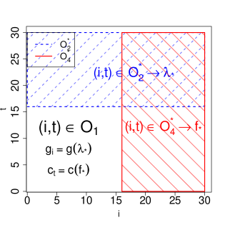
Figure 1: Sample split for partition 1

Figure 1 details an example of this sample splitting technique for clustering within partition $\mathcal{O}_{1}$. Here we see clearly how the partitions for proxy estimation $\mathcal{O}^{*}_{2}$ and $\mathcal{O}^{*}_{4}$ do not overlap with the partition we are grouping within, $\mathcal{O}_{1}$. This guarantees that we do not introduce any dependence between the group functions and the noise term by making sure grouping within each partition is not a function of the independent noise term, $\varepsilon_{it}$, from observations within that partition. This becomes important in our derivations in Section 4.2, where we require that the process $X_{it}\,\varepsilon_{it}$ remains zero mean and independently distributed after group means are projected out.

With these cluster assignments it then becomes straightforward to estimate (9) by first taking within-cluster mean-differences for each partition and then simply apply pooled OLS on the transformed variables.

Notice that by allowing the partitioning in (11) used to estimate proxy variables to extend over the whole sample of either $N$ or $T$, we get better estimates than just using the original partition (10). As discussed earlier, it is crucial to avoid poor initial estimates of proxy variables to better approximate the residual terms in the Taylor expansion in expression (8).

3 Asymptotic results for the least squares estimator

Here, we derive convergence rate results for the least-squares estimator (5) for a data generating process given by (1). Thus, we generalize the consistency results in Bai (2009) and Moon and Weidner (2015) to the case where the underlying panel regression model does not satisfy the factor model in (4). However, as explained in the introduction, the factor model in (4) can be viewed as an approximation of (1), and this approximation idea can be formalized asymptotically, as long as we allow the number of factors $R=R_{NT}$ used in the least-squares estimator (5) to grow with $N$ and $T$.

3.1 Consistency and convergence rate

From now on, we denote the true parameter $\beta$ that generates the data by $\beta^{0}$. We rewrite model (1) as

$$Y_{it} =X_{it}^{\prime}\,\beta^{0}+\Gamma_{it}+\varepsilon_{it},$$ (13)

where both $\Gamma_{it}$ and $\varepsilon_{it}$ are unobserved. Our main convergence rate results in Theorem 1 actually hold for any $N\times T$ matrix $\Gamma=(\Gamma_{it})$ that satisfies Assumption 4 below, but ultimately we are of course interested in the case $\Gamma_{it}=h(\alpha_{i},\gamma_{t})$. Arbitrary dependence between $X_{it}$ and $\Gamma_{it}$ is allowed for, so there is a potential endogeneity problem.

Remember that the components of the $K$-vector $X_{it}$ are denoted by $X_{it,k}$, $k=1,\ldots,K$. Let $X_{k}=(X_{it,k})$ and $\varepsilon=(\varepsilon_{it})$ be $N\times T$ matrices. For a matrix $A$ we denote $r$’th largest singular value by $\sigma_{r}(A)$, that is, $\sigma^{2}_{r}(A)$ is equal to the $r$’th largest eigenvalue of $AA^{\prime}$. Furthermore, for matrices we denote the spectral norm by $\|\cdot\|$, and for vectors the norm $\|\cdot\|$ denotes the Euclidean norm. We write wpa1 for “with probability approaching one”. We impose the following assumptions.

Assumption 1 (Bounded norms of $X_{k}$ and $\varepsilon$).

• $\displaystyle\frac{1}{NT}\sum_{i=1}^{N}\sum_{t=1}^{T}(X_{it,k})^{2}={O}_{P}(1)$,  for $k=1,\ldots,K$.

• $\displaystyle\|\varepsilon\|={O}_{P}\left(\sqrt{\max\{N,T\}}\right)$.

Assumption 2 (Weak Exogeneity of $X_{k}$).

$\displaystyle\sum_{i=1}^{N}\sum_{t=1}^{T}X_{it,k}\varepsilon_{it}={O}_{P}(\sqrt{NT})$, for $k=1,\ldots,K$.

Assumption 3 (Non-Collinearity of $X_{k}$).

Consider linear combinations $\delta\cdot X:=\sum_{k=1}^{K}\delta_{k}X_{k}$ of the regressors $X_{k}$ with vectors $\delta\in\mathbb{R}^{K}$ such that $\|\delta\|=1$. Assume that there exists a constant $b>0$ such that

$$\min_{\{\delta\in\mathbb{R}^{K},\,\|\delta\|=1\}}\,\sum_{r=2R_{NT}+1}^{\min(N,T)}\,\sigma^{2}_{r}\left[\frac{(\delta\cdot X)}{\sqrt{NT}}\right]\; \geq b\;,\qquad\text{wpa1.}$$

Assumption 4 (Singular value decay).

There exists a constant $\rho>3/2$ such that

$$\frac{1}{NT}\sum_{r=R_{NT}+1}^{\min(N,T)}\sigma^{2}_{r}(\Gamma)=O_{P}\left(R_{NT}^{1-2\rho}\right).$$

Here, $R=R_{NT}$ is the number of factors that is chosen in the computation of the least-squares estimator $\widehat{\beta}_{\,\rm LS}$ in (5). We require $R_{NT}\rightarrow\infty$ as $N,T\rightarrow\infty$ to obtain consistency of $\widehat{\beta}_{\,\rm LS}$.

Lemma 1 below justifies Assumption 4 for our main case of interest $\Gamma_{it}=h(\alpha_{i},\gamma_{t})$, and we therefore postpone the discussion of that assumption until we discuss that lemma. Assumptions 1-3 are very similar to the assumptions used in Bai (2009) and Moon and Weidner (2015) to show consistency of $\widehat{\beta}_{\,\rm LS}$, and the following discussion of those assumptions will, accordingly, be brief.

Assumption 1(i) follows from Markov’s inequality as long as the second moment of $X_{it,k}$ is uniformly bounded. Assumption 1(ii) follows, for example, from the inequality in Latala (2005) if $\varepsilon_{it}$ has mean zero, uniformly bounded fourth moment, and is independent across $i$ and $t$. However, the assumption still holds if $\varepsilon_{it}$ is weakly correlated across $i$ and over $t$, see Moon and Weidner (2015). Assumption 2 is satisfied as long as $X_{it}\varepsilon_{it}$ has zero mean, uniformly bounded second moment, and is weakly correlated across $i$ and over $t$.

To understand Assumption 3, notice first that for $R_{NT}=0$ the expression $\sum_{r}\,\sigma^{2}_{r}\left[\frac{(\delta\cdot X)}{\sqrt{NT}}\right]$ in that assumption becomes

$$\sum_{r=1}^{\min(N,T)}\,\sigma^{2}_{r}\left[\frac{(\delta\cdot X)}{\sqrt{NT}}\right]=\frac{1}{NT}\sum_{i=1}^{N}\sum_{t=1}^{T}(\delta\cdot X)_{it}^{2}.$$

Thus, for $R_{NT}=0$, the assumption is just a standard non-collinearity assumption on the regressors, which demands that every non-trivial linear combination $\delta\cdot X$ of the regressors has sufficient variation. Next, for $R_{NT}>0$ we have

$$\sum_{r=2R_{NT}+1}^{\min(N,T)}\,\sigma^{2}_{r}\left[\frac{(\delta\cdot X)}{\sqrt{NT}}\right]=\frac{1}{NT}\sum_{i=1}^{N}\sum_{t=1}^{T}(\delta\cdot X)_{it}^{2}-\sum_{r=1}^{2R_{NT}}\,\sigma^{2}_{r}\left[\frac{(\delta\cdot X)}{\sqrt{NT}}\right],$$

that is, the assumption demands that the variation in the linear combination $\delta\cdot X$ does not only come from the leading $2R_{NT}$ singular values of this linear combination.

Of course, if ${\rm rank}(\delta\cdot X)\leq 2R_{NT}$, then for $r>2R_{NT}$ all the singular values $\sigma_{r}\left(\delta\cdot X\right)$ are equal to zero and the assumption is violated. Thus, a necessary condition for Assumption 3 is that ${\rm rank}(\delta\cdot X)>2R_{NT}$, that is, any linear combination of the regressors needs to be a “high-rank matrix”. For example, a constant regressor $X_{it,1}=1$ violates this assumption (it constitutes a rank one matrix, which could be easily absorbed into the unobserved $\Gamma_{it}$), but if the regressors are drawn from a DGP with random variation across both $i$ and $t$, then they typically have full rank. Again, we refer to the existing papers on the least-squares estimator with interactive fixed effects for further discussion of this generalized non-collinearity condition on the regressors.

Theorem 1 (Consistency of $\widehat{\beta}_{\,\rm LS}$).

Let Assumptions 1 – 4 hold, and furthermore assume that $R_{NT}=o(\min\{N,T\})$ as $N,T\rightarrow\infty$. Then we have

$$\widehat{\beta}_{\,\rm LS}-\beta^{0}=O_{P}\Big{(}R_{NT}^{(3-2\rho)/2}\Big{)}+O_{P}\Big{(}R_{NT}\,(\min\{N,T\})^{-1/2}\Big{)}.$$ (14)

Therefore, by choosing $R_{NT}\propto(\min\{N,T\})^{\frac{1}{2\rho-1}}$ we obtain that

$$\widehat{\beta}_{\,\rm LS}-\beta^{0}={O}_{P}\Big{(}\min\{N,T\}^{\frac{3-2\rho}{2(2\rho-1)}}\Big{)}.$$

Assumption 4 demands $\rho>3/2$, and the first term on the right-hand side of (14) is therefore decreasing in the number of factors $R_{NT}$ used for estimation. By contrast, the second term on the right-hand side of (14) is increasing in $R_{NT}$. The final part of the theorem simply gives the rate for $R_{NT}$ that optimally balances the trade-off between those two terms. This is analogous the bias-variance trade-off for bandwidth selection in non-parametric estimation. Indeed, the term $O_{P}\left(R_{NT}^{(3-2\rho)/2}\right)$ is due to the approximation error of the $N\times T$ matrix $\Gamma$ (which can have full rank) by only a finite number of factors (of rank only $R_{NT}$). As expected, the approximation error is small when choosing a more flexible model (large $R_{NT}$).

The second term on the right-hand side of (14) also occurs when one considers a conventional interactive fixed effect model, where the true matrix $\Gamma$ itself is assumed to have low rank and the approximation error is therefore not present (for $R_{NT}\geq{\rm rank}(\Gamma)$). For that case, the first paper to derive the large $N$, $T$ asymptotic properties for $\widehat{\beta}_{\,\rm LS}$ was Bai (2009). He imposes assumptions (in particular, $R_{NT}={\rm rank}(\Gamma)={\rm constant}$, and all factors in $\Gamma$ are “strong factors”) that are strong enough to derive the result $\widehat{\beta}_{\,\rm LS}-\beta^{0}=O_{P}(1/\sqrt{NT})$ when $N$ and $T$ grow at the same rate. However, without such strong assumptions, the estimator $\widehat{\beta}_{\,\rm LS}$ may very well converge at a slower rate. For example, in Section 4.3 of Moon and Weidner (2015) a concrete data generating process is given for which $\widehat{\beta}_{\,\rm LS}$ only converges at the slower rate $(\min\{N,T\})^{-1/2}$. The key difference between that example and Bai (2009) is that $R_{NT}>{\rm rank}(\Gamma)$, that is, the number of factors in the estimation is larger than the true number of factors. More generally, as soon as the “strong factor” assumption or the known number of factors assumption ($R_{NT}={\rm rank}(\Gamma)$) are violated, there is no guarantee that $\widehat{\beta}_{\,\rm LS}$ converges at the fast rate derived in Bai (2009). In the absence of those assumptions, Theorem 4.1 in Moon and Weidner (2015) shows that $\widehat{\beta}_{\,\rm LS}-\beta^{0}=O_{P}\Big{(}(\min\{N,T\})^{-1/2}\Big{)}$ when $R_{NT}\geq{\rm rank}(\Gamma)$ is fixed. The second term on the right-hand side of (14) exactly generalizes that rate to the case where $R_{NT}$ is allowed to grow asymptotically.

In our setting, we cannot impose the “strong factor” or known number of factor assumptions in Bai (2009), because, as explained in the introduction, the data generating process $\Gamma_{it}=h(\alpha_{i},\gamma_{t})$ typically generates an infinite sequence of factors of decreasing strength. Demanding all those factors in equation (3) to be strong factors makes no sense in our setting. Deriving a convergence rate for $\widehat{\beta}_{\,\rm LS}$ faster than $(\min\{N,T\})^{-1/2}$ in our model therefore appears to very challenging, to say the least. This is of course, the key motivation for why we also consider the two-way grouped fixed effect estimator in this paper, see Section 4 below.

Remark 1.

If we change Assumption 4 to

$$\sigma_{r}(\Gamma)\,\leq\,c\,\sqrt{NT}\,r^{-\rho},$$ (15)

for all $r\in\{R_{NT}+1,\dots\min\{N,T\}\}$, wpa1, and some constant $c>0$, then the result in equation (14) of Theorem 1 can be improved to

$$\widehat{\beta}_{\,\rm LS}-\beta^{0}={O}_{P}\left({R_{NT}^{\,1-\rho}}\right)+{O}_{P}\left({R_{NT}}\,{(\min\{N,T\})^{-1/2}}\right),$$

and we can then obtain consistency of $\widehat{\beta}$ under the weaker condition $\rho>1$. Condition (15) implies Assumption 4, but not vice versa, because Assumption 4 is a condition on the sum of the squared singular values, not on each of the singular values separately. It turns out to be technically much easier to verify Assumption 4 than to verify (15) for our main case of interest $\Gamma_{it}=h(\alpha_{i},\gamma_{t})$, as we do in Lemma 1 below. This explains why we have chosen that formulation of the assumption and theorem in our baseline presentation.

Despite the technical subtleties explained in the preceding remark, one should still interpret Assumption 4 as imposing a particular decay rate for the singular values $\Gamma$, as in display (15) of the remark. Thus, the leading few singular value can have a magnitude of $\sqrt{NT}$, as would be the case under the “strong factor assumption” in the usual interactive fixed effects model of Bai (2009). However, as $N$, $T$, $r$ all converge to infinity we require the $\sigma_{r}(\Gamma)$ to converge at the polynomial rate $r^{-\rho}$ in order to satisfy the summability condition in Assumption 4.

The results in this section so far have not made any use of the structure $\Gamma_{it}=h(\alpha_{i},\gamma_{t})$. Theorem 1 is applicable to any other data generating process for $\Gamma$ that satisfies Assumption 4. A full-rank matrix $\Gamma$ satisfying that assumption could, for example, also be generated by a dynamic factor model (see e.g. Forni, Hallin, Lippi and Reichlin 2000, 2005, Stock and Watson 2002).

In the following we now focus exclusively on the case $\Gamma_{it}=h(\alpha_{i},\gamma_{t})$. The following lemma provides conditions on the function $h(\cdot,\cdot)$ that guarantee that Assumption 4 is satisfied.

Lemma 1.

Assume $\alpha_{i}\in\Omega_{\alpha}$ and $\gamma_{t}\in\Omega_{\gamma}$, and that $h:\Omega_{\alpha}\times\Omega_{\gamma}\rightarrow\mathbb{R}$ is $p$ times continuously differentiable in both arguments, with uniformly bounded mixed-derivatives up to order $p$, and the domains $\Omega_{\alpha}\subset\mathbb{R}^{n_{\alpha}}$ and $\Omega_{\gamma}\subset\mathbb{R}^{n_{\gamma}}$ are smooth and bounded. Then for $\Gamma_{it}=h(\alpha_{i},\gamma_{t})$ Assumption 4 is satisfied for $R_{NT}\rightarrow\infty$ with $\rho=\frac{p}{\min\left\{n_{\alpha},n_{\gamma}\right\}}$.

Here, we measure the smoothness of the function $h(\cdot,\cdot)$ by $p$, which is the number of times it is continuously differentiable. The decay rate $\rho$ of the singular values of $\Gamma$ then depends on this measure of smoothness and the dimensions $n_{\alpha}$ and $n_{\gamma}$ of the arguments $\alpha_{i}$ and $\gamma_{t}$. The smoother the function $h(\cdot,\cdot)$, for fixed dimensions $n_{\alpha}$ and $n_{\gamma}$, the faster the eigenvalues of $\Gamma$ converge to zero.

The proof of Lemma 1 crucially relies on the functional singular value decomposition in (2) and results on the decay rate of the corresponding singular values in Griebel and Harbrecht (2014). The only technical contribution of the proof is then to properly relate those known results on the functional singular value to the matrix singular values of $\Gamma$.

Notice that Lemma 1 requires no assumptions on the data generating process of $\alpha_{i}$ and $\gamma_{t}$, apart from boundedness of the domains $\Omega_{\alpha}$ and $\Omega_{\gamma}$, which can always be achieved by a reparameterization. Thus, those nuisance parameters can be arbitrarily correlated with each other (across $i$ and over $t$) and with the regressors $X_{it,k}$. This result is analogous to the consistency Theorem 4.1 for $\widehat{\beta}_{\,\rm LS}$ in Moon and Weidner (2015), where also no assumptions on the interactive fixed effects are imposed at all, apart from ${\rm rank}(\lambda f^{\prime})\leq R$.

From Theorem 1 and Lemma 1 we have the following corollary.

Corollary 1.

Let Assumptions 1 – 3 and the assumption on $h(.,.)$ in Lemma 1 be satisfied with $p>3\min\left\{n_{\alpha},n_{\gamma}\right\}/2$, and also let $R_{NT}\rightarrow\infty$ such that ${R_{NT}/(\min\{N,T\})^{1/2}\rightarrow 0}$. Then we have

$$\widehat{\beta}_{\,\rm LS}-\beta^{0}=o_{P}(1).$$

This is our final consistency result for the least-squares estimator of Bai (2009) in a data generating process given by (1). The convergence rate of the estimator was already discussed after Theorem 1 above, in particular, the difficulty in showing a convergence rate faster than $(\min\{N,T\})^{1/2}$ in our setting.

3.2 Further discussion

Here, we want to present some further intuition on the formal results on $\widehat{\beta}_{\,\rm LS}$ presented above. The discussion in this subsection is purely heuristic and does not aim to provide any formal derivations.

Remember the functional singular value decomposition in equation (2) of the introduction, which we now write as $h(\alpha_{i},\gamma_{t})=\sum_{r=1}^{\infty}\lambda^{0}_{ir}\,f^{0}_{tr}$. For the sake of the following discussion, suppose that variation from $h(\alpha_{i},\gamma_{t})$ dominates the variation in $X_{it}^{\prime}\,\beta$ and $\varepsilon_{it}$ for the leading $R_{NT}$ principal components of the residuals $Y_{it}-X_{it}^{\prime}\,\beta-\sum_{r=1}^{R}{\lambda}_{ir}\,{f}_{tr}=\sum_{r=1}^{\infty}\lambda^{0}_{ir}\,f^{0}_{tr}-X_{it}^{\prime}\,(\beta-\beta^{0})+\varepsilon_{it}$. In this “best case scenario”, the estimated factors $\sum_{r=1}^{R}{\lambda}_{ir}\,{f}_{tr}$ in the definition of $\widehat{\beta}_{\rm LS}$ in (5) will coincide with the leading $R_{NT}$ components $\sum_{r=1}^{R}{\lambda}^{0}_{ir}\,{f}^{0}_{tr}$ of $h(\alpha_{i},\gamma_{t})$, and we then have

$$\widehat{\beta}_{\rm LS}-\beta^{0}=\zeta_{NT}+\xi_{NT},$$

where

$$\zeta_{NT} =\left(\frac{1}{NT}\sum_{i=1}^{N}\sum_{t=1}^{T}X^{\prime}_{it}\,X_{it}\right)^{-1}\frac{1}{NT}\sum_{i=1}^{N}\sum_{t=1}^{T}X^{\prime}_{it}\,\varepsilon_{it}$$

$$\xi_{NT} =\left(\frac{1}{NT}\sum_{i=1}^{N}\sum_{t=1}^{T}X^{\prime}_{it}\,X_{it}\right)^{-1}\frac{1}{NT}\sum_{i=1}^{N}\sum_{t=1}^{T}X^{\prime}_{it}\,\sum_{r=R+1}^{\infty}\lambda^{0}_{ir}f^{0}_{tr}.$$

Under standard regularity conditions we have $\sqrt{NT}\zeta_{NT}\Rightarrow{\cal N}(0,\Sigma)$, and under the assumptions in the last subsection we have $\xi_{NT}={O}_{P}\Big{(}R_{NT}^{(3-2\rho)/2}\Big{)}$. In this “best-case scenario” we can therefore have $R_{NT}\rightarrow\infty$ quick enough such that $\xi_{NT}=o_{P}(1/\sqrt{NT})$.

However, this is not a realistic scenario for $R_{NT}\rightarrow\infty$, because as $R_{NT}$ grows, eventually the singular values of $\varepsilon_{it}$ will dominate those of $\sum_{r=R+1}^{\infty}\lambda^{0}_{ir}f^{0}_{tr}$, and the factor projection method will just project out idiosyncratic noise, or even contributions from $X_{it}^{\prime}\,(\widehat{\beta}_{\rm LS}-\beta^{0})$. This implies that the problematic variation associated with $\lambda^{0}_{ir}f^{0}_{tr}$ for most singular values $r$ remains. This explains why it is so difficult to show anything better than the convergence rate results in Theorem 1 for the estimator $\widehat{\beta}_{\rm LS}$ in our setting.

4 Asymptotic results for the group fixed-effect estimator

The main goal of this section is to derive asymptotic results for the estimator $\widehat{\beta}_{\rm GS}$ defined in (9), which is the sample-splitting version of the group fixed-effect estimator. But we are first going to discuss the initial group fixed-effect estimator $\widehat{\beta}_{\rm G}$ defined in (7) without sample-splitting. We will not actually derive convergence rate results for $\widehat{\beta}_{\rm G}$ itself, but the discussion of the approximation bias of $\widehat{\beta}_{\rm G}$ will be a very useful precursor of the results for $\widehat{\beta}_{\rm GS}$.

4.1 Results for $\widehat{\beta}_{\rm G}$

We can rewrite our estimating equation for the group fixed-effect estimator in (6) as

$$Y =X\cdot\beta+\delta\,D_{\delta}^{\prime}+D_{\nu}\,\nu^{\prime}+\varepsilon,$$ (16)

where $\delta$ and $\nu$ are the $N\times C$ and $T\times G$ matrices of nuisance parameters, while $D_{\delta}$ and $D_{\nu}$ are $T\times C$ and $N\times G$ are binary matrices in which each row contains a single one, indicating the group membership of the corresponding unit or time period, respectively. By standard partitioned regression results we can then rewrite the group fixed-effect estimator in (7) as

$$\widehat{\beta}_{\rm G} =\left(\sum_{i=1}^{N}\sum_{t=1}^{T}\widetilde{X}_{it}^{\prime}\,\widetilde{X}_{it}\right)^{-1}\sum_{i=1}^{N}\sum_{t=1}^{T}\widetilde{X}_{it}^{\prime}\,\widetilde{Y}_{it}, \widetilde{X}_{k} =M_{N}\,X_{k}\,M_{T}, \widetilde{Y} =M_{N}\,Y\,M_{T},$$ (17)

where $\widetilde{X}_{it}=\left(\widetilde{X}_{it,1},\ldots,\widetilde{X}_{it,K}\right)$, $\widetilde{Y}_{it}$ and $\widetilde{X}_{it,k}$ are the entries of the $N\times T$ matrices $\widetilde{X}_{k}$ and $\widetilde{Y}$, respectively, and $M_{N}=\mathbb{I}_{N}-D_{\nu}(D_{\nu}^{\prime}D_{\nu})^{-1}D_{\nu}^{\prime}$ and $M_{T}=\mathbb{I}_{T}-D_{\delta}(D_{\delta}^{\prime}D_{\delta})^{-1}D_{\delta}^{\prime}$ are projection matrices of dimesion $N\times N$ and $T\times T$, respectively.

Using this representation of the group fixed-effect estimator and the model in (13) we obtain that

$$\widehat{\beta}_{\rm G}-\beta^{0} =\phi_{NT}+\kappa_{NT},$$ (18)

where

$$\phi_{NT} :=\left(\sum_{i=1}^{N}\sum_{t=1}^{T}\widetilde{X}_{it}^{\prime}\widetilde{X}_{it}\right)^{-1}\sum_{i=1}^{N}\sum_{t=1}^{T}\widetilde{X}_{it}^{\prime}\,\varepsilon_{it}, \kappa_{NT} :=\left(\sum_{i=1}^{N}\sum_{t=1}^{T}\widetilde{X}_{it}^{\prime}\widetilde{X}_{it}\right)^{-1}\sum_{i=1}^{N}\sum_{t=1}^{T}\widetilde{X}_{it}^{\prime}\,\widetilde{\Gamma}_{it},$$ (19)

with $\widetilde{\Gamma}$ defined analogously to $\widetilde{X}_{k}$ and $\widetilde{Y}$ in (17). In the definition of $\phi_{NT}$ we can equivalently write $\widetilde{\varepsilon}_{it}$ instead of $\varepsilon_{it}$, but since $M_{N}$ and $M_{T}$ are idempotent matrices, and $\widetilde{X}_{it}$ is already the projected regressor, this does not matter. The same is true, of course, for $\widetilde{\Gamma}_{it}$ vs $\Gamma_{it}$ in the definition of $\kappa_{NT}$. However, the expressions in (19) turn out to be convenient as written.

Here, $\kappa_{NT}$ is the approximation error of having replaced the nonlinear specification $\Gamma_{it}=h(\alpha_{i},\gamma_{t})$ in our model in (1) by the much simpler additive specification $\delta_{i,c_{t}}+\nu_{t,g_{i}}$ in the estimation equation (6). To see this, we can use standard matrix inequalities to bound the Euclidian norm of $\kappa_{NT}$ by

$$\left\|\kappa_{NT}\right\| \leq\left\|\left(\sum_{i=1}^{N}\sum_{t=1}^{T}\widetilde{X}_{it}^{\prime}\widetilde{X}_{it}\right)^{-1}\right\|\left(\max_{k}\left\|\widetilde{X}_{k}\right\|_{F}\right)\,\big{\|}\widetilde{\Gamma}\big{\|}_{F},$$ (20)

where $\|\cdot\|_{F}$ refers to the Frobenius norm. Due to the definition of $M_{N}$ and $M_{T}$ we have

$$\big{\|}\widetilde{\Gamma}\big{\|}^{2}_{F}=\min_{\delta\in\mathbb{R}^{N\times C}}\,\min_{\nu\in\mathbb{R}^{T\times G}}\,\sum_{i=1}^{N}\sum_{t=1}^{T}\left[h(\alpha_{i},\gamma_{t})-\delta_{i,c_{t}}-\nu_{t,g_{i}}\right]^{2}.$$ (21)

The last two displays show that $\kappa_{NT}$ is small whenever $h(\alpha_{i},\gamma_{t})$ can be well approximated by $\delta_{i,c_{t}}+\nu_{t,g_{i}}$. In equation (8) we already informally discussed the magnitude of this approximation error, and found that it is of order $\|\alpha_{i}-\overline{\alpha}_{g_{i}}\|^{2}+\|\gamma_{t}-\overline{\gamma}_{c_{t}}\|^{2}$. We now want to provide a more formal discussion of this and show that $\kappa_{NT}$ is asymptotically small under appropriate regularity conditions.

In Section 2.2.2 we described the clustering algorithms that delivers the group memberships $g_{i}$ and $c_{t}$ based on the initial estimates $\widehat{\lambda}^{*}_{i}$ and $\widehat{f}^{*}_{t}$. The goal of the clustering is to group units $i$ with approximately the same value of $\alpha_{i}$, and to group time periods $t$ with approximately the same $\gamma_{t}$. It is therefore crucial that $\widehat{\lambda}^{*}_{i}$ and $\widehat{f}^{*}_{t}$ are good proxies for $\alpha_{i}$ and $\gamma_{t}$. Specifically, we require that there exist functions $\lambda^{*}:{\cal A}\rightarrow\mathbb{R}^{R_{*}}$ and $f^{*}:{\cal C}\rightarrow\mathbb{R}^{R_{*}}$ such that $\widehat{\lambda}^{*}_{i}$ and $\widehat{f}^{*}_{t}$ converge to the non-random limits $\lambda^{*}(\alpha_{i})$ and $f^{*}(\gamma_{t})$ as $N,T\rightarrow\infty$. The following assumption formalizes this and states all the regularity condition that we require on $h(\cdot,\cdot)$, $\lambda^{*}(\cdot)$, $f^{*}(\cdot)$, $\widehat{\lambda}^{*}_{i}$, $\widehat{f}^{*}_{t}$, and $X_{it}$.

Assumption 5.

There exists a sequence $\xi_{NT}>0$ such that $\xi_{NT}\to 0$ as $N,T\to\infty$, and

1. The function $h(\cdot,\cdot)$ is at least twice continuously differentiable with uniformly bounded second derivatives.

2. Every unit $i$ is a member of exactly one group $g_{i}\in\{1,\ldots,G\}$, and every time period $t$ is a member of exactly one group $c_{t}\in\{1,\ldots,C\}$. The size of all $G$ groups of units, and the size of all $C$ groups of time periods is bounded uniformly by $Q_{\max}$.

3. There exists $B>0$ such that $\left\|a-b\right\|\leq B\left\|\lambda^{*}(a)-\lambda^{*}(b)\right\|$ for all $a,b\in{\cal A}$ , and $\left\|a-b\right\|\leq B\left\|f^{*}(a)-f^{*}(b)\right\|$ for all $a,b\in{\cal C}$, and the domains ${\cal A}$ and ${\cal C}$ are convex set.

4. $\frac{1}{N}\sum_{i=1}^{N}\left(\left\|\widehat{\lambda}^{*}_{i}-\lambda^{*}(\alpha_{i})\right\|^{2}\right)=O_{P}\left(\xi_{NT}\right)$,   $\frac{1}{T}\sum_{t=1}^{T}\left(\left\|\widehat{f}^{*}_{t}-f^{*}(\gamma_{t})\right\|^{2}\right)=O_{P}\left(\xi_{NT}\right)$.

5. $\frac{1}{N}\sum_{i=1}^{N}\left\|\widehat{\lambda}^{*}_{i}-\widehat{\lambda}^{*}_{j(i)}\right\|^{2}=O_{P}\left(\xi_{NT}\right)$ for any matching function $j(i)\in\{1,\ldots,N\}$ such that $g_{i}=g_{j(i)}$, and $\frac{1}{T}\sum_{t=1}^{T}\left\|\widehat{f}^{\,*}_{t}-\widehat{f}^{\,*}_{s(t)}\right\|^{2}=O_{P}\left(\xi_{NT}\right)$ for any matching function $s(t)\in\{1,\ldots,T\}$ such that $c_{t}=c_{s(t)}$.

6. $\max_{k,i,t}\left|\widetilde{X}_{it,k}\right|=O_{P}(1)$, and $\operatorname*{plim}_{N,T\rightarrow\infty}\frac{1}{{NT}}\sum_{i=1}^{N}\sum_{t=1}^{T}\widetilde{X}_{it}^{\prime}\widetilde{X}_{it}=\Omega$, where $\Omega$ is a positive definite non-random matrix.

Lemma 2.

Under Assumption 5 we have

$$\kappa_{NT}=O_{P}(\xi_{NT})$$

The lemma shows that the approximation error $\kappa_{NT}$ vanishes at rate $\xi_{NT}$ as $N,T\rightarrow\infty$. The assumption and lemma are formulated for arbitrary rates, but as will become clear from the following discussion, the best we can achieve in our setting is a rate of $\xi_{NT}=1/\min(N,T)$, which coincides with $\xi_{NT}=1/\sqrt{NT}$ in the special case that $N$ and $T$ grow at the same rate.

Part (i) of Assumption 5 requires the function $h(\cdot,\cdot)$ to be sufficiently smooth. This condition should not be surprising, because our informal discussion of the approximation error in equation (8) already relies on a second order Taylor expansion of $h(\cdot,\cdot)$, and the proof of Lemma 2 is based on exactly such an expansion.

Part (iii) and (iv) of the assumption are analogous to “Assumption 2 (injective moments)” in Bonhomme, Lamadon and Manresa (2021), except that they consider a one-way fixed effect setting while we consider a two-way fixed effect setting. Part (iii) requires the functions $\lambda^{*}(\cdot)$ and $f^{*}(\cdot)$ to be injective, that is, $\alpha_{i}$ and $\gamma_{t}$ can be uniquely recovered from knowing $\lambda^{*}(\alpha_{i})$ and $f^{*}(\gamma_{t})$. A necessary condition for this is that

$$R^{*}\geq\max(d_{\alpha},d_{\gamma}),$$ (22)

where $d_{\alpha}$ and $d_{\gamma}$ are the dimensions of $\alpha_{i}$ and $\gamma_{t}$, respectively. Part (iv) requires the estimates $\widehat{\lambda}^{*}_{i}$ and $\widehat{f}^{*}_{t}$ to converge to $\lambda^{*}(\alpha_{i})$ and $f^{*}(\gamma_{t})$ at the average rate of $\xi_{NT}^{1/2}$. We expect that the estimated eigenfunctions of $h(\alpha_{i},\gamma_{t})$, which correspond to the estimated factor loadings and factors, proposed as cluster proxies in Section 2.2.2 satisfy this assumption by an application of Theorem 1 from Bai and Ng (2002). Since $T$ observations are available for unit $i$ we expect that $\widehat{\lambda}^{*}_{i}$ converges at a rate of $T^{1/2}$, and since $N$ observations are available for time period $t$ we expect that $\widehat{f}^{*}_{t}$ converges at a rate of $N^{1/2}$, see also, for example, Theorem 1 and 2 in Bai (2003). This explains why $\xi_{NT}=1/\min(N,T)$ is the best rate we can achieve here.

Part (v) of Assumption 5 is a high-level assumption on the clustering mechanism used to obtain the group memberships $g_{i}$ and $c_{t}$. For units $i$ and $j$ in the same group, and for time periods $t$ and $s$ in the same group, we demand the average differences $\widehat{\lambda}^{*}_{i}-\widehat{\lambda}^{*}_{j}$ and $\widehat{f}^{\,*}_{t}-\widehat{f}^{\,*}_{s}$ to be small as $N,T\rightarrow\infty$. In other words, we require that the clustering mechanism does what it is intended to do, namely forming groups such that the estimates $\widehat{\lambda}^{*}_{i}$ and $\widehat{f}^{\,*}_{t}$ for units $i$ and time periods $t$ in the same group are close to each other. For a given clutstering algorithms (e.g. the one describe in Section 2.2.2) one could prove that this assumption holds under further regularity conditions on the distribution of $\alpha_{i}$ and $\gamma_{t}$, see, for example, Lemma 1 in Bonhomme, Lamadon and Manresa 2021. In particular, a necessary condition for part (v) of Assumption 5 to hold is the following:

Regularity condition.

$\frac{1}{N}\sum_{i=1}^{N}\left\|\alpha_{i}-\alpha_{j(i)}\right\|^{2}=O_{P}\left(\xi_{NT}\right)$ for any matching function $j(i)\in\{1,\ldots,N\}$ such that $g_{i}=g_{j(i)}$, and $\frac{1}{T}\sum_{t=1}^{T}\left\|\gamma_{t}-\gamma_{s(t)}\right\|^{2}=O_{P}\left(\xi_{NT}\right)$ for any matching function $s(t)\in\{1,\ldots,T\}$ such that $c_{t}=c_{s(t)}$.

This condition coincides with Assumption 5(v) in the unrealistic case that $\widehat{\lambda}^{*}_{i}=\alpha_{i}$ and $\widehat{f}^{\,*}_{t}=\gamma_{t}$. Starting from this unrealistic case and then applying the transformations $\lambda^{*}:{\cal A}\rightarrow\mathbb{R}^{R_{*}}$ and $f^{*}:{\cal C}\rightarrow\mathbb{R}^{R_{*}}$ and adding noise to the estimates then gives part (v) of Assumption 5. Crucially, for this regularity condition to hold, we need that $\xi_{NT}\gtrsim 1/\min(N^{2/d_{\alpha}},T^{2/d_{\gamma}})$, see Lemma 2 in Bonhomme, Lamadon and Manresa (2021) for the analogous results in a one-way fixed effect model (also Graf and Luschgy 2002). Since our actual clustering method is not based on the unobserved $\alpha_{i}$ and $\gamma_{t}$, but on $\widehat{\lambda}^{*}_{i}$ and $\widehat{f}^{\,*}_{t}$ we require the stronger condition (in view of (22)) that

$$\xi_{NT}\gtrsim[\min(N,T)]^{-2/R^{*}}.$$

This is a necessary condition for Assumption 5(v) to be satisfied. Therefore, if we want to achieve the best possible rate $\xi_{NT}=1/\min(N,T)$, then we need $R^{*}\leq 2$, which according to (22) implies that $d_{\alpha}\leq 2$ and $d_{\gamma}\leq 2$. This discussion shows that our group fixed-effect estimator $\widehat{\beta}_{\rm G}$ suffers from a curse of dimensionality with regards to the dimensions of $\alpha_{i}$ and $\gamma_{t}$. However, this should be unsurprising, given the semi-parametric nature of the estimation problem – with non-parametric component $h(\alpha_{i},\gamma_{t})$. This also shows that there is a tradeoff between the LS estimator analyzed in Section 3 and the group fixed effects estimator discussed here – we will further compare those two estimators in our MC analysis below.

Finally, part (vi) of Assumption 5 requires some regularity conditions on the projected regressors $\widetilde{X}_{k}=M_{N}\,X_{k}\,M_{T}$ defined in (17).

This concludes our discussion of the approximation error $\kappa_{NT}$. We have argued that, under appropriate regularity conditions, including $\max(d_{\alpha},d_{\gamma})\leq 2$, we can use Lemma 2 to obtain $\kappa_{NT}=1/\sqrt{NT}$, for $N$ and $T$ growing to infinity at the same rate. Since $\widehat{\beta}_{\rm G}-\beta^{0}=\phi_{NT}+\kappa_{NT}$ we could then conclude that $\widehat{\beta}_{\rm G}-\beta^{0}=O_{P}(1/\sqrt{NT})$, if we could also show that $\phi_{NT}=O_{P}(1/\sqrt{NT})$.

From the definition of $\phi_{NT}$ in (19) one might think that it is easy to derive this result on $\phi_{NT}$ by imposing an approximate exogeneity condition on the regressors. However, the problem is that $\widetilde{X}_{k}$ depends on the group assignments of units $i$ and time periods $t$, which were constructed based on $\widehat{\lambda}^{*}$ and $\widehat{f}^{*}$, which depend on the errors $\varepsilon$. Thus, $\widetilde{X}_{k}$ depends on $\varepsilon$ in complicated ways through the group assignment, making a proof of $\phi_{NT}=O_{P}(1/\sqrt{NT})$ technically challenging. In principle, we expect that

$$\sqrt{NT}\,\phi_{NT}\Rightarrow{\cal N}(0,\Sigma_{\rm G})$$ (23)

holds for an appropriate covariance matrix $\Sigma_{\rm G}$, and our simulations evidence suggest that this is indeed the case. However, we are not aiming to prove this result in this paper. As explained already in Section 2, this technical difficulty in analyzing $\widehat{\beta}_{\rm G}$ is exactly why we introduced the split-sample version of the group fixed-effect estimator, for which we are going to derive results in the following.

4.2 Results for $\widehat{\beta}_{\rm GS}$

The split-sample version of the group fixed effect estimator was introduced in Section 2.2.3 above. Using the Frisch-Waugh-Lovell theorem we can rewrite $\widehat{\beta}_{\rm GS}$ in equation (9) as follows:

$$\widehat{\beta}_{\rm GS}=\left(\sum_{s=1}^{4}\sum_{(i,t)\in{\cal O}_{s}}\widetilde{X}_{it}^{(s)\,\prime}\widetilde{X}_{it}^{(s)}\right)^{-1}\sum_{s=1}^{4}\sum_{(i,t)\in{\cal O}_{s}}\widetilde{X}_{it}^{(s)\,\prime}\,Y_{it},$$

where the projected regressors $\widetilde{X}_{it}^{(s)}=\left(\widetilde{X}_{it,1}^{(s)},\ldots,\widetilde{X}_{it,K}^{(s)}\right)^{\prime}$ for each subpanel $s\in\{1,2,3,4\}$, each regressor $k=1,\ldots,K$, and observations $(i,t)\in{\cal O}_{s}$ within that subpanel, are the residuals of the least-squares problem

$$\min_{\delta}\,\min_{\nu}\,\sum_{(i,t)\in{\cal O}_{s}}\left(X_{it,k}-\delta_{i,c^{(s)}_{t}}-\nu_{t,g^{(s)}_{i}}\right)^{2}.$$ (24)

Following the decomposition of $\widehat{\beta}_{\rm G}$ in (18), we can now introduce the analogous decomposition for $\widehat{\beta}_{\rm GS}$ by

$$\widehat{\beta}_{\rm GS}-\beta^{0} =\phi^{\rm(GS)}_{NT}+\kappa^{\rm(GS)}_{NT},$$ (25)

where

$$\phi^{\rm(GS)}_{NT} :=\left(\sum_{s=1}^{4}\sum_{(i,t)\in{\cal O}_{s}}\widetilde{X}_{it}^{(s)\,\prime}\widetilde{X}_{it}^{(s)}\right)^{-1}\sum_{s=1}^{4}\sum_{(i,t)\in{\cal O}_{s}}\widetilde{X}_{it}^{(s)\,\prime}\,\varepsilon_{it},$$

$$\kappa^{\rm(GS)}_{NT} :=\left(\sum_{s=1}^{4}\sum_{(i,t)\in{\cal O}_{s}}\widetilde{X}_{it}^{(s)\,\prime}\widetilde{X}_{it}^{(s)}\right)^{-1}\sum_{s=1}^{4}\sum_{(i,t)\in{\cal O}_{s}}\widetilde{X}_{it}^{(s)\,\prime}\,\widetilde{\Gamma}^{(s)}_{it},$$

Here, $\phi^{\rm(GS)}_{NT}$ is a variance term that we will show to be unbiased and asymptotically normal, and $\kappa^{\rm(GS)}_{NT}$ is the approximation error from having replaced $h(\alpha_{i},\gamma_{t})$ by the linear grouped fixed effect in the estimation for $\widehat{\beta}_{\rm GS}$ in (9). The $\widetilde{\Gamma}^{(s)}_{it}$ are the residuals of the least-squares problem (24) when $X_{it,k}$ is replaced by $\Gamma_{it}=h(\alpha_{i},\gamma_{t})$.

For each of the four subpaneles $s\in\{1,2,3,4\}$, the discussion of the approximation error $\kappa^{\rm(GS)}_{NT}$ is identical to the discussion of the approximation error $\kappa_{NT}$ of $\widehat{\beta}_{\rm G}$, see, in particular, the bounds (20) and (21) above. It is therefore straightforward to obtain the analogue of Lemma 2 for the approximation error of the split-sample estimator.

Lemma 3.

Under Assumption A.1 (in appendix) we have

$$\kappa^{\rm(GS)}_{NT}=O_{P}(\xi_{NT})$$

Assumption A.1 is stated in the appendix, but it is simply a restatement of Assumption 5 for each subpanel $s\in\{1,2,3,4\}$. Those assumptions were discussed after Lemma 2 above. In particular, the best possible convergence rate we can hope for here is $\xi_{NT}=1/\min(N,T)$, but that rate is only attainable for $d_{\alpha}\leq 2$ and $d_{\gamma}\leq 2$.

The key difference between $\widehat{\beta}_{\rm G}$ and $\widehat{\beta}_{\rm GS}$ is that for the split-sample estimator we can derive the asymptotic behavior of the variance term very easily $\phi^{\rm(GS)}_{NT}$. For this purpose, we impose the following assumption.

Assumption 6.

1. Conditional on $X$, $\alpha$, $\gamma$, we assume that $\varepsilon_{it}$ is independently distributed across $i$ and over $t$, such that $\sigma^{2}_{it}:=\mathbbm{E}\left(\varepsilon_{it}^{2}\,\big{|}\,X,\alpha,\gamma\right)\leq B<\infty$, for some constant $B$ that is independent of $i,t,N,T$.

2. We have $\operatorname*{plim}_{N,T\rightarrow\infty}\frac{1}{NT}\sum_{s=1}^{4}\sum_{(i,t)\in{\cal O}_{s}}\widetilde{X}_{it}^{(s)\,\prime}\widetilde{X}_{it}^{(s)}=\Omega>0$, and for each $s\in\{1,\ldots,S\}$ we have $\operatorname*{plim}_{N,T\rightarrow\infty}\frac{1}{NT}\sum_{(i,t)\in{\cal O}_{s}}\sigma^{2}_{it}\widetilde{X}_{it}^{(s)\,\prime}\widetilde{X}_{it}^{(s)}=\Sigma^{(s)}$. Furthermore, we assume that, for $s\in\{1,2,3,4\}$, all the third-order sample moments of $\widetilde{X}_{it}^{(s)\,\prime}\,\varepsilon_{it}$ across $(i,t)\in{\cal O}_{s}$ are bounded as $N,T\rightarrow\infty$.

Assumption 6 together with the sample splitting method used to construct $\widehat{\beta}_{\rm GS}$ guarantees that, within each subpabel $s\in\{1,2,3,4\}$, the $\widetilde{X}_{it}^{(s)\,\prime}\,\varepsilon_{it}$ are zero mean and independently distributed across $(i,t)$. Here, the split-panel construction is crucial, since it guarantees that $\widetilde{X}_{it}^{(s)}$ is independent of $\varepsilon_{it}$. The remaining conditions in Assumption 6 are regularity conditions to allow us to apply the Lyapunov central limit theorem for each subpanel and to guarantee that $\phi^{\rm(GS)}_{NT}$ has a finite asymptotic variance. We therefore obtain the following lemma.

Lemma 4.

Under Assumption 6 we have, as $N,T\rightarrow\infty$,

$$\sqrt{NT}\,\phi^{\rm(GS)}_{NT} \Rightarrow{\cal N}(0,\Sigma_{\rm GS}), \Sigma_{\rm GS} =\Omega^{-1}\left(\sum_{s=1}^{4}\Sigma^{(s)}\right)\Omega^{-1}.$$

Combining equation (25) with Lemma 3 and Lemma 4 then gives the following theorem.

Theorem 2.

Under Assumption 6 and Assumption A.1 we have

$$\widehat{\beta}_{\rm GS}-\beta^{0}=O_{P}\left(\frac{1}{\sqrt{NT}}+\xi_{NT}\right)=o_{P}(1).$$

Analogous to Corollary 1 for the least-squared estimator of Bai (2009), we have this obtained a consistency result for $\widehat{\beta}_{\rm GS}$ as well. We have not derived asymptotic inference results using either of these estimators, but in the following section we explain how we use those estimators to construct confidence intervals in our simulations and empirical application.

5 Implementation

The asymptotic results derived for $\widehat{\beta}_{\rm LS}$, $\widehat{\beta}_{\rm G}$, and $\widehat{\beta}_{\rm GS}$ in the last two sections are insightful for how those estimates should be used in practice. In particular, our discussions and derivations are helpful to appreciate the limitations and assumptions needed for the estimation approaches, and we will summarize those again in our conclusion section below.

In the following Monte Carlo simulations and empirical application we will employ the estimates $\widehat{\beta}_{\rm LS}$, $\widehat{\beta}_{\rm G}$, and $\widehat{\beta}_{\rm GS}$ in a way that goes beyond our formal asymptotic results. In particular, we will use all those estimators to construct confidence intervals and we will also apply Jackknife methods for bias correction. In this section, we want to briefly explain how those confidence intervals and bias corrected estimates are constructed.

To calculate standard errors for each estimator we ignore the approximation error discussed in our formal results and simply use formulas as if residuals were independently distributed. For example, in section 4.1 where we split the residual term into $\phi$ and $\kappa$, we will ignore the $\kappa$ term and estimate standard errors as if we are left with only $\phi$. We use the jackknife corrections to address the residual terms related to approximation error in both the factor and grouped fixed-effects estimation models.

For factor model standard errors we construct the heteroscedasticity-consistent estimator from White (1980) as follows. Take $\Omega=\sum_{i=1}^{N}\sum_{t=1}^{T}\widetilde{X}_{it}^{\prime}\widetilde{X}_{it}$ and $\widehat{\Sigma}=\sum_{i=1}^{N}\sum_{t=1}^{T}\widehat{u}_{it}^{2}\widetilde{X}_{it}^{\prime}\widetilde{X}_{it}$ where $\widehat{u}_{it}=\widetilde{Y}_{it}-\sum_{k}\widehat{\beta}_{LS,k}\widetilde{X}_{it,k}$ and for a matrix $A$, in this context, $\widetilde{A}$ represents the matrix with factors projected. We must make a degrees of freedom correction for the factor projection by the ratio $dfc=\sqrt{\frac{NT}{(N-R)(T-R)}}$. Then the vector of standard errors are,

$${\rm se}(\widehat{\beta}_{\rm LS})=dfc\cdot\sqrt{{\rm diag}\left(\Omega^{-1}\widehat{\Sigma}\Omega^{-1}\right)}.$$

As above, we use this same standard error estimator for jackknife corrected estimates.

For the grouped fixed-effects models we use clustered standard errors where clusters are taken as the combination of $i$ and $t$ clusters. That is, for the matrices of clusters $D_{\alpha}$ and $D_{\gamma}$ for $i$ and $t$ respectively we take clusters as the Kronecker product between these two matrices, $D_{\alpha}\otimes D_{\gamma}$. Remember here that the columns of $D_{\alpha}$, resp. $D_{\gamma}$, are the cluster assignments of $i$, resp. $t$ with a 1 entry if that observation is in the cluster and a 0 otherwise. Take $m$ as the index for cluster assignment with $M=GC$ the total number of clusters. Hence, $D_{\alpha}\otimes D_{\gamma}:=\mathcal{D}$ is an $NT$ by $M$ matrix with $\mathcal{D}_{m}$ representing a column of this matrix and $\mathcal{D}_{n,m}$ representing an entry. A combination $(i,t)$ can be identified by the row, $n$, of the matrix $\mathcal{D}$ as $t=\lceil n/N\rceil$ and $i=n-\left(\lceil n/N\rceil-1\right)N$, which is similar to the usual matrix flattening procedure. Then, the column-vector $\mathcal{D}_{m}$ consists of a 1 if the $(i,t)$ combination implied by that row, $n$, is in that column’s cluster and 0 otherwise.

Define as above $\Omega=\sum_{i=1}^{N}\sum_{t=1}^{T}\widetilde{X}_{it}^{\prime}\widetilde{X}_{it}$ and $\widehat{u}_{it}=\widetilde{Y}_{it}-\sum_{k}\widehat{\beta}_{G,k}\widetilde{X}_{it,k}$ where in this context for matrix $A$, the matrix $\widetilde{A}$ represents the matrix with group fixed-effects projected out. Call the index function $n(i,t)=i+(t-1)N$, such that $\mathcal{D}_{n(i,t),m}$ returns the binary indicator of whether $(i,t)$ is in the $m^{\textrm{th}}$ combination cluster. Now define $\widehat{\Sigma}=\sum_{m=1}^{M}\sum_{i=1}^{N}\sum_{t=1}^{T}\mathcal{D}_{n(i,t),m}\widehat{u}_{it}^{2}\widetilde{X}_{it}^{\prime}\widetilde{X}_{it}$. This collapses the familiar block-diagonal matrix where values within each block corresponds to a combination cluster and are unrestricted but zero outside each block. The clustered standard errors can thus be defined as

$${\rm se}(\widehat{\beta}_{G})=dfc\cdot\sqrt{{\rm diag}\left(\Omega^{-1}\widehat{\Sigma}\Omega^{-1}\right)}$$

where in this context $dfc=\sqrt{\frac{NT}{(N-G)(T-C)}}$. The standard error estimator is identical for the split sample version except there are many more combination clusters by the nature of this split sample estimators clustering method.

Finally, in our Monte Carlo simulations below we also explore whether Jackknife bias correction methods are able to reduce the approximation bias and the incidental parameter bias of the various estimates. We do not have any theoretical results on the leading order bias of the various estimates, but we nevertheless we follow Fernández-Val and Weidner (2016) to estimate the jackknife bias corrected analog to each estimator as follows. This procedure is closely related to Dhaene and Jochmans (2015). First, split the sample along the $i$ dimension into two $N/2$ by $T$ samples. For each of these samples run and call the related estimates from estimator $E$, $\widehat{\beta}^{1,1}_{E}$ and $\widehat{\beta}^{1,2}_{E}$, respectively. Repeat this process along the $t$ dimension to return $\widehat{\beta}^{2,1}_{E}$ and $\widehat{\beta}^{2,2}_{E}$. Then the final jackknife bias corrected analog for estimator $E$ is

$$\widehat{\beta}_{E,JK}=3\widehat{\beta}_{E}-\frac{1}{2}\left(\widehat{\beta}^{1,1}_{E}+\widehat{\beta}^{1,2}_{E}\right)-\frac{1}{2}\left(\widehat{\beta}^{2,1}_{E}+\widehat{\beta}^{2,2}_{E}\right),$$

where $\widehat{\beta}_{E}$ is simply the estimate without any sample split. We maintain the assumption that standard errors are the same across split samples so we can simply take the standard error estimate from the whole sample.

6 Monte Carlo simulations

For our Monte Carlo simulations, we choose a data generating process with a single regressor ($K=1$), and we generate outcomes and regressor as follows:

$$\begin{split}Y_{it}&=X_{it}\beta^{0}+h(\alpha_{i},\gamma_{t})+\varepsilon_{it},\\ X_{it}&=g(\alpha_{i},\gamma_{t})+\mu_{it},\end{split}$$ (26)

with

$$\begin{split}\varepsilon_{it},\,\alpha_{i},\,\gamma_{t},\,\mu_{it}\,&\sim\text{all mutually independent and i.i.d.}\,{\cal N}(0,1)\end{split}$$ (27)

This setting assumes that the endogeneity in $X_{it}$ depends on the specification of $g(.,.)$ vis–à–vis $h(.,.)$. The decay in singular values for either the unobserved term in $Y_{it}$ or for $X_{it}$ can be directly manipulated through the specification of $h(.,.)$ and $g(.,.)$, which will dictate the number of significant factors in each decomposition.

We set $\beta^{0}=1$ and,

$$\begin{split}h(a,b)&=g(a,b)=\frac{1}{\sqrt{2\pi}\theta}\exp\left(-\frac{(a-b)^{2}}{\theta^{2}}\right),\quad\theta=(1/2)^{3}.\end{split}$$ (28)

The $\theta$ value here dictates the speed of decay in singular values for $h(.,.)$ and $g(.,.)$, holding fixed the variation in their arguments, where a lower value implies a slower decay. This particular value for $\theta$ was chosen as it implies a slow decay in singular values such that the endogenous component of the unobserved term and $X$ persists even as many factors are included. The value for $\theta$ carries no fundamental economic meaning. Note, the nature of bias in this simulation is by design monotonic and positive for illustrative purposes.

Table 2 below shows the results from 10,000 Monte Carlo simulations. These results display our theoretical result on bias reduction succinctly. We see that as we increase the number of factors the average bias reduces and the standard deviation of estimates increases. We also see a significant improvement in bias using the grouped fixed-effects estimator, without a large increase in standard deviation. The GFE split sample estimator performs much worse in terms of bias, which is expected given the significantly smaller candidate pool for clustering in this estimator. The jackknife analog to each estimator reduces bias in all cases except the factor model with 5 factors, but significantly increases standard deviation in all cases. Note that we only report factor model estimated after first applying a within transformation, but we actually do not find any substantial difference compared to not applying the within transformation first.

Table 2: Monte Carlo simulations

	Bias	St. Dev.	Mean $\widehat{se}$	CDF($\beta^{0}$)	Cover	MC cover
OLS	0.6025	0.0094	0.0080	0.00	0%	0%
Fixed-effects	0.5165	0.0095	0.0087	0.00	0%	0%
LS (5 factors)	0.0418	0.0114	0.0105	0.00	4%	0%
LS (20 factors)	0.0158	0.0147	0.0110	0.14	64%	28%
LS (50 factors)	0.0129	0.0316	0.0135	0.34	56%	68%
LS Jackknife (5 factors)	-0.4216	0.0317	0.0105	1.00	0%	0%
LS Jackknife (20 factors)	-0.0080	0.0282	0.0110	0.61	54%	78%
LS Jackknife (50 factors)	-0.0042	0.0795	0.0135	0.52	26%	96%
Group fixed-effects	0.0027	0.0176	0.0179	0.44	95%	88%
GFE jackknife	0.0009	0.0321	0.0179	0.49	73%	98%
GFE splits	0.0204	0.0184	0.0126	0.13	59%	27%

N = T = 100 with 10,000 repetitions.

All results refer to estimation of $\beta$. Bias is simply the mean of the bias across simulations. Standard deviation is the standard deviation of the estimates, again across simulations. Mean $\widehat{se}$ is the mean across simulations of the standard error estimate. CDF($\beta^{0}$) is value of the empirical CDF across simulations evaluated at the true value of $\beta^{0}=1$. Cover is defined here as the percentage of the 95% confidence intervals containing the true $\beta^{0}$. MC cover reports coverage if estimates are normally distributed with mean bias from column 2 and standard deviation from column 3.

If we compare the mean standard error estimates to standard deviation across simulations we see evidence that the standard error calculation may underestimate the true standard error of the estimator. In light of discussion in Section 5, we explicitly ignore fixed-effects approximation error and assumed only a noise term remains when estimating standard errors, which may explain this discrepancy. The divergence between estimated standard errors and standard deviation across simulations is particularly noticeable for the factor model with a large number of factors and for jackknife bias corrected estimators. For large factor models it is likely our inference approach misses out dependence structures introduced by the factor projection. This divergence is less pronounced for the group fixed-effects estimator without bias correction. It is also worth noting the assumption of equal standard errors across the components of the jackknife estimator appears to be violated from the difference in standard deviations between jackknife and non-jackknife estimators. These results suggest an alternative method, for example using bootstrap, is necessary to do feasible inference in this setting with these estimators. Since we do not expressly advocate a particular inference approach for any estimator used in this paper we do not discuss this issue any further and leave it for future research.

In Table 2 we also compare where the true value of $\beta^{0}=1$ lies in the empirical CDF of each estimator to the coverage based on a normal distribution with the simulated mean bias and standard deviation as the distribution parameters. We see that in instances where bias is low and $\beta^{0}=1$ is close to the median of the empirical CDF then $2|$CDF($\beta^{0}$) - 0.5$|$ $\times 100\%$ is approximately equal to 1 - MC cover. This is some evidence that the estimators may approach the normal distribution, where the simulations correctly estimate the standard deviations. However, given that the estimated standard errors are usually far from the simulation standard deviations, this still does not present a feasible inference procedure.

To compare the rates of convergence across estimators we repeat the above simulation exercise across different sample sizes, namely $N=T\in\{20,40,80,160\}$. The results are displayed in Table 3. The table shows that for this range of data the convergence rates for the GFE estimators are all better or equal to the parametric rate. Note, in this setting the parametric rate suggests the bias should halve for each increment in sample size. The factor model looks to be decaying at about the parametric rate, however, for the specification with a small number of factors (factors equal $\lfloor 3N^{1/4}\rfloor$ and $\lfloor 3N^{3/8}\rfloor$) the bias is substantially above standard deviation. This suggest there is a statistically significant persistence in bias for this estimator. For the factor model with $\lfloor 3N^{9/20}\rfloor$ factors, which is near the upper bound of number of factors, $O(\min\{N,T\}^{1/2})$, as per Theorem 1, the bias does converge to within two standard deviations of zero. The standard deviations for each estimator do look to settle on the parametric rate by at the latest the last sample size increment, which is seen by comparison of the second last and last columns across estimators. In Appendix A.1 we also include a simulation exercise with lagged dependent variables, which highlights the importants of having a correctly specified model.

Table 3: Convergence rate simulation

$N=T=$	20	40	80	160
Mean Bias
(Standard Deviation)
LS ($\lfloor 3N^{1/4}\rfloor$ factors)	0.4461	0.2782	0.2696	0.1609
	(0.0983)	(0.0405)	(0.0194)	(0.0097)
LS ($\lfloor 3N^{3/8}\rfloor$ factors)	0.3546	0.1748	0.0860	0.0177
	(0.1245)	(0.0388)	(0.0159)	(0.0067)
LS ($\lfloor 3N^{9/20}\rfloor$ factors)	0.2763	0.1077	0.0320	0.0122
	(0.1411)	(0.0386)	(0.0158)	(0.0071)
Group fixed-effects	0.2690	0.0064	0.0045	0.0008
	(0.1525)	(0.0545)	(0.0224)	(0.0110)
GFE jackknife	0.2458	0.0334	0.0023	0.0004
	(0.2225)	(0.0942)	(0.0406)	(0.0201)
GFE splits	0.3829	0.1524	0.0249	0.0036
	(0.1200)	(0.0657)	(0.0237)	(0.0111)

10,000 Monte Carlo rounds.

All results refer to estimation of $\beta$. Mean bias is simply the mean of the bias across simulations. Standard deviation is the standard deviation of the estimates, again across simulations. The multiple of 3 is applied here so the estimated number of factors is not too small for small sample sizes and such that there is a an actual change in the number of factors across the different sample sizes when $\lfloor 3N^{1/4}\rfloor$ factors are estimated.

7 Empirical application

We apply our estimation procedure to an analysis of the UK housing market, following Giglio, Maggiori and Stroebel (2016) (GMS16). Specifically, we study the effects of extremely long lease agreements on the price of housing, when compared to freehold agreements. In the UK housing market it is common for real estate property to be sold under each agreement. GMS16 posit that any change in price due to exogenous variation in whether the property was sold under extremely long lease or freehold must be attributed to so–called “housing bubbles associated with a failure of the transversality condition”. The empirical challenge in making this comparison, and much discussed in GMS16, is to sufficiently control for observable and unobservable covariates such that variation in the variable of interest can be reasonably described as exogenous.

In the following, we compare estimates using our method with the more flexible approach taken in their paper. We note first that given differences in data, these results should not be directly compared with GMS16. Rather, this should be seen as an internal validity check across estimation models, i.e., to check if the aggregated setting produce similar estimates to the granular setting from GMS16 within the same set of data.

Consider the granular model from GMS16

$$Y_{iprt}=ExtremelyLongLease_{i}\beta+controls_{it}^{\prime}\delta+\phi_{prt}+\varepsilon_{iprt}$$ (29)

where $i$ are individual transactions (i.e. not necessarily properties), $p$ is property type, $r$ are regions and $t$ is the month of transaction. Controls include hedonic variables, e.g. number of bedrooms, bathrooms and floorspace. $\phi_{prt}$ is a scalar fixed effect particular to the region, property type and month, and is identified via variation across transactions $i$. Compare this to an aggregated setting,

$$Y_{rt}=ExtremelyLongLease_{rt}\beta+controls_{rt}^{\prime}\delta+h(\alpha_{r},\gamma_{t})+\varepsilon_{rt}$$ (30)

where $Y_{rt}$, $ExtremelyLongLease_{rt}$ and $controls_{rt}$ are the sample means aggregated to the region and transaction month. The multidimensional array with entries $\phi_{prt}$ varies with higher rank than the matrix with entries $h(\alpha_{r},\gamma_{t})$ because the latter is constant across $p$ if extended to the equivalent multidimensional array with dimensions across $(p,r,t)$. This is why we believe the model in (29) will better capture fixed-effects.

For purposes of this exercise we take the granular model with fixed-effects below as being, in theory, the better model to approximate unobserved heterogeneity. Hence we refer to this as the benchmark model. We use this benchmark approach to understand how well each estimator performs in practical instances where granular levels of aggregation are not always available, for example when data is aggregated for privacy reasons or for other feasibility reason. Hence, estimates close to the granular model estimates should be seen as performing “well” in this setting.

Table 4 shows that when we control for fixed effects in the granular model there is a 0.3% reduction in price when a long leasehold transaction is made compared to a freehold. Whilst this is statistically significant, it translates to a decrease in the median house price of less than £1,000 so is arguably a small reduction economically. The OLS estimates do not change much across the different aggregation schemes and perhaps unsurprisingly the panel aggregated OLS has a much higher standard deviation due to the lower effective sample size. In the panel setting the factor model shows a convergence to the granular model with fixed effects as factors are increased and, interestingly, also to the grouped fixed-effects estimate, which is the closest to the benchmark estimates. These results show a similar pattern to the simulation exercise where, according to the benchmark model, we see a bias reduction as the number of factors increases and when using the group fixed-effects estimator.

Table 4: Empirical Results

	Model	Estimate	Standard Errors
Granular Model	Ordinary Least Squares	0.203	0.0054
(29)	with Fixed Effects	-0.003	0.0006
Panel Model	Ordinary Least Squares	0.229	0.106
(30)	LS factor model (5 factors)	0.024	0.012
	LS factor model (15 factors)	0.007	0.007
	LS factor model (30 factors)	0.007	0.008
	Group fixed-effects	0.006	0.020

UK housing market results for N = 2088 and T = 48.

8 Conclusions

Panel regressions are very popular estimation tools, because they allow to control for omitted variables that are unobserved and potentially correlated with the observed covariates. Both Pesaran (2006) and Bai (2009), and most of the literature following those seminal papers, assume that those unobserved omitted variables take the form of a low-rank matrix, which can be interpreted as a static factor model or interactive fixed effects. In this paper, we deviate from this interactive fixed effect model by assuming that the unobserved omitted variables enter the model in the more general form $h(\alpha_{i},\gamma_{t})$, where $h(\cdot,\cdot)$ is an unknown smooth function, and $\alpha_{i}$ and $\gamma_{t}$ are (multidimensional) fixed effects that can be arbitrarily correlated across $i$, over $t$, and with the observed covariates.

We first explore the behavior of Bai’s least-squares esimator in this new setting. We show that this LS esimator estimator is still consistent, as long as the number of factors used in the estimation is allowed to grow asymptotically. However, as explained in detail in Section 3, it seems impossible to derive convergence rates faster than $(\min\{N,T\})^{1/2}$ for this estimator in our setting.

We therefore develop a new estimation approach called the two-way grouped fixed effects approach, which generalize ideas in Bonhomme, Lamadon and Manresa (2021) to our two-way setting. We derive convergence rate results for the resulting new estimators and show that, depending on the dimension of $\alpha_{i}$ and $\gamma_{t}$, and the relative size of $N$ and $T$, convergence rates up to $\sqrt{NT}$ can be achieved with our new estimation approach.

We also explore the performance of those various estimators in simulations and in an empirical application. We find that both Bai’s least-squares esimator and our grouped fixed effect estimators tend to perform well in practice. Interestingly, the theoretical convergence rate of $(\min\{N,T\})^{1/2}$ for the LS esimator may often understate the performance of this esimator in practice.

We also find that Jackknife bias correction helps to further reduce the bias of the various estimators, but at the cost of increasing the variance. Overall, the (Jackknife corrected) group fixed-effects estimator tends to have the smallest bias, but not necessarily the smallest variance. The empirical application shows that, according to our benchmark estimation, the LS estimation approach improves with more factors and that the group fixed-effects estimator does indeed provide a bias reduction compared to the LS estimator.

In the simulation exercise and empirical application we implemented standard error calculations for each estimator, but we leave formal inference results in the setting of our paper as an open question for future research.

Appendix A Appendix

A.1 Simulations with lagged dependent variable

In Table 5 we display the simulation results for the following DGP,

$$\begin{split}Y_{it}&=Y_{i,t-1}\rho+X_{it}\beta+h(\alpha_{i},\gamma_{t})+\varepsilon_{it},\\ X_{it}&=g(\alpha_{i},\gamma_{t})+\mu_{it},\end{split}$$ (A.1)

where all parameters are set to the same values as Section 6, along with $\rho=0.5$. Note that given we simulate $\gamma_{t}$ to be independent across $t$, there should be no omitted variable bias from simply ignoring $Y_{i,t-1}$ in the regression. However, and as we see in Table 5, omitting $Y_{i,t-1}$ makes factor estimation more difficult because of the additional $Y_{i,t-1}\rho$ term in the fitted residual. To see this take the fitted residual without lagged $Y$ included, $\widehat{W}_{1}$, and with lagged $Y$ included, $\widehat{W}_{2}$,

$$\begin{split}\widehat{W}_{1}&=(Y-X\widehat{\beta})=X(\beta-\widehat{\beta})+Y_{-1}\rho+h(\alpha,\gamma)+\varepsilon\\ \widehat{W}_{2}&=(Y-X\widehat{\beta}-Y_{-1}\widehat{\rho})=X(\beta-\widehat{\beta})+Y_{-1}(\rho-\widehat{\rho})+h(\alpha,\gamma)+\varepsilon,\end{split}$$

where $Y_{-1}$ is simply the matrix of lagged $Y$. We see then when lagged $Y$, or any control variable for that matter, is not included in the regression, then it makes identifying factors related to $h(\alpha,\gamma)$ more difficult due to $Y_{-1}\rho$ in the residual. However, when lagged $Y$ is included in the regression then as long as $(\rho-\widehat{\rho})$ is reasonably small then factors are estimated better. Hence, whilst the presence of the lagged dependent term in the residual does not directly create omitted variable bias, it adds noise to the fitted residual and makes estimation of factors more difficult. This is especially highlighted by the fact that increased number of factors do not necessarily improve bias, from Table 5. We see a similar, albeit less exaggerated, issue with the grouped fixed effects estimator, where cluster proxies for time periods are poorly estimated for the model without lagged $Y$ included in the regression.

Table 5: Lagged dependent variable simulation

	Without lagged $Y$	With lagged $Y$
Mean bias (Standard deviation)
OLS	0.9388 (0.0347)	0.5625 (0.0102)
Fixed-effects	0.4967 (0.0322)	0.5109 (0.0096)
LS (10 factors)	-0.0600 (0.0134)	0.0191 (0.0124)
LS (20 factors)	-0.1445 (0.0134)	0.0154 (0.0150)
LS (40 factors)	-0.2280 (0.0172)	-0.0384 (0.0831)
LS jackknife (10 factors)	-0.1968 (0.0249)	-0.0380 (0.0229)
LS jackknife (20 factors)	-0.2696 (0.0255)	-0.0089 (0.0286)
LS jackknife (40 factors)	-0.3296 (0.0401)	-0.0582 (0.2418)
GFE	-0.0354 (0.0248)	0.0181 (0.0193)
GFE jackknife	-0.0139 (0.0442)	0.0157 (0.0343)

10,000 Monte Carlo rounds.

All results refer to estimation of $\beta$. Mean bias is simply the mean of the bias across simulations. Standard deviation is the standard deviation of the estimates, again across simulations.

A.2 Proofs for Section 3

We first establish a technical lemma, which is afterwards used to prove the main text theorem. Remember that we write $\|\cdot\|$ for the spectral norm of a matrix. Define the projection matrix $P_{A}=A(A^{\prime}A)^{\dagger}A^{\prime}$ for any matrix $A$ and remember we write the annihilation matrix $M_{A}=\mathbb{I}-P_{A}$. Here, $\dagger$ refers to the Moore-Penrose inverse.

Lemma A.1.

Let Assumption 3 hold and consider $N,T\rightarrow\infty$. Furthermore, assume that

$$Y=\sum_{k=1}^{K}\,X_{k}\,\beta^{0}_{k}+e^{*}+e,$$ (A.2)

with ${\rm rank}(e^{*})=R_{NT}\leq\min(N,T)/2$, $\|e\|={\cal O}_{P}(\eta_{NT})$, $\|X_{k}\|={\cal O}_{P}(\sqrt{NT})$, and $\frac{1}{\sqrt{NT}}{\rm Tr}(X_{k}e^{\prime})={\cal O}_{P}(\xi_{NT})$, for $k=1,\ldots,K$. Then, the LS estimator in (5) calculated with $R=R_{NT}$ factors in the estimation procedure, satisfies $\widehat{\beta}_{\rm LS}-\beta^{0}={\cal O}_{P}\left((\xi_{NT}+R_{NT}\eta_{NT})/\sqrt{NT}\right)$.

Proof of Lemma A.1.

This proof is relatively minor modification of the consistency proof for the LS estimator in Moon and Weidner (2015), and more technical details can be found there. For simplicity we just write $R$, $\eta$, $\xi$ instead of $R_{NT}$, $\eta_{NT}$, $\xi_{NT}$ in this proof. We rewrite the definition of $\widehat{\beta}_{\rm LS}$ as

$$\widehat{\beta}_{\rm LS} =\operatorname*{argmin}_{\beta}{\cal L}_{NT}(\beta),$$

$${\cal L}_{NT}(\beta) :=\min_{\left\{\lambda\in\mathbbm{R}^{N\times R},\;f\in\mathbbm{R}^{T\times R}\right\}}\frac{1}{NT}{\rm Tr}\left[\left(Y-X\cdot\beta-\lambda f^{\prime}\right)\left(Y-X\cdot\beta-\lambda f^{\prime}\right)^{\prime}\right].$$ (A.3)

Since ${\rm rank}(e^{*})=R$ we can write $e^{*}=\lambda^{*}f^{*\prime}$ for some $N\times R$ matrix $\lambda^{*}$ and $T\times R$ matrix $f^{*\prime}$.

We now first establish a lower bound on ${\cal L}_{NT}(\beta)$. Let $\Delta\beta=\beta-\beta^{0}$. Consider the definition of ${\cal L}_{NT}(\beta)$ in equation (A.3) and plug in the model $Y=\beta\cdot X+\lambda^{*}f^{*\prime}+e$. We then have

$${\cal L}_{NT}(\beta) =\min_{\left\{\lambda\in\mathbbm{R}^{N\times R},\;f\in\mathbbm{R}^{T\times R}\right\}}\frac{1}{NT}{\rm Tr}\left[\left(\Delta\beta\cdot X+e+\lambda^{*}f^{*\prime}-\lambda f^{\prime}\right)\left(\Delta\beta\cdot X+e+\lambda^{*}f^{*\prime}-\lambda f^{\prime}\right)^{\prime}\right]$$

$$\geq\min_{\left\{\tilde{\lambda}\in\mathbbm{R}^{N\times(2R)},\;\tilde{f}\in\mathbbm{R}^{T\times(2R)}\right\}}\frac{1}{NT}{\rm Tr}\left[\left(\Delta\beta\cdot X+e-\tilde{\lambda}\tilde{f}^{\prime}\right)\left(\Delta\beta\cdot X+e-\tilde{\lambda}\tilde{f}^{\prime}\right)^{\prime}\right]$$

$$=\frac{1}{NT}\min_{\tilde{f}\in\mathbbm{R}^{T\times(2R)}}{\rm Tr}\left[\left(\Delta\beta\cdot X+e\right)M_{\tilde{f}}\left(\Delta\beta\cdot X+e\right)^{\prime}\right]$$

$$=\frac{1}{NT}\min_{\tilde{f}\in\mathbbm{R}^{T\times(2R)}}\Bigg{\{}{\rm Tr}\left[\left(\Delta\beta\cdot X\right)M_{\tilde{f}}\left(\Delta\beta\cdot X\right)^{\prime}\right]+{\rm Tr}\left(ee^{\prime}\right)-{\rm Tr}\left(eP_{\tilde{f}}e^{\prime}\right)$$

$$\qquad\qquad\qquad\qquad\qquad\qquad\qquad\qquad+2{\rm Tr}\left[\left(\Delta\beta\cdot X\right)e^{\prime}\right]-2{\rm Tr}\left[\left(\Delta\beta\cdot X\right)P_{\tilde{f}}e^{\prime}\right]\Bigg{\}}$$

$$\geq\frac{1}{NT}\Bigg{\{}\sum_{r=2R+1}^{T}\mu_{r}\left[(\Delta\beta\cdot X)^{\prime}(\Delta\beta\cdot X)\right]+{\rm Tr}\left(ee^{\prime}\right)-2R\|e\|^{2}$$

$$\qquad\qquad\qquad\qquad\qquad\qquad\qquad+2{\rm Tr}\left[\left(\Delta\beta\cdot X\right)e^{\prime}\right]-4R\|e\|\|\Delta\beta\cdot X\|\Bigg{\}}$$

$$\geq b\,\|\Delta\beta\|^{2}+\frac{1}{NT}\,{\rm Tr}\left(ee^{\prime}\right)+{\cal O}_{P}\left(\frac{R\,\eta^{2}}{NT}\right)+{\cal O}_{P}\left(\frac{(\xi+R\,\eta)\,\|\Delta\beta\|}{\sqrt{NT}}\right).$$ (A.4)

Here, we applied the inequality $\left|{\rm Tr}(A)\right|\leq{\rm rank}(A)\|A\|$ with $A=\left(\Delta\beta\cdot X\right)P_{\tilde{f}}e^{\prime}$ and also with $A=eP_{\tilde{f}}e^{\prime}$. We also used that $\min_{\tilde{f}}{\rm Tr}\left[\left(\Delta\beta\cdot X\right)M_{\tilde{f}}\left(\Delta\beta\cdot X\right)^{\prime}\right]=\sum_{r=2R+1}^{T}\mu_{r}\left[(\Delta\beta\cdot X)^{\prime}(\Delta\beta\cdot X)\right]$. In the last step of (A.4) we applied the various assumptions in the lemma.

Next, we establish an upper bound on ${\cal L}_{NT}(\beta^{0})$. We can choose $\lambda=\lambda^{*}$ and $f=f^{*}$ in the minimization problem in (A.3), and therefore

$${\cal L}_{NT}(\beta^{0}) \leq\frac{1}{NT}\,{\rm Tr}\left(ee^{\prime}\right).$$ (A.5)

Since we could choose $\beta=\beta^{0}$ in the minimization of $\beta$, the optimal $\widehat{\beta}_{\rm LS}$ needs to satisfy ${\cal L}_{NT}(\widehat{\beta}_{\rm LS})\leq{\cal L}_{NT}(\beta^{0})$. Together with (A.4) and (A.5) this gives

$$b\,\|\widehat{\beta}_{\rm LS}-\beta^{0}\|^{2} \leq{\cal O}_{P}\left(\frac{(\xi+R\,\eta)\|\widehat{\beta}_{\rm LS}-\beta^{0}\|}{\sqrt{NT}}\right)+{\cal O}_{P}\left(\frac{R\,\eta^{2}}{NT}\right)$$ (A.6)

Since $R\rightarrow\infty$ as $N,T\rightarrow\infty$, we have

$${\cal O}_{P}\left(\frac{R\,\eta^{2}}{NT}\right)\leq{\cal O}_{P}\left(\left(\frac{R\,\eta}{\sqrt{NT}}\right)^{2}\right)\leq{\cal O}_{P}\left(\left(\frac{\xi+R\,\eta}{\sqrt{NT}}\right)^{2}\right),$$

and (A.6) thus implies

$$\|\widehat{\beta}_{\rm LS}-\beta^{0}\|^{2} \leq{\cal O}_{P}\left(\frac{(\xi+R\,\eta)\|\widehat{\beta}_{\rm LS}-\beta^{0}\|}{b\,\sqrt{NT}}\right)+{\cal O}_{P}\left(\frac{1}{b}\left(\frac{\xi+R\,\eta}{\sqrt{NT}}\right)^{2}\right)$$

$$=:2B_{1}\,\|\widehat{\beta}_{\rm LS}-\beta^{0}\|+(B_{2})^{2},$$

with random variables $B_{1}={\cal O}_{P}\left(\frac{\xi+R\,\eta}{\sqrt{NT}}\right)$ and $B_{2}={\cal O}_{P}\left(\frac{\xi+R\,\eta}{\sqrt{NT}}\right)$, and where we used that $b$ is a positive constant. Completing the square gives

$$\left(\|\widehat{\beta}_{\rm LS}-\beta^{0}\|-B_{1}\right)^{2}\leq(B_{2})^{2}+(B_{1})^{2},$$

by taking the square root we thus obtain

$$\|\widehat{\beta}_{\rm LS}-\beta^{0}\|\leq B_{1}+\sqrt{(B_{2})^{2}+(B_{1})^{2}}.$$

Since $B_{1}$ and $B_{2}$ are both of order ${\cal O}_{P}\left(\frac{\xi+R\,\eta}{\sqrt{NT}}\right)$ it thus follows that

$$\|\widehat{\beta}_{\rm LS}-\beta^{0}\|={\cal O}_{P}\left((\xi+R\,\eta)/\sqrt{NT}\right),$$

which is what we wanted to show. ∎

Using Lemma A.1 we are now ready to prove Theorem 1.

Proof of Theorem 1.

To apply Lemma A.1 we first need to define $e$ and $e^{*}$ such that (A.2) is an implication of our model (13). Decompose $\Gamma=\sum_{r=1}^{\min\{N,T\}}\lambda^{*}_{r}f^{*\prime}_{r}$, which is a reformulation of the singular value decomposition of a matrix. Define $e^{*}=\sum_{r=1}^{R_{NT}}\lambda^{*}_{r}f^{*\prime}_{r}$ such that ${\rm rank}(e^{*})=R_{NT}$. Also define $e=S+\varepsilon$ where $S=\Gamma-\sum_{r=1}^{R_{NT}}\lambda^{*}_{r}f^{*\prime}_{r}$. With these definitions model (13) can be rewritten as (A.2) and it remains to show Assumptions 1-3 are sufficient for Lemma A.1 and to characterise the sequences $\eta_{NT}$ and $\xi_{NT}$.

First, use the norm inequality $\left\lVert S+\varepsilon\right\rVert\leq\left\lVert S\right\rVert+\left\lVert\varepsilon\right\rVert$ with $\left\lVert\varepsilon\right\rVert=O_{P}(\sqrt{\max\{N,T\}})$ from Assumption 1 (ii) to show $\left\lVert e\right\rVert\leq\left\lVert S\right\rVert+O_{P}(\sqrt{\max\{N,T\}})$. To bound $\left\lVert S\right\rVert$ use the fact that the spectral norm is bounded by the Frobenius norm and Assumption 4 to show

$$\left\lVert S\right\rVert^{2}\leq\left\lVert S\right\rVert_{F}^{2} =\sum_{r=R_{NT}+1}^{\infty}\sigma_{r}^{2}(\Gamma)\quad\quad$$

$$\leq O_{P}\big{(}{NT}R_{NT}^{1-2\rho}\big{)}.$$

This shows that $\left\lVert e\right\rVert$ is asymptotically bounded in probability by the sequence $\eta_{NT}$ with

$$\eta_{NT}=\sqrt{\max\{N,T\}}+\sqrt{NT}R_{NT}^{(1-2\rho)/2}.$$

That is, $\left\lVert e\right\rVert=O_{P}(\eta_{NT})$.

Secondly, the bound on $\left\lVert X_{k}\right\rVert$ is direct from Assumption  1.(i) again because the spectral norm is bounded by the Frobenius norm. That is, $\left\lVert X_{k}\right\rVert^{2}\leq\left\lVert X_{k}\right\rVert_{F}^{2}=\sum_{i=1}^{N}\sum_{t=1}^{T}X_{it,k}^{2}=O_{P}(NT)$.

Lastly, we need to show that $\frac{1}{\sqrt{NT}}{\rm Tr}(X_{k}e^{\prime})=O_{P}(\xi_{NT})$ and to find $\xi_{NT}$. To do this we decompose $e$ and use the Cauchy-Schwarz inequality, the triangle inequality and linearity of the trace operator in the following,

$$\begin{split}\left|\frac{1}{\sqrt{NT}}\textrm{Tr}(X_{k}e^{\prime})\right|&=\left|\frac{1}{\sqrt{NT}}\textrm{Tr}(X_{k}(S+\varepsilon)^{\prime})\right|\\ &\leq\frac{1}{\sqrt{NT}}\left\lVert X_{k}\right\rVert_{F}\left\lVert S\right\rVert_{F}+\frac{1}{\sqrt{NT}}|\textrm{Tr}(X_{k}\varepsilon^{\prime})|\\ &=O_{P}(1)\left\lVert S\right\rVert_{F}+O_{P}(1).\end{split}$$ (A.7)

The third line follows from Assumption 1.(i) and Assumption 2. From above we know $\left\lVert S\right\rVert_{F}=O_{P}\big{(}\sqrt{NT}R_{NT}^{(1-2\rho)/2}\big{)}$, hence we have found $\xi_{NT}=\sqrt{NT}R_{NT}^{(1-2\rho)/2}+1$.

Thus, we have shown that all conditions for Lemma A.1 are satisfied and found the rates $\eta_{NT}$ and $\xi_{NT}$. This shows that LS estimation in (5) on the model (13) with $R=R_{NT}$ factors satisfies $\widehat{\beta}_{\rm LS}-\beta^{0}=O_{P}\left((\xi_{NT}+R_{NT}\eta_{NT})/\sqrt{NT}\right)$, with

$$O_{P}\Bigg{(}\frac{(\xi_{NT}+R_{NT}\eta_{NT})}{\sqrt{NT}}\Bigg{)} ={O}_{P}\Big{(}R_{NT}^{(1-2\rho)/2}\Big{)}+{O}_{P}\Big{(}\frac{1}{\sqrt{NT}}\Big{)}+{O}_{P}\Big{(}R_{NT}^{(3-2\rho)/2}\Big{)}$$

$$\qquad+\mathcal{O}_{P}\Bigg{(}R_{NT}\sqrt{\frac{\max\{N,T\}}{NT}}\Bigg{)}$$

$$={O}_{P}\Big{(}R_{NT}^{(3-2\rho)/2}\Big{)}+{O}_{P}\Big{(}R_{NT}\min\{N,T\}^{-1/2}\Big{)}.$$

∎

Proof of Remark 1.

Note that if we weaken the singular value decay to that supposed in Remark 1, i.e. $\sigma_{r}(\Gamma)=c\sqrt{NT}r^{-\rho}$, and otherwise maintain Assumptions 1-3 we can further bound the bias in LS estimation found in Theorem 1 as follows. For $\left\lVert S\right\rVert_{F}$, note,

$$\left\lVert S\right\rVert_{F}^{2} =\sum_{r=R_{NT}+1}^{\infty}\sigma_{r}^{2}(\Gamma)\quad\quad$$

$$\leq\sum_{r=R_{NT}+1}^{\infty}c{NT}r^{-2\rho}\quad\quad wpa.1 \quad\quad{\rm(Assumption\ \ref{ass:SVD})}$$

$$\leq c{NT}\int_{R_{NT}}^{\infty}r^{-2\rho}dr\quad\quad wpa.1 \quad\quad{\rm(integral\ bound)}$$

$$=\frac{c}{2\rho-1}{NT}R_{NT}^{1-2\rho}\quad\quad wpa.1$$

In the third line we use an integral bound and the fourth line simply evaluates this integral. From line two all arguments are $wpa.1$, hence $\left\lVert S\right\rVert_{F}=\mathcal{O}_{P}(\sqrt{NT}R_{NT}^{(1-2\rho)/2})$, where $(c/2\rho-1)$ is the bounding constant. We can then directly bound

$$\left\lVert S\right\rVert =\max_{r\in\{R_{NT}+1,\dots,\min\{N,T\}\}}\sigma_{r}(\Gamma)$$

$$=\mathcal{O}_{P}\big{(}\sqrt{NT}(R_{NT}+1)^{-\rho}\big{)},$$

where we use the convention that singular values are indexed in descending order. We then simplify the last bound to $\left\lVert S\right\rVert=\mathcal{O}_{P}\big{(}\sqrt{NT}R_{NT}^{-\rho}\big{)}$, replacing $R_{NT}+1$ with $R_{NT}$ as $R_{NT}\rightarrow\infty$. We can then rely on the same working in the proof of Theorem 1 to show that the conditions in Lemma A.1 are satisfied with $\xi_{NT}=\sqrt{NT}R_{NT}^{(1-2\rho)/2}+1$ and $\eta_{NT}=\sqrt{\max\{N,T\}}+\sqrt{NT}R_{NT}^{-\rho}$, where the second term in $\eta_{NT}$ is slightly different to Theorem 1. Hence, $\widehat{\beta}_{\rm LS}-\beta^{0}=O_{P}\left((\xi_{NT}+R_{NT}\eta_{NT})/\sqrt{NT}\right)$, with

$$O_{P}\Bigg{(}\frac{(\xi_{NT}+R_{NT}\eta_{NT})}{\sqrt{NT}}\Bigg{)} ={O}_{P}\Big{(}R_{NT}^{(1-2\rho)/2}\Big{)}+{O}_{P}\Big{(}\frac{1}{\sqrt{NT}}\Big{)}+{O}_{P}\Big{(}R_{NT}^{1-\rho}\Big{)}$$

$$+{O}_{P}\Bigg{(}R_{NT}\sqrt{\frac{\max\{N,T\}}{NT}}\Bigg{)}$$

$$={O}_{P}\Big{(}R_{NT}^{1-\rho}\Big{)}+{O}_{P}\Big{(}R_{NT}\min\{N,T\}^{-1/2}\Big{)}.$$

∎

To prove Lemma 1 we rely on the following result from (Griebel and Harbrecht, 2014), which we state without proof.

Let $H^{p}(\Omega_{\alpha}\times\Omega_{\gamma})$ denote the Sobolev space $W^{p,k}$ on the product domain $(\Omega_{\alpha}\times\Omega_{\gamma})$ for $k=2$, which is in turn a Hilbert space. In the one dimensional case, this space admits functions in $L^{2}(\mathbb{R})$-space whose derivatives up to order $p$ are also in $L^{2}(\mathbb{R})$-space. In multiple dimensions this definition extends as follows. Let $\nabla:=\{\nabla^{\alpha},\nabla^{\gamma}\}$ be a multi-index that captures all the dimensions of $\alpha$ and $\gamma$ respectively. Define the mixed partial derivative as,

$$f^{(\nabla)}=\frac{\partial^{|\nabla|}f}{\partial a_{1}^{\nabla^{\alpha}_{1}}\dots\partial a_{d_{\alpha}}^{\nabla^{\alpha}_{d_{\alpha}}}\partial c_{1}^{\nabla^{\gamma}_{1}}\dots\partial c_{d_{\gamma}}^{\nabla^{\gamma}_{d_{\gamma}}}},$$

where $a\in\Omega_{\alpha}$ and $c\in\Omega_{\gamma}$ with $(\Omega_{\alpha}\times\Omega_{\gamma})$ the domain of $f$. Then $|\nabla|=|\nabla_{\alpha}|+|\nabla_{\gamma}|$ and the bivariate function $h$ is said to be in Hilbert space of order $p$ if the mixed partial derivative exists (weakly) and

$$\left\lVert h^{(\nabla)}\right\rVert_{L_{2}}\leq\infty\textrm{ for all }|\nabla|\leq p.$$

This space of functions places a bound on the function itself as well as its derivative, which is why we refer to it as a smoothness condition.

Lemma A.2 (Theorem 3.5 in Griebel and Harbrecht 2014).

Let $h\in H^{p}(\Omega_{\alpha}\times\Omega_{\gamma})$ and $p>\min\left\{n_{\alpha},n_{\gamma}\right\}/2$, then

$$\left\lVert h-\sum_{l=1}^{R}{\sigma_{l}}(\varphi_{l}\otimes\psi_{l})\right\rVert_{L^{2}(\Omega_{1}\times\Omega_{2})}={O}\left(R^{\frac{1}{2}-\frac{p}{\min\left\{n_{\alpha},n_{\gamma}\right\}}}\right).$$ (A.8)

In the following proof we use the Frobenius norm, which as a reminder is defined as $\left\lVert A\right\rVert_{F}^{2}=\sum_{i=1}^{N}\sum_{t=1}^{T}|A_{it}|^{2}$ for any $N\times T$ matrix $A$.

Proof of Lemma 1.

From Lemma A.2 we have,

$$\begin{split}\mathbb{E}\Big{[}\Big{(}h(\alpha_{i},\gamma_{t})-\sum_{s=1}^{R}\sigma_{r}\varphi_{r}(\alpha_{i})\psi_{r}(\gamma_{t})\Big{)}^{2}\Big{]}&=\int_{\Omega_{\alpha}}\int_{\Omega_{\gamma}}\big{(}h(a,c)-\sum_{s=1}^{R}\sigma_{r}\varphi_{r}(a)\psi_{r}(c)\big{)}^{2}f_{\alpha_{i},\gamma_{t}}(a,c)dadc\\ &\leq\int_{\Omega_{\alpha}}\int_{\Omega_{\gamma}}\big{(}h(a,c)-\sum_{s=1}^{R}\sigma_{r}\varphi_{r}(a)\psi_{r}(c)\big{)}^{2}dadc\sup_{a,c}f_{\alpha_{i},\gamma_{t}}(a,c)\\ &=\left\lVert h-\sum_{l=1}^{R}\sigma_{l}\varphi_{l}\otimes\psi_{l}\right\rVert_{L^{2}(\Omega_{\alpha}\times\Omega_{\gamma})}^{2}{O}(1)\\ &={O}\left(R^{{1}-\frac{2p}{\min\left\{n_{\alpha},n_{\gamma}\right\}}}\right),\end{split}$$ (A.9)

where in the second line we use a supremum bound on the probabilities, in the third line we use the definition of the ${L^{2}(\Omega_{\alpha}\times\Omega_{\gamma})}$-norm and in the final line we use Lemma A.2. This shows that, in expectations, the entry-wise functional representation decays at polynomial rate $r^{1-2\rho}$, with $\rho=p/\min\left\{n_{\alpha},n_{\gamma}\right\}$.

Using the Markov inequality gives

$$\Big{(}\Gamma_{it}-\sum_{\ell=1}^{r}\sigma_{\ell}\varphi_{\ell}(\alpha_{i})\psi_{\ell}(\gamma_{t})^{\prime}\Big{)}^{2}=\mathcal{O}_{P}\left(r^{{1}-\frac{2p}{\min\left\{n_{\alpha},n_{\gamma}\right\}}}\right),$$

which we use to bound singular values of the matrix $\Gamma$ as follows.

We know

$$\Gamma_{it}=h(\alpha_{i},\gamma_{t}) =\sum_{r=1}^{\infty}\sigma_{r}\varphi_{r}(\alpha_{i})\psi_{r}(\gamma_{t})=\sum_{r=1}^{\infty}\sigma_{r}w_{ir}v_{tr}$$

and in matrix form,

$$\Gamma=h(\alpha,\gamma) =\sum_{r=1}^{\infty}\sigma_{r}\varphi_{r}(\alpha)\psi_{r}(\gamma)^{\prime}=\sum_{r=1}^{\infty}\sigma_{r}w_{r}v_{r}^{\prime}.$$

Hence, we have

$$\sum_{\ell=r+1}^{\min\{N,T\}}\sigma_{\ell}^{2}(\Gamma) =\min_{\lambda\in\mathbb{R}^{N\times r}}\min_{f\in\mathbb{R}^{T\times r}}\left\|\Gamma-\lambda\,f^{\prime}\right\|_{F}^{2}$$

$$\leq\left\lVert\Gamma-\sum_{\ell=1}^{r}\sigma_{\ell}\varphi_{\ell}(\alpha)\psi_{\ell}(\gamma)^{\prime}\right\rVert_{F}^{2}$$

$$=\sum_{i}\sum_{t}\Bigg{(}\sum_{\ell=r+1}^{\infty}\sigma_{\ell}\varphi_{\ell}(\alpha_{i})\psi_{\ell}(\gamma_{t})\Bigg{)}^{2}$$

$$=\sum_{i}\sum_{t}\mathcal{O}_{P}\left(r^{{1}-\frac{2p}{\min\left\{n_{\alpha},n_{\gamma}\right\}}}\right)$$

$$=NT\mathcal{O}_{P}\left(r^{{1}-\frac{2p}{\min\left\{n_{\alpha},n_{\gamma}\right\}}}\right).$$

Hence, we have $\frac{1}{NT}\sum_{\ell=r+1}^{\min\{N,T\}}\sigma_{\ell}^{2}(\Gamma)=\mathcal{O}_{P}\big{(}r^{1-2\rho}\big{)}$ with $\rho=p/\min\left\{n_{\alpha},n_{\gamma}\right\}$ , and Assumption 4 is satisfied. ∎

A.3 Proofs for Section 4

Proof of Lemma 2.

From Section 4 we have

$$\kappa_{NT} :=\left(\sum_{i=1}^{N}\sum_{t=1}^{T}\widetilde{X}_{it}^{\prime}\widetilde{X}_{it}\right)^{-1}\sum_{i=1}^{N}\sum_{t=1}^{T}\widetilde{X}_{it}^{\prime}\,\widetilde{\Gamma}_{it},$$

with $\widetilde{\Gamma}$ defined analogously to $\widetilde{X}_{k}$ and $\widetilde{Y}$.

Take

$$\left\lVert\kappa_{NT}\right\rVert :=\left\lVert\left(\sum_{i=1}^{N}\sum_{t=1}^{T}\widetilde{X}_{it}^{\prime}\widetilde{X}_{it}\right)^{-1}\sum_{i=1}^{N}\sum_{t=1}^{T}\widetilde{X}_{it}^{\prime}\,\widetilde{\Gamma}_{it}\right\rVert.$$

Using the inequality ${\left\lVert Az\right\rVert}\leq\left\lVert A\right\rVert{\left\lVert z\right\rVert}$ for general matrices $A$ and vectors $z$ we find

$$\left\|\kappa_{NT}\right\|\leq\left\|\left(\sum_{i=1}^{N}\sum_{t=1}^{T}\widetilde{X}_{it}^{\prime}\widetilde{X}_{it}\right)^{-1}\right\|\,\left\lVert\sum_{i=1}^{N}\sum_{t=1}^{T}\widetilde{X}_{it}^{\prime}\widetilde{\Gamma}_{it}\right\rVert.$$

Use $\left|\sum_{i=1}^{N}\sum_{t=1}^{T}\widetilde{X}_{it,k}\widetilde{\Gamma}_{it}\right|\leq\sum_{i=1}^{N}\sum_{t=1}^{T}\left|\widetilde{X}_{it,k}\widetilde{\Gamma}_{it}\right|$ and Hölder’s inequality such that

$$\begin{bmatrix}\left|\sum_{i=1}^{N}\sum_{t=1}^{T}\widetilde{X}_{it,1}\widetilde{\Gamma}_{it}\right|\\ \vdots\\ \left|\sum_{i=1}^{N}\sum_{t=1}^{T}\widetilde{X}_{it,K}\widetilde{\Gamma}_{it}\right|\end{bmatrix}\leq\begin{bmatrix}\sum_{i=1}^{N}\sum_{t=1}^{T}\left|\widetilde{X}_{it,1}\widetilde{\Gamma}_{it}\right|\\ \vdots\\ \sum_{i=1}^{N}\sum_{t=1}^{T}\left|\widetilde{X}_{it,K}\widetilde{\Gamma}_{it}\right|\end{bmatrix}\leq\begin{bmatrix}\left\lVert\operatorname*{vec}(X_{1})\right\rVert_{\infty}\\ \vdots\\ \left\lVert\operatorname*{vec}(X_{K})\right\rVert_{\infty}\end{bmatrix}\left\lVert\operatorname*{vec}(\widetilde{\Gamma})\right\rVert_{1},$$

where $\operatorname*{vec}(A)$ vectorises a matrix $A$ such that $\left\lVert\operatorname*{vec}(A)\right\rVert_{\infty}=\max_{i,t}|A_{it}|$ yields the maximum norm and $\left\lVert\operatorname*{vec}(A)\right\rVert_{1}=\sum_{i=1}^{N}\sum_{t=1}^{T}|A_{it}|$ yields the entry-wise 1-norm of such a matrix.

Take the $\left\lVert\cdot\right\rVert$ to show

$$\left\lVert\sum_{i=1}^{N}\sum_{t=1}^{T}\widetilde{X}_{it}^{\prime}\widetilde{\Gamma}_{it}\right\rVert =\left(\sum_{k}\bigg{|}\sum_{i=1}^{N}\sum_{t=1}^{T}\widetilde{X}_{it,k}\widetilde{\Gamma}_{it}\bigg{|}^{2}\right)^{1/2}$$

$$\leq\left(\sum_{k}\left(\big{\|}\operatorname*{vec}(\widetilde{X}_{k})\big{\|}_{\infty}\big{\|}\operatorname*{vec}(\widetilde{\Gamma})\big{\|}_{1}\right)^{2}\right)^{1/2}$$

$$=\left(\sum_{k}\left(\big{\|}\operatorname*{vec}(\widetilde{X}_{k})\big{\|}_{\infty}\right)^{2}\right)^{1/2}\big{\|}\operatorname*{vec}(\widetilde{\Gamma})\big{\|}_{1}\leq\left(\sum_{k}\big{\|}\operatorname*{vec}(\widetilde{X}_{k})\big{\|}_{\infty}\right)\big{\|}\operatorname*{vec}(\widetilde{\Gamma})\big{\|}_{1},$$

where in the last line we use that $\left\lVert\operatorname*{vec}(\widetilde{\Gamma})\right\rVert_{1}$ is a scalar and that $\big{\|}\operatorname*{vec}(X_{k})\big{\|}_{\infty}>0\,\,\,\forall\,k$. Thus we can bound the norm of $\kappa_{NT}$ by

$$\left\|\kappa_{NT}\right\|\leq\left\|\left(\sum_{i=1}^{N}\sum_{t=1}^{T}\widetilde{X}_{it}^{\prime}\widetilde{X}_{it}\right)^{-1}\right\|\,\left(\sum_{k=1}^{K}\big{\|}\operatorname*{vec}(\widetilde{X}_{k})\big{\|}_{\infty}\right)\big{\|}\operatorname*{vec}(\widetilde{\Gamma})\big{\|}_{1}.$$

Concentrate on $\big{\|}\operatorname*{vec}(\widetilde{\Gamma})\big{\|}_{1}$. Let $n_{i}^{N}$ be the size of each $i$’s cluster and $n_{t}^{T}$ be the size of each $t$’s cluster, then

$${\widetilde{\Gamma}_{it}} =h(\alpha_{i},\gamma_{t})-\frac{1}{n_{i}^{N}}\sum_{j\in g_{i}}h(\alpha_{j},\gamma_{t})-\frac{1}{n_{t}^{T}}\sum_{s\in c_{t}}h(\alpha_{i},\gamma_{s})+\frac{1}{n_{i}^{N}}\frac{1}{n_{t}^{T}}\sum_{j\in g_{i}}\sum_{s\in c_{t}}h(\alpha_{j},\gamma_{s}).$$

Take the following Taylor expansions,

$$h(\alpha_{j},\gamma_{s}) =h(\alpha_{i},\gamma_{t})+\frac{\partial h(\alpha_{i},\gamma_{t})}{\partial\alpha^{\prime}}(\alpha_{j}-\alpha_{i})+\frac{\partial h(\alpha_{i},\gamma_{t})}{\partial\gamma^{\prime}}(\gamma_{s}-\gamma_{t})+r(i,j,t,s)$$

$$h({\alpha}_{j},{\gamma}_{t}) =h(\alpha_{i},\gamma_{t})+\frac{\partial h(\alpha_{i},\gamma_{t})}{\partial\alpha^{\prime}_{i}}(\alpha_{j}-\alpha_{i})+r^{\prime}(i,j,t)$$

$$h(\alpha_{i},\gamma_{s}) =h(\alpha_{i},\gamma_{t})+\frac{\partial h(\alpha_{i},\gamma_{t})}{\partial\gamma^{\prime}}(\gamma_{s}-\gamma_{t})+r^{\prime\prime}(t,s,i),$$

where $r$, $r^{\prime}$ and $r^{\prime\prime}$ are remainder terms from the Taylor expansion.

From these expansions we have

$$\frac{1}{n_{i}^{N}}\sum_{j\in g_{i}}h(\alpha_{j},\gamma_{t})=h(\alpha_{i},\gamma_{t})+\frac{1}{n_{i}^{N}}\sum_{\begin{subarray}{c}j\in g_{i},\\ j\neq i\end{subarray}}\left(\frac{\partial h(\alpha_{i},\gamma_{t})}{\partial\alpha^{\prime}}(\alpha_{j}-\alpha_{i})+r^{\prime}(i,j,t)\right),$$

$$\frac{1}{n_{t}^{T}}\sum_{s\in c_{t}}h(\alpha_{i},\gamma_{s})=h(\alpha_{i},\gamma_{t})+\frac{1}{n_{t}^{T}}\sum_{\begin{subarray}{c}s\in c_{t},\\ s\neq t\end{subarray}}\left(\frac{\partial h(\alpha_{i},\gamma_{t})}{\partial\gamma^{\prime}}(\gamma_{s}-\gamma_{t})+r^{\prime\prime}(t,s,i)\right),$$

and

$$\frac{1}{n_{i}^{N}}\frac{1}{n_{t}^{T}} \sum_{j\in g_{i}}\sum_{s\in c_{t}}h(\alpha_{j},\gamma_{s})=\frac{1}{n_{i}^{N}n_{t}^{T}}h(\alpha_{i},\gamma_{t})+\frac{1}{n_{i}^{N}n_{t}^{T}}\left(\sum_{\begin{subarray}{c}j\in g_{i},\\ j\neq i\end{subarray}}\sum_{\begin{subarray}{c}s\in c_{t},\\ s\neq t\end{subarray}}h(\alpha_{j},\gamma_{s})+\sum_{\begin{subarray}{c}j\in g_{i},\\ j\neq i\end{subarray}}h(\alpha_{j},\gamma_{t})+\sum_{\begin{subarray}{c}s\in c_{t},\\ s\neq t\end{subarray}}h(\alpha_{i},\gamma_{s})\right)$$

$$=h(\alpha_{i},\gamma_{t})+\frac{1}{n_{i}^{N}n_{t}^{T}}\sum_{\begin{subarray}{c}j\in g_{i},\\ j\neq i\end{subarray}}\sum_{\begin{subarray}{c}s\in c_{t},\\ s\neq t\end{subarray}}\left(\frac{\partial h(\alpha_{i},\gamma_{t})}{\partial\alpha^{\prime}}(\alpha_{j}-\alpha_{i})+\frac{\partial h(\alpha_{i},\gamma_{t})}{\partial\gamma^{\prime}}(\gamma_{s}-\gamma_{t})+r(i,j,t,s)\right)$$

$$+\frac{1}{n_{i}^{N}n_{t}^{T}}\sum_{\begin{subarray}{c}j\in g_{i},\\ j\neq i\end{subarray}}\left(\frac{\partial h(\alpha_{i},\gamma_{t})}{\partial\alpha^{\prime}}(\alpha_{j}-\alpha_{i})+r^{\prime}(i,j,t)\right)+\frac{1}{n_{i}^{N}n_{t}^{T}}\sum_{\begin{subarray}{c}s\in c_{t},\\ s\neq t\end{subarray}}\left(\frac{\partial h(\alpha_{i},\gamma_{t})}{\partial\gamma^{\prime}}(\gamma_{s}-\gamma_{t})+r^{\prime\prime}(t,s,i)\right)$$

$$=h(\alpha_{i},\gamma_{t})+\frac{1}{n_{i}^{N}}\sum_{\begin{subarray}{c}j\in g_{i},\\ j\neq i\end{subarray}}\left(\frac{\partial h(\alpha_{i},\gamma_{t})}{\partial\alpha^{\prime}}(\alpha_{j}-\alpha_{i})+r^{\prime}(i,j,t)\right)+\frac{1}{n_{t}^{T}}\sum_{\begin{subarray}{c}s\in c_{t},\\ s\neq t\end{subarray}}\left(\frac{\partial h(\alpha_{i},\gamma_{t})}{\partial\gamma^{\prime}}(\gamma_{s}-\gamma_{t})+r^{\prime\prime}(t,s,i)\right)$$

$$+\frac{1}{n_{i}^{N}n_{t}^{T}}\sum_{\begin{subarray}{c}j\in g_{i},\\ j\neq i\end{subarray}}\sum_{\begin{subarray}{c}s\in c_{t},\\ s\neq t\end{subarray}}r(i,j,t,s).$$

We explicitly split the sum in the second line to make clearer the fact that almost all terms cancel out once we difference these identities. From the last line it should be clear that,

$${\widetilde{\Gamma}_{it}}=\frac{1}{n_{i}^{N}n_{t}^{T}}\sum_{\begin{subarray}{c}j\in g_{i},\\ j\neq i\end{subarray}}\sum_{\begin{subarray}{c}s\in c_{t},\\ s\neq t\end{subarray}}r(i,j,t,s).$$

From $h(.,.)$ being twice continuously differentiable and a uniformly bounded second derivative, we have from Cauchy-Schwarz $r(i,j,t,s)=O\left(\left\lVert\alpha_{i}-\alpha_{j}\right\rVert^{2}+\left\lVert\gamma_{t}-\gamma_{s}\right\rVert^{2}\right)$.

For the entry-wise 1-norm, we have,

$$\left\lVert\operatorname*{vec}(\widetilde{\Gamma})\right\rVert_{1} =\sum_{i}\sum_{t}\left|\frac{1}{n_{i}^{N}n_{t}^{T}}\sum_{\begin{subarray}{c}j\in g_{i},\\ j\neq i\end{subarray}}\sum_{\begin{subarray}{c}s\in c_{t},\\ s\neq t\end{subarray}}r(i,j,t,s)\right|$$

$$\leq\sum_{i}\sum_{t}\left|\frac{1}{n_{i}^{N}n_{t}^{T}}\sum_{\begin{subarray}{c}j\in g_{i},\\ j\neq i\end{subarray}}\sum_{\begin{subarray}{c}s\in c_{t},\\ s\neq t\end{subarray}}O\left(\left\lVert\alpha_{i}-\alpha_{j}\right\rVert^{2}\right)\right|+\sum_{i}\sum_{t}\left|\frac{1}{n_{i}^{N}n_{t}^{T}}\sum_{\begin{subarray}{c}j\in g_{i},\\ j\neq i\end{subarray}}\sum_{\begin{subarray}{c}s\in c_{t},\\ s\neq t\end{subarray}}O\left(\left\lVert\gamma_{t}-\gamma_{s}\right\rVert^{2}\right)\right|.$$

Now, concentrate on the first term,

$$\sum_{i}\sum_{t}\left|\frac{1}{n_{i}^{N}n_{t}^{T}}\sum_{\begin{subarray}{c}j\in g_{i},\\ j\neq i\end{subarray}}\sum_{\begin{subarray}{c}s\in c_{t},\\ s\neq t\end{subarray}}O\left(\left\lVert\alpha_{i}-\alpha_{j}\right\rVert^{2}\right)\right| \leq\sum_{i}\sum_{t}\left|\frac{(n_{i}^{N}-1)(n_{t}^{T}-1)}{n_{i}^{N}n_{t}^{T}}\max_{\begin{subarray}{c}j\in g_{i},\\ j\neq i\end{subarray}}O\left(\left\lVert\alpha_{i}-\alpha_{j}\right\rVert^{2}\right)\right|$$

$$=O(T)\sum_{i}\max_{\begin{subarray}{c}j\in g_{i},\\ j\neq i\end{subarray}}\left\lVert\alpha_{i}-\alpha_{j}\right\rVert^{2}$$

Use Assumption 5(iii) to show for $j\in g_{i}$,

$$\left\lVert\alpha_{i}-\alpha_{j}\right\rVert^{2} \leq B^{2}\left\lVert\lambda(\alpha_{i})-\lambda(\alpha_{j})\right\rVert^{2}$$

$$=B^{2}\left\lVert\lambda(\alpha_{i})-\widehat{\lambda}_{i}-(\lambda(\alpha_{j})-\widehat{\lambda}_{j})+\widehat{\lambda}_{i}-\widehat{\lambda}_{j}\right\rVert^{2}$$

$$\leq B^{2}\left(\left\lVert\lambda(\alpha_{i})-\widehat{\lambda}_{i}\right\rVert+\left\lVert\lambda(\alpha_{j})-\widehat{\lambda}_{j}\right\rVert+\left\lVert\widehat{\lambda}_{i}-\widehat{\lambda}_{j}\right\rVert\right)^{2}.$$

An application of Cauchy-Schwarz and Assumption 5(iv) gives

$$\sum_{i=1}^{N}\max_{\begin{subarray}{c}j\in g_{i},\\ j\neq i\end{subarray}}\left\lVert\alpha_{i}-\alpha_{j}\right\rVert^{2} \leq B^{2}\sum_{i=1}^{N}\max_{\begin{subarray}{c}j\in g_{i},\\ j\neq i\end{subarray}}\bigg{(}\left\lVert\lambda(\alpha_{i})-\widehat{\lambda}_{i}\right\rVert^{2}+\left\lVert\lambda(\alpha_{j})-\widehat{\lambda}_{j}\right\rVert^{2}+\left\lVert\widehat{\lambda}_{i}-\widehat{\lambda}_{j}\right\rVert^{2}\bigg{)},$$

hence we have

$$\sum_{i=1}^{N}\sum_{t=1}^{T}\left|\frac{1}{n_{i}^{N}n_{t}^{T}}\sum_{\begin{subarray}{c}j\in g_{i},\\ j\neq i\end{subarray}}\sum_{\begin{subarray}{c}s\in c_{t},\\ s\neq t\end{subarray}}O\left(\left\lVert\alpha_{i}-\alpha_{j}\right\rVert^{2}\right)\right|=NTO_{P}(\xi_{NT}).$$

The $t$-dimension analogy is direct such that $\sum_{i=1}^{N}\sum_{t=1}^{T}\left|\frac{1}{n_{i}^{N}n_{t}^{T}}\sum_{\begin{subarray}{c}j\in g_{i},\\ j\neq i\end{subarray}}\sum_{\begin{subarray}{c}s\in c_{t},\\ s\neq t\end{subarray}}O\left(\left\lVert\gamma_{t}-\gamma_{s}\right\rVert^{2}\right)\right|=NTO_{P}(\xi_{NT})$.

Lastly, use Assumption 5.(vi), which implies $\left(\sum_{i=1}^{N}\sum_{t=1}^{T}\widetilde{X}_{it}^{\prime}\widetilde{X}_{it}\right)^{-1}=O_{p}(1/NT)$, to show

$$\left\|\kappa_{NT}\right\| =O_{p}(\xi_{NT})$$

$$\Rightarrow\kappa_{NT} =O_{p}(\xi_{NT})$$

∎

For each partition $\mathcal{O}_{q}$, with $q\in\{1,2,3,4\}$, the $N_{q}\times G^{(q)}$ matrix $D_{\nu}^{(q)}$, respectively $T_{q}\times C^{(q)}$ matrix $D_{\delta}^{(q)}$, represent the $i$, respectively $t$, cluster assignment matrices for $(i,t)\in\mathcal{O}_{q}$ where the columns of each matrix are binary indicators of cluster assignment. That is, any given column of $D_{\nu}^{(q)}$ represents a cluster equal to 1 if that row is a member of the cluster and 0 otherwise, and likewise for $D_{\delta}^{(q)}$. Here $G^{(q)}$ are the number of $i$ clusters and $C^{(q)}$ are the number of $t$ clusters in $\mathcal{O}_{q}$. For each partition define the annihilation matrix $M_{\nu}^{(q)}=\mathbb{I}_{N_{q}}-D_{\nu}^{(q)}\left([D_{\nu}^{(q)}]^{\prime}D_{\nu}^{(q)}\right)^{-1}[D_{\nu}^{(q)}]^{\prime}$ and $M_{\delta}^{(q)}=\mathbb{I}_{T_{q}}-D_{\delta}^{(q)}\left([D_{\delta}^{(q)}]^{\prime}D_{\delta}^{(q)}\right)^{-1}[D_{\delta}^{(q)}]^{\prime}$. To perform within-cluster mean-differences we can then take, for matrix $A^{(q)}$ being the partition $\mathcal{O}_{q}$ of matrix $A$, $\check{A}^{(q)}=M_{\nu}^{(q)}A^{(q)}M_{\delta}^{(q)}$. Take $\check{A}$ as the block matrix with blocks $\check{A}^{(q)}$. Further, for each regressor, $k$, let $\check{X}_{k}$ be defined similarly for each $k$ separately such that $\check{X}_{it}$ a $K$ dimensional column vector.

Assumption A.1.

Let $\mathcal{O}_{q}$ denote partitions for cluster formation and $\mathcal{O}_{q}^{*}$ denote partitions for proxy sampling. Across each partition, $\alpha_{i}^{(q)}$ has common support $\mathcal{A}$ for each $q$, $\gamma^{(q)}$ has common support $\mathcal{C}$ for each $q$, and both of these are bounded and convex sets. Also, assume each partition is of equal size, up to rounding error, such that they all grow proportionally with $N,T$. There exists a sequence $\xi_{NT}>0$ common to all partitions such that $\xi_{NT}\to 0$ as $N,T\to\infty$, and

1. The function $h(\cdot,\cdot)$ is at least twice continuously differentiable with uniformly bounded second derivatives.

2. For each $q$, every unit $i\in\mathcal{O}_{q}$ is a member of exactly one group $g_{i}^{(q)}\in\{1,\ldots,G^{(q)}\}$, and every time period $t$ is a member of exactly one group $c_{t}^{(q)}\in\{1,\ldots,C^{(q)}\}$. The size of all $G^{(q)}$ groups of units, and the size of all $C^{(q)}$ groups of time periods is bounded uniformly by $Q_{\max}$ for all $q$.

3. There exists $B>0$ such that for all $q$ there is, $\left\|a-b\right\|\leq B\left\|\lambda^{(q)}(a)-\lambda^{(q)}(b)\right\|$ for all $a,b\in{\cal A}$ , and $\left\|a-b\right\|\leq B\left\|f^{(q)}(a)-f^{(q)}(b)\right\|$ for all $a,b\in{\cal C}$.

4. For each $q$ there is,
   $\frac{1}{N^{*}_{q}T^{*}_{q}}\sum_{i=1}^{N}\sum_{t=1}^{T}\mathbbm{1}\{(i,t)\in\mathcal{O}_{q}^{*}\}\left(\left\|\widehat{\lambda}^{(q)}_{i}-\lambda^{(q)}(\alpha_{i})\right\|^{2}\right)=O_{P}\left(\xi_{NT}\right)$,
   $\frac{1}{N^{*}_{q}T^{*}_{q}}\sum_{i=1}^{N}\sum_{t=1}^{T}\mathbbm{1}\{(i,t)\in\mathcal{O}_{q}^{*}\}\left(\left\|\widehat{f}^{(q)}_{t}-f^{(q)}(\gamma_{t})\right\|^{2}\right)=O_{P}\left(\xi_{NT}\right)$.

5. For each $q$ there is,
   $\frac{1}{N^{*}_{q}T^{*}_{q}}\sum_{i=1}^{N}\sum_{t=1}^{T}\mathbbm{1}\{(i,t)\in\mathcal{O}_{q}^{*}\}\left\|\widehat{\lambda}^{(q)}_{i}-\widehat{\lambda}^{(q)}_{j(i)}\right\|^{2}=O_{P}\left(\xi_{NT}\right)$ for any matching function $(j(i),t)\in\mathcal{O}_{q}$ such that $g_{i}^{(q)}=g_{j(i)}^{(q)}$, and
   $\frac{1}{N^{*}_{q}T^{*}_{q}}\sum_{i=1}^{N}\sum_{t=1}^{T}\mathbbm{1}\{(i,t)\in\mathcal{O}_{q}^{*}\}\left\|\widehat{f}^{\,(o)}_{t}-\widehat{f}^{\,(o)}_{s(t)}\right\|^{2}=O_{P}\left(\xi_{NT}\right)$ for any matching function $(i,s(t))\in\mathcal{O}_{q}$ such that $c_{t}^{(q)}=c_{s(t)}^{(q)}$.

6. $\max_{k,i,t}\left|\check{X}_{it,k}\right|=O_{P}(1)$, and $\operatorname*{plim}_{N,T\rightarrow\infty}\frac{1}{{NT}}\sum_{i=1}^{N}\sum_{t=1}^{T}\check{X}_{it}^{\prime}\check{X}_{it}=\Omega$, where $\Omega$ is a positive definite non-random matrix.

Proof of Lemma 3.

Recall from the proof of Lemma 2 the definition of $\kappa_{NT}$. Take the split sample version as follows,

$$\kappa_{NT}^{(GS)} :=\left(\sum_{i=1}^{N}\sum_{t=1}^{T}\check{X}_{it}^{\prime}\check{X}_{it}\right)^{-1}\sum_{i=1}^{N}\sum_{t=1}^{T}\check{X}_{it}^{\prime}\,\check{\Gamma}_{it}$$

$$=\left(\sum_{i=1}^{N}\sum_{t=1}^{T}\check{X}_{it}^{\prime}\check{X}_{it}\right)^{-1}\sum_{o=1}^{4}\sum_{(i,t)\in\mathcal{O}_{q}}[\check{X}_{it}^{(q)}]^{\prime}\,\check{\Gamma}_{it}^{(q)}.$$

By Assumption A.1 and the proof steps of Lemma 2 we have that for each partition $\sum_{(i,t)\in\mathcal{O}_{q}}[\check{X}_{it}^{(q)}]^{\prime}\,\check{\Gamma}_{it}^{(q)}=O_{P}(N_{q}T_{q}\xi_{NT})$, where $N_{q}$ and $T_{q}$ are the number of $i$ and $t$, respectively, in partition $q$. Thus we have $\sum_{o=1}^{4}\sum_{(i,t)\in\mathcal{O}_{q}}[\check{X}_{it}^{(q)}]^{\prime}\,\check{\Gamma}_{it}^{(q)}=\sum_{o=1}^{4}O_{P}(N_{q}T_{q}\xi_{NT})\leq O_{P}(NT\xi_{NT})$. The statement of the lemma then follows from $\sum_{i=1}^{N}\sum_{t=1}^{T}\check{X}_{it}^{\prime}\check{X}_{it}=O_{P}(NT)$. ∎

Proof of Lemma 4.

Using the definition of $\phi^{\rm(GS)}_{NT}$ in the main text we have

$$\sqrt{NT}\,\phi^{\rm(GS)}_{NT} :=\widehat{\Omega}^{-1}\sum_{s=1}^{4}\phi^{(s)}_{NT}$$

where

$$\widehat{\Omega} :=\frac{1}{NT}\sum_{s=1}^{4}\sum_{(i,t)\in{\cal O}_{s}}\widetilde{X}_{it}^{(s)\,\prime}\widetilde{X}_{it}^{(s)}, \phi^{(s)}_{NT} :=\frac{1}{\sqrt{NT}}\sum_{(i,t)\in{\cal O}_{s}}\widetilde{X}_{it}^{(s)\,\prime}\,\varepsilon_{it}.$$

By construction, the projected regressors $\widetilde{X}_{it}^{(s)}$ for subpanel $s\in\{1,2,3,4\}$ only depend on $X=(X_{it})$, and on outcomes $Y_{it}$ (and thus error terms $\varepsilon_{it}$) that are not in that subpanel, i.e. $(i,t)\notin{\cal O}_{s}$. Therefore, under Assumption 6(i), we have that for $s\in\{1,2,3,4\}$, conditional on $\{\widetilde{X}_{it}^{(s)}:(i,t)\in{\cal O}_{s}\}$, the $\widetilde{X}_{it}^{(s)\,\prime}\,\varepsilon_{it}$ are mean zero and independently distributed across all the observations $(i,t)\in{\cal O}_{s}$ in that subpanel. Using the regularity conditions in Assumption 6(ii), for each $s\in\{1,2,3,4\}$, we can therefore apply Lyapunov’s CLT to find

$$\left(\widehat{\Sigma}^{(s)}\right)^{-1}\,\phi^{(s)}_{NT}\, \Rightarrow\,{\cal N}(0,\mathbbm{1}_{K}), \widehat{\Sigma}^{(s)} :=\sum_{(i,t)\in{\cal O}_{s}}\sigma^{2}_{it}\widetilde{X}_{it}^{(s)\,\prime}\widetilde{X}_{it}^{(s)},$$

and the limiting distributions of $\left(\widehat{\Sigma}^{(s)}\right)^{-1}\,\phi^{(s)}_{NT}$ are independent across $s$. Using that $\widehat{\Sigma}^{(s)}$ converges to the constant $\Sigma^{(s)}$ we thus find that

$$\sum_{s=1}^{4}\phi^{(s)}_{NT}\Rightarrow{\cal N}\left(0,\sum_{s=1}^{4}\Sigma^{(s)}\right).$$

Since $\widehat{\Omega}$ converges to $\Omega>0$, the continuous mapping theorem then gives the statement of the lemma. ∎

References

• Ahn, Lee and Schmidt (2001) Ahn, S. C., Y. H. Lee, and P. Schmidt (2001, April). GMM estimation of linear panel data models with time-varying individual effects. Journal of Econometrics 101(2), 219–255.
• Ahn, Lee and Schmidt (2013) Ahn, S. C., Y. H. Lee, and P. Schmidt (2013). Panel data models with multiple time-varying individual effects. Journal of Econometrics 174(1), 1–14.
• Amjad, Shah and Shen (2018) Amjad, M., D. Shah, and D. Shen (2018). Robust synthetic control. Journal of Machine Learning Research 19(22), 1–51.
• Athey, Bayati, Doudchenko, Imbens and Khosravi (2017) Athey, S., M. Bayati, N. Doudchenko, G. Imbens, and K. Khosravi (2017). Matrix completion methods for causal panel data models.
• Auerbach (2019) Auerbach, E. (2019). Identification and estimation of a partially linear regression model using network data. arXiv preprint arXiv:1903.09679.
• Bai (2003) Bai, J. (2003). Inferential theory for factor models of large dimensions. Econometrica 71(1), 135–171.
• Bai (2009) Bai, J. (2009). Panel data models with interactive fixed effects. Econometrica 77(4), 1229–1279.
• Bai and Ng (2002) Bai, J. and S. Ng (2002, January). Determining the number of factors in approximate factor models. Econometrica 70(1), 191–221.
• Bai and Wang (2016) Bai, J. and P. Wang (2016). Econometric analysis of large factor models. Annual Review of Economics 8, 53–80.
• Bodelet and Shan (2020) Bodelet, J. and J. Shan (2020). Nonparametric additive factor models. arXiv preprint arXiv:2003.13119.
• Bonhomme, Lamadon and Manresa (2021) Bonhomme, S., T. Lamadon, and E. Manresa (2021). Discretizing unobserved heterogeneity. Econometrica (Forthcoming).
• Chen, Fernández-Val and Weidner (2020) Chen, M., I. Fernández-Val, and M. Weidner (2020). Nonlinear factor models for network and panel data. Journal of Econometrics.
• Chernozhukov, Hansen, Liao and Zhu (2021) Chernozhukov, V., C. Hansen, Y. Liao, and Y. Zhu (2021). Inference for low-rank models. arXiv preprint arXiv:2107.02602.
• Chudik and Pesaran (2013) Chudik, A. and M. H. Pesaran (2013). Large panel data models with cross-sectional dependence: a survey. CAFE Research Paper (13.15).
• Chudik, Pesaran and Tosetti (2011a) Chudik, A., M. H. Pesaran, and E. Tosetti (2011a). Weak and strong cross-section dependence and estimation of large panels. The Econometrics Journal 14(1), C45–C90.
• Chudik, Pesaran and Tosetti (2011b) Chudik, A., M. H. Pesaran, and E. Tosetti (2011b). Weak and strong cross-section dependence and estimation of large panels. Econometrics Journal 14, 45–90.
• Cunha, Heckman and Schennach (2010) Cunha, F., J. J. Heckman, and S. M. Schennach (2010). Estimating the technology of cognitive and noncognitive skill formation. Econometrica 78(3), 883–931.
• Dhaene and Jochmans (2015) Dhaene, G. and K. Jochmans (2015). Split-panel jackknife estimation of fixed-effect models. The Review of Economic Studies 82(3), 991–1030.
• Dzemski (2019) Dzemski, A. (2019). An empirical model of dyadic link formation in a network with unobserved heterogeneity. Review of Economics and Statistics 101(5), 763–776.
• Fernández-Val, Freeman and Weidner (2021) Fernández-Val, I., H. Freeman, and M. Weidner (2021). Low-rank approximations of nonseparable panel models. The Econometrics Journal 24(2), C40–C77.
• Fernández-Val and Weidner (2016) Fernández-Val, I. and M. Weidner (2016). Individual and time effects in nonlinear panel models with large n, t. Journal of Econometrics 192(1), 291–312.
• Forni, Hallin, Lippi and Reichlin (2000) Forni, M., M. Hallin, M. Lippi, and L. Reichlin (2000). The generalized dynamic-factor model: Identification and estimation. Review of Economics and statistics 82(4), 540–554.
• Forni, Hallin, Lippi and Reichlin (2005) Forni, M., M. Hallin, M. Lippi, and L. Reichlin (2005). The generalized dynamic factor model: one-sided estimation and forecasting. Journal of the American Statistical Association 100(471), 830–840.
• Freyberger (2017) Freyberger, J. (2017, 09). Non-parametric Panel Data Models with Interactive Fixed Effects. The Review of Economic Studies 85(3), 1824–1851.
• Galvao and Kato (2014) Galvao, A. F. and K. Kato (2014). Estimation and inference for linear panel data models under misspecification when both n and t are large. Journal of Business & Economic Statistics 32(2), 285–309.
• Gao, Lu, Zhou et al. (2015) Gao, C., Y. Lu, H. H. Zhou, et al. (2015). Rate-optimal graphon estimation. The Annals of Statistics 43(6), 2624–2652.
• Giglio, Maggiori and Stroebel (2016) Giglio, S., M. Maggiori, and J. Stroebel (2016). No-bubble condition: Model-free tests in housing markets. Econometrica 84(3), 1047–1091.
• Giglio and Xiu (2021) Giglio, S. and D. Xiu (2021). Asset pricing with omitted factors. Journal of Political Economy 129(7), 000–000.
• Gobillon and Magnac (2016) Gobillon, L. and T. Magnac (2016). Regional policy evaluation: Interactive fixed effects and synthetic controls. Review of Economics and Statistics 98(3), 535–551.
• Graf and Luschgy (2002) Graf, S. and H. Luschgy (2002). Rates of convergence for the empirical quantization error. The Annals of Probability 30(2), 874–897.
• Graham (2017) Graham, B. S. (2017). An econometric model of network formation with degree heterogeneity. Econometrica 85(4), 1033–1063.
• Griebel and Harbrecht (2014) Griebel, M. and H. Harbrecht (2014). Approximation of bi-variate functions: singular value decomposition versus sparse grids. IMA journal of numerical analysis 34(1), 28–54.
• Guggenberger (2010) Guggenberger, P. (2010). The impact of a hausman pretest on the size of a hypothesis test: The panel data case. Journal of Econometrics 156(2), 337–343.
• Gunsilius and Schennach (2019) Gunsilius, F. and S. M. Schennach (2019). Independent nonlinear component analysis. Technical report, cemmap working paper.
• Harding and Lamarche (2011) Harding, M. and C. Lamarche (2011). Least squares estimation of a panel data model with multifactor error structure and endogenous covariates. Economics Letters 111(3), 197–199.
• Holland, Laskey and Leinhardt (1983) Holland, P. W., K. B. Laskey, and S. Leinhardt (1983). Stochastic blockmodels: First steps. Social networks 5(2), 109–137.
• Holtz-Eakin, Newey and Rosen (1988) Holtz-Eakin, D., W. Newey, and H. S. Rosen (1988, November). Estimating vector autoregressions with panel data. Econometrica 56(6), 1371–95.
• Juodis (2020) Juodis, A. (2020). This shock is different: Estimation and inference in misspecified two-way fixed effects panel regressions. Working Paper.
• Juodis and Sarafidis (2018) Juodis, A. and V. Sarafidis (2018). Fixed t dynamic panel data estimators with multifactor errors. Econometric Reviews 37(8), 893–929.
• Juodis and Sarafidis (2022) Juodis, A. and V. Sarafidis (2022). A linear estimator for factor-augmented fixed-t panels with endogenous regressors. Journal of Business & Economic Statistics 40(1), 1–15.
• Kapetanios, Serlenga and Shin (2019) Kapetanios, G., L. Serlenga, and Y. Shin (2019). Testing for correlated factor loadings in cross sectionally dependent panels.
• Karabiyik, Palm and Urbain (2019) Karabiyik, H., F. C. Palm, and J.-P. Urbain (2019). Econometric analysis of panel data models with multifactor error structures. Annual Review of Economics 11, 495–522.
• Kim and Oka (2014) Kim, D. and T. Oka (2014). Divorce law reforms and divorce rates in the usa: an interactive fixed-effects approach. Journal of Applied Econometrics 29(2), 231–245.
• Latala (2005) Latala, R. (2005). Some estimates of norms of random matrices. Proc. Amer. Math. Soc. 133, 1273–1282.
• Lee, Moon and Weidner (2012) Lee, N., H. R. Moon, and M. Weidner (2012). Analysis of interactive fixed effects dynamic linear panel regression with measurement error. Economics Letters 117(1), 239–242.
• Li, Li and Shi (2017) Li, H., Q. Li, and Y. Shi (2017). Determining the number of factors when the number of factors can increase with sample size. Journal of Econometrics 197(1), 76–86.
• Lu and Su (2016) Lu, X. and L. Su (2016). Shrinkage estimation of dynamic panel data models with interactive fixed effects. Journal of Econometrics 190(1), 148–175.
• Menzel (2021) Menzel, K. (2021). Bootstrap with cluster-dependence in two or more dimensions. Econometrica 89(5), 2143–2188.
• Moon, Shum and Weidner (2018) Moon, H. R., M. Shum, and M. Weidner (2018). Estimation of random coefficients logit demand models with interactive fixed effects. Journal of Econometrics 206(2), 613–644.
• Moon and Weidner (2015) Moon, H. R. and M. Weidner (2015). Linear regression for panel with unknown number of factors as interactive fixed effects. Econometrica 83(4), 1543–1579.
• Moon and Weidner (2017) Moon, H. R. and M. Weidner (2017). Dynamic linear panel regression models with interactive fixed effects. Econometric Theory 33(1), 158–195.
• Norkutė, Sarafidis, Yamagata and Cui (2021) Norkutė, M., V. Sarafidis, T. Yamagata, and G. Cui (2021). Instrumental variable estimation of dynamic linear panel data models with defactored regressors and a multifactor error structure. Journal of Econometrics 220(2), 416–446.
• Onatski (2010) Onatski, A. (2010). Determining the number of factors from empirical distribution of eigenvalues. The Review of Economics and Statistics 92(4), 1004–1016.
• Onatski (2012) Onatski, A. (2012). Asymptotics of the principal components estimator of large factor models with weakly influential factors. Journal of Econometrics 168(2), 244–258.
• Pesaran (2006) Pesaran, M. H. (2006, 07). Estimation and inference in large heterogeneous panels with a multifactor error structure. Econometrica 74(4), 967–1012.
• Pesaran and Tosetti (2011) Pesaran, M. H. and E. Tosetti (2011). Large panels with common factors and spatial correlation. Journal of Econometrics 161(2), 182–202.
• Robertson and Sarafidis (2015) Robertson, D. and V. Sarafidis (2015). Iv estimation of panels with factor residuals. Journal of Econometrics 185(2), 526–541.
• Sarafidis and Robertson (2009) Sarafidis, V. and D. Robertson (2009). On the impact of error cross-sectional dependence in short dynamic panel estimation. The Econometrics Journal 12(1), 62–81.
• Stock and Watson (2002) Stock, J. H. and M. W. Watson (2002). Macroeconomic forecasting using diffusion indexes. Journal of Business & Economic Statistics 20(2), 147–162.
• Su and Chen (2013) Su, L. and Q. Chen (2013). Testing homogeneity in panel data models with interactive fixed effects. Econometric Theory 29(6), 1079–1135.
• Su, Shi and Phillips (2016) Su, L., Z. Shi, and P. C. Phillips (2016). Identifying latent structures in panel data. Econometrica 84(6), 2215–2264.
• Su and Wang (2017) Su, L. and X. Wang (2017). On time-varying factor models: Estimation and testing. Journal of Econometrics 198(1), 84–101.
• Su, Wang and Jin (2019) Su, L., X. Wang, and S. Jin (2019). Sieve estimation of time-varying panel data models with latent structures. Journal of Business & Economic Statistics 37(2), 334–349.
• Totty (2017) Totty, E. (2017). The effect of minimum wages on employment: A factor model approach. Economic Inquiry 55(4), 1712–1737.
• Westerlund, Petrova and Norkute (2019) Westerlund, J., Y. Petrova, and M. Norkute (2019). Cce in fixed-t panels. Journal of Applied Econometrics 34(5), 746–761.
• Westerlund and Urbain (2013) Westerlund, J. and J.-P. Urbain (2013). On the estimation and inference in factor-augmented panel regressions with correlated loadings. Economics Letters 119(3), 247–250.
• White (1980) White, H. (1980). A heteroskedasticity-consistent covariance matrix estimator and a direct test for heteroskedasticity. Econometrica: journal of the Econometric Society, 817–838.
• Wolfe and Olhede (2013) Wolfe, P. J. and S. C. Olhede (2013). Nonparametric graphon estimation. arXiv preprint arXiv:1309.5936.
• Zeleneev (2020) Zeleneev, A. (2020). Identification and estimation of network models with nonparametric unobserved heterogeneity.