Open System Approach to Nonequilibrium Quantum Thermodynamics at Arbitrary Coupling

Abstract

We develop a general theory describing the thermodynamical behavior of open quantum systems coupled to thermal baths beyond perturbation theory. Our approach is based on the exact time-local quantum master equation for the reduced open system states, and on a principle of minimal dissipation. This principle leads to a unique prescription for the decomposition of the master equation into a Hamiltonian part representing coherent time evolution and a dissipator part describing dissipation and decoherence. Employing this decomposition we demonstrate how to define work, heat and entropy production, formulate the first and second law of thermodynamics, and establish the connection between violations of the second law and quantum non-Markovianity.

I Introduction

Quantum thermodynamics is concerned with the basic laws of equilibrium and nonequilibrium thermodynamics in the quantum regime Gemmer et al. (2004); Schaller (2014); Binder et al. (2018); Deffner and Campbell (2019); Landi and Paternostro (2021). One of the topical fundamental problems in this field is a unique and consistent definition of work, heat and entropy production for nonequilibrium processes in open quantum systems Breuer and Petruccione (2002) coupled to thermal reservoirs. Despite numerous proposals, a satisfactory and generally accepted definition of these quantities has not yet been advanced, in particular in the regime of strong system-reservoir interactions, and the topic remains highly controversial (see, e.g., Refs. Weimer et al. (2008); Esposito et al. (2010); Teifel and Mahler (2011); Alipour et al. (2016); Strasberg et al. (2017); Popovic et al. (2018); Strasberg and Esposito (2019); Rivas (2020); Alipour et al. (2021); Landi and Paternostro (2021)). The case of equilibrium thermodynamics, which is presently dominated by the formalism of the so-called Hamiltonian of mean force Seifert (2016) even at a quantum level Campisi et al. (2009), also points at uncertainties in the definitions of such quantities in the strong coupling regime Talkner and Hänggi (2016, 2020a), with discussions still emerging Strasberg and Esposito (2020a, b). Moreover, while a straightforward extension of the formalism to some non-equilibrium situations has been put forward Strasberg and Esposito (2020a), its legitimacy has already been contested Talkner and Hänggi (2020b), and the matter seems far from resolved.

For weak couplings between the open system and the environmental baths one can often model the behavior of the open system by a quantum Markov process which leads to physically well-founded definitions of thermodynamic quantities and to corresponding formulations of the first and second law of quantum thermodynamics Spohn (1978); Spohn and Lebowitz (1978); Kosloff (2013). However, for strong system-environment couplings, structured environmental spectral densities or low temperatures these definitions are no longer legitimized, as non-Markovian dynamics and memory effects become relevant Breuer et al. (2016); de Vega and Alonso (2017) and the treatment through a Markovian master equation fails. Above all, the absence of a unique, physically justified prescription for the treatment of the interaction energy between system and heat baths, which is non-negligible in this context, leads to ambiguities in the definitions of thermodynamic quantities Alipour et al. (2016); Seifert (2016).

Here, we propose an alternative strategy to develop a general theory for the quantum thermodynamics of open systems, which is valid for arbitrary system-environment couplings, temperatures and driving fields. Our approach is based on the exact time-convolutionless quantum non-Markovian master equation for the open system, and on a general method of quantifying dissipation recently proposed by Hayden and Sorce Sorce and Hayden (2022). This method leads to a decomposition of the quantum master equation into coherent (reversible) and dissipative (irreversible) motion which is uniquely determined by a minimal size of the dissipator, which we therefore refer to as principle of minimal dissipation. The application of this principle allows us to identify uniquely the contributions describing work and heat, to define entropy production and to formulate a first and second law of quantum thermodynamics. In addition we also discuss the connection between non-Markovian dynamics of the open system and the emergence of negative entropy production rates, a topical issue which has attracted a lot of interest recently Marcantoni et al. (2017); Popovic et al. (2018); Strasberg and Esposito (2019); Rivas (2020).

The paper is organized as follows. In Sec. II we recapitulate the basic features of the description of open quantum systems by means of exact time-local master equations. The principle of minimal dissipation is introduced and discussed in Sec. III, which then enables us to define in Sec. IV all relevant thermodynamics quantities, namely internal energy, work, heat and entropy production rate, and to formulate a first and second law. Here, we also discuss the relation between quantum non-Markovianity and negative entropy production rates. As a simple illustrative example we discuss in Sec. V a two-state system interacting with a bosonic mode initially in a thermal equilibrium state. Finally, in Sec. VI we draw our conclusions and indicate directions of further research. The appendix contains all relevant mathematical details about the invariance transformations of the generator of the master equation and the principle of minimal dissipation.

II Exact master equations

We consider an open quantum system $S$ which is coupled to an environment $E$ representing a heat bath initially in a thermal equilibrium state at temperature $T$. Let $\Phi_{t}$ be the quantum dynamical map which propagates the open system’s initial states $\rho_{S}(0)$ at time $t=0$ to the corresponding states at time $t\geq 0$, i.e. $\rho_{S}(t)=\Phi_{t}[\rho_{S}(0)]$. For technical simplicity we assume in the following that the Hilbert space $\mathscr{H}$ of the open system is finite dimensional and that the initial states of the total system $S+E$ are given by a tensor product $\rho_{SE}(0)=\rho_{S}(0)\otimes\rho_{E}(0)$, where $\rho_{E}(0)$ is a fixed thermal equilibrium (Gibbs) state of temperature $T$. It is well known that in this case the dynamical maps $\Phi_{t}$ represent a family of completely positive and trace preserving (CPT) maps Breuer and Petruccione (2002). We assume that the total system $S+E$ is closed and governed by a Hamiltonian of the general form

$$H(t)=H_{S}(t)+H_{E}+H_{I}(t),$$ (1)

where $H_{S}$ and $H_{E}$ are the free Hamiltonians of system and environment, respectively, and $H_{I}$ is the interaction Hamiltonian. Note that system and interaction Hamiltonian are allowed to depend explicitly on time to include, e.g., an external driving or a turning on and off of the system-environment interaction.

The general evolution of the reduced density matrix can be described through an exact time-convolutionless (TCL) master equation:

$$\frac{d}{dt}\rho_{S}(t)=\mathcal{L}_{t}[\rho_{S}(t)],$$ (2)

where the generator is related to the dynamical map by means of $\mathcal{L}_{t}=\dot{\Phi}_{t}\Phi_{t}^{-1}$. We remark that the existence of the inverse of the dynamical map is a very weak assumption which may be assumed to hold in the generic case Stelmachovic and Buzek (2001); Breuer (2012); Hall et al. (2014). From the requirement of Hermiticity and trace preservation, analogously to the treatment in Gorini et al. (1976), one finds that the generator has the following general structure Breuer (2012); Hall et al. (2014),

$$\mathcal{L}_{t}={\mathcal{H}}_{t}+{\mathcal{D}}_{t},$$ (3)

where

$${\mathcal{H}}_{t}[\rho_{S}]=-\mathrm{i}\left[K_{S}(t),\rho_{S}\right]$$ (4)

represents a Hamiltonian part, given by the commutator of the density matrix with some effective system Hamiltonian $K_{S}(t)$, and

$${\mathcal{D}}_{t}[\rho_{S}]=\sum_{k}\gamma_{k}(t)\Big{[}L_{k}(t)\rho_{S}L_{k}^{{\dagger}}(t)-\frac{1}{2}\big{\{}L_{k}^{{\dagger}}(t)L_{k}(t),\rho_{S}\big{\}}\Big{]}$$ (5)

is a so-called dissipator involving a set of generally time dependent rates $\gamma_{k}(t)$ and Lindblad operators $L_{k}(t)$. The master equation (2) describes the full non-Markovian quantum dynamics of open systems Breuer et al. (2016) and, hence, all kinds of memory effects although there is no time-convolution over a memory kernel as, e.g., in the Nakajima-Zwanzig equation Nakajima (1958); Zwanzig (1960). Master equations of this time-local form can be derived from the microscopic Hamiltonian (1) by means of the time-convolutionless projection operator technique Shibata et al. (1977); Chaturvedi and Shibata (1979). If the decoherence rates $\gamma_{k}$, the Lindblad operators $L_{k}$ and the effective system Hamiltonian $K_{S}$ are time independent the master equation (2) obviously reduces to a master equation in the Gorini, Kossakowski, Sudarshan, Lindblad form Gorini et al. (1976); Lindblad (1976) provided the $\gamma_{k}$ are positive. However, in general the rates $\gamma_{k}(t)$ can become negative without violating the complete positivity of the dynamical map $\Phi_{t}$ Breuer and Petruccione (2002); Breuer et al. (2016). Many exact master equations of the time-local form (2) are known in the literature, such as the Hu-Paz-Zhang master equation for quantum Brownian motion Hu et al. (1992); Ferialdi (2016), and the master equations for noninteracting bosons (fermions) linearly coupled to bosonic (fermionic) environments Zhang et al. (2012); Huang and Zhang (2020), for specific spin-boson models Breuer et al. (1999), for general pure decoherence models Ban et al. (2010); Doll et al. (2008), and for certain spin bath models Bhattacharya et al. (2017).

Our first goal is to identify $K_{S}(t)$ as the operator associated to the physical effective energy of the system, and from this construct exact thermodynamic quantities. The problem with this ambition is that the decomposition (3) of the generator $\mathcal{L}_{t}$ of the master equation is highly non-unique. In fact, if one performs for each fixed time $t$ the transformation

$$L_{k} \longrightarrow L_{k}-\alpha_{k}\mathbb{I}$$ (6)

$$K_{S} \longrightarrow K_{S}+\sum_{k}\frac{\gamma_{k}}{2\mathrm{i}}\left(\alpha_{k}L^{{\dagger}}_{k}-\alpha^{*}_{k}L_{k}\right)+\beta\mathbb{I}$$ (7)

induced by arbitrary time dependent scalar functions $\{\alpha_{k}(t)\}$ and $\beta(t)$, the generator $\mathcal{L}_{t}$ remains invariant, while the Hamiltonian part ${\mathcal{H}}_{t}$, i.e. the effective Hamiltonian $K_{S}(t)$, and the dissipator ${\mathcal{D}}_{t}$ do change in general in a nontrivial way . If one is to make use of the two contributions separately, one must find a physical motivation for the particular choice of splitting used, as the derived physical quantities will have different shapes and values depending on this choice. In the following we review the method developed in Ref. Sorce and Hayden (2022), which leads to a unique splitting of the generator into Hamiltonian part and dissipator appropriate for our purpose.

III Principle of minimal dissipation

As mentioned, the form of the generator of the master equation given by Eqs. (3)-(5) is a consequence of Hermiticity and trace preservation. Let $\mathfrak{S}(\mathscr{H})$ denote the space of linear maps $\mathcal{L}:\mathcal{B}(\mathscr{H})\rightarrow\mathcal{B}(\mathscr{H})$, i.e. the space of superoperators of the open system. Then one can introduce a real vector space $\mathfrak{htp}(\mathscr{H})$ consisting of all superoperators $\mathcal{L}\in\mathfrak{S}(\mathscr{H})$ which are Hermiticity and trace preserving, i.e., which satisfy the conditions

$$\mathcal{L}[A^{\dagger}]=\mathcal{L}[A]^{\dagger},\quad\mathrm{Tr}\big{\{}\mathcal{L}[A]\big{\}}=0\quad\forall A\in\mathcal{B}(\mathscr{H}).$$ (8)

Generators of quantum master equations are indeed all elements of $\mathfrak{htp}(\mathscr{H})$, although not every element in $\mathfrak{htp}(\mathscr{H})$ is the generator of a completely positive evolution (or even positive, for that matter).

In order to quantify the size of superoperators one introduces an appropriate norm on the space $\mathfrak{htp}(\mathscr{H})$ by means of the definition

$$||\mathcal{L}||^{2}=\overline{\bra{\psi}\overline{\mathcal{L}[\ket{\phi}\bra{\phi}]^{2}}\ket{\psi}}$$ (9)

proposed recently in Ref. Sorce and Hayden (2022). A nice feature of this norm is the fact that it is induced by the scalar product

$$\langle\mathcal{L}_{1},\mathcal{L}_{2}\rangle=\overline{\bra{\psi}\overline{\mathcal{L}_{1}\big{[}\ket{\phi}\bra{\phi}\big{]}\mathcal{L}_{2}\big{[}\ket{\phi}\bra{\phi}\big{]}}\ket{\psi}},$$ (10)

where $\mathcal{L}_{1}$, $\mathcal{L}_{2}\in\mathfrak{htp}(\mathscr{H})$, which means that one has $||\mathcal{L}||^{2}=\langle\mathcal{L},\mathcal{L}\rangle$. In these definitions $\ket{\phi}$ and $\ket{\psi}$ are normalized random state vectors and the overline denotes the corresponding average over the Haar measure on the unitary group Collins and Śniady (2006). As argued in Sorce and Hayden (2022) the norm $||\mathcal{L}||$ represents a measure for the average size of the superoperator $\mathcal{L}$. This measure is obtained by acting with $\mathcal{L}$ on a random input state $\ket{\phi}\bra{\phi}$, squaring the result, taking the expectation value with respect to another independent random state $\ket{\psi}\bra{\psi}$, averaging and, finally, taking the square root. Note that within the averaging procedure all pure states have equal weight because $\ket{\phi}$ and $\ket{\psi}$ are distributed according to the Haar measure.

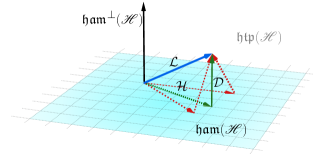
Figure 1: Decomposition of the generator $\mathcal{L}$ into some Hamiltonian contribution $\mathcal{H}\in\mathfrak{ham}(\mathscr{H})$ and a dissipator $\mathcal{D}$. The dissipator part $\mathcal{D}$ can generically admit a component on $\mathfrak{ham}(\mathscr{H})$; the unique dissipator given by the orthogonal decomposition (11), defined through the scalar product (10), is the one with minimal associated norm $||\mathcal{D}||$.

We can now give a simple geometric picture of the principle of minimal dissipation (see Fig. 1). To this end, let us define the subspace $\mathfrak{ham}(\mathscr{H})$ of $\mathfrak{htp}(\mathscr{H})$ which is formed by all Hamiltonian superoperators of the form of $\mathcal{H}_{t}$ (see Eq. (4)), i.e. by all superoperators $\mathcal{H}\in\mathfrak{htp}(\mathscr{H})$ for which there exists a Hermitian operator $H$ such that $\mathcal{H}[A]=-\mathrm{i}[H,A]\;\;\forall A\in\mathcal{B}(\mathscr{H})$. Given a superoperator $\mathcal{L}_{t}$ one defines the Hamiltonian part $\mathcal{H}_{t}$ as the orthogonal projection of $\mathcal{L}_{t}$ onto the subspace $\mathfrak{ham}(\mathscr{H})$ defined by the scalar product (10). Denoting the corresponding projection by $\Pi$ one thus has

$$\mathcal{H}_{t}=\Pi(\mathcal{L}_{t}),\quad\mathcal{D}_{t}=\mathcal{L}_{t}-\Pi(\mathcal{L}_{t}).$$ (11)

Note that this splitting corresponds to the orthogonal decomposition $\mathfrak{htp}(\mathscr{H})=\mathfrak{ham}(\mathscr{H})\oplus\mathfrak{ham}^{\perp}(\mathscr{H})$ with respect to the scalar product associated to the norm.

It is clear that the above construction yields unique expressions for the Hamiltonian part and the dissipator of the master equation. Moreover, among all possible decompositions of the generator into a Hamiltonian part and a dissipator, the one given by Eq. (11) has the least norm of the dissipator. This is why we call this the principle of minimal dissipation: it states that we uniquely define the dissipator of the master equation, which will be associated with heat exchange, by making its average effect on physical states as small as possible, shifting as much as possible into the Hamiltonian contribution. In view of this interpretation the choice of the particular norm (9) is physically reasonable because it is a democratic norm which measures the size of superoperators by giving equal weight to all pure states. Most remarkable, it has been demonstrated in Ref. Sorce and Hayden (2022) that a minimal norm of the dissipator exactly corresponds to taking traceless Lindblad operators (for an alternative proof see Appendix B). Thus, to satisfy the principle of minimal dissipation in practice one only has to ensure that the Lindblad operators are traceless for all times, which can always be achieved by a suitable transformation of the form (6). We note that the Lindblad operators are often already traceless when the master equation is derived perturbatively from a microscopic model. This is the case, for example, for the standard weak-coupling semigroup master equation in Lindblad form Breuer and Petruccione (2002) whose Lindblad operators are eigenoperators of the system Hamiltonian $H_{S}$ and, hence, are automatically traceless.

IV First and second law of thermodynamics

Fixing the unique splitting of the generator into $\mathcal{H}_{t}$ and $\mathcal{D}_{t}$ according to the principle of minimal dissipation allows us to identify the associated Hamiltonian $K_{S}(t)$ as an effective Hamiltonian for the system, that encompasses the collective effects of the bath onto it. The variation of internal energy of the system can be then defined as $\Delta U_{S}(t)=\mathrm{Tr}\{K_{S}(t)\rho_{S}(t)\}-\mathrm{Tr}\{K_{S}(0)\rho_{S}(0)\}$ such that the first law arises naturally as

$$\Delta U_{S}(t)=\delta W_{S}(t)+\delta Q_{S}(t)$$ (12)

by defining work and heat contributions as

$$\delta W_{S}(t) = \int_{0}^{t}\mathrm{d}\tau\,\mathrm{Tr}\big{\{}\dot{K}_{S}(\tau)\rho_{S}(\tau)\big{\}},$$ (13)

$$\delta Q_{S}(t) = \int_{0}^{t}\mathrm{d}\tau\,\mathrm{Tr}\big{\{}K_{S}(\tau)\dot{\rho}_{S}(\tau)\big{\}}.$$ (14)

Here, the heat contribution turns out to be only due to the dissipative part of the evolution of the density matrix since the above can be written as

$$\delta Q_{S}(t)=\int_{0}^{t}\mathrm{d}\tau\,\mathrm{Tr}\big{\{}K_{S}(\tau)\mathcal{D}_{\tau}[\rho_{S}(\tau)]\big{\}}.$$ (15)

It is worth mentioning that it is possible for the effective Hamiltonian $K_{S}$ to be time dependent even if the original system Hamiltonian $H_{S}$ is not. For instance, this is the case for the example discussed in Sec. V. Through this our approach admits the appearance of effective work done on the system as a result of the interaction with the bath. This feature is shared with other approaches (see, e.g., Weimer et al. (2008); Teifel and Mahler (2011); Alipour et al. (2016)). Note that this does not contradict the idea that a change in internal energy of a closed system should be identified with work. It is a well-known fact, which holds of course also in our formalism, that a change in the internal energy of the total system can only be due to explicit time dependencies of the total system Hamiltonian. However, contrary to what is assumed in many alternative approaches Rivas (2020); Strasberg and Esposito (2020a); Talkner and Hänggi (2020a), this does not imply that the change in internal energy of the total system should be identified with work done on the open system only. As emerges from our formalism the environment can perform work on the open system, even when the total system Hamiltonian is time independent and, hence, the internal energy of the total closed system does not change: In such a case there is an exchange of energy between the open system and its environment which manifests itself in the time dependence of the effective system Hamiltonian $K_{S}(t)$ and must be interpreted as mechanical work.

As a result of the above definition of heat exchange, the entropy production is defined as

$$\Sigma_{S}(t)=\Delta S_{S}(t)-\beta\delta Q_{S}(t)\;,$$ (16)

with $\Delta S_{S}(t)=S(\rho_{S}(t))-S(\rho_{S}(0))$ the change of the von Neumann entropy of the reduced system and $\beta=1/\mathrm{k_{B}}T$ the inverse temperature of the bath. For simplicity we assume here that the environment is sufficiently large such that its temperature can be regarded as effectively constant as has been discussed recently Strasberg et al. (2021). An alternative expression for the entropy production is given by

$$\Sigma_{S}(t) = S(\rho_{S}(0)||\rho_{S}^{\mathrm{G}}(0))-S(\rho_{S}(t)||\rho_{S}^{\mathrm{G}}(t))$$ (17)

$$-\int_{0}^{t}\mathrm{d}\tau\,\mathrm{Tr}\big{\{}\rho_{S}(\tau)\partial_{\tau}\ln\rho_{S}^{\mathrm{G}}(\tau)\big{\}},$$

with $S(\rho_{A}||\rho_{B})$ the relative entropy of the states $\rho_{A}$ and $\rho_{B}$, and where one utilizes the instantaneous Gibbs states associated to the effective Hamiltonian $K_{S}(t)$, namely $\rho_{S}^{\text{G}}(t)=e^{-\beta K_{S}(t)}/Z_{S}(t)$. It is important to note that the structure of expression (17) for the entropy production is the same as the one derived in Ref. Deffner and Lutz (2011). The crucial difference is, however, that in our expression the effective Hamiltonian $K_{S}(t)$ appears, while in Deffner and Lutz (2011) this Hamiltonian is replaced by the microscopic system Hamiltonian $H_{S}(t)$ (see Eq. (1)). As a consequence of the fact that $K_{S}(t)$ contains the effective influence of the bath on the open system, our expression is valid also outside of the weak-coupling regime. As expected, in the limit of vanishing coupling our expression (17) for the entropy production reduces for arbitrary driving to the one obtained in Deffner and Lutz (2011). To see this we recall that the master equation (2) and, in particular, the effective Hamiltonian $K_{S}(t)$ can be derived from the total Hamiltonian (1) by means of the time-convolutionless projection operator technique Shibata et al. (1977); Chaturvedi and Shibata (1979); Breuer and Petruccione (2002). This technique leads to a perturbation expansion for the effective Hamiltonian $K_{S}(t,\lambda)$ in powers of the size $\lambda$ of the system-environment interaction which takes the following form,

$$K_{S}(t,\lambda)=H_{S}(t)+\lambda^{2}G_{S}(t)+{\mathcal{O}}(\lambda^{4}).$$ (18)

This shows that in the limit $\lambda\to 0$ the effective Hamiltonian reduces to the bare Hamiltonian $H_{S}(t)$ of the open system, appearing in the microscopic Hamiltonian (1) of the total system. Consequently, in this limit also (17) reduces to the expression derived in Deffner and Lutz (2011). Moreover, if $H_{S}$ is time independent and the open system dynamics is described by a quantum Markovian semigroup we recover the earlier results of Ref. Spohn (1978).

Taking the time derivative of Eq. (17) we obtain the entropy production rate

$$\sigma_{S}(t) \equiv \dot{\Sigma}_{S}(t)=-\frac{\mathrm{d}}{\mathrm{d}\tau}\Bigg{|}_{\tau=0}S(\rho_{S}(t+\tau)||\rho_{S}^{\mathrm{G}}(t))$$ (19)

$$= -\mathrm{Tr}\big{\{}\mathcal{D}_{t}[\rho_{S}(t)]\big{(}\ln\rho_{S}(t)-\ln\rho_{S}^{\mathrm{G}}(t)\big{)}\big{\}}\;.$$

The expression given in the first line relates the entropy production rate to the derivative of the relative entropy, where the notation indicates that $\rho_{S}^{\mathrm{G}}$ should be regarded as a constant under the time derivative, while the second line connects it directly to the dissipator of the master equation. Let us assume that the Gibbs state $\rho_{S}^{\text{G}}(t)$ represents an instantaneous fixed point of the evolution Strasberg and Esposito (2019); Altaner (2017), namely that there is no instantaneous dissipation for this state: $\mathcal{L}_{t}[\rho_{S}^{\text{G}}(t)]=\mathcal{D}_{t}[\rho_{S}^{\text{G}}(t)]=0$. Under this condition one can show that the entropy production rate is positive if the dynamical map $\Phi_{t}$ is P-divisible Breuer et al. (2016), i.e., one has

$$\sigma_{S}(t)\geq 0\;,$$ (20)

which corresponds to the second law. Note that we associate here the second law with the positivity of the entropy production rate, which implies an increase of entropy over all time intervals (see, e.g., Ref. Strasberg et al. (2017)). To prove (20) one uses the fact that the relative entropy decreases under the application of a positive trace preserving map to both of its arguments Müller-Hermes and Reeb (2017).

Finally, it might be interesting to discuss how possible violations of the second law are related to the non-Markovianity of the underlying dynamics, i.e. to the presence of quantum memory effects Breuer et al. (2016). To this end, we employ the definition for quantum non-Markovianity based on the information flow between the open system and its environment Breuer et al. (2009, 2016). The key idea is to characterize Markovian behavior in the quantum regime through a continuous loss of information, i.e. by a flow of information from the open system to the environment. Correspondingly, quantum memory effects feature a flow of information from the environment back to the system. Quantifying the information content by means of the distinguishability of quantum states as measured by the Hellstrom matrix, one can show that Markovianity of quantum processes in open systems is equivalent to P-divisibility of the corresponding dynamical map Chruściński et al. (2011); Wißmann et al. (2015). Recall that P-divisibility means that the propagator $\Phi_{t,s}$ which maps the open system states at time $s$ to the open system states at time $t$ is a positive map for all $t\geq s\geq 0$. One the other hand, we have just seen that under the condition that the Gibbs state is an instantaneous fixed point P-divisibility implies positivity of the entropy production rate. We conclude that in order for Eq. (20) to be violated the process must break P-divisibility and, hence, must be non-Markovian. Thus, we see that non-Markovianity, i.e. memory effects are a necessary condition for violations of the second law.

V Example

To illustrate our theory we briefly discuss the model of a two-state atom, regarded as the open system, coupled to a single harmonic oscillator mode, which is also known as Jaynes-Cummings model. The total Hamiltonian is time independent and of the form of Eq. (1). The time independent system Hamiltonian is given by

$$H_{S}=\omega_{0}\sigma_{+}\sigma_{-},$$ (21)

where $\omega_{0}$ denotes the transition frequency of the two-state system with excited state $|1\rangle$ and ground state $|0\rangle$, while $\sigma_{\pm}$ are the usual Pauli raising and lowering operators. The environmental Hamiltonian is given by $H_{E}=\omega b^{\dagger}b$, where $\omega$ is the eigenfrequency of the harmonic oscillator and $b$, $b^{\dagger}$ denote the annihilation and creation operator, respectively. Finally, the time independent interaction Hamiltonian is taken to be of the Jaynes-Cummings form

$$H_{I}=g(\sigma_{+}b+\sigma_{-}b^{\dagger}),$$ (22)

where $g$ is a coupling constant.

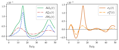
Figure 2: Left: Change of internal energy $\Delta U_{S}$, work $\delta W_{S}$ and heat $\delta Q_{S}$ as a function of time for the Jaynes-Cummings model with effective system Hamiltonian (23). Right: Comparison between the entropy production rate $\sigma_{S}$ according to Eq. (19) and its weak-coupling version $\sigma_{S}^{\mathrm{w}}$ for the same model. Parameters: $g=0.1\omega_{0}$, $\omega=0.9\omega_{0}$, $\mathrm{k_{B}}T=\omega_{0}$, $\rho_{S}^{11}(0)=0.25$ and $\rho_{S}^{10}(0)=0$.

Assuming the oscillator to be initially in a thermal equilibrium state at a certain temperature $T$ one can derive an exact master equation for the dynamics of the two-state system Smirne and Vacchini (2010) which is of the form given by Eqs. (2)-(5). The dissipator of the master equation can be written in terms of the three traceless and time-independent Lindblad operators $L_{1}=\sigma_{-}$, $L_{2}=\sigma_{+}$ and $L_{3}=\sigma_{z}$ with corresponding time dependent rates $\gamma_{k}(t)$, $k=1,2,3$. The effective system Hamiltonian takes the form

$$K_{S}(t)=\big{[}\omega_{0}+\Delta\omega(t)\big{]}\sigma_{+}\sigma_{-}.$$ (23)

Comparing Eqs. (21) and (23) we see that the interaction of the system with the environmental mode leads to a time dependent frequency shift $\Delta\omega(t)$, which in general depends on the system-environment coupling $g$ and on temperature $T$. Further details and the expression for the frequency renormalization $\Delta\omega(t)$ may be found in Smirne and Vacchini (2010). Here, we plot the results for the decomposition (12) of the change of internal energy into work (13) and heat (14), and the comparison between the entropy production rate (19) and its weak-coupling counterpart Spohn (1978), see Fig. 2. We observe that there is a significant contribution of work to the change of internal energy, although the total Hamiltonian is time independent, which is due to the time dependence of the effective system Hamiltonian (23). We also see that the magnitude of the entropy production rate is substantially larger than the one given by the weak-coupling expression.

VI Conclusions and remarks

We have formulated a general nonperturbative approach to the quantum thermodynamics of open systems based on the exact time-convolutionless master equation of the open system and on the principle of minimal dissipation, which allows to develop unique expressions for work, heat and entropy production. As we have demonstrated the principle of minimal dissipation leads to a unique effective system Hamiltonian $K_{S}(t)$ which generates the coherent part of the open system dynamics and defines the internal energy of the system as it results from the cooperative effect of system and environment. As we have seen the effective system Hamiltonian $K_{S}(t)$ can be time dependent even though the total microscopic system Hamiltonian $H$ in Eq. (1) is time independent. Thus, for non-Markovian dynamics the environment can do work on the open system, or extract work from it, as is illustrated in the example of Sec. V. In our opinion this is an important consequence of our approach which could lead to interesting applications. We further emphasize that our strategy of constructing an effective open system Hamiltonian can also be applied to approximate time-local master equations, such as the quantum optical, the Brownian motion, the Redfield, or, more generally, the TCL master equations in any finite order of perturbation theory Breuer and Petruccione (2002).

An important feature of our theory is the fact that it only refers to open system variables, i.e., only degrees of freedom of the open system enter the definitions of thermodynamic quantities. Thus, in contrast to other approaches (see, e.g., Ref. Esposito et al. (2010)) the application of our method does not require the control or measurement of environmental variables. As a consequence we were able to establish under certain conditions a connection of our formulation of the second law with the concept of quantum non-Markovianity based on the information flow between system and environment. This connection yields a natural information theoretic interpretation because it implies that a backflow of information from the environment to the open system is a necessary condition for violations of the second law.

We finally remark that the pillars of our approach, namely the TCL master equation and the principle of minimal dissipation, have been formally proven only for open systems with finite-dimensional Hilbert spaces. The generalization of the method developed here to the case of (bounded or even unbounded) generators on an infinite-dimensional Hilbert space represents a challenging mathematical project, but is extremely interesting and relevant from a physical point of view.

Appendix A Invariance of the generator

The generator $\mathcal{L}=-\text{i}[K,\cdot]+\mathcal{D}$ is invariant under the addition of a time dependent constant to the Lindblad operators, and a consequent additional term to the Hamiltonian $K$, although this is not the most general invariance. In fact, it is also permitted to modify the dissipator by absorbing the rate amplitudes into the Lindblad operators, or to mix them through a generalized unitary transformation which preserves the sign of the rates. To see this, let us first rewrite the dissipator at a fixed time $t$, in particular by grouping the Lindblad operators associated to positive rates to lower indices, such that we can express it in the following way:

$$\mathcal{D}=\sum_{ij}J_{ij}\sqrt{|\gamma_{i}||\gamma_{j}|}\left[L_{i}\rho L_{j}^{\dagger}-\frac{1}{2}\{L_{i}^{\dagger}L_{j},\rho\}\right]\;,$$ (24)

where we defined the matrix describing the sign of the rates

$$J=\begin{bmatrix}\mathbb{I}_{p}&0\\ 0&-\mathbb{I}_{q}\end{bmatrix}\;,$$ (25)

and where $p$ ($q$) is taken to be the number of positive (negative) rates. Note that this exact division into positive and negative rates may depend on time; still, this description is applicable at any fixed time $t$. Defining the bilinear form

$$\left(\vec{v},\vec{w}\right):=\vec{v}\cdot J\vec{w}$$ (26)

and absorbing the rates $\sqrt{|\gamma_{i}|}$ into the definition of the Lindblad operators, we can formally rewrite the dissipator as

$$\mathcal{D}=(\vec{L},\rho\vec{L}^{\dagger})-\frac{1}{2}\{(\vec{L}^{\dagger},\vec{L}),\rho\}\;,$$ (27)

where we have defined $\vec{L}$ as the vector of all $N^{2}-1$ Lindblad operators.

It is straightforward to prove that the generator $\mathcal{L}$ is at each time invariant under the transformation

$$\vec{L} \longrightarrow\Upsilon\vec{L}+\vec{\alpha}$$ (28)

$$K \longrightarrow K+\frac{1}{2\text{i}}\left[(\vec{\alpha}^{*},\Upsilon\vec{L})-(\vec{\alpha},\Upsilon^{*}\vec{L}^{\dagger})\right]+\beta$$ (29)

given by the parameters $(\vec{\alpha}\in\mathbb{C}^{N^{2}-1},\Upsilon\in\mathrm{U}(p,q),\beta\in\mathbb{R})$, where $U(p,q)$ is the indefinite (sometimes also called generalized) unitary group of matrices satisfying

$$\Upsilon^{\dagger}J\Upsilon=J\;.$$ (30)

The transformations of the generator obey the following group property

$$(\vec{\alpha}^{\prime},\Upsilon^{\prime},\beta^{\prime})(\vec{\alpha},\Upsilon,\beta)=(\vec{\alpha}^{\prime}+\Upsilon^{\prime}\vec{\alpha},\Upsilon^{\prime}\Upsilon,\beta^{\prime}+\beta+\text{Im}(\vec{\alpha}^{\prime},\Upsilon^{\prime}\vec{\alpha}))\;.$$ (31)

When the dynamics happens to be CP-divisible, namely when $J\equiv\mathbb{I}$, this invariance reduces to the one of a generator of a Lindblad master equation Breuer and Petruccione (2002) where $\Upsilon$ is a unitary transformation, albeit still with time dependent parameters.

Appendix B Derivation of the dissipator of minimal norm

The space of generators of quantum master equations can be orthogonally decomposed into

$$\mathfrak{htp}(\mathscr{H})=\mathfrak{ham}(\mathscr{H})\oplus\mathfrak{ham}^{\perp}(\mathscr{H})\;,$$ (32)

such that at fixed time $t$, any generator $\mathcal{L}$ can be written as $\mathcal{L}=\mathcal{H}+\mathcal{D}$, with $\mathcal{H}\in\mathfrak{ham}(\mathscr{H})$. To find the unique decomposition such that $\mathcal{D}$ is in the orthogonal subspace $\mathfrak{ham}^{\perp}(\mathscr{H})$, we project the generator onto $\mathfrak{ham}(\mathscr{H})$:

$$\mathcal{H}=\Pi(\mathcal{L})=\sum_{j}\mathcal{H}_{j}\langle\mathcal{H}_{j},\mathcal{L}\rangle\;,$$ (33)

with $\{\mathcal{H}_{j}\}_{j=1}^{N^{2}-1}$ an orthonormal basis of $\mathfrak{ham}(\mathscr{H})$, through the scalar product on $\mathfrak{htp}(\mathscr{H})$

$$\langle\mathcal{X}_{1},\mathcal{X}_{2}\rangle=\overline{\bra{\psi}\overline{\mathcal{X}_{1}[\ket{\phi}\bra{\phi}]\mathcal{X}_{2}[\ket{\phi}\bra{\phi}]}\ket{\psi}}\;.$$ (34)

Here, $\ket{\phi}$ and $\ket{\psi}$ are random Haar states

$$\ket{\phi}=U\ket{\phi_{0}}\;,$$ (35)

with $\ket{\phi_{0}}$ a fixed normalized state and $U\in\mathrm{U}(N)$ a random unitary, while $\overline{\bra{\phi}X\ket{\phi}}$ denotes the Haar average of an operator $X$ over $\ket{\phi}$.

As a recurring tool, let us notice that, as a consequence of Schur’s Lemma and the invariance of the Haar measure under multiplication with unitaries, it holds for any operator $X\in\mathcal{B}(\mathscr{H})$ that

$$X^{\prime}:=\int\mathrm{d}\mu(U)U^{\dagger}XU=c\cdot\mathbb{I}\;,\quad c\in\mathbb{C}\;,$$ (36)

so that, by taking the trace of the above, one finds

$$\int\mathrm{d}\mu(U)U^{\dagger}XU=\frac{\mathrm{Tr}\{X\}}{N}\mathbb{I}\;.$$ (37)

Naturally this entails that the Haar average of $X$ is simply given by

$$\overline{\bra{\psi}X\ket{\psi}}=\frac{\mathrm{Tr}X}{N}\;,$$ (38)

and that the norm associated to the scalar product (34) reads:

$$||\mathcal{L}||^{2}=\frac{1}{N}\mathrm{Tr}\left\{\overline{\mathcal{L}\left[\ket{\phi}\bra{\phi}\right]^{2}}\right\}\;.$$ (39)

To find the expression for the Hamiltonian $K$ generating $\mathcal{H}=-\text{i}[K,\cdot]$, we exploit the fact that $\mathfrak{ham}(\mathscr{H})$ is isomorphic to the space of traceless hermitian operators $\mathrm{Herm_{tl}}(\mathscr{H})=\{H\in\mathcal{B}(\mathscr{H})|H^{\dagger}=H,\;\mathrm{Tr}\{H\}=0\}$. With this we can exploit the connection between a basis of superoperators in $\mathfrak{ham}(\mathscr{H})$ and one of operators in $\mathrm{Herm_{tl}}(\mathscr{H})$ found in the following Lemma.

Lemma 1.

Each element of an orthonormal basis $\{\mathcal{H}_{j}\}_{j=1}^{N^{2}-1}$ of $\mathfrak{ham}(\mathscr{H})$ with respect to the scalar product (34) is such that

$$\mathcal{H}_{j}=-\mathrm{i}[H_{j},\cdot]\;,$$ (40)

where $\{H_{j}\}_{j=1}^{N^{2}-1}$ is an orthogonal basis with respect to the Hilbert-Schmidt product on $\mathrm{Herm_{tl}}(\mathscr{H})$ satisfying

$$\mathrm{Tr}\{H_{i}H_{j}\}=\frac{N(N+1)}{2}\delta_{ij}\;.$$ (41)

Proof.

From (38) and the normalization of $\ket{\phi}$, one has that

$$\langle\mathcal{H}_{i},\mathcal{H}_{j}\rangle= \frac{1}{N}\mathrm{Tr}\left\{\overline{\mathcal{H}_{i}[\ket{\phi}\bra{\phi}]\mathcal{H}_{j}[\ket{\phi}\bra{\phi}]}\right\}$$

$$= \underbrace{\frac{1}{N}\mathrm{Tr}\left\{\{H_{i},H_{j}\}\overline{\ket{\phi}\bra{\phi}}\right\}}_{(a)}$$

$$\quad\quad\underbrace{-\frac{1}{N}\mathrm{Tr}\left\{2H_{i}\overline{\ket{\phi}\bra{\phi}H_{j}\ket{\phi}\bra{\phi}}\right\}}_{(b)}\;.$$ (42)

The second moment term $(a)$ is simply given by $\frac{2}{{N^{2}}}\mathrm{Tr}\left\{H_{i}H_{j}\right\}$ through identity (37), while the fourth moment Haar integral found in $(b)$ is less straightforward to calculate. One can make use of the following general formula (see, e.g., Ref. Gessner and Breuer (2013)):

$$\int\mathrm{d}\mu(U) UX_{1}U^{\dagger}X_{2}UX_{3}U^{\dagger}=$$

$$= {N\mathrm{Tr}\{X_{3}X_{1}\}-\mathrm{Tr}\{X_{1}\}\mathrm{Tr}\{X_{3}\}\over N(N^{2}-1)}\left(\mathrm{Tr}\{X_{2}\}\right)\mathbb{I}$$

$$+{N\mathrm{Tr}\{X_{1}\}\mathrm{Tr}\{X_{3}\}-\mathrm{Tr}\{X_{3}X_{1}\}\over N(N^{2}-1)}X_{2}\;,$$ (43)

and the tracelessness of $H_{j}$ to find that $(b)$ reads $-{2\over{N^{2}(N+1)}}\mathrm{Tr}\left\{H_{i}H_{j}\right\}$. Imposing the orthogonality of the basis of $\mathrm{Herm_{tl}}(\mathscr{H})$ (41), one recovers

$$\langle\mathcal{H}_{i},\mathcal{H}_{j}\rangle=\delta_{ij}\;.$$ (44)

∎

It is then straightforward that the Hamiltonian operator associated to $\mathcal{H}$ is given by

$$K=\sum_{j}H_{j}\langle\mathcal{H}_{j},\mathcal{L}\rangle\;.$$ (45)

To find the expression for the coefficients $\langle\mathcal{H}_{j},\mathcal{L}\rangle$, we make use of the pseudo-Kraus representation for the generator, which states that any Hermiticity preserving map can be written as $\mathcal{L}[\rho]=\sum_{k}\gamma_{k}E_{k}\rho E_{k}^{\dagger}$ with some operators $E_{k}$ and real (not necessarily positive) coefficients $\gamma_{k}$ Choi (1975). Employing (38) we then find

$$\langle\mathcal{H}_{j},\mathcal{L}\rangle =-{\text{i}\over N}\sum_{k}\gamma_{k}\mathrm{Tr}\Big{\{} \overline{[H_{j},\ket{\phi}\bra{\phi}]E_{k}\ket{\phi}\bra{\phi}E_{k}^{\dagger}}\Big{\}}$$ (46)

$$=-{\text{i}\over N}\sum_{k}\gamma_{k}\mathrm{Tr}\Big{\{} H_{j}\overline{\ket{\phi}\bra{\phi}E_{k}\ket{\phi}\bra{\phi}}E_{k}^{\dagger}$$

$$\quad-H_{j}E_{k}\overline{\ket{\phi}\bra{\phi}E_{k}^{\dagger}\ket{\phi}\bra{\phi}}\Big{\}}$$

$$=-{1\over N^{2}(N+1)}\sum_{k} \gamma_{k}\mathrm{Tr}\{H_{j}Y_{k}\}\;,$$

where we used again expression (1) for the fourth moment Haar integral and have defined the operators

$$Y_{k}=\text{i}(\mathrm{Tr}\{E_{k}\}E_{k}^{\dagger}-\mathrm{Tr}\{E_{k}^{\dagger}\}E_{k})\;.$$ (47)

From the completeness of the basis $H_{j}$ and Lemma 1, and since each operator $Y_{k}$ is in $\mathrm{Herm_{tl}}(\mathscr{H})$, one has

$$\sum_{j}H_{j}\mathrm{Tr}\{H_{j}Y_{k}\}={N(N+1)\over 2}Y_{k}\;,$$ (48)

so that the expression for the Hamiltonian generating the projection of $\mathcal{L}$ onto $\mathfrak{ham}(\mathscr{H})$ reads

$$K=-{\text{i}\over 2N}\sum_{k}\gamma_{k}\left[\mathrm{Tr}\{E_{k}\}E_{k}^{\dagger}-\mathrm{Tr}\{E_{k}^{\dagger}\}E_{k}\right]\;.$$ (49)

Then, the physical dissipator will be given by the remaining contribution and will have minimal norm:

$$\mathcal{D}[\rho]= \mathcal{L}[\rho]-\Pi(\mathcal{L}[\rho])$$

$$= \sum_{k}\gamma_{k}E_{k}\rho E_{k}^{\dagger}$$

$$+{1\over 2N}\sum_{k}\gamma_{k}\left[\mathrm{Tr}\{E_{k}\}E_{k}^{\dagger}-\mathrm{Tr}\{E_{k}^{\dagger}\}E_{k},\rho\right]\;.$$ (50)

From the requirement that $\mathcal{L}\in\mathfrak{htp}(\mathscr{H})$, which means that $\mathcal{L}$ is not only Hermiticity but also trace preserving, one gets the additional condition on the set of pseudo-Kraus operators:

$$\sum_{k}\gamma_{k}E_{k}^{\dagger}E_{k}=0\;.$$ (51)

With this, one can rewrite the dissipator in the desired form

$$\mathcal{D}[\rho]=\sum_{k}\gamma_{k}\left[L_{k}\rho L_{k}^{\dagger}-{1\over 2}\{L_{k}^{\dagger}L_{k},\rho\}\right]\;,$$ (52)

where the Lindblad operators are found to be traceless:

$$L_{k}=E_{k}-{\mathrm{Tr}\{E_{k}\}\over N}\mathbb{I}\;.$$ (53)

Given a generator, fixing the Lindblad operators to be traceless at all times also fixes the expression for the Hamiltonian $K$ (up to a time-dependent constant). Absorption of the rates $\gamma_{k}$ or a mixing of the Lindblad operators are still allowed, but leave the dissipator and the Hamiltonian separately invariant. Therefore, the dissipator which has minimal norm (39) is unique, and is written in terms of traceless Lindblad operators $L_{k}$.

References

- Gemmer et al. (2004) J. Gemmer, M. Michel, and G. Mahler, Quantum Thermodynamics (Springer, Berlin, 2004).
- Schaller (2014) G. Schaller, Open Quantum Systems Far from Equilibrium (Springer, Cham, Switzerland, 2014).
- Binder et al. (2018) F. Binder, L. A. Correa, C. Gogolin, J. Anders, and G. Adesso, Thermodynamics in the Quantum Regime (Springer, Cham, Switzerland, 2018).
- Deffner and Campbell (2019) S. Deffner and S. Campbell, Quantum Thermodynamics: An introduction to the thermodynamics of quantum information, 2053-2571 (Morgan & Claypool Publishers, 2019).
- Landi and Paternostro (2021) G. T. Landi and M. Paternostro, Rev. Mod. Phys. 93, 035008 (2021).
- Breuer and Petruccione (2002) H.-P. Breuer and F. Petruccione, The Theory of Open Quantum Systems (Oxford University Press, Oxford, 2002).
- Weimer et al. (2008) H. Weimer, M. J. Henrich, F. Rempp, H. Schröder, and G. Mahler, EPL (Europhysics Letters) 83, 30008 (2008).
- Esposito et al. (2010) M. Esposito, K. Lindenberg, and C. V. den Broeck, New Journal of Physics 12, 013013 (2010).
- Teifel and Mahler (2011) J. Teifel and G. Mahler, Phys. Rev. E 83, 041131 (2011).
- Alipour et al. (2016) S. Alipour, F. Benatti, F. Bakhshinezhad, M. Afsary, S. Marcantoni, and A. T. Rezakhani, Scientific Reports 6, 35568 (2016).
- Strasberg et al. (2017) P. Strasberg, G. Schaller, T. Brandes, and M. Esposito, Phys. Rev. X 7, 021003 (2017).
- Popovic et al. (2018) M. Popovic, B. Vacchini, and S. Campbell, Phys. Rev. A 98, 012130 (2018).
- Strasberg and Esposito (2019) P. Strasberg and M. Esposito, Phys. Rev. E 99, 012120 (2019).
- Rivas (2020) A. Rivas, Phys. Rev. Lett. 124, 160601 (2020).
- Alipour et al. (2021) S. Alipour, A. T. Rezakhani, A. Chenu, A. del Campo, and T. Ala-Nissila, “Entropy-based formulation of thermodynamics in arbitrary quantum evolution,” (2021), arXiv:1912.01939 [quant-ph] .
- Seifert (2016) U. Seifert, Phys. Rev. Lett. 116, 020601 (2016).
- Campisi et al. (2009) M. Campisi, P. Talkner, and P. Hänggi, Journal of Physics A: Mathematical and Theoretical 42, 392002 (2009).
- Talkner and Hänggi (2016) P. Talkner and P. Hänggi, Phys. Rev. E 94, 022143 (2016).
- Talkner and Hänggi (2020a) P. Talkner and P. Hänggi, Rev. Mod. Phys. 92, 041002 (2020a).
- Strasberg and Esposito (2020a) P. Strasberg and M. Esposito, Phys. Rev. E 101, 050101 (2020a).
- Strasberg and Esposito (2020b) P. Strasberg and M. Esposito, Phys. Rev. E 102, 066102 (2020b).
- Talkner and Hänggi (2020b) P. Talkner and P. Hänggi, Phys. Rev. E 102, 066101 (2020b).
- Spohn (1978) H. Spohn, Journal of Mathematical Physics 19, 1227 (1978).
- Spohn and Lebowitz (1978) H. Spohn and J. L. Lebowitz, “Irreversible thermodynamics for quantum systems weakly coupled to thermal reservoirs,” in Advances in Chemical Physics (John Wiley & Sons, Ltd, 1978) pp. 109–142.
- Kosloff (2013) R. Kosloff, Entropy 15, 2100 (2013).
- Breuer et al. (2016) H.-P. Breuer, E.-M. Laine, J. Piilo, and B. Vacchini, Rev. Mod. Phys. 88, 021002 (2016).
- de Vega and Alonso (2017) I. de Vega and D. Alonso, Rev. Mod. Phys. 89, 015001 (2017).
- Sorce and Hayden (2022) J. Sorce and P. M. Hayden, Journal of Physics A: Mathematical and Theoretical (2022), 10.1088/1751-8121/ac65c2.
- Marcantoni et al. (2017) S. Marcantoni, S. Alipour, F. Benatti, R. Floreanini, and A. T. Rezakhani, Sci. Rep. 7, 12447 (2017).
- Stelmachovic and Buzek (2001) P. Stelmachovic and V. Buzek, Phys. Rev. A 64, 062106 (2001).
- Breuer (2012) H.-P. Breuer, J. Phys. B 45, 154001 (2012).
- Hall et al. (2014) M. J. W. Hall, J. D. Cresser, L. Li, and E. Andersson, Phys. Rev. A 89, 042120 (2014).
- Gorini et al. (1976) V. Gorini, A. Kossakowski, and E. C. G. Sudarshan, J. Math. Phys. 17, 821 (1976).
- Nakajima (1958) S. Nakajima, Progr. Theor. Phys. 20, 948 (1958).
- Zwanzig (1960) R. Zwanzig, J. Chem. Phys. 33, 1338 (1960).
- Shibata et al. (1977) F. Shibata, Y. Takahashi, and N. Hashitsume, J. Stat. Phys. 17, 171 (1977).
- Chaturvedi and Shibata (1979) S. Chaturvedi and F. Shibata, Z. Phys. B 35, 297 (1979).
- Lindblad (1976) G. Lindblad, Communications in Mathematical Physics 48, 119 (1976).
- Hu et al. (1992) B. L. Hu, J. P. Paz, and Y. Zhang, Phys. Rev. D 45, 2843 (1992).
- Ferialdi (2016) L. Ferialdi, Phys. Rev. Lett. 116, 120402 (2016).
- Zhang et al. (2012) W.-M. Zhang, P.-Y. Lo, H.-N. Xiong, M. W.-Y. Tu, and F. Nori, Phys. Rev. Lett. 109, 170402 (2012).
- Huang and Zhang (2020) W.-M. Huang and W.-M. Zhang, “Strong coupling quantum thermodynamics with renormalized hamiltonian and temperature,” (2020), arXiv:2010.01828 [quant-ph] .
- Breuer et al. (1999) H.-P. Breuer, B. Kappler, and F. Petruccione, Phys. Rev. A 59, 1633 (1999).
- Ban et al. (2010) M. Ban, S. Kitajima, and F. Shibata, Phys. Lett. A 374, 2324 (2010).
- Doll et al. (2008) R. Doll, D. Zueco, M. Wubs, S. Kohler, and P. Hänggi, Chemical Physics 347, 243 (2008).
- Bhattacharya et al. (2017) S. Bhattacharya, A. Misra, C. Mukhopadhyay, and A. K. Pati, Phys. Rev. A 95, 012122 (2017).
- Note (1) There is an additional invariance induced by an indefinite unitary transformation of the set of Lindblad operators; since this is not particularly relevant for the topic of this paper, we report it for completeness in Appendix A.
- Collins and Śniady (2006) B. Collins and P. Śniady, Commun. Math. Phys. 264, 773 (2006).
- Strasberg et al. (2021) P. Strasberg, M. G. Díaz, and A. Riera-Campeny, Phys. Rev. E 104, L022103 (2021).
- Deffner and Lutz (2011) S. Deffner and E. Lutz, Phys. Rev. Lett. 107, 140404 (2011).
- Altaner (2017) B. Altaner, Journal of Physics A: Mathematical and Theoretical 50, 454001 (2017).
- Müller-Hermes and Reeb (2017) A. Müller-Hermes and D. Reeb, Ann. Henri Poincaré 18, 1777 (2017).
- Breuer et al. (2009) H.-P. Breuer, E.-M. Laine, and J. Piilo, Phys. Rev. Lett. 103, 210401 (2009).
- Chruściński et al. (2011) D. Chruściński, A. Kossakowski, and A. Rivas, Phys. Rev. A 83, 052128 (2011).
- Wißmann et al. (2015) S. Wißmann, B. Vacchini, and H.-P. Breuer, Phys. Rev. A 92, 042108 (2015).
- Smirne and Vacchini (2010) A. Smirne and B. Vacchini, Phys. Rev. A 82, 022110 (2010).
- Gessner and Breuer (2013) M. Gessner and H.-P. Breuer, Phys. Rev. E 87, 042128 (2013).
- Choi (1975) M.-D. Choi, Linear Algebra and its Applications 10, 285 (1975).