Learning-based Noise Component Map Estimation for Image Denoising

Abstract

A problem of image denoising when images are corrupted by a non-stationary noise is considered in this paper. Since in practice no a priori information on noise is available, noise statistics should be pre-estimated for image denoising. In this paper, deep convolutional neural network (CNN) based method for estimation of a map of local, patch-wise, standard deviations of noise (so-called sigma-map) is proposed. It achieves the state-of-the-art performance in accuracy of estimation of sigma-map for the case of non-stationary noise, as well as estimation of noise variance for the case of additive white Gaussian noise. Extensive experiments on image denoising using estimated sigma-maps demonstrate that our method outperforms recent CNN-based blind image denoising methods by up to 6 dB in PSNR, as well as other state-of-the-art methods based on sigma-map estimation by up to 0.5 dB, providing same time better usage flexibility. Comparison with the ideal case, when denoising is applied using ground-truth sigma-map, shows that a difference of corresponding PSNR values for most of noise levels is within 0.1-0.2 dB and does not exceeds 0.6 dB.

I Introduction

Image denoising is one of the most studied problems of image processing. Acquired images are often exposed to noise due to low light intensity, camera quality, transmission errors, etc. [1]. During the last decades, a large number of denoising methods have been proposed, such as methods based on local transform domain (e.g. sliding Discrete Cosine Transform (DCT) filtering) [2, 3, 4] and wavelet-based [5, 6, 7]) methods, nonlocal collaborative denoisers (e.g. BM3D [8])[9, 10], and learning (e.g. Convolutional Neural Networks (CNN)) based methods [11, 12, 13, 14, 15, 16, 17]. Most of these denoisers assume that noise is Additive White Gaussian Noise (AWGN), and its standard deviation $\sigma$ is either known or pre-estimated ($\sigma$ is a constant for the whole image) [18, 19, 20, 21].

In this paper, we assume that the observed image is corrupted by a noise with non-i.i.d. pixel-wise Gaussian distribution (similar to the noise model considered in [22]):

$$y_{i,j}\sim\mathcal{N}(y_{i,j}|x_{i,j},\sigma_{i,j}^{2}),i=1,2,...,L,j=1,2,...,K.$$ (1)

where $\mathcal{N}(\cdot|\mu,\sigma^{2})$, here and later in this paper, denotes the Gaussian distribution with mean $\mu$ and variance $\sigma^{2}$; $x_{i,j}$ and $y_{i,j}$ are $(i,j)^{th}$ pixel values of unknown clean image $\mathbf{X}$ and noisy image $\mathbf{y}$, respectively; $L\times K$ is image size, and a matrix $\mathbf{\Sigma}$ $=[\sigma_{i,j}]$ of size $L\times K$ defines the so-called sigma-map [22]. Note, that in the case of i.i.d. AWGN, sigma-map becomes a matrix with all elements having value $\sigma$ (noise standard deviation).
The main goal of the paper is to estimate a sigma-map from a given noisy image, with a further use of it as an auxiliary input in image denoising methods. A special attention will be given to the case when a noise level is small, as the most appealing from the practical point of view as well as most difficult case for existing sigma-map estimation methods as it will be demonstrated later on.
Early methods of sigma-map estimation perform robust analysis of transform coefficients of image patches [23], [24]. However, these methods often produce large estimation errors for fine details, edges and textures, and, thus, they are not applicable to the case when an image is corrupted by a small level of noise.
During the last decade, CNN becomes a wide-spread tool in image processing and analysis. In [22], neural networks (VDNet) for sigma-map estimation and noise suppression were trained jointly, but estimated sigma-map can be used also by itself to be used with other image denoising methods. VDNet demonstrates the state-of-the-art performance for sigma-map estimation.A deep convolutional autoencoder, DCAE, for sigma-map estimation was proposed in [25]. Advantage of this method is a small network size (only 5 Mb), accompanied by a good estimation accuracy.
One popular trend in image denoising is to develop fully blind methods which do not require any input noise parameters [12], [14]. However, these methods are not able to provide a quality of denoising comparable to those of the state-of-the-art methods which use sigma-map as an auxiliary input.
In this paper, we propose a CNN-based method for sigma-map estimation. It consists of the combination of U-Net [26] and ResNet [27] as a network architecture, an innovative strategy to prepare and collect images for the training set, and an improved method of patches generation in the custom training loop. It allows to achieve a superior accuracy of sigma-map estimation, outperforming state-of-the-art methods.
A structure of the paper is as follows. The proposed sigma-map estimator, a preparation of the training test set and the training process are described in Section II. In Sections III and IV we analyse the results of sigma-map estimation and its use in image denoising. Section V presents the conclusion of the paper.

Figure 1: Structural scheme of proposed SDNet (SConv - stride convolution , TConv - transpose convolution)

II Proposed network for blind sigma-map estimation

II-A Network Design

A structural scheme of the proposed neural network, SDNet, is presented in Fig.1. Inspired by the DRUNet [28] network architecture, SDNet combines U-Net [26] and ResNet [27] in a single design. SDNet suits well to our task of sigma-map estimation since analysis is performed at several image scales. In the middle part of SDNet, each pixel of activations corresponds to 8x8 pixels of the input image. This part of SDNet provides good estimation accuracy for large homogeneous areas. At the same time, a pixel-wise analysis in the last quarter of SDNet provides good robustness to fine details and textures.

A detailed structure of SDNet is available in GitHub page https://github.com/SheydaGhb/SDNet. SDNet is trained there for the input size of 128$\times$128 but it can work also with images of any size.

II-B Image Set for Training

To train SDNet, we have generated and accurately selected 4238 images from different datasets as it is described below.

The first 1000 images are selected from Tampere21 database [21], which contains color images of sizes 1200x800, 960x640 and 768x512. These images are generated from initial high quality images captured by Canon EOS 250D camera. Depending on ISO value, a central part of each captured image was cropped and downscaled (with the downsampling ratio of 5, 6 or 7 times, by averaging pixel values for the regions of 5x5 pixels, 6x6 pixels or 7x7 pixels, respectively). Thus, the resulting images are near noise-free since their noise variances are 25, 36 or 49 times, respectively, smaller than those of the captured images.

The second set of 1000 images is selected from four datasets: KonIQ10k [29], FLIVE [30], NRTID [31] and SPAQ [32]. The merged mean opinion scores (MOS) [33] of these four databases has been used to select high quality images having the best MOS values.

The remaining images are collected from the following sources: 217 images from Flickr2K database [34], 123 images from Waterloo Exploration Database [35], 103 images from DIV2k database [36], and 1795 images from different photo hostings. We have used no-reference image quality metric KonCept512 [29] pre-trained on six databases (KonIQ10k [29], Live-in-the-Wild [37], FLIVE [30], NRTID [31], HTID [38] and SPAQ [32]) to collect high quality images from the above mentioned image sources. All collected images are of high quality (almost noise-free) due to good sensitivity of the pre-trained KonCept512 metric to the presence of noise.

II-C Custom Training Loop

In this paper a relative error $\varepsilon_{m}$ is used as a qualitative criterion of estimated sigma-map:

$$\varepsilon_{m}=\dfrac{||\boldsymbol{M_{e}}-\boldsymbol{M_{t}}||_{2}}{n||\boldsymbol{M_{t}}||_{2}}$$ (2)

where $\boldsymbol{M_{e}}$ and $\boldsymbol{M_{t}}$ are the estimated maps and the ground truth map, respectively, $n$ is a number of images in the test set. To achieve good quality of image denoising with the pre-estimated sigma-map, a relative error $\varepsilon_{m}$ has to be smaller than a pre-defined threshold value (this value was found empirically to be 0.1 [39]). This condition cannot be guaranteed if one will use the conventional custom loss functions, since the pre-trained network may produce too large relative errors for small noise standard deviations. To overcome this, we set the mean variance of sigma-map, $\sigma_{av}^{2}$ for generated patches to follow a half-normal distribution:

$$\sigma_{av}^{2}=|\mathcal{N}(0,R^{2})|,$$ (3)

where we set $R=40$ for the training.

This provides a larger number of small $\sigma_{av}$ values, and, therefore, their larger weights in the training. As a result, SDNet will better minimize a prediction error for small $\sigma_{av}$ values, while providing a comparable $\varepsilon_{m}$ for large $\sigma_{av}$. At the same time, the pre-trained SDNet should give good prediction results also for very large $\sigma_{av}$ values (over 100). This shall empirically prove an efficiency of our training strategy.

Authors of [22] have used smooth surfaces to generate $\boldsymbol{M_{t}}$ values. However, in practice, this may limit an applicability of the pre-trained network. In this paper, we have generated the $\boldsymbol{M_{t}}$ for an input patch by:

$$\sigma_{i,j}=(\sigma_{av}^{2}B_{i,j}/\bar{B})^{0.5},i=1,2,...,L,j=1,2,...,K;$$ (4)

where $\boldsymbol{B}=[B_{i,j}]$ is a brightness of the fragment of a randomly selected image from the training set, $\bar{B}$ is the mean of $\boldsymbol{B}$. The corresponding input patch $\boldsymbol{P}$ is generated by:

$$P_{i,j}=\mathcal{N}(I_{i,j},\sigma_{i,j}^{2}),i=1,2,...,L,j=1,2,...,K;$$ (5)

where $\boldsymbol{I}=[I_{i,j}]$ is an image fragment of size 128x128.

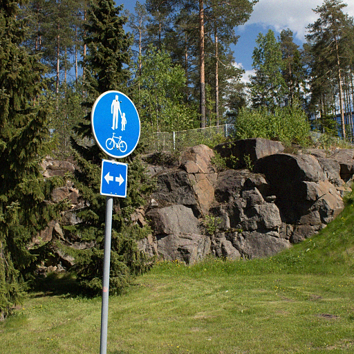
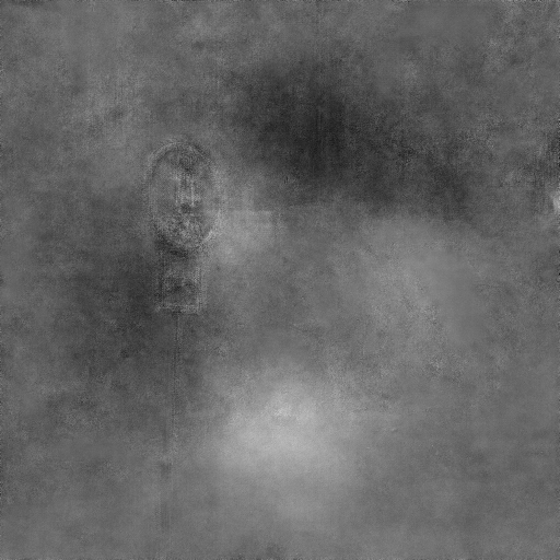
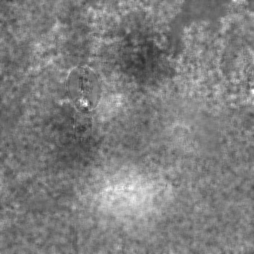
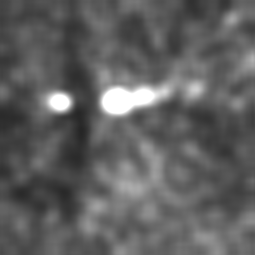
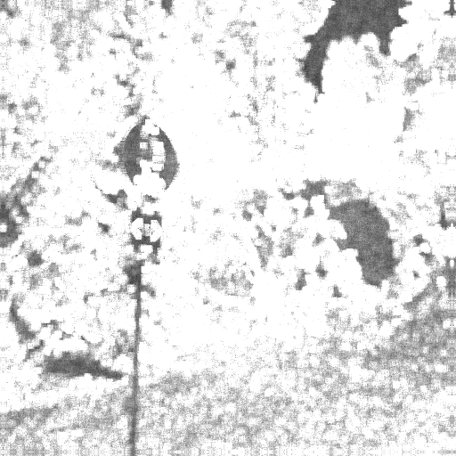
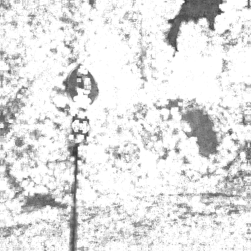
Ground truth	Noisy	SDNet	VDNet	DCAE	RHDCT	LADCT
$\sigma_{av}$=5	image	$\varepsilon_{m}$=0.12	$\varepsilon_{m}$=0.27	$\varepsilon_{m}$=0.44	$\varepsilon_{m}$=2.0	$\varepsilon_{m}$=2.2

Figure 2: Ground truth sigma-map and the results of its estimation from the noisy image by different methods

Image fragments $\boldsymbol{I}$ for generation of patches are selected in the following way. First, a random image from the training set is extracted. Next, a fragment of size 128x128 is cropped from this image to increase the presence of patches with fine details and textures in the training set. This is done by the algorithm described in [40] (selecting three image fragments). To decrease over-learning, random rotations (on $90^{\circ}$, $180^{\circ}$, $270^{\circ}$) and mirroring of selected fragments are used.

The half of input patches $\boldsymbol{P}$ are clipped by restricting pixel values to be in the [0…255] interval. This is done to make a pre-trained SDNet effective for both clipped and non-clipped noise cases.

The design and training of SDNet has been carried out in Matlab R2021a, using the custom training loop. Overall, 150000 iterations with minibatch size 32 were performed. MSE has been used as a loss function to provide smaller number of outliers in sigma-map estimates. Adam optimizer was used with the learning rate $10^{-5}$ for the first 100000 iterations and $5*10^{-6}$ for the last 50000 iterations.

II-D Modification to color images

SDNet has been separately trained for color and grayscale images. To provide a compatibility with the setup used in [22], for color images, noise was independently added to each color component image according to (5) and by using the same sigma-map.

III Numerical Analysis:Sigma-map Estimation

In this section, we analyze a quality of sigma-maps estimation by the pre-trained SDNet. A set of 24 color images (22 images from Tampere17 dataset [21] in addition to Barbara and Baboon images) are selected for testing. Three non-stationary sigma-map models introduced in [22] are used to create a noisy test set. We have multiplied these sigma-maps by a factor to provide necessary mean variance $\sigma_{av}^{2}$ of a sigma-map. Thus, 72 noisy images are generated for each $\sigma_{av}$ value.

III-A Quality of estimation of sigma-map for non-stationary noise

We have used $\varepsilon_{m}$ defined in (2) as a qualitative criterion ($n=72$). The relative errors are demonstrated in Table II, to compare quality of sigma-map estimation by the proposed method SDNet, methods RHDCT [24], LADCT [23], DCAE [25], and the state-of-the-art VDNet [22].

In Table II we have also presented a grayscale modification of SDNet (’SDNet grayscale’) for the comparison. Here sigma-maps are separately estimated for image color channels and then averaged. It is worth noting that estimation of noise for small $\sigma_{m}$ is a difficult task. As one can see from the results provided by RHDCT and LADCT (see example in Fig.2), these methods do not provide satisfactory results, producing relative error values larger than 1.

TABLE I: Image denoising in the case of non-stationary noise, PSNR, dB and SSIM

$\sigma_{av}$	Noisy images		CBDNet (blind)		DnCNN (blind)		VDNet		FFDNet+ color SDNet		FFDNet + true sigma-map		DRUNet+ VDNet		DRUNet+ grayscale SDNet		DRUNet+ color SDNet		DRUNet+ true sigma map
	PSNR	SSIM	PSNR	SSIM	PSNR	SSIM	PSNR	SSIM	PSNR	SSIM	PSNR	SSIM	PSNR	SSIM	PSNR	SSIM	PSNR	SSIM	PSNR	SSIM
5	34.2	0.953	31.7	0.950	34.1	0.973	37.0	0.981	36.5	0.980	36.8	0.981	37.1	0.981	37.5	0.982	37.5	0.983	38.1	0.984
7	31.3	0.919	31.5	0.947	33.3	0.966	35.3	0.973	35.0	0.971	35.2	0.973	35.5	0.974	35.6	0.975	35.8	0.975	36.1	0.977
10	28.3	0.864	31.0	0.938	32.1	0.954	33.5	0.961	33.2	0.959	33.3	0.959	33.7	0.962	33.7	0.963	33.9	0.963	34.1	0.964
15	24.8	0.774	29.8	0.917	30.5	0.933	31.4	0.941	31.1	0.936	31.2	0.936	31.6	0.940	31.6	0.941	31.7	0.942	31.8	0.943
20	22.4	0.693	28.6	0.893	29.3	0.912	29.9	0.920	29.6	0.912	29.7	0.912	30.0	0.918	30.1	0.919	30.1	0.920	30.2	0.920
30	19.1	0.562	26.8	0.847	27.4	0.870	27.8	0.880	27.5	0.863	27.5	0.864	27.9	0.876	27.9	0.875	27.8	0.876	27.9	0.876
45	16.0	0.424	25.0	0.783	25.3	0.813	25.6	0.826	25.1	0.793	25.1	0.794	25.7	0.820	25.5	0.811	25.4	0.812	25.5	0.813

TABLE II: Relative estimation error $\varepsilon_{m}$ of sigma-maps

$\sigma_{av}$	LADCT	RHDCT	DCAE	VDNet	SDNet grayscale	SDNet color
5	1.87	1.69	0.41	0.31	0.27	0.21
7	1.24	1.11	0.32	0.21	0.19	0.13
10	0.80	0.69	0.28	0.15	0.14	0.08
15	0.49	0.40	0.22	0.11	0.08	0.05
20	0.35	0.27	0.21	0.10	0.06	0.04
30	0.24	0.19	0.25	0.11	0.04	0.03
45	0.20	0.19	0.31	0.13	0.03	0.03

III-B Quality of estimation of standard deviation of AWGN

The proposed SDNet can be applied for a special case when all $\sigma_{i,j}=\sigma$, which corresponds to the case of i.i.d. Gaussian noise model.

For a comparative amalysis we have selected three methods: IEDD [21], PCA [20] and WTP [41], which are state-of-the-art for estimation of standard deviation (STD) of AWGN. We have also included in this analysis VDNet [22]. Estimated STD for a given image by SDNet and VDNet methods are calculated as medians of the corresponding estimated sigma-maps.

As a quality criterion we used a relative error of estimation of STD, defined by:

$$\varepsilon=\frac{||\boldsymbol{\sigma_{e}}-\sigma_{t}||_{2}}{n\sigma_{t}}$$ (6)

where $\sigma_{t}$ is a true value of AWGN STD, $n$ is a number of estimates (here $n=24$), $\boldsymbol{\sigma_{e}}$ is a vector of estimated standard deviations for test images. Both clipped and non-clipped noise are considered in this analysis (see Tables III and IV).

SDNet attains the best accuracy, outperforming other methods almost for all cases. Moreover, for $\sigma_{t}$ equal to 3 and 5, SDNet estimation error is twice smaller than that of the nearest competitor. It is interesting to observe that all four methods IEDD, PCA, WTP and VDNet fail for large $\sigma_{t}$ for clipped noise case (values are marked in Table IV in italic and underlined), while SDNet demonstrates very good accuracy both for clipped and non-clipped noise cases.

IV Numerical Analysis: Denoising Using Estimated Sigma-map

Here we use estimated sigma-maps in image denoising. Comparing denoised images obtained by the different sigma-map estimators, we show how much one can boost the performance of denoising by improving accuracy of sigma-map estimation. As denoisers in this study we use DRUNet and FFDNet[13], since their network architecture accepts noise sigma-map as an auxiliary input. Three state-of-the-art CNN-based blind denoising methods, DnCNN[12], CBDNet[14] and VDNet, have been selected for the comparison. The peak signal-to-noise ratio (PSNR) and structural similarity index measure (SSIM) are used as quality criteria.

Note that DnCNN was originally designed to address the problem of Gaussian denoising with unknown noise level, while CBDNet is taking one step further and includes real-world noisy-clean image pairs as training input to estimate more realistic noise models. VDNet is also trained to handle a non-stationary noise, it can simultaneously estimate sigma-map and perform blind denoising. Table I shows average PSNR and SSIM values for 72 denoised test images. Furthermore, for denoisers equipped with the sigma-map estimation by the proposed SDNet, we provide also the results for ideal case of the denoising when the true sigma-map are used. Small differences between PSNR and SSIM values of the results produced by the denoisers accepting true sigma-map with the same denoisers accepting SDNet estimated sigma-map, demonstrate the high accuracy of sigma-map estimation and its influence on denoising performance. As one can see from Table I, a combination of SDNet with DRUNet yields the best denoising performance,and the gap between best results and the results from ideal case (using true sigma-maps) is less than 0.6 db in PSNR and none in SSIM. Although the same comparison is performed for the case of FFDNet denoiser and the gap is smaller, quality of denoising using FFDNet is about 1 db lower than that of DRUNet. In the case of blind denoisers, quality of denoised images is much lower, within the range of 2 $\sim$ 6 dB for low noise levels. It is also interesting that for small noise levels DRUNet with sigma map estimated by VDNet provides better results then VDNet denoiser trained jointly with the sigma-map estimation network. One can observe from the denoised images that blind denoisers can distort texture and eliminating fine details of an image. Denoising based on sigma-map estimated by the proposed SDNet overcomes this problem and preserves fine image details in the low noise levels.

TABLE III: $\varepsilon$ for non-clipped AWGN

true $\sigma$	IEDD	PCA	WTP	VDNet	SDNet
3	0.407	0.573	0.508	1.783	0.200
5	0.204	0.272	0.271	0.906	0.106
7	0.110	0.167	0.176	0.560	0.073
10	0.054	0.098	0.126	0.325	0.043
15	0.033	0.057	0.079	0.171	0.028
20	0.021	0.044	0.057	0.110	0.029
30	0.014	0.031	0.029	0.063	0.018
50	0.013	0.022	0.012	0.040	0.011
75	0.013	0.023	0.007	0.032	0.007

TABLE IV: $\varepsilon$ for clipped AWGN

true $\sigma$	IEDD	PCA	WTP	VDNet	SDNet
3	0.407	0.573	0.507	1.782	0.200
5	0.204	0.274	0.269	0.905	0.110
7	0.114	0.166	0.174	0.559	0.076
10	0.073	0.097	0.122	0.323	0.043
15	0.071	0.053	0.075	0.168	0.026
20	0.077	0.038	0.057	0.105	0.027
30	0.114	0.036	0.055	0.066	0.017
50	0.157	0.069	0.103	0.089	0.014
75	0.207	0.172	0.176	0.150	0.010

V Conclusion

We propose an effective CNN-based method, SDNet, for sigma-map estimation. Advantages of this CNN architecture were discussed. The training set generation and selection of training patches were described.
We have compared the proposed method with the state-of-the-art methods. The results show that SDNet outperforms them in estimation accuracy for both sigma-maps and standard deviation of AWGN, and for both clipped and non-clipped noise cases. For small levels of noise estimation errors for SDNet in average are twice smaller than those of nearest competitors.

A comparative analysis of denoising efficiency using estimated sigma maps demonstrates that the combination of SDNet and DRUNet provides the state-of-the-art quality of image denoising which is very close to the ideal case (where true sigma-maps are used).

References

- [1] J. Astola and P. Kuosmanen, Fundamentals of nonlinear digital filtering. CRC press, 2020.
- [2] V. Lukin, R. Oktem, N. Ponomarenko, and K. Egiazarian, “Image filtering based on discrete cosine transform,” Telecommunications and Radio Engineering, vol. 66, no. 18, pp. 1685–1701, 2007.
- [3] O. B. Pogrebnyak and V. V. Lukin, “Wiener discrete cosine transform-based image filtering,” Journal of Electronic Imaging, vol. 21, no. 4, p. 043020, 2012.
- [4] A. Foi, V. Katkovnik, and K. Egiazarian, “Pointwise shape-adaptive dct for high-quality denoising and deblocking of grayscale and color images,” IEEE transactions on image processing, vol. 16, no. 5, pp. 1395–1411, 2007.
- [5] R. Oktem, L. Yarovslavsky, and K. Egiazarian, “Signal and image denoising in transform domain and wavelet shrinkage: A comparative study,” in 9th European Signal Processing Conference (EUSIPCO 1998). IEEE, 1998, pp. 1–4.
- [6] D. L. Donoho and I. M. Johnstone, “Minimax estimation via wavelet shrinkage,” The annals of Statistics, vol. 26, no. 3, pp. 879–921, 1998.
- [7] J. Portilla, V. Strela, M. J. Wainwright, and E. P. Simoncelli, “Image denoising using scale mixtures of gaussians in the wavelet domain,” IEEE Transactions on Image processing, vol. 12, no. 11, pp. 1338–1351, 2003.
- [8] K. Dabov, A. Foi, V. Katkovnik, and K. Egiazarian, “Image denoising by sparse 3-d transform-domain collaborative filtering,” IEEE Transactions on image processing, vol. 16, no. 8, pp. 2080–2095, 2007.
- [9] A. Buades, B. Coll, and J. M. Morel, “On image denoising methods,” CMLA Preprint, vol. 5, 2004.
- [10] M. Mahmoudi and G. Sapiro, “Fast image and video denoising via nonlocal means of similar neighborhoods,” IEEE signal processing letters, vol. 12, no. 12, pp. 839–842, 2005.
- [11] V. Jain and S. Seung, “Natural image denoising with convolutional networks,” Advances in neural information processing systems, vol. 21, pp. 769–776, 2008.
- [12] K. Zhang, W. Zuo, Y. Chen, D. Meng, and L. Zhang, “Beyond a gaussian denoiser: Residual learning of deep cnn for image denoising,” IEEE transactions on image processing, vol. 26, no. 7, pp. 3142–3155, 2017.
- [13] K. Zhang, W. Zuo, and L. Zhang, “Ffdnet: Toward a fast and flexible solution for cnn-based image denoising,” IEEE Transactions on Image Processing, vol. 27, no. 9, pp. 4608–4622, 2018.
- [14] S. Guo, Z. Yan, K. Zhang, W. Zuo, and L. Zhang, “Toward convolutional blind denoising of real photographs,” in Proceedings of the IEEE/CVF Conference on Computer Vision and Pattern Recognition, 2019, pp. 1712–1722.
- [15] J. Chen, J. Chen, H. Chao, and M. Yang, “Image blind denoising with generative adversarial network based noise modeling,” in Proceedings of the IEEE Conference on Computer Vision and Pattern Recognition, 2018, pp. 3155–3164.
- [16] K. Isogawa, T. Ida, T. Shiodera, and T. Takeguchi, “Deep shrinkage convolutional neural network for adaptive noise reduction,” IEEE Signal Processing Letters, vol. 25, no. 2, pp. 224–228, 2017.
- [17] Y. Wang, X. Song, and K. Chen, “Channel and space attention neural network for image denoising,” IEEE Signal Processing Letters, vol. 28, pp. 424–428, 2021.
- [18] A. Danielyan and A. Foi, “Noise variance estimation in nonlocal transform domain,” in 2009 International Workshop on Local and Non-Local Approximation in Image Processing. IEEE, 2009, pp. 41–45.
- [19] X. Liu, M. Tanaka, and M. Okutomi, “Noise level estimation using weak textured patches of a single noisy image,” in 2012 19th IEEE International Conference on Image Processing. IEEE, 2012, pp. 665–668.
- [20] S. Pyatykh, J. Hesser, and L. Zheng, “Image noise level estimation by principal component analysis,” IEEE transactions on image processing, vol. 22, no. 2, pp. 687–699, 2012.
- [21] M. Ponomarenko, N. Gapon, V. Voronin, and K. Egiazarian, “Blind estimation of white gaussian noise variance in highly textured images,” Electronic Imaging, vol. 2018, no. 13, pp. 382–1, 2018.
- [22] Z. Yue, H. Yong, Q. Zhao, L. Zhang, and D. Meng, “Variational denoising network: Toward blind noise modeling and removal,” arXiv preprint arXiv:1908.11314, 2019.
- [23] V. V. Lukin, D. V. Fevralev, N. N. Ponomarenko, S. K. Abramov, O. B. Pogrebnyak, K. O. Egiazarian, and J. T. Astola, “Discrete cosine transform- based local adaptive filtering of images corrupted by nonstationary noise,” Journal of Electronic Imaging, vol. 19, no. 2, p. 023007, 2010.
- [24] A. A. Shulev, A. Gotchev, A. Foi, and I. R. Roussev, “Threshold selection in transform-domain denoising of speckle pattern fringes,” in Holography 2005: International Conference on Holography, Optical Recording, and Processing of Information, vol. 6252. International Society for Optics and Photonics, 2006, p. 625220.
- [25] S. G. Bahncmiri, M. Ponomarenko, and K. Egiazarian, “Deep convolutional autoencoder for estimation of nonstationary noise in images,” in 2019 8th European Workshop on Visual Information Processing (EUVIP). IEEE, 2019, pp. 238–243.
- [26] O. Ronneberger, P. Fischer, and T. Brox, “U-net: Convolutional networks for biomedical image segmentation,” in International Conference on Medical image computing and computer-assisted intervention. Springer, 2015, pp. 234–241.
- [27] K. He, X. Zhang, S. Ren, and J. Sun, “Deep residual learning for image recognition,” in Proceedings of the IEEE conference on computer vision and pattern recognition, 2016, pp. 770–778.
- [28] K. Zhang, Y. Li, W. Zuo, L. Zhang, L. Van Gool, and R. Timofte, “Plug-and-play image restoration with deep denoiser prior,” arXiv preprint arXiv:2008.13751, 2020.
- [29] V. Hosu, H. Lin, T. Sziranyi, and D. Saupe, “Koniq-10k: An ecologically valid database for deep learning of blind image quality assessment,” IEEE Transactions on Image Processing, vol. 29, pp. 4041–4056, 2020.
- [30] Z. Ying, H. Niu, P. Gupta, D. Mahajan, D. Ghadiyaram, and A. Bovik, “From patches to pictures (paq-2-piq): Mapping the perceptual space of picture quality,” in Proceedings of the IEEE/CVF Conference on Computer Vision and Pattern Recognition, 2020, pp. 3575–3585.
- [31] N. Ponomarenko, O. Eremeev, V. Lukin, and K. Egiazarian, “Statistical evaluation of no-reference image visual quality metrics,” in 2010 2nd European Workshop on Visual Information Processing (EUVIP). IEEE, 2010, pp. 50–54.
- [32] Y. Fang, H. Zhu, Y. Zeng, K. Ma, and Z. Wang, “Perceptual quality assessment of smartphone photography,” in Proceedings of the IEEE/CVF Conference on Computer Vision and Pattern Recognition, 2020, pp. 3677–3686.
- [33] A. Kaipio, M. Ponomarenko, and K. Egiazarian, “Merging of mos of large image databases for no-reference image visual quality assessment,” in 2020 IEEE 22nd International Workshop on Multimedia Signal Processing (MMSP). IEEE, 2020, pp. 1–6.
- [34] B. Lim, S. Son, H. Kim, S. Nah, and K. Mu Lee, “Enhanced deep residual networks for single image super-resolution,” in Proceedings of the IEEE conference on computer vision and pattern recognition workshops, 2017, pp. 136–144.
- [35] K. Ma, Z. Duanmu, Q. Wu, Z. Wang, H. Yong, H. Li, and L. Zhang, “Waterloo Exploration Database: New challenges for image quality assessment models,” IEEE Transactions on Image Processing, vol. 26, no. 2, pp. 1004–1016, Feb. 2017.
- [36] E. Agustsson and R. Timofte, “Ntire 2017 challenge on single image super-resolution: Dataset and study,” in Proceedings of the IEEE conference on computer vision and pattern recognition workshops, 2017, pp. 126–135.
- [37] D. Ghadiyaram and A. C. Bovik, “Massive online crowdsourced study of subjective and objective picture quality,” IEEE Transactions on Image Processing, vol. 25, no. 1, pp. 372–387, 2015.
- [38] M. Ponomarenko, S. G. Bahnemiri, K. Egiazarian, O. Ieremeiev, V. Lukin, V.-T. Peltoketo, and J. Hakala, “Color image database htid for verification of no-reference metrics: Peculiarities and preliminary results,” in 2021 9th European Workshop on Visual Information Processing (EUVIP). IEEE, 2021, pp. 1–6.
- [39] V. V. Lukin, S. K. Abramov, N. N. Ponomarenko, M. L. Uss, M. S. Zriakhov, B. Vozel, K. Chehdi, and J. T. Astola, “Methods and automatic procedures for processing images based on blind evaluation of noise type and characteristics,” Journal of applied remote sensing, vol. 5, no. 1, p. 053502, 2011.
- [40] M. Ponomarenko, S. G. Bahnemiri, and K. Egiazarian, “Deep convolutional network for spatially correlated rayleigh noise suppression on terrasar-x images,” in 2020 IEEE Ukrainian Microwave Week (UkrMW). IEEE, 2020, pp. 458–463.
- [41] X. Liu, M. Tanaka, and M. Okutomi, “Noise level estimation using weak textured patches of a single noisy image,” in 2012 19th IEEE International Conference on Image Processing. IEEE, 2012, pp. 665–668.