Edge but not Least: Cross-View Graph Pooling

Abstract

Graph neural networks have emerged as a powerful model for graph representation learning to undertake graph-level prediction tasks. Various graph pooling methods have been developed to coarsen an input graph into a succinct graph-level representation through aggregating node embeddings obtained via graph convolution. However, most graph pooling methods are heavily node-centric and are unable to fully leverage the crucial information contained in global graph structure. This paper presents a cross-view graph pooling (Co-Pooling) method to better exploit crucial graph structure information. The proposed Co-Pooling fuses pooled representations learnt from both node view and edge view. Through cross-view interaction, edge-view pooling and node-view pooling seamlessly reinforce each other to learn more informative graph-level representations. Co-Pooling has the advantage of handling various graphs with different types of node attributes. Extensive experiments on a total of 15 graph benchmark datasets validate the effectiveness of our proposed method, demonstrating its superior performance over state-of-the-art pooling methods on both graph classification and graph regression tasks.

I Introduction

Graph-structured data is becoming ubiquitous across a wide variety of domains, such as chemical molecules [1], social networks [2, 3], financial networks [4], and citation networks [5]. Learning effective graph representations plays a crucial role for many tasks across various application areas, such as drug discovery [6], molecule property prediction [7], traffic forecast [8], and so on. Recently, graph neural networks (GNN) have emerged as state-of-the-art models for graph representation learning, including graph convolutional network (GCN)[9], graph attention network (GAT) [10], graph isomorphism network (GIN) [11], and GraphSAGE [12]. The majority of these GNN models rely on message passing schemes in graph convolution to learn the embedding of each node by aggregating and transforming the embeddings of its neighbouring nodes. To obtain the representation of the entire graph, node embeddings are aggregated via a readout function or graph pooling methods [13, 14, 15, 16]. Graph pooling methods focus on coarsening an input graph into a compact vector-based representation for the entire graph, which is used for graph prediction tasks, such as graph classification or graph regression.

Figure 1: Classification accuracy on PROTEINS dataset with different edge ratios. (a) The classification accuracy does not significantly drop as we randomly drop different ratios of edges. (b) The classification accuracy does not significantly change when we randomly add different ratios of edges from no-edge graphs. Better view in colors.

To learn informative graph representations, a myriad of graph pooling methods have been proposed, which can be roughly categorized as node sampling based pooling and node clustering based pooling. Node sampling based pooling methods (e.g., SAGPool [17], ASAP [15], HGPSL [13]) typically calculate an importance score for each node and select the top $K$ important nodes to generate an induced subgraph. For example, SAGPool [17] selects nodes by learning importance scores via a self-attention mechanism. HGPSL [13] samples the important nodes and uses an additional structure learning mechanism to learn new graph structure for sampled nodes. Node clustering based pooling methods, like differentiable graph pooling (DiffPool) [14], learn an assignment matrix to cluster nodes into several super-nodes level by level. Through this process, a hierarchy of the induced subgraphs can be generated for representing the whole graph. However, we argue that the existing pooling methods focus primarily on aggregating node-level information for learning graph-level representations, but they fail to exploit the key graph structure. The loss of information present in the global graph structure would further hinder the message passing in subsequent layers.

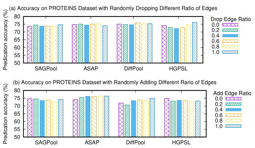
To verify our argument, we selected four state-of-the-art pooling methods: SAGPool [17], ASAP [15], DiffPool [14], and HGPSL [13] and analyzed the influence of changing graph topological structure on the graph classification accuracy. We used the PROTEINS dataset as a case study, where we randomly dropped and added edges with different ratios. As shown in Fig. 1, we found that the random edge manipulation does not cause a significant decrease in the graph classification accuracy. Surprisingly, when there are no edges at all, i.e. dropping 100% edges in Fig 1(a) and adding 0% edges (no edges) in Fig 1(b), the classification accuracy still retains at the same level with other edge ratios. Especially for HGPSL that implicitly uses edge information, the classification accuracy is the highest when all edges are removed. Our empirical studies indicate the current graph pooling methods are heavily node-centric and are unable to fully leverage the crucial information contained in graph structure.

To fill this research gap, we propose a novel cross-view graph pooling method called Co-Pooling that explicitly exploits graph structure for learning graph-level representations. Our main motivations are twofold. First, we would like to capture crucial graph structure through explicitly pruning unimportant edges. Key structure information, such as functional groups (i.e., rings) in bio-molecular networks, or cliques in protein-protein interaction networks and social networks, has been widely recognised as a crucial source for graph prediction tasks [18]. Second, real-world graphs may have various properties such as one-hot node attributes, real-valued node attributes, or even no attributes (see Table I). Hence, we would like our new pooling method to seamlessly handle different types of graphs and make the best of node-level information when available.

Specifically, Co-Pooling is comprised of two key components: edge-view pooling and node-view pooling. The aim of edge-view pooling is to preserve crucial graph structure, which can benefit subsequent graph prediction tasks. This is achieved by capturing high-order structural information via generalized PageRank and pruning the edges with lower proximity weights. For node-view pooling, the importance score for each node is computed and the top important nodes are selected for pooling. The learning of graph pooling from edge and node views seamlessly reinforces each other through exchanging the proximity weights and the selected important nodes. The final pooled graph is obtained by fusing graph representations learnt from two views. Through cross-view interaction, Co-Pooling enables edge-view pooling and node-view pooling to complement each other towards learning effective graph representations.

Our contributions are summarised as follows:

1. We empirically analyze the ineffectiveness of the existing node-centric graph pooling methods in fully leveraging graph structure.

2. We propose a new cross-view graph pooling (Co-Pooling) method to learn graph representations by fusing the pooled graph information from both node view and edge view. The proposed method has the flexibility to handle different types of graphs (labeled/attributed graphs and plain graphs).

3. We verify the effectiveness of Co-Pooling in graph classification and regression tasks across a wide range of 15 graph benchmark datasets, demonstrating its superiority over state-of-the-art pooling methods.

Figure 2: Overview of our proposed cross-view graph pooling. From the edge view, the higher-order structural information is captured via generalized PageRank and the proximity matrix is calculated to prune less important edges. From the node view, the top important nodes are selected for pooling. Edge-view pooling and node-view pooling seamlessly reinforce each other through view interaction. The pooled representations from both views are fused to form the final graph-level representation.

II Related Work

Graph pooling is a key component in GNNs for learning a vector representation of the whole graph. The existing graph pooling methods can be divided into two categories: sampling based pooling and clustering based pooling.

Sampling based pooling methods generate a smaller induced graph by selecting the top important nodes according to certain importance scores of nodes. There has been a series of graph pooling methods that fall into this category. Gao et al. [19] proposed a pooling method that selects the top-$k$ nodes to form a smaller graph. This method projects node features into scalar values and uses them as the node selection criterion. Similarly, SAGPool [17] employs a self-attention mechanism to calculate the importance score for each node, and then chooses the top-ranked nodes to induce the pooled graph. Ranjan et al. [15] proposed adaptive structure aware pooling (ASAP) for learning graph representations. This method updates node embeddings by aggregating features of neighbouring nodes in a local region. After that, a fitness score for the updated node is calculated to select the top-$k$ nodes to form the pooled graph. These methods, however, do not leverage graph structure in the pooling process. HGPSL [13] takes a step forward to learn new edges between the top important nodes selected for the pooled graph. However, this method does not preserve the structure information contained in the original graph.

On the other hand, clustering based pooling methods learn an assignment matrix to cluster nodes into super-nodes. DiffPool [14] learns a differentiable soft cluster assignment for nodes in an end-to-end manner. The learnt assignment is used for grouping nodes in the last layer to several clusters in the subsequent layer. HaarPooling [20] relies on compressive Haar transform filters to generate the induced graph of smaller size.

Most of the existing pooling methods operate on a single node view; they are unable to fully leverage crucial graph structure. Although preliminary attempts (e.g., EdgePool [21] and EdgeCut [22]) have been made to pool the input graph from an edge view, these methods simply rely on local connectivity to calculate pairwise edge scores and suffer from high computational complexity. In contrast, our edge-view pooling mechanism leverages higher-order structure information to assess the importance of edges, which is fed to further guide the selection of important nodes for node-view pooling. To the best of our knowledge, our work is the first to propose a cross-view graph pooling method, which enables us to fuse useful information from both edge and node views towards learning effective graph-level representations.

III Method

This section presents the overview of our proposed cross-view graph pooling, followed by a detailed description of the main components.

III-A Preliminaries

We first define notations to clarify the description of our proposed method. Assume we have $m$ input graphs $\mathbb{G}=\{G^{(0)},G^{(1)},\cdots,G^{(m)}\}$ and their corresponding targets $\mathbb{Y}=\{y^{(0)},y^{(1)},\cdots,y^{(m)}\}$. For graph classification, $y_{i}$ is a discrete class label; for graph regression, $y_{i}$ is a continuous regression target variable $y_{i}\in\mathbb{R}$. A graph $G^{(g)}$ is represented as $(\mathbf{X}^{(g)},\mathbf{A}^{(g)})$, where $\mathbf{X}^{(g)}\in\mathbb{R}^{n\times d}$ represents the node attribute matrix, where $n$ is the number of nodes and $d$ is the dimension of node attributes; $\mathbf{A}^{(g)}$ is the adjacent matrix, if there is an edge between node $i$ and node $j$, $\mathbf{A}^{g}_{ij}=1$; otherwise $\mathbf{A}^{g}_{ij}=0$ . For simplicity, $(\mathbf{X}^{(g)},\mathbf{A}^{(g)})$ is also noted as $(\mathbf{X},\mathbf{A})$ to represent an arbitrary graph. $\hat{\mathbf{A}}=\mathbf{A}+\mathbf{I}$ stands for the adjacent matrix with self-loops.

In this paper, we use graph convolution network (GCN) as our backbone to learn representations for graphs. The graph convolution operation is defined as:

$$\mathbf{H}=\hat{\mathbf{D}}^{-1/2}\hat{\mathbf{A}}\hat{\mathbf{D}}^{-1/2}\mathbf{X}\mathbf{\Theta}$$ (1)

where $\mathbf{H}\in\mathbb{R}^{n\times f}$ is node embedding after convolution, $f$ is the dimension of node embedding; $\hat{\mathbf{D}}_{ii}=\sum_{j=0}\hat{\mathbf{A}}_{ij}$ is diagonal degree matrix; $\mathbf{\Theta}$ is a learnable parameter. After node embeddings $\mathbf{H}$ are learnt, graph pooling operation is applied to aggregate node embeddings to form a vector representation for the whole graph. This graph-level representation can be used for downstream graph prediction tasks, i.e. graph classification and graph regression.

III-B Cross-View Graph Pooling

The proposed cross-view graph pooling (Co-Pooling) consists of two main components: edge-view pooling and node-view pooling, as illustrated in Fig. 2, Co-Pooling simultaneously performs pooling from both edge view and node view. Through cross-view interaction, edge-view pooling and node-view pooling seamlessly reinforce each other, and finally the pooled graphs from two views are fused to form the final graph representation.

III-B1 Edge-View Pooling

The key objective of edge-view pooling is to preserve crucial information contained in graph structure. This is achieved by capturing high-order structural information via generalized PageRank (GPR) [23] and pruning unimportant edges. Through edge-view pooling, the learnt representation captures a better connectivity relationship between nodes and higher-order graph structure information.

Specifically, we first update node embeddings by generalized PageRank to capture the information from higher-hop neighbours. As shown in Eq. (2), the node embeddings are updated by multiplying different GPR weights $\beta_{t}$. When $t=0$, we have $\mathbf{H}^{0}=\mathbf{H}$; while $t>0$, we have $\mathbf{H}^{t}=\hat{\mathbf{D}}^{-1/2}\hat{\mathbf{A}}\hat{\mathbf{D}}^{-1/2}\mathbf{H}^{t-1}$. Through generalized PageRank, node embeddings propagate $T$ steps. For each step, the GPR weight $\beta_{t}$ is learnable. Therefore, the contribution of each propagation step towards node embeddings can be learnt adaptively. The GPR operation of $T$ steps helps to incorporate higher-hop neighbours’ information to update node embeddings.

$$\mathbf{O}=\sum_{t=0}^{T}\beta_{t}\mathbf{H}^{t}$$ (2)

After updating node embeddings by generalized PageRank, we calculate the proximity weights between each pair of nodes, and the edges with low proximity weights can be pruned to only preserve crucial graph structure.

The process of computing the proximity weights can be illustrated using Eq. (3), where $\mathbf{O}_{i}$ and $\mathbf{O}_{j}$ are the GPR updated embeddings of node $i$ and node $j$. We first transform node embeddings $\mathbf{O}_{i}$ and $\mathbf{O}_{j}$ via a linear transformation parameterized with $\mathbf{W}$ and then concatenate the transformed embeddings. Another linear transformation with learnable parameters $\mathbf{a}$ is used to transform the concatenated embeddings. Finally, the proximity weight $\mathbf{P}_{ij}$ between node $i$ and node $j$ is obtained after a Sigmoid function.

$$\mathbf{P}_{ij}=\sigma(\mathbf{a}^{T}[\mathbf{W}\mathbf{O}_{i}\lVert\mathbf{W}\mathbf{O}_{j}])*\mathbf{A}_{ij},$$ (3)

where $\mathbf{P}_{ij}$ is the proximity weight between node $i$ and node $j$; $\sigma$ is Sigmoid function; $\lVert$ represents the concatenation operation; $\mathbf{a}$ and $\mathbf{W}$ are learnable parameters; $\mathbf{A}_{ij}=1\ or\ 0$ indicates whether or not there is an edge connecting node $i$ and node $j$.

According to the proximity weight $\mathbf{P}_{ij}$ of each node pair, we can obtain the proximity matrix $\mathbf{P}$ for all node pairs in a graph. To emphasize the proximity between each node and itself, we update the proximity matrix by adding value 1 in diagonal, i.e., $\mathbf{\hat{P}}=\mathbf{P}+\mathbf{I}$. For undirected graphs, we average the proximity weights at symmetric positions by $\mathbf{P}_{sym}=(\mathbf{\hat{P}}+\mathbf{\hat{P}}^{T})/2$.

Based on the proximity matrix $\mathbf{P}_{sym}$, we prune unimportant edges with low proximity weights in the graph. For a given edge retaining ratio $\gamma$, we have the cut proximity matrix $\mathbf{P}_{cut}=\textrm{Top}_{\gamma}(\mathbf{P}_{sym})$, where $\textrm{Top}_{\gamma}()$ is the operation that retains the top $\gamma$ percentage of edges with high proximity weights. Accordingly, we update the adjacent matrix to reflect the removal of edges. The cut proximity matrix provides a better measure to quantify the higher-order connectivity relationship between nodes, which is fed to node-view pooling to guide the selection of important nodes.

III-B2 Node-View Pooling

For node-view pooling, the aim is to select the top $K$ important nodes for coarsening the input graph. To better measure the connectivity between nodes, we take the cut proximity matrix from edge-view pooling to compute an importance score for each node, given by

$${\mathbf{s}}=\hat{\mathbf{D}_{cut}}^{-1/2}\hat{\mathbf{P}_{cut}}\hat{\mathbf{D}_{cut}}^{-1/2}\mathbf{H}{\mathbf{1}}^{T}$$ (4)

where $\mathbf{s}$ is the score vector for all nodes, $\hat{\mathbf{D}_{cut}}$ is diagonal degree matrix of $\hat{\mathbf{P}_{cut}}$, $\hat{\mathbf{P}_{cut}}=\mathbf{P}_{cut}+\mathbf{I}$, $\mathbf{1}^{T}$ is the vector containing all ones.

Based on nodes’ importance scores, we select the top $K=n*\epsilon$ nodes, where $\epsilon$ is the node pooling ratio. After selecting the nodes, we obtain the $indices$ and embeddings of all selected nodes.

III-B3 Edge-Node View Interaction

To enable edge-view pooling and node-view pooling to reinforce each other, our Co-Pooling method exchanges the cut proximity matrix and the indices of selected nodes, which serve as the mediator for the interaction between two views.

For node-view pooling, the cut proximity matrix from edge-view pooling is used to calculate the important score for each node. The cut proximity matrix better reflects higher-order connectivity relationship between nodes, thus providing more accurate information than the original adjacent matrix to quantify the importance of nodes. After obtaining the node scores, we select the top-K important nodes as the pooled representation from node-view pooling, i.e. $\mathbf{H}(indices,:)$, where $(indices,:)$ represents index selection operation.

For edge-view pooling, the indices of selected nodes obtained from node-view pooling are used to cluster nodes into super-nodes. The important node indices in node-view pooling are useful to guide the clustering operation, as the selected important nodes are determined by considering higher-order structure information. The pooled representation from edge-view pooling is obtained through $\mathbf{P}_{cut}(indices,:)\times\mathbf{O}$, where $\times$ means matrix multiplication.

Lastly, the pooled representations from node-view pooling and edge-view pooling are fused to form the final graph representation as:

$$\mathbf{Z}=\mathbf{W}[\mathbf{P}_{cut}(indices,:)\times\mathbf{O}\lVert\mathbf{H}(indices,:)]$$ (5)

where $\mathbf{W}$ is the learnable parameter for linear transformation; $\lVert$ represents the concatenation operator. $\mathbf{Z}$ is the graph-level representation after pooling. Through edge-node view interaction, our Co-Pooling method enables edge-view pooling and node-view pooling to complement each other towards learning more effective graph representations.

TABLE I: Details of graph datasets for graph classification evaluation.

Data set	# of Graphs	# of Classes	Avg. # of Nodes	Avg. # of Edges	Node Attributes	Dataset Type
BZR-A	405	2	35.75	38.36	Real-valued Attribute	Attributed
AIDS-A	2000	2	15.69	16.20	Real-valued Attribute	Attributed
FRANKENSTEIN	4337	2	16.90	17.88	Real-valued Attribute	Attributed
PROTEINS	1113	2	39.06	72.82	Node label	Labeled
D&D	1178	2	284.32	715.66	Node label	Labeled
NCI1	4110	2	29.87	32.30	Node label	Labeled
NCI109	4127	2	29.68	32.13	Node label	Labeled
MSRC_21	563	20	77.52	198.32	Node label	Labeled
COLLAB	5000	3	74.49	2457.78	None	Plain
IMDB-BINARY	1000	2	19.77	96.53	None	Plain
IMDB-MULTI	1500	3	13.00	65.94	None	Plain
REDDIT-BINARY	2000	2	429.63	497.75	None	Plain
REDDIT-MULTI-12K	11929	11	391.41	456.89	None	Plain

IV Experiments

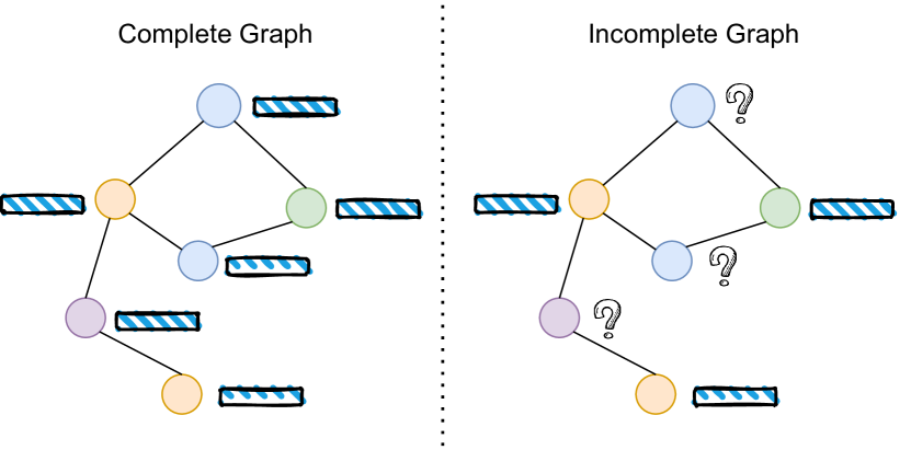
In this section, we validate the performance of our proposed cross-view graph pooling method on both graph classification and graph regression tasks. For graph classification task, we compare our method with several state-of-the-art pooling methods at two settings: complete graphs with various types of node attributes and incomplete graphs. As illustrated in Fig. 3, complete graphs refer to the graphs with all node attributes, while incomplete graphs are the ones with a portion of nodes having completely missing attributes. The incomplete graph setting is used to simulate real-world scenarios where attribute information for some nodes are inaccessible due to privacy or legal constraints. Our method is also compared against baseline pooling methods on graph regression task.

Figure 3: Comparison between complete graphs and incomplete graphs.

IV-A Graph Classification on Complete Graphs

Benchmark Datasets

We conduct graph classification tasks on a total of 13 benchmark graph datasets with various attribute properties, including three attributed graphs with real-valued node attributes, five labeled graphs with only one-hot node attributes, and five plain graphs with no node attributes. The detailed statistics about these datasets are listed in Table I.

• BZR-A [24] is a dataset of chemical compounds for classifying biological activities into active and inactive. The node attributes are 3D coordinates of the compound structures.

• AIDS-A [25] contains graphs representing molecular compounds. It contains two classes of graphs, which are against HIV or not.

• FRANKENSTEIN [26] consists of molecules as mutagens and non-mutagens for mutagenicity classification task. Node attributes are 780 dimensions MNIST [27] image vectors of pixel intensities, which represent chemical atom symbols.

• D&D [28] and PROTEINS [29] include macromolecules as graph datasets in bioinformatics, which are for enzyme and non-enzyme classification task.

• NCI1 [30] and NCI109 [30] contain chemical compounds as small molecules, which are used for anticancer activity classification.

• MSRC_21 [31] is graph dataset constructed by semantic images. Each semantic image is represented as a conditional Markov random field graph. Nodes in a graph represent the segmented superpixels in an image. If the segmented superpixels are adjacent, the corresponding nodes are connected. Each node is assigned with a semantic label as the node attribute.

• COLLAB [2] is a scientific collaboration dataset, where each graph represents the collaboration network of one researcher. The task of COLLAB is to classify the graph into different research fields.

• IMDB-BINARY [2] and IMDB-MULTI [2] are two datasets for classifying each graph into different movie genres. Each graph is an ego-network for each actor/actress, and nodes also represent actors/actresses.

• REDDIT-BINARY [2] and REDDIT-MULTI-12k [2] are two datasets generated from online discussions. Each graph represents a discussion thread where nodes are different users. If one of two users responds to the other one, there is an edge between these two. The task is to classify which section the discussion belongs to.

TABLE II: Graph classification accuracy on benchmark graph datasets by different graph pooling methods. The best results are marked in bold. Higher is better. (- means the results can not be got in an acceptable time, i.e. 24h)

Datasets	SAGPool	ASAP	DiffPool	HGPSL	EdgePool	Co-Pooling/GPR	Co-Pooling/NV	Co-Pooling
BZR-A	82.95$\pm$4.91	83.70$\pm$6.00	83.93$\pm$4.41	83.23$\pm$6.51	83.43$\pm$6.00	81.00$\pm$5.82	81.69$\pm$5.80	85.67$\pm$5.29
AIDS-A	98.85$\pm$0.78	99.00$\pm$0.74	99.40$\pm$0.58	99.10$\pm$0.66	99.05$\pm$0.69	98.85$\pm$0.71	98.90$\pm$0.58	99.45$\pm$0.42
FRANKENSTEIN	60.94$\pm$2.90	66.73$\pm$2.76	65.08$\pm$1.50	62.19$\pm$1.74	62.99$\pm$2.21	64.01$\pm$1.70	67.00$\pm$2.37	64.15$\pm$1.34
D&D	76.91$\pm$3.42	77.84$\pm$3.41	78.01$\pm$2.70	77.33$\pm$4.22	76.66$\pm$2.05	75.81$\pm$3.81	77.00$\pm$5.04	77.85$\pm$2.21
PROTEINS	73.68$\pm$4.63	74.85$\pm$5.18	75.11$\pm$2.95	74.13$\pm$4.12	77.01$\pm$5.41	73.68$\pm$2.33	76.28$\pm$5.09	76.19$\pm$4.13
NCI1	71.51$\pm$4.51	76.59$\pm$1.71	74.14$\pm$1.43	73.48$\pm$2.42	78.39$\pm$2.43	77.25$\pm$2.11	79.15$\pm$2.04	78.66$\pm$1.48
NCI109	69.69$\pm$3.27	74.73$\pm$3.48	72.04$\pm$1.43	72.30$\pm$2.18	77.01$\pm$2.39	75.60$\pm$1.46	78.07$\pm$1.77	77.08$\pm$2.03
MSRC_21	90.22$\pm$2.82	90.41$\pm$3.91	90.41$\pm$3.58	88.97$\pm$4.78	90.05$\pm$3.02	91.64$\pm$2.79	91.29$\pm$3.70	92.54$\pm$2.63
COLLAB	70.58$\pm$2.31	72.84$\pm$1.84	72.18$\pm$1.68	74.2$\pm$2.72	-	74.82$\pm$2.10	68.9$\pm$5.59	77.30$\pm$2.29
IMDB-BINARY	60.9$\pm$2.34	65.5$\pm$2.80	58.27$\pm$5.92	62.5$\pm$3.5	60.3$\pm$5.08	70.4$\pm$3.85	70.8$\pm$3.6	72.1$\pm$4.44
IMDB-MULTI	39.8$\pm$3.39	45.93$\pm$4.03	40.00$\pm$4.52	40.53$\pm$4.88	44.27$\pm$4.50	47.6$\pm$4.55	44.8$\pm$3.94	49.07$\pm$3.28
REDDIT-BINARY	83.55$\pm$4.53	-	84.61$\pm$2.42	-	88.35$\pm$2.31	88.90$\pm$2.00	88.0$\pm$4.69	89.35$\pm$1.25
REDDIT-MULTI-12K	40.56$\pm$3.30	-	41.21$\pm$1.96	-	-	46.84$\pm$2.26	49.02$\pm$1.56	46.85$\pm$2.62

Baselines

We use five state-of-the-art graph pooling methods as our baselines: SAGPool [17], ASAP [15], DiffPool [14], HGPSL [13], and EdgePool [21]. When training DiffPool, we use the auxiliary link prediction loss function and entropy regularization items as did in the original paper. In addition, we also compare with two ablated variants of our cross-view graph pooling (Co-Pooling): Co-Pooling/GPR, and Co-Pooling/NV. Cross-pool/GPR is our cross-view graph pooling without generalized PageRank, and Co-Pooling/NV is our cross-view graph pooling without node-view pooling.

Model Architecture and Training

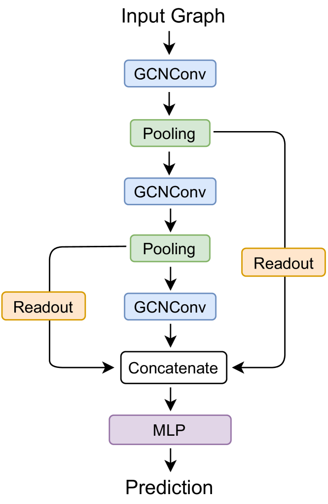
In our experiments, the GNN used is built on the GCN architecture. The whole GNN consists of three GCN layers, two pooling layers and three linear transformation layers. After the last linear transformation layer, the SoftMax classifier is connected. Note that, the input to the first linear transformation layer is the concatenated features after each pooling layer. For all datasets, we use the same GNN architecture for fair comparison. The detailed architecture is provided in Appendix A.

When training the GNN model, we perform 10-fold cross-validation as did in [14]. We randomly split the dataset into training, validation, and test sets with 80%, 10% and 10% graphs. We use Adam [32] optimizer for training the GNN model. The optimization stops if the validation loss does not improve after 50 epochs. The maximum epoch is set as 300. Following the strategy of searching optimal hyperparameters in  [17], we use grid search to obtain optimal hyperparameters for each method. The ranges of different hyperparameters are as follows: learning rate in {0.005, 0.0005, 0.001}; weight decay in {0.0001 0.001}; node pooling ratio in {0.5, 0.25}; hidden size in {128, 64}; dropout ratio in {0, 0.5}. To implement convolution operation on plain graph datasets where nodes have no attributes, we follow the implementation in DiffPool [14] to pad each node with a constant vector, i.e. all-one vector in a fixed dimension.

Classification with State-of-the-art

We compare graph classification accuracy of all methods averaged over 10-fold cross-validation on each dataset. For a fair comparison, all baseline methods and our method are trained using the same training strategy. The GNN model architecture used for each method is also the same. As shown in Table II, our cross-view graph pooling method achieve the best results across 11 datasets and the second place on the other two datasets. Particularly, our method significantly improves the best baseline method by 6.6%, 3.14%, 7.81%, 2.13% and 1.74% on IMDB-BINARY, IMDB-MULTI, REDDIT-MULTI-12K, MSRC_21 and BZR-A, respectively. This proves the effectiveness of our proposed method in predicting different types of graphs with various attribute properties. It is worth noting that our proposed cross-view graph pooling method achieves the best performance on all five datasets without node attributes. This shows the superiority of our method to complement the node-view pooling by edge-view pooling, when node attributes are not informative.

When comparing different variants of our method, Co-Pooling consistently outperforms Co-Pooling/GPR on all datasets. This shows the importance of using generalized PageRank to capture the higher-order structure information. Co-Pooling yields higher accuracy than Co-Pooling/NV on most (8/13) of the datasets. This demonstrates the effectiveness of our method in combining two complementary views. On Labeled graphs, the performance of Co-Pooling and Co-Pooling/NV is comparable. This is because the important node indices used for clustering nodes in edge view may be inaccurate, as one-hot attributes provide limited information. On attributed graphs with real-valued node attributes and plain graphs with padding all-one vectors as node attributes, the obtained important node indices are more accurate to complement edge-view.

IV-B Graph Classification on Incomplete Graphs

We also compare the performance of our method and baseline methods on incomplete graphs. For incomplete graphs, a portion of nodes have completely missing attributes, as shown in Fig. 3. This set of experiments is used to evaluate the effectiveness of our method on real-world scenarios, where attribute information for some nodes are inaccessible due to privacy or legal constraints.

Experimental Setup and Training

We perform experiments on attributed graph AIDS-A and labeled graph MSRC_21 as a case study. For the two datasets, we randomly select different ratios of nodes and remove their original node attributes, while keeping all other remaining nodes unchanged. We define the ratio of nodes with all their attributes removed as incomplete ratio. For example, if we remove all attributes for 10% of nodes, the incomplete ratio is 10%. The resulting incomplete graph datasets are randomly divided into training set (80%), validation set (10%) and test set (10%). We train the GNN model with different pooling methods on training set. The GNN model architecture used in this part is the same as that in Section IV-A. The best hyperparameters obtained from Section IV-A are used for training the GNN model in this part. Model architecture and training strategy for each method remain the same. We report graph classification accuracy averaged over 10-fold cross-validation.

Comparison. with State-of-the-art

Fig. 4 compares the classification accuracy of all methods on MSRC_21 incomplete dataset. For all baseline methods, the classification accuracy drops markedly as the incomplete ratio increases from 0% to 50%. For our Co-Pooling method, the accuracy decreases at a much slower rate than baseline methods. Especially for DiffPool, HGPSL and EdgePool, the classification accuracy drops by 3.73%, 12.33% and 4.61%, respectively, even though only 10% nodes have their attributes missing. Under the 10% incomplete ratio, Co-Pooling and its variants can still achieve at least 77.93% accuracy. Compared with the best baseline method ASAP, Co-Pooling achieves an average of 8.62% increase in classification on all incomplete graph datasets with an incomplete ratio from 0% to 50%.

Figure 4: Graph classification accuracy on incomplete Labeled graph dataset (MSRC_21) by different graph pooling methods. Better view in colors.

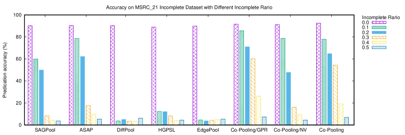
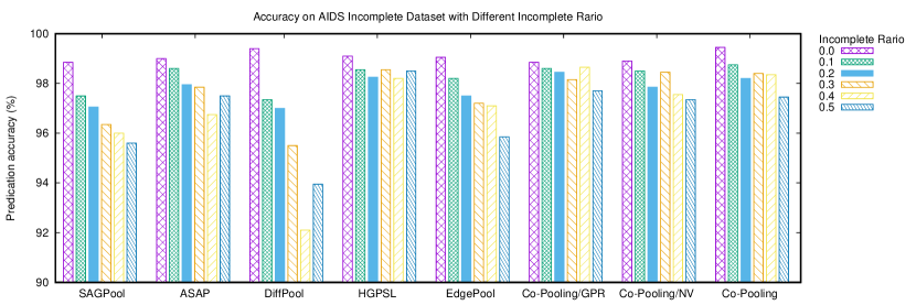
Fig. 5 compares graph classification accuracy of all methods on AIDS-A incomplete datasets. We can see that, for SAGPool, DiffPool and EdgePool, the classification accuracy decreases by 3.25%, 5.45%, and 3.2%, respectively, when the incomplete ratio increases from 0% to 50%. In contrast, the accuracy of our methods drops only by 1.15% under the same setting. Compared with ASAP, our methods can achieve better performance under all incomplete ratios. Compared with HGPSL, our methods achieve better performance on 0%, 10%, 20% and 40% incomplete graph datasets. Overall, our method still outperform HGPSL in terms of the average performance on all incomplete graph datasets,

The classification comparisons on incomplete graph datasets demonstrate the effectiveness of our method in handling graphs with missing node attributes. This further testifies the complementary advantage of our method by fusing node-view and edge-view pooling, especially when node attributes are less informative.

Figure 5: Graph classification accuracy on incomplete attributed graph dataset (AIDS-A) by different graph pooling methods. Better view in colors.

IV-C Parameter Sensitivity

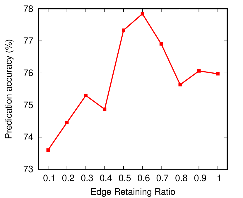
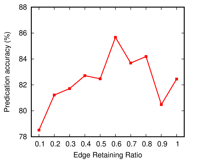
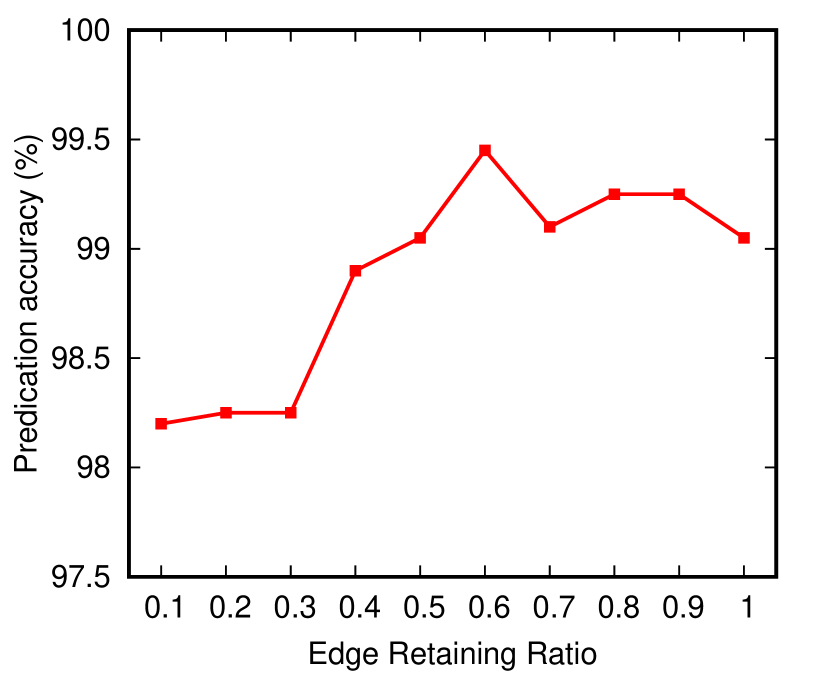
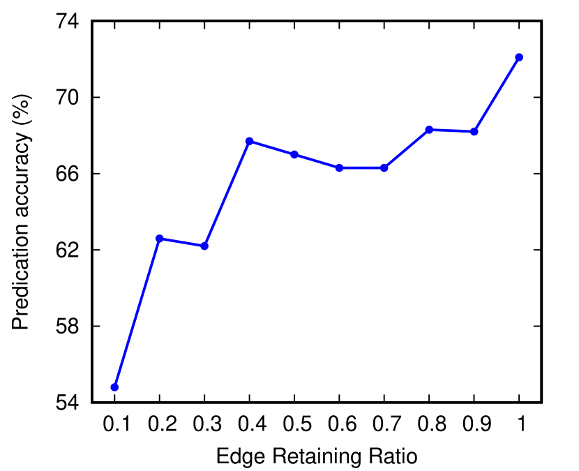
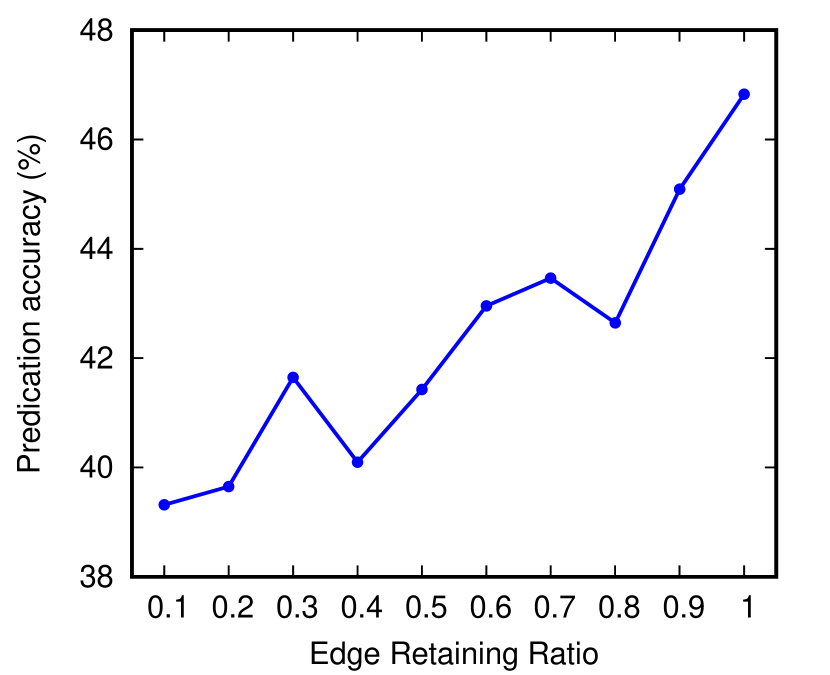
The Co-Pooling method has the edge retaining ratio ($\gamma$) as an important parameter to determine how many percentage of edges are retained during edge-view pooling. To investigate the effect of the edge retaining ratio (i.e., $\gamma$) on the graph classification accuracy of Co-Pooling, we conduct empirical studies on six representative graph datasets, including two labeled graphs, two attributed graphs, and two plain graphs. On each graph dataset, we train the GNN model with the keeping ratio ranging from 10% to 100%. All other hyperparameters are set as the best parameters obtained in Section IV-A. We also use the same GNN model architecture and training strategy as in Section IV-A. We report the average classification accuracy on 10-fold cross-validation.

Fig. 6 plots the change in classification accuracy with respect to $\gamma$ on the six datasets. On the two labeled graphs (PROTEINS and D&D), we find that keeping all edges ($\gamma=1.0$) is not the best choice for graph classification. As shown in Fig. 6(a) and (b), Co-Pooling achieves the highest classification accuracy when $\gamma=0.7$ on PROTEIN, and $\gamma=0.6$ on D&D, respectively. Similarly, this phenomenon can also be observed on the two attributed graphs (BZR-A and AIDS-A). As shown in Fig. 6(c) and (d), Co-Pooling achieves the best performance when $\gamma$ is set to 0.6 on the two datasets. The results on the four datasets indicate not all edges are useful for graph classification when graphs have informative node attributes. Again, this confirms the benefit of our proposed method to preserve crucial edge information through edge-view pooling and use this knowledge to further guide node-view pooling.

In contrast, on the two plain graphs (IMDB-BINARY and REDDIT-MULTI-12K), keeping all edges renders the highest classification accuracy. As shown in Fig. 6 (e) and (f), Co-Pooling achieves the best performance on both graphs when retaining all edges ($\gamma=1.0$). This is what we have expected, because when graphs have no node attributes, the whole graph structure is more critical to graph classification.

(a) PROTEINS

(b) D&D

(c) BZR-A

(d) AIDS-A

(e) IMDB-BINARY

(f) REDDIT-MULTI-12K

Figure 6: Accuracy change on different datasets with different edge retaining ratio ($\gamma$). Better view in colors.

IV-D Graph Regression

Lastly, we also carry out experiments to evaluate the effectiveness of the proposed method in undertaking graph regression task. We compare Co-Pooling with the same state-of-the-art pooling methods on the following two graph datasets:

• ZINC [33, 34] contains 250k molecules and their property values. The task is to regress the property values of input graph. In this experiment, we focus on predicting one graph property, contained solubility. Following the setting in [35], we use 10k graphs from ZINC for training, 1K graphs for validation, and 1K graphs for testing.

• QM9 [36, 37] is a graph dataset consisting of 13k molecules with 19 regression targets. This dataset is originally used in quantum chemistry for regressing the property of molecules. We try to regress dipole moment $\mu$, one of 19 properties. All 13K molecules are randomly divided into 80% training set, 10% validation set and 10% test set.

For training a regression model for each dataset, we use GCN as the backbone GNN and inject two pooling layers before a MLP. Follow the setting in [35], L1 loss function is used for training the model. We use Adam optimizer and learning rate decay policy to optimize the model. The initial learning rate and weight decay are set as 0.001 and 0.0001, respectively. We train the regression model under four different random seeds and report the average mean absolute error (MAE) on the test set.

We compare our Co-Pooling method with SAGPool, ASAP, DiffPool, HGPSL, and EdgePool on the two datasets. As shown in Table III, our Co-Pooling method consistently achieves better regression performance than other baseline methods. Particularly, Co-Pooling outperforms DiffPool and HGPSL by a large margin on both datasets. The experimental results reflect the effectiveness of our method on graph regression task. This concludes that our method is effective in learning a better graph-level representation by fusing edge-view and node-view pooling, leading to competitive performance on both graph classification and regression tasks.

TABLE III: Graph regression task: mean absolute error (MAE) on ZINC dataset and QM9 dataset. Lower is better.

Datasets	ZINC	QM9
GCN+SAGPool	0.378$\pm$0.031	0.545$\pm$0.010
GCN+ASAP	0.372$\pm$0.026	0.500$\pm$0.017
GCN+DiffPool	1.641$\pm$0.026	1.331$\pm$0.014
GCN+HGPSL	1.326$\pm$0.096	1.035$\pm$0.049
GCN+EdgePool	0.382$\pm$0.030	0.489$\pm$0.022
GCN+Co-Pooling (ours)	0.340$\pm$0.036	0.439$\pm$0.009

V Conclusion and Future Work

We proposed a cross-view graph pooling (Co-Pooling) method to learn graph-level representations from both edge view and node view. We argued that most of the existing pooling methods are highly node-centric and they are unable to fully leverage crucial information contained in graph structure. To explicitly exploit graph structure, our proposed method seamlessly fuses the pooled graph information from two views. From the edge view, generalized PageRank is used to aggregate information from higher-hop neighbours to better capture the higher-order graph structure. The proximity weights between node pairs are calculated to prune less important edges. From the node view, the node importance scores are computed through the proximity matrix to select the top important nodes for node-view pooling. The pooled representations from two views are fused together as the final graph representation. Through cross-view interaction, edge-view pooling and node-view pooling complement each other to effectively learn informative graph-level representations. Experiments on a total of 15 graph benchmark datasets demonstrate the superior performance of our method on both graph classification and regression tasks. For future work, we would like to generalize cross-view graph pooling to learn more interpretable graph representations.

Appendix A The graph neural network structure

The network structure for graph classification task is shown in Fig. 7.

Figure 7: Graph neural network structure for graph classification task.

References

- [1] A. K. Debnath, R. L. Lopez de Compadre, G. Debnath, A. J. Shusterman, and C. Hansch, “Structure-activity relationship of mutagenic aromatic and heteroaromatic nitro compounds. correlation with molecular orbital energies and hydrophobicity,” Journal of medicinal chemistry, vol. 34, no. 2, pp. 786–797, 1991.
- [2] P. Yanardag and S. Vishwanathan, “Deep graph kernels,” in Proceedings of the 21th ACM SIGKDD international conference on knowledge discovery and data mining, 2015, pp. 1365–1374.
- [3] B. Rozemberczki, O. Kiss, and R. Sarkar, “An api oriented open-source python framework for unsupervised learning on graphs,” arXiv preprint arXiv:2003.04819, 2020.
- [4] W. L. Hamilton, “Graph representation learning,” Synthesis Lectures on Artifical Intelligence and Machine Learning, vol. 14, no. 3, pp. 1–159, 2020.
- [5] C. Morris, N. M. Kriege, F. Bause, K. Kersting, P. Mutzel, and M. Neumann, “Tudataset: A collection of benchmark datasets for learning with graphs,” arXiv preprint arXiv:2007.08663, 2020.
- [6] D. Jiang, Z. Wu, C.-Y. Hsieh, G. Chen, B. Liao, Z. Wang, C. Shen, D. Cao, J. Wu, and T. Hou, “Could graph neural networks learn better molecular representation for drug discovery? a comparison study of descriptor-based and graph-based models,” Journal of cheminformatics, vol. 13, no. 1, pp. 1–23, 2021.
- [7] J. Li, D. Cai, and X. He, “Learning graph-level representation for drug discovery,” arXiv preprint arXiv:1709.03741, 2017.
- [8] W. Jiang and J. Luo, “Graph neural network for traffic forecasting: A survey,” arXiv preprint arXiv:2101.11174, 2021.
- [9] T. N. Kipf and M. Welling, “Semi-supervised classification with graph convolutional networks,” in International Conference on Learning Representations., 2017.
- [10] P. Veličković, G. Cucurull, A. Casanova, A. Romero, P. Lio, and Y. Bengio, “Graph attention networks,” in International Conference on Learning Representations., 2018.
- [11] K. Xu, W. Hu, J. Leskovec, and S. Jegelka, “How powerful are graph neural networks?” in International Conference on Learning Representations, 2019.
- [12] W. L. Hamilton, R. Ying, and J. Leskovec, “Inductive representation learning on large graphs,” in Proceedings of the 31st International Conference on Neural Information Processing Systems, 2017, pp. 1025–1035.
- [13] Z. Zhang, J. Bu, M. Ester, J. Zhang, C. Yao, Z. Yu, and C. Wang, “Hierarchical graph pooling with structure learning,” arXiv preprint arXiv:1911.05954, 2019.
- [14] R. Ying, J. You, C. Morris, X. Ren, W. L. Hamilton, and J. Leskovec, “Hierarchical graph representation learning with differentiable pooling,” in Proceedings of the 32nd NeurIPS, 2018, pp. 4805–4815.
- [15] E. Ranjan, S. Sanyal, and P. Talukdar, “Asap: Adaptive structure aware pooling for learning hierarchical graph representations,” in Proceedings of the AAAI Conference on Artificial Intelligence, vol. 34, no. 04, 2020, pp. 5470–5477.
- [16] H. Yuan and S. Ji, “Structpool: Structured graph pooling via conditional random fields,” in Proceedings of the 8th International Conference on Learning Representations, 2020.
- [17] J. Lee, I. Lee, and J. Kang, “Self-attention graph pooling,” in International Conference on Machine Learning. PMLR, 2019, pp. 3734–3743.
- [18] R. Milo, S. Shen-Orr, S. Itzkovitz, N. Kashtan, D. Chklovskii, and U. Alon, “Network motifs: simple building blocks of complex networks,” Science, vol. 298, no. 5594, pp. 824–827, 2019.
- [19] H. Gao and S. Ji, “Graph u-nets,” in international conference on machine learning. PMLR, 2019, pp. 2083–2092.
- [20] Y. G. Wang, M. Li, Z. Ma, G. Montufar, X. Zhuang, and Y. Fan, “Haar graph pooling,” in International conference on machine learning. PMLR, 2020, pp. 9952–9962.
- [21] F. Diehl, “Edge contraction pooling for graph neural networks,” arXiv preprint arXiv:1905.10990, 2019.
- [22] A. Galland and marc lelarge, “Graph pooling by edge cut,” 2021. [Online]. Available: https://openreview.net/forum?id=om1guSP_ray
- [23] E. Chien, J. Peng, P. Li, and O. Milenkovic, “Adaptive universal generalized pagerank graph neural network,” in International Conference on Learning Representations. https://openreview. net/forum, 2021.
- [24] J. J. Sutherland, L. A. O’brien, and D. F. Weaver, “Spline-fitting with a genetic algorithm: A method for developing classification structure- activity relationships,” Journal of chemical information and computer sciences, vol. 43, no. 6, pp. 1906–1915, 2003.
- [25] K. Riesen and H. Bunke, “Iam graph database repository for graph based pattern recognition and machine learning,” in Joint IAPR International Workshops on Statistical Techniques in Pattern Recognition (SPR) and Structural and Syntactic Pattern Recognition (SSPR). Springer, 2008, pp. 287–297.
- [26] F. Orsini, P. Frasconi, and L. De Raedt, “Graph invariant kernels,” in Twenty-Fourth International Joint Conference on Artificial Intelligence, 2015.
- [27] Y. LeCun and C. Cortes, “The mnist database of handwritten digits,” http://yann.lecun.com/exdb/mnist/, 1998.
- [28] P. D. Dobson and A. J. Doig, “Distinguishing enzyme structures from non-enzymes without alignments,” Journal of molecular biology, vol. 330, no. 4, pp. 771–783, 2003.
- [29] K. M. Borgwardt, C. S. Ong, S. Schönauer, S. Vishwanathan, A. J. Smola, and H.-P. Kriegel, “Protein function prediction via graph kernels,” Bioinformatics, vol. 21, no. suppl_1, pp. i47–i56, 2005.
- [30] N. Wale, I. A. Watson, and G. Karypis, “Comparison of descriptor spaces for chemical compound retrieval and classification,” Knowledge and Information Systems, vol. 14, no. 3, pp. 347–375, 2008.
- [31] M. Neumann, R. Garnett, C. Bauckhage, and K. Kersting, “Propagation kernels: efficient graph kernels from propagated information,” Machine Learning, vol. 102, no. 2, pp. 209–245, 2016.
- [32] D. P. Kingma and J. Ba, “Adam: A method for stochastic optimization,” in International Conference on Learning Representations., 2015.
- [33] X. Bresson and T. Laurent, “A two-step graph convolutional decoder for molecule generation,” arXiv preprint arXiv:1906.03412, 2019.
- [34] J. J. Irwin, T. Sterling, M. M. Mysinger, E. S. Bolstad, and R. G. Coleman, “Zinc: a free tool to discover chemistry for biology,” Journal of chemical information and modeling, vol. 52, no. 7, pp. 1757–1768, 2012.
- [35] V. P. Dwivedi, C. K. Joshi, T. Laurent, Y. Bengio, and X. Bresson, “Benchmarking graph neural networks,” arXiv preprint arXiv:2003.00982, 2020.
- [36] Z. Wu, B. Ramsundar, E. N. Feinberg, J. Gomes, C. Geniesse, A. S. Pappu, K. Leswing, and V. Pande, “Moleculenet: a benchmark for molecular machine learning,” Chemical science, vol. 9, no. 2, pp. 513–530, 2018.
- [37] R. Ramakrishnan, P. O. Dral, M. Rupp, and O. A. Von Lilienfeld, “Quantum chemistry structures and properties of 134 kilo molecules,” Scientific data, vol. 1, no. 1, pp. 1–7, 2014.