Exploring Multi-dimensional Hierarchical Network Topologies for Efficient Distributed Training of Trillion Parameter DL Models

Abstract

Deep Neural Networks have gained significant attraction due to their wide applicability in different domains. DNN sizes and training samples are constantly growing, making training of such workloads more challenging.

Distributed training is a solution to reduce the training time. High-performance distributed training platforms should leverage multi-dimensional hierarchical networks, which interconnect accelerators through different levels of the network, to dramatically reduce expensive NICs required for the scale-out network. However, it comes at the expense of communication overhead between distributed accelerators to exchange gradients or input/output activation. In order to allow for further scaling of the workloads, communication overhead needs to be minimized.

In this paper, we motivate the fact that in training platforms, adding more intermediate network dimensions is beneficial for efficiently mitigating the excessive use of expensive NIC resources. Further, we address different challenges of the DNN training on hierarchical networks. We discuss when designing the interconnect, how to distribute network bandwidth resources across different dimensions in order to (i) maximize BW utilization of all dimensions, and (ii) minimizing the overall training time for the target workload. We then implement a framework that, for a given workload, determines the best network configuration that maximizes performance, or performance-per-cost.

I Introduction

The demand for Deep Neural Networks (DNNs) is constantly growing because of their applications in diverse areas such as computer vision [12], language modeling [29], recommendation systems [19], etc. In order to improve accuracy and enable emerging applications, the general trend has been towards an increase in both model size and the training dataset [7]. This makes the task of training these DNNs extremely challenging, requiring days or even months if run on a single accelerator [15, 28]. For example, in 2020, OpenAI set the record for training one of the largest NLP models ever, GPT-3, with 175B parameters [8]. The training required 355 GPU years, or the equivalent of 1,000 GPUs working continuously for more than four months [2]. By 2021 we have already moved to training 1 Trillion parameter models as Google recently demonstrated [3].

Distributed Training Platforms. The challenge of training AI models has opened up a sub-field of systems research specifically aimed at designing efficient distributed accelerator platforms. These platforms are built by first connecting tens of high-performance accelerators (e.g., GPUs or TPUs, which we call Neural Processing Units (NPU) in this work for the sake of generality) with high-bandwidth proprietary interconnects (e.g., NVlink) and then scaling these clusters via datacenter networks (e.g., ethernet or InfiniBand). Examples of such platforms include Google’s Cloud TPU [1], NVIDIA DGX [6], Intel Habana [4], and so on. Figure 1 shows the abstraction of a such multi-dimensional network. Note that the NPU connectivity to each network dimension could be through dedicated links per each dimension or by interconnecting previous dimension switches. In any case, these topologies form separate physical dimensions. To leverage the compute and networking capabilities of these platforms, the training workload (model and/or dataset) needs to be sharded across the accelerators via a parallelization strategy. The two popular parallelization strategies are: (i) data-parallel (DP), where a mini-batch is split across devices, and (ii) model-parallel (MP), where a model is divided across NPUs. Recent efforts have also looked into hybrid [19] and pipelined [13, 11] parallelization strategies.

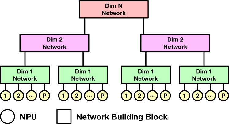
Figure 1: A generic overview of multi-dimensional networks. $P$ NPUs are first interconnected using Dim 1 network. Several of Dim 1 groups are then connected using Dim 2 network. In the end, a hierarchical $N$-dimensional topology is being created.

Communication. One of the biggest challenges with getting good performance out of these platforms is communication, as several previous studies have shown [16, 17, 26, 18, 25]. This is because, no matter what parallelization strategy is used, there is inevitable communication across NPUs to exchange gradients and/or activations.

Further, a high ratio of communication-to-computation in many DNN training workloads [17] makes them extremely difficult to scale, since communication becomes the bottleneck factor. Figure 2 shows the growth in the communication size of the most popular DNNs in recent years. High communication overhead diminishes the benefits of scaling. Moreover, this problem in fact gets exacerbated as compute becomes more efficient [5, 24].

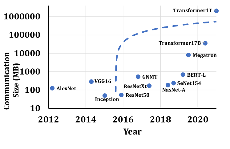
Figure 2: Communication size of recent models.

Designing Optimized Interconnects for Target Training Workloads. To reduce the communication overhead, training platforms should be equipped with efficient networks (interconnects) that are optimized for the set of target training workloads. Current distributed training platforms typically have 2D networks to connect all NPUs. On the first dimension (Dim 1), NPUs residing on the same server node are connected through high-BW interconnects. On the second dimension (Dim 2), the server nodes are connected together using network interface cards (NICs) [21, 6]. NICs are one of the most expensive components of the network, and compared to the Dim 1, have significantly lower BW (up to 12$\times$ BW difference [6]), hence, they easily become the bottleneck in terms of both performance of the training and cost of the network.

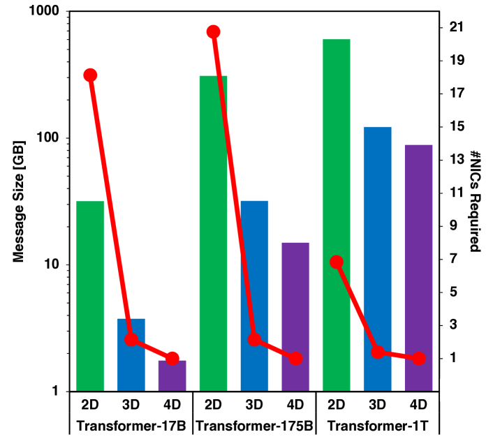
Figure 3: The amount of data sent-out on the last dimension (through NIC) of a 2D/3D/4D network through network interface (NIC), for the Transformer-17B, GPT-3 (Transformer-175B), Transformer-1T. The second y-axis shows the amount of NICs-per-NPU required for different networks if they were to have the same latency as the 4D topology for the last dimension. The details of the topology and workloads are explained in subsection VI-A.

Figure 3 shows the growing trend of increased traffic of NIC (last dimension) as the DNN model size increases. It also shows how adding intermediate network dimensions, and creating 3D and 4D topologies can reduce the NIC (last dimension) traffic. This is due to the nature of hierarchical collective communication algorithms (explained in detail in subsection III-B), which reduces the network message size as data goes to the next level of the network hierarchy, hence adding network dimensions further reduces data size once it reaches the last dimension NIC. Figure 3 also shows how many NICs-per-NPU are required for the 2D and 3D topologies to get to the equal last dimension performance of the 4D topology. This clearly shows how adding an intermediate network dimension can effectively reduce the last dimension traffic without the need to attach additional expensive NICs.

However, adding intermediate network dimensions have their own costs, as explained in detail in subsection III-C. When designing the interconnect, the BW distribution across different dimensions should be in a way that (i) effectively utilizes all network dimensions, and (ii) minimizes the overall training time. In this paper, we provide a framework that for a given target DNN workload, yields what is the best network configurations (in terms of the number of dimensions, BW distribution, etc.) that maximize performance, or performance-per-cost.

Overall, we make the following contributions:

• We motivate the need for designing more than 2-dimensional networks to better mitigate the communication overhead.

• We provide detailed analysis on how to overcome the challenges of the multi-dimensional networks and optimize their BW utilization and BW distribution.

• We establish a simulation methodology for the evaluation of the distributed training platform.

• We provide a framework that for a given target DNN workload, gives the optimized network configurations that maximize performance, or performance-per-cost.

II Background

II-A Collective Communication Patterns

Communication is the inevitable overhead to pay in distributed training workloads. The exact communication patterns each training workload requires depend on the parallelization strategy, and also the communication mechanism (e.g., parameter server vs. explicit NPU-to-NPU). When using the explicit NPU-to-NPU communication mechanism, All-Reduce is the most dominant pattern observed in distributed training [16]. For example, in the case of a data-parallel parallelization strategy, each NPU works on a subset of the global mini-batch in each iteration, thus, their calculated weight gradients must be globally reduced (i.e. All-Reduce) before updating the weights and starting the new training iteration.

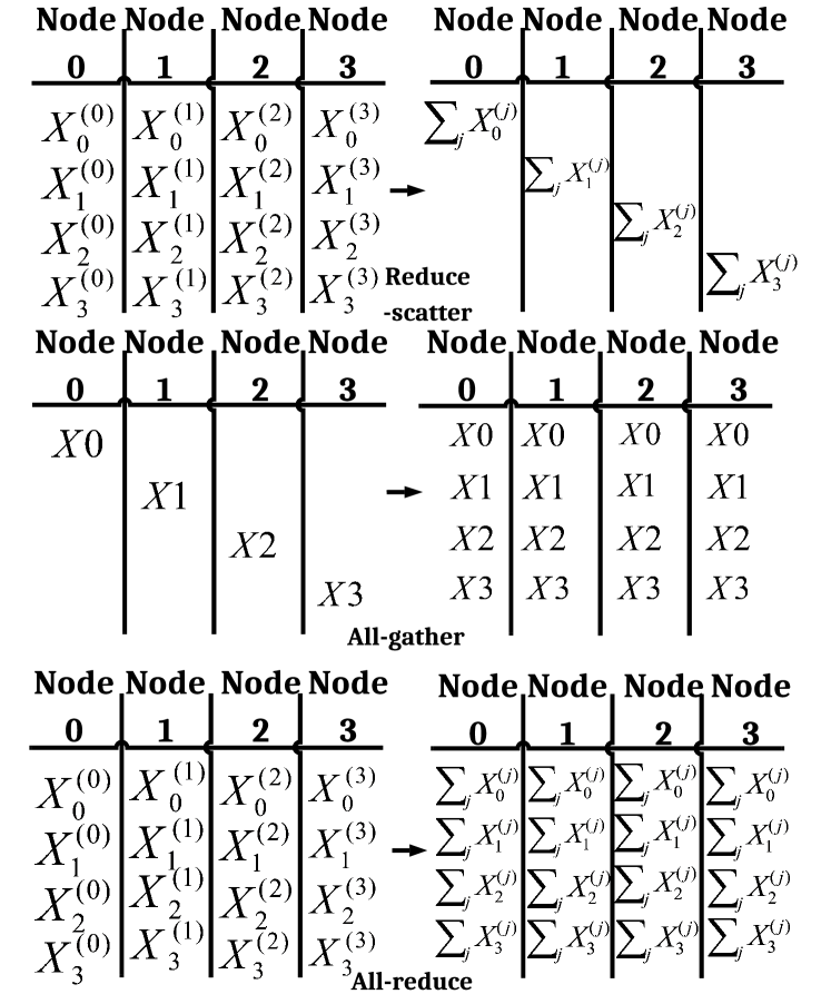
Figure 4: The Mathematical Implications of the Reduce-Scatter, All-Gather, and All-Reduce patterns executing on four NPUs. The left part shows the initial data on each communicating NPU before the collective operation. The right part shows data residing on each NPU after the completion of the collective operation.

All-Reduce can be broken into a Reduce-Scatter followed by an All-Gather communication patterns. Figure 4 shows the mathematical implications of these patterns performed on four NPUs. Reduce-Scatter performs reduction operation among initial data such that at the end, each NPU holds a portion of the globally reduced data. All-Gather, on the other hand, broadcasts data residing on each NPU to all other NPUs. Therefore, it is clear that when performing Reduce-Scatter/All-Gather on $P$ participating NPUs, the data size residing on each NPU shrinks/multiplies by $P\times$.

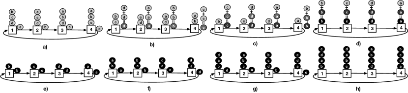
Figure 5: An example of the ring All-Reduce algorithm to perform the All-Reduce pattern. Steps a-d perform Reduce-Scatter pattern and steps e-g perform All-Gather pattern. Step h shows the final result.

II-B Basic Collective Communication Algorithms

Each of the collective communication patterns described in subsection II-A can be performed through different collective communication algorithms. For example, tree-based [22], ring-based [9], and halving-doubling [10] algorithms are proposed to realize All-Reduce pattern and are implemented in communication frameworks such as Intel oneCCL [14] or NVidia NCCL [20]. Figure 5 shows an example of the ring-based All-Reduce algorithm running on four NPUs. Assume the initial data residing on each NPU is $N$ and there are $P$ NPUs participating in the communication. In general, in a ring-based All-Reduce each NPU sends out $\frac{2N}{P}$ communication data to the network: $\frac{N}{P}$ during the Reduce-Scatter phase during $P$-1 steps, followed by another $\frac{N}{P}$ during the All-Gather during another $P$-1 steps. Figure 5 shows the special case when $P$=4. Moreover, the optimal algorithm is usually dependent on the physical topology and also the communication size [27].

For example, a physical ring topology connecting NPUs is a natural fit for ring-based algorithms. Communication size also plays a role in determining the best algorithm to be employed as previous methods showed [27]. Hence, communication libraries dynamically decide which algorithms to use based on the underlying physical topologies and communication sizes. Such basic collective algorithms provide a basis to design more complex and tuned algorithms that are optimized for multi-dimensional network topologies, as we describe next.

III Distributed Training on Multi-dimensional Hierarchical Networks and its Challenges

III-A Multi-dimensional Network

As described earlier in section I, the structure of multi-dimensional networks can be generalized as Figure 1. In the beginning, $P$ numbers of NPUs are interconnected by Dim 1 network. Several of such Dim 1 networks are then being linked by Dim 2 network. Likely, a number of Dim 2 networks can be connected using Dim 3 network. This process can reach up to Dim $N$, creating an $N$-dimensional network topology.

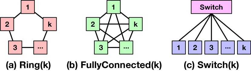
Figure 6: Building blocks of multi-dimensional hierarchical network utilized in this paper. Ring topology offers two connections to the adjacent NPUs whereas FullyConnected has all-to-all connectivity. Switch topology links all NPUs using a network switch.

In this work, there can be three types of network topologies that can be used as a network of each dimension: Ring, FullyConnected , and Switch. The shape of each network building block is depicted in Figure 6. Ring topology offers exactly two connections to the very adjacent NPUs. FullyConnected topology, on the other hand, provides all-to-all connectivity to all the other NPUs within the same dimension. This indicates all NPUs can reach all the other NPUs inside the same dimension in a single step. Switch topology uses an external network switch to connect all the NPUs under a dimension.

Physical multi-dimensional topologies can be realized by stacking up topology building blocks across multiple dimensions. Because of this very regular and rigid instantiation process, each multi-dimensional networks can be named and distinguished by listing the network building blocks and the number of NPUs of each dimension. Figure 7 gives five different examples of multi-dimensional hierarchical topologies. Looking at Figure 7(a), you can find that Dim 1 consists of 4 NPUs connected by FullyConnected, then two of such networks connected using Ring to create Dim 2. Therefore, Figure 7(a) can be named as FC(4)_Ring(2). Figure 7(b), unlike Figure 7(a), is utilizing Ring in Dim 1. Therefore, Figure 7(b) is named as Ring(4)_FC(2). Note that for topologies with 2 NPUs, Ring and FullyConnected have the same connectivity. For example, Figure 7(a) could be named as FC(2)_FC(2) or Figure 7(b) can be called as Ring(4)_Ring(2). Following the same notion, Figure 7(c) depicts a Switch(3)_FC(2) (or Switch(3)_Ring(2)) network. Figure 7(d) is a 3D topology, of which all dimensions consist Ring. This can be named as Ring(4)_Ring(2)_Ring(2), and is effectively modeling a 3D $4\times 2\times 2$ torus network. Finally, Figure 7(e) altered Dim 1 of Figure 7(d) by using FullyConnected instead, thereby instantiating a FC(4)_Ring(2)_Ring(2) hierarchical network.

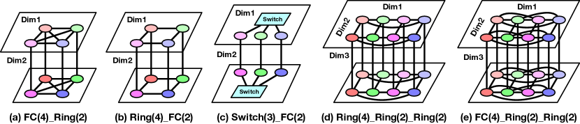
Figure 7: Examples of multi-dimensional topologies and their names used in this paper. (a)-(c) two-dimensional networks (d)-(e) three-dimensional networks.

III-B Hierarchical Collective Communication Algorithms

In subsection II-B, we have stated basic collective communication algorithms, such as ring-based, tree-based, or halving-doubling algorithms. These basic collective communication algorithms are not a good fit to be directly utilized on multi-dimensional hierarchical topologies. It’s because some NPU pairs required to transmit payloads in the basic collective communication scheme would not be efficiently connected in multi-dimensional networks. This not only creates huge network congestion but also increments collective communication time because of the very synchronous nature of basic collective communication algorithms. Therefore, a multi-rail hierarchical collective algorithm, which is aware of the structure of hierarchical topologies, is proposed to fully exploit different topologies and configurations of dimensions.

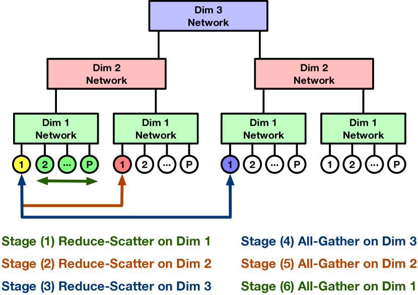
Figure 8: Running hierarchical All-Reduce on a 3-dimensional topology. First, Reduce-Scatter collective is run in ascending dimension order. Then, All-Gather is performed in descending dimension order. In total, this takes 6 stages of running collectives within each dimension.

In order to run an All-Reduce collective on a $N$ dimensional network,

• Run Reduce-Scatter on Dim 1. Then, run Reduce-Scatter on Dim 2. This Reduce-Scatter jobs in ascending order continue all the way up to Dim $N$ (in total $N$ Reduce-Scatter stages).

• Perform All-Gather on Dim $N$. Then, execute All-Gather in Dim $N-1$. This All-Gather stage continues, in descending order, from Dim $N$ down to Dim 1 (in total $N$ All-Gather stages).

In total, hierarchical All-Reduce collective communication algorithm takes $2N$ stages of Reduce-Scatter and All-Gather combined. Within each stage, each dimension utilizes basic collective communication algorithms shown in subsection II-B to execute Reduce-Scatter and All-Gather.

In order not to create any congestion on each network dimension and to maximize performance, the best basic collective algorithm is chosen and run depending on the topology of each network dimension. This is named a topology-aware collective communication algorithm. Topology-aware collective communication algorithms are proven not to incur any congestion into the network. The corresponding topology-aware collective communication algorithms of the network building blocks used in this paper are listed in Table I.

TABLE I: Network building blocks and their corresponding topology-aware All-Reduce collective communication algorithms, which don’t create any congestion into the network.

Topology	Topology-aware Collective
Ring	Ring
FullyConnected	Direct
Switch	HalvingDoubling

III-C Challenges with Hierarchical Collective Communication Algorithms on Distributed Training Workloads

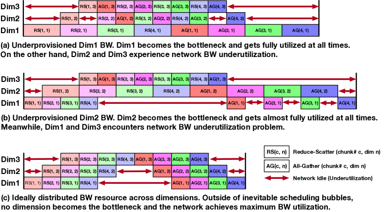
Figure 9: Running an All-reduce collective with 4 chunks, on three different 3-dimensional topologies with different BW resource allocation.

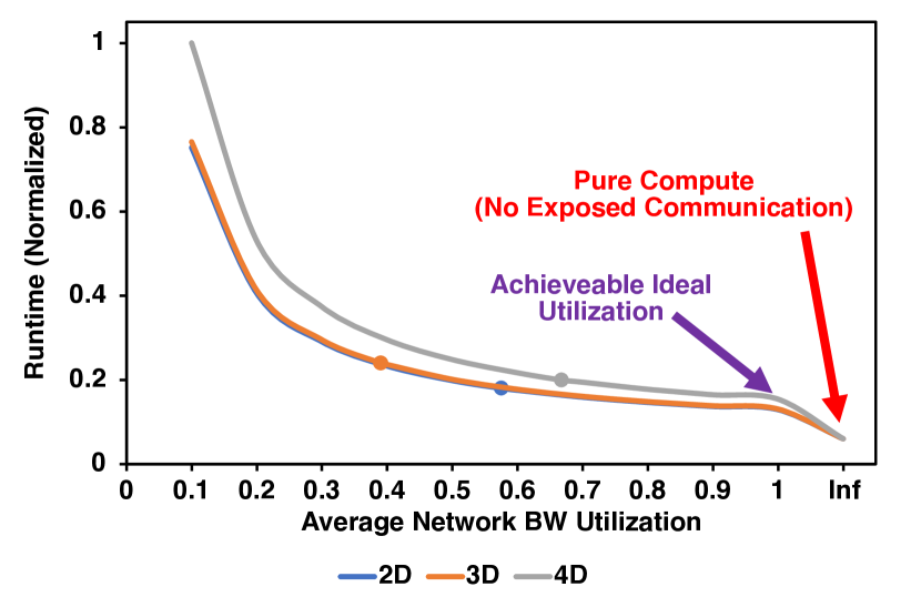
Figure 10: The normalized end-to-end training time of Transformer-1T on 2D, 3D, and 4D topologies with 300GBps/NPU aggregated BW resource. Training time increases as we increase the number of network dimensions. Average network BW utilization was around 39.02-66.74% when the BW resource is distributed equally among dimensions. We can achieve 1.83$\times$ maximum speedup if we can reach 100% of the average BW utilization.

Figure 8 is an example hierarchical All-Reduce collective communication on a 3-dimensional network. Following the hierarchical All-Reduce algorithm explained in subsection III-B, the first stage is performing Reduce-Scatter on Dim 1. Assuming $P$ NPUs exist in Dim 1, this Reduce-Scatter partially reduces the message size by $P\times$, as shown in subsection II-B. The next step is to execute Reduce-Scatter on Dim 2, further reducing the payload size for Dim 3. Therefore, during the Reduce-Scatter phase, message sizes flowing alongside dimensions monotonically decrease as reaching higher network dimension.

Once Reduce-Scatter phase is done, All-Gather phase begins starting Dim 3. Distributing message across NPUs, All-Gather increases payload size of Dim 2 All-Gather. Dim 2 All-Gather also expands message size for Dim 1 All-Gather. As a consequence, during the All-Gather stage, payload sizes increment as we reach lower dimensions.

Single collective communication can be split into a number of chunks and be run in a pipelined manner, to utilize all the network dimensions simultaneously. Figure 9 is depicting such case by running an All-Reduce collective communication using 4 chunks. Figure 9(a) is a configuration where very limited network bandwidth resource is allocated to Dim 1. In this case, executing collective chunks on Dim 1 becomes the bottleneck of the entire network. As a consequence, Dim 1 gets utilized 100% of the time, whereas Dim 2 and Dim 3 experience severe underutilization. Figure 9(b) shows another analogous case where Dim 2 has underprovisioned bandwidth. In this configuration, Dim 2 becomes the critical dimension and both Dim 1 and Dim 3 suffer high network underutilization. Figure 9(c) paints the ideal case where bandwidth resources are properly distributed across all dimensions. This configuration minimizes the network underutilization and finishes the collective communication in the shortest time. Therefore, to fully leverage given network resources and train a network with the maximum possible efficiency, the need for intelligent bandwidth allocation across network dimensions is necessitated.

Figure 10 is showing Transformer-1T training time on 300GBps/NPU networks with various dimensions. With the baseline configuration (explained in subsection IV-A) where all the dimensions have equal bandwidth, average network bandwidth utilization were 57.53%, 39.02%, 66.74% for 2D, 3D, 4D networks, respectively. By maximizing the network bandwidth utilization, we can theoretically achieve the training speedup of 1.39$\times$, 1.83$\times$, and 1.29$\times$, respectively. To re-iterate, designing an intelligent network bandwidth allocation scheme is pivotal.

IV Bandwidth Allocation Scheme to Fully Utilize Network Bandwidth

Aforementioned in subsection III-C, assigning network bandwidth resources without deep consideration could lead to severe network underutilization. Consequently, this can yield longer end-to-end training time due to network communication inefficiency. Therefore, optimized distribution of bandwidth budget across dimensions is necessitated to facilitate the full efficiency of the network.

In this section, we explain three different bandwidth distribution schemes: EqualBW, MessageBW, and SmartBW. Assuming an NPU has $B$ bandwidth resource, each scheme targets to distribute it across dimensions with different patterns.

Notations used in this section is defined as follows. Per each NPU:

$$B:\text{Bandwidth budget.}$$

$$N:\text{Number of dimensions of the network.}$$

$$M(k):\text{Message size transmitted through dimension }k.$$

$$BW(k):\text{Bandwidth allocated to dimension }k.$$

IV-A EqualBW

The baseline allocation, EqualBW, distributes the given bandwidth resource equally across dimensions without using any additional metadata.

$$BW(k)=\frac{B}{N}$$ (1)

In this paper, we regard EqualBW as a baseline bandwidth allocation scheme for given network topology. EqualBW does not require any metadata for bandwidth allocation and thereby workload-agnostic and network-dependent.

IV-B MessageBW

Bandwidth can be distributed proportionally to the message size transmitted through each dimension. This scheme is named MessageBW, as the bandwidth of a dimension is decided solely by message size.

$$BW(k)=\frac{M(k)}{\sum_{i=1}^{N}M(i)}\times B$$ (2)

IV-C SmartBW

MessageBW defined in subsection IV-B yields the optimal performance when the transmissions of all dimensions run concurrently in parallel. When the workload is parallelized in either pure DP or MP manner, this condition is satisfied and MessageBW yields the best performance.

However, one should note that MP and DP communication may not run concurrently and rather get executed sequentially. Several models utilize a hybrid parallelization scheme, utilizing both MP and DP communication. In this setup, several dimensions (usually lower-level dimensions) run MP communication while some other dimensions are responsible for DP collectives. Figure 11 explains such cases on a $2\times 8\times 8\times 8$ topology. Figure 11(a) is the case when the workload is exploiting the hybrid scheme with MP-16 and DP-64. In this setup, Dim 1 and Dim 2 run MP communication first. After MP communication is finalized, the last two dimensions, Dim 3 and Dim 4 run DP communication. One can instantaneously see that the four dimensions never work simultaneously at any given time. Figure 11(b) is explaining a more complex case, where the workload is now MP-32 and DP-32. For MP communication, in this case, MP spans across Dim 1, Dim 2, and Dim 3, as MP requires 32 NPUs. After MP transmission, DP communication is processed using Dim 3 and Dim 4. In this setup, Dim 3 is shared by both MP and DP and transmits both MP and DP messages. Please note that MP and DP messages via Dim 3 are not processed concurrently, though. It is plausible that up to one dimension can be leveraged by both MP and DP. We will call this dimension a shared dim.

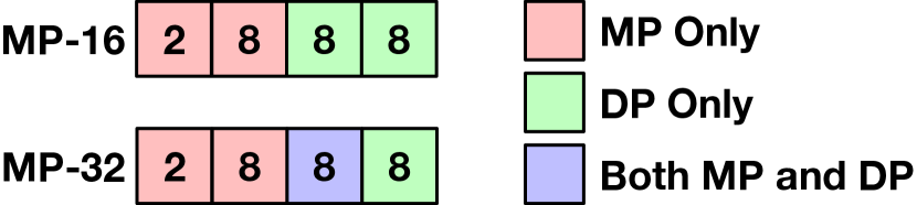
Figure 11: Running MP-16 and MP-32 workloads on 4D (2$\times$8$\times$8$\times$8) topology. For MP-16 workloads, Dim 1–2 run only MP communication, and Dim 3–4 only run DP communication. For MP-32 workloads, Dim 1–2 runs only MP, Dim 4 runs only DP, but Dim 3 is shared for both MP and DP communications.

Let’s first solve the case without a shared dimension. Let bandwidth assigned to MP dims are $BW(MP)$, and likely $BW(DP)$ assigned to DP dims. Similarly, the total message size of MP and DP communications can be expressed as $M(MP)$ and $M(DP)$, respectively. Network communication time for one training iteration can be expressed as follows:

$$\frac{M(MP)}{BW(MP)}+\frac{M(DP)}{BW(DP)}$$

as MP and DP are running serially.

The objective is to distribute the bandwidth resource such that the network minimizes the training time.

$$\operatorname*{argmin}_{BW(MP),BW(DP)}\left(\frac{M(MP)}{BW(MP)}+\frac{M(DP)}{BW(DP)}\right)$$ (3)

$$\text{s.t. }BW(MP)+BW(DP)=B$$ (4)

Equation 3 is an ILP problem with a condition of Equation 4, and this solves as

$$BW(MP)=\frac{\sqrt{M(MP)}}{\sqrt{M(MP)}+\sqrt{M(DP)}}\times B$$ (5)

$$BW(DP)=\frac{\sqrt{M(DP)}}{\sqrt{M(MP)}+\sqrt{M(DP)}}\times B$$ (6)

Equation 5 and Equation 6 show that MP and DP dimensions should distribute the total bandwidth resource $B$ by the square root of their message sizes. Then, as dimensions within MP and DP runs concurrently, we can distribute $BW(MP)$ and $BW(DP)$ across dimensions proportionally to the message size.

Now, for the case with a shared dimension, still the objective function (Equation 3) still remains but the condition changes. Let the ratio of MP and DP message size processed by the shared dim be $r_{MP}$ and $r_{DP}$, respectively.

$$r_{MP}=\frac{M(MP\_s)}{M(MP)}$$

$$r_{DP}=\frac{M(DP\_s)}{M(DP)}$$

Then, the bandwidth resource allocated for this shared dimension, in MP and DP’s perspective, is calculated as follows.

$$BW(MP\_S)=r_{MP}\times BW(MP)$$

$$BW(DP\_S)=r_{DP}\times BW(DP)$$

Likely, bandwidths for non-shared MP and DP dimensions can be calculated as below.

$$BW(MP\_NS)=(1-r_{MP})\times BW(MP)$$

$$BW(DP\_NS)=(1-r_{DP})\times BW(DP)$$

The shared dimension bandwidth should be maximum of these two, to support both MP and DP in a maximum efficient manner.

$$BW(S)=\max\left(BW(MP\_S),BW(DP\_S)\right)$$

Bandwidth resources allocated for non-shared MP, non-shared DP, and shared dim, should be equal to the total bandwidth budget when aggregated. Therefore:

$$B=BW(MP\_NS)+BW(DP\_NS)+BW(S)$$ (7)

Now, we can solve for the same ILP problem (Equation 3) under the newly computed condition (Equation 7). This ILP problem has a closed-form solution, however, we omitted the result here for the sake of the space.

This scheme is named SmartBW because this scheme leverages workload metadata extensively and theoretically minimizes the end-to-end communication time.

V Framework for Training Performance and Network Cost Estimation

We use analytical-equation-based simulations to estimate the end-to-end training time performance and network cost. This scheme could estimate performance and cost within remote error margins in a very swift manner. The simulation framework is open-sourced and readily available.

V-A Analytical Framework to Simulate DL Training on Multi-dimensional Topologies

We used ASTRA-sim [24] as the frontend to simulate distributed training. ASTRA-sim frontend simulates the distributed training workload, which in turn generates a series of send and receive requests among different sets of NPUs with corresponding callback functions.

The analytical-equation-based framework captures these requests and simulates the transmission based on a simple network latency estimation equation. The framework maintains its own event queue. Using the analytical estimation, the framework schedules the callback function into its event queue, so that the ASTRA-sim frontend can capture the analytical network estimation and keep simulating distributed training.

$$\text{Time}=(\text{LinkLatency}\times\text{Hops})+\frac{\text{MessageSize}}{\text{LinkBandwidth}}$$ (8)

The equation to compute the communication time between two NPUs is shown in Equation 8. It exploits the fundamental abstraction that network communication time is a combination of link delay and serialization delay. This, respectively, consists of link latency, hops between NPUs, message size, and link bandwidth.

V-B Cost Model to Estimate Network Price

TABLE II: Unit cost of different network components.

Component	Unit	Unit Price ($)
Link	1 GB/s	2
NIC	1 GB/s	48
Switch	1 radix $\cdot$ GB/s	24

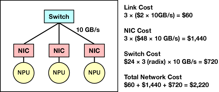
Figure 12: Example cost modeling. This network topology consists of 3 NPUs connected via a global switch. Therefore, the cost model evaluates the cost of 3 links, 3 NICs, and 1 switch with the given network configuration parameters.

A network consists of multiple different components, and each component has different cost estimations. The cost model we used to estimate network price is represented in Table II. As Table II suggests, each network can consist of three different components: Link, NIC, and Switch. NIC is used whenever it’s required to interconnect an NPU with a switch. Each link costs $2 per 1GB/s. Likely, each NIC costs $48 per 1GB/s, and a switch costs $24 per 1 radix$\cdot$GB/s.

An example cost estimation for a given network is explained in Figure 12. This example network uses all three network components. There is one switch of radix 3, three NICs to connect NPUs and the switch, and three 10GB/s links. As shown in Table II, each 10GB/s link costs $20 and there are three such links, thereby retrieving the total link cost of $60. The same applies to NICs and the switch. In the end, the network cost of Figure 12 is calculated as $2,220.

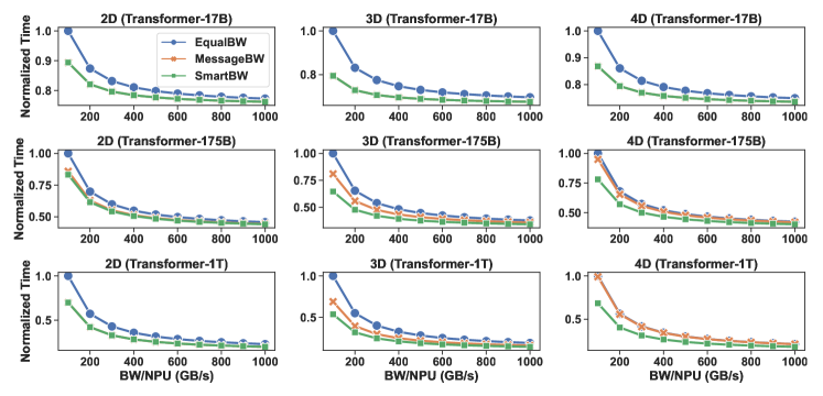
Figure 13: End-to-end training time. Training times are normalized by EqualBW (100GBps/NPU) of each network configuration.

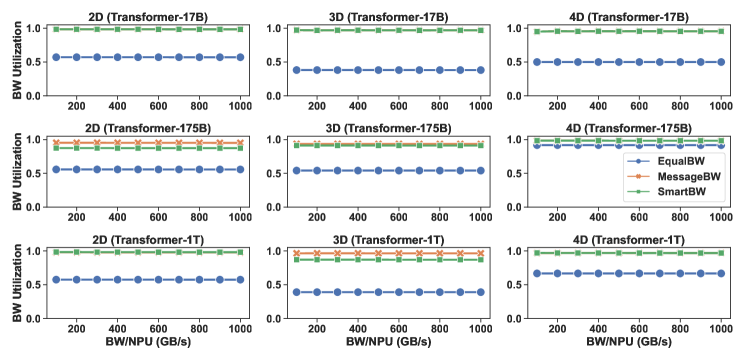
Figure 14: Average bandwidth utilization.

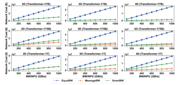
Figure 15: Cost of each network estimated by the analytical cost model.

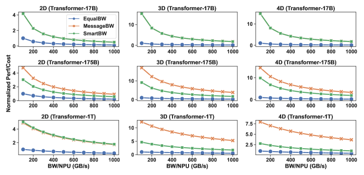
Figure 16: Network training performance per cost. Results are normalized by EqualBW (100GBps/NPU) of each network configuration.

VI Results

VI-A Experimental Setup

In this paper, we simulate three different networks, all equipped with 1,024 NPUs but consist of a various number of network dimensions. Table III shows physical network setups used in this paper for 2D, 3D, and 4D networks. We used Ring_Switch for 2D networks with size $8\times 128$. Likely, 3D and 4D networks are equipped with Ring_FullyConnected_Switch with size $8\times 8\times 16$ and Ring_FullyConnected_Ring_Switch with size $2\times 8\times 8\times 8$, respectively.

TABLE III: Physical network topologies used for analysis.

Dim	Shape	Size	NPUs
2D	Ring_Switch	$8\times 128$	1,024
3D	Ring_FC_Switch	$8\times 8\times 16$	1,024
4D	Ring_FC_Ring_Switch	$2\times 8\times 8\times 8$	1,024

Table IV lists the workloads and their characteristics used in this paper. We used three different transformer-based workloads: Transformer-17B, GPT-3, and Transformer-1T. Transformer-17B utilizes pure data-parallel (DP-1024). GPT-3 utilizes a hybrid scheme, with MP-16 and DP-64. Transformer-1T also leverages hybrid parallelization with MP-128 and DP-8. Compute times are modeled assuming each NPU compute speed is 234 TFLOPS. The parallelization schemes of each workload shown in Table IV are deduced with ZeRO phase-2 optimizers [23].

TABLE IV: Workloads and their characteristics used for analysis.

Workload	Params (B)	MP Size	DP Size
Transformer-17B	17	-	1,024
GPT-3	175	16	64
Transformer-1T	1,024	128	8

VI-B Performance

In this section, we provide our analysis of how different BW allocation schemes affect the overall end-to-end performance of training workloads. Here, the goal is to explore the best scheme that minimizes the training time. Figure 13 shows the performance comparison of EqualBW, MessageBW, and SmartBW for Transformer-17B, GPT-3, and Transformer-1T, when running on Ring_Switch, Ring_FullyConnected_Switch, Ring_FullyConnected_Ring_Switch topologies. As Figure 13 shows, increasing the total aggregated BW reduces the overall training time, but the slope of performance improvement decreases as BW increases. This is due to the fact that by increasing BW, communication overhead is reduced, and hence, compute overhead starts to become the dominant factor, resulting in diminishing performance improvement as BW increases. Also, note that the improvement gain also depends on the initial communication-to-compute overheads of the workloads running a given topology. This means that those workload/topology configurations with higher communication-to-compute overhead gain more performance improvement as the aggregated BW increases.

When comparing different BW allocation schemes, SmartBW always gives the best performance across all workload/topology/BW configurations. On average, MessageBW and SmartBW achieve 1.10$\times$ (1.45$\times$ max) and 1.17$\times$ (1.86$\times$ max) better performance when compared to the naive EqualBW configuration, respectively.

For better understanding regarding the source of benefit, Figure 14 shows the corresponding average network BW utilization for each configuration. According to Figure 14, on average, EqualBW, MessageBW, SmartBW reach to the BW utilization of 56.67%, 96.59%, and 94.46%, respectively. An interesting point is that for configurations with a shared network dimension between MP and DP, SmartBW average utilization is slightly lower than MessageBW, while according to Figure 13, SmartBW has the best performance. The reason is that the communication latency arises from two components of MP and DP communication overheads. When having the shared network dimension, the shared dimension BW may be fully utilized by MP/DP while not completely used by DP/MP communication. However, the overall communication latency depends on the summation of MP+DP overheads, which in the case of SmartBW gives the lowest overhead.

VI-C Performance Per Cost

In this section, we set the goal to be the best performance to cost ratio. Figure 15 shows how network cost increases as a function of total aggregated BW for different configurations. In general EqualBW has the highest cost since such BW allocation requires considerable BW on the last dim (the NIC dim) which is very costly. Moreover, the SmartBW allocation is more costly compared to MessageBW, again because SmartBW requires more BW on the last dim. On average, SmartBW and EqualBW cost is 7.77$\times$ (13.82$\times$ max) and 1.65$\times$ (4.13$\times$ max) when compared to the MessageBW cost, respectively.

Figure 16 shows the performance-per-cost for different configurations. As indicated in Figure 16, the performance-per-cost drops as total BW increases. This because of the reduced role of communication in determining training time as BW increases (as discussed in subsection VI-B). In terms of performance-per-cost, MessageBW works best, while SmartBW is the second to best and EqualBW is the worst. On average, the performance-per-cost of MessageBW and SmartBW is 8.52$\times$ (17.02$\times$ max) and 5.51$\times$ (15.37$\times$ max) higher than EqualBW, respectively.

Figure 13 and Figure 16 clearly show how setting different target goals affects the best network BW allocation choices in the design time of the training system platforms. These figures also show how different workloads get different benefits from such BW optimization schemes. This is one of the major contributions of the paper, that tries to provide a systematic way of thinking about network architecture during design time, with the aim to maximize the goal for a set of workloads.

VII Conclusion

In this paper, we provided a systematic way to determine the best multi-dimensional hierarchical network configuration for any target training workload. We started by motivating the fact that adding more intermediate network dimensions helps reduce the communication overhead and excessive NIC required for the scale-out network. We then analyzed the challenges of the multi-dimensional networks, mainly how BW should be distributed across to maximize the BW utilization and minimize the overall communication time. We then provided a simulation infrastructure to evaluate different training platforms. Finally, we provided a framework that determines the best network configuration for any set of target training workloads.

References

- [1] “Cloud TPU,” https://cloud.google.com/tpu.
- [2] “Fully Sharded Data Parallel: faster AI training with fewer GPUs,” https://engineering.fb.com/2021/07/15/open-source/fsdp.
- [3] “Google Open-Sources Trillion-Parameter AI Language Model Switch Transformer,” https://www.infoq.com/news/2021/02/google-trillion-parameter-ai/.
- [4] “Habana,” https://habana.ai.
- [5] “NVIDIA A100 TENSOR CORE GPU,” https://www.nvidia.com/en-us/data-center/a100/.
- [6] “NVIDIA DGX SuperPOD: Instant Infrastructure for AI Leadership,” https://resources.nvidia.com/en-us-auto-datacenter/nvpod-superpod-wp-09.
- [7] D. Amodei and D. Hernandez, “Ai and compute,” 2018. [Online]. Available: https://openai.com/blog/ai-and-compute/
- [8] T. B. Brown, B. Mann, N. Ryder, M. Subbiah, J. Kaplan, P. Dhariwal, A. Neelakantan, P. Shyam, G. Sastry, A. Askell, S. Agarwal, A. Herbert-Voss, G. Krueger, T. Henighan, R. Child, A. Ramesh, D. M. Ziegler, J. Wu, C. Winter, C. Hesse, M. Chen, E. Sigler, M. Litwin, S. Gray, B. Chess, J. Clark, C. Berner, S. McCandlish, A. Radford, I. Sutskever, and D. Amodei, “Language models are few-shot learners,” CoRR, vol. abs/2005.14165, 2020. [Online]. Available: https://arxiv.org/abs/2005.14165
- [9] E. Chan, R. van de Geijn, W. Gropp, and R. Thakur, “Collective communication on architectures that support simultaneous communication over multiple links,” in Proceedings of the Eleventh ACM SIGPLAN Symposium on Principles and Practice of Parallel Programming, ser. PPoPP ’06. New York, NY, USA: ACM, 2006, pp. 2–11. [Online]. Available: http://doi.acm.org/10.1145/1122971.1122975
- [10] J. Dong, Z. Cao, T. Zhang, J. Ye, S. Wang, F. Feng, L. Zhao, X. Liu, L. Song, L. Peng, Y. Guo, X. Jiang, L. Tang, Y. Du, Y. Zhang, P. Pan, and Y. Xie, “Eflops: Algorithm and system co-design for a high performance distributed training platform,” in 2020 IEEE International Symposium on High Performance Computer Architecture (HPCA), 2020, pp. 610–622.
- [11] A. Harlap, D. Narayanan, A. Phanishayee, V. Seshadri, N. Devanur, G. Ganger, and P. Gibbons, “Pipedream: Fast and efficient pipeline parallel dnn training,” 2018.
- [12] K. He, X. Zhang, S. Ren, and J. Sun, “Deep residual learning for image recognition,” CoRR, vol. abs/1512.03385, 2015. [Online]. Available: http://arxiv.org/abs/1512.03385
- [13] Y. Huang, Y. Cheng, A. Bapna, O. Firat, M. X. Chen, D. Chen, H. Lee, J. Ngiam, Q. V. Le, Y. Wu, and Z. Chen, “Gpipe: Efficient training of giant neural networks using pipeline parallelism,” 2019.
- [14] Intel, “Intel oneAPI Collective Communications Library,” 2020. [Online]. Available: https://software.intel.com/content/www/us/en/develop/tools/oneapi/components/oneccl.html
- [15] X. Jia, S. Song, W. He, Y. Wang, H. Rong, F. Zhou, L. Xie, Z. Guo, Y. Yang, L. Yu, T. Chen, G. Hu, S. Shi, and X. Chu, “Highly scalable deep learning training system with mixed-precision: Training imagenet in four minutes,” 2018.
- [16] B. Klenk, N. Jiang, G. Thorson, and L. Dennison, “An in-network architecture for accelerating shared-memory multiprocessor collectives,” in 2020 ACM/IEEE 47th Annual International Symposium on Computer Architecture (ISCA), 2020, pp. 996–1009.
- [17] Y. Li, I.-J. Liu, Y. Yuan, D. Chen, A. Schwing, and J. Huang, “Accelerating distributed reinforcement learning with in-switch computing,” in Proceedings of the 46th International Symposium on Computer Architecture, ser. ISCA ’19. New York, NY, USA: Association for Computing Machinery, 2019, p. 279–291. [Online]. Available: https://doi.org/10.1145/3307650.3322259
- [18] H. Mikami, H. Suganuma, P. U-chupala, Y. Tanaka, and Y. Kageyama, “Imagenet/resnet-50 training in 224 seconds,” 11 2018.
- [19] M. Naumov, D. Mudigere, H. M. Shi, J. Huang, N. Sundaraman, J. Park, X. Wang, U. Gupta, C. Wu, A. G. Azzolini, D. Dzhulgakov, A. Mallevich, I. Cherniavskii, Y. Lu, R. Krishnamoorthi, A. Yu, V. Kondratenko, S. Pereira, X. Chen, W. Chen, V. Rao, B. Jia, L. Xiong, and M. Smelyanskiy, “Deep learning recommendation model for personalization and recommendation systems,” CoRR, vol. abs/1906.00091, 2019. [Online]. Available: http://arxiv.org/abs/1906.00091
- [20] NVIDIA, “NVIDIA Collective Communication Library (NCCL),” 2017. [Online]. Available: https://developer.nvidia.com/nccl
- [21] NVIDIA, “NVIDIA DGX-2,” 2019. [Online]. Available: https://www.nvidia.com/en-us/data-center/dgx-2/
- [22] P. Patarasuk and X. Yuan, “Bandwidth optimal all-reduce algorithms for clusters of workstations,” J. Parallel Distrib. Comput., vol. 69, no. 2, pp. 117–124, Feb. 2009. [Online]. Available: http://dx.doi.org/10.1016/j.jpdc.2008.09.002
- [23] S. Rajbhandari, J. Rasley, O. Ruwase, and Y. He, “Zero: Memory optimizations toward training trillion parameter models,” 2020. [Online]. Available: https://arxiv.org/abs/1910.02054
- [24] S. Rashidi, S. Sridharan, S. Srinivasan, and T. Krishna, “Astra-sim: Enabling sw/hw co-design exploration for distributed dl training platforms,” in 2020 IEEE International Symposium on Performance Analysis of Systems and Software (ISPASS), 2020, pp. 81–92.
- [25] S. Rashidi, S. Sridharan, S. Srinivasan, M. Denton, A. Suresh, J. Nie, and T. Krishna, “Enabling compute-communication overlap in distributed training platforms,” in Procedings of 48th International Symposium on Computer Architecture (ISCA), 2021.
- [26] A. Sapio, M. Canini, C. Ho, J. Nelson, P. Kalnis, C. Kim, A. Krishnamurthy, M. Moshref, D. R. K. Ports, and P. Richtárik, “Scaling distributed machine learning with in-network aggregation,” CoRR, vol. abs/1903.06701, 2019. [Online]. Available: http://arxiv.org/abs/1903.06701
- [27] R. Thakur, R. Rabenseifner, and W. Gropp, “Optimization of collective communication operations in mpich,” Int. J. High Perform. Comput. Appl., vol. 19, no. 1, pp. 49–66, Feb. 2005. [Online]. Available: http://dx.doi.org/10.1177/1094342005051521
- [28] I. Thangakrishnan, D. Cavdar, C. Karakus, P. Ghai, Y. Selivonchyk, and C. Pruce, Herring: Rethinking the Parameter Server at Scale for the Cloud. IEEE Press, 2020.
- [29] A. Vaswani, N. Shazeer, N. Parmar, J. Uszkoreit, L. Jones, A. N. Gomez, L. Kaiser, and I. Polosukhin, “Attention is all you need,” CoRR, vol. abs/1706.03762, 2017. [Online]. Available: http://arxiv.org/abs/1706.03762