Safe Policy Learning through Extrapolation: Application to Pre-trial Risk Assessment††thanks: We acknowledge the partial support from Cisco Systems, Inc. (CG# 2370386), National Science Foundation (SES–-2051196), Sloan Foundation (Economics Program; 2020–13946), and Arnold Ventures. We thank anonymous reviewers of the IQSS’s Alexander and Diviya Magaro Peer Pre-Review Program for useful feedback.
This draft: )
Abstract
Algorithmic recommendations and decisions have become ubiquitous in today’s society. Many of these and other data-driven policies, especially in the realm of public policy, are based on known, deterministic rules to ensure their transparency and interpretability. For example, algorithmic pre-trial risk assessments, which serve as our motivating application, provide relatively simple, deterministic classification scores and recommendations to help judges make release decisions. How can we use the data based on existing deterministic policies to learn new and better policies? Unfortunately, prior methods for policy learning are not applicable because they require existing policies to be stochastic rather than deterministic. We develop a robust optimization approach that partially identifies the expected utility of a policy, and then finds an optimal policy by minimizing the worst-case regret. The resulting policy is conservative but has a statistical safety guarantee, allowing the policy-maker to limit the probability of producing a worse outcome than the existing policy. We extend this approach to common and important settings where humans make decisions with the aid of algorithmic recommendations. Lastly, we apply the proposed methodology to a unique field experiment on pre-trial risk assessment instruments. We derive new classification and recommendation rules that retain the transparency and interpretability of the existing instrument while potentially leading to better overall outcomes at a lower cost.
Keywords: algorithm-assisted decision-making; observational studies; optimal policy learning; randomized experiments; robust optimization
1 Introduction
Algorithmic recommendations and decisions are ubiquitous in our daily lives, ranging from online shopping to job interview screening. Many of these algorithm-assisted, or simply data-driven, policies are also used for highly consequential decisions including those in the criminal justice system, social policy, and medical care. One important feature of such policies is that they are often based on known, deterministic rules. This is because transparency and interpretability are required to ensure accountability especially when used for public policy-making. Examples include eligibility requirements for government programs (e.g., Canadian permanent residency program; Supplemental Nutrition Assistance Program or SNAP, Center on Budget and Policy Priorities, 2017) and recommendations for medical treatments (e.g., MELD score for liver transplantation, Kamath et al., 2001).
The large amounts of data collected after implementing such deterministic policies provide an opportunity to learn new policies that improve on the status quo. Unfortunately, prior approaches for policy learning are not applicable because they require existing policies to be stochastic, typically relying on inverse probability-of-treatment weighting. To address this challenge, we propose a robust optimization approach that finds an improved policy without inadvertently leading to worse outcomes. To do this, we partially identify the expected utility of a policy by calculating all potential values consistent with the observed data, and find the policy that maximizes the expected utility in the worst case. The resulting policy is conservative but has a statistical safety guarantee, allowing the policy-maker to limit the probability for yielding a worse outcome than the existing policy.
We formally characterize the gap between this safe policy and the infeasible oracle policy as a function of restrictions imposed on the class of outcome models as well as on the class of policies. After developing the theoretical properties of the safe policy in the population, we show how to empirically construct the safe policy from the data at hand and analyze its statistical properties. We then provide details about the implementation in several representative cases. We also consider two extensions that directly address the common settings, including our application, where a deterministic policy is experimentally evaluated against a “null policy,” and humans ultimately make decisions with the aid of algorithmic recommendation. The availability of experimental data weakens the required assumptions while human decisions add extra uncertainty.
Our motivating empirical application is the use of pre-trial risk assessment instruments in the American criminal justice system. The goal of a pre-trial risk instrument is to aid judges in deciding which arrestees should be released pending disposition of any criminal charges. Algorithmic recommendations have long been used in many jurisdictions to help judges make release and sentencing decisions. A well-known example is the COMPAS score, which has ignited controversy (e.g., Angwin et al., 2016; Dieterich et al., 2016; Rudin et al., 2020). We analyze a particular pre-trial risk assessment instrument used in Dane county, Wisconsin, that is different from the COMPAS score. This risk assessment instrument assigns integer classification scores to arrestees according to the risk that they will engage in risky behavior. It then aggregates these scores according to a deterministic function and provides an overall release recommendation to the judge. Our goal is to learn new algorithmic scoring and recommendation rules that can lead to better overall outcomes while retaining the transparency of the existing instrument. Importantly, we focus on changing the algorithmic policies, which we can intervene on, rather than judge’s decisions, which we cannot.
We apply the proposed methodology to the data from a unique field experiment on pre-trial risk assessment (Greiner et al., 2020; Imai et al., 2020). Our analysis focuses on two key components of the instrument: (i) classifying the risk of a new violent criminal activity (NVCA) and (ii) recommending cash bail or a signature bond for release. We show how different restrictions on the outcome model, while maintaining the same policy class as the existing one, change the ability to learn new safe policies. We find that if the cost of an NVCA is sufficiently low, we can safely improve upon the existing risk assessment scoring rule by classifying arrestees as lower risk. However, when the cost of an NVCA is high, the resulting safe policy falls back on the existing scoring rule. For the overall recommendation, we find that noise is too large to improve upon the existing recommendation rules with a reasonable level of certainty, so the safe policy retains the status quo.
Related work.
Recently, there has been much interest in finding population optimal policies from randomized trials and observational studies. These methods typically use either inverse probability weighting (IPW) (e.g. Beygelzimer and Langford, 2009; Qian and Murphy, 2011; Zhao et al., 2012; Zhang et al., 2012; Swaminathan and Joachims, 2015; Kitagawa and Tetenov, 2018; Kallus, 2018) or augmented IPW (e.g. Dudik and Langford, 2011; Luedtke and Van Der Laan, 2016; Athey and Wager, 2021) to estimate and optimize the expected utility of a policy — or a convex relaxation of it — over a set of potential policies.
All of these procedures rely on some form of overlap assumption, where the underlying policy that generated the data is randomized — or is stochastic in the case of observational studies — with non-zero probability of assigning any action to any individual. Kitagawa and Tetenov (2018) show that with known assignment probabilities the regret of the estimated policy relative to the oracle policy will decrease with the sample size at the optimal rate. For unknown assignment probabilities without unmeasured confounding, Athey and Wager (2021) show that the augmented IPW approach will achieve this optimal rate instead. Cui and Tchetgen Tchetgen (2021) also use a similar approach to learn optimal policies in instrumental variable settings.
In contrast, our robust approach deals with deterministic policies where there is no overlap between the treated and untreated groups. In this setting, we cannot use (augmented) IPW-based approaches because the probability of observing an action is either zero or one. We could take a direct imputation approach that estimates a model for the expected potential outcomes under different actions and uses this model to extrapolate. However, there are many different models that fit the observable data equally well and so the expected potential outcome function is not uniquely point identified. Our proposal is a robust version of the direct imputation approach: we first partially identify the conditional expectation, and then use robust optimization to find the best policy under the worst-case model.
Our approach builds on the literature about partial identification of treatment effects (Manski, 2005), which bounds the value of unidentifiable quantities using identifiable ones. We also rely on the robust optimization framework (see Bertsimas et al., 2011, for a review), which embeds the objective or constraints of an optimization problem into an uncertainty set, and then optimizes for the worst-case objective or constraints in that set. We use partial identification to create an uncertainty set for the objective.
There are several recent applications of robust optimization to policy learning. Kallus and Zhou (2021) consider the IPW approach in the possible presence of unmeasured confounding. They use robust optimization to find the optimal policy across a partially identified set of assignment probabilities under the standard sensitivity analysis framework (Rosenbaum, 2002). In a different vein, Pu and Zhang (2021) study policy learning with instrumental variables. Using the partial identification bounds of Balke and Pearl (1994), they apply robust optimization to find an optimal policy. We use robust optimization in a similar way, but to account for the partial identification brought on by the lack of overlap. In a different setting, Gupta et al. (2020) use robust optimization to find optimal policies when extrapolating to populations different from a study population, without access to individual-level information (see also Mo et al. (2020)). In addition, Cui (2021) discusses various potential objective functions when there is partial identification, derived from classical ideas in decision theory. Finally, there has also been recent interest in learning policies in a multi-armed bandit setting where the policies are not randomized but the covariate distribution guarantees that each arm will be pulled without the need for explicit randomization (see, e.g. Kannan et al., 2018; Bastani et al., 2021; Raghavan et al., 2021).
Paper outline.
The paper proceeds as follows. Section 2 describes the pre-trial risk assessment instrument and the field experiment that motivate our methodology. Section 3 defines the population safe policy optimization problem and compares the resulting policy to the baseline and oracle polices. Section 4 shows how to compute an empirical safe policy from the observed data and analyzes its statistical properties. Section 5 presents some examples of the model and policy classes that can be used under our proposed framework. Section 6 extends the methodology to incorporate experimental data and human decisions. Section 7 applies the methodology to the pre-trial risk assessment problem. Section 8 concludes.
2 Pre-trial Risk Assessment
In this section, we briefly describe a particular pre-trial risk assessment instrument, called the Public Safety Assessment (PSA), used in Dane county, Wisconsin, that motivates our methodology. The PSA is an algorithmic recommendation that is designed to help judges make their pre-trial release decisions. After explaining how the PSA is constructed, we describe an original randomized experiment we conducted to evaluate the impact of the PSA on judges’ pre-trial decisions. In Section 7, we apply the proposed methodology to the data from this experiment in order to learn a new, robust algorithmic recommendation to improve judicial decisions. Interested readers should consult Greiner et al. (2020) and Imai et al. (2020) for further details of the PSA and experiment.
Our primary goal is to construct new algorithmic scoring and recommendation rules that can potentially lead to a higher overall expected utility than the status quo rules we discuss, while retaining the high level of transparency, interpretability, and robustness. In particular, we would like to develop robust algorithmic rules that are guaranteed to outperform the current rules with high probability. Crucially, we are concerned with the consequences of implementing these algorithmic policies on overall outcomes (see also Imai et al., 2020). Although evaluating the classification accuracy of these algorithms also requires counterfactual analysis (see, e.g., Kleinberg et al., 2018; Coston et al., 2020), this is not our goal. Similarly, while there are many factors besides the risk assessment instruments that affect the judge’s decision and the arrestee’s behavior (e.g., the relationship between socioeconomic status and the ability to post bail), we focus on changing the existing algorithms rather than intervening on the other factors.
2.1 The PSA-DMF system
The goal of the PSA is to help judges decide, at first appearance hearings, which arrestees should be released pending disposition of any criminal charges. Because arrestees are presumed to be innocent, it is important to avoid unnecessary incarceration. The PSA consists of classification scores based on the risk that each arrestee will engage in three types of risky behavior: (i) failing to appear in court (FTA), (ii) committing a new criminal activity (NCA), and (iii) committing a new violent criminal activity (NVCA). By law, judges are required to balance between these risks and the cost of incarceration when making their pre-trial release decisions.
The PSA consists of separate scores for FTA, NCA, and NVCA risks. These scores are deterministic functions of 9 risk factors. Importantly, the only demographic factor used is the age of an arrestee, and other characteristics such as gender and race are not used. The other risk factors include the current offense and pending charges as well as criminal history, which is based on prior convictions and prior FTA. Each of these scores is constructed by taking a linear combination of underlying risk factors and thresholding the integer-weighted sum. Indeed, for the sake of transparency, policy makers have made these weights and thresholds publicly available (see https://advancingpretrial.org/psa/factors).
| Risk factor | FTA | NCA | NVCA | |
| Current violent offense | 20 years old | 2 | ||
| 20 years old | 3 | |||
| Pending charge at time of arrest | 1 | 3 | 1 | |
| Prior conviction | misdemeanor or felony | 1 | 1 | 1 |
| misdemeanor and felony | 1 | 2 | 1 | |
| Prior violent conviction | 1 or 2 | 1 | 1 | |
| 3 or more | 2 | 2 | ||
| Prior sentence to incarceration | 2 | |||
| Prior FTA in past 2 years | only 1 | 2 | 1 | |
| 2 or more | 4 | 2 | ||
| Prior FTA older than 2 years | 1 | |||
| Age | 22 years or younger | 2 |
Table 1 shows the integer weights on these risk factors for the three scores. The FTA score has six levels and is based on four risk factors. The values range from 0 to 7, and the final FTA score is thresholded into values between 1 and 6 by assigning . The NCA score also has six levels, but is based on six risk factors and has a maximum value of 13 before being collapsed into six levels by assigning .
Finally, the NVCA score, which will be the focus of our empirical analysis, is binary and is based on the weighted average of five different risk factors — whether the current offense is violent, the arrestee is 20 years old or younger, there is a pending charge at the time of arrest, and the number of prior violent and non-violent convictions. If the sum of the weights is greater than or equal to 4, the PSA returns an NVCA score of 1, flagging the arrestee as being at elevated risk of an NVCA. Otherwise the NVCA score is 0, and the arrestee is not flagged as being at elevated risk.
These three PSA scores are then combined into two recommendations for the judge: whether to require a signature bond for release or to require some level of cash bail, and what, if any, monitoring conditions to place on release. In this paper, we analyze the dichotomized release recommendation, i.e., signature bond versus cash bail, and ignore recommendations about monitoring conditions. Both of these recommendations are constructed via the so-called “Decision Making Framework” (DMF), which is a deterministic function of the PSA scores. For our analysis, we exclude the cases where the current charge is one of several serious violent offenses, the defendant was extradited, or the NVCA score is 1, because the DMF automatically recommends cash bail for these cases. We do not consider altering this aspect of the DMF.
For the remaining cases, the FTA and NCA risk scores are combined via a decision matrix. Figure 1 shows a simplified version of the DMF matrix highlighting where the recommendation is to require a signature bond (beige) versus cash bail (orange) for release. If the FTA score and the NCA score are both less than 5, then the recommendation is to only require a signature bond. Otherwise the recommendation is to require cash bail.111Note that the particular form of the DMF has evolved since its implementation in Dane county, and now takes a different form. See https://advancingpretrial.org/guide/guide-to-the-release-condition-matrix/
2.2 The experimental data
To develop new algorithmic scoring and recommendation rules, we will use data from a field randomized controlled trial conducted in Dane county, Wisconsin. We will briefly describe the experiment here while deferring the details to Greiner et al. (2020) and Imai et al. (2020). In this experiment, the PSA was computed for each first appearance hearing a single judge saw during the study period and was randomly either made available in its entirety to the judge or it was not made available at all. If a case is assigned to the treatment group, the judge received the information including the three PSA scores, the PSA-DMF recommendations, as well as all the risk factors that were used to construct them. For the control group, the judge did not receive the PSA scores and PSA-DMF recommendations but sometimes received some of the information constituting the risk factors. Thus, the treatment in this experiment was the provision of the PSA scores and PSA-DMF recommendations.
| No NVCA | NVCA | Total | |
| Signature Bond | 1130 | 80 | 1410 |
| Cash Bail | 452 | 29 | 481 |
| Total | 1782 | 109 | 1891 |
For each case, we observe the three scores (FTA, NCA, NVCA) and the binary DMF recommendation (signature bond or cash bail), the underlying risk factors used to construct the scores, the binary decision by the judge (signature bond or cash bail), and three binary outcomes (FTA, NCA, and NVCA). We focus on first arrest cases in order to avoid spillover effects between cases. All told, there are 1891 cases, in 948 of which judges were given access to the PSA. Table 2 shows the case counts disaggregated by bail type and NVCA, the outcome we consider in Section 7. In 1410 of these cases, the judge assigned a signature bond and 109 cases had an NVCA. A slightly lower fraction of cases where the judge assigned cash bail resulted in an NVCA than cases where the judge assigned a signature bond ( test for independence -value: 0.85).
Crucially, each component of the PSA is deterministic and no aspect of it was randomized as part of the study. Since our goal is to learn a new, better recommendation system, the problem is the lack of overlap: the probability that any case would have had a different recommendation than it received is zero. Therefore, existing approaches to policy learning, which rely principally on the inverse of this probability, are not applicable for our setting. Instead, we must learn a robust policy through extrapolation. In the remainder of this paper, we will develop a methodological framework to learn new recommendation rules in the absence of this overlap in a robust way, ensuring that the new rules are no worse than the original recommendation, and potentially much better.
3 The Population Safe Policy
In order to separate out the key ideas, we will develop our optimal safe policy approach in two parts. In this section, after introducing the notation and describing our setup, we show how to construct a safe policy in the population, i.e., with an infinite number of samples. We will first describe the population optimization problem that constructs a safe policy. Then, we will give concrete examples to build intuition before describing our methodology in greater generality. Finally, we develop several theoretical properties of our approach. In Section 4, we will move from the population problem to the finite sample problem, and discuss constructing policies empirically.
3.1 Notation and setup
Suppose that we have a representative sample of units independently drawn from a population . For each individual unit , we observe a set of covariates and a binary outcome . We consider a set of possible actions, denoted by with , that can be taken for each unit. For each unit, action may affect its own outcome but has no impact on its pre-treatment covariates . We assume no interference between units and consistency of treatment (Rubin, 1980). Then, we can write the potential outcome under each action as where (Neyman, 1923; Holland, 1986).
We consider the setting where we know the baseline deterministic policy that generated the observed action and the observed outcome . Thus, we may write . This baseline policy partitions the covariate space, and we denote the set of covariates where the baseline action is as . Throughout this paper, when convenient, we will also refer to the baseline policy as , the indicator of whether the baseline policy is equal to . Because our setting implies that is independently and identically distributed, we will sometimes drop the subscript to reduce notational clutter.
3.1.1 Optimal policy learning
Our primary goal is to find a new policy , that has a high expected utility.222To simplify the notation, we will fix this policy to be deterministic as well. The theoretical results developed in Sections 3.4 and 4.2 will also apply for stochastic policies, whereas in Section 5.2, we explicitly consider deterministic policy classes. We will again use the notation for the policy being equal to action given the covariates . Letting denote the utility for outcome under action , the utility for action with potential outcome is given by,
Note that this utility only takes into account the policy action and the outcome. In Section 6.2, we will show how to include the costs of human decisions into the utility function as well.
The two key components of the utility are (i) the utility change between the two outcomes for action , , which we assume is non-negative without loss of generality, and (ii) the utility for an outcome of zero with an action , ; we will refer to this latter term as the “cost” because it denotes the utility under action when the outcome event does not happen. We define the utility in terms of both the outcome and the action to capture the fact that some actions are costly; for example in Section 7 we will place a cost on triggering the NVCA flag and recommending cash bail. If the treatment has no cost, i.e., we simply set . The value of policy , or “welfare,” is the expected utility under policy across the population,
| (1) |
Using the law of iterated expectation, we can write the value in the following form,
| (2) |
where represents the conditional expected potential outcome function. We include the dependence on the conditional expected potential outcome function to explicitly denote the value under different potential models in our development below. For two policies, we will define the regret of relative to as .
Ideally, we would like to find a policy that has the highest value across a policy class . We can write a population optimal policy as the one that maximizes the value, , or, equivalently, minimizes the regret relative to , . Note that this optimal policy may not be unique. The policy class is an important object both in the theoretical analysis and in applications. We discuss the theoretical role of the policy class further in Sections 3.4 and 4.2, the important special case of policy classes with finite VC dimension in Section 5.2, and the substantive choices when applied to pre-trial risk assessments in Section 7.
In order to find the optimal policy, we need to be able to point identify the value for all candidate policies . Equation (2) shows us that in order to point identify the value we will need to point identify the conditional expectation for all actions and covariate values . If the baseline policy were stochastic, we could identify the conditional expectation via IPW (see, e.g. Zhao et al., 2012; Kitagawa and Tetenov, 2018). Alternatively, we could apply direct model-based imputation by using the conditional expectation of the observed outcomes . However, in our setting where the baseline policy is a deterministic function of covariates, we cannot point identify the conditional expectation . Therefore, we cannot point identify the value for all policies .
3.2 Robust optimization in the population
In order to understand how lack of point identification affects our ability to find a new policy, we will separate the value of a policy into two components: one that is point identifiable and one that is not. We will then attempt to partially identify the latter term, and optimize for the worst-case value. To do this, we will use the fact that we can identify the conditional expectation of the potential outcome under the baseline policy as the conditional expectation of the observed outcome,
We can then write the value in terms of the identifiable partial model by using the observed outcome when our policy agrees with the baseline policy , and the unidentifiable full model when disagrees with ,
| (3) |
Without further assumptions, we cannot point identify the value of the conditional expectation when is different from the baseline policy and so we cannot identify for an arbitrary policy . However, we can identify the value of the baseline policy as simply the utility using the observed policy values and outcomes,
Now, if we place restrictions on , we can partially identify a range of potential values for a given policy . Specifically, we encode the conditional expectation as a function , and restrict it to be in a particular model class . We then combine this with the fact that we have identified some function values, i.e., , to form a restricted model class:
| (4) |
We discuss particular choices of model class and how to construct the associated restricted model class in Section 5.1 below. This restricted model class combines the structural information from the underlying class with the observable implications from the data to limit the possible values of the conditional expectation function .
With this, we take a maximin approach, finding a policy that maximizes the worst-case value across the set of potential models for . An equivalent approach is to minimize the worst-case regret relative to the baseline policy , because the value for is point identified. Therefore, the robust policy is a solution to,
| (5) |
We characterize the resulting optimal policy as “safe” because it first finds the worst-case value, , by minimizing over the set of allowable models , and then finds the best policy in this worst-case setting. Since we are only optimizing over the unknown components, the worst-case value and the true value coincide for the baseline policy, i.e., . Therefore, so long as the baseline policy is in the policy class , the safe optimal policy will be at least as good as the baseline. Furthermore, the baseline policy acts as a fallback option. If deviating from the baseline policy can lead to a worse outcome, the safe optimal policy will stick to the baseline. In this way, this robust solution only changes the baseline where there is sufficient evidence for an improved value. Finally, note that this is a conservative decision criterion. Other less conservative approaches include minimizing the regret relative to the best possible policy, or maximizing the maximum possible value; see Manski (2005) for a general discussion and Cui (2021) for other possible choices with partial identification.
3.3 Two worked examples
To give intuition on the proposed procedure, we will consider two special cases: (i) a single discrete covariate, and (ii) two binary covariates.
3.3.1 Single discrete covariate
Consider the case where we have a single discrete covariate with levels , which we will assume is drawn uniformly with probability for notational simplicity. Suppose we have a binary action, i.e., , and a binary outcome. Then, we can use the following vector representation; the conditional expectation function of the potential outcome given an action as , a policy as , and the baseline policy as . Finally, we can also denote the conditional expectation of the observed outcome as a vector .
Our first step is to constrain the model class, in this case restricting the vectors and to lie in a subset . For illustration, here we focus on the restriction that nearby components and are close in value as well, and satisfy a Lipschitz property,
where is a constant. We can now combine this Lipschitz property with the constraint based on the observable outcomes: for all with . This yields that the restricted model class bounds each of the components of the model vectors,
where the lower and upper bounds are given by,
| (6) |
with being the set of indices where the baseline action is equal to .
For simplicity, assume that the utility change is constant, , and the cost is zero, , for all actions . Then, the robust maximin problem given in Equation (5) becomes:
| (7) |
Thus, the worst-case value uses the lower bound in place of the unknown conditional expectation .
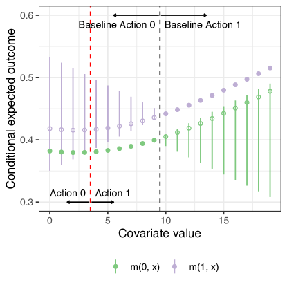
To further illustrate this case, consider the following numerical example where the action has a constant effect on the logit scale: where is a covariate-specific intercept for each . Suppose that the baseline action is given by . Under this setting, the solid points in Figure 2 indicate the identifiable values of , colored by the action (action 1 is green; action 0 is purple), while the hollow points represent the unidentifiable values. Each line shows a partial identification region, the range between the lower and upper bounds in Equation (6) above with the true Lipschitz constants and . Note that the intervals are not necessarily symmetric around the true values of the conditional expected outcome, as the lower and upper bounds represent the entire range of possibilities.
Since the treatment effect is always positive, the oracle policy that optimizes the true value, , would assign action 1 everywhere. To construct the robust policy via Equation (7), we assign action 1 wherever we can guarantee that action 1 has a higher expected outcome than action 0, or vice versa for action 0, no matter the true underlying model. These are the values where the solid points are entirely above (between red and black dashed lines) or below (right of the black dashed line) the partial identification lines. Wherever there is no such guarantee—where the lines contain the solid points (left of the red dashed line)—the maximin policy falls back to the baseline. The result is the robust policy that assigns action 1 for and action 0 otherwise. This safe policy improves welfare by 2.5% relative to the baseline, compared to the optimal rule which improves welfare by 4.2%.
3.3.2 Two binary covariates
Next, we consider a case with two binary covariates — again drawn uniformly for simplicity — where the utility changes are constant, i.e., , the cost is zero, i.e., , and a baseline policy assigns action 1 when both covariate values are 1, . Then, we can represent any conditional expectation function as a linear model with an interaction term, . Denote the conditional expectation of the observed outcome as . With this setup, the coefficients must satisfy the following four linear constraints:
| (8) | ||||||
Without any further assumptions, we can only identify , , and . Therefore, we cannot learn any policy other than the baseline policy without restrictions on the unidentifiable coefficients. It turns out, however, that if we are willing to assume that the conditional expectation is additive, i.e., for both actions, we can make progress. Under this additional assumption, we can represent these models as 3 dimensional vectors,
Then, the restricted set consists of vectors that satisfy the four linear constraints in Equation (8).
Using linear algebra tools, we can write the restricted set in terms of the observable model values and the null space of the four linear constraints. Specifically, the coefficients under action 0 are uniquely identified: , , and . In contrast, the coefficients for action 1 are only restricted to sum to . By computing the null space of this single constraint, the restricted model set can be written as,
Optimizing over the two unknown parameters, , we find the following worst-case value:
where is equal to if and is equal to otherwise. When finding the safe policy, this constrains the policy so that for all or . Thus, the maximin robust optimization problem (5) is given by,
Note that the only free parameter in the robust optimization problem is the policy action at ; the three other policy values are constrained to be zero. Therefore, with a fully flexible policy class, the robust policy is constrained to agree with the baseline policy for all but can still disagree for by extrapolating with the model. When the candidate policy gives an action of zero, , the worst-case value will use the point-identified control model, extrapolating to the unobserved case as . This allows us to learn a safe policy that can disagree with and will assign action 0 rather than action 1 if .
3.4 Regret relative to the baseline and oracle policies
We now derive the theoretical properties of the proposed population safe policy . To simplify the statements of the results, we will assume that the utility gain across different actions is constant and, without loss of generality, is positive, for all actions . First, the proposed policy is shown to be “safe” in the sense that it never performs worse than the baseline policy . This conservative principle is the key benefit of the robust optimization approach. The following proposition shows that as long as the baseline policy is in our policy class , and the underlying model lies in the restricted model class , the value of the population safe policy is never less than that of the baseline policy.
Proposition 1 (Population safety).
Let be a solution to Equation (5). If , and , then .
However, this guarantee of safety comes at a cost. In particular, the population safe policy may perform much worse than the infeasible, oracle optimal population policy, . Although we never know the oracle policy, we can characterize the optimality gap, , which is the regret or the difference in values between the proposed robust policy and the oracle.
To do this, we consider the “size” of the restricted model class . Specifically, we define the width of some function class in the direction of function as:
| (9) |
This represents the difference between the maximum and minimum cross-moment of a function and all possible functions . We then define the overall size of the model class, , as the maximal width over all possible policies:
where is the space of all possible policies. The size of the restricted model class denotes the amount of uncertainty due to partial identification. If we can point identify the conditional expectation function, then the size will be zero; larger partial identification sets will have a larger size.
The following theorem shows that the optimality gap, scaled by the utility gain , is bounded by the size of the model class. In other words, the cost of robustness is directly controlled by the amount of uncertainty in the restricted model class .
Theorem 1 (Population optimality gap).
Let be a solution to Equation (5). If , the regret of relative to the optimal policy is
In the limiting case where we can fully identify the conditional expectation , contains only one element. Then, the size will be zero and so the regret will be zero. This means that the solution to the robust optimization problem in Equation (5) will have the same value as the oracle, reducing to the standard case where we can point identify the conditional expectation. Conversely, if we can only point identify the conditional expectation function for few action-covariate pairs, then the size of the restricted model class will be large, there will be a greater potential for sub-optimality due to lack of identification, and the regret of the safe policy relative to the infeasible optimal policy could be large. Finally, note that the size of the restricted model class gives the worst-case bound, but the potentially tighter bound depends on the policy class as well.
4 The Empirical Safe Policy
In practice, we do not have access to an infinite amount of data, and so we cannot compute the population safe policy. Here, we show how to learn an empirical safe policy from observed data of finite sample size.
4.1 From the population problem to the empirical problem
Suppose we have independently and identically distributed data points . From this sample we wish to find a robust policy empirically. To do so, we begin with a sample analog to the value function in Equation (3) above,
| (10) |
With this, we could find the worst-case sample value across all models in the restricted model class from Equation (4). However, we do not have access to the true conditional expectation and so cannot compute the true restricted model class. One possible way to address this is to obtain an estimator of the conditional expectation function, , and use the estimate in place of the true values. However, this does not take into account the estimation uncertainty, and could lead to a policy that improperly deviates from the baseline due to noise. This approach will have no guarantee that the new policy is at least as good as the baseline without access to many samples: it would rely on convergence of the model for , which may be slow.
Instead, we construct a larger, empirical model class , based on the observed data, that contains the true restricted model class with probability at least ,
| (11) |
Then we construct our empirical policies by finding the worst-case in-sample value then maximizing this objective across policies
| (12) |
We discuss concrete approaches to constructing the empirical model class and solving this optimization problem in Section 5.1. In general, the empirical model class will be larger than the true model class and so a policy derived from it will be more conservative.
4.2 Finite sample statistical properties
What are the statistical properties of our empirical safe policy in finite samples? We will first establish that the proposed policy has an approximate safety guarantee: with probability approximately we can guarantee that it is at least as good as the baseline, up to sampling error and the complexity of the policy class. We then characterize the empirical optimality gap and show that it can be bounded using the complexity of the policy class as well as the size of the empirical restricted model class. For simplicity, we will consider the special case of a binary action set . We use the population Rademacher complexity to measure the complexity of the policy class:
where ’s are i.i.d. Rademacher random variables, i.e., , and the expectation is taken over both the Rademacher variables and the covariates . The Rademacher complexity is the average maximum correlation between the policy values and random noise, and so measures the ability of the policy class to overfit.
First, we establish a statistical safety guarantee analogous to Proposition 1.
Theorem 2 (Statistical safety).
Let be a solution to Equation (12). Given the baseline policy and the true conditional expectation , for any , the regret of relative to the baseline is,
with probability at least , where .
Theorem 2 shows that the regret for the empirical safe policy versus the baseline policy is controlled by the Rademacher complexity of the policy class , and an error term due to sampling variability that decreases at a rate of . The complexity of the policy class determines the quality of the safety guarantee for any level . If the policy class is simple, then the bound will quickly go towards zero for any level ; if it is complex, then we will require larger samples to ensure that the safety guarantee is meaningful, regardless of the level .
Importantly, by taking a conservative approach using the larger model class , the estimation error for the conditional expectation does not directly enter into the bound. However, if we cannot estimate well, the empirical restricted model class will be large, which will affect how well the empirical safe policy compares to the oracle policy. To quantify this, we will again rely on a notion of the size of the empirical restricted model class . In this setting, however, we will use an empirical width,
| (13) |
Similarly to above, we define the empirical size of , , as the maximal empirical width over potential models,
Theorem 3 (Empirical optimality gap).
Let be a solution to Equation (12) and assume that the utility gains are equal to each other, . If the true conditional expectation , then for any , the regret of relative to the optimal policy is
with probability at least , where .
Comparing to Theorem 1, we see that the size — now the empirical version — plays an important role in bounding the gap between the empirical safe policy and the optimal policy. In addition, the Rademacher complexity again appears: policy classes that are more liable to overfit can have a larger optimality gap. For many standard policy classes, we can expect the Rademacher complexity to decrease to zero as the sample size increases, while the empirical size of the restricted model class may not. Furthermore, there is a tradeoff between finding a safe policy with a higher probability — setting the level to be high — and finding a policy that is closer to optimal. By setting to be high, the width of will increase, and the potential optimality gap will be large. This tradeoff is similar to the tradeoff between having a low type I error rate ( low) and high power ( low) in hypothesis testing. Similarly, if we cannot estimate the conditional expectation function well, then the size can be large even with low probability guarantees .
5 Model and Policy Classes
The two important components when constructing safe policies are the assumptions we place on the outcome model — the model class — and the class of candidate policies that we consider . We will now consider several representative cases of model classes, show how to construct the restricted model classes, and apply the theoretical results above. Then, we will further discuss the role of the policy class, considering the special cases of the results for policy classes with finite VC dimension.
5.1 Point-wise bounded restricted model classes
We now give several examples of model classes and the restricted model classes induced by the data . For all of the model classes we consider, the restricted model class will be a set of functions that are upper and lower bounded point-wise by two bounding functions,
| (14) |
We will also create an empirical restricted model class that satisfies the probability guarantee in Equation (11). This similarly results in the form of a point-wise lower and upper bound on the conditional expectation function, with lower and upper bounds and , respectively. These point-wise bounds yield a closed form bound on the size of the restricted model class and the empirical size of the empirical restricted model class as the expected maximum difference between the bounds:
| (15) |
In Appendix A.1 we use these bounds to specialize Theorems 1 and 3 to this case.
The point-wise bound also allows us to solve for the worst-case population and empirical values and by finding the minimal value for each action-covariate pair (see Pu and Zhang, 2021). Finding the empirical safe policy by solving Equation (12) is equivalent to solving an empirical welfare maximization problem using a quasi-outcome that is equal to the observed outcome when the action agrees with the baseline policy, and is equal to either the upper or lower bound when it disagrees,
With this, Equation (12) specializes to
| (16) |
In effect, for an action where the baseline action is equal to , the minimal value uses the outcomes directly. In the counterfactual case where the baseline action is different from , the value will use either the upper or lower bound of the outcome model, depending on the sign of the utility gain. Using bounds in place of outcomes in this way is similar to the approach of Pu and Zhang (2021) in instrumental variable settings. Since the optimization problem (16) is not convex, it is not straightforward to solve exactly. As many have noted (e.g. Zhao et al., 2012; Zhang et al., 2012; Kitagawa and Tetenov, 2018), this optimization problem can be written as a weighted classification problem and approximately solved via a convex relaxation with surrogate losses. An alternative approach is to solve the problem in Equation (16) directly. In our empirical studies, we consider thresholded linear policy classes that mirror the NVCA and DMF rules we discuss in Section 2; these turn Equation (16) into a mixed integer program that we can solve efficiently with commercial solvers. Alternatively, we can use the approach for finite-depth decisions tree policies implemented in Sverdrup et al. (2020), and for continuous, non-deterministic policies (or approximations to deterministic ones) we could use stochastic gradient descent methods designed to escape from local minima.
We now give several examples of model classes that lead to point-wise bounded restricted model classes, deferring derivations and additional examples to Appendix A.2.
Example 1 (No restrictions).
Suppose that the conditional expectation has no restrictions, other than that it lies between zero and one, i.e., . Then the restricted model class provides no additional information when the policy disagrees with the baseline policy and the upper and lower bounds in Equation (14) are and , respectively. In the absence of any additional information, the worst case conditional expectation is 0 or 1 (depending on the sign of the utility gain) whenever it is not point identified. The size of this model class is then , the maximum possible value. Note, however, that it is still possible to learn a new policy if the utility gain for an action is never worth the cost, i.e., .
To construct the larger, empirical model class , we begin with a simultaneous confidence interval for the conditional expectation function , with lower and upper bounds such that
| (17) |
See Srinivas et al. (2010); Chowdhury and Gopalan (2017); Fiedler et al. (2021) for examples on constructing such simultaneous bounds via kernel methods in statistical control settings. With this confidence band, we can use the upper and lower bounds of the confidence band in place of the true conditional expectation , i.e. and .
Example 2 (Lipschitz Functions).
Suppose that the covariate space has a norm , and that is a -Lipschitz function,
Taking the greatest lower bound and least upper bound implied by this model class leads to lower and upper bounds, , and , where recall that is the set of covariates where the baseline policy gives action . The further we extrapolate from the area where the baseline action , the larger the value of will be and so there will be more ignorance about the values of the function. So the size of will depend on the expected distance to the boundary between baseline actions and the value of the Lipschitz constant. If most individuals are close the boundary, or the Lipschitz constant is small, will be small and the safe policy will be close to optimal. Conversely, a large number of individuals far away from the boundary or a large Lipschitz constant will increase the potential for suboptimality. To construct the empirical version, we again use a simultaneous confidence band satisfying Equation (17). Then the lower and upper bounds use the lower and upper confidence limits in place of the function values, and .
Example 3 (Generalized linear models).
Consider a model class that is a generalized linear model in a set of basis functions , with monotonic link function , . The restricted model class is the set of coefficients that satisfy for all and such that . Let be the minimum norm solution and let be an orthonormal basis for the null space . Then we can re-write the restricted model class as
The free parameters in this model class are represented as the vector . Finding the worst-case value will involve a non-linear optimization over , which may result in optimization failure. Rather than taking this approach, we will consider a larger class that contains the restricted model class . Note that using this larger model class will be conservative. Since is between 0 or 1, we can use this bound when is in the null space to get upper and lower bounds
The worst-case value uses to extrapolate wherever we can point identify . It resorts to one of the bounds for units assigned to action when and is not orthogonal to the null space. The size of the model class is the percentage of units that are in the null space, . The fewer units in the null space, the smaller the size and the closer the safe policy is to optimal.
To construct the empirical model class we again begin with a simultaneous confidence band, this time for the minimum norm prediction via the Working-Hotelling-Scheffé procedure (Wynn and Bloomfield, 1971; Ruczinski, 2002),
where is the least squares estimate of the minimum norm solution, is the estimate of the variance from the MSE, is the design matrix, is the rank of , is the quantile of an distribution with and degrees of freedom, and denotes the pseudo-inverse of a matrix . This gives lower and upper bounds,
5.2 Policy classes with finite VC dimension
The choice of model class corresponds to the substantive assumptions we place on the outcomes in order to extrapolate and find new policies. The choice of policy class is equally important: it determines the type of policies we consider. An extremely flexible policy class with no restrictions will result in the highest possible welfare, but such a policy is undesirable for two reasons. First, they are all but inscrutable by both those designing the algorithms and those subject to the algorithm’s actions (see Murdoch et al., 2019, for discussion on interpretability issues). Second, policies that are too flexible will have a high complexity, and so the bounds on the regret of the empirical safe policy—versus either the baseline policy or the infeasible optimal policy—will be too large to give meaningful gaurantess.
One way to characterize the complexity of the policy class is via its VC-dimension: the largest integer for which there exists some points that are shattered by , i.e. where the policy values can take on all possible combinations (for more on VC dimension and uniform laws, see Wainwright, 2019, §4). Examples of policy classes with finite VC dimension include linear policies, with a VC dimension of , and depth decision trees with VC dimension on the order of (Athey and Wager, 2021).
The VC dimension gives an upper bound on the Rademacher complexity: for a function class with finite VC dimension , the Rademacher complexity is bounded by, , for some universal constant (Wainwright, 2019, §5.3). In Appendix A.3, we use this bound to specialize the results in Section 4.2, finding that the higher the VC dimension, the more liable a policy is to overfit to the noisy data, and the more samples we will need to ensure that the regret bound is low. For a policy class with finite VC dimension, which will be typical in applied policy settings, the rate of convergence will still be . However, for a policy class with VC dimension growing with the sample size, , the rate of growth must be less than in order for the regret to converge to a value less than or equal to zero. See Athey and Wager (2021) for further discussion.
6 Extensions
Motivated by our application introduced in Section 2, we consider two important extensions of the methodology proposed above. First, we consider the scenario under which the data come from a randomized experiment, where a deterministic policy of interest is compared to a status quo without such a policy. Second, we consider a human-in-the-loop setting, in which an algorithmic policy recommendation is deterministic, but the final decision is made by a human decision-maker in an unknown way. In this case, we must adapt the procedure to account for the fact that the policy may affect the final decisions, but does not determine them, implying that actions only incur costs through the final decisions. For notational simplicity, we will again assume, throughout this section, that the utility gain is constant across all actions and is denoted by .
6.1 Experiments evaluating a deterministic policy
In many cases, a single deterministic policy is compared to the status quo of no such policy via a randomized trial for program evaluation. In our empirical study, the existing policy was compared to a “null” policy where no algorithmic recommendations were provided. The goal of such a trial is typically to evaluate whether one should adopt the algorithmic policy. We now show that one can use the proposed methodology to safely learn a new, and possibly better, policy even in this setting. In particular, we can weaken the restrictions of the underlying model class by placing assumptions on treatment effects rather than the expected potential outcomes. We focus here on comparing a baseline policy to a null policy that assigns no action, which we denote as , and has potential outcome .
In this setup, let be a treatment assignment indicator where if no policy is enacted (i.e., null policy), and if the policy follows the baseline policy . Let be the probability of assigning the treatment condition for an individual with covariates . Since it is an experiment, this probability is known. Rather than minimize the regret relative to the baseline policy as in Equation (5), we will minimize regret relative to the null policy . Defining the conditional average treatment effect (CATE) of action relative to no action , , we can now write the regret of a new policy relative to the null policy as,
Now, following Kitagawa and Tetenov (2018), we can identify the the CATE function for the baseline policy using the transformed outcome , which equals the CATE in expectation, i.e., . With this, we follow the development in Section 3.2, with the transformed outcome replacing the outcome and a restricted model class for the treatment effects replacing the model class for the outcomes . Specifically, we decompose the regret into an identifiable component and an unidentifiable component, and consider the worst-case regret across all treatment effects in , giving the population robust optimization problem,
| (18) |
We can similarly construct the empirical analog by creating a larger empirical model class as in Section 4.
From the perspective of finding a new, empirical safe policy , the key benefit of experimentally comparing two deterministic policies in this way is that the primary unidentified object is the CATE, , rather than the conditional expected potential outcome, . Treatment effect heterogeneity is often considered to be significantly simpler than heterogeneity in outcomes (see, e.g., Künzel et al., 2019; Hahn et al., 2020; Nie and Wager, 2021). Therefore, we may consider a smaller model class for the treatment effects than the class for the conditional expected outcomes , leading to better guarantees on the optimality gap between the robust and optimal policies in Theorems 1 and 3.
6.2 Algorithm-assisted human decision-making
In many cases, an algorithmic policy is not the final arbiter of decisions. Instead, there is often a “human-in-the-loop” framework, where an algorithmic policy provides recommendations to a human that makes an ultimate decision. Our pre-trial risk assessment application is an example of such algorithm-assisted human decision-making (Imai et al., 2020).
To formalize this setting, let be the potential (binary) decision for individual under action (or an algorithmic recommendation in our application) , and be the potential (binary) outcome for individual under decision and action . We denote the expected potential decision conditional on covariates as . Further, we denote the potential outcome under action as and again represent the conditional expectation by . Then, the observed decision is given by whereas the observed outcome is . Finally, we write the utility for outcome under decision as .
With this setup, the value for a policy is:
We make the simplifying assumption that the utility gain is constant across decisions, for , index the utility for and as , and denote the added cost of taking decision 1 as . Now we can write the value by marginalizing over the potential decisions, yielding,
| (19) |
Comparing Equation (19) to the value in Equation (1) when actions are taken directly, we see that the key difference is the inclusion of the potential decision in determining the cost of an action. Rather than directly assigning a cost to an action , there is an indirect cost associated with the eventual decision that action induces in the decision maker. Therefore, lack of identification of the expected potential decision under an action given the covariates, , also must enter the robust procedure.
We can treat lack of identification of the potential decisions in a manner parallel to the outcomes. Denoting the conditional expected observed decision as , we can posit a model class for the decisions and created the restricted model class .333These restrictions being on the decisions gives more opportunities for structural restrictions on the model. For example, we could make a monotonicity assumption that for . We can now create a population safe policy by maximizing the worst case value across the model classes for both the outcomes and the decisions ,
| (20) | ||||
By allowing for actions to affect decisions through the decision maker rather than directly, the costs of actions are not fully identified. Therefore, we now find the worst-case expected outcome and decision when determining the worst case value in Equation (20). In essence, we solve the inner optimization twice: once over outcomes for the restricted outcome model class and once over decisions for the restricted decision model class .
From here, we can follow the development in the previous sections. We create empirical restricted model classes for the outcome and decision functions, and using a Bonferonni correction so that . Then, we solve the empirical analog to Equation (20). Finally, we can incorporate experimental evidence as in Section 6.1. In this case, the conditional expected potential decision and outcome — and their model classes — are replaced with the conditional average treatment effect on the decision and on the outcome .
7 Empirical Analysis of the Pre-trial Risk Assessment
We now apply the proposed methodology to the PSA-DMF system and the randomized controlled trial described in Section 2. We will focus on learning robust rules for two aspects of the PSA-DMF system: the way in which the binary new violent criminal activity (NVCA) flag is constructed and the overall DMF matrix recommending a signature bond or cash bail. For both settings, we use the incidence of an NVCA as the outcome. In Appendix C, we also inspect the behavior of this methodology via a Monte Carlo simulation study.
7.1 Learning a new NVCA flag threshold
We begin by learning a new threshold for the NVCA flag. Let be the total number of NVCA points for an arrestee, computed using the point system in Table 1. Recall that the baseline NVCA algorithm is to trigger the flag if the number of points is greater than or equal to 4, i.e. . Our goal in this subsection is to find the optimal worst-case policy across the set of threshold policies,
| (21) |
where our binary outcome of interest is no NVCA occurring. Here, we will keep the baseline weighting on arrestee risk factors and only change the threshold ; in Section 7.2 below we will turn to changing the underlying weighting scheme.
Having chosen the policy class , we need to restrict the conditional average treatment effect on no NVCA occurring, . Here, we impose a Lipschitz constraint on the CATE, following Example 2. We also restrict the treatment effects to be bounded between and 1, since the outcome is binary. Note that this is not the tightest possible bound, since the restriction is that . To incorporate the uncertainty in estimating in finite samples we could use analogous techniques to those in Section 4; we leave this to future work.
For this model class, we need to specify the Lipschitz constants for the CATE when the flag is and is not triggered ( for and for , respectively). We adapt a heuristic suggestion from Imbens and Wager (2019) for model classes with a bounded second derivative to the Lipschitz case. We estimate the CATE function by taking the difference in NVCA rates with and without provision of the PSA at each level of . Then, we choose the Lipschitz constants to be three times the largest consecutive difference between CATE estimates, yielding and , though other choices are possible. In Appendix C, we inspect the impact of this multiplicative factor on the performance of the empirical safe policy through a simulation study. To construct the empirical restricted model class, we set the level to , allowing some tolerance for statistical uncertainty, and construct a simultaneous 80% confidence interval for the CATE via the Working-Hotelling-Scheffé procedure, as in Example 3, and use the upper and lower confidence limits.
The next important consideration in constructing a new policy is the form of the utility function. Recall that in our parameterization we must define the difference in utilities when there is and is not a new violent criminal activity, , for both actions . Similarly, we need to define the baseline “cost” of action , . While the marginal monetary cost of triggering the NVCA flag versus not can be considered approximately zero given the initial fixed cost of collecting the data for the PSA, there are other costs to consider. For instance, to the extent that triggering the NVCA flag increases the likelihood of pre-trial detention, it will lead to an increase in fiscal costs — e.g., housing, security, and transportation — directly incident on the jurisdiction. Furthermore, there are potential socioeconomic costs to the defendant and their community. To represent these costs, we will place zero cost on not triggering the NVCA flag, , and a cost of 1 on triggering the flag, . We then assign an equal utility gain from avoiding an NVCA, (equivalently, the cost of an NVCA is ). This yields a utility function of the form . We will consider how increasing the cost of an NVCA relative to the cost of triggering the flag changes the policies we learn.
Figure 3 shows the results. It represents the empirical restricted model class by showing point estimates and simultaneous 80% confidence intervals for the observable component of the CATE function and the partial identification set for the unobservable component. Notice that there is substantially more information when extrapolating the CATE for the case that the NVCA flag is not triggered. As we can see in Figure 3, this is because the point estimates do not vary much with the total number of NVCA points, and so we use a small Lipschitz constant. On the other hand, there is essentially no information when extrapolating in the other direction. Because there is a large jump in the point estimates between and , we use a large Lipschitz constant. This means that the empirical restricted model class puts essentially no restrictions on for : the treatment effects can be anywhere between and .
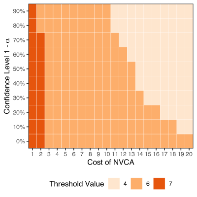
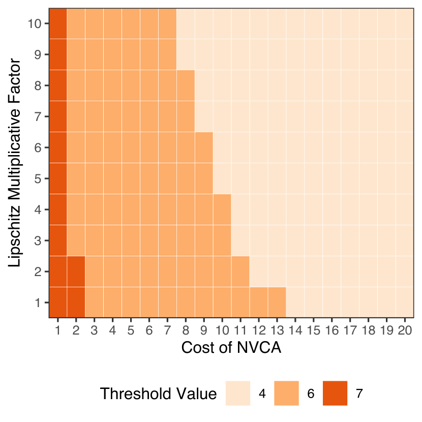
While the treatment effects are ambiguous, we can still learn a new threshold because we assign a cost to triggering the NVCA flag. To compute the empirical robust policy we can solve Equation (16) via an exhaustive search, since the policy class only has eight elements. Solving this for different costs of an NVCA, we find that when the cost is between 1 and 11 times the cost of triggering the flag — that is, — the new robust policy is to set the threshold to , only triggering the flag for arrestees with the observed maximum of 6 total NVCA points. This is a much more lenient policy, reducing the number of arrestees that are flagged as at risk of an NVCA by 95%. Conversely, when the cost of an NVCA is 11 times the cost of triggering the flag or more, the ambiguity about treatment effects leads the empirical safe policy to revert to the status quo, keeping the threshold at . In Figure D.2 of the Appendix, we show how the maximin threshold changes as we vary the confidence level and the multiplicative factor on the estimated Lipschitz constant; overall the relationship between the threshold and the cost of an NVCA is robust to the particular choices.
7.2 Learning a new NVCA flag point system
We now turn to constructing a new, robust NVCA flag rule by changing the weights applied to the risk factors in Table 1. We use the same set of covariates as the original NVCA rule, represented as 7 binary covariates : binary indicators for current violent offense, current violent offense and 20 years old or younger, pending charge at time of arrest, prior conviction (felony or misdemeanor), 1 prior violent conviction, 2 prior violent convictions, and 3 or more prior violent convictions. The status quo system uses a vector of weights on the risk factors and triggers the NVCA flag if the sum of the weights is greater than or equal to four, i.e., . To simplify comparisons to the status quo, we will constrain the threshold to remain at 4, though we could additionally include the threshold as a decision variable.
Given this, a key consideration is the form of the policy class that we will use. We ensure that the new rule has the same structure as the status quo rule, making it easier to adapt the existing system and use institutional knowledge in the jurisdiction. Specifically, we use the following policy class that thresholds an integer-weighted average of the 7 binary covariates,
| (22) |
This policy class therefore includes the original NVCA flag rule as a special case (see Table 1). In addition, to understand any differences between policies in this class, we can simply compare the vector of weights .
7.2.1 Empirical size of potential model classes
We begin by defining several possible models for the outcomes. We consider two models of the conditional expected potential incidence of an NVCA: an additive outcome model class , and an outcome model with separate additive terms and common two-way interactions ,
We additionally restrict the outcome models to be bounded between zero and one. For these two model classes, we only use those cases where the NVCA flag was shown to the judge.
Because cases were randomly assigned to the control group for which the judge has no access to the PSA-DMF system, we can alternatively follow the development in Section 6.1 and use the structure of the experiment to place restrictions on the effect of assigning an NVCA flag of 1, . An advantage is that we can use both the cases that did and did not have access to the PSA. We consider two different treatment effect models: an additive effect model and a second order effect model ,
Here, we again restrict the treatment effects to be bounded between and 1.
These four model classes each lead to different restrictions, and ultimately affect what policies we can learn from this experiment. This is partly because even with infinite data the models may not be identifiable. But, it is also because with finite data there is a different amount of uncertainty on each model class. Figure 4 depicts this information by showing how the empirical size of the model class (vertical axis), defined in Equation (13), changes with the the desired confidence level (horizontal axis). Recall that the size when the confidence level is zero serves as a proxy for the population size of the model class defined in Equation (9).
For the additive outcome and effect models, the size is zero when the confidence level is zero, implying that these models are identifiable. This is due to the structure of the NVCA flag rule: for given values of the covariates, it is possible to observe cases with the flag set to zero or one. When taking into account the statistical uncertainty, the widths increase. This is primarily due to greater uncertainty for cases with a flag of 1, which account for only 16% of the cases. The size for flag 1 (orange) determines the overall size (purple) and so the lines overlap.
The two model classes also differ in how they vary with the confidence level; there is more uncertainty in the treatment effect and so the size of the additive effect model is larger at every value of the confidence level than the additive outcome model. However, the additive treatment effect assumption is significantly weaker than the additive outcome assumption. Relative to the two additive models, the second order models have significantly more uncertainty reflected in larger empirical sizes. This is primarily due to the lack of identification; even without accounting for statistical uncertainty, the widths are already over 75% of their maximum values. Indeed, there are many combinations of the binary covariates where we cannot observe cases that have an NVCA flag of both zero and one. For example, there are only 28 cases (1.5% of the total) where we can identify the model for both values. Moreover, all of these cases have the same characteristics: the arrestee has committed a violent offense, is over 21 years old, has a pending charge, and a prior felony or misdemeanor conviction.
The empirical size of the model class gives an indication of the potential optimality gap between the empirical safe policy we learn and the true optimal policy. Unfortunately, this statistic does not describe how flexible the class is and whether we should expect it to contain the true relationship between the potential outcomes and the covariates, since it only describes how much of the model is left unidentified. These considerations are crucial to guarantee robustness. The additive outcome model has the smallest size overall, but it also places the strongest restrictions. It is contained by the second order interaction outcome model , but this model has a much larger size.
Choosing between these two models represents a tradeoff: the larger model is more liable to contain the truth and so we can guarantee a greater degree of robustness, but choosing the smaller model can yield a better policy if it does indeed contain the truth. In contrast, the additive treatment effect class both is weaker than the second order outcome model and has a smaller empirical size. Therefore, we can make weaker assumptions without limiting our ability to find a good policy as much. This is the key benefit of incorporating the control information in this study.
Note that the second order treatment effect model, which makes the weakest assumptions, is too large to provide any guarantees on the regret relative to the optimal policy. Therefore, for the reminder of this section, we focus on the additive treatment effect model, which allows us to include the control group information and make weaker assumptions than the additive outcome model.
7.2.2 Constructing a robust NVCA flag rule
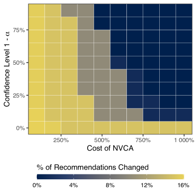
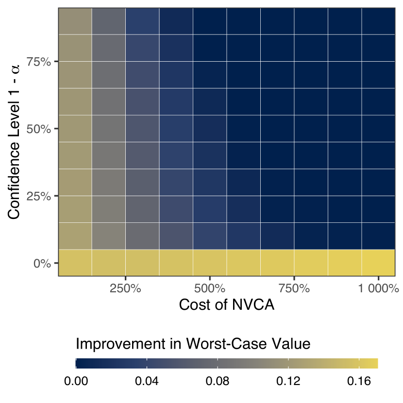
Figure 5 shows how the robust policy, which solves the optimization problem given in Equation (16) with the additive treatment effect class , compares to the original rule as we vary the cost of an NVCA (horizontal axis) and the confidence level (vertical axis). With the integer-weighted policy class , the optimization problem is an integer program; we solve this with the Gurobi solver (Gurobi Optimization, LLC, 2021). The left panel shows the percent of recommendations changed from the original ones, while the right panel displays the improvement in the worst-case value over the original NVCA flag rule. Across every confidence level, the robust policy differs less and less from the original rule as the cost of an NVCA relative to the cost of triggering the flag increases. For a given cost of an NVCA, policies at lower confidence levels are more aggressive in deviating from the original rule, prioritizing a potentially lower regret relative to the optimal policy at the expense of guaranteeing that the new policy is no worse than the original rule.
Figure 6 inspects the integer-weights on the risk factors for the robust policy at the level, as the cost of an NVCA increases. In the limiting setting where an NVCA is given the same cost as triggering the NVCA flag, the robust policy differs substantially from the original rule, placing no weight on prior violent convictions. Once the cost is at least five times the cost of triggering the flag, the robust policy reduces to the original rule. For intermediate values, the robust policy places less — but not zero — weight on the number of prior violent convictions than the original rule.
In light of the empirical sizes displayed in Figure 4, this behavior is primarily due to increased uncertainty in the effect of triggering the NVCA flag relative to not. When the cost of an NVCA is low, the robust policy will not trigger the NVCA flag for cases that triggered the original flag; even with the increased uncertainty, it is preferable in these cases to not trigger the flag. Conversely, when the cost of an NVCA is high the increased uncertainty in the effect of triggering the flag makes the robust policy default to the original rule. In this case, the high costs of an NVCA make any change in the policy too risky to act upon.
7.2.3 Incorporating judge’s decisions
So far, we have only considered the outcomes of triggering the NVCA flag and have assigned costs directly to the flag. However, the PSA serves as a recommendation to the presiding judge who is the ultimate decision maker. Following the discussion in Section 6.2 we can incorporate this into the construction of the robust policy. Rather than place a cost on triggering the NVCA flag, we use the judge’s binary decision of whether to assign a signature bond or cash bail, and place a cost of to assigning cash bail. Unlike the cost on the NVCA flag above, this allows us to address the costs of detention directly. As discussed above, the cost on the judge’s decision to assign cash bail includes the fiscal and socioeconomic costs, indexed to be .
Following the same analysis as above, we can find robust policies that take the decisions into account for increasing costs of an NVCA relative to assigning cash bail, at various confidence levels. However, for the additive and second order effect models we find policies that differ from the original rule only when we do not take the statistical uncertainty into account — with confidence level — and have no finite sample guarantee that the new policy is not worse than the existing rule. In this case, the policy is extremely aggressive, responding to noise in the treatment effects. Otherwise, we cannot find a new policy that safely improves on the original rule. This is primarily because the overall effects of the PSA on both the judge’s decisions and defendants behavior are small (Imai et al., 2020); therefore there is too much uncertainty to ensure that a new policy would reliably improve upon the existing rule.
7.3 DMF Matrix
Another key component of the the PSA-DMF framework is the overall recommendation given by the DMF matrix (see Figure 1). This aggregates the FTA and NCA scores into a single recommendation on assigning a signature bond versus cash bail. We now consider constructing a new DMF matrix based on the FTA and NCA scores, which we combine into a vector . We restrict our analysis to the 1,544 cases that used the DMF matrix rather than those that cash bail was automatically assigned.
Here, we again focus on the class of additive treatment effect models , where we only condition on the FTA and NCA scores since they are the two components of the DMF decision matrix. Because and are discrete with six values, we can further parameterize the additive terms as six dimensional vectors. Importantly, this rules out interactions between the FTA and NCA scores in the effect. If this assumption is not credible, we could use a Lipschitz restriction as in Example 2. This alternative assumption may be significantly weaker, though it would require choosing the Lipschitz constant.
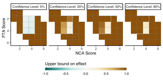
To understand how this additive treatment effect model facilitates robust policy learning, we inspect the upper bounds on the treatment effects as the confidence level changes. Figure 7 shows these bounds for the different values of the FTA and NCA scores. As in Section 7.2 above, the bounds with zero confidence level correspond to bounds induced by the model class in the population. Because we can never observe a case where the DMF recommends a signature bond with either an FTA score or NCA score above 4, we cannot identify the additive model components for either variable above 4. Because of this, the upper bound on the effect of recommending a signature bond for these cases is 1, the maximum value.
Similarly, we can never observe a case where the DMF recommends cash bail with either an FTA score below 2 or an NCA score below 3. This precludes assigning cash bail to these cases. In the middle is an intermediate area with FTA scores between 2 and 4 and NCA scores between 3 and 4 where we can fully identify the effect of assigning cash bail under the additive model. Note that unlike the NVCA threshold above, this means that new policies can only differ from the status quo in the less lenient direction, recommending cash bail for arrestees that would have a signature bond recommendation under the status quo. However, for values with an FTA score of 2 or an NCA score of 3, there is a significant amount of uncertainty due to small sample sizes. Indeed, there are only 3 cases where cash bail is recommended that have an NCA score of 3 and 2 cases that have an FTA score of 2.
To search for new policies, we consider a policy class that is monotonically increasing in both covariates. This monotonic policy class contains the DMF matrix rule as a special case and incorporates the notion that no case should move from a cash bail to a signature bond recommendation if the risk of an FTA or NCA increases. Formally, this monotonic policy class is given by,
As in Section 7.2, we consider parameterizing the utility in terms of a fixed cost of 1 for recommending cash bail — reflecting the fiscal and socioeconomic costs of detention — and varying the cost of an NVCA.
Figure 8 shows the robust policies learned for the varying cost of an NVCA and different confidence levels. In the limiting case where the cost of an NVCA is equal to recommending cash bail, the safe policy is to assign a signature bond for all but the most extreme cases. This is because even if assigning a signature bond is guaranteed to lead to an NVCA, the utility is equal to assigning cash bail and not leading to an NVCA.444This is a consequence of the looser bound that the treatment effects are bounded between and . If instead we used the sharper bound that — and properly accounted for boundary effects — the safe policy would never assign cash bail. In the other limiting case, we eschew finite sample statistical guarantees and set the confidence level to 0. That is, we ignore any statistical uncertainty in estimating the conditional expectation function, and instead use the point estimate directly. When doing this, increasing the cost of an NVCA relative to recommending cash bail leads to more of the intermediate area with FTA scores between 2 and 4 and NCA scores between 3 and 4 being assigned cash bail, until the cost is high enough that the entire identified area is assigned cash bail. However, this does not hold up to even the slightest of statistical guarantees due to the uncertainty in the treatment effects. Because the effects of assigning cash bail are both small and uncertain, the robust policy reduces to the existing DMF matrix.
8 Discussion
In recent years, algorithmic and data-driven policies and recommendations have become an integral part of our society. Being motivated in part by this transformative change, the academic literature on optimal policy learning has flourished. The increasing availability of granular data about individuals at scale means that the opportunities to put these new methodologies in practice will only grow more in the future.
One important challenge when learning and implementing a new policy in the real world is to ensure that it does not perform worse than the existing policy. This safety feature is critical, especially if relevant decisions are consequential. In this paper, we develop a robust optimization approach to deriving an optimal policy that has a statistical safety guarantee. This allows policy makers to limit the probability that a new policy achieves a worse outcome than the existing policy.
The development of a safe policy is essential particularly when it is impossible to conduct a randomized experiment for ethical and logistical reasons. Observational studies bring additional uncertainty due to the lack of identification. Moreover, for transparency and interpretability, most policies are based on known, deterministic rules, making it difficult to learn a new policy using standard methods such as inverse probability-of-treatment weighting. We develop a methodology that addresses these challenges and apply it to a risk assessment instrument in the criminal justice system. Our analysis suggests an opportunity for improving the existing scoring rules.
An important aspect of this methodology is that it depends on the design of the baseline policy. The structure of the baseline will determine what is identifiable and what is not. For example, in the PSA-DMF system we explore here, we were able to fully identify additive models because the NVCA scoring rule incorporates several risk factors and no single risk factor guarantees that the flag will fire. On the other hand, we could not fully identify an additive model for the DMF matrix because if either the NCA or FTA scores are large enough, the recommendation is always cash bail. This logic extends to higher dimensions. For example, we could not identify many terms in the interactive effect model because most combinations of two risk factors result in an NVCA flag. Therefore, this framework is likely to be most successful for policies based on several covariates that are aggregated to a single score before thresholding.
There are several avenues for future research. The first set of questions relates to the implementation choices under the proposed approach. While we consider several representative cases, there are many other structural assumptions that would lead to different forms of extrapolation. For instance, we could consider a global structure in the form of Reproducing Kernel Hilbert Spaces, or incorporate substantive restrictions such as monotonicity. In addition, while our study on pre-trial risk scores focused on discrete covariates, deterministic policies with continuous covariates opens the opportunity to directly identify treatment effects on the decision boundary, leading to a different form of restriction on the model class. We can also generalize this approach to consider cases where policies consist of both stochastic and deterministic components. This would nest the current deterministic case including the experimental setting discussed in Section 6.1.
Second, we can use similar statistical tools to create tests of safety for given policies. By creating a worst-case upper bound on the regret of a policy relative to the status quo, we can test for whether this upper bound is below zero, rejecting the null that the proposed new policy is not an improvement over the existing status quo.
Third, there are many ways in which optimal algorithmic recommendations may differ when considering long term societal outcomes rather than short term ones. For example, pre-trial detention brought on by a recommendation may in turn alter the long term behavior and welfare of an arrestee. Understanding how to design algorithms when they affect decisions that mediate future outcomes is key to ensuring that recommendations do not take a myopic view. One potential way to incorporate long term outcomes may be with the use of surrogate measures. More work needs to be done on the question of how to incorporate surrogate measures into our policy learning framework while providing a safety guarantee.
Finally, within the robust optimization framework, the notion of “safety” can be considerably expanded. In this paper, we consider policies to be safe if they do not lead to worse outcomes on average; however, this does not guarantee that outcomes are not worse for subgroups. A more equitable notion of safety would be to ensure safety across subgroups, though doing so may reduce the ability to improve overall welfare. Similarly, the robust optimization framework can be made to incorporate statistical fairness criteria — a different form of safety. Such constraints may be themselves uncertain or only partially identified, and so a robust approach would account for this as well (Imai and Jiang, 2020).
References
- Angwin et al. (2016) Angwin, J., J. Larson, S. Mattu, and L. Kirchner (2016). Machine bias: There’s software used across the country to predict future criminals. and it’s biased against blacks. https://www.propublica.org/article/machine-bias-risk-assessments-in-criminal-sentencing.
- Athey and Wager (2021) Athey, S. and S. Wager (2021). Policy Learning With Observational Data. Econometrica 89(1), 133–161.
- Balke and Pearl (1994) Balke, A. and J. Pearl (1994). Counterfactual Probabilities: Computational Methods, Bounds and Applications. In Proceedings of the Tenth Conference on Uncertainty in Artificial Intelligence, pp. 46–54.
- Bastani et al. (2021) Bastani, H., M. Bayati, and K. Khosravi (2021). Mostly exploration-free algorithms for contextual bandits. Management Science 67(3), 1329–1349.
- Bertsimas et al. (2011) Bertsimas, D., D. B. Brown, and C. Caramanis (2011). Theory and applications of robust optimization. SIAM Review 53(3), 464–501.
- Beygelzimer and Langford (2009) Beygelzimer, A. and J. Langford (2009). The offset tree for learning with partial labels. Proceedings of the ACM SIGKDD International Conference on Knowledge Discovery and Data Mining, 129–137.
- Center on Budget and Policy Priorities (2017) Center on Budget and Policy Priorities (2017). A Quick Guide to SNAP Eligibility and Benefits. Technical report.
- Chowdhury and Gopalan (2017) Chowdhury, S. R. and A. Gopalan (2017). On kernelized multi-armed bandits. 34th International Conference on Machine Learning, ICML 2017 2, 1397–1422.
- Coston et al. (2020) Coston, A., A. Mishler, E. H. Kennedy, and A. Chouldechova (2020). Counterfactual risk assessments, evaluation, and fairness. FAT* 2020 - Proceedings of the 2020 Conference on Fairness, Accountability, and Transparency, 582–593.
- Cui (2021) Cui, Y. (2021). Individualized decision making under partial identification: three perspectives, two optimality results, and one paradox. Harvard Data Science Review. Just accepted.
- Cui and Tchetgen Tchetgen (2021) Cui, Y. and E. Tchetgen Tchetgen (2021). A Semiparametric Instrumental Variable Approach to Optimal Treatment Regimes Under Endogeneity. Journal of the American Statistical Association 116(533), 162–173.
- Dieterich et al. (2016) Dieterich, W., C. Mendoza, and T. Brennan (2016). Compas risk scales: Demonstrating accuracy equity and predictive parity. http://go.volarisgroup.com/rs/430-MBX-989/images/ProPublica_Commentary_Final_070616.pdf. Northpointe Inc. Research Department.
- Dudik and Langford (2011) Dudik, M. and J. Langford (2011). Doubly Robust Policy Evaluation and Learning. In Proceedings of the 28th International Conference on Machine Learning.
- Fiedler et al. (2021) Fiedler, C., C. W. Scherer, and S. Trimpe (2021). Practical and Rigorous Uncertainty Bounds for Gaussian Process Regression. In Association for the Advancement of Artificial Intelligence.
- Greiner et al. (2020) Greiner, D. J., R. Halen, M. Stubenberg, and J. Chistopher L. Griffen (2020). Randomized control trial evaluation of the implementation of the psa-dmf system in dane county. Technical report, Access to Justice Lab, Harvard Law School.
- Gupta et al. (2020) Gupta, V., B. R. Han, S. H. Kim, and H. Paek (2020). Maximizing intervention effectiveness. Management Science 66(12), 5576–5598.
- Gurobi Optimization, LLC (2021) Gurobi Optimization, LLC (2021). Gurobi Optimizer Reference Manual.
- Hahn et al. (2020) Hahn, P. R., J. S. Murray, and C. M. Carvalho (2020). Bayesian Regression Tree Models for Causal Inference: Regularization, Confounding, and Heterogeneous Effects. Bayesian Analysis, 1–33.
- Holland (1986) Holland, P. W. (1986). Statistics and Causal Inference: Rejoinder. Journal of the American Statistical Association 81(396), 968.
- Imai and Jiang (2020) Imai, K. and Z. Jiang (2020). Principal fairness for human and algorithmic decision-making. arxiv preprint https://arxiv.org/pdf/2005.10400.pdf.
- Imai et al. (2020) Imai, K., Z. Jiang, D. J. Greiner, R. Halen, and S. Shin (2020). Experimental Evaluation of Computer-Assisted Human Decision-Making: Application to Pretrial Risk Assessment Instrument (with discussion). Journal of the Royal Statistical Society, Series A (Statistics in Society), Forthcoming. arxiv preprint https://arxiv.org/pdf/2012.02845.pdf.
- Imbens and Wager (2019) Imbens, G. and S. Wager (2019). Optimized regression discontinuity designs. The Review ofEconomics and Statistics 101(May), 264–278.
- Kallus (2018) Kallus, N. (2018). Balanced policy evaluation and learning. Advances in Neural Information Processing Systems 2018-December(1), 8895–8906.
- Kallus and Zhou (2021) Kallus, N. and A. Zhou (2021). Minimax-optimal policy learning under unobserved confounding. Management Science 67(5), 2870–2890.
- Kamath et al. (2001) Kamath, P. S., R. H. Wiesner, M. Malinchoc, W. Kremers, T. M. Therneau, C. L. Kosberg, G. D’amico, E. R. Dickson, and W. R. Kim (2001). A model to predict survival in patients with end-stage liver disease. Hepatology 33(2), 464–470.
- Kannan et al. (2018) Kannan, S., J. Morgenstern, A. Roth, B. Waggoner, and Z. S. Wu (2018). A smoothed analysis of the greedy algorithm for the linear contextual bandit problem. Advances in Neural Information Processing Systems 2018-December(NeurIPS), 2227–2236.
- Kitagawa and Tetenov (2018) Kitagawa, T. and A. Tetenov (2018). Who Should Be Treated? Empirical Welfare Maximization Methods for Treatment Choice. Econometrica 86(2), 591–616.
- Kleinberg et al. (2018) Kleinberg, J., H. Lakkaraju, J. Leskovec, J. Ludwig, and S. Mullainathan (2018). Human decisions and machine predictions. Quarterly Journal of Economics 133(1), 237–293.
- Künzel et al. (2019) Künzel, S. R., J. S. Sekhon, P. J. Bickel, and B. Yu (2019). Metalearners for estimating heterogeneous treatment effects using machine learning. Proceedings of the National Academy of Sciences of the United States of America 116(10), 4156–4165.
- Luedtke and Van Der Laan (2016) Luedtke, A. R. and M. J. Van Der Laan (2016). Statistical inference for the mean outcome under a possibly non-unique optimal treatment strategy. Annals of Statistics 44(2), 713–742.
- Manski (2005) Manski, C. F. (2005). Social Choice with Partial Knowledge of Treatment Response. Princeton University Press.
- Mo et al. (2020) Mo, W., Z. Qi, and Y. Liu (2020). Learning optimal distributionally robust individualized treatment rules (with discussion). Journal of the American Statistical Association, forthcoming.
- Murdoch et al. (2019) Murdoch, W. J., C. Singh, K. Kumbier, R. Abbasi-Asl, and B. Yu (2019). Definitions, methods, and applications in interpretable machine learning. Proceedings of the National Academy of Sciences of the United States of America 116(44), 22071–22080.
- Neyman (1923) Neyman, J. (1990 [1923]). On the application of probability theory to agricultural experiments. essay on principles. section 9. Statistical Science 5(4), 465–472.
- Nie and Wager (2021) Nie, X. and S. Wager (2021). Quasi-oracle estimation of heterogeneous treatment effects. Biometrika 108(2), 299–319.
- Pu and Zhang (2021) Pu, H. and B. Zhang (2021). Estimating optimal treatment rules with an instrumental variable: A partial identification learning approach. Journal of the Royal Statistical Society Series B, 1–28.
- Qian and Murphy (2011) Qian, M. and S. A. Murphy (2011). Performance guarantees for individualized treatment rules. The Annals of Statistics 39(2), 1180–1210.
- Raghavan et al. (2021) Raghavan, M., A. Slivkins, J. W. Vaughan, and Z. S. Wu (2021). Greedy Algorithm almost Dominates in Smoothed Contextual Bandits.
- Rahimi and Recht (2008) Rahimi, A. and B. Recht (2008). Random Features for Large-Scale Kernel Machines. In Advances in Neural Information Processing Systems, Volume 20.
- Rosenbaum (2002) Rosenbaum, P. R. (2002). Observational Studies (2 ed.). New York: Springer-Verlag.
- Rubin (1980) Rubin, D. B. (1980). Comment on “Randomization Analysis of Experimental Data: The Fisher Randomization Test”. Journal of the American Statistical Association 75(371), 591–593.
- Ruczinski (2002) Ruczinski, I. (2002). Lecture Notes on Simultaneous Confidence Intervals.
- Rudin et al. (2020) Rudin, C., C. Wang, and B. Coker (2020, 3). The age of secrecy and unfairness in recidivism prediction. Harvard Data Science Review 2(1). https://hdsr.mitpress.mit.edu/pub/7z10o269.
- Srinivas et al. (2010) Srinivas, N., A. Krause, S. M. Kakade, and M. Seeger (2010). Gaussian Process Optimization in the Bandit Setting: No Regret and Experimental Design. Proceedings of the 27th International Conference on Machine Learning (ICML 2010), 1015–1022.
- Sverdrup et al. (2020) Sverdrup, E., A. Kanodia, Z. Zhou, S. Athey, and S. Wager (2020). policytree: Policy learning via doubly robust empirical welfare maximization over trees. Journal of Open Source Software 5(50), 2232.
- Swaminathan and Joachims (2015) Swaminathan, A. and T. Joachims (2015). Batch learning from logged bandit feedback through counterfactual risk minimization. Journal of Machine Learning Research 16, 1731–1755.
- Wainwright (2019) Wainwright, M. J. (2019). High-Dimensional Statistics: A Non-Asymptotic Viewpoint. Cambridge Series in Statistical and Probabilistic Mathematics. Cambridge University Press.
- Wynn and Bloomfield (1971) Wynn, H. P. and P. Bloomfield (1971). Simultaneous Confidence Bands in Regression Analysis. Journal of the Royal Statistical Society Series B 33(2), 202–217.
- Zhang et al. (2012) Zhang, B., A. A. Tsiatis, M. Davidian, M. Zhang, and E. Laber (2012). Estimating optimal treatment regimes from a classification perspective. Stat 1(1), 103–114.
- Zhao et al. (2012) Zhao, Y., D. Zeng, A. J. Rush, and M. R. Kosorok (2012). Estimating individualized treatment rules using outcome weighted learning. Journal of the American Statistical Association 107(499), 1106–1118.
Appendix
Appendix A Corollaries and an Additional Example
A.1 Regret for bounded model classes
Corollary 1 (Population optimality gap for bounded model class).
Let be a solution to Equation (5). If , the regret of relative to the optimal policy is
Corollary 2 (Empirical optimality gap for bounded model class).
Let be a solution to Equation (12). If the true conditional expectation , then for any , the regret of relative to the optimal policy is
with probability at least , where .
A.2 An additional example
Example A.1 (Additive models).
If the model class for action consists of additive models, we have
where the component functions can be subject to additional restrictions so that the decomposition is unique. This additive decomposition formulation amounts to an assumption that no interactions exist above a certain order. By using the same additive decomposition for into , we can follow the same bounding approach as in Example 2 for each of the component functions. For example, for the additive term for covariate , , the Lipschitz property implies that,
Taking the greatest lower bound and least upper bound for each component function, the overall lower and upper bounds are,
| (23) | ||||
where is the subvector of components and of . Unlike in Example 2, this extrapolates covariate by covariate, finding the tightest bounds for each component. For instance, for a first-order additive model, the level of extrapolation depends on the distance in each covariate separately.
To construct the empirical model class for the class of additive models, we use a confidence interval that holds simultaneously over all values of and for all components, i.e.,
with probability at least . Analogous to the Lipschitz case in Example 2 above, we can then construct the lower and upper bounds using the lower and upper bounds of the confidence intervals,
A.3 Regret for policy classes with finite VC dimension
Corollary 3 (Statistical safety with finite VC dimension policy class).
If the policy class has finite VC dimension , under the conditions in Theorem 2 and for any , the regret of relative to the baseline is
with probability at least , where , and is a universal constant.
Corollary 4 (Empirical optimality grap for bounded model class and finite VC dimension policy class).
If the policy class has finite VC dimension , under the conditions in Theorem 3 and for any , the regret of relative to the optimal policy is
with probability at least , where , and is a universal constant.
Appendix B Proofs and Derivations
Proof of Proposition 1.
∎
Proof of Theorem 1.
Since for all policies , the regret is bounded by
Now since is a minimizer of , . This yields
Now notice that and for any , so
∎
Lemma 1.
Define the empirical value of a policy as
Then with a binary action set , for any ,
with probability at least , where .
Proof of Lemma 1.
First, with binary actions, the empirical value is
Define the function class with functions in
Now notice that
The class is uniformly bounded by the maximum absolute utility , so by Theorem 4.5 in Wainwright (2019)
with probability at least .
Finally, notice that the Rademacher complexity for is bounded by
∎
Proof of Theorem 2.
The regret is
Now if , then , and . Also, note that maximizes . Combining this, we can see that if , then
So, with probability at least (the probability that ),
Now, using Lemma 1 and the union bound, we have that
with probability at least . Choosing and noting that gives the result.
∎
Proof of Theorem 3.
The regret of relative to is
We have bounded the first term in Lemma 1, we now turn to the second term.
Since , conditioned on the event and with probability at least , we have,
Now since for any , we get that with probability at least ,
Combined with Lemma 1 and the union bound this gives that
with probability at least . Choosing and noting that and gives the result.
∎
Proof of Corollary 2.
The empirical width of in the direction of is
By Hölder’s inequality,
∎
Appendix C A Simulation Study
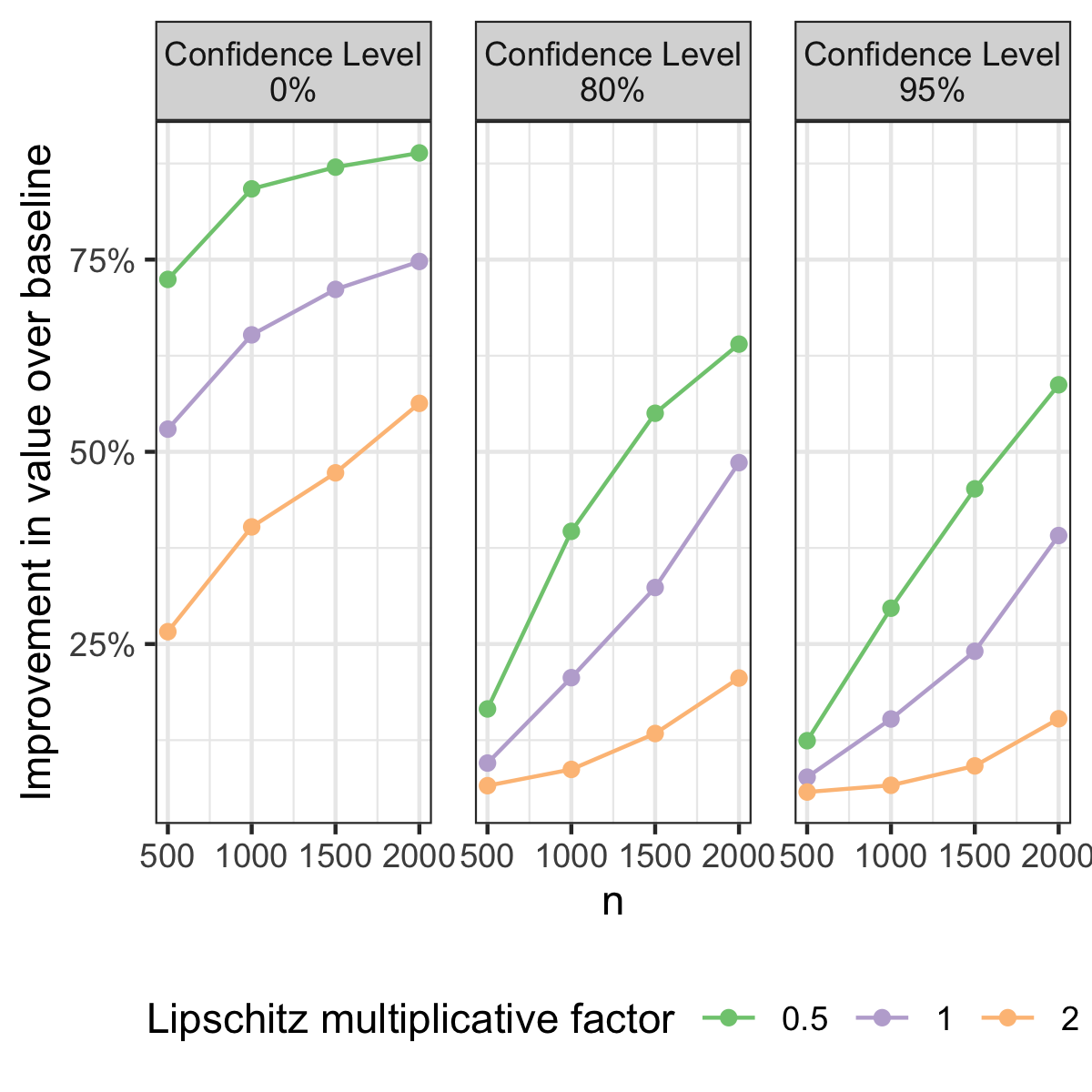
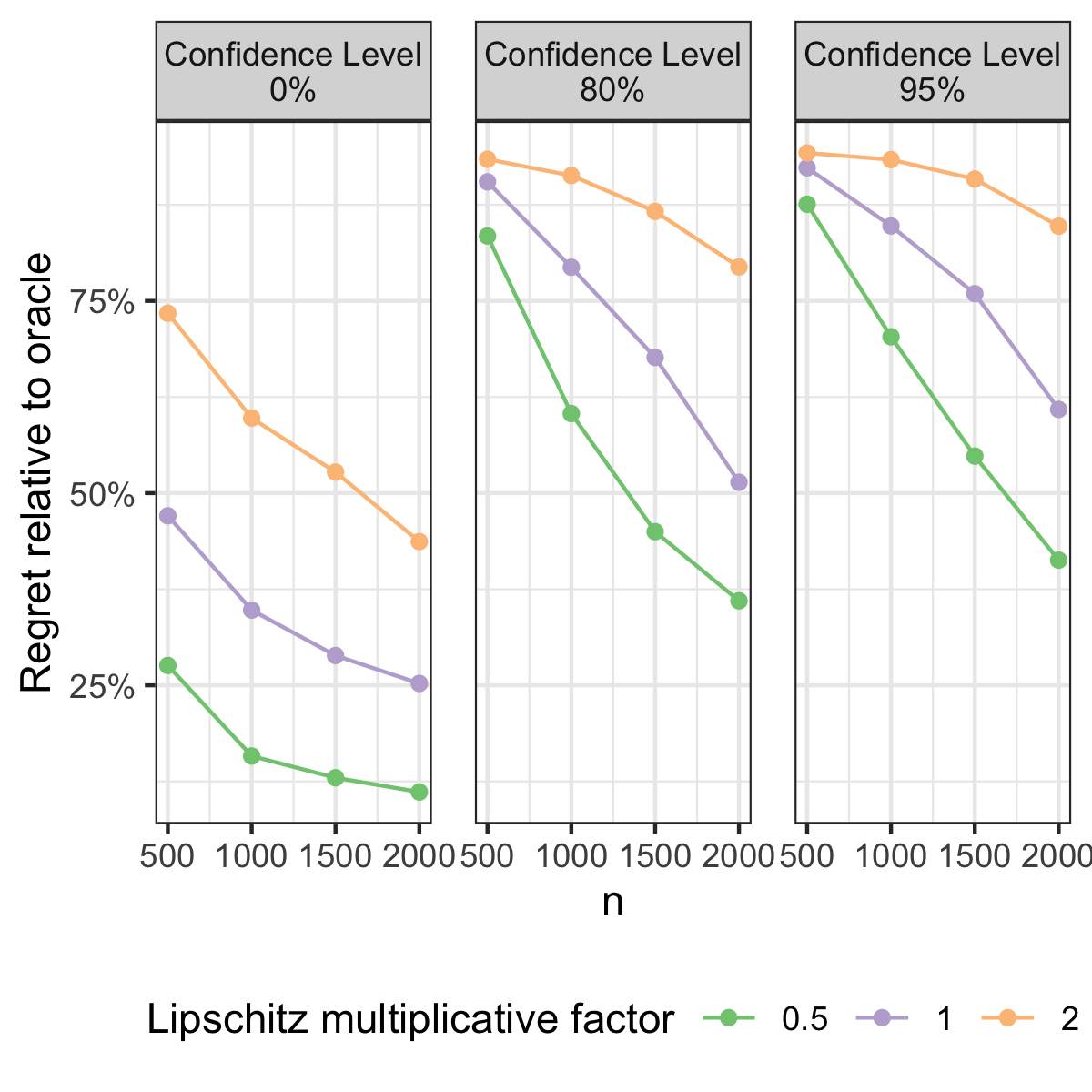
We have a single discrete covariate with 10 levels, , and a binary action so that the action set is . We choose a baseline policy , and set the utility gain to be and the costs to be , so that action 0 is costless and action 1 costs one tenth of the potential utility gain. For each simulation we draw i.i.d. samples uniformly on . Then we draw a smooth model for the expected control potential outcome via random Fourier features. We draw three random vectors: with i.i.d. standard normal elements; with i.i.d. components drawn uniformly on ; and with i.i.d. standard normal elements. Then we set
where the cosine operates element-wise. See Rahimi and Recht (2008) for more discussion on random features. For the potential outcome under treatment, , we add a linear treatment effect on the logit scale:
We then generate the potential outcomes as independent Bernoulli draws with probabilities and , respectively.
With each simulation draw, we consider finding a safe empirical policy by solving Equation (16) under a Lipschitz restriction on the model as in Example 2 and with the threshold policy class in Equation (21). Note that the true model is in fact much smoother than Lipschitz; here we consider using the looser assumption. Following our empirical analysis in Section 7.1, we take the average outcome at each value of , and compute the largest difference in consecutive averages as pilot estimates for the Lipschitz constants and . We then solve Equation (16) using , 1, and 2 times these pilot estimates as the Lipschitz constants, and setting the significance level to 0, 80% and 95%. We additionally compute the oracle threshold policy that uses the true model values and . We do this for sample sizes .
Figure C.1 shows how the empirical safe policy compares to both the baseline policy and the oracle policy in terms of expected utility. First, we see that on average, the empirical safe policy improves over the baseline, no matter the confidence level and the choice of Lipschitz constant. This improvement is larger the less conservative we are, e.g. by choosing a lower confidence level or a smaller Lipschitz constant. Furthermore, as the sample size increases, the utility of the empirical safe policy also increases due to a lower degree of statistical uncertainty. We find similar behavior when comparing to the oracle policy. Less conservative choices lead to lower regret, and the regret decreases with the sample size. Importantly, the regret does not decrease to zero; even when removing all statistical uncertainty the safe policy can still be suboptimal due to the lack of identification.
Appendix D An Additional Figure