A comprehensive revisit of select Galileo/NIMS observations of Europa

Abstract

The Galileo Near Infrared Mapping Spectrometer (NIMS) collected spectra of Europa in the 0.7-5.2 $\micron$ wavelength region, which have been critical to improving our understanding of the surface composition of this moon. However, most of the work done to get constraints on abundances of species like water ice, hydrated sulfuric acid, hydrated salts and oxides have used proxy methods, such as absorption strength of spectral features or fitting a linear mixture of laboratory generated spectra. Such techniques neglect the effect of parameters degenerate with the abundances, such as the average grain-size of particles, or the porosity of the regolith. In this work we revisit three Galileo NIMS spectra, collected from observations of the trailing hemisphere of Europa, and use a Bayesian inference framework, with the Hapke reflectance model, to reassess Europa’s surface composition. Our framework has several quantitative improvements relative to prior analyses: (1) simultaneous inclusion of amorphous and crystalline water ice, sulfuric-acid-octahydrate (SAO), CO${}_{2}$, and SO${}_{2}$; (2) physical parameters like regolith porosity and radiation-induced band-center shift; and (3) tools to quantify confidence in the presence of each species included in the model, constrain their parameters, and explore solution degeneracies. We find that SAO strongly dominates the composition in the spectra considered in this study, while both forms of water ice are detected at varying confidence levels. We find no evidence of either CO${}_{2}$ or SO${}_{2}$ in any of the spectra; we further show through a theoretical analysis that it is highly unlikely that these species are detectable in any 1-2.5 $\micron$ Galileo NIMS data.

1 Introduction

Europa’s young surface and geological features like chaos terrains suggest an active exchange of materials between the surface and subsurface ocean (carr_evidence_1998; moore_surface_2009; kattenhorn_evidence_2014; trumbo_sodium_2019). Accessing the ocean directly to determine its composition will require a sustained program of scientific and technological developments (hand_exploring_2018), and thus our best near-term prospect for determining the ocean composition and constraining Europa’s habitability is to understand its surface composition with available spectra. Europa’s icy surface is, at present, our primary window into the chemistry of the putative subsurface ocean.

Most of our knowledge of Europa’s surface composition comes from reflectance spectroscopy, using ground- and space-based telescopes, as well as instruments onboard spacecraft. The near-infrared reflectance data collected by the Galileo mission, specifically from the Near-Infrared Mapping Spectrometer (carlson_near-infrared_1992), has revolutionized our understanding of Europa’s surface (e.g. mccord_salts_1998; carlson_hydrogen_1999; mccord_hydrated_1999; hansen_amorphous_2004; carlson_distribution_2005; hansen_widespread_2008; dalton_europas_2012; shirley_europas_2016). Spectroscopy in the near-infrared has helped reveal the majority of species identified on Europa’s surface (carlson_europas_2009), including hydrated sulfuric acid (carlson_sulfuric_1999; carlson_distribution_2005), hydrated sulfates (mccord_salts_1998; dalton_linear_2007), chlorinates (fischer_spatially_2015; ligier_vlt/sinfoni_2016) and oxidants (hansen_widespread_2008; hand_keck_2013). Although serendipitous observations of Europa by Juno (filacchione_serendipitous_2019; mishra_bayesian_2021) have provided a new window into this world, the Galileo NIMS dataset still holds great potential to further improve our understanding of Europa’s surface composition, by the application of new, comprehensive methods, as elucidated below.

A standard approach to finding a species in reflectance data is through a spectral fitting analysis (e.g. carlson_distribution_2005; clark_surface_2012). Using a radiative-transfer model, such an analysis also constrains a subset of physical properties like abundances and average grain-sizes. For the NIMS data of Europa, much work has been done with models that fit the data with a linear combination of laboratory spectra of various species (e.g. dalton_linear_2007; dalton_europas_2012). However, this is a rough approximation to the highly non-linear radiative-transfer process through a planetary regolith (e.g. shirley_europas_2016). As a result, linear-mixing type analyses do not allow us to disentangle key properties of the regolith such as average grain-size, porosity, observational geometry parameters, and species abundances, which are highly degenerate with each other.

A more physically motivated alternative is a thorough radiative-transfer model that uses fundamental optical properties of each end-member, alongside parameterizations for physical properties of the regolith (e.g. hapke_2012). Such a model takes into account various inherent degeneracies in the radiative-transfer process and thus yields more conservative estimates of end-member properties, such as abundances and grain-sizes. Physically motivated radiative transfer schemes, such as the Hapke model (hapke_2012), require that optical constants (e.g. refractive indices and extinction coefficients) be measured for several species of interest in the relevant temperature ($\sim 100$ K) and wavelength regime ($\sim 1-5\ \micron$ for most NIMS data). Such laboratory measurements can be challenging, which limits the potential Europan species we can explore using this technique. Thankfully, such optical constants exist for certain key species: amorphous and crystalline water ice at 120 K (grundy_temperature-dependent_1998; mastrapa_optical_2009), CO${}_{2}$ at 179 K (quirico_near-infrared_1997; quirico_composition_1999; sshade), SO${}_{2}$ at 125 K (schmitt_identification_1994; schmitt_optical_1998; sshade) and sulfuric-acid-octahydrate (hereafter SAO) at 77 K (carlson_distribution_2005).

SAO is a major product of the radiolytic sulfur cycle on the trailing hemisphere of Europa (carlson_europas_2009). carlson_distribution_2005 used NIMS data and a simple two-component reflectance model of crystalline ice and SAO to map the distribution of SAO on the leading and trailing hemispheres of Europa, finding concentrations as high as 90% near the trailing hemisphere apex. However, an important form of water ice in the upper-most layers of Europa’s surface may be amorphous ice (e.g hansen_widespread_2008), which was not included in the work by carlson_distribution_2005 due to the unavailability of its optical constants at that time. Since the study of carlson_distribution_2005, a comprehensive database of cryogenic water-ice optical constants, in both amorphous and crystalline forms, was published by mastrapa_optical_2009.

The trace oxides CO${}_{2}$ and SO${}_{2}$ are astrobiologically significant oxidants on Europa’s surface and might play an important role in creating an environment of chemical disequilibrium in its subsurface ocean (e.g chyba_possible_2001; hand_energy_2007). Moreover, CO${}_{2}$ has also been linked to young geological regions on Europa like the chaos terrains (trumbo_h2o2_2019), which indicates a possibly endogenic origin of the carbon that fuels a carbon-cycle on Europa’s surface (carlson_europas_2009; hand2012carbon). Published estimates of CO${}_{2}$ abundances exist for the leading side of Europa, where the 4.25 $\micron$ feature in NIMS spectra (hand_energy_2007) was used to constrain the abundance to be $\sim$ 360 ppm. For SO${}_{2}$, a rough abundance estimate of $\sim 0.2\%$ comes from disk-integrated UV observations of Europa (hendrix_europas_2008; carlson_europas_2009) – although a 4.0 $\micron$ feature has been identified in NIMS spectra (hansen_widespread_2008). Theoretical studies of CO${}_{2}$ and SO${}_{2}$ clathrate formation indicate that the bulk ice-shell of Europa could have an oxidant concentration of up to $\sim 7\%$ (hand_clathrate_2006). It should be noted that while sulfur and its allotropes are also present in significant amounts on the trailing side of Europa – due to the Io-genic bombardement (carlson_europas_2009) – they lack strong features in the NIR wavelength region and hence can be assumed to not affect the NIMS spectra.

To date, only water-ice and SAO have been simultaneously considered in a radiative-transfer based analysis of NIMS data. However, Europa-specific optical constants are now available for amorphous ice, crystalline ice, SAO, CO${}_{2}$, and SO${}_{2}$. Hence, there is an opportunity to model all five species simultaneously in a revised analysis of Galileo NIMS observations of Europa.

In this work we re-analyze a subset of NIMS spectra using the Hapke reflectance model (hapke_2012) in a Bayesian inference framework. Bayesian inference has gained popularity in planetary surface spectroscopic inversion in recent years (e.g. fernando_surface_2013; schmidt_realistic_2015; fernando_martian_2016; lapotre_probabilistic_2017; rampe_sand_2018; belgacem_regional_2020). The goal of this work is to demonstrate a spectroscopic analysis approach rooted in Bayesian inference (mishra_bayesian_2021) that permits several advances over previous analyses of Europan data, specifically: (1) include five species (amorphous ice, crystalline ice, SAO, CO${}_{2}$, and SO${}_{2}$) in a radiative-transfer analysis of Europan spectra; (2) include parameters that account for physical effects, such as radiation-induced band shifts, porosity of the regolith, and calibration uncertainty of the instrument; (3) yield statistical constraints on parameters, including confidence intervals; and (4) provide detection significances for each individual species with a statistical metric via Bayesian model comparisons. The fitting analysis in our approach enables identification of trace species, taking into account their effect on the spectrum over the entire wavelength range, instead of relying on a few sharp features.

We apply this framework to three NIMS spectra of the trailing hemisphere of Europa, spanning 1.0-2.5 $\micron$. These data were available in their reduced form, along with all the observation geometry parameters needed for our analysis, through previous work by carlson_distribution_2005. The data and their properties are described in section 2. Section 3 lays out the details of our analysis framework, including the Hapke reflectance model (section 3.1) and the Bayesian inference methodology (section 3.2). We discuss the results from the application of this framework to the three spectra in section 4, followed by a theoretical study (section LABEL:sec:detectability) to gauge the detectability of CO${}_{2}$ and SO${}_{2}$ as a function of their abundance in synthetic NIMS spectra over the 1.0-2.5 $\micron$ range. We conclude with a discussion (section LABEL:sec:discussion) of our results, placing them in the context of existing knowledge of Europa’s surface composition, before summarizing (section LABEL:sec:conclusions) the key takeaways from our work.

2 Data

During the Galileo spacecraft’s first orbit of Jupiter, the NIMS instrument acquired several spectral maps of Europa, the first being a map of the northern hemisphere in the trailing- side anti-Jupiter region and termed the G1ENNHILAT01A observation. Approximately 300 spectra were obtained in this observation and projected as a point-perspective spectral radiance-factor map. Three types of terrain (highly hydrated, icy, and intermediate) were chosen, for illustration of the diversity in composition, and a single pixel spectrum for each region was extracted and fit using experimentally-derived indices of refraction (carlson_distribution_2005; note the interchange of radiance factor and coefficient therein). This work focuses on those three spectra, which are shown in Figure 1, and will henceforth be referred to as $S1$, $S2$ and $S3$. The locations on Europa’s surface corresponding to these three spectra are shown in Figure 2, and details about the spacecraft observation geometry is shown in Table 1. carlson_distribution_2005 found that $S1$, $S2$ and $S3$ represent a range of compositions of Europa’s trailing hemisphere, from highly hydrated to minimally hydrated. Hence, they also allow us to explore trends in the physical and chemical parameters included in our model across regions of differing water-ice content.

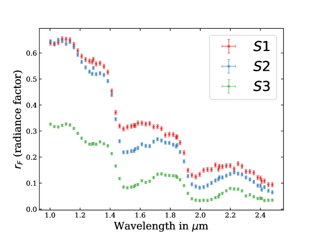
Figure 1: The three Galileo NIMS observations, referred to as $S1$, $S2$ and $S3$, being used in this work. The spectra come from observation G1ENNHILAT01 by Galileo that mapped the trailing hemisphere of Europa. Details for the three spectra are provided in Table 1 and the their locations on Europa’s surface is shown in Figure 2. $S1$, $S2$ and $S3$ also correspond to the bottom, middle and top spectra, respectively, shown in Figure 3 of carlson_distribution_2005.

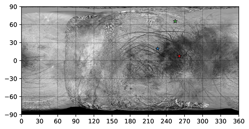
Figure 2: The approximate locations on Europa’s surface, marked as red, blue and green stars, corresponding to spectra $S1$ (7.5$\arcdeg$ N, 261.4$\arcdeg$ W), $S2$ (19.9$\arcdeg$ N, 225.6$\arcdeg$ W) and $S3$ (65.5$\arcdeg$ N, 254.6$\arcdeg$ W) respectively (see Table 1 for details). This map is centered on 180$\arcdeg$ W, where the 0$\arcdeg$ W corresponds to the sub-Jovian longitude. The global base map of Europa was downloaded from USGS ‘Map a Planet’${}^{a}$, derived from Galileo and Voyager images, and is shown in cylindrical projection.

${}^{a}$https://astrocloud.wr.usgs.gov/index.php?view=map2

Table 1: NIMS spectra from the G1ENNHILAT01 observation of Europa being analyzed in this work and referred to as $S1$, $S2$ and $S3$. These spectra are shown in Figure 1.

Spectrum	Line-sample	Latitude	Longitude		Incidence	Emergence		Phase
					angle	angle		angle
S1	32-27	7.5	261.4		24.3	43.8	31.0
S2	45-46	19.9	225.6		25.0	7.0	30.9
S3	20-64	65.5	254.6		67.9	49.1	30.8

Note. — The G1ENNHILAT01 observation approximately spanned latitudes 30$\arcdeg$ S - 90$\arcdeg$ N and longitudes 150$\arcdeg$ W - 300$\arcdeg$ W, with approximate scale of 39 km/pixel (carlson_distribution_2005). Latitude 0$\arcdeg$ and Longitude 0$\arcdeg$ correspond to the sub-Jovian point on Europa’s surface, with longitude increasing positively westward towards the leading hemisphere. $S1$, $S2$ and $S3$ are all from the trailing hemisphere of Europa.

The compositional discriminative power of a spectral analysis method like Bayesian inference depends sensitively on the uncertainties in the data (see section 3 of mishra_bayesian_2021). For most NIMS spectra, including $S1$, $S2$ and $S3$, accurate uncertainties could not be calculated because Galileo’s satellite observations were limited in temporal duration by the relative spacecraft-satellite velocity and by the solar illumination incidence angles. In addition, data transmission to the Earth was severely limited, consequently repeated measurements of a particular region on Europa’s surface were precluded. It is the intrinsic variation among the repeated measurements that informs the uncertainties on the data. Estimates of the uncertainties on data of the kind considered here are usually obtained from repeated measurements of a particular region of interest. Because the spacecraft’s flybys when the data was collected were very short in duration, such repeated measurements could not be taken.

While rough estimates on the SNR (signal-to-noise ratio) of Galileo data in the literature put the number between 5 and 50 (greeley_future_2009), the noise characteristics vary with wavelength and depend on instrumental and external factors that change from observation to observation (carlson_near-infrared_1992). The noise in the NIMS instrument includes thermal noise (which comes from the blackbody IR emission of the interior instrument housing), detector current noise that is approximately proportional to the inverse of the solar spectral irradiance, a small amount of digitization noise, and radiation noise that produces pulses of detector current with widely ranging amplitudes. The observations we are using did not suffer excessive radiation noise, but a small but non-quantifiable amount. We’re assuming we’re working in the photon-noise limited regime, which allows us to measure all the sources of “error” via the scatter they induce on the signal. We obtain estimates of this inherent scatter in each of $S1$, $S2$ and $S3$, caused by a combination of all the factors listed above, by adopting the following process:

1. Assume a SNR of 50 across all wavelength channels.

2. Perform a fitting analysis with a full model (all five species included) and evaluate the best-fit or the maximum-likelihood solution. The details of the analysis framework are discussed in the next section (section 3).

3. Calculate the residuals of this fit to the data.

4. Calculate the standard deviation of these residuals or the SDR.

5. Repeat the steps for SNR of 5.

The larger of the two SDR values, from the SNR=5 and SNR=50 cases, is chosen to be a conservative estimate of the noise in a given spectrum and is assigned as the uncertainty across all channels. This analysis results in data uncertainties of 0.0081, 0.0063, and 0.0047 (in radiance factor units), which correspond to an average SNR (averaged across the wavelength channels) of 39.51, 44.43 and 28.35 for $S1$, $S2$ and $S3$ respectively. These values fall in the range of 5 to 50 that is generally assumed to be the average SNR of NIMS spectra of Europa (greeley_future_2009).

Finally, an important dataset needed for our model are the optical constants for the species considered, which are shown in Figure 3 (sources are mentioned in the figure caption). We use amorphous and crystalline water-ice optical constants at 120 K, similar to carlson_distribution_2005. For SAO, CO${}_{2}$ and SO${}_{2}$, we have selected available optical constants that were derived at temperatures close to the Europan temperature range of 80-130 K (spencer_temperatures_1999). We note that optical constants for the species considered here are temperature dependent, thus both the measured and theoretical reflectance spectra employed in this study will be sensitive to temperature as well (dalton_spectroscopy_2010). Future work that expands on either the species or wavelengths consider here would be best served by additional laboratory-derived optical constants obtained at Europan temperatures.

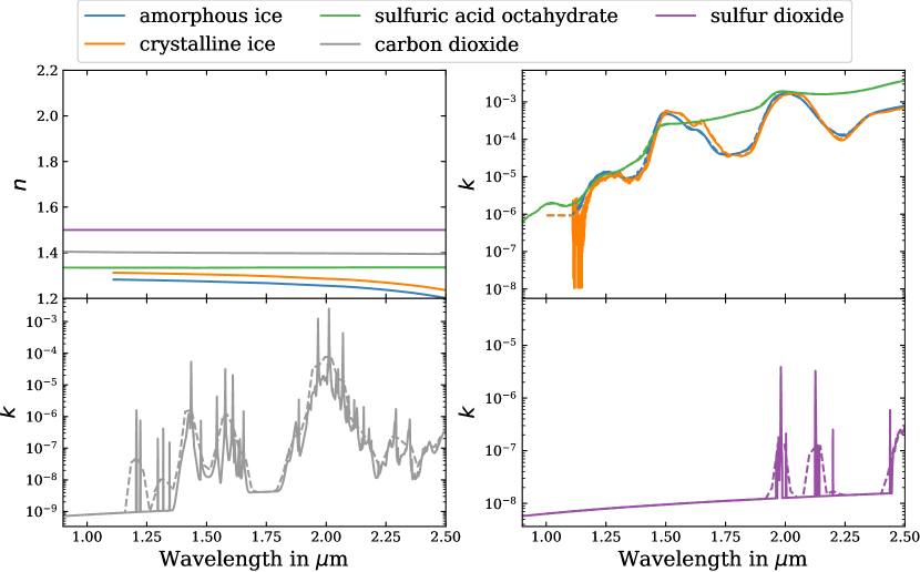
Figure 3: Optical constants $n$ and $k$ of species included in this analysis. Dashed lines in the bottom-left, top-right and bottom-right panels show the $k$ spectra convolved to the NIMS resolution. CO${}_{2}$ and SO${}_{2}$ $k$ spectra have been individually shown in the bottom panels for clarity. Amorphous and crystalline ice optical constants, at 120 K, were published and included in mastrapa_optical_2009; SAO optical constants at 77 K were measured by carlson_distribution_2005; CO${}_{2}$ optical constants, at 179 K, are from quirico_near-infrared_1997; quirico_composition_1999; SO${}_{2}$ optical constants, at 125 K, are from schmitt_identification_1994; schmitt_optical_1998. CO${}_{2}$ and SO${}_{2}$ optical constants are available in the Solid Spectroscopy Hosting Architecture of Databases and Expertise or SSHADE (sshade).

3 Methods

We use a Bayesian inference framework to analyze $S1$, $S2$ and $S3$, which has been described in detail in mishra_bayesian_2021. Briefly, the two major components of this framework are the Forward model and the Bayesian posterior sampling, described in the next two sections. The Bayesian posterior sampling efficiently samples the parameter space we wish to explore, generating millions of instances of Forward model spectra, and selects the samples for which the corresponding model instances fit the data well. From this collection of samples, one can get marginalized posterior distributions of individual parameters, pair-wise 2D distributions of parameters that highlight correlations, and a marginal probability of the model itself, also known as the Bayesian evidence, that is used for model comparison (e.g. trotta_bayesian_2017).

3.1 Forward model

To a good approximation, the bidirectional reflectance of a planetary regolith (hapke_2012) can be written as:

$$r_{F}(\mu,\mu_{0},g,\lambda)=K\dfrac{\omega(\lambda)}{4}\dfrac{\mu_{0}}{(\mu+\mu_{0})}[P(g,\lambda)+H(\omega,\mu/K)H(\omega,\mu_{0}/K)-1]$$ (1)

Here

• $r_{F}$ is the radiance factor, which is the ratio of bidirectional reflectance of a surface to that of a perfectly diffuse surface (Lambertian) illuminated and observed at an incidence angle, $i=0$, relative to the surface normal.

• $\mu$ is the cosine of the emergence angle $e$.

• $\mu_{0}$ is the cosine of the incidence angle $i$.

• $g$ is the phase angle.

• $K$ is the porosity coefficient.

• $\omega$ is the single scattering albedo.

• $P$ is the particle phase function.

• $H$ is the Ambartsumian-Chandrasekhar function that accounts for multiple scattered component of the reflection (chandrasekhar_radiative_1960).

Here, we have ignored parameters related to backscattering and other opposition effects as they become important below small phase angles for the coherent backstatter effect and typically less than a few tens of degrees for the shadow-hiding opposition effect (hapke_opposition_2012; Hapke_2021_opposition), whereas the phase angles of all three NIMS spectra used here are much higher ($\sim 30\degree$, see Table 1). In addition, we ignore the photometric contribution of macroscopic roughness, which Hapke characterizes with a mean topographic slope angle, $\overline{\theta}$. Our available range of photometric geometries for $S1$, $S2$, and $S3$ is too limited to constrain $\overline{\theta}$, which, even at a single phase angle, requires sufficient coverage of incidence and emission angles to characterize the limb-darkening behavior of the surface. Moreover, global average values of $\overline{\theta}$ derived from Voyager and Galileo imaging data vary little from $16^{\circ}$ to $22^{\circ}$ among different works (verbiscer_photometric_2013). At the photometric geometry of the NIMS spectra for S1, S2, and S3, the effects should be small enough to be ignored. However, we note that the detectability of photometric roughness is albedo-dependent such that the measurable values of $\overline{\theta}$ diminish as the surface albedo approaches unity because of multiply-reflected light among topographic surface facets. Since the particle spectral albedos vary with wavelength, it is reasonable to expect that there may be a wavelength-dependent variation in the effects of macroscopic roughness on our spectra. None of our reflectance values approach close enough to unity for this to be a significant concern.

The equations for the single scattering albedo, $\omega$, come from the equivalent-slab approximation (hapke_single-particle_2012). For the phase function $P$, we use a two-parameter Henyey-Greenstein function (henyey_diffuse_1941), which has been shown to be representative of a wide variety of planetary regoliths, including the icy particles on Europa (hapke_single-particle_2012). A detailed description of all the parameters in eq. 1 can be found in the Appendix of mishra_bayesian_2021.

We are also assuming that the regolith in the heavily bombarded and sputtered trailing hemisphere of Europa, where $S1$, $S2$ and $S3$ come from, is well-mixed or ‘churned’ (carlson_europas_2009; shirley_europas_2016). Hence, particles of different species are mixed homogenously together in a intimate mixture. The averaging process in this intimate mixing model is over the individual particle, and $\omega$ and $P$ in Eq. 1 become volume averages of different materials in the mixture:

$$\omega_{mix}=\dfrac{\sum_{j}N_{j}\sigma_{j}Q_{Ej}\omega_{j}}{\sum_{j}N_{j}\sigma_{j}Q_{Ej}}=\dfrac{\sum_{j}f_{j}\sigma_{j}Q_{Ej}\omega_{j}}{\sum_{j}f_{j}\sigma_{j}Q_{Ej}}$$ (2)

$$P_{mix}=\dfrac{\sum_{j}N_{j}\sigma_{j}Q_{Ej}\omega_{j}P_{j}}{\sum_{j}N_{j}\sigma_{j}Q_{Ej}\omega_{j}}=\dfrac{\sum_{j}f_{j}\sigma_{j}Q_{Ej}\omega_{j}P_{j}}{\sum_{j}f_{j}\sigma_{j}Q_{Ej}\omega_{j}}$$ (3)

where for a species of type $j$, $N_{j}$ is the number of particles per unit volume, $\sigma_{j}(=\pi D^{2}/4)$ is the cross-sectional area, $Q_{E,j}$ is the volume average extinction efficiency, $\omega_{j}$ is the the single scattering albedo, $P_{j}$ is the phase function, and $f_{j}$ is the number density fraction, equivalent to $N_{j}/\sum N_{j}$. For more details about the mixing equation parameters, please refer to section 2.2.2 of mishra_bayesian_2021.

3.2 Bayesian posterior sampling

The parameters we are fitting for, which define the parameter space are:

• log${}_{10}$($X_{i}$), where $X_{i}$ is the abundance (or number density fraction) of each species

• log${}_{10}$($D_{i}$), where $D_{i}$ is the grain-size of each species

• filling factor $\phi$, which is the volume fraction occupied by particles, equivalent to 1 - (porosity of the regolith). $\phi$ is related to the porosity coefficient $K$ in eq. 1 through the relation $K=-ln(1-1.209\phi^{2/3})/(1.209\phi^{2/3})$.

• a multiplicative factor $c$ for the model spectrum. In the 1-2.5 $\micron$ region, the absolute calibration of the NIMS instrument, or the accuracy of its measurements, is uncertain to around $\pm 10\%$ (carlson_near-infrared_1992; carlson_distribution_2005).

• a wavelength-shift parameter $\Delta_{wav}$, to shift the absorption band centers of the model spectrum by $\Delta_{wav}$ , mimicking radiation induced shifts.

We have included the $\Delta_{wav}$ parameter because Europa’s trailing hemisphere spectra, like $S1$, $S2$ and $S3$, have water absorption-band centers that are shifted to slightly shorter wavelengths, by about tens of nanometers. This is a known effect of particle irradiation on fundamental absorption bands of hydrates, sulfates and silicates (e.g. dybwad_radiation_1971; nash_ios_1977). For Europa specifically, it has been emphasized that comparisons of lab and numerically modelled spectra to Europa spectra must allow for the radiation-induced shifts of hydrate bands, so as to not bias our inference of the chemical composition from the spectra (carlson_europas_2009). One way to circumvent the problem would be to discard the data points near band-edges (e.g carlson_distribution_2005). However, we find that our wavelength-shift parameter $\Delta_{wav}$ works sufficiently well and results in excellent fit to the data. An example is shown in Figure 4, where $S1$ is fit with a model with and without the $\Delta_{wav}$ parameter, with a much superior fit in the latter case. Moreover, measuring this wavelength shift for different spectra can also inform us about trends in the level of irradiation experienced by the regoliths corresponding to the spectra. Hence, we include this parameter in all subsequent analysis.

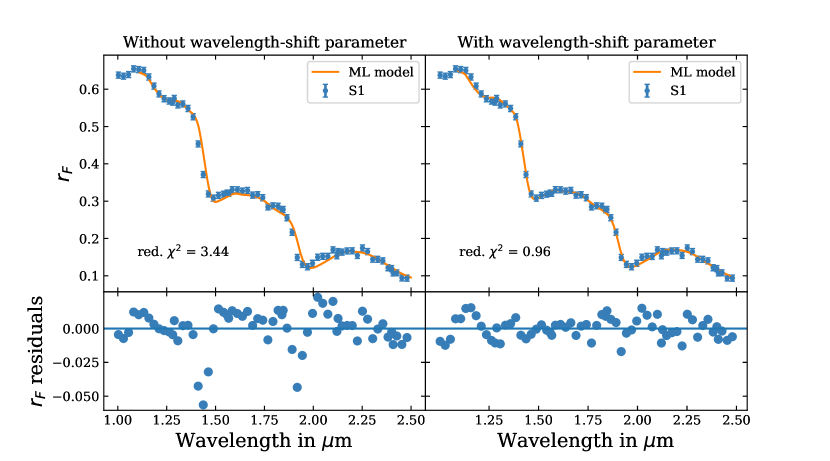
Figure 4: Best-fit or maximum likelihood solutions of a SAO and amorphous ice model fit to $S1$ (blue points). The left panel shows the solution (orange) for the case where a wavelength-shift parameter is not included, while the right panel shows the solution (orange) for the case where that parameter is included (this turns out to be the preferred model for $S1$ as shown in section 4). In the left panel, the model is slightly shifted to longer wavelengths as compared to the data, around the band-edges near 1.4 and 1.9 $\micron$. The reduced $\chi^{2}$ values of the fits are also noted, which illustrate that the fit in the right panel is better.

To sample this multi-dimensional parameter space, we use the nested sampling algorithm (skilling_nested_2006). Specifically, we employ the Python implementation called dynesty, which implements dynamic nested sampling (higson_dynamic_2019), a more computationally accurate version of the standard nested sampling algorithm. Schematically, the iterative parameter exploration by nested sampling proceeds as follows:

1. A random instance of a set of parameters or a parameter vector is drawn from the parameter space, defined by the prior distribution function. For abundances, we use a Dirichlet prior (e.g. benneke_atmospheric_2012; lapotre_probabilistic_2017), which ensures that the abundance parameters being sampled satisfy the constraint that they should sum up to 1. For the rest of the parameters, which do not have any such constraints, we use a uniform distribution, which is relatively uninformative (as compared to a Gaussian prior, for example), leading the data to drive the solution. The prior function also serves the purpose of defining the boundary of the parameter space to explore. Table 2 lists all the free parameters, their prior function type and bounds.

2. Using these parameters, with the optical constants of the component species and the observation geometry parameters as the main inputs, the forward model (section 3.1) generates a model spectrum and then convolves it with the instrument response function (or bins it to the instrument’s resolution) to produce simulated data points. Each NIMS channel has a triangular response function (carlson_near-infrared_1992; carlson_distribution_2005), spanning the channel-width of $\sim 0.026\ \micron$.

3. These predicted data points are compared with observed data points to compute the posterior probability of this particular instance of parameters, defined by the Bayes’ theorem as follows:

   $$p(\theta_{j}|d,M)=\dfrac{p(d|\theta_{j},M)p(\theta_{j}|M)}{\int p(d|\theta_{j},M)p(\theta_{j}|M)d\theta_{j}}\equiv\dfrac{\mathcal{L}(d|\theta_{j},M)\pi(\theta_{j}|M)}{\mathcal{Z}(d|M)}$$ (4)

   where $\mathcal{L}(d|\theta,M_{i})$ is the likelihood probability function, $\pi$ is the prior, $\mathcal{Z}$ is the Bayesian evidence and $p(\theta|d,M)$ is the posterior probability function. Since we assume the errors on our data to be Gaussian and independent, the likelihood function is also a Gaussian equal to

   $$\mathcal{L}(d|\theta,M_{i})={\displaystyle\prod^{N_{obs}}_{k=1}}\dfrac{1}{\sqrt{2\pi\sigma_{k}^{2}}}\textrm{exp}\Big{(}-\dfrac{\chi^{2}}{2}\Big{)}$$ (5)

   where $N_{obs}$ is the number of observed data points (i.e., number of wavelength channels/data points in the observed spectrum), $\chi^{2}$ is the familiar goodness-of-fit metric, and $\sigma$ is the standard deviation.

4. The posterior probability decides whether this particular parameter set is saved or selected and, in turn, informs the choice of the next parameter set as well. Details about this process/algorithm can be found in higson_dynamic_2019.

Table 2: The priors used for all model parameters in our fitting analysis

Parameter	Description	Prior	Range
$f_{i}$	Number-density fraction or abundance	Dirichlet	10${}^{-3.0}$ to 1
$D_{i}$	Average grain diameter (microns)	log-uniform	10 to 1000
$\phi$	filling factor	uniform	0.01 to 0.52
$c$	NIMS calibration uncertainty parameter	uniform	0.7 to 1.1
$\Delta_{wav}$	wavelength-shift parameter ($\mu$m)	uniform	-0.1 to 0.1

Note. — $\phi$’s lower limit has been set to 0.01 because $K$, which is the model parameter dependent on $\phi$ (see eq. 1), plateaus at a value of 1 for $\phi\lesssim 0.01$. The upper limit of 0.52 comes from hapke_bidirectional_2008 where it is described as a critical value above which the medium is too tightly packed, such that coherent effects become important and diffraction can’t be ignored.

After this process converges, the final set of samples can be marginalized to get individual or pair-wise parameter distributions. Another useful quantity that the nested sampling process returns is the Bayesian evidence of the model or $\mathcal{Z}$ (eq. 4), which is discussed in the next section. It quantifies the probability of a model given the data, integrated over the entire parameter space (eq. 4). Hence, two models can be readily compared using $\mathcal{Z}$, in a process called Bayesian model comparison. We adapt this into a nested Bayesian model comparison process, where we compare the evidence for a model with all species (the full model) with models where each species is removed one at a time. Assuming no a priori preference of either the full model or the model without species X, if the Bayesian evidence is higher for the latter, we conclude that X is not needed to explain the data and hence there is no evidence for it. This process helps us select the simplest model, i.e., with the fewest number of species, compatible with the observations. The comparisons are also used to quantify the confidence in the presence of each species remaining in the simplest model, through the $\sigma$-significance metric (see section 2.2.3 of mishra_bayesian_2021 for a full description of statistical aspects of the Bayesian inference methodology). As per empirically calibrated evidence thresholds known as Jeffrey’s scale (jeffreys_1939), a detection significance exceeding around 2.1$\sigma$, 2.7$\sigma$ and 3.6$\sigma$ levels are referred to as ‘weak’, ‘moderate’ and ‘strong’ evidence respectively. We use these metrics to guide our interpretation of our model results.

Over the course of analyzing $S1$, $S2$ and $S3$, we performed around 25 Bayesian inference analyses with models containing different combinations of the five species - amorphous ice, crystalline ice, SAO, CO${}_{2}$ and SO${}_{2}$. A full-model analysis (with all the five species) amounts to 12 free parameters and computes $\sim 4\ \textrm{x}\ 10^{5}$ model spectra. Using this methodology, for each of the three spectra, we now proceed to describe the detection significance of all five species, the simplest model that best explains the spectrum, and the constraints on the parameters of that model.

4 Results

The results for the nested model comparisons performed for $S1$, $S2$ and $S3$ are shown in Table 3. For each spectrum, we first perform a Bayesian inference analysis with a full model, i.e., with all five species - amorphous ice, crystalline ice, SAO, CO${}_{2}$ and SO${}_{2}$. We then remove each species one at a time, and rerun the analysis with these alternative models. Comparing each of their results against the reference model with all five species, we can quantify the evidence for the presence of each species. The retrieved parameter constraints for the models with highest evidence (i.e., the simplest models that explain the data) are shown in Table 4.

Table 3: Results of nested model comparisons for $S1$, $S2$ and $S3$

	$S1$		$S2$		$S3$
Model	ln($\mathcal{Z}_{i}$)	$\chi^{2}_{r,min}$	ln($\mathcal{Z}_{i}$)	$\chi^{2}_{r,min}$	ln($\mathcal{Z}_{i}$)	$\chi^{2}_{r,min}$
All species (ref.)	200.11	1.03	210.831	1.02	236.85	0.73
No SAO	-2453.90 ($>30\sigma$)	99.12	-2523.39 ($>30\sigma$)	102.17	-423.48 ($>30\sigma$)	25.22
No amorphous ice	198.45 (2.4$\sigma$)	1.04	211.01 (N.A.)	1.1	232.67 ($3.36\sigma$)	0.96
No crystalline ice	200.87 (N.A.)	0.99	194.96 ($5.9\sigma$)	1.69	227.28 ($4.76\sigma$)	1.17
No CO${}_{2}$	200.48 (N.A.)	0.99	212.17 (N.A.)	0.98	238.21 (N.A.)	0.70
No SO${}_{2}$	200.55 (N.A)	1.02	212.36 (N.A)	0.98	237.2 (N.A.)	0.71

Note. — For each of the three spectra, $S1$, $S2$ and $S3$, the Bayesian evidence ln($\mathcal{Z}_{i}$) and the minimum reduced chi-squared $\chi^{2}_{r,min}$, i.e, chi-squared of the maximum-likelihood solution are listed for all models. The ‘All species’ model is the reference model to compare to and contains amorphous water-ice, crystalline water-ice, SAO, CO${}_{2}$ and SO${}_{2}$ . The other four alternative models are each without one of the five species as specified. In brackets next to the ln($\mathcal{Z}_{i}$) values, an $n$-$\sigma$ detection indicates the degree of preference for the reference model over the alternative model, which can also be interpreted as the significance of detection of the species excluded from the alternative model. ‘N.A.’ indicates that no evidence for the particular species has been found.

Table 4: Derived parameter values, along with the 1-$\sigma$ upper and lower bounds (68% confidence intervals), for models with highest evidence for $S1$, $S2$ and $S3$. The parameters are described in Table 2. The subscripts ‘sao’, ‘am’ and ‘cr’ stand for sulfuric-acid-octahydrate (SAO), amorphous ice and crystalline ice, respectively. The values in the brackets are the exponentiated versions of the logarithmic results.

Parameter	$S1$	$S2$	$S3$
log${}_{10}f_{sao}$ ($f_{sao}$)	-0.0599${}^{+0.0348}_{-0.0942}$ (0.8711${}^{+0.0727}_{-0.1698}$)	-0.0010${}^{+0.0003}_{-0.0005}$ (0.9976${}^{+0.0007}_{-0.0012}$)	-0.1478${}^{+0.0771}_{-0.1136}$ (0.7115${}^{+0.1382}_{-0.1638}$)
log${}_{10}D_{sao}$ ($D_{sao}$)	1.6254${}^{+0.0576}_{-0.0502}$ (42.2071${}^{+5.9857}_{-4.6100}$)	1.6530${}^{+0.0301}_{-0.0312}($44.9820${}^{+3.2296}_{-3.1217}$)	1.9905${}^{+0.0497}_{-0.0506}$ (97.8381${}^{+11.8737}_{-10.7525}$)
log${}_{10}f_{am}$ ($f_{am}$)	-0.8897${}^{+0.3649}_{-0.3605}$ (0.1289${}^{+0.1698}_{-0.0727}$)	-	-0.5456${}^{+0.1973}_{-0.2870}$ (0.2847${}^{+0.1637}_{-0.1377}$)
log${}_{10}D_{am}$ ($D_{am}$)	1.6919${}^{+0.1175}_{-0.1291}$ (49.1912${}^{+15.2787}_{-12.6505}$)	-	2.0233${}^{+0.1065}_{-0.1232}$ (105.5145${}^{+29.3287}_{-26.0577}$)
log${}_{10}f_{cr}$ ($f_{cr}$)	-	-2.6273${}^{+0.1822}_{-0.1643}$ (0.0024${}^{+0.0012}_{-0.0007}$)	-2.4494${}^{+0.1003}_{-0.0803}$ (0.0036${}^{+0.0009}_{-0.0006}$)
log${}_{10}D_{cr}$ ($D_{cr}$)	-	2.5826${}^{+0.0808}_{-0.0887}$ (382.4395${}^{+78.1922}_{-70.6589}$)	2.9634${}^{+0.0267}_{-0.0484}$ (919.1472${}^{+58.2593}_{-96.8802}$)
$\phi$	0.1511${}^{+0.0771}_{-0.0669}$	0.1883${}^{+0.0631}_{-0.0613}$	0.0319${}^{+0.0357}_{-0.0161}$
$c$	0.7898${}^{+0.0034}_{-0.0034}$	0.8029${}^{+0.0049}_{-0.0055}$	0.9887${}^{+0.0080}_{-0.0095}$
$\Delta_{wav}$	-0.0198${}^{+0.0015}_{-0.0016}$	-0.0098${}^{+0.0010}_{-0.0010}$	-0.0043${}^{+0.0015}_{-0.0015}$

Note. — The units for $D_{i}$ are microns. A ‘-’ indicates that the species was not part of the preferred model. CO${}_{2}$ and SO${}_{2}$ have not been included in this table as neither of them were detected in any of the three spectra.