Treatment Effects in Market Equilibrium

Abstract

When randomized trials are run in a marketplace equilibriated by prices, interference arises. To analyze this, we build a stochastic model of treatment effects in equilibrium. We characterize the average direct (ADE) and indirect treatment effect (AIE) asymptotically. A standard RCT can consistently estimate the ADE, but confidence intervals and AIE estimation require price elasticity estimates, which we provide using a novel experimental design. We define heterogeneous treatment effects and derive an optimal targeting rule that meets an equilibrium stability condition. We illustrate our results using a freelance labor market simulation and data from a cash transfer experiment.

Keywords: Equilibrium Effects, Experimental Design, Interference

1 Introduction

Modern computational infrastructure has enabled an enormous growth of randomized trials on websites and mobile applications (Kohavi et al. 2020). On many online platforms, interactions between individuals occur as they buy and sell items at the prevailing market prices. The goal of running a standard randomized control trial (RCT), where treatment is assigned with constant probability to all individuals, is often to evaluate the impact of a new policy on some outcome of interest. The standard analysis of treatment effects in a randomized trial relies on an assumption that the treatment status of one individual does not affect the outcomes of other individuals (Fisher 1935, Banerjee & Duflo 2011, Imbens & Rubin 2015), also known as the Stable Unit Treatment Value Assumption (SUTVA). When a randomized trial affects supply or demand, and market prices affect the outcome of interest, then general equilibrium effects lead to a violation of SUTVA, and measurements of the Average Treatment Effect (ATE) do not correspond to a meaningful measure of policy impact (Heckman et al. 1998).

A primary goal of this paper is to provide a framework for the analysis of randomized trials in an equilibrium setting without relying on strong parametric, distributional, or homogeneity assumptions. We integrate a price equilibrium into a stochastic model of treatment effects under interference. We use it to provide asymptotic results for various definitions of policy-relevant average and conditional average treatment effects, and to design new forms of randomized trials and targeting rules. In the process, we overcome a variety of challenges unaddressed by the existing literature on treatment effects under dense patterns of interference, including providing asymptotically exact confidence intervals for the indirect effect, and proposing general definitions of conditional estimands that can be used to construct targeting rules.

There is existing work that addresses interference by clustering units at a higher level at which SUTVA holds (Baird et al. 2018, Hudgens & Halloran 2008). In the market context, this involves finding clusters of buyers and sellers who trade only within the cluster and not across clusters. However, if a marketplace is very connected, finding a good clustering may not be feasible. Furthermore, clustering can be costly, both because it reduces power (Abadie et al. 2017) and because cluster-level designs require modifying the equilibrium in different clusters. In this paper, we focus on settings where clustering is not desirable, so that the solution must rely on unit-level randomized experimentation only. This approach results in increased power, but comes at a cost of making assumptions based on ex-ante knowledge about the structure of the market equilibrium.

Structural modeling is used in a variety of fields to analyze the effects of policies when individuals interact with one another in economic environments (Heckman et al. 1998, Duflo 2004, Abbring & Heckman 2007). Some structural models are population-level and are designed for theoretical analysis, as in Johnson (1980). Others are designed for estimating demand systems from observational data by imposing exclusion restrictions or parametric assumptions; see Ackerberg et al. (2007), Matzkin (2015), Berry et al. (1995), Berry & Haile (2021). Compared to observational data that is often at an aggregate level, experiments can be used to collect individual-level data that are much richer. As suggested in Manski (1993), collecting richer data is helpful for analyzing endogenous social effects without imposing strict assumptions on the data generating process. We build a non-parametric structural model that is designed for treatment effect inference using individual-level data from randomized experiments. Our model builds connections between the non-parametric program evaluation literature and the modeling-based approaches that have traditionally been used to analyze equilibrium effects of policies. When marketplace effects are removed, it reduces to a standard Neyman-Rubin potential outcomes model (Imbens & Rubin 2015). We are able to derive estimators, standard errors and targeted policies in equilibrium that are robust to a variety of modeling choices and can be compared directly to related results in the causal inference literature.

The starting point for our model is the potential outcomes framework that allows for cross-unit interference (Hudgens & Halloran 2008, Manski 2013, Aronow & Samii 2017). We assume that each individual’s production and consumption choices are determined by latent supply and demand curves (Angrist et al. 2000, Heckman & Vytlacil 2005). Units interact via a marketplace modeled as a classical multiple goods economy in general equilibrium, where individuals make choices on production and consumption based on their own private information as well as their expectations of what the market price equilibrium will be (Walras 1900, Mas-Colell et al. 1995). Our two main non-parametric structural assumptions are that prices equalize latent supply and demand, and the potential outcomes for each individual depend only on their own treatment and market prices. Under this structure, we show that interference is restricted in that it operates only through the $J$-dimensional equilibrium price. That is, equilibrium prices induce an exposure mapping in the sense of Manski (2013) and Aronow & Samii (2017). When individual supply, demand and outcomes are stochastic, we show that the random equilibrium price that arises in finite samples converges to a fixed and unique price in the limit as the number of suppliers and consumers grows. We use this mean-field limit to characterize the asymptotic behavior of treatment effects.

Under interference, a meaningful policy-relevant counterfactual is the Global Treatment Effect (GTE), which is the average effect of treating all individuals in the sample compared to treating no individuals in the sample. Hu et al. (2022) show that under any pattern of interference, the sum of the average direct and indirect effects of a binary treatment is a first-order approximation to the GTE. Thus, we start by analyzing the average direct and indirect effects of a binary treatment in equilibrium (Halloran & Struchiner 1995, Hu et al. 2022, Sävje et al. 2021). We show that the direct and indirect effects of a binary treatment converge to simple and interpretable mean-field limits in large samples. The direct effect converges to the difference in expected outcomes for treated and control individuals, holding market prices fixed. The indirect effect converges to the product of the effect of the treatment on excess demand, the derivative of expected outcomes with respect to prices, and the inverse of the sensitivity of excess demand with respect to prices.

The direct effect of the treatment can be consistently estimated using a Horvitz-Thompson estimator and data from a traditional RCT, as shown in Sävje et al. (2021). We also provide a Central Limit Theorem for the Horvitz-Thompson estimator and characterize the asymptotic variance explicitly. Confidence intervals built for the direct effect using a standard RCT approach that ignores equilibrium effects are not exact. In order to perform asymptotically exact inference for the direct effect and to consistently estimate the indirect effect, which is the missing component of the policy counterfactual, estimates of price elasticities are required.

We propose an augmented unit-level randomized experiment that adds small price perturbations to a traditional Bernoulli randomized experiment. This is feasible, for example, in online marketplaces, where there are often fees for buyers and sellers that can be perturbed randomly. We show that adding small price perturbations does not affect the limiting equilibrium of the system. In previous work that characterizes the indirect effect under dense patterns of interference, estimators for the variance of the indirect effect were not available (Li & Wager 2022, Sävje et al. 2021). Under this augmented randomized experiment, we provide a central limit theorem and characterize the asymptotic variance for the indirect effect, and show that consistent estimators for the direct and indirect effect and their asymptotic variances are available.

Given that the model we’ve been using so far allows for unrestricted heterogeneity across agents, it is also interesting to see whether we can estimate how treatment effects vary with pre-treatment characteristics—and exploit this heterogeneity to learn improved policies. In Section 4, we analyze heterogeneous effects and optimal treatment rules under equilibrium interference. In settings where SUTVA holds, there is a large literature on characterizing heterogeneity in treatment effects and treatment targeting (Manski 2004, Athey & Imbens 2016, Wager & Athey 2018, Van der Weele et al. 2019). Optimal policy in this setting depends on the sign and magnitude of the conditional average treatment effect (CATE) (Manski 2004). However, in the presence of interference, the CATE alone does not explain who should be treated to optimize outcomes; and in fact the standard definition of the CATE is ill-specified (since it relies on SUTVA). Given this background, our first contribution is to define conditional estimands under general patterns of interference that connect to a meaningful policy counterfactual and are useful in defining optimal targeting rules. We propose the conditional average direct effect (CADE), which is the expected effect of changing the treatment of an individual with covariate $x$ on their own outcomes, and the conditional average indirect effect (CAIE), which is the expected effect of changing the treatment of an individual with covariate $x$ on everyone else’s outcomes. We show that the sum of the CADE and the CAIE, scaled appropriately, is equal to the expected increase in average outcomes for a marginal increase in the treatment probability of an individual with covariate $x$. Just as the ADE is equal to the ATE when interference is removed, the CADE is equal to the CATE when interference is removed. Under the model of Section 2, the CADE and the CAIE converge to mean-field limits, that depend on a combination of average price elasticities and conditional average direct effects of the treatment on outcomes and excess demand.

The sum of the CADE and the CAIE can be used to estimate the optimal unconstrained treatment rule using the experiment of Section 3, which includes price perturbations. The structure of the conditional estimands under equilibrium interference, however, is such that it is possible to use data from a standard RCT, without price elasticity estimates, to estimate the optimal targeting rule when it is constrained to have the same equilibrium effect as the RCT. The optimal treatment rule takes the form of a hyperplane in the space of the conditional average direct effects of the treatment on both outcomes and excess demand. The gain of this targeting rule over a uniform rule is estimable using a data splitting approach. This provides a metric of heterogeneity under equilibrium interference that is estimable using data from a standard RCT and readily available software for CATE estimation.

Finally, in Section 5, we demonstrate the consistency and coverage properties of our treatment effect and variance estimators using simulations of a marketplace with a supply-side nudge intervention that affect individuals directly and indirectly through market prices. We also include an empirical illustration of the equilibrium-stable targeting rule using data from a large cash transfer experiment in Mexico published by Gertler et al. (2012). The targeting rule results in significantly higher estimated average agricultural income for households in the data sample, when average land usage under the targeting policy is constrained to be equal to that of the uniform policy from the original RCT.

1.1 Related Work

As discussed in the introduction, most existing work on treatment effect estimation under equilibrium effects (or other types of interference) adopts a standard randomization-based framework, where SUTVA holds for higher-level clusters of units (Baird et al. 2018, Basse et al. 2019, Hudgens & Halloran 2008, Karrer et al. 2021, Liu & Hudgens 2014, Tchetgen & VanderWeele 2012). Another related approach is the network interference model, which posits that interference operates along a network and the connections between units are sparse (Athey et al. 2018, Leung 2020, Sävje et al. 2021). The sparsity of connections then enables randomization-based methods for studying cluster-randomized experiments to be extended to this setting. In our setting, however, the interference pattern produced by marketplace price effects is dense and simultaneously affects all units, so cluster- or sparsity-based methods are not applicable.

There is very little available work on targeting treatments under interference. One notable exception is Viviano (2019), who estimates treatment allocation rules in a network interference model. However, his results rely on sparsity of the network structure and so they are not directly comparable to ours. Furthermore, Viviano (2019) proceeds via direct empirical welfare maximization over a restricted policy class as in, e.g., Kitagawa & Tetenov (2018) and Athey & Wager (2021), and so he doesn’t define CATE-like quantities in his model. We also note recent work by Sahoo & Wager (2022) on policy learning in a model where agents can strategically modify covariates used for treatment assignment and the policymaker has a budget constraint. They show that this setting results in a type of interference, and consider methods that account for this. Again, however, their approach relies on a form of direct welfare maximization and they do not consider CATE-like quantities.

We use total differentiation of the mean-field equilibrium condition to characterize the sensitivity of the mean-field equilibrium price with respect to the treatment in terms of estimable elasticities and treatment effects. In a theoretical analysis, Johnson (1980) uses a low-skilled labor market-clearing condition to characterize the effects of immigration on domestic employment. Similar techniques are used to express policy effects in terms of estimable elasticities in a variety of non-equilibrium settings; see Chetty (2009). In this paper, we start with a non-parametric stochastic model of a finite-sample marketplace, which has an equilibrium condition that is not differentiable or amenable to traditional techniques. We show that average effects in this stochastic model have limits which correspond to population quantities that are amenable to “sufficient statistics”-type analysis. This leads to valid inference strategies and an analysis of heterogeneity that are not available when working with a population model directly.

In empirical work with observational data, instrumental variables approaches have been used in both parametric and non-parametric settings to estimate price elasticities or a weighted average of elasticities (Angrist et al. 1996, Berry & Haile 2021). Angrist & Krueger (2001) reviews IV approaches and their relation to causal inference for observational data. There is a variety of more recent work on using IV approaches to identify causal effects in a variety of settings beyond a price equilibrium, an incomplete list includes Heckman & Pinto (2018), Chesher & Rosen (2017), and Vazquez-Bare (2022). In our paper, we require an estimate of price elasticities to perform inference on average treatment effects. The price elasticities required are an average over all individuals in the market, rather than a weighted average as in the Local Average Treatment Effect literature. Our introduction of price perturbations can be interpreted as creating an ideal instrumental variable for the market price, where by construction everyone in the market is a complier so that the required price elasticities are estimated exactly. In settings where it is not possible to randomize individual-level fees, then with additional assumptions, a more structured IV-based approach could be used instead for estimating elasticities. Given there is already a large existing literature on price elasticity estimation in settings where there is more limited variation available in the data, we do not explore this direction further in this paper.

In development economics, there is concern that interventions can have general equilibrium effects that have a meaningful welfare impact but are not captured by standard randomized control trials. Banerjee et al. (2021) uses a cluster-randomized experiment to show that, in certain remote villages, in-kind food subsidies can have an impact of market prices. Other recent work on general equilibrium effects in development settings includes the structural approach of Duflo (2004) and the cluster-based approach of Muralidharan et al. (2017) and Egger et al. (2022). Our results suggest that it is possible for researchers to evaluate general equilibrium effects without running a cluster-randomized experiment, if the market of interest has a large number of buyers and sellers and convincing estimates of relevant price elasticities are available.

Reducing policy effects to estimable parameters without fully specifying a model has a long history in economics, see Marschak (1953) and Heckman (2008). Wolf (2019) uses a semi-structural approach to decompose the effect of macroeconomic shocks into partial equilibrium effects and general equilibrium effects (e.g., price effects), but uses time series methods to estimate the price effects, in contrast to the unit-level approach presented in this paper. Heckman et al. (1998) uses a calibrated overlapping generations model to estimate equilibrium treatment effects in a model of school choice in a labor market equilibrium. Neilson et al. (2019) uses a randomized control trial to estimate the direct effect of information provision on school choice but simulates a fully parametric structural model to evaluate equilibrium effects of the treatment. Compared to this existing work, our approach is unique in that it takes a fully non-parametric approach to analyzing general equilibrium effects based on unit-level experiments that reduces to the standard Neyman-Rubin potential outcomes framework when equilibrium effects are removed.

Our use of latent choice models—specifically latent supply and demand curves—to construct potential outcomes builds on a long tradition in econometrics going back to the work of Roy (1951) and Heckman (1979) on endogenous selection models. Heckman & Vytlacil (2005) offer a more recent synthesis line of work, and use it to derive instrumental variable estimators for a number of policy-relevant variables. The specific latent choice model used here is most closely related to that used in Angrist et al. (2000), who used it to characterize the behavior of two-stage least squares estimators when used to estimate supply and demand elasticities.

Our approach relies on positing a stochastic model where the types of individuals are generated by an underlying probability distribution, and analyzing effects in the limit as the number of individuals in the model grows large. This approach is inspired by mean-field modeling. There is a large literature that uses the mean-field limit to study large-scale stochastic systems in operations research, engineering and physics (Mézard et al. 1987, Tsitsiklis & Xu 2013, Vvedenskaya et al. 1996). Also related are economic models where players respond to the average behavior in the system (Weintraub et al. 2008, Hopenhayn 1992, Krusell & Smith 1998).

We also note a handful of recent papers that leverage stochastic modeling and mean-field type results in a causal inference setting. Johari et al. (2020) use a mean-field model to examine the benefits of a two-sided randomization design in two-sided market platforms and quantify the bias due to interference between market participants. Li & Wager (2022) study large sample results for treatment effect estimation under network interference, where units are placed at vertices of an “exposure graph” and a unit’s potential outcome may depend on another unit’s treatment if and only if they are connected by an edge in the graph; they further posit that the exposure graph is randomly generated from a graphon model. Finally, Wager & Xu (2021) consider a model of a marketplace that matches exogenous demand to endogenous supply, with interference via supply cannibalization. They propose using zero-mean perturbations to estimate a revenue gradient and optimize a continuous decision variable dynamically. Our work also uses zero-mean perturbations as part of a unit-level experiment, but is otherwise distinct, given our focus is on treatment effects of a binary intervention in a general price equilibrium.

2 Treatment Effects under Market Interference

2.1 Treatment Effects Under Interference

We first review a definition of treatment effects in the potential outcomes framework when individuals are sampled from a population, which will allow us to model general interference patterns between units. Consider a system comprised of $i=1,\ldots,n$ individuals who are sampled independently from a population, where individual $i$ has features $X_{i}\in\mathcal{X}$. We will work in a setting where there is a binary treatment $W_{i}\in\{0,1\}$ assigned to each individual with Bernoulli probability $\pi_{i}=\pi(X_{i})$. The treatment allocation function is $\pi(\cdot):\mathcal{X}\rightarrow[0,1]$. In this paper, we will study both a “standard” RCT where the treatment probability $\pi_{i}=q$ is constant for every individual, and more general settings where the treatment probability can vary with pre-treatment covariates. We assume that overlap holds.

Assumption 1.

Treatments are sampled from a Bernoulli distribution, $W_{i}\sim\mbox{Bernoulli}(\pi(X_{i}))$. For every $x\in\mathcal{X}$, $0<\pi(x)<1$.

The vector of treatments for a sample of $n$ individuals is $\bm{W}$. The effect of treatment vector on an individual’s outcome, conditional on all other randomness in the system, is captured by the notion of potential outcomes. We will define the potential outcomes for the sample as the family of mappings $\{Y_{in}(\cdot)\}_{i=1,\ldots,n}$, such that $Y_{in}(\bm{W})$ is the outcome associated with individual $i$ under the treatment assignment $\bm{W}$. Under interference, potential outcomes for a vector of treatments $\bm{W}$ are only well-defined conditional on the realization of the sample of individuals, which is indicated by the subscript $n$. Since both the sample and the treatment vector are drawn randomly, $Y_{in}(\bm{W})$ is a random variable that depends on both the treatment and the characteristics of other individuals with $j\neq i$ in the sample. Note that this formulation is in contrast to the setting under SUTVA where an individual’s potential outcome $Y_{i}(W_{i})$ depends only on their own treatment $W_{i}$, and does not depend on the treatments or characteristics of other individuals in the sample (Hudgens & Halloran 2008, Manski 2013, Aronow & Samii 2017).

Let $\mathbb{E}_{\pi}[A(\bm{W})]$ be the expectation of $A$ over the random treatment vector $\bm{W}$, conditional on all other sources of randomness in the variable $A(\bm{W})$. We can define the average direct effect of a binary treatment as the average marginal effect on an individual’s outcome by changing their own treatment:

$$\tau_{\text{ADE}}=\frac{1}{n}\sum\limits_{i=1}^{n}\mathbb{E}_{\pi}[Y_{in}(W_{i}=1;\bm{W}_{-i})-Y_{in}(W_{i}=0;\bm{W}_{-i})].$$

Here, the notation $(W_{i}=a;\bm{W}_{-i})$ represents the random vector we obtain by first sampling $\bm{W}$, and then setting its $i$-th coordinate to a fixed value $a$. Next, we define the average indirect effect of a binary treatment to be the average marginal effect on everyone else’s outcomes by changing an individual’s treatment:

$$\tau_{\text{AIE}}=\frac{1}{n}\sum\limits_{i=1}^{n}\sum\limits_{j\neq i}\mathbb{E}_{\pi}[Y_{jn}(W_{i}=1;\bm{W}_{-i})-Y_{jn}(W_{i}=0;\bm{W}_{-i})].$$

Note also that $\tau_{\text{ADE}}$ and $\tau_{\text{AIE}}$ depend on potential outcomes $\{Y_{in}(\cdot)\}$, which are stochastic, and therefore are random variables themselves. Furthermore, they depend on the treatment allocation rule $\pi(\cdot)$, so the ADE for one treatment rule may differ from the ADE under a treatment distribution induced by a different allocation rule. The direct effect $\tau_{\text{ADE}}$ defined above is a standard quantity in the causal inference literature (e.g., Halloran & Struchiner 1995, Sävje et al. 2021). The indirect effect $\tau_{\text{AIE}}$ is an analogue to the $\tau_{\text{ADE}}$ designed to capture the marginal effect of treating $i$-th unit on other units. Hu et al. (2022) discuss both estimands at length, and in particular show that in a number of parametric models for interference, $\tau_{\text{ADE}}$ and $\tau_{\text{AIE}}$ capture natural parametric notions of interference. Furthermore, the sum of the two effects corresponds to a meaningful policy counterfactual for any treatment rule $\pi(\cdot)$. This is the effect of a marginal increase in the treatment probability for each individual on average outcomes:

$$\tau_{\text{INF}}=\frac{1}{n}\sum\limits_{i=1}^{n}\sum\limits_{k=1}^{n}\frac{\partial}{\partial\pi_{k}}\mathbb{E}_{\pi}[Y_{in}(\bm{W})]=\tau_{\text{ADE}}+\tau_{\text{AIE}}.$$

This is a first order approximation to the Global Total Effect (GTE), which is the average effect of treating everyone compared to treating nobody on outcomes:

$$\tau_{\text{GTE}}=\frac{1}{n}\sum\limits_{i=1}^{n}Y_{in}(\bm{1})-Y_{in}(\bm{0}).$$

$\tau_{\text{INF}}$ is the relevant effect for a policymaker making the decision of whether or not to rollout a treatment to a slightly larger fraction of the population. $\tau_{GTE}$ is the relevant effect for making the decision to rollout treatment to everybody. Without interference, $\tau_{\text{INF}}=\tau_{GTE}=\tau_{ATE}$ and is estimable using data from an RCT where treatment is assigned with constant probability.

Without further restrictions, the ADE and AIE can be difficult to analyze or estimate in a general causal inference model. The goal of this work is to show that we can both characterize and estimate $\tau_{\text{ADE}}$, $\tau_{\text{AIE}}$ and $\tau_{\text{INF}}$ by leveraging the fact that interference is mediated via equilibrium prices.

2.2 Potential Outcomes in a Stochastic General Equilibrium Model

In this section, we provide a stochastic model of potential outcomes in a market economy. The market contains a total of $J$ types of goods that individuals may buy or sell (an example of our setting is a two-sided market, where some individuals only sell goods and others only buy). The supply and demand of various goods are coordinated via a price equilibrium that approximately clears the market.

We first describe how we can add some structure to the potential outcomes model introduced earlier to capture individuals’ interactions in a market equilibrium. The assumption that we make is that all dependence among individuals’ outcomes is captured by an equilibrium price. In the language of the literature on treatment effects under interference, this means that a market equilibrium statistic along with an individual’s treatment defines an exposure for each individual (Manski 2013, Aronow & Samii 2017).

Assumption 2.

Interference Operates Through Market-Clearing Prices. Let two independent samples from the population be identified by subscripts $n$ and $n^{\prime}$. If $W_{i}=W^{\prime}_{i}$ and $\bm{P}_{n}(\bm{W})=\bm{P}_{n^{\prime}}(\bm{W}^{\prime})$, then $Y_{in}(\bm{W})=Y_{in^{\prime}}(\bm{W}^{\prime})$.

In other words, individual $j$ influences outcomes of individual $i$ only through their effect on the equilibrium that the market reaches, and not directly through peer effects or some other network interference mechanism. This assumption captures market models where individuals interact through a Nash equilibrium, and choices depend on an individual’s (correct) expectation of market prices, rather than the specific strategies of other individuals in the game.

Assumption 2 implies that potential outcomes in our model can be expressed as $Y_{in}(\bm{W})=Y_{i}(W_{i},\bm{P}_{n}(\bm{W}))$, where the function $Y_{i}(w,\bm{p})$ does not depend on the realized sample. It captures the $i$-th unit’s response to its own treatment and to market prices. We are now ready to describe the mechanism that generates the equilibrium price, $\bm{P}_{n}(\bm{W})$. In addition to a outcome function $Y_{i}(w,\,\bm{p})$, we assume that each individual has a $J$-dimensional excess demand function $\bm{Z}_{i}(w,\bm{p})=\bm{D}_{i}(w,\bm{p})-\bm{S}_{i}(w,\bm{p})$, which also depends on an individual’s treatment and market prices. $\bm{D}_{i}(w,\bm{p})$ is a demand function and $\bm{S}_{i}(w,\bm{p})$ is a supply function. For each individual, their outcome, excess demand functions, and characteristics $\{Y_{i}(\cdot),\bm{Z}_{i}(\cdot),\bm{X}_{i}\}$ are sampled i.i.d. from some distribution $\Theta$. $\bm{P}_{n}(\bm{W})$ is the $J$-dimensional price that ensures supply and demand are approximately matched in the resulting stochastic and non-parametric general equilibrium model.

$$\bm{P}_{n}=\bm{P}_{n}(\bm{W})=\arg\min_{\bm{p}}\left\|\frac{1}{n}\sum\limits_{i=1}^{n}\bm{Z}_{i}(W_{i},\bm{p})\right\|.$$ (1)

For any vector of treatment assignments $\bm{W}$, this defines a potential market price $\bm{P}_{n}(\bm{W})$ conditional on the realization of the excess demand functions for each individual in the sample. The observed market clearing-price is a random variable that depends on the set of realized excess demand functions $\{\bm{Z}_{i}(\cdot)\}_{i=1}^{n}$ and the treatment vector $\bm{W}$. Realized outcomes and excess demand are

$$Y_{i}=Y_{i}(W_{i},\bm{P}_{n}(\bm{W})),\qquad\bm{Z}_{i}=\bm{Z}_{i}(W_{i},\bm{P}_{n}(\bm{W})).$$

Up until this point, the model corresponds to a stochastic Walrasian general equilibrium model (Mas-Colell et al. 1995) with heterogeneous agents and very few assumptions on agent behavior. In our equilibrium model, we can now write $\tau_{\text{ADE}}$ and $\tau_{\text{AIE}}$ as

$$\begin{split}&\tau_{\text{ADE}}=\frac{1}{n}\sum\limits_{i=1}^{n}\mathbb{E}_{\pi}[Y_{i}(W_{i}=1,\bm{P}_{n}(W_{i}=1;\bm{W}_{-i}))-Y_{i}(W_{i}=0,\bm{P}_{n}(W_{i}=0;\bm{W}_{-i}))],\\ &\tau_{\text{AIE}}=\frac{1}{n}\sum\limits_{i=1}^{n}\sum\limits_{j\neq i}\mathbb{E}_{\pi}[Y_{j}(W_{j},\bm{P}_{n}(W_{i}=1;\bm{W}_{-i}))-Y_{j}(W_{j},\bm{P}_{n}(W_{i}=0;\bm{W}_{-i}))].\end{split}$$ (2)

In the next section, we will use this stochastic model to examine the behavior of the equilibrium as the market size grows large, which is a key step towards characterizing treatment effects.

2.3 Mean-Field Prices

In this section, we introduce an important concept in our analysis, the mean-field equilibrium price, and demonstrate that the finite sample market-clearing price converges to it at an appropriate rate as the market size $n$ grows. To do so, we first set out several regularity assumptions that will ensure that the mean-field equilibrium price is unique, differentiable, and that the convergence to the mean-field price occurs. This requires some additional notation. In the previous section, we described our sampling model, which is that $\{Y_{i}(\cdot),\bm{Z}_{i}(\cdot),X_{i}\}$ are drawn i.i.d. from a distribution $\Theta$. These functions are in a class, which we define as $Y_{i}(\cdot)\in\mathcal{F}^{y}$ and $\bm{Z}_{i}(\cdot)\in\mathcal{F}^{z}$. An equivalent representation for the random functions is $Y_{i}(w,p)=f^{y}(w,p,\theta_{i})$ and $\bm{Z}_{i}(w,p,\theta_{i})=f^{z}(w,p,\theta_{i})$ for random $\theta_{i}$.

Assumption 3.

Regularity at a Sample Level.

1. $\mathcal{F}^{z}$ is such that the equilibrium price is always an element of some compact set $\mathcal{S}\subset\mathbb{R}^{J}$.

2. $\mathcal{F}^{z}$ and $\mathcal{F}^{y}$ are uniformly bounded.

3. $\{f^{y}(w,\bm{p},\theta):\bm{p}\in\mathcal{S}\}$ and $\{f^{z}(w,p,\theta):\bm{p}\in\mathcal{S}\}$ are each a universal Donsker class of functions.

4. For all $\bm{p}\in\mathcal{S}$, $Y_{i}(W_{i},\bm{p})$ and $\bm{Z}_{i}(W_{i},\bm{p})$ are continuous in $\bm{p}$ with probability 1.

5. In expectation, the equilibrium price sets aggregate excess demand close to zero. For each $j\in\{1,\ldots J\}$, $\mathbb{E}\left[(Z_{nj}(\bm{P}_{n}(\bm{W}))^{4}\right]=o\left(\frac{1}{n^{2}}\right),$ where $Z_{nj}(p)=\frac{1}{n}\sum\limits_{i=1}^{n}Z_{ij}(W_{i},\bm{p})$.

The first regularity assumption indicates that we can restrict attention to a compact set in $\mathbb{R}^{J}$ when looking for an equilibrium price. A sufficient condition for this to hold is that for all vectors of prices larger than some upper bound, then all excess demand functions in $\mathcal{F}^{z}$ are weakly negative, and for all prices smaller than some lower bound, then all excess demand functions in $\mathcal{F}^{z}$ are weakly positive. The second assumption rules out infinite potential outcomes, supply or demand. The third assumption says that for any probability distribution $F$ governing the random treatments and the random functions, then the function classes indexed by the price $p$ are $F$-Donsker. This is a weak assumption that does not rule out typical choices of outcome or excess demand function. Sufficiently smooth functions, such as Lipschitz functions in 1 dimension, are a Donsker class, as are functions with some discontinuities, including step functions and monotonic functions. More generally, Benkeser & Van Der Laan (2016) indicates the class of all cadlag multivariate functions of bounded variation are Donsker classes; see van der Vaart & Wellner (1997) and van der Vaart (1998) for a variety of other examples. Continuity almost everywhere requires that for any given market price, the set of outcome or excess demand functions that are discontinuous there must have 0 probability. If demand functions are step functions, for example, then the location of the step must have a continuous distribution. We don’t require that the finite sample price exactly sets excess demand equal to zero; the final assumption is a restriction on the approximation error of the finite sample price. This assumption implies both that $\mathbb{E}[Z_{nj}(p)^{2}]=o\left(\frac{1}{n}\right)$ and that $Z_{n}(P_{n})=o_{p}(n^{-0.5})$.

We next define expected outcome and excess demand functions for individuals in treatment and control. For $w\in\{0,1\}$,

$$y(w,\bm{p})=\mathbb{E}[Y_{i}(w,\bm{p})],\qquad\bm{z}(w,\bm{p})=\mathbb{E}[\bm{Z}_{i}(W_{i},\bm{p})].$$

The mean-field market price is defined as the price that sets the expected excess demand to zero when the treatment is allocating according to $\pi(\cdot)$: $\bm{p}^{*}_{\pi}=\{\bm{p}:\mathbb{E}[\bm{Z}_{i}(W_{i},\bm{p})]=0\}.$ We next impose some additional assumptions on the population outcome and excess demand functions.

Assumption 4.

Regularity at a Population Level.

1. $y(w,\bm{p})$, $z(w,\bm{p})$, and $\mathbb{E}[\bm{V}_{i}(w,\bm{p})\bm{V}_{i}(w,\bm{p})^{\top}]$ are twice continuously differentiable in $\bm{p}$ for all $\bm{p}\in\mathcal{S}$ and $w\in\{0,1\}$ with bounded derivatives, where $\bm{V}_{i}(W_{i},\bm{p})$ is a column vector stacking $Y_{i}(w,\bm{p})$ and $\bm{Z}_{i}(W_{i},\bm{p})$.

2. For all $\bm{p}\in\mathcal{S}$, $\|\nabla_{p}[\mathbb{E}[\bm{Z}_{i}(W_{i},\bm{p})]+\bm{p}]\|<1$.

3. The $J\times J$ Jacobian $\bm{\xi}_{z}=\nabla_{p}\mathbb{E}[Z_{i}(W_{i},\bm{p}^{*}_{\pi})]$ is full rank.

4. The $J\times J$ matrix $\mathbb{E}[\bm{Z}_{i}(w,\bm{p}^{*}_{\pi})\bm{Z}_{i}(w,\bm{p}^{*}_{\pi})^{\tau}]$ is full rank.

While we allow for some non-differentiability at the individual level, the first assumption indicates that we require more smoothness in the moments of the outcomes and excess demand functions. Next, in order for our policy effects to be well defined, we require the mean-field price to be unique and to exactly clear the market. In a single good market, this would only require continuity and strict monotonicity of $\mathbb{E}[Z_{i}(W_{i},\bm{p})]$ in $p$. However, in a market with multiple goods, uniqueness and existence of the equilibrium price can be shown by ensuring the mean-field excess demand function is a contraction. Contraction mapping approaches are commonly used to prove equilibrium existence and uniqueness in models of strategic behavior; see for example Cornes et al. (1999) and Van Long & Soubeyran (2000). Other approaches that rely on more primitive assumptions are also possible; under a zero-degree homogeneity assumption in excess demand then a gross-substitutes condition ensures uniqueness (Arrow & Hahn 1971). The last two parts of Assumption 4 ensure that the asymptotic distribution of the finite sample equilibrium price is well defined. The proof of Proposition 1, given in Appendix A.2, is an application of the Banach fixed point theorem.

Proposition 1.

Assumption 4 implies the existence and uniqueness of $\bm{p}^{*}_{\pi}$.

We can now show that as the number of participants in the market grows large, the sample equilibrium price converges to the unique mean-field price; furthermore, this convergence occurs at a $\sqrt{n}$ rate. The proofs of Theorem 2, given in Appendix A.3, rely on general results for $Z$-estimators discussed in, e.g., van der Vaart (1998). Agarwal & Somaini (2018) use a similar technique to characterize the asymptotic distributions of equilibrium cutoffs in school choice mechanisms.

Theorem 2.

Under Assumptions 2-4, the finite sample equilibrium price converges in distribution to the mean-field price and is asymptotically normal:

$$\sqrt{n}(\bm{P}_{n}-\bm{p}^{*}_{\pi})\rightarrow_{d}N(0,\bm{\xi}_{z}^{-1}\mathbb{E}[\bm{Z}_{i}(W_{i},\bm{p}^{*}_{\pi})\bm{Z}_{i}(W_{i},\bm{p}^{*}_{\pi})^{\top}]\bm{\xi}_{z}^{-1}).$$

2.4 Mean-Field Treatment Effects

In this section, we show that the random variables $\tau_{\text{ADE}}$ and $\tau_{\text{AIE}}$, defined in (2), converge to meaningful mean-field quantities. These mean-field quantities are useful for two reasons. First, they are interpretable, and provide some insight on how interference occurs in a market, and in what settings the indirect effect will be stronger or weaker. Second, they will provide the foundation for our estimation strategy in Section 3. The following theorem is one of our main results and is proved in Appendix A.5.

Theorem 3.

Under Assumptions 1-4, the average direct, and average indirect effect converge in probability to interpretable mean-field quantities:

$$\begin{split}&\tau_{\text{ADE}}\rightarrow_{p}y(1,\bm{p}^{*}_{\pi})-y(0,\bm{p}^{*}_{\pi})=\tau^{*}_{\text{ADE}},\\ &\tau_{\text{AIE}}\rightarrow_{p}-\bm{\xi}_{y}^{\top}\bm{\xi}_{z}^{-1}[\bm{z}(1,\bm{p}^{*}_{\pi})-\bm{z}(0,\bm{p}^{*}_{\pi})]=\tau^{*}_{\text{AIE}},\end{split}$$ (3)

where $\bm{\xi}_{y}=\nabla_{p}\mathbb{E}[Y_{i}(W_{i},\bm{p}^{*}_{\pi})]$ is a $J\times 1$ vector.

For the $\tau_{\text{ADE}}$ result, a key component of the proof is to leverage the convergence of the finite sample equilibrium price to the mean-field price (Theorem 2). We use it to show that the agents’ outcomes become asymptotically independent as $n$ grows, which subsequently allows us to evoke the law of large numbers. Showing convergence for $\tau_{\text{AIE}}$ is more challenging; the proof relies on an asymptotically linear representation of $\bm{P}_{n}(\bm{W})$ and concentration results for Donsker classes of functions.

By imposing some non-parametric and stochastic assumptions on the structure of interference, we have shown that the complex expression for the indirect effect in (2) converges to a simple mean-field expression. Our first observation is that the direct effect converges to the difference in the mean-field outcome function evaluated at $W_{i}=1$ and $W_{i}=0$. In the next section, we show that this can be estimated with a differences in means estimate. This finding is in line with Sävje et al. (2021), who show that estimators that target the average treatment effect under no-interference settings generally recover the average direct effect under interference. However, our results will go beyond those of Sävje et al. (2021), since we provide a central limit theorem and asymptotically exact confidence intervals for the direct effect.

The indirect effect, which is a key component of the policy counterfactual $\tau_{\text{INF}}$, is not estimable using variation in treatment only. The mean-field indirect effect is the product of the gradient of the expected outcome function with respect to prices, and the treatment effect on excess demand scaled by the gradient of excess demand with respect to prices. By the implicit function theorem, this is equivalent to the product of the gradient of the outcome function with respect to prices and the sensitivity of market prices to raising everyone’s treatment assignment probability. In settings where the treatment impacts market prices through excess demand, and outcomes are sensitive to market prices, then interference effects and the indirect effect are stronger. In the next section, we will show how each component of $\tau^{*}_{ADE}$ and $\tau^{*}_{AIE}$ can be estimated using unit-level experiments.

3 Estimation and Inference

In this section we analyze various estimators of treatment effects that use data from unit-level randomized experiments. We first derive the the limiting distribution of a Horvitz-Thompson estimator when data is generated from a standard RCT where $\pi(x)=q$ for all $x\in\mathcal{X}$. This estimator is consistent for the Average Direct Effect, but its asymptotic variance depends on price-elasticity terms that cannot be estimated using data from an RCT that randomizes treatment only. We show that if confidence intervals are constructed using a variance estimator based on the asymptotic variance without price interference, then coverage will not be asymptotically exact.

In order to perform inference for the direct effect and to perform estimation and inference for the indirect effect, we introduce an augmented randomized trial, with Bernoulli randomization for the treatment and local perturbation of market prices to estimate price elasticities. The estimator for the ADE remains unchanged from the standard RCT. Algorithmically, the estimator for the AIE looks like a combination of a Horvitz-Thompson estimator and a weak instrumental variables estimator. Under the augmented randomized experiment, we show how to construct asymptotically valid confidence intervals for both effects.

3.1 Estimation for the Direct Effect in a Standard RCT

In this section, we derive and analyze the asymptotic distribution of differences-in-means types estimators that use data from a standard RCT, described below.

Design 1.

Standard RCT. $W_{i}\sim\mbox{Bernoulli}(q)$. $q$ is the treatment probability, which is constant.

We use the notation $\bm{p}^{*}_{q}$ to represent the mean-field equilibrium price when treatment is assigned according to Definition 1. Following a number of recent papers, including Sävje et al. (2021) and Li & Wager (2022), we consider estimating the direct effect using a Horvitz-Thompson Estimator:

$$\hat{\tau}_{\text{ADE}}=\hat{\tau}^{HT}_{y}=\frac{1}{n}\sum\limits_{i=1}^{n}\frac{W_{i}Y_{i}}{q}-\frac{(1-W_{i})Y_{i}}{1-q}.$$ (4)

Theorem 4.

Under the assumptions of Theorem 3, when treatment is allocated according to Design 1, we have that

$$\sqrt{n}\left(\hat{\tau}_{\text{ADE}}-\tau^{*}_{\text{ADE}}\right)\rightarrow_{d}N(0,\sigma^{2}_{D}),$$

where $\sigma^{2}_{D}=\mbox{Var}\left[\left(\frac{W_{i}}{q}-\frac{1-W_{i}}{1-q}\right)Y_{i}(W_{i},\bm{p}^{*}_{q})+A_{i}\right]$,
and $A_{i}=-\nabla_{p}[y(1,\bm{p}^{*}_{q})-y(0,\bm{p}^{*}_{q})]^{\top}\bm{\xi}_{z}^{-1}\bm{Z}_{i}(W_{i},\bm{p}^{*}_{q})$.

Our first result, proven in Appendix A.7, is that—even under interference that occurs through market prices—the Horvitz-Thompson estimator converges to the mean-field direct effect at a $\sqrt{n}$ rate and is asymptotically normal. In other words, mirroring the finding of Sävje et al. (2021), we see that an analyst who ignored marketplace effects and used a Horvitz-Thompson estimator designed for RCT with SUTVA would still consistently target a well defined estimand, namely the ADE. However, unlike in an RCT with SUTVA, this estimand no longer captures the total effect of the intervention.

Furthermore, the asymptotic variance of the Horvitz-Thompson estimator in our model has an additional term due to interference effects. Specifically, this additional term is due to stochastic fluctuations in $\bm{P}_{n}-\bm{p}^{*}_{q}$, and depends on price elasticities. The asymptotic variance of the Horvitz-Thompson estimator in the no-interference case is $\mbox{Var}\left[\left(\frac{W_{i}}{q}-\frac{1-W_{i}}{1-q}\right)Y_{i}(W_{i})\right]$. A consistent estimator for this is $\widehat{\mbox{Var}}\left[\left(\frac{W_{i}}{q}-\frac{1-W_{i}}{1-q}\right)Y_{i}\right]$, where $\widehat{\mbox{Var}}[Y_{i}]=\frac{1}{n}\sum\limits_{i=1}^{n}(Y_{i}-\bar{Y})^{2}$ is the empirical variance for $n$-length vector $\bm{Y}$ and $\bar{Y}$ is the empirical mean. If we use the no-interference variance estimator in settings with marketplace interference to construct confidence intervals, then the confidence intervals are not asymptotically exact unless the treatment does not impact the derivative of expected outcomes with respect to prices. Whether they under or overcover depends on the sign of the covariance between $\left(\frac{W_{i}}{q}-\frac{1-W_{i}}{1-q}\right)Y_{i}$ and $A_{i}$. In order to construct confidence intervals that are always asymptotically exact, we require estimates of price sensitivity of outcomes and excess demand. In the next section, we develop an augmented randomized experiment that allows us to estimate these price sensitivities and to estimate $\tau_{\text{AIE}}$, which is not estimable with treatment randomization only.

3.2 Augmented Randomized Experiment

In order to estimate the AIE or the build confidence intervals for the ADE, we need to get a handle on price elasticities. Here, we do so by considering an augmented experiment that introduces small, unit level price perturbation into our randomization design. The excess demand and outcome processes remain the same as in the previous section, but prices are shifted at an individual level by $U_{i}$ for individual $i$. This affects the equilibrium in finite samples. The equilibrium price now depends on the realized sample of $n$ individuals, the vector of treatments $\bm{W}$, and a vector of price perturbations $\bm{U}$:

$$\tilde{\bm{P}}_{n}={\bm{P}}_{n}(\bm{W},\bm{U})=\arg\min_{\bm{p}}\left\|\frac{1}{n}\sum\limits_{i=1}^{n}{\bm{Z}}_{i}(W_{i},\bm{p}+\bm{U}_{i})\right\|.$$

Under the perturbed equilibrium price, the realized outcomes and excess demand are $Y_{i}=Y_{i}(W_{i},{\bm{P}}_{n}(\bm{W},\bm{U})+\bm{U}_{i})$ and $\bm{Z}_{i}=\bm{Z}_{i}(W_{i},{\bm{P}}_{n}(\bm{W},\bm{U})+\bm{U}_{i}).$

In order to estimate price elasticities, we restrict ourselves to price experiments that meet Definition 1 below. These are price experiments which are unobtrusive in the sense that they don’t disturb the price equilibrium in the limit. Although we allow some experimentation with price, we cannot simply randomize prices globally and estimate the entire excess demand function, for example. There are two reasons for this. First, while it may be possible to make very small changes to individual-level fees on a platform in order to estimate price elasticities, it would be too costly in terms of customer experience to run global price experiments where prices fluctuated more widely. Second, from a technical perspective, extending our results on estimation for the direct effect to the setting with price experimentation requires that we measure outcomes close to the mean-field equilibrium where there is no price experimentation present.

Definition 1.

Unobtrusive Experiment. The distribution of $\bm{U}_{i}$ is such that $\sup|\bm{U}_{i}|\rightarrow_{p}0$ and

$$\sqrt{n}({\bm{P}}_{n}(\bm{W},\bm{U})-\bm{P}_{n}(\bm{W}))\rightarrow_{p}0.$$ (5)

A price experiment that follows Definition 1 generates a finite sample market price with the same asymptotic distribution as $\bm{P}_{n}(\bm{W})$. Without any further assumptions on outcomes or excess demand, this condition limits our experimentation to mean-zero perturbations, whose size decreases with sample size.

Design 2.

Augmented Randomized Experiment

1. For $i\in[n]$, $W_{i}$ is drawn i.i.d. from $\{0,1\}$ with $\mathbb{P}(W_{i}=1)=q$.

2. For $i\in[n]$, $j\in[J]$, $U_{i,j}$ is drawn i.i.d. and uniformly at random from $\{-h_{n},+h_{n}\}$.

3. The perturbation size decreases as the sample size increases. $h_{n}=cn^{-\alpha}$ with $\frac{1}{4}<\alpha<\frac{1}{2}$.

The following Proposition shows that Theorem 2 and Theorem 4 still hold in the perturbed system, which implies that the augmented price experiment introduced meets Definition 1.

Proposition 5.

Suppose we have a marketplace governed by Assumptions 1–4 and an experiment following Design 2 is run, where we replace Assumption 3.5 with an appropriate assumption for the perturbed system: for each $j\in\{1,\ldots J\}$, assume $Z_{nj}(\bm{P}_{n}(\bm{W},\bm{U}))=o_{p}\left(n^{-0.5}\right)$, where $Z_{nj}(p)=\frac{1}{n}\sum\limits_{i=1}^{n}Z_{ij}(W_{i},\bm{p}+\bm{U}_{i})$.

Then, Equation 5 holds, which implies the market price in the perturbed system converges to the same distribution as the market price $\bm{P}_{n}(\bm{W})$ in the unperturbed system. Furthermore, the distribution of the Horvitz-Thompson estimator for the direct effect is unchanged: $\sqrt{n}\left(\hat{\tau}_{\text{ADE}}-\tau^{*}_{\text{ADE}}\right)\rightarrow_{d}N(0,\sigma^{2}_{D}),$ where $\sigma^{2}_{D}$ is defined in Theorem 4.

The mean-field equilibrium under Design 2 has price $\bm{p}^{*}_{q}$, which is unchanged from the equilibrium under Design 1. We now develop a point estimator for the indirect effect. Our proposal consists of a combination of Horvitz-Thompson estimators and estimators of price elasticities. The strategy is plug-in estimation based on the functional form for $\tau^{*}_{\text{AIE}}$ derived in Theorem 3. The estimator is $\hat{\tau}_{\text{AIE}}=-\hat{\bm{\gamma}}^{\top}\hat{\bm{\tau}}^{HT}_{z}.$

Let $\bm{Y}$ be the $n$-length vector of outcomes, $\bm{U}$ is the $n\times J$ matrix of price perturbations, and $\bm{Z}$ is the $n\times J$ matrix of excess demand observations. Then, $\hat{\bm{\gamma}}=(\bm{U}^{\top}\bm{Z})(\bm{U}^{\top}\bm{Y})$ is a $J\times 1$ vector that estimates $\bm{\xi}_{y}^{\top}\bm{\xi}_{z}^{-1}$. The direct effects of the treatment on excess demand are estimated via a Horvitz-Thompson estimator,

$$\hat{\bm{\tau}}^{HT}_{z}=\frac{1}{n}\sum\limits_{i=1}^{n}\frac{W_{i}{\bm{Z}}_{i}}{q}-\frac{(1-W_{i}){\bm{Z}}_{i}}{1-q}.$$ (6)

Our next result, proved in Appendix A.7, provides a central limit theorem for our indirect effect estimator. This estimator converges at a rate that depends on the magnitude of the price perturbations $h_{n}$, and is always slower than the $\sqrt{n}$-rate obtained for the direct effect. In deriving this result, it is helpful to note that algorithmically $\hat{\tau}_{\text{AIE}}$ is the product of a weak instrumental variables estimator and a differences in mean estimator. We can then use standard results on the asymptotic variance of IV estimators to guide our analysis.

Theorem 6.

Under the assumptions of Theorem 3 and under Design 2, the average indirect effect has an asymptotically normal distribution:

$$\sqrt{n}{h_{n}}\left(\hat{\tau}_{\text{AIE}}-\tau^{*}_{\text{AIE}}\right)\rightarrow_{d}N(0,\sigma^{2}_{I}),$$

where $\sigma^{2}_{I}=\mathbb{E}\left[(Y_{i}(W_{i},\bm{p}^{*})-\bm{Z}_{i}(W_{i},\bm{p}^{*})^{\top}\bm{\gamma})^{2}\bm{\nu}^{\top}\bm{\nu}\right],$ $\bm{\gamma}=\bm{\xi}_{z}^{-1}\bm{\xi}_{y}$ and $\bm{\nu}=-\bm{\xi}^{z}[\bm{z}(1,\bm{p}^{*}_{q})-\bm{z}(0,\bm{p}^{*}_{q})]$.

Under general patterns of interference, inference on the indirect effect is challenging (Sävje et al. 2021, Li & Wager 2022). Under dense patterns of interference, there are not consistent estimators for the variance of the indirect effect available in previous work. There are two reasons why our paper overcomes this difficulty. Although our interference pattern is dense, it is structured in that all interference happens through the market price, and the market price forms by satisfying a score condition. This structure leads to an analytical functional form for the variance of the indirect effect, provided in Theorem 6. Second, with data from a richer randomized experiment that includes small price perturbations, we are able to estimate each component of this variance, and the variance for the indirect effect. $\hat{\sigma}^{2}_{D}=\widehat{\mbox{Var}}\left[G_{i}\right]$, where

$$G_{i}=\frac{W_{i}}{q}Y_{i}-\frac{1-W_{i}}{1-q}Y_{i}-[\hat{\bm{\xi}}_{y1}-\hat{\bm{\xi}}_{y0}]^{\top}{\hat{\bm{\xi}}_{z}}^{-1}\bm{Z}_{i},$$

and $\hat{\bm{\xi}}_{y1}$ and $\hat{\bm{\xi}}_{y0}$ are $J\times 1$ vectors estimated from regressions of treated and control outcomes on price perturbations. $\hat{\bm{\xi}}_{z}$ is a $J\times J$ matrix which is computed via regressions of each component of excess demand on price perturbations. Meanwhile, for the variance of the indirect effect, we consider $\hat{\sigma}^{2}_{I}=[\hat{\bm{\xi}}_{z}^{-1}\hat{\bm{\tau}}_{z}^{HT}]^{\top}[\hat{\bm{\xi}}_{z}^{-1}\hat{\bm{\tau}}_{z}^{HT}]\hat{v}^{2},$ where $\hat{v}^{2}=\frac{1}{n}\sum\limits_{i=1}^{n}(Y_{i}-{\bm{Z}}_{i}^{\top}\hat{\bm{\gamma}})^{2}$. The asymptotic normal approximation can be used to build confidence intervals for the direct and indirect estimates. For example, for a confidence level of 95%, the confidence intervals are constructed as

$$\hat{\tau_{D}}\pm 1.96\cdot\frac{\hat{\sigma}_{D}}{\sqrt{n}},\ \ \ \ \ \hat{\tau_{I}}\pm 1.96\cdot\frac{\hat{\sigma}_{I}}{\sqrt{n}h_{n}}.$$

The proofs of the following results are given in Appendix A.8.

Theorem 7.

Under the assumptions of Theorem 3 and Design 2, $\hat{\sigma}^{2}_{D}\rightarrow_{p}\sigma^{2}_{D}$ and $\hat{\sigma}^{2}_{I}\rightarrow_{p}\sigma^{2}_{I}$.

Remark.

To derive the asymptotic variance of the indirect effect, we can use the delta method to decompose it into one term that depends on $\bm{\tau}^{HT}_{Z}$ and the asymptotic variance of $\hat{\bm{\gamma}}$, and one term that depends on $\bm{\gamma}$ and the asymptotic variance of $\hat{\bm{\tau}}^{HT}_{Z}$, see Appendix A.7 for details. The second term is asymptotically negligible, since $\hat{\bm{\gamma}}$ converges at a slower rate than the differences in means estimator. However, we found in simulations that including a second order correction that retains the asymptotically negligible second term leads to better coverage under a wider variety of choices for the perturbation size when the sample size is smaller. $\hat{\sigma}^{2}_{I}$ is a plug-in estimator for the first term depending only on the asymptotic variance of $\hat{\bm{\gamma}}$ and $\bm{\tau}^{HT}_{Z}$. $\tilde{\sigma}^{2}_{I}$ adds a plug-in estimator for the second term, including an estimator for the variance of $\hat{\bm{\tau}}^{HT}_{Z}$ : $\tilde{\sigma}^{2}_{I}=\hat{\sigma}^{2}_{I}+h^{2}_{n}\hat{\bm{\gamma}}^{\top}\hat{\bm{\Omega}}\hat{\bm{\gamma}},$ where $\hat{\bm{\Omega}}=\widehat{\mbox{Var}}\left[\bm{B}_{i}\right]$ and $\hat{\bm{B}}_{i}=\frac{W_{i}\bm{Z}_{i}}{q}-\frac{(1-W_{i})\bm{Z}_{i}}{1-q}-[\hat{\bm{\xi}}_{z1}-\hat{\bm{\xi}}_{z0}]^{\top}\hat{\bm{\xi}}_{z}^{-1}{\bm{Z}}_{i}$.

4 Heterogeneous Treatment Effects

So far, we defined a potential outcomes model that captured equilibrium interference but reduced to the Neyman-Rubin model without interference. We then used this model to define average direct and indirect treatment effects under general treatment allocation rules. In the previous section, we proposed estimators for these effects that relied on data generated from randomized trials where the treatment was assigned with constant probability. In this section, we return to general treatment rules and discuss heterogeneous effects and optimal targeting when there is interference through an equilibrium statistic.

The planner controls the treatment allocation function $\pi(\cdot):\mathcal{X}\rightarrow[0,1]$ where $\pi(x)=Pr(W_{i}=1|X_{i}=x)$. The conditional expectation functions are defined as $\mu(w,p,x)=\mathbb{E}[Y_{i}(w,p)|X_{i}=x]$ and $\bm{z}(w,p,x)=\mathbb{E}[\bm{Z}_{i}(w,p)|X_{i}=x]$. We are interested both in quantifying how relevant treatment effects vary with $x$, and how this information can be used to guide choices of $\pi(\cdot)$ that achieve better outcomes.

4.1 Definitions of Conditional Treatment Effects Under Interference

Under SUTVA, the CATE is defined as $\mathbb{E}[Y_{i}(1)-Y_{i}(0)|X_{i}=x]$ (Imbens 2004). Without interference, the optimal unconstrained targeting rule allocates treatments only to those with a positive CATE (Manski 2004). In budget-constrained settings, treatments are allocated to those with the largest CATEs above a threshold (Bhattacharya & Dupas 2012). When an individual’s outcome depends on the entire vector of treatments, then the CATE is not well-defined, so it is not possible to immediately extend the existing optimal policy results. There is a much broader space of possible conditional estimands under interference than with SUTVA. Should the estimand be defined under changes to a single individual’s treatment or multiple? Should the estimand be conditional on the treated individual’s covariate, or the covariate of individuals whose treatment response is measured? We begin this section by proposing two definitions of conditional estimands that play a similar role to the ADE and the AIE, but for targeted treatments. Their sum corresponds to a global policy counterfactual that is useful for optimizing covariate-dependent treatment assignment.

Definition 2 proposes the Conditional Average Direct Effect (CADE) and the Conditional Average Indirect Effect (CAIE) under interference. The CADE is the expected effect of treating an individual with covariate value $x$ on their own outcomes in a sample of $n$ individuals. The CAIE is is the expected effect of treating an individual with covariate value $x$ on everyone else’s outcomes in a sample of $n$ individuals. When interference is removed, the CADE is equal to the CATE, and the CAIE is zero.

Definition 2.

The Conditional Average Direct Effect is defined as

$$\tau_{\text{CADE}}(x) =\mathbb{E}[Y_{in}(W_{i}=1;W_{-i})-Y_{in}(W_{i}=0;W_{-i})|X_{i}=x]$$

The Conditional Average Indirect Effect is defined, where $j\neq i$, as

$$\tau_{\text{CAIE}}(x) =(n-1)\mathbb{E}[Y_{jn}(W_{i}=1;W_{-i})-Y_{jn}(W_{i}=0;W_{-i})|X_{i}=x],$$

The CATE, defined under SUTVA, is a population-level quantity that does not depend on the sample size. Both the CADE and the CAIE are non-random quantities defined in terms of expectations over random outcome functions and treatments. However, unlike the CATE, the conditional average treatment effects defined under interference do depend on the sample size $n$.

We next connect these definitions of heterogeneous effects to a counterfactual of average outcomes with respect to the policy $\pi(\cdot)$. This result is valid under general patterns of interference. In Section 2, we reported the results of Hu et al. (2022), showing the sum of $\tau_{\text{ADE}}$ and $\tau_{\text{AIE}}$ is equal to the effect on average outcomes of an infinitesimal increase in each individual’s treatment probability. This is a local approximation to $\tau_{GTE}$, which is relevant for making a decision on whether or not to treat everyone. For heterogenous effects, comparable results are not currently available in the literature. In Proposition 8, we show that the expected derivative of average outcomes with respect to the treatment probability of an individual who has covariate $x$ is the sum of $\tau_{\text{CADE}}(x)$ and $\tau_{CAIE}(x)$.

Proposition 8.

Under the assumptions of Theorem 3,

$$n\mathbb{E}\left[\frac{\partial}{\partial\pi_{k}}\frac{1}{n}\sum\limits_{i=1}^{n}\mathbb{E}_{\pi}[Y_{i}(\bm{W})]\Big{|}X_{k}=x\right]=\tau_{\text{CADE}}(x)+\tau_{CAIE}(x).$$

A policymaker may be interested in taking advantage of heterogeneous responses to treatment in the population by implementing a targeting rule, rather than a treatment rule with uniform probability. Proposition 8 shows that the sum of the CADE and the CAIE is relevant for making the decision on which group’s treatment probability to increase, and which to decrease, when covariates are discrete, and the objective is maximizing expected outcomes.

The next step, in Theorem 9, is to derive limits of the heterogeneous effects in our stochastic equilibrium model. This allows us to interpret what influences the CADE and CAIE in settings with interference through market prices.

Theorem 9.

Under the Assumptions of Theorem 3, the limit of the conditional average direct effect is:

$$\lim\limits_{n\rightarrow\infty}\tau_{CADE}(x)=\tau^{*}_{CADE}(x)=y(1,\bm{p}^{*}_{\pi},x)-y(0,\bm{p}^{*}_{\pi},x).$$

The limit of the conditional average indirect effect is:

$$\lim\limits_{n\rightarrow\infty}\tau_{CAIE}(x)=\tau^{*}_{CAIE}(x)=-\bm{\xi}_{y}^{\top}\bm{\xi}_{z}^{-1}[\bm{z}(1,p^{*}_{\pi},x)-\bm{z}(0,p^{*}_{\pi},x)].$$

These limits are interpretable and suggest estimation strategies for $\tau_{\text{CADE}}(x)$ and $\tau_{CAIE}(x)$. The limit of the CADE is the direct treatment effect on outcomes conditional on $x$, holding the equilibrium price fixed. The limit of the CAIE is the direct treatment effect on excess demand conditional on $x$, multiplied by an elasticity correction that does not depend on $x$. The augmented randomized experiment from Design 2 can be used to estimate the elasticity corrections and the conditional average treatment effects required to estimate $\tau_{\text{CADE}}(x)$ and $\tau_{\text{CAIE}}(x)$.

For the elasticity corrections, the market price is an aggregate statistic, so individuals with different covariates all respond to the same market prices. A change in excess demand of a given size always has the same impact on the market price. As a result, although individuals responses to the treatment through outcomes or excess demand are heterogeneous, the elasticity correction that transforms the $\tau_{\text{CADE}}(x)$ to $\tau_{CAIE}(x)$ is unconditional. This implies that a group of individuals’ effect on the system depends on their covariates only through conditional direct effects. Estimators for $\bm{\xi}_{y}$ and $\bm{\xi}_{z}$ from the previous section of the paper apply directly.

For the conditional average treatment effects on $Y$ and on $Z$, then estimators for the CATE under SUTVA are consistent for the CADE under market interference. In the unconditional setting, we showed in Section 3 that the Horvitz-Thompson estimator, an estimator for the ATE when SUTVA holds, is consistent for the ADE even with equilibrium interference, and Sävje et al. (2021) shows that this holds for any pattern of interference. The argument in Theorem 4 extends to the conditional setting. There are a variety of consistent estimators for the CATE that take as input $(X_{i},W_{i},Y_{i})$ from an experiment that randomizes $W_{i}$. See, for example, Athey et al. (2019) for a random-forest based estimator that we use to estimate the CADE on $Y$ and on $Z$ in Section 5.

The results in Proposition 8 link the sum of the CADE and the CAIE to the expected change in average outcomes from increasing the treatment probability of individuals with covariate $x$. This result implies that estimators for the CADE and the CAIE can be used to optimize expected outcomes without constraints by (repeatedly) adjusting $\pi(x)$ in the direction of the estimated derivative of expected outcomes with respect to $\pi(x)$.

4.2 Equilibrium-Stable Targeting

In the previous section, we briefly discussed how estimates of $\tau_{\text{CADE}}(x)$ and $\tau_{CAIE}(x)$ could be used to (locally) optimize an unconstrained targeting policy. There are a variety of constrained targeting rules that may be of interest. Here, we focus on one specific question of this type, namely what is the optimal treatment assignment policy that does not move equilibrium prices relative to those seen in the experiment? There are two reasons to consider this class of targeting rules. First, a conservative policymaker may be reluctant to significantly modify the equilibrium—even if it is beneficial on average to individuals—and so they may want to know how much they can improve outcomes without changing the equilibrium. Second, from a practical point of view, we find that the answer to this question admits a simple econometric strategy, and can be answered without needing to estimate price elasticities and without recourse to an augmented experimental design. Instead, the optimal equilibrium-stable targeting rule (and its performance) can be estimated using data from a baseline RCT following Design 1, as long as the RCT collects outcome and relevant supply and demand data at an individual level.

The optimization problem for the equilibrium-stable policy is to maximize expected outcomes while ensuring the mean-field equilibrium price under the policy $\pi(\cdot)$, which is $\bm{p}^{*}_{\pi}$, is unchanged from one where individuals are treated with uniform probability $\pi(x)=q$ for all $x$:

$$\arg\max\limits_{\pi(\cdot)}\mathbb{E}[Y_{i}(W_{i},\bm{p}^{*}_{\pi})]\mbox{ s.t. }\bm{p}^{*}_{\pi}=\bm{p}^{*}_{q}.$$ (7)

In Proposition 10, we show that when the targeting policy is restricted to have the same equilibrium effect as a baseline policy, then solving for that optimal policy takes the form of a tractable linear optimization problem.

Proposition 10.

Under Assumptions 2–4, optimizing Equation 7 is equivalent to solving the following infinite-dimensional linear optimization problem:

$$\begin{split}&\arg\max_{\pi(\cdot)}\mathbb{E}\Big{[}\pi(X_{i})\mathbb{E}[Y_{i}(1,\bm{p}^{*}_{q})-Y_{i}(0,\bm{p}^{*}_{q})|X_{i}=x]\Big{]}\\ &\qquad\qquad\mbox{s.t. }\mathbb{E}\Big{[}\pi(X_{i})\mathbb{E}[\bm{Z}_{i}(1,\bm{p}^{*}_{q})-\bm{Z}_{i}(0,\bm{p}^{*}_{q})|X_{i}=x]\Big{]}=\bm{b},\end{split}$$

where $\bm{b}=q\mathbb{E}[\bm{Z}_{i}(1,\bm{p}^{*}_{q})-\bm{Z}_{i}(0,\bm{p}^{*}_{q})]$ does not depend on $\pi(\cdot)$.

In contrast to the previous sections of the paper, we do not require estimates of price elasticities to estimate this rule. We can estimate a solution to this using a dataset from a standard RCT by solving a linear program, where for each unit we plug in an estimate of $\tau^{Y*}_{\text{CADE}}(x)=\mathbb{E}[Y_{i}(1,\bm{p}^{*}_{q})-Y_{i}(0,\bm{p}^{*}_{q})|X_{i}=x]$ and $\bm{\tau}^{Z*}_{\text{CADE}}(x)=\mathbb{E}[\bm{Z}_{i}(1,\bm{p}^{*}_{q})-\bm{Z}_{i}(0,\bm{p}^{*}_{q})|X_{i}=x]$.

Furthermore, the optimal rule has an intuitive structure. Proposition 11 describes how the optimal treatment rule takes the form of a separating hyerplane, where individuals are treated if their CADE on Y lies above a line defined in $\bm{\tau}^{Z*}_{\text{CADE}}(x)$- $\tau^{Y*}_{\text{CADE}}(x)$ space. The absolute value of each element of the coefficient $\bm{c}$ can be interpreted as a shadow price. It is the incremental value of an incremental relaxation of the constraint that the equilibrium price under the targeted policy is equal to the equilibrium price under the uniform policy. Its sign indicates in which direction the constraint that $\mathbb{E}\Big{[}\pi(X_{i})\mathbb{E}[\bm{Z}_{i}(1,\bm{p}^{*}_{q})-\bm{Z}_{i}(0,\bm{p}^{*}_{q})|X_{i}=x]\Big{]}=\bm{b}$ is relaxed in order to increase the objective.

Proposition 11.

Assume that $X_{i}$ is discrete. A rule is a solution to Proposition 10 if and only if it has the following form,

$$\pi(x)=\begin{cases}1&\text{if}\ \ \tau^{Y*}_{\text{CADE}}(x)>\bm{c}^{\top}\,\bm{\tau}_{\text{CADE}}^{Z*}(x),\\ a&\text{if}\ \ \tau^{Y*}_{\text{CADE}}(x)=\bm{c}^{\top}\,\bm{\tau}_{\text{CADE}}^{Z*}(x),\\ 0&\text{else,}\end{cases}$$ (8)

for some $\bm{c}\in\mathbb{R^{J}}$ and $a\in[0,1]$, and satisfies the equilibrium-stability constraint $E\Big{[}\pi(X_{i})\mathbb{E}[\bm{Z}_{i}(1,\bm{p}^{*}_{q})-\bm{Z}_{i}(0,\bm{p}^{*}_{q})|X_{i}=x]\Big{]}=\bm{b}$.

This rule can be interpreted as follows. Ignoring the equilibrium effect, the optimal targeting rule allocates any individual with $\tau^{Y*}_{\text{CADE}}(x)>0$ to treatment. Let’s assume that in a setting with $J=1$ this results in a larger treatment effect on excess demand than the uniform RCT. In order to respect the equilibrium-stability constraint, this rule is adjusted, so that those with $\tau^{Y*}_{\text{CADE}}(x)$ negative and small but $\tau^{Z*}_{\text{CADE}}(x)$ negative and large are treated, and those with $\tau^{Y*}_{\text{CADE}}(x)$ positive and small but $\tau^{Z*}_{\text{CADE}}$ positive and large are controlled. The amount of this adjustment depends on the magnitude of $c$.

Compared to the rule that allocates treatment to those with a positive CADE on Y and ignores equilibrium effects, the optimal equilibrium-stable rule will always have lower expected outcomes, but will also have a different equilibrium effect. Our preferred benchmark is the uniform rule that assigns treatment with probability $q$ and has the same equilibrium effect in expectation as the targeting rule. We can evaluate the gain of the heterogeneous treatment rule over the uniform rule using data from an RCT and a data-splitting procedure.

We use the following procedure, which operates on a dataset with a vector of outcomes $\bm{Y}$, a vector of randomly assigned treatments $\bm{W}$, a matrix of covariates $\bm{X}$ and a vector of excess demand $\bm{Z}$. When $J=1$, finding $\hat{c}$ is straightforward. The estimated score condition is monotonic in a single $c$, so we can start at $c=0$ and adjust it either up or down until the score condition is equal to zero. When $J>1$, extending this procedure requires solving a plug-in version of the linear program to estimate $\hat{\bm{c}}$.

1. On a training dataset of size $n_{train}$, estimate $\hat{\tau}^{Y}_{\text{CADE}}(x)$ and $\hat{\tau}^{Z}_{\text{CADE}}(x)$ using a consistent estimator for conditional average treatment effects, such as the causal forest of Athey et al. (2019).

2. Let $S(X_{i})=\mathbbm{1}\left(\hat{\tau}^{Y}_{\text{CADE}}(X_{i})>\hat{c}\hat{\tau}^{Z}_{\text{CADE}}(X_{i})\right)$. Choose $\hat{c}$ such that

   $$\frac{1}{n_{train}}\sum\limits_{i=1}^{n_{train}}\left(\frac{W_{i}Z_{i}}{q}-\frac{(1-W_{i})Z_{i}}{1-q}\right)S(X_{i})=\frac{q}{n_{train}}\sum\limits_{i=1}^{n_{train}}\left(\frac{W_{i}Z_{i}}{q}-\frac{(1-W_{i})Z_{i}}{1-q}\right)$$

3. On a test dataset of size $n_{test}$, evaluate $\hat{\tau}^{Y}_{\text{CADE}}(X_{i})$ and $\hat{\tau}^{Z}_{\text{CADE}}(X_{i})$ and compute $S(X_{i})$ for each $i=1,\ldots,n_{test}$.

4. The gain in the targeting rule compared to the uniform rule is computed as

   $$\frac{1}{n_{test}}\sum\limits_{i=1}^{n_{test}}\left(\frac{W_{i}Y_{i}}{q}-\frac{(1-W_{i})Y_{i}}{1-q}\right)S(X_{i})-\frac{q}{n_{test}}\sum\limits_{i=1}^{n_{test}}\left(\frac{W_{i}Y_{i}}{q}-\frac{(1-W_{i})Y_{i}}{1-q}\right)$$

5. The equilibrium stability of the targeting rule on the test set is computed as

   $$\frac{1}{n_{test}}\sum\limits_{i=1}^{n_{test}}\left(\frac{W_{i}Z_{i}}{q}-\frac{(1-W_{i})Z_{i}}{1-q}\right)S(X_{i})-\frac{q}{n_{test}}\sum\limits_{i=1}^{n_{test}}\left(\frac{W_{i}Z_{i}}{q}-\frac{(1-W_{i})Z_{i}}{1-q}\right).$$

   This metric is zero when the targeting rule is equilibrium-stable for the test set.

In the next section, we will use this procedure illustrate the gain of an equilibrium-stable targeting rule over a uniform rule that targets using data from a cash transfer experiment.

5 Simulation and Application

In the first part of this section, we highlight the results from Sections 2 and 3 using a simulation of a “nudge” intervention in a two-sided market for freelance labor. We illustrate how looking at only the direct effect of the intervention (via a difference in means estimator) from an RCT results in a substantial over-estimate of the global treatment effect. We confirm numerically that, when treatments affect market prices, the indirect effect can have a substantial magnitude—but is estimable in finite samples via our proposed unit level augmented experiment. We also find that in finite samples our asymptotic approximations for the distributions of the direct and indirect effect are accurate enough to yield confidence intervals with good coverage properties. In the second part of this section, we estimate the equilibrium-stable targeting rule of Section 4 using data from a cash transfer experiment.

5.1 Simulation of Market for Freelance Labor

We simulate a two-sided market where, depending on the market price and their own preferences, suppliers with heterogeneous costs choose whether to complete 0, 1 or 2 jobs on the platform. On the other side of the market, consumers will book a job if the market price is less than their heterogeneous value for the job. The market price is set to clear the market for freelance labor. In the absence of an intervention, suppliers who have cost less than the market price will always complete one job, but will complete two jobs only 30% of the time (even though it is profitable for them). The treatment is an intervention, such as a reminder, that encourages active suppliers to complete a second job on the platform. We simulate the effect of an intervention that is highly effective; a supplier that receives the message will complete two jobs 70% of the time, as long as it is profitable for them to do so. The platform operator is interested in estimating the effect on average supplier revenue of rolling out this intervention, which is the Global Treatment Effect.

Formally, the demand and supply functions are

$$D_{i}(W_{i},p)=(1-\theta_{i})\mathbbm{1}(V_{i}>p)$$

$$S_{i}(W_{i},p)=\theta_{i}\mathbbm{1}(C_{i}<p)(1+W_{i}\mathbbm{1}(G_{i}>0.3)+(1-W_{i})\mathbbm{1}(G_{i}>0.7))$$

$\theta_{i}=1$ if an individual is a supplier on the platform. $G_{i}$ follows a standard uniform distribution, and we have that both $V_{i}$ and $C_{i}$ are sampled from a $\mbox{Uniform}(1,2)$ distribution. Half of a sample of $n$ individuals are suppliers and the other half are consumers. Supplier revenue is $Y_{i}(\bm{W})=S_{i}(W_{i},P(\bm{W}))\cdot P(\bm{W})$. The market price for contract work $P(\bm{W})$ sets the average excess demand $Z_{i}(W_{i},p)=D_{i}(W_{i},p)-S_{i}(W_{i},p)$ to zero.

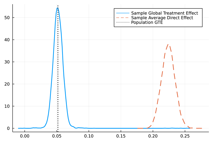
(a) Smoothed empirical distribution of $\tau_{\text{ADE}}$ and $\tau_{GTE}$ over 10,000 samples of $n=2,000$ marketplace.

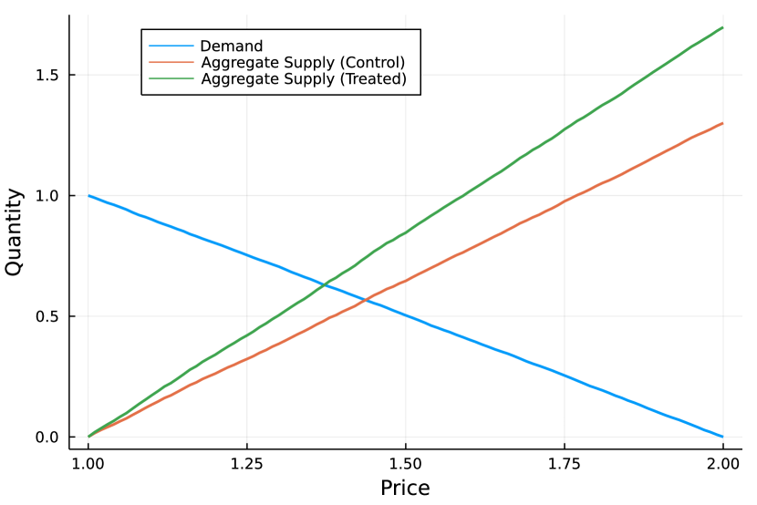
(b) Average excess demand and average excess supply under treatment and control for a single sample of $n=10,000$ marketplace.

Figure 1: Illustration of the gap between $\tau_{\text{ADE}}$ and $\tau_{GTE}$ in the freelance labor model when the intervention has both a direct effect on quantity supplied and an offsetting indirect effect through decreased market-clearing price.

In Figure 1(a), we plot the smoothed distribution of the average direct effect and the global treatment effect, computed over 10,000 samples of a marketplace, where each sample is of 2,000 individuals. An RCT estimates the ADE, which is more than triple the Global Treatment Effect. Figure 1(b) explains why the ADE and GTE are so different in this setting. The figure shows the effect of the treatment on aggregate supply $S(\bm{W},p)=\frac{1}{n}\sum\limits_{i=1}^{n}S_{i}(W_{i},p)$ for a sample of 10,000 individuals. Aggregate demand is unchanged from the treatment. The treatment makes it more likely that already profitable suppliers complete a second job, which shifts the slope of the supply curve. This impacts the market-clearing price for the control market compared to the treated market. Holding market prices fixed, the effect of the treatment is a large positive increase in revenue. However, when the effect on market prices is taken into account, which is represented by a large negative indirect effect, then the global treatment effect is much lower.

In Table 1, we report the results of a Monte Carlo simulation with 10,000 repetitions and a sample size of $n=2,000$ to evaluate the bias, variance, and coverage properties of the estimators and confidence intervals for $\hat{\tau}_{\text{ADE}}$ and $\hat{\tau}_{\text{AIE}}$. The ground truth $\tau^{*}_{\text{ADE}}$ and $\tau^{*}_{\text{AIE}}$ are calculated numerically. The table illustrates that the bias of the average direct effect and indirect effect estimator based on the augmented randomize experiment are low in finite samples. Furthermore, the coverage when $\hat{\sigma}_{D}$ and $\hat{\sigma}_{I}$ are used to construct confidence intervals in finite samples is very close to the asymptotic confidence level of 95%. If only data from an RCT was available, then an estimate for the AIE is not available, while the estimator for the ADE remains a Horvitz-Thompson estimator. The naive confidence interval that assumes no-interference for the direct effect can be computed using data from an RCT. In this simulation, the naive approach gives asymptotically conservative confidence intervals, so has slightly wider confidence intervals, and over-covers compared to the asymptotically exact approach.

	Estimate	Bias	S.D.	Coverage
$\hat{\tau}_{\text{ADE}}$	0.227	0.004	0.06	0.957
$\hat{\tau}_{\text{AIE}}$	-0.173	-0.003	0.05	0.954

Table 1: Monte Carlo Simulation Results for $\hat{\tau}_{\text{ADE}}$ and $\hat{\tau}_{\text{AIE}}$ for a sample of $n=2,000$ and $10,000$ repetitions

5.2 Targeting Cash Transfers

There is a large literature in development economics that randomly allocates cash transfers to households and evaluates the short and long-term impacts on a variety of outcomes, including consumption, savings and investment (Haushofer & Shapiro 2016), health (Haushofer et al. 2020), and criminal behavior (Hidrobo et al. 2016, Blattman et al. 2017).

Depending on the characteristics of the local economies where cash transfers are allocated and the type of outcome evaluated, there may be equilibrium interference that impacts the evaluation of the transfer program. Cunha et al. (2019), for example, find meaningful price impacts for in-kind transfers in an evaluation in Mexico, while Egger et al. (2022) find minimal price impacts for a large scale cash transfer in Kenya. The results in Section 3 indicate that estimating the Global Total Effect of an intervention using data from an RCT requires estimating of elasticities of outcomes, supply, and demand with respect to prices. However, our results in Section 4 indicate that even without price elasticities, we can use data from an RCT to analyze the gain from exploiting heterogeneity in the data when we constrain equilibrium effects under a targeted policy to be equal to that under the RCT.

We examine the publicly available data from the replication package of Gertler et al. (2012), which examined the long-term impacts of PROGRESA, a conditional cash transfer program in Mexico which was rolled out randomly at a community-level, beginning in 1998. The community-level assignment was due to logistical and operational constraints, rather than an attempt to control spillovers, so we expect that given the proximity of treatment and control households, they would have interacted with one another in many markets.

The program included a monthly stipend of 50 pesos per month, and an additional educational stipend, depending on the number of the children in the household, with the total capped at 550 pesos per month. There are 320 treatment communities, which were immediately enrolled in the program, and 186 control communities, which were phased into treatment over time. The data from Gertler et al. (2012) contains a variety of baseline covariates from the 1997 ENCASEH census for households originally classified as poor and eligible for the intervention, as well as measurements from evaluation surveys that were given to all households in treatment and control communities every 6 months, starting in 1998. The evaluation surveys collected a variety of data on household education, consumption, investments, savings, and agricultural income. We follow the original paper in pooling data from October 1998 to November 1999, which was the purely experimental period, before control households began to be enrolled in the program. We are interested in using a subset of the data to answer a specific question, which is how a policymaker could target a PROGRESA-like subsidy to households to maximize agricultural income, when land usage under the targeted policy is constrained to be equal to that of the RCT. We compute the structure of the targeting rule, and estimate how much the optimal targeted policy raises outcomes compared to the uniform policy.

Before describing our results, we first explain a few caveats that should be kept in mind. First, depending on how quickly prices adjust and the geographic proximity of treated and control households, the community-level assignment could result in different equilibrium conditions for treated and control households. For the purposes of illustrating our method, we assume that treated and control individuals are responding to similar market prices in the experimental period, so that the conditional direct effects we measure do not include an equilibrium effect. Second, a general cash subsidy likely results in equilibrium effects of varying strength that occur through an enormous variety of channels, including the labor market, commodities markets, and even financial markets. For this exercise, we assume that the farm subsidy has an equilibrium effect on outcomes through a single good only, which is the usage of land. Last, it is possible that the usage of land is very slack, so that if the treatment increases usage of land, there is no effect on the actual market demand for land. We assume that the net usage of land does proxy for the net market demand for land in our sample, so that our constraint on land usage corresponds to an equilibrium stability condition.

In Figure 2, we illustrate the optimal rule estimated using a sample of $n=33,182$ households from Waves 2-4 of the survey. There are 20 covariates in $X_{i}$, which are all pre-treatment household demographic characteristics from 1997, such as age and gender of the head of household, the existing landholdings and animal ownership of the household, and whether or not the house had electricity. The outcome $Y_{i}$ is agricultural income per individual in the household, including crop sales, sales from animal products, and home consumption. Ignoring equilibrium effects, a good targeting rule allocates treatment to those individuals who are estimated to have a positive CADE. This rule, however, results in a larger impact on demand for land compared to the RCT, since on average, those who increase their agricultural income using the subsidy also increase their usage of land. However, there is some heterogeneity in the usage of land. The optimal rule that respects the equilibrium constraint allocates treatment to those with $\hat{\tau}^{Y}_{\text{CADE}}(X_{i})>c\hat{\tau}^{Z}_{\text{CADE}}(X_{i})$. We can see that for the most part, it is those with a positive CADE that are treated. However, those with a large $\frac{-\hat{\tau}^{Z}_{\text{CADE}}(X_{i})}{\hat{\tau}^{Y}_{\text{CADE}}(X_{i})}$ have their treatment status flipped from the naive rule that ignores the equilibrium constraints. Those, for example, who use a lot of additional land but have a small impact on agricultural income, are dropped from the equilibrium-stable targeting rule.

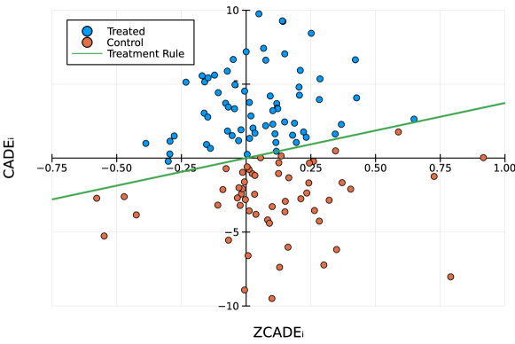
Figure 2: A scatter-plot of an estimate of $\tau_{\text{CADE}}(X_{i})$ and $\tau^{Z}_{\text{CADE}}(X_{i})$ for a sample of 125 households, estimated using the causal forest of Athey et al. (2019). Overlaid is the optimal equilibrium-stable targeting rule, computed by solving a plug-in version of the linear program in Theorem 9 on random training split of $n=10,822$, which takes the form of the rule in Proposition 11.

	Gain	Equilibrium-Stability	$\bm{c}$
Estimate	2.27	-0.006	0.92
Standard Error	(0.44)	(0.021)	(1.12)

Table 2: Estimated out-of-sample performance of equilibrium-stable targeting rule. Standard errors computed using the bootstrap.

We then evaluate the gain in the targeted rule compared to the uniform rule using the data-splitting approach described at the end of Section 4.2. The results are reported in Table 2. We find that the lift is 2.27 and significantly different from zero at a 5% level. In this example, there is modest heterogeneity in outcomes and demand for land. When this is exploited via the optimal equilibrium-stable targeting rule, the point estimate for the gain over the uniform rule is positive and large. The equilibrium stability metric is -0.006 with a standard error of 0.44, so on average the treatment rule estimated on the training set is disturbing the equilibrium on the test set by a very small amount, compared to the uniform rule.

6 Discussion

Analyzing the performance of randomized control trials in settings with equilibrium effects is needed given the rapid growth of experimentation both in practice and in research studies. The Neyman-Rubin framework that relies on SUTVA rules out interaction effects that can have an important impact on decision-relevant treatment effects. A parametric structural model may capture a variety of complex equilibrium effects, but is not robust to misspecification, which can be problematic when individuals behave in complex and heterogeneous ways. A model of treatment effects under general patterns of interference is intractable without clustering or other assumptions.

This paper shows that it is fruitful to marry ex-ante knowledge about the structure of an economic environment with a non-parametric stochastic model of treatment effects under interference. This leads to a characterization of asymptotic properties of treatment effects and estimators of those treatment effects based on new and existing experimental designs that are robust to a wide range of modeling choices. Results on estimation, inference, and optimal targeting in complex environments with some economic structure imposed can then be easily contrasted with the large body of work that studies casual inference under SUTVA.

There are a variety of avenues for future work possible. One limitation of our approach is that we analyze the large sample limit of the market place where the number of suppliers and the number of buyers grow large; an analysis of experiments in settings where firms have significant market power would likely require different techniques. In general, extending our results to a broader class of equilibrium mechanisms would be of considerable interest.

Appendix A Main Results

A.1 Notation

We first include a brief comment on the asymptotic notations used in the proofs. We use asymptotic notations such as $O(\cdot)$ and $o(\cdot)$ in the conventional sense. In particular, we use $\bm{A}_{n}=O_{p}(\alpha_{n})$ if for every $\epsilon$, there exists an $c<\infty$ such that $\lim\limits_{n\rightarrow\infty}\mathbb{P}\{\|\bm{A}_{n}\|>\alpha_{n}c\}<\epsilon$. Similarly, we use $\bm{A}_{n}=o_{p}(\alpha_{n})$ if, for all $c>0$, $\lim\limits_{n\rightarrow\infty}\mathbb{P}\{\|\bm{A}_{n}\|>\alpha_{n}c\}=0$.

A.2 Uniqueness of Mean-Field Market Price (Proposition 1)

The proof of uniqueness in this section makes use of the Banach fixed point theorem.

Lemma 12.

Banach Fixed Point Theorem: Consider a set $D\subset\mathbb{R}^{J}$ and a function $g:D\rightarrow R^{J}$. If

1. $D$ is closed,

2. $x\in D$ implies that $g(\bm{x})\in D$, and

3. $g$ is a contraction on D, meaning there exists a $0\leq q<1$ such that for all $\bm{x},\bm{y}\in D$, we have that

   $$\|g(\bm{x})-g(\bm{y})\|\leq q\|\bm{x}-\bm{y}\|,$$

then, there exists a unique $\bm{x}^{*}\in D$ with $g(\bm{x}^{*})=\bm{x}^{*}$.

Lemma 13.

Contraction Property Assume that the set $D\subset R^{J}$ is convex and the function $g$ has continuous partial derivatives. If $\|\nabla g(x)\|<1$, then the mapping $g$ is a contraction in $D$.

Now, we can prove Proposition 1. We first prove that the mean-field equilibrium price exists and is unique. Let $\bm{f}(\bm{p})=\mathbb{E}[\bm{Z}_{i}(W_{i},\bm{p})]+\bm{p}$ be a function from $\mathbb{R}^{J}$ to $\mathbb{R}^{J}$. Then Lemma 13 indicates that $\bm{f}(\bm{p})$ is a contraction mapping, since we assume that $\|\nabla\bm{f}(p)\|<1$. By Lemma 12, then there is a unique fixed point

$$\bm{f}(\bm{p}^{*})=\bm{p}^{*},$$

which occurs when $\mathbb{E}[\bm{Z}_{i}(W_{i},\bm{p}^{*})]=0$. This means that the set $\{\bm{p}:\mathbb{E}[\bm{Z}_{i}(W_{i},\bm{p})]=0\}$ has a unique element, which means that the mean-field equilibrium price $\bm{p}^{*}_{\pi}$ is unique.

A.3 Convergence of Market Price

The below lemma is not used directly in the main text, but various steps in this proof are used elsewhere in the proof of the main results.

Lemma 14.

Under Assumptions 2–4, the finite sample equilibrium price converges in probability to the mean-field price $\bm{p}^{*}_{\pi}$:

$$\bm{P}_{n}\rightarrow_{p}\bm{p}^{*}_{\pi},\quad\mbox{ as $n\to\infty$.}$$

Note that in this section, we prove this for a more general, perturbed system, where individuals receive market price ${\bm{P}}_{n}(\bm{W},\bm{U})$, and prices are perturbed by $\bm{U}_{i}$. The results hold for any $\bm{U}_{i}\rightarrow 0$. So, they also hold for $\bm{U}_{i}=0$, which proves Lemma 14 for price $\bm{P}_{n}(\bm{W})$.

We use Theorem 5.9 of van der Vaart (1998), which requires verifying two conditions.

Lemma 15.

Theorem 5.9 of van der Vaart (1998):

Let $\bm{M}_{n}$ be random vector-valued functions and let $\bm{\mu}$ be a fixed vector-valued function of $\phi$ such that for every $\epsilon>0$:

$$\begin{split}&\sup_{\bm{\phi}\in\Phi}\|\bm{M}_{n}(\bm{\phi})-\bm{\mu}(\bm{\phi})\|\rightarrow_{p}0,\\ &\inf_{\bm{\phi}:d(\bm{\phi},\bm{\phi}_{0})\geq\epsilon}\|\bm{\mu}(\bm{\phi})\|>0=\|\bm{\mu}(\bm{\phi}_{0})\|.\end{split}$$

Then any sequence of estimators $\hat{\bm{\phi}}_{n}$ such that $\bm{M}_{n}(\hat{\bm{\phi}}_{n})=o_{p}(1)$ converges in probability to $\bm{\phi}_{0}$.

Let $\bm{Z}_{n}(\bm{p})=\frac{1}{n}\bm{Z}_{i}(W_{i},\bm{p}+\bm{U}_{i})$ and $\bm{z}(\bm{p})=\mathbb{E}[Z_{i}(W_{i},\bm{p})]$. We first show the uniform convergence of the estimating equation for the finite sample price $\bm{Z_{n}}(\bm{p})$ to the estimating equation for the mean-field price $\mathbb{E}[\bm{Z}_{i}(W_{i},\bm{p})]$.

Lemma 16.

Under Assumptions 2–4, the finite sample average excess demand converges uniformly to the expected excess demand,

$$\sup_{\bm{p}\in\mathcal{S}}\|\bm{Z_{n}}(\bm{p})-\bm{z}(\bm{p})\|\rightarrow_{p}0.$$

Proof.

We have that

$$\begin{split}\sup_{\bm{p}\in\mathcal{S}}\|\bm{Z_{n}}(\bm{p})-\bm{z}(\bm{p})]\|&\leq\sup_{\bm{p}\in\mathcal{S}}\|\bm{Z_{n}}(\bm{p})-\mathbb{E}[\bm{Z}_{i}(W_{i},\bm{p}+\bm{U}_{i})]\|+\sup_{\bm{p}\in\mathcal{S}}\|\mathbb{E}[\bm{Z}_{i}(W_{i},\bm{p}+\bm{U}_{i})]-\mathbb{E}[\bm{Z}_{i}(W_{i},\bm{p})\|\\ &\rightarrow_{p}0\end{split}$$

The uniform convergence

$$\sup_{\bm{p}\in\mathcal{S}}\|\bm{Z_{n}}(\bm{p})-\mathbb{E}[\bm{Z}_{i}(W_{i},\bm{p}+\bm{U}_{i})]\|\rightarrow_{p}0$$

follows directly from Lemma 2.4 of Newey & McFadden (1994), since we have from Assumption 3 that $\bm{Z}_{i}(w,\bm{p})$ is weakly continuous and bounded and that $\mathcal{S}$ is compact.

Since $\mathbb{E}[\bm{Z}_{i}(W_{i},\bm{p}+\bm{U}_{i})]$ is differentiable with a bounded first derivative then it is uniformly continuous, and then $\sup_{\bm{p}\in\mathcal{S}}\|\mathbb{E}[\bm{Z}_{i}(W_{i},\bm{p}+\bm{U}_{i})]-\mathbb{E}[\bm{Z}_{i}(W_{i},\bm{p})\|\rightarrow_{p}0$ follows from the uniform continuous mapping theorem, since $\bm{U}_{i}\rightarrow_{p}0$.

∎

The following lemma (the proof is Problem 5.27 of van der Vaart (1998)) is useful for verifying the second condition.

Lemma 17.

Strict Zero. If a function $\bm{\mu}:\Phi\rightarrow\mathbb{R}^{k}$ is continuous and has a unique zero at $\phi_{0}$, then if $\Phi$ is compact, we have that for every $\epsilon>0$:

$$\inf_{\phi:d(\phi,\phi_{0})\geq\epsilon}\|\bm{\mu}(\phi)\|>0=\|\bm{\mu}(\phi_{0})\|.$$

We show that the mean-field price is a strict zero in the following lemma:

Lemma 18.

The mean-field price is a strict zero. Under Assumptions 2–4, for all $\epsilon>0$,

$$\inf_{\bm{p}:d(\bm{p},\bm{p}^{*}_{\pi})\geq\epsilon}\|\mathbb{E}[\bm{Z}_{i}(W_{i},\bm{p})]\|>0=\|\mathbb{E}[\bm{Z}_{i}(W_{i},\bm{p}^{*}_{\pi})]\|.$$

Proof.

The proof follows immediately from Lemma 17 since $\mathcal{S}$ is compact, $\bm{z}(\bm{p})$ is continuous in $\bm{p}$, and $\bm{p}^{*}_{\pi}$ is unique. ∎

Since we have from the version of Assumption 3.5 in Proposition 5, that that $\bm{Z}_{n}(\tilde{\bm{P}})=o_{p}(n^{-0.5})$, where $\bm{Z}_{n}(p)=\frac{1}{n}\sum\limits\bm{Z}_{i}(W_{i},\bm{p}+\bm{U}_{i})$, then we have met all the conditions of Lemma 15 and we have proved that

$$\tilde{\bm{P}}\rightarrow_{p}\bm{p}^{*}_{\pi}.$$

A.4 Rate of Market Price Convergence (Theorem 2 and Proposition 5)

We first prove a more general version of Theorem 2 for the perturbed system with market prices ${\bm{P}}_{n}(\bm{W},\bm{U})$.

Theorem 19.

Under Assumptions 2-4, the finite sample equilibrium price in the price experiment converges in distribution to the mean-field price and is asymptotically normal:

$$\sqrt{n}(\tilde{\bm{P}}_{n}-\bm{p}^{*}_{\pi})\rightarrow_{d}N(0,\bm{\xi}_{z}^{-1}\mathbb{E}[\bm{Z}_{i}(W_{i},\bm{p}^{*}_{\pi})\bm{Z}_{i}(W_{i},\bm{p}^{*}_{\pi})^{\top}]\bm{\xi}_{z}^{-1}).$$

Proof.

The following result from theory of Z-estimators is used in this proof. We replace the Lipschitz condition from the original Theorem 5.21 with the Donsker condition discussed in Lemma 19.24 of van der Vaart (1998).

Lemma 20.

Modified Theorem 5.21 of van der Vaart (1998) : For each $\bm{\phi}$ in an open subset of Euclidean space, let $\bm{x}\mapsto\bm{m}_{\phi}(\bm{x})$ be a measurable vector-valued function, such that the class $\{\bm{m}_{\phi}:||\bm{\phi}-\bm{\phi}_{0}||<\delta\}$ is Donsker for some $\delta>0$ and $\mathbb{E}[(\bm{m}_{\hat{\bm{\phi}}_{n}}(\bm{X}_{i})-\bm{m}_{\bm{\phi}_{0}}(\bm{X}_{i}))^{2}]\rightarrow_{p}0$. Assume that $\mathbb{E}[\|\bm{m}_{\phi_{0}}(\bm{X}_{i})\|^{2}]<\infty$ and that the map $\bm{\phi}\mapsto\mathbb{E}[\bm{m}_{\phi}(\bm{X}_{i})]$ is differentiable at a zero $\bm{\phi}_{0}$, with nonsingular derivative matrix $\bm{V}_{\phi_{0}}$. If $\frac{1}{n}\sum\limits_{i=1}^{n}\bm{m}_{\hat{\bm{\phi}}_{n}}(\bm{X}_{i})=o_{p}(n^{-1/2})$ and $\hat{\bm{\phi}}_{n}\rightarrow_{p}\bm{\phi}_{0}$, then:

$$\sqrt{n}(\hat{\bm{\phi}}_{n}-\bm{\phi}_{0})=-\bm{V}_{\bm{\phi}_{0}}^{-1}\frac{1}{\sqrt{n}}\sum\limits_{i=1}^{n}m_{\bm{\phi}_{0}}(\bm{X}_{i})+o_{p}(1).$$

We verify each of the conditions of Lemma 20.

• We can show the required quadratic mean convergence using Lemma 30, where $F_{i}(\bm{p})=\bm{Z}_{i}(W_{i},\bm{p}+\bm{U}_{i})$, where the required assumptions are in Assumption 3 - 4.

• By Assumption 3, the class of functions $\bm{Z}_{i}(w,\bm{p})$ indexed by $\bm{p}$ is Donsker.

• Since $\bm{Z}_{i}(w,\bm{p})$ is bounded, then $\mathbb{E}[\|\bm{Z}_{i}(W_{i},\bm{p}^{*}_{\pi}+\bm{U}_{i})\|^{2}]<\infty$.

• By Lemma 14, we have that $\tilde{\bm{P}}_{n}\rightarrow_{p}\bm{p}^{*}_{\pi}$.

• By the differentiability of $\bm{z}(w,\bm{p})$, $\nabla_{p}\mathbb{E}[\bm{Z}_{i}(W_{i},\bm{p}^{*}_{\pi}+\bm{U}_{i})]$ exists. Furthermore, by the continuous mapping theorem, since $\bm{U}_{i}\rightarrow_{p}0$, $\nabla_{p}\mathbb{E}[\bm{Z}_{i}(W_{i},\bm{p}^{*}_{\pi}+\bm{U}_{i})]\rightarrow_{p}\bm{\xi}_{z}$ which is non-singular by Assumption 4.

Then, we can apply Theorem 5.21 of van der Vaart (1998):

$$\sqrt{n}(\tilde{\bm{P}}-\bm{p}^{*}_{\pi}) =-[\bm{\xi}_{z}]^{-1}\frac{1}{\sqrt{n}}\sum\limits_{i=1}^{n}\bm{Z}_{i}(W_{i},\bm{p}^{*}_{\pi}+\bm{U}_{i})+o_{p}(1)$$ (9)

$$=-[\bm{\xi}_{z}]^{-1}\frac{1}{\sqrt{n}}\sum\limits_{i=1}^{n}\Big{[}\bm{Z}_{i}(W_{i},\bm{p}^{*}_{\pi}+\bm{U}_{i})-\mathbb{E}[\bm{Z}_{i}(W_{i},\bm{p}^{*}_{\pi}+\bm{U}_{i})]\Big{]}$$

$$+\sqrt{n}\bm{\xi}_{z}^{-1}(\mathbb{E}[\bm{Z}_{i}(W_{i},\bm{p}^{*}_{\pi})]-\mathbb{E}[\bm{Z}_{i}(W_{i},\bm{p}^{*}_{\pi}+\bm{U}_{i})])+o_{p}(1)$$

$$=-[\bm{\xi}_{z}]^{-1}\frac{1}{\sqrt{n}}\sum\limits_{i=1}^{n}\Big{[}\bm{Z}_{i}(W_{i},\bm{p}^{*}_{\pi}+\bm{U}_{i})-\mathbb{E}[\bm{Z}_{i}(W_{i},\bm{p}^{*}_{\pi}+\bm{U}_{i})]\Big{]}+o_{p}(1)$$ (10)

Where the last equality comes from Lemma 29, since $\mathbb{E}[\bm{z}(w,\bm{p}+\bm{U}_{i})]$ is continuous in $\bm{p}$. We can now apply the CLT to the sum in (10) after scaling by the variance.Let $\bm{1}_{J}$ be the $J\times J$ identity matrix:

$$\left[\frac{1}{\sqrt{n}}\sum\limits_{i=1}^{n}\bm{Z}_{i}(W_{i},\bm{p}^{*}_{\pi}+\bm{U}_{i})-\mathbb{E}[\bm{Z}_{i}(W_{i},\bm{p}^{*}_{\pi}+\bm{U}_{i})]\right]\left[\mbox{Var}(\bm{Z}_{i}(W_{i},\bm{p}^{*}_{\pi}+\bm{U}_{i}))\right]^{-1}\rightarrow_{d}N(0,\bm{1}_{J})$$

Assumption 4 indicates that each element of the variance of $\bm{Z}_{i}(w,\bm{p})$ is continuous in $\bm{p}$. We can use the CMT to show that $\mbox{Var}(\bm{Z}_{i}(W_{i},\bm{p}^{*}_{\pi}+\bm{U}_{i}))=\mathbb{E}[\bm{Z}_{i}(W_{i},\bm{p}^{*}_{\pi})^{2}]+o_{p}(1)$ since $\bm{U}_{i}\rightarrow_{p}0$. We have now shown that

$$\sqrt{n}(\tilde{\bm{P}}-\bm{p}^{*}_{\pi})\rightarrow_{d}N(0,\bm{\xi}_{z}^{-1}\mathbb{E}[\bm{Z}_{i}(W_{i},\bm{p}^{*}_{\pi})\bm{Z}_{i}(W_{i},\bm{p}^{*}_{\pi})^{\top}]\bm{\xi}_{z}^{-1}).$$

∎

Proof of Theorem 2 and Proposition 5

Theorem 2 follows directly from Theorem 19. The results hold for any $\bm{U}_{i}=cn^{-\alpha}$, with $\alpha>\frac{1}{4}$ and finite $c$. Thus, the conclusions hold for $\bm{P}_{n}(\bm{W})={\bm{P}}_{n}(\bm{W},\bm{0})$.

For the Proposition, the expansion in Equation 9 indicates that

$$\sqrt{n}(\bm{P}_{n}-\tilde{\bm{P}}_{n})=[\bm{\xi}_{z}]^{-1}\frac{1}{\sqrt{n}}\sum\limits_{i=1}^{n}[\bm{Z}_{i}(W_{i},\bm{p}^{*}_{\pi}+\bm{U}_{i})-\bm{Z}_{i}(W_{i},\bm{p}^{*}_{\pi})]+o_{p}(1).$$

Since we have that $\bm{p}^{*}_{\pi}+\bm{U}_{i}\rightarrow_{p}\bm{p}^{*}_{\pi}$, and $\bm{Z}_{i}(W_{i},\bm{p})$ is bounded and continuous with probability $1$ in $\bm{p}$, then we have the quadratic mean convergence $\mathbb{E}[(Z_{i}(W_{i},\bm{p}^{*}_{\pi}+\bm{U}_{i})-\bm{Z}_{i}(W_{i},\bm{p}^{*}_{\pi}))^{2}]\rightarrow 0$ (see Lemma 30 for a more detailed argument). Then, from the Donsker assumption of Assumption 3, we can use Lemma 19.24 of van der Vaart (1998) to show that the expansion above is equivalent to:

$$\sqrt{n}(\bm{P}_{n}-\tilde{\bm{P}}_{n}) =[\bm{\xi}_{z}]^{-1}\sqrt{n}\mathbb{E}[\bm{Z}_{i}(W_{i},\bm{p}^{*}_{\pi}+\bm{U}_{i})]-\mathbb{E}[\bm{Z}_{i}(W_{i},\bm{p}^{*}_{\pi})]+o_{p}(1)$$

$$=o_{p}(1)$$

where the second equality is from Lemma 29 since $\alpha>\frac{1}{4}$. The proof of the second part of Proposition 5 follows from Lemma 26, the proof of which is later in the Appendix.

A.5 Proof of Mean-Field Causal Effects (Theorem 3)

Convergence of ADE

Proof.

As implied by the technical appendix of Sävje et al. (2021) and in Hu et al. (2022), we have that the Horvitz-Thompson estimator is unbiased for the direct effect.

$$\hat{\tau}_{\text{ADE}}=\frac{1}{n}\sum\limits_{i=1}^{n}\frac{W_{i}Y_{i}(W_{i},\bm{P}_{n}(\bm{W}))}{\pi_{i}}-\frac{(1-W_{i})Y_{i}(W_{i},\bm{P}_{n}(\bm{W}))}{1-\pi_{i}}.$$

Taking expectation, we have that

$$\mathbb{E}_{\pi}[\hat{\tau}_{\text{ADE}}]=\frac{1}{n}\sum\limits_{i=1}^{n}\mathbb{E}_{\pi}[Y_{i}(W_{i},\bm{P}_{n}(\bm{W}))|W_{i}=1]-\mathbb{E}_{\pi}[Y_{i}(W_{i},\bm{P}_{n}(\bm{W}))|W_{i}=0]=\tau_{\text{ADE}}.$$

Subtracting $\tau^{*}_{ADE}$ from both sides of $\tau_{\text{ADE}}=\mathbb{E}_{\pi}[\hat{\tau}_{\text{ADE}}]$,

$$\tau_{\text{ADE}}-\tau^{*}_{ADE}=\mathbb{E}_{\pi}[\hat{\tau}_{\text{ADE}}-\tau^{*}_{ADE}].$$

Next, we show that $\hat{\tau}_{\text{ADE}}\rightarrow_{p}\tau^{*}_{ADE}$. By the expansion in Lemma 30, and the convergence of $\bm{P}_{n}(\bm{W})$ to $\bm{p}^{*}_{\pi}$ in probability, we have that

$$\hat{\tau}_{\text{ADE}} =\frac{1}{n}\sum\limits_{i=1}^{n}\frac{W_{i}Y_{i}(W_{i},\bm{p}^{*}_{\pi})}{\pi_{i}}-\frac{(1-W_{i})Y_{i}(W_{i},\bm{p}^{*}_{\pi})}{1-\pi_{i}}+o_{p}(1)$$

$$=y(1,\bm{p}^{*}_{\pi})-y(0,\bm{p}^{*}_{\pi}),$$

where the second line is from the LLN. $\hat{\tau}_{\text{ADE}}$ is uniformly bounded, since it is the average of uniformly bounded functions and $\pi_{i}$ is bounded away from 0 and 1. So, we have that $\hat{\tau}_{\text{ADE}}=\tau^{*}_{ADE}+o_{p}(1)$ implies that $\mathbb{E}_{\pi}[\hat{\tau}_{\text{ADE}}-\hat{\tau}^{*}_{ADE}]=o_{p}(1)$.

Since $\hat{\tau}_{\text{ADE}}$ is an average of uniformly bounded functions, it is also uniformly bounded. So, we have , where $B$ is finite, that for any $\epsilon>0$, $\mathbb{E}_{\pi}[\hat{\tau}_{\text{ADE}}-\tau^{*}_{ADE}]\leq BPr_{\pi}(\hat{\tau}_{\text{ADE}}-\tau_{\text{ADE}}^{*}>\epsilon/2)+\epsilon/2$. This implies $Pr(\mathbb{E}_{\pi}[\hat{\tau}_{\text{ADE}}-\tau^{*}_{ADE}]>\epsilon)\leq Pr(\hat{\tau}_{\text{ADE}}-\tau^{*}_{ADE}>\epsilon/2)\rightarrow 0$. We have now shown that $\mathbb{E}_{\pi}[\hat{\tau}_{\text{ADE}}-\tau^{*}_{ADE}]=o_{p}(1)$, which finishes the proof.

∎

Convergence of AIE

Proof.

The first step is to prove a probability limit for $\tau_{\text{INF}}$, which is

$$\tau_{\text{INF}}=\sum\limits_{k=1}^{n}\frac{\partial}{\partial\pi_{k}}\frac{1}{n}\sum\limits_{i=1}^{n}\mathbb{E}_{\pi}[Y_{i}(W_{i},\bm{P}_{n})].$$

Recall that $W_{i}\sim\mbox{Bernoulli}(\pi_{i})$, we can expand the expectation with respect to $\bm{W}$:

$$\tau_{\text{INF}}=\sum\limits_{k=1}^{n}\frac{\partial}{\partial\pi_{k}}\sum\limits_{\bm{w}^{j}}\frac{1}{n}\sum\limits_{i=1}^{n}f(\bm{w}^{j})Y_{i}(w^{j}_{i},\bm{P}_{n}(\bm{w}^{j})),$$

where $f(\bm{w}^{k})=\prod_{k=1}^{n}\pi_{k}^{w^{j}_{k}}(1-\pi_{k})^{1-w^{j}_{k}}$. We can take the derivative and manipulate to get

$$\frac{\partial}{\partial\pi_{k}}f(\bm{w}^{j})=\frac{w^{j}_{k}-\pi_{k}}{\pi_{k}(1-\pi_{k})}f(\bm{w}^{j}).$$

This allows us to write

$$\begin{split}\tau_{\text{INF}}&=\sum\limits_{k=1}^{n}\frac{\partial}{\partial\pi_{k}}\sum\limits_{\bm{w}^{j}}\frac{w^{j}_{k}-\pi_{k}}{\pi_{k}(1-\pi_{k})}f(\bm{w}^{j})\frac{1}{n}\sum\limits_{i=1}^{n}Y_{i}(w^{k}_{i},\bm{P}_{n}(\bm{w}^{k}))\\ &=\mathbb{E}_{\pi}\left[\sum\limits_{k=1}^{n}\frac{W_{k}-\pi_{k}}{\pi_{k}(1-\pi_{k})}\frac{1}{n}\sum\limits_{i=1}^{n}Y_{i}(W_{i},\bm{P}_{n}(\bm{W}))\right]\end{split}$$ (11)

We will use the following Lemma in the next few steps, which is proved in Appendix B.2.

Lemma 21.

Under the Assumptions of Theorem 3, for each of the below remainder terms $m\in\{1,2,3\}$, $\mathbb{E}_{\pi}\left[\sum\limits_{k=1}^{n}\frac{W_{k}-\pi_{k}}{\pi_{k}(1-\pi_{k})}R_{mn}\right]\rightarrow_{p}0$

$$R_{1n}=\frac{1}{n}\sum\limits_{i=1}^{n}Y_{i}(W_{i},\bm{P}_{n})-\mathbb{E}[Y_{i}(W_{i},\bm{P}_{n})]-(Y_{i}(W_{i},\bm{p}^{*}_{\pi})-\mathbb{E}[Y_{i}(W_{i},\bm{p}^{*}_{\pi})])$$ (12)

$$R_{2n}\leq||\bm{P}_{n}-\bm{p}^{*}_{\pi}||^{2}D$$ (13)

$$R_{3n}=\bm{\xi}_{y}^{\top}\left[(\bm{P}_{n}-\bm{p}^{*}_{\pi})+\bm{\xi}_{z}^{-1}\frac{1}{n}\sum\limits_{i=1}^{n}\bm{Z}_{i}(W_{i},\bm{p}^{*}_{\pi})\right],$$ (14)

where $D$ is a finite constant.

We now use the expansion from Lemma 30, where $F_{i}(\bm{p})=Y_{i}(W_{i},\bm{p})$. The expansion is valid since $\bm{P}_{n}(\bm{W})=\bm{p}^{*}_{\pi}+O_{p}(n^{-0.5})$ (see Theorem 2) and Assumption 3 - 4 provides the necessary continuity and differentiability properties. The expansion is

$$\frac{1}{n}\sum\limits_{i=1}^{n}Y_{i}(W,\bm{P}_{n}(\bm{W})=\frac{1}{n}\sum\limits_{i=1}^{n}Y_{i}(W_{i},\bm{p}^{*}_{\pi})+(\bm{P}_{n}(\bm{W})-\bm{p}^{*}_{\pi})^{\top}\bm{\xi}_{y}+R_{1n}+R_{2n},$$

where $R_{1n}$ and $R_{2n}$ are each $o_{p}(n^{-0.5})$ and are defined in Lemma 21. Plugging this expansion into (11),

$$\tau_{\text{INF}} =\mathbb{E}_{\pi}\left[\sum\limits_{k=1}^{n}\frac{W_{k}-\pi_{k}}{\pi_{k}(1-\pi_{k})}\left[\frac{1}{n}\sum\limits_{i=1}^{n}Y_{i}(W_{i},\bm{p}^{*})+(\bm{P}_{n}(\bm{W})-\bm{p}^{*}_{\pi})^{\top}\bm{\xi}_{y}\right]\right]$$ (15)

$$\qquad+\mathbb{E}_{\pi}\left[\sum\limits_{k=1}^{n}\frac{W_{k}-\pi_{k}}{\pi_{k}(1-\pi_{k})}(R_{1n}+R_{2n})\right]$$

$$=\mathbb{E}_{\pi}\left[\sum\limits_{k=1}^{n}\frac{W_{k}-\pi_{k}}{\pi_{k}(1-\pi_{k})}\left[\frac{1}{n}\sum\limits_{i=1}^{n}Y_{i}(W_{i},\bm{p}^{*})+(\bm{P}_{n}(\bm{W})-\bm{p}^{*}_{\pi})^{\top}\bm{\xi}_{y}\right]\right]+o_{p}(1).$$ (16)

We deal with the remainder term using Lemma 21. We can now work with the first part of the expectation directly. Examine $\sum\limits_{k=1}^{N}\frac{W_{k}-\pi_{k}}{\pi_{k}(1-\pi_{k})}$ and notice that $Y_{i}(W_{i},\bm{p}^{*}_{\pi})$ is independent of all elements of that sum except for $W_{i}-\pi_{i}$.

$$\mathbb{E}_{\pi}\left[\sum\limits_{k=1}^{N}\frac{W_{k}-\pi_{k}}{\pi_{k}(1-\pi_{k})}\frac{1}{n}\sum\limits_{i=1}^{n}Y_{i}(W_{i},\bm{p}^{*})\right] =\frac{1}{n}\sum\limits_{i=1}^{n}\frac{\mathbb{E}_{\pi}[(W_{i}-\pi_{i})Y_{i}(W_{i},\bm{p}^{*})]}{\pi_{i}(1-\pi_{i})}$$

$$=\frac{1}{n}\sum\limits_{i=1}^{n}Y_{i}(1,\bm{p}^{*})-Y_{i}(0,\bm{p}^{*})$$ (17)

By a similar argument, we work with the second part of the expectation. We can substitute the expansion from Lemma 20 which indicates

$$(\bm{P}_{n}-\bm{p}^{*}_{\pi})=-\bm{\xi}_{z}^{-1}\frac{1}{n}\sum\limits_{i=1}^{n}\bm{Z}_{i}(W_{i},\bm{p}^{*}_{\pi})+R_{3n},$$

where $R_{3n}=o_{p}(n^{-0.5})$. Again, we have that $\bm{Z}_{i}(W_{i},\bm{p}^{*}_{\pi})$ is independent of all elements of the sum $\sum\limits_{k=1}^{N}\frac{W_{k}-\pi_{k}}{\pi_{k}(1-\pi_{k})}$ except for $W_{i}-\pi_{i}$.

$$\mathbb{E}\left[\sum\limits_{k=1}^{N}\frac{W_{k}-\pi_{k}}{\pi_{k}(1-\pi_{k})}(\bm{P}_{n}(\bm{W})-\bm{p}^{*}_{\pi})\bm{\xi}_{y}\right] =\mathbb{E}\left[\sum\limits_{k=1}^{N}\frac{W_{k}-\pi_{k}}{\pi_{k}(1-\pi_{k})}(\bm{\xi}_{z})^{-1}\frac{1}{n}\sum\limits_{i=1}^{n}\bm{Z}_{i}(W_{i},\bm{p}^{*})\right]$$ (18)

$$\qquad+\mathbb{E}_{\pi}\left[\sum\limits_{k=1}^{N}\frac{W_{k}-\pi_{k}}{\pi_{k}(1-\pi_{k})}(R_{3n})\right]$$

$$=\frac{1}{n}\bm{\xi}_{z}^{-1}\sum\limits_{i=1}^{n}\frac{\mathbb{E}[(W_{i}-\pi_{i})\bm{Z}_{i}(W_{i},\bm{p}^{*})]}{\pi_{i}(1-\pi_{i})}+o_{p}(1)$$

$$=\frac{1}{n}\bm{\xi}_{z}^{-1}\sum\limits_{i=1}^{n}\bm{Z}_{i}(1,\bm{p}^{*})-\bm{Z}_{i}(0,\bm{p}^{*})+o_{p}(1),$$ (19)

where the remainder term converges in probability to zero by Lemma 21. Substituting (17) and (19) into (16), we have now shown that.

$$\tau_{\text{INF}}=\frac{1}{n}\sum\limits_{i=1}^{n}Y_{i}(1,\bm{p}^{*})-Y_{i}(0,\bm{p}^{*})-\bm{\xi}_{y}^{\top}[\bm{\xi}_{z}]^{-1}\frac{1}{n}\sum\limits_{i=1}^{n}(\bm{Z}_{i}(1,\bm{p}^{*})-\bm{Z}_{i}(0,\bm{p}^{*}))+o_{p}(1)$$

We can now apply the LLN to show that

$$\tau_{\text{INF}} =y(1,\bm{p}^{*}_{\pi})-y(0,\bm{p}^{*}_{\pi})-\bm{\xi}_{y}[\bm{\xi}_{z}]^{-1}[\bm{z}(1,\bm{p}^{*}_{\pi})-\bm{z}(0,\bm{p}^{*}_{\pi})]+o_{p}(1)=\tau^{*}_{\text{INF}}$$

We now use this probability limit to derive the limit of $\tau_{\text{AIE}}$. Theorem 1 of Hu et al. (2022) indicates that

$$\tau_{\text{INF}}=\tau_{\text{ADE}}+\tau_{\text{AIE}}.$$

Since we have already proved in the previous section that $\tau_{\text{ADE}}\rightarrow_{p}\tau^{*}_{\text{ADE}}$, then $\tau_{\text{AIE}}\rightarrow_{p}\tau^{*}_{\text{AIE}}$, where

$$\tau^{*}_{\text{AIE}}=\tau^{*}_{\text{INF}}-\tau^{*}_{\text{ADE}}.$$

We have now proved that

$$\tau^{*}_{\text{AIE}}=-\bm{\xi}_{y}[\bm{\xi}_{z}]^{-1}[\bm{z}(1,\bm{p}^{*}_{\pi})-\bm{z}(0,\bm{p}^{*}_{\pi})].$$

∎

A.6 Proof of Estimator Consistency

This theorem does not appear in the main text but is useful in the proof of other results.

Theorem 22.

Under the assumptions of Theorem 3 and Design 2, we have that the differences in mean estimate converges to the mean-field direct treatment effect:

$$\hat{\tau}_{\text{ADE}}\rightarrow_{p}\tau^{*}_{\text{ADE}}.$$

And, the indirect effect estimate converges to the mean-field indirect treatment effect:

$$\hat{\tau}_{\text{AIE}}\rightarrow_{p}\tau^{*}_{\text{AIE}}.$$

This section requires the following two lemmas:

Lemma 23.

Horvitz-Thompson Consistency

Let $V_{i}=V_{i}(W_{i},\tilde{\bm{P}}_{n}+\bm{U}_{i})$ for $V_{i}(\cdot)\in\{Y_{i}(\cdot),\bm{Z}_{i}(\cdot)\}$ be one of observed outcomes, or excess demand. Let $v(k,\bm{p})=\mathbb{E}[V_{i}(k,\bm{p})]$ and $v(\bm{p})=\mathbb{E}[V_{i}(W_{i},\bm{p})]$. Under the assumptions of Theorem 3 and Design 2,

$$\frac{1}{n}\sum\limits_{i=1}^{n}\frac{W_{i}V_{i}}{q}-\frac{(1-W_{i})V_{i}}{1-q}\rightarrow_{p}v(1,\bm{p}^{*}_{q})-v(0,\bm{p}^{*}_{q}).$$

Proof.

The Horvitz Thompson Estimator is:

$$\begin{split}\hat{\tau}_{v}&=\frac{1}{n}\sum\limits_{i=1}^{n}\frac{W_{i}V_{i}(1,\tilde{\bm{P}}_{n}+\bm{U}_{i})}{q}-\frac{(1-W_{i})V_{i}(0,\tilde{\bm{P}}_{n}+\bm{U}_{i})}{1-q}\\ &\stackrel{{\scriptstyle(1)}}{{=}}\frac{1}{n}\sum\limits_{i=1}^{n}\frac{W_{i}V_{i}(1,\bm{p}^{*}_{q}+\bm{U}_{i})}{q}-\frac{(1-W_{i})V_{i}(0,\bm{p}^{*}_{q}+\bm{U}_{i})}{1-q}+(\tilde{\bm{P}}_{n}-\bm{p}^{*}_{q})[\nabla_{p}v(1,\bm{p}^{*})-\nabla_{p}v(0,\bm{p}^{*})]+o_{p}(1)\\ &\stackrel{{\scriptstyle(2)}}{{=}}\frac{1}{n}\sum\limits_{i=1}^{n}\frac{W_{i}V_{i}(1,\bm{p}^{*}_{q}+\bm{U}_{i})}{q}-\frac{(1-W_{i})V_{i}(0,\bm{p}^{*}_{q}+\bm{U}_{i})}{1-q}+o_{p}(1)\\ &\rightarrow_{p}v(1,\bm{p}^{*}_{q})-v(0,\bm{p}^{*}_{q})\end{split}$$

The expansion in (1) comes from Assumptions 3 - 4 and Lemma 30, since we have that $\tilde{\bm{P}}_{n}\rightarrow_{p}\bm{p}^{*}_{q}$ and that the class of $G_{i}V_{i}(W_{i},\bm{p})$ indexed by $p$ is Donsker for any bounded random variable $G_{i}$ by the composition properties of Donsker classes. Then (2) comes from $\tilde{\bm{P}}+\bm{U}_{i}-\bm{p}^{*}_{q}=o_{p}(1)$. The convergence comes from the LLN and the CMT, noting that $\mathbb{E}[W_{i}]=q$ and that $\bm{U}_{i}\rightarrow 0$. ∎

Lemma 24.

Marginal Effect of Prices Consistency

Let $V_{i}=V_{i}(W_{i},\tilde{\bm{P}}_{n}+\bm{U}_{i})$ be the observed outcomes, or single good excess demand and $v\in\{y,z_{j}\}$ for $j\in[J]$ be the corresponding expected value function. Let $v(\bm{p})=\mathbb{E}[V_{i}(W_{i},\bm{p})]$. Let $\bm{V}$ be the $n$-dimensional vector of outcomes and $\bm{U}_{i}$ be the $n\times J$ matrix of price perturbations. Let

$$\hat{\bm{\xi}}=(\bm{U}^{\top}\bm{U})^{-1}(\bm{U}^{\top}\bm{V}).$$

Under the assumptions of Theorem 3 and Design 2, the regression of the observed data on price perturbations converges in probability to the partial derivative of expected supply or demand on prices:

$$\hat{\bm{\xi}}\rightarrow_{p}\nabla_{p}v(\bm{p}^{*}_{q}).$$

Proof.

By the Law of Large Numbers, as long as $\alpha<\frac{1}{2}$, we have that

$$\frac{\bm{U}^{\top}\bm{U}}{h^{2}n}\rightarrow_{p}\bm{1}_{J},$$

where $\bm{1}_{J}$ is the $J\times J$ identity matrix.

We next use the following Lemma, which we prove in Appendix B.

Lemma 25.

Let $V_{i}=V_{i}(W_{i},\tilde{\bm{P}}_{n}+\bm{U}_{i})$ for some random function $V_{i}(w,\bm{p})$ that meets the conditions of Lemma 30. Let $\bm{S}_{i}$ be a $J$-dimensional binary vector with $S_{ij}=1$ if $\bm{U}_{ij}=+h_{n}$ and $S_{ij}=0$ if $\bm{U}_{ij}=-h_{n}$. Under the assumptions of Theorem 3 and Design 2,

$$\frac{\bm{S}^{\top}\bm{V}}{h_{n}n}=\frac{1}{h_{n}n}\sum\limits_{i=1}^{n}\bm{S}_{i}V_{i}(W_{i},\bm{p}^{*}_{q}+\bm{U}_{i})+O_{p}\left(\frac{1}{\sqrt{n}}\right)$$

and

$$\frac{\bm{S}^{\top}\bm{V}}{h_{n}n}\rightarrow_{p}\nabla_{p}v(\bm{p}^{*}_{q}).$$

Now, applying Lemma 25, we have that:

$$\frac{\bm{U}^{\top}\bm{V}}{nh^{2}_{n}}=\frac{\bm{S}^{\top}\bm{V}}{nh_{n}}\rightarrow_{p}\nabla_{p}v(\bm{p}^{*}_{q}).$$

Using Slutsky’s, we have shown that

$$\hat{\bm{\xi}}\rightarrow_{p}\nabla_{p}v(\bm{p}^{*}_{q}).$$

∎

Consistency of Direct Effect Estimate

$$\hat{\tau}_{\text{ADE}}=\frac{1}{n}\sum\limits_{i=1}^{n}\frac{W_{i}Y_{i}}{q}-\frac{(1-W_{i})Y_{i}}{1-q}$$

is a Horvitz-Thompson estimate. Lemma 23 applies directly, so we have that

$$\hat{\tau}_{\text{ADE}}\rightarrow_{p}y(1,\bm{p}^{*}_{q})-y(0,\bm{p}^{*}_{q})=\tau^{*}_{\text{ADE}}.$$

Consistency of Indirect Effect Estimate

Proof.

Notice that

$$\hat{\tau}_{\text{AIE}}=-\hat{\bm{\gamma}}^{\top}\hat{\bm{\tau}}^{HT}_{z}$$

where $\hat{\bm{\gamma}}=[\hat{\bm{\xi}}_{z}]^{-1}\hat{\bm{\xi}}_{y}.$

Lemma 24 implies that:

$$\begin{split}&\hat{\bm{\xi}}_{y}\rightarrow_{p}\bm{\xi}_{y},\\ &\hat{\bm{\xi}}_{z}\rightarrow_{p}\bm{\xi}_{z}\end{split}$$

Lemma 23 indicates that

$$\hat{\bm{\tau}}^{HT}_{z}\rightarrow_{p}\bm{z}(1,\bm{p}^{*}_{q})-\bm{z}(0,\bm{p}^{*}_{q})$$

Combining these convergence results using Slutsky’s theorem as well as Theorem 3, we have that:

$$\hat{\tau}_{\text{AIE}}\rightarrow_{p}-\bm{\xi}_{y}^{\top}\bm{\xi}_{z}^{-1}[\bm{z}(1,\bm{p}^{*}_{q})-\bm{z}(0,\bm{p}^{*}_{q})]=\tau^{*}_{\text{AIE}}.$$

∎

A.7 Asymptotic Normality (Theorem 4 and 6)

We begin this section by showing that each of the differences in means and marginal response estimates are asymptotically normal.

Lemma 26.

Asymptotic Distribution of Horvitz-Thompson Estimator

Let $V_{i}\in\{Y_{i},Z_{ij}\}$ be one of outcomes, or excess demand for a single good $j\in[J]$, and let $v(\bm{p})=\mathbb{E}[V_{i}(W_{i},\bm{p})]$, $v(k,\bm{p})=\mathbb{E}[V_{i}(k,\bm{p})]$. Under the assumptions of Theorem 3 and Design 2, we have that the HT estimator is asymptotically normal:

$$\sqrt{n}(\hat{\tau}^{HT}-v(1,\bm{p}^{*}_{q})+v(0,\bm{p}^{*}_{q}))\rightarrow_{d}N(0,\sigma^{2}_{HT}),$$

where

$$\begin{split}&\sigma^{2}_{D}=\mbox{Var}\left[\left(\frac{W_{i}}{q}-\frac{1-W_{i}}{1-q}\right)V_{i}(W_{i},\bm{p}^{*}_{q})+Q_{i}\right]\\ &Q_{i}=-\nabla_{p}[v(1,\bm{p}^{*}_{q})-v(0,\bm{p}^{*}_{q})]^{\top}\bm{\xi}_{z}^{-1}\bm{Z}_{i}(W_{i},\bm{p}^{*}_{q})\end{split}$$ (20)

Proof.

We can write the Horvitz-Thompson Estimator as :

$$\hat{\tau}=\frac{1}{n}\sum\limits_{i=1}^{n}\frac{W_{i}V_{i}(1,\tilde{\bm{P}_{n}}+\bm{U}_{i})}{q}-\frac{(1-W_{i})V_{i}(0,\tilde{\bm{P}_{n}}+\bm{U}_{i})}{1-q}$$

We start by working with the first component of the sum.

$$\begin{split}&\frac{1}{n}\sum\limits_{i=1}^{n}\frac{W_{i}}{q}V_{i}(1,\tilde{\bm{P}_{n}}+\bm{U}_{i})\\ &\stackrel{{\scriptstyle(1)}}{{=}}\frac{1}{n}\sum\limits_{i=1}^{n}\frac{W_{i}}{q}V_{i}(1,\bm{p}^{*}_{q}+\bm{U}_{i})+(\tilde{\bm{P}_{n}}-\bm{p}^{*}_{q})\nabla_{p}v(1,\bm{p}^{*}_{q})+o_{p}(n^{-0.5})\\ &\stackrel{{\scriptstyle(2)}}{{=}}\frac{1}{n}\sum\limits_{i=1}^{n}\frac{W_{i}}{q}V_{i}(1,\bm{p}^{*}_{q}+\bm{U}_{i})-[\bm{\xi}_{z}]^{-1}\nabla_{p}^{\top}v(1,\bm{p}^{*}_{q})\frac{1}{n}\sum\limits_{i=1}^{n}\bm{Z}_{i}(W_{i},\bm{p}^{*}+\bm{U}_{i})+o_{p}(n^{-0.5})\\ \end{split}$$

(1) comes from the expansion in Lemma 30. (2) comes from asymptotically linear representation of $\tilde{P}_{n}-\bm{p}^{*}_{q}$ from the proof of Theorem 2. By the same argument,

$$\begin{split}\frac{1}{n}\sum\limits_{i=1}^{n}\frac{1-W_{i}}{1-q}V_{i}(0,\tilde{\bm{P}_{n}}+\bm{U}_{i})=&\frac{1}{n}\sum\limits_{i=1}^{n}\frac{1-W_{i}}{1-q}V_{i}(0,\bm{p}^{*}_{q}+\bm{U}_{i})\\ &-[\bm{\xi}_{z}]^{-1}\nabla_{p}^{\top}v(0,\bm{p}^{*}_{q})\frac{1}{n}\sum\limits_{i=1}^{n}\bm{Z}_{i}(W_{i},\bm{p}^{*}+\bm{U}_{i})+o_{p}(n^{-0.5})\\ \end{split}$$

Combining these two and centering, letting $\bm{z}(\bm{p})=\mathbb{E}[\bm{Z}_{i}(W_{i},\bm{p})]$, we can write:

$$\begin{split}\sqrt{n}&\Big{(}\hat{\tau}^{HT}-v(1,\bm{p}^{*}_{q})+v(0,\bm{p}^{*}_{q})\Big{)}=\frac{1}{\sqrt{n}}\sum\limits_{i=1}^{n}\frac{W_{i}}{q}V_{i}(1,\bm{p}^{*}_{q}+\bm{U}_{i})-\mathbb{E}[V_{i}(1,\bm{p}^{*}_{q}+\bm{U}_{i})]\\ &-\frac{1}{\sqrt{n}}\sum\limits_{i=1}^{n}\frac{1-W_{i}}{1-q}V_{i}(0,\bm{p}^{*}_{q}+\bm{U}_{i})+\mathbb{E}[V_{i}(0,\bm{p}^{*}_{q}+\bm{U}_{i})]\\ &-\bm{a}^{\top}[\bm{\xi}_{z}]^{-1}\frac{1}{\sqrt{n}}\sum\limits_{i=1}^{n}\left(\bm{Z}_{i}(W_{i},\bm{p}^{*}+\bm{U}_{i})-\mathbb{E}[\bm{Z}_{i}(W_{i},\bm{p}^{*}+\bm{U}_{i})]\right)\\ &-\sqrt{n}\bm{a}^{\top}[\bm{\xi}_{z}]^{-1}(\mathbb{E}[\bm{Z}_{i}(W_{i},\bm{p}^{*}_{q}+\bm{U}_{i})]-\bm{z}(\bm{p}^{*}_{q}))+\sqrt{n}\Big{(}\mathbb{E}[V_{i}(1,\bm{p}^{*}_{q}+\bm{U}_{i})]-v(1,\bm{p}^{*}_{q})\Big{)}\\ &+\sqrt{n}\Big{(}-\mathbb{E}[V_{i}(0,\bm{p}^{*}_{q}+\bm{U}_{i})]+v(0,\bm{p}^{*}_{q})\Big{)}+o_{p}(1),\end{split}$$

where $\bm{a}=\nabla_{p}[v(1,\bm{p}^{*}_{q})-v(0,\bm{p}^{*}_{q})]$. Using Lemma 29, we have that each of $\sqrt{n}\bm{a}^{\top}[\bm{\xi}_{z}]^{-1}(\mathbb{E}[\bm{Z}_{i}(W_{i},\bm{p}^{*}_{q}+\bm{U}_{i})]$, $\sqrt{n}\Big{(}\mathbb{E}[V_{i}(1,\bm{p}^{*}_{q}+\bm{U}_{i})]-v(1,\bm{p}^{*}_{q})\Big{)}$ and $\sqrt{n}\Big{(}-\mathbb{E}[V_{i}(0,\bm{p}^{*}_{q}+\bm{U}_{i})]+v(0,\bm{p}^{*}_{q})\Big{)}$ are $o_{p}(1)$. Also note that $\bm{z}(\bm{p}^{*}_{q})=0$.

Let

$$A_{i}(\bm{p}+\bm{U}_{i})=\frac{W_{i}}{q}V_{i}(1,\bm{p}+\bm{U}_{i})-\frac{1-W_{i}}{1-q}V_{i}(0,\bm{p}+\bm{U}_{i})-\bm{a}^{\top}\bm{\xi}_{z}^{-1}\bm{Z}_{i}(W_{i},\bm{p}+\bm{U}_{i}).$$

We have shown that

$$\sqrt{n}\Big{(}\hat{\tau}^{HT}-v(1,\bm{p}^{*}_{q})+v(0,\bm{p}^{*}_{q})\Big{)}=\frac{1}{\sqrt{n}}\sum\limits_{i=1}^{n}[A_{i}(\bm{p}^{*}_{q}+\bm{U}_{i})-\mathbb{E}[A_{i}(\bm{p}^{*}_{q}+\bm{U}_{i})]]+o_{p}(1)$$

Given that $A_{i}$ is i.i.d. and its variance is finite by the boundedness of $Y_{i}$ and $Z_{i}$ and the positive definiteness of $\bm{\xi}_{z}$, then the CLT implies that:

$$\sqrt{n}\frac{\Big{(}\hat{\tau}^{HT}-v(1,\bm{p}^{*}_{q})+v(0,\bm{p}^{*}_{q})\Big{)}}{\mbox{Var}[A_{i}(\bm{p}^{*}_{q}+\bm{U}_{i})]}\rightarrow_{d}N(0,1)$$

We can write the asymptotic variance as $\mbox{Var}[A_{i}(\bm{p}^{*}_{q})]$ since $\bm{U}_{i}\rightarrow 0$ and, by the continuity almost everywhere in $\bm{p}$ and boundedness of $A_{i}(\bm{p})$ and the continuity of $\mathbb{E}[A_{i}(\bm{p})]$, the variance of $A_{i}(\bm{p})$ is continuous in $\bm{p}$.

$$\sqrt{n}\Big{(}\hat{\tau}^{HT}-v(1,\bm{p}^{*}_{q})+v(0,\bm{p}^{*}_{q})\Big{)}\rightarrow_{d}N(0,\mbox{Var}[A_{i}(\bm{p}^{*}_{q})]),$$

where $A_{i}(\bm{p}^{*}_{q})=\frac{W_{i}}{q}V_{i}(1,\bm{p}^{*}_{q})-\frac{1-W_{i}}{1-q}V_{i}(0,\bm{p}^{*}_{q})-\bm{\nabla}_{p}[v(1,\bm{p}^{*}_{q})-v(0,\bm{p}^{*}_{q})]^{\top}\bm{\xi}_{z}^{-1}\bm{Z}_{i}(W_{i},\bm{p}+\bm{U}_{i})$.

∎

We can now prove Theorem 4.

Asymptotic Normality of $\tau_{\text{ADE}}$

$\hat{\tau}_{\text{ADE}}$ is a differences in means estimate when $\bm{U}_{i}=0$, so we can conclude directly from Lemma 26 that it is asymptotically normal.

$$\sqrt{n}(\hat{\tau}_{\text{ADE}}-\tau_{\text{ADE}})\rightarrow_{d}N(0,\sigma^{2}_{D}),$$

where

$$\begin{split}&\sigma^{2}_{D}=\mbox{Var}\left[\left(\frac{W_{i}}{q}-\frac{1-W_{i}}{1-q}\right)Y_{i}(W_{i},\bm{p}^{*}_{q})+A_{i}\right]\\ &A_{i}=-\nabla_{p}[y(1,\bm{p}^{*}_{q})-y(0,\bm{p}^{*}_{q})]^{\top}\bm{\xi}_{z}^{-1}\bm{Z}_{i}(W_{i},\bm{p}^{*}_{q})\end{split}$$

Asymptotic Normality of $\tau_{\text{AIE}}$

$$\sqrt{n}h_{n}(\hat{\tau}_{\text{AIE}}-\tau_{\text{AIE}})= \sqrt{n}h_{n}(\hat{\bm{\gamma}}^{\top}\hat{\bm{\tau}}^{HT}_{z}-\bm{\gamma}^{\top}(\bm{z}(1,\bm{p}^{*}_{q})-\bm{z}(0,\bm{p}^{*}_{q})),$$

where we can write as an IV estimator, with $\bm{S}=\bm{U}/h_{n}$:

$$\begin{split}&\hat{\bm{\gamma}}=(\bm{S}^{\top}\bm{Z})^{-1}(\bm{S}^{\top}\bm{Y})\\ &\bm{\gamma}=\bm{\xi}_{y}^{\top}\bm{\xi}_{z}^{-1}.\end{split}$$

First, we characterize the distribution of $\hat{\bm{\gamma}}$.

Lemma 27.

Under the assumptions of Theorem 3 and Design 2, the weak-IV estimator, appropriately scaled, has an asymptotically normal distribution.

$$\sqrt{n}h_{n}(\hat{\bm{\gamma}}-\bm{\gamma})\sim N(0,\bm{\xi}_{z}^{-1}v^{2}\bm{\xi}_{z}^{-1}),$$

where $v^{2}=\mathbb{E}[(Y_{i}(W_{i},\bm{p}^{*}_{q})-\bm{Z}_{i}(W_{i},\bm{p}^{*}_{q})^{\top}\bm{\gamma})^{2}]$.

Proof.

We can write

$$Y_{i}=\bm{Z}_{i}\bm{\gamma}+R_{i},$$

where $R_{i}=R_{i}(W_{i},\tilde{\bm{P}}_{n}+\bm{U}_{i})=Y_{i}(W_{i},\tilde{\bm{P}}_{n}+\bm{U}_{i})-\bm{Z}_{i}(W_{i},\tilde{\bm{P}}_{n}+\bm{U}_{i})^{\top}\bm{\gamma}$. Plugging this in to the equation for $\hat{\bm{\gamma}}$, we have that

$$\begin{split}&\hat{\bm{\gamma}}=\left(\frac{\bm{S}^{\top}\bm{Z}}{nh_{n}}\right)^{-1}\left(\frac{\bm{S}^{\top}\bm{R}}{nh_{n}}\right)+\bm{\gamma},\\ &\sqrt{n}h_{n}(\hat{\bm{\gamma}}-\bm{\gamma})=\left(\frac{\bm{S}^{\top}\bm{Z}}{nh_{n}}\right)^{-1}\left(h_{n}\sqrt{n}\frac{\bm{S}^{\top}\bm{R}}{nh_{n}}\right).\end{split}$$

From the second part of Lemma 25, we have that the denominator converges in probability:

$$\left(\frac{\bm{S}^{\top}\bm{Z}}{nh_{n}}\right)\rightarrow_{p}\bm{\xi}_{z}.$$ (21)

Examining the numerator more closely, we can use the first part of Lemma 25 to write

$$\begin{split}h_{n}\sqrt{n}\frac{\bm{S}^{\top}\bm{R}}{nh_{n}}&=\frac{h_{n}\sqrt{n}}{h_{n}n}\sum\limits_{i=1}^{n}\bm{S}_{i}R_{i}(W_{i},\bm{p}^{*}_{q}+\bm{U}_{i})+O_{p}(h_{n})\\ &\stackrel{{\scriptstyle(1)}}{{=}}\frac{1}{\sqrt{n}}\sum\limits_{i=1}^{n}\bm{S}_{i}R_{i}(W_{i},\bm{p}^{*}_{q}+\bm{U}_{i})-\mathbb{E}[R_{i}(W_{i},\bm{p}^{*}_{q}+\bm{U}_{i})]\\ &\qquad\qquad+\sqrt{n}(\mathbb{E}[\bm{S}_{i}R_{i}(W_{i},\bm{p}^{*}_{q})]-\mathbb{E}[\bm{S}_{i}R_{i}(W_{i},\bm{p}^{*}_{q}+\bm{U}_{i})])+o_{p}(1)\\ &\stackrel{{\scriptstyle(2)}}{{=}}\frac{1}{\sqrt{n}}\sum\limits_{i=1}^{n}\bm{S}_{i}R_{i}(W_{i},\bm{p}^{*}_{q}+\bm{U}_{i})-\mathbb{E}[R_{i}(W_{i},\bm{p}^{*}_{q}+\bm{U}_{i})]+o_{p}(1)\\ \end{split}$$

The expansion (1) is valid since $\mathbb{E}[\bm{S}_{i}R_{i}(W_{i},\bm{p}^{*}_{q})]=0$, since $\mathbb{E}[\bm{S}_{i}]=0$ and $\bm{S}_{i}$ and $R_{i}(W_{i},\bm{p}^{*}_{q})$ are uncorrelated. The expansion (2) comes from Lemma 29, which indicates that $\sqrt{n}(\mathbb{E}[R_{i}(W_{i},\bm{p}^{*}_{q})]-\mathbb{E}[R_{i}(W_{i},\bm{p}^{*}_{q}+\bm{U}_{i})])=o_{p}(1)$. The CLT indicates that

$$\frac{1}{\sqrt{n}}\sum\limits_{i=1}^{n}\frac{\bm{S}_{i}R_{i}(W_{i},\bm{p}^{*}_{q}+\bm{U}_{i})-\mathbb{E}[R_{i}(W_{i},\bm{p}^{*}_{q}+\bm{U}_{i})]}{\mbox{Var}[(S_{i}R_{i}(W_{i},\bm{p}^{*}_{q}+\bm{U}_{i})]}\rightarrow_{d}N(0,1)$$

$\mbox{Var}[(\bm{S}_{i}R_{i}(W_{i},\bm{p}^{*}_{q}+\bm{U}_{i})]=\mathbb{E}[\bm{S}_{i}\bm{S}_{i}^{\prime}R_{i}(W_{i},\bm{p}^{*}_{q})^{2}]$, by the CMT, since the variance is continuous in $\bm{p}$ by the continuity almost everywhere and boundedness of $R_{i}(W_{i},p)$ in $p$. Since $\mathbb{E}[\bm{S}_{i}]=0$ and $\bm{S}_{i}$ and $R_{i}(W_{i},\bm{p}^{*}_{q})$ are independent, we have that $\mathbb{E}[\bm{S}_{i}\bm{S}_{i}^{\prime}R_{i}(W_{i},\bm{p}^{*}_{q})^{2}]=\bm{1}_{J}\mathbb{E}[R_{i}(W_{i},\bm{p}^{*}_{q})^{2}]$. We have now shown that

$$\sqrt{n}h_{n}\left(\frac{\bm{S}^{\top}\bm{R}}{nh_{n}}\right)\rightarrow_{d}N(0,\bm{1}_{J}\mathbb{E}[R_{i}(W_{i},\bm{p}^{*}_{q})^{2}])$$

Now applying Slutsky’s theorem to combine this with the convergence in probability of the denominator in (21), this implies that the distribution of the IV estimator is:

$$\sqrt{n}h_{n}(\hat{\bm{\gamma}}-\bm{\gamma})\rightarrow_{d}N(0,\bm{\Sigma}),$$

where $\bm{\Sigma}=\bm{\xi}_{z}^{-1}\mathbb{E}[(Y_{i}(W_{i},\bm{p}^{*}_{q})-\bm{Z}_{i}(W_{i},\bm{p}^{*}_{q})^{\top}\bm{\gamma})^{2}]\bm{\xi}_{z}^{-1}$.

∎

From Lemma 26, we have that

$$\sqrt{n}(\hat{\bm{\tau}}^{HT}_{z}-\bm{z}(1,\bm{p}^{*}_{q})+\bm{z}(0,\bm{p}^{*}_{q}))\rightarrow_{d}N(0,\bm{\Omega}),$$

where $\bm{\Omega}=\mbox{Var}\left[\left(\frac{W_{i}}{q}-\frac{1-W_{i}}{1-q}\right)\bm{Z}_{i}(W_{i},\bm{p}^{*}_{q})+\bm{B}_{i}\right]$, and

$$\bm{B}_{i}=-\nabla_{p}[\bm{z}(1,\bm{p}^{*}_{q})-\bm{z}(0,\bm{p}^{*}_{q})]^{\top}\bm{\xi}_{z}^{-1}\bm{Z}_{i}(W_{i},\bm{p}^{*}_{q}).$$

Then we use the delta method:

$$\sqrt{n}h_{n}(\hat{\tau}_{\text{AIE}}-\tau_{\text{AIE}})\rightarrow_{d}N(0,\sigma^{2}_{I}),$$

$$\sigma^{2}_{I}= [\bm{z}(1,\bm{p}^{*}_{q})-\bm{z}(0,\bm{p}^{*}_{q})]^{\top}\bm{\Sigma}[\bm{z}(1,\bm{p}^{*}_{q})-\bm{z}(0,\bm{p}^{*}_{q})]+h^{2}_{n}{\bm{\gamma}}^{\top}\bm{\Omega}\bm{\gamma}$$

$$= [\bm{z}(1,\bm{p}^{*}_{q})-\bm{z}(0,\bm{p}^{*}_{q})]^{\top}\bm{\Sigma}[\bm{z}(1,\bm{p}^{*}_{q})-\bm{z}(0,\bm{p}^{*}_{q})]+o_{p}(1)$$

$$= \mathbb{E}[(Y_{i}(W_{i},\bm{p}^{*})-\bm{Z}_{i}(W_{i},\bm{p}^{*})^{\top}\bm{\gamma})^{2}\bm{\nu}^{\top}\bm{\nu},$$

where $\bm{\nu}=\bm{\xi}_{z}^{-1}[\bm{z}(1,\bm{p}^{*}_{q})-\bm{z}(0,\bm{p}^{*}_{q})].$

A.8 Variance Estimators (Proof of Theorem 7)

Estimated Variance of Direct Effect Converges

$$\begin{split}&\hat{\sigma}^{2}_{D}=\widehat{\mbox{Var}}\left[G_{i}\right],\\ &G_{i}=G_{i}(W_{i},\tilde{\bm{P}}_{n}+\bm{U}_{i},\hat{\bm{a}},\hat{\bm{\xi}}_{z})\\ &\quad=\frac{W_{i}}{q}Y_{i}(W_{i},\tilde{\bm{P}}_{n}+\bm{U}_{i})-\frac{1-W_{i}}{1-q}Y_{i}(W_{i},\tilde{\bm{P}}_{n}+\bm{U}_{i})-\hat{\bm{a}}^{\top}\hat{\bm{\xi}}_{z}^{-1}\bm{Z}_{i}(W_{i},\tilde{\bm{P}}_{n}+\bm{U}_{i})\end{split}$$ (22)

and $\hat{\bm{a}}=\hat{\bm{\xi}}_{y1}-\hat{\bm{\xi}}_{y0}$. From Lemma 24, we have that:

$$\begin{split}&\hat{\bm{\xi}}_{y1}-\hat{\bm{\xi}}_{y0}\rightarrow_{p}\nabla_{p}y(1,\bm{p}^{*}_{q})-\nabla_{p}y(0,\bm{p}^{*}_{q})=\bm{a},\\ &\hat{\bm{\xi}}_{z}\rightarrow_{p}\bm{\xi}_{z}.\end{split}$$

From Lemma 14, we have that $\tilde{\bm{P}}_{n}+\bm{U}_{i}\rightarrow_{p}\bm{p}^{*}_{q}$.

Let $\bar{G}=\frac{1}{n}\sum\limits_{i=1}^{n}G_{i}$. From the expansion in Lemma 30 (given the composition rules of Donsker classes) and an application of the LLN and the CMT, we have that

$$\bar{G}\rightarrow_{p}\mathbb{E}[G_{i}(W_{i},\bm{p}^{*}_{q},\bm{a},\bm{\xi}_{z})].$$

Now we can work with $\hat{\sigma}^{2}_{D}$.

$$\hat{\sigma}^{2}_{D} =\frac{1}{n}\sum\limits_{i=1}^{n}(G_{i}(W_{i},\tilde{\bm{P}}_{n}+\bm{U}_{i},\hat{\bm{a}},\hat{\bm{\xi}}_{z})-\bar{G})^{2}$$

$$\stackrel{{\scriptstyle(1)}}{{=}}\frac{1}{n}\sum\limits_{i=1}^{n}(G_{i}(W_{i},\tilde{\bm{P}}_{n}+\bm{U}_{i},\bm{a},{\bm{\xi}}_{z})-\mathbb{E}[G_{i}(W_{i},\bm{p}^{*}_{q},\bm{a},\bm{\xi}_{z})])^{2}+o_{p}(1)$$

$$\stackrel{{\scriptstyle(2)}}{{=}}\frac{1}{n}\sum\limits_{i=1}^{n}(G_{i}(W_{i},\bm{p}^{*}_{q},\bm{a},{\bm{\xi}}_{z})-\mathbb{E}[G_{i}(W_{i},\bm{p}^{*}_{q},\bm{a},\bm{\xi}_{z})])^{2}+[\tilde{\bm{P}}_{n}-\bm{U}_{i}-\bm{p}^{*}_{q}]^{\top}\bm{D}+o_{p}(1)$$

$$\stackrel{{\scriptstyle(3)}}{{=}}\frac{1}{n}\sum\limits_{i=1}^{n}(G_{i}(W_{i},\bm{p}^{*}_{q},\bm{a},{\bm{\xi}}_{z})-\mathbb{E}[G_{i}(W_{i},\bm{p}^{*}_{q},\bm{a},\bm{\xi}_{z})])^{2}+o_{p}(1)$$

$$=\mbox{Var}[G_{i}(W_{i},\bm{p}^{*}_{q},\bm{a},\bm{\xi}_{z})]+o_{p}(1)$$

$$=\mbox{Var}\left[\frac{W_{i}}{q}Y_{i}(W_{i},\bm{p}^{*}_{q})-\frac{1-W_{i}}{1-q}Y_{i}(W_{i},\bm{p}^{*}_{q})-\nabla_{p}[y(1,\bm{p}^{*}_{q})-y(0,\bm{p}^{*}_{q})]^{\top}\bm{\xi}_{z}^{-1}\bm{Z}_{i}(W_{i},\bm{p}^{*}_{q})\right]$$

$$=\sigma^{2}_{D}$$

(1) comes from the CMT. (2) comes from the expansion in Lemma 30 given the composition rules of Donsker classes and that $Y_{i}(w,\bm{p})$ and $\bm{Z}_{i}(w,\bm{p})$ are continuous with probability 1 in $\bm{p}$ and bounded. $\bm{D}=\nabla_{p}\mathbb{E}[(G_{i}(W_{i},\bm{p},\bm{a},{\bm{\xi}}_{z})-\mathbb{E}[G_{i}(W_{i},\bm{p},\bm{a},\bm{\xi}_{z})])^{2}]$, the derivatives exist by the differentiability of $\mathbb{E}[Y_{i}(w,\bm{p})]$, $\mathbb{E}[Y_{i}(w,\bm{p})\bm{Z}_{i}(w,\bm{p})]$, and $\mathbb{E}[\bm{Z}_{i}(w,\bm{p})]$ in $\bm{p}$. (3) comes from the convergence in probability of $\tilde{\bm{P}}_{n}+\bm{U}_{i}$ to $\bm{p}^{*}_{q}$.

Estimated Variance of Indirect Effect Converges

$$\hat{\sigma}^{2}_{I}=[\hat{\bm{\xi}}_{z}^{-1}\hat{\bm{\tau}}_{z}^{HT}]^{\top}[\hat{\bm{\xi}}_{z}^{-1}\hat{\bm{\tau}}_{z}^{HT}]\hat{v}^{2},$$

where $\hat{v}^{2}=\frac{1}{n}\sum\limits_{i=1}^{n}(Y_{i}-\bm{Z}_{i}^{\top}\hat{\bm{\gamma}})^{2}$ and $\hat{\bm{\gamma}}=\hat{\bm{\xi}}_{z}^{-1}\hat{\bm{\xi}}_{y}$.

From Lemma 25 and Lemma 23, we have that

$$\hat{\bm{\xi}}_{z}\rightarrow_{p}\bm{\xi}_{z},\qquad\hat{\bm{\xi}}_{y}\rightarrow_{p}\bm{\xi}_{y},\qquad\hat{\bm{\tau}}_{z}^{HT}\rightarrow_{p}\bm{z}(1,\bm{p}^{*})-\bm{z}(0,\bm{p}^{*}).$$

Combining using Slutsky’s, this implies that

$$\hat{\bm{\gamma}}=\bm{\gamma}+o_{p}(1).$$

By the composition rules for Donsker classes we have that $\{(Y_{i}(w,\bm{p}+\bm{u})-\bm{Z}_{i}(w,\bm{p}+\bm{u})\bm{\gamma})^{2}:\bm{p}\in\mathcal{S}\}$ forms a universal Donsker-class, so we can use Lemma 30 to show that

$$\hat{v}^{2} =\frac{1}{n}\sum\limits_{i=1}^{n}(Y_{i}(W_{i},\tilde{\bm{P}}_{n}+\bm{U}_{i})-\bm{Z}_{i}(W_{i},\tilde{\bm{P}}+\bm{U}_{i})\hat{\bm{\gamma}})^{2}$$

$$=\frac{1}{n}\sum\limits_{i=1}^{n}(Y_{i}(W_{i},\bm{p}^{*}_{q}+\bm{U}_{i})-\bm{Z}_{i}(W_{i},\bm{p}^{*}_{q}+\bm{U}_{i})\hat{\bm{\gamma}})^{2}+o_{p}(1)$$

$$=\mathbb{E}[(Y_{i}(W_{i},\bm{p}^{*})-\bm{Z}_{i}(W_{i},\bm{p}^{*}))^{\top}\bm{\gamma})^{2}]+o_{p}(1)$$

where the second step uses the CMT and the LLN. Thus, we have shown that $\hat{v}^{2}=v^{2}+o_{p}(1)$. Combining using Slutsky’s, we have shown that

$$\hat{\sigma}^{2}_{I}\rightarrow\sigma^{2}_{I}.$$

A.9 Heterogeneous Effects (Proof of Proposition 8 and Theorem 9 )

Proof of Proposition 8

Proof.

The proof of Theorem 1 in Appendix B.1 of Hu et al. (2022) shows that under a general interference pattern that $\frac{\partial}{\partial\pi^{\prime}_{k}}\mathbb{E}_{\pi^{\prime}}[Y_{i}(\bm{W})]_{\pi^{\prime}=\pi}=\mathbb{E}_{\pi}\left[Y_{i}(w_{k}=1;W_{-k})-Y_{i}(w_{k}=0;W_{-k})\right].$ Plugging this into our conditional expectation of interest,

$$n\mathbb{E}\left[\frac{\partial}{\partial\pi_{k}}\frac{1}{n}\sum\limits_{i=1}^{n}\mathbb{E}_{\pi}[Y_{i}(\bm{W})]\Big{|}X_{k}=x\right] =\mathbb{E}\left[\sum\limits_{i=1}^{n}\mathbb{E}_{\pi}\left[Y_{i}(w_{k}=1;W_{-k})-Y_{i}(w_{k}=0;W_{-k})\right]\Big{|}X_{k}=x\right]$$

$$=\sum\limits_{i=1}^{n}\mathbb{E}\left[Y_{i}(w_{k}=1;W_{-k})-Y_{i}(w_{k}=0;W_{-k})|X_{k}=x\right]$$

$$=\mathbb{E}\left[Y_{i}(w_{i}=1;W_{-k})-Y_{i}(w_{i}=0;W_{-i})|X_{i}=x\right]$$

$$\qquad+\sum\limits_{j\neq i}\mathbb{E}\left[Y_{j}(w_{i}=1;W_{-i})-Y_{j}(w_{i}=0;W_{-i})|X_{i}=x\right]$$

$$=\tau^{Y}_{\text{CADE}}(x)+\tau_{\text{CAIE}}(x)$$

∎

Proof of Theorem 9

We use the following lemma, which are proved in the technical Appendix B.

Lemma 28.

Under the assumptions of Theorem 9, when the treatment of a single individual is fixed, the random finite sample price that arises converges in probability to the mean-field price: $\bm{P}(W_{i}=k;W_{-i})\rightarrow_{p}\bm{p}^{*}_{\pi}$

Now, we turn to the proof of the Theorem.

Proof.

We can use the Continuous Mapping Theorem for the CADE convergence result. We have from Lemma 28 that $\bm{P}(W_{i}=1;\bm{W}_{-i})\rightarrow_{p}\bm{p}^{*}_{\pi}$ and $\bm{P}(W_{i}=0;\bm{W}_{-i})\rightarrow_{p}\bm{p}^{*}_{\pi}$. Furthermore, $y(w,\bm{p},x)$ is continuous in $\bm{p}$. So, from the CMT, we have that:

$$\mathbb{E}[Y_{i}(W_{i}=1;\bm{P}(W_{i}=1;\bm{W}_{-i}))-Y_{i}(W_{i}=0;\bm{P}(W_{i}=0;\bm{W}_{-i}))|X_{i}=x]=y(1,\bm{p}^{*}_{\pi},x)-y(0,\bm{p}^{*}_{\pi},x)+\mathbb{E}[o_{p}(1)].$$

The limit of the expectation of the remainder term that is $o_{p}(1)$ is zero because the remainder term is uniformly bounded. We have shown that:

$$\lim\limits_{n\rightarrow\infty}\mathbb{E}[Y_{i}(W_{i}=1;\bm{P}(W_{i}=1;\bm{W}_{-i}))-Y_{i}(W_{i}=0;\bm{P}(W_{i}=0;\bm{W}_{-i}))|X_{i}=x]=y(1,\bm{p}^{*}_{\pi},x)-y(0,\bm{p}^{*}_{\pi},x).$$

Proposition 8 indicates that

$$n\mathbb{E}\left[\frac{\partial}{\partial\pi_{k}}\frac{1}{n}\sum\limits_{i=1}^{n}\mathbb{E}_{\pi}[Y_{i}(\bm{W})]\Big{|}X_{k}=x\right]=\tau^{Y}_{\text{CADE}}(x)+\tau_{CAIE}(x).$$

Thus, to finish the proof for the CAIE, it is enough to show that

$$\lim_{n\rightarrow\infty}n\mathbb{E}\left[\frac{\partial}{\partial\pi_{k}}\frac{1}{n}\sum\limits_{i=1}^{n}\mathbb{E}_{\pi}[Y_{i}(\bm{W})]\Big{|}X_{k}=x\right]=\tau^{*}_{CADE}(x)+\tau^{*}_{CAIE}(x).$$

We can do this using similar techniques as in the unconditional case. From the proof of Theorem 3, we have the expansion

$$\frac{\partial}{\partial\pi_{k}}\frac{1}{n}\sum\limits_{i=1}^{n}\mathbb{E}_{\pi}[Y_{i}(W_{i},\bm{P}_{n}(\bm{W}))]=$$

$$\mathbb{E}_{\pi}\left[\frac{W_{k}-\pi_{k}}{\pi_{k}(1-\pi_{k}}\left(\frac{1}{n}\sum\limits_{i=1}^{n}Y_{i}(W_{i},p^{*}_{\pi})-\bm{\xi}_{y}^{\top}\bm{\xi}_{z}^{-1}\frac{1}{n}\sum\limits_{i=1}^{n}\bm{Z}_{i}(W_{i},p^{*}_{\pi})+R_{1n}+R_{2n}+R_{3n}\right)\right].$$

where the remainder terms are defined in Lemma 21. Taking the conditional expectation with respect to $x$, we get

$$=n\mathbb{E}\left[\frac{\partial}{\partial\pi_{k}}\frac{1}{n}\sum\limits_{i=1}^{n}\mathbb{E}_{\pi}[Y_{i}(\bm{W})]\Big{|}X_{k}=x\right]$$

$$=\mathbb{E}\left[\frac{W_{k}-\pi_{k}}{\pi_{k}(1-\pi_{k})}\sum\limits_{i=1}^{n}Y_{i}(W_{i},\bm{p}^{*}_{\pi})-\bm{\xi}_{y}^{\top}\bm{\xi}_{z}^{-1}\sum\limits_{i=1}^{n}\bm{Z}_{i}(W_{i},\bm{p}^{*}_{\pi})\Big{|}X_{k}=x\right]+R_{n}$$

$$=y(1,\bm{p}^{*}_{\pi},x)-y(0,\bm{p}^{*}_{\pi},x)-\bm{\xi}_{y}^{\top}\bm{\xi}_{z}^{-1}[\bm{z}(1,\bm{p}^{*}_{\pi},x)-\bm{z}(0,\bm{p}^{*}_{\pi},x)+R_{n}$$

$$=\tau^{*}_{CADE}+\tau^{*}_{CAIE}+R_{n}$$

To complete the proof, we just need to confirm that $\lim\limits_{n\rightarrow\infty}R_{n}=0$, where $R_{n}=\sum_{m=1}^{3}\mathbb{E}\left[n\frac{W_{k}-\pi_{k}}{\pi_{k}(1-\pi_{k})}R_{mn}|X_{k}=x\right]$. From Cauchy-Schwartz, we have that for each $m\in\{1,2,3\}$,

$$\left|\left|\mathbb{E}\left[n\frac{W_{k}-\pi_{k}}{\pi_{k}(1-\pi_{k})}R_{mn}|X_{k}=x\right]\right|\right| \leq\sqrt{\mathbb{E}[nR^{2}_{mn}|X_{i}=x]}$$

$$=o(1)$$

In the proof of Lemma 21, we showed that $\lim\limits_{n\rightarrow\infty}\mathbb{E}[nR^{2}_{mn}]=0$. Since $R^{2}_{mn}\geq 0$, we this implies that $\lim\limits_{n\rightarrow\infty}\mathbb{E}[nR^{2}_{mn}|X_{i}=x]=0$ for any $x$ with non-zero density.

∎

A.10 Optimal Targeting (Proof of Proposition 10 and Proposition 11 )

Proposition 10

We first show that $\bm{p}^{*}_{\pi}=\bm{p}^{*}_{q}$ if and only if $\mathbb{E}[\pi(X_{i})\bm{Z}_{i}(1,\bm{p}^{*}_{q})+(1-\pi(X_{i}))\bm{Z}_{i}(0,\bm{p}^{*}_{q})]=\mathbb{E}[q\bm{Z}_{i}(1,\bm{p}^{*}_{q})+(1-q)\bm{Z}_{i}(0,\bm{p}^{*}_{q})]$.

If $\bm{p}^{*}_{\pi}=\bm{p}^{*}_{q}$, then by this equality and the market-clearing condition,

$$0 =\mathbb{E}[\pi(X_{i})\bm{Z}_{i}(1,\bm{p}^{*}_{\pi})+(1-\pi(X_{i}))\bm{Z}_{i}(0,\bm{p}^{*}_{\pi})]$$

$$=\mathbb{E}[\pi(X_{i})\bm{Z}_{i}(1,\bm{p}^{*}_{q})+(1-\pi(X_{i}))\bm{Z}_{i}(0,\bm{p}^{*}_{q})]$$

$$=\mathbb{E}[q\bm{Z}_{i}(1,\bm{p}^{*}_{q})+(1-q)\bm{Z}_{i}(0,\bm{p}^{*}_{q})].$$

To prove the converse direction, if

$$\mathbb{E}[\pi(X_{i})\bm{Z}_{i}(1,\bm{p}^{*}_{q})+(1-\pi(X_{i}))\bm{Z}_{i}(0,\bm{p}^{*}_{q})]=\mathbb{E}[q\bm{Z}_{i}(1,\bm{p}^{*}_{q})+(1-q)\bm{Z}_{i}(0,\bm{p}^{*}_{q})],$$

and note that $\mathbb{E}[\pi(X_{i})\bm{Z}_{i}(1,\bm{p}^{*}_{q})+(1-\pi(X_{i}))\bm{Z}_{i}(0,\bm{p}^{*}_{q})]=0$ by the market-clearing condition for $\bm{p}^{*}_{q}$. Then, by the uniqueness of the market-clearing price, we must have $\bm{p}^{*}_{\pi}=\bm{p}^{*}_{q}$ (there cannot be two different prices that both clear the market under treatment allocation $\pi(\cdot)$).

This means the constraint in optimization problem in Equation 7 can be replaced with the constraint

$$\mathbb{E}[\pi(X_{i})\bm{Z}_{i}(1,\bm{p}^{*}_{q})+(1-\pi(X_{i}))\bm{Z}_{i}(0,\bm{p}^{*}_{q})]=\mathbb{E}[q\bm{Z}_{i}(1,\bm{p}^{*}_{q})+(1-q)\bm{Z}_{i}(0,\bm{p}^{*}_{q})].$$

We can transform the constraint by subtracting $\mathbb{E}[\bm{Z}_{i}(0,\bm{p}^{*}_{q})]$ from both sides, and using the law of iterated expectations to get the constraint in the Proposition.

$$\mathbb{E}[\pi(X_{i})\mathbb{E}[\bm{Z}_{i}(1,\bm{p}^{*}_{q})-\bm{Z}_{i}(0,\bm{p}^{*}_{q})|X_{i}=x]]=\mathbb{E}[q\bm{Z}_{i}(1,\bm{p}^{*}_{q})-q\bm{Z}_{i}(0,\bm{p}^{*}_{q})].$$

This is now a $J$-dimensional constraint that is linear in $\pi(x)$. For the value equation, we expand and drop a constant that does not depend on $\pi$. Maximizing $\mathbb{E}[Y_{i}(W_{i},\bm{p}^{*}_{\pi})]=\mathbb{E}[\pi(X_{i})Y_{i}(1,\bm{p}^{*}_{\pi})+(1-\pi(X_{i}))Y_{i}(0,\bm{p}^{*}_{\pi})]$ is equivalent to maximizing $\mathbb{E}[\pi(X_{i})Y_{i}(1,\bm{p}^{*}_{q})+(1-\pi(X_{i}))Y_{i}(0,\bm{p}^{*}_{q})]$ under the price equality constraint. Then, we can drop $\mathbb{E}[Y_{i}(0,\bm{p}^{*}_{q})]$ which does not depend on $\pi(\cdot)$ and use to the law of iterated expectations to get the objective in the Proposition:

$$\mathbb{E}[\pi(X_{i})\mathbb{E}[Y_{i}(1,\bm{p}^{*}_{q})-Y_{i}(0,\bm{p}^{*}_{q})|X_{i}=x]].$$

Proposition 11

$X_{i}\in\mathcal{X}$ is discrete with $|\mathcal{X}|=d$. We can normalize $X_{i}$ so that it can be written as $X_{i}\in\{1,\ldots,d\}$. Then the optimization problem from Proposition 10 can be written as finite-dimensional linear optimization problem:

$$\begin{split}&\max_{\bm{\pi}}\bm{\pi}^{\prime}\bm{v}\\ &\mbox{s.t. }\bm{A}^{\prime}\bm{\pi}=\bm{b},\qquad 0\leq\bm{\pi}\leq 1\end{split}$$

where $\pi[k]=Pr(W_{i}=1|X_{i}=k)$, $v[k]=\mathbb{E}[Y_{i}(1,\bm{p}^{*}_{q})-Y_{i}(0,\bm{p}^{*}_{q})|X_{i}=k]$, $\bm{A}[k,:]=\mathbb{E}[\bm{Z}_{i}(1,\bm{p}^{*}_{q})-\bm{Z}_{i}(0,\bm{p}^{*}_{q})|X_{i}=k]$, $\bm{b}=q\mathbb{E}[\bm{Z}_{i}(1,\bm{p}^{*}_{q})-\bm{Z}_{i}(0,\bm{p}^{*}_{q})]$.

Both the objective function and the equality and inequality constraints are linear in the vector $\bm{\pi}$. Thus, satisfying the KKT conditions listed below are necessary and sufficient for a solution to the optimization problem. A solution $\bm{\pi}^{*}\in[0,1]^{d}$ is optimal if and only if there exists $\bm{c}\in\mathbb{R}^{J}$, $\bm{\lambda}^{1}\in\mathbb{R}^{d}_{+}$ and $\lambda^{2}\in\mathbb{R}^{d}_{+}$ such that

1. $0\leq\bm{\pi}^{*}\leq 1$ and $\bm{A}^{\prime}\bm{\pi}^{*}=\bm{b}$ (primal feasibility)

2. For $k\in\{1,\ldots d\}$, $\lambda^{1}_{k}(1-\pi^{*}[k])=0$ (complementary slackness),

3. For $k\in\{1,\ldots d\}$, $\lambda^{2}_{k}\pi^{*}[k]=0$ (complementary slackness),

4. For $k\in\{1,\ldots d\}$, $v[k]+\bm{A}[k,:]\cdot\bm{c}-\lambda_{1}[k]+\lambda_{2}[k]=0$ (stationarity).

We can interpret $\bm{c}$ as the shadow price of the equality constraints, $\bm{\lambda}_{1}$ as the shadow price of the above 0 constraints for $\bm{\pi}$ and $\bm{\lambda}_{2}$ as the shadow price for the below 1 constraints for $\bm{\pi}$. For each $k\in\{1,\ldots,d\}$, satisfying these three conditions can happen in three ways for a rule that satisfies the constraints $0\leq\bm{\pi}\leq 1$ and $\bm{A}^{\prime}\bm{\pi}=\bm{b}$.

1. $\lambda^{2}_{k}=0$, and $\lambda^{1}_{k}>0$. Then, $\pi^{*}[k]=1$, and $v[k]+\bm{A}[k,:]\cdot\bm{c}>0$.

2. $\lambda^{1}_{k}=0$, and $\lambda^{2}_{k}>0$. Then, $\pi^{*}[k]=0$ and $v[k]+\bm{A}[k,:]\cdot\bm{c}<0$.

3. $\lambda^{2}_{k}=0$ and $\lambda^{1}_{k}=0$. Then, $0\leq\pi^{*}[k]\leq 1$ and $v[k]+\bm{A}[k,:]\cdot\bm{c}=0$.

This proves the proposition.

Appendix B Proofs of Technical Lemmas

B.1 Statement and Proofs of Lemmas 29 - 30

These two lemmas are used repeatedly throughout the proofs.

Lemma 29.

Let $f(\bm{p})$ be a function that is twice continuously differentiable in $\bm{p}$. Let $\bm{U}_{i}$ be a random variable with $\mathbb{E}[\bm{U}_{i}]=0$. $\bm{U}_{i}$ is bounded by $A_{n}$, $|U_{i}|\leq A_{n}$, and $A_{n}=O(n^{-\alpha})$, $\frac{1}{4}<\alpha<\frac{1}{2}$. We have that

$$\mathbb{E}[f(\bm{p}+\bm{U}_{i})]-f(\bm{p})=o_{p}(n^{-0.5})$$

Proof.

First, take a Taylor expansion of $f(\bm{p}+\bm{U}_{i})$ around $\bm{p}$.

$$\mathbb{E}[f(\bm{p}+\bm{U}_{i})]=f(\bm{p})+\mathbb{E}[\bm{U}_{i}\nabla_{p}f(\bm{p})]+\mathbb{E}[\bm{U}_{i}^{\top}\nabla^{2}_{p}f(\bm{p})\bm{U}_{i}]+R_{n}$$

For the first order term, note that $\mathbb{E}[\bm{U}_{i}\nabla_{p}f(\bm{p})]=0$ since the gradient is bounded and $\mathbb{E}[\bm{U}_{i}]=0$. For the second order term, we know that each element of the Hessian is bounded by $B$ and that $U_{i}$ is bounded by $A$. So, we have that

$$\begin{split}\Big{|}\mathbb{E}[\bm{U}_{i}^{\top}\nabla^{2}_{p}f(\bm{p})\bm{U}_{i}]\Big{|}&\leq A_{n}^{2}B\\ &=O(n^{-2\alpha})\\ &=o(n^{-0.5}).\end{split}$$

The last equality is because we have that $\alpha>0.25$. This completes the result. ∎

Lemma 30.

Let $F_{i}(\bm{p})=f(\bm{p},\theta_{i})$ for random $\theta_{i}$ be a bounded random vector-valued function. The class of $f(\bm{p},\theta)$ indexed by $p\in\mathcal{S}$ is a Donsker function class. $\mathbb{E}[F_{i}(\bm{p})]$ is twice continuously differentiable in $\bm{p}$ with bounded derivatives, and $F_{i}(\bm{p})$ is continuous in $\bm{p}$ with probability 1. Let $\bm{P}_{n}$ be some random variable such that $\bm{P}_{n}\rightarrow_{p}\bm{p}^{*}$. Then, we have the following quadratic mean convergence:

$$\mathbb{E}[(F_{i}(\bm{P}_{n})-F_{i}(\bm{p}^{*}))^{2}]\rightarrow_{p}0$$

The following expansion holds:

$$\frac{1}{n}\sum\limits_{i=1}^{n}F_{i}(\bm{P}_{n})=\frac{1}{n}\sum\limits_{i=1}^{n}F_{i}(\bm{p}^{*})+\mathbb{E}[F_{i}(\bm{P}_{n})]-\mathbb{E}[F_{i}(\bm{p}^{*})]+o_{p}(n^{-0.5}).$$

And, if we also have that $\bm{P}_{n}=\bm{p}^{*}+O_{p}(\sqrt{n})$ then the following expansion holds:

$$\frac{1}{n}\sum\limits_{i=1}^{n}F_{i}(\bm{P}_{n})=\frac{1}{n}\sum\limits_{i=1}^{n}F_{i}(\bm{p}^{*})+(\bm{P}_{n}-\bm{p}^{*})^{\top}\nabla_{p}\mathbb{E}[F_{i}(\bm{p}^{*})]+o_{p}(n^{-0.5}).$$

Proof.

First, for the quadratic mean convergence, we show the function $\gamma(\bm{p})=\mathbb{E}[(F_{i}(\bm{p})-F_{i}(\bm{p}^{*}))^{2}]$ for any $\bm{p}$ is continuous. Then, the result holds from the continuous mapping theorem. Write $F_{i}(\bm{p})=f(\bm{p},\theta_{i})$ for random $\theta_{i}$. Let the set of $\theta$ such that $f(\bm{p},\theta)$ is discontinuous at $\bm{p}$ be $DC_{p}$. The set of $\theta$ such that the function is continuous is $C_{p}$.

$$\mathbb{E}[(F_{i}(\bm{p})-F_{i}(\bm{p}^{*}))^{2}] =\int_{\theta}[f(\bm{p},\theta)-f(\bm{p}^{*},\theta)]^{2}p(\theta)d\theta$$

$$=\int_{\theta\in C_{p}}[f(\bm{p},\theta)-f(\bm{p}^{*},\theta)]^{2}p(\theta)d\theta-\int_{\theta\in DC_{p}}[f(\bm{p},\theta)-f(\bm{p}^{*},\theta)]^{2}p(\theta)d\theta$$

$$=\int_{\theta\in C_{p}}[f(\bm{p},\theta)-f(\bm{p}^{*},\theta)]^{2}p(\theta)d\theta$$

$$=\gamma(\bm{p})$$

We can drop the integral over the discontinuous functions because it is a sum of bounded terms that happen with zero probability. By the dominated convergence theorem, which lets us exchanged the limit and the integral since $f(\bm{p},\theta)$ is bounded, then we have that $\gamma(\bm{p})$ is continuous, since it is equal to the integral of functions each of which are continuous. We have now proved that the desired quadratic mean convergence holds.

Next, for the expansion. Given we have shown the quadratic mean convergence and that the function class is Donsker, we can use Lemma 19.24 of van der Vaart (1998) to show the first expansion directly.

$$\sqrt{n}\left[\left(\frac{1}{n}\sum\limits_{i=1}^{n}F_{i}(\bm{P}_{n})-\mathbb{E}[F_{i}(\bm{P}_{n})])\right)-\left(\frac{1}{n}\sum\limits_{i=1}^{n}F_{i}(\bm{p}^{*})-\mathbb{E}[F_{i}(\bm{p}^{*})])\right)\right]\rightarrow_{p}0,$$

which is equivalent to

$$\frac{1}{n}\sum\limits_{i=1}^{n}F_{i}(\bm{P}_{n})=\frac{1}{n}\sum\limits_{i=1}^{n}F_{i}(\bm{p}^{*})+\mathbb{E}[F_{i}(\bm{p})]-\mathbb{E}[F_{i}(\bm{p}^{*})]+o_{p}(n^{-0.5}).$$

For the final expansion. Since we have that $\mathbb{E}[F_{i}(\bm{p})]$ is twice continuously differentiable in $\bm{p}$, we can use a Taylor expansion to write that

$$\mathbb{E}[F_{i}(\bm{P}_{n})]=\mathbb{E}[F_{i}(\bm{p}^{*})]+(\bm{P}_{n}-\bm{p}^{*})\nabla_{p}\mathbb{E}[F_{i}(\bm{p}^{*})]+R_{n}$$

$R_{n}=o_{p}(n^{-0.5})$ since derivatives are bounded and $\bm{P}_{n}-\bm{p}^{*}=O_{p}(n^{-0.5})$. Plugging this into the first expansion, we have now shown that the second expansion holds:

$$\frac{1}{n}\sum\limits_{i=1}^{n}F_{i}(\bm{P}_{n})=\frac{1}{n}\sum\limits_{i=1}^{n}F_{i}(\bm{p}^{*})+(\bm{P}_{n}-\bm{p}^{*})^{\top}\nabla_{p}\mathbb{E}[F_{i}(\bm{p}^{*})]+o_{p}(n^{-0.5}).$$

∎

B.2 Concentration Results: Proof of Lemma 21

We first state Lemma 31 - 33 which are proved at the end of this subsection.

Lemma 31.

If $\lim\limits_{n\rightarrow\infty}\mathbb{E}[nR^{2}_{n}]=0$, then $\mathbb{E}_{\pi}\left[\sum\limits_{i=1}^{N}\frac{W_{i}-\pi_{i}}{\pi_{i}(1-\pi_{i})}R_{n}\right]=o_{p}(1)$.

Lemma 32.

If $R_{n}$ meets the following conditions:

1. $R_{n}=o_{p}(n^{-0.5})$,

2. $R_{n}\leq M_{n}$, and

3. $\limsup\limits_{n\rightarrow\infty}n^{2}\mathbb{E}[M^{4}_{n}]\leq\infty$,

then $\mathbb{E}[nR^{2}_{n}]\rightarrow 0$.

Lemma 33.

For bounded random function $F_{i}(\bm{p})$ which is an element of a Universal Donsker class indexed by $\bm{p}$, with expected value $\mathbb{E}[F_{i}(\bm{p})]=f(\bm{p})$. Then,

$$\limsup\limits_{n\rightarrow\infty}\mathbb{E}\left[\sup_{\bm{p}\in\mathcal{S}}\left(\frac{1}{\sqrt{n}}\sum\limits_{i=1}^{n}F_{i}(\bm{p})-f(\bm{p})\right)^{4}\right]\leq C$$

for $C<\infty$.

We now use these to prove Lemma 21.

Proof.

By Lemma 31, it is sufficient to prove that for each that for each remainder term, $\lim\limits_{n\rightarrow\infty}\mathbb{E}[nR^{2}_{n}]=0$.

For the first, we can use Lemma 32. For $R_{1n}$, Condition 1 is satisfied by Lemma 19.24 of van der Vaart (1998). Let $y(p)=\mathbb{E}[Y_{i}(W_{i},\bm{p})]$. Condition 2 is satisfied since $\sqrt{n}R_{1n}\leq C\sup_{\bm{p}\in\mathcal{S}}\frac{1}{\sqrt{n}}\sum\limits_{i=1}^{n}\left(Y_{i}(W_{i},\bm{p})-y(\bm{p})\right)$, which is the supremum of a centered and bounded empirical process. Lemma 33 provides the required bound on the fourth moment that satisfies Condition 3 of Lemma 32.

For $R_{2n}$, we can show directly. Let $\bm{z}(\bm{p})=\mathbb{E}[\bm{Z}_{i}(W_{i},\bm{p})]$. Let $C$ be a finite constant whose value we don’t keep track of exactly and $\bm{Z}_{n}(p)=\frac{1}{n}\sum\limits_{i=1}^{n}\bm{Z}_{i}(W_{i},\bm{p})$.

$$nR^{2}_{2n} \leq n||\bm{P}_{n}-\bm{p}^{*}_{\pi}||^{4}$$

$$\leq n||\bm{z}(\bm{P}_{n})-\bm{z}(\bm{p}^{*}_{\pi})||^{4}C$$

$$\stackrel{{\scriptstyle(1)}}{{=}}n||\bm{z}(\bm{P}_{n})||^{4}C$$

$$\leq nJ\max_{j\in\{1,\ldots J\}}\mathbb{E}[(z_{j}(\bm{P}_{n}))^{4}]C$$

$$\stackrel{{\scriptstyle(2)}}{{\leq}}Cn\mathbb{E}[(Z_{jn}(\bm{P}_{n}))^{4}]+Cn\mathbb{E}[(z_{j}(\bm{P}_{n})-Z_{jn}(\bm{P}_{n}))^{4}]$$

$$\stackrel{{\scriptstyle(3)}}{{\leq}}o(1)+\frac{C}{n}\sup\limits_{p\in\mathcal{S}}\max\limits_{j\in\{1,\ldots j\}}\left(\sum\limits_{i=1}^{n}\frac{1}{\sqrt{n}}(Z_{ij}(\bm{p})-z_{j}(\bm{p}))\right)^{4}$$

$$\stackrel{{\scriptstyle(4)}}{{\rightarrow}}0$$

The first line comes from a taylor expansion of $\bm{z}(\bm{P}_{n})$ around $\bm{p}^{*}_{\pi}$. (1) is because $\bm{z}(\bm{p}^{*}_{\pi})=0$. (2) is because $\mathbb{E}[(A+B)^{4}]\leq 16\max\{\mathbb{E}[(A)^{4}],\mathbb{E}[(B)^{4}]\}$ with $A=Z_{jn}(\bm{P}_{n})$ and $B=z_{j}(\bm{P}_{n})-Z_{jn}(\bm{P}_{n})$.

For (3), we have that the norm of $\bm{Z}_{n}(\bm{P}_{n})$ is bounded by M, since each $\bm{Z}_{i}(\bm{p})$ is bounded. This means that for any $j$, $\mathbb{E}[(Z_{jn}(\bm{P}_{n}))^{4}]\leq M^{2}\mathbb{E}[(Z_{jn}(\bm{P}_{n}))^{2}]=o\left(\frac{1}{n}\right)$ by Assumption 3. We finish in (4) since we can show that for any $j$ that $\lim\sup\limits_{n\rightarrow\infty}\mathbb{E}\left[\sup\limits_{\bm{p}\in\mathcal{S}}\left(\sum\limits_{i=1}^{n}\frac{1}{\sqrt{n}}(Z_{ij}(\bm{p})-z_{j}(\bm{p}))\right)^{4}\right]$ is bounded using Lemma 33.

For

$$R_{3n}=\bm{\xi}_{y}^{\top}\left[(\bm{P}_{n}-\bm{p}^{*}_{\pi})+\bm{\xi}_{z}^{-1}\frac{1}{n}\sum\limits_{i=1}^{n}\bm{Z}_{i}(W_{i},\bm{p}^{*}_{\pi})\right],$$

we again use Lemma 32. Condition 1 is satisfied by the asymptotically linear expansion in the proof of Theorem 2 given by Theorem 5.21 of van der Vaart (1998). We next show Condition 2 of Lemma 32, where we use $C$ to represent a finite constant that we don’t keep track of the exact value. The first step uses the triangle inequality.

$$R_{3n}\leq C||\bm{P}_{n}-\bm{p}^{*}_{\pi}||+C||\bm{Z}_{n}(\bm{p}^{*}_{\pi})||$$

$$\stackrel{{\scriptstyle(1)}}{{\leq}}C||\bm{z}(\bm{P}_{n})-\bm{z}(\bm{p}^{*})||+C||\bm{Z}_{n}(\bm{p}^{*}_{\pi}||$$

$$\stackrel{{\scriptstyle(2)}}{{\leq}}C||\bm{Z}_{n}(\bm{P}_{n})||+C||\bm{z}(\bm{P}_{n})-\bm{Z}_{n}(\bm{P}_{n})||+C||\bm{Z}_{n}(\bm{p}^{*})-\bm{z}(\bm{p}^{*})||$$

$$\leq 2CJ\max_{j\in\{1,\ldots J\}}\sup\frac{1}{n}\sum\limits_{i=1}^{n}Z_{ij}(W_{i},\bm{p})-z_{j}(\bm{p})+C||\bm{Z}_{n}(\bm{P}_{n})||$$

$$=M_{n}$$

$(1)$ is by the contraction property of $z(p)$ and $(2)$ is via the triangle inequality. We can bound $n^{2}\mathbb{E}[M^{4}_{n}]$ by bounding the fourth moment of each of its two components.

$\limsup\limits_{n\rightarrow\infty}n^{2}||\bm{Z}_{n}(\bm{P}_{n})||^{4}=0$ is bounded by Assumption 3. Last, we can use Lemma 33 to show Condition 3. For each $j$,

$$\limsup\limits_{n\rightarrow\infty}\mathbb{E}\left[\left(\sup\frac{1}{\sqrt{n}}\sum\limits_{i=1}^{n}Z_{ij}(W_{i},\bm{p})-z_{j}(\bm{p})\right)^{4}\right]\leq\infty$$

∎

Proof of Lemma 33

Proof.

Let $M$ be an upper bound on $|F_{i}(\bm{p})-f(\bm{p})|$ and $B$ is an upper bound on $|F_{i}(\bm{p})|$. If we set $Z=\sup_{p\in\mathcal{S}}\sum\limits_{i=1}^{n}\frac{1}{\sqrt{n}}\left(\frac{F_{i}(\bm{p})-f(\bm{p})}{M}\right)$, then $Z$ is a centered empirical process where each element of the sum takes values between $-1$ and $1$. Theorem 12.2 of Boucheron et al. (2013) indicates that, where $C_{1}$ and $C_{2}$ are finite constants:

$$Pr(Z-E[Z]\geq t)\leq\exp\left(\frac{-t^{2}}{C_{1}+2t}\right).$$

since we have that $\mathbb{E}\left[\sup\limits_{p\in\mathcal{S}}\sum\limits_{i=1}^{n}\left(\frac{F_{i}(\bm{p})-f(\bm{p})}{\sqrt{n}M}\right)^{2}\right]\leq 1$.

Then, when $k$ is even, so that $(Z-E[Z])^{k}$ is always positive, this implies that:

$$\limsup\limits_{n\rightarrow\infty}\mathbb{E}[(Z-E[Z])^{k}]\leq\int\limits_{0}^{\infty}P((Z-E[Z])^{k}>t)dt\leq\int\limits_{0}^{\infty}C_{2}\exp\left(-t^{1/k}\right)<\infty$$

Then, using $\mathbb{E}[(A+B)^{4}]\leq 16\max\{\mathbb{E}[(A)^{4}],\mathbb{E}[(B)^{4}]\}$

$$\mathbb{E}[Z^{4}]\leq C\mathbb{E}[(Z-\mathbb{E}[Z])^{4}]+C\mathbb{E}[Z]^{4}.$$

where $C$ is a finite constant. We have already shown that the first term is bounded. From Chapter 19 of van der Vaart (1998) (see Lemma 19.35), we also have that $E[Z]$ is bounded since $F_{i}(\bm{p})$ is an element of a Donsker class.

Thus, we have shown that $\mathbb{E}[Z^{4}]$ is bounded, which completes our proof.

∎

Proof of Lemma 32

Proof.

Pick $f_{n}$, $\epsilon_{n}$ such that $nf_{n}\rightarrow 0$, $\epsilon_{n}\rightarrow 0$, and $P(R^{2}_{n}>f_{n})\leq\epsilon_{n}$. It is possible to choose these sequences by Condition 1.

$$\lim\limits_{n\rightarrow\infty}n\mathbb{E}[R^{2}_{n}] \leq\lim\limits_{n\rightarrow\infty}nf_{n}+n\mathbb{E}[\mathbbm{1}(R^{2}_{n}\geq f_{n})M^{2}_{n}]$$

$$\leq\lim\limits_{n\rightarrow\infty}\sqrt{P(R^{2}_{n}\geq f_{n})}\sqrt{n^{2}\mathbb{E}[M^{4}_{n}]}$$

$$=0$$

∎

Proof of Lemma 31

Proof.

Let $B_{n}=\sum\limits_{i=1}^{N}\frac{W_{i}-\pi_{i}}{\pi_{i}(1-\pi_{i})}$. This is the sum of $n$ standardized Bernoulli random variable,s where $E_{\pi}[B_{n}^{2}]=n$. Using Cauchy-Schwarz for conditional expectations, we have that

$$||\mathbb{E}_{\pi}[B_{n}R_{n}]|| \leq\sqrt{\mathbb{E}_{\pi}[B_{n}^{2}]\mathbb{E}_{\pi}[R_{n}^{2}]}$$

$$=\sqrt{n}\sqrt{\mathbb{E}_{\pi}[R_{n}^{2}]}$$

If $n\mathbb{E}_{\pi}[R_{n}^{2}]\rightarrow_{p}0$, then we have the desired result that $\mathbb{E}_{\pi}[B_{n}R_{n}]\rightarrow_{p}0$.

We note that $n\mathbb{E}[R^{2}_{n}]=n\mathbb{E}[E_{\pi}[R^{2}_{n}]]$. The RHS is an expectation of a positive random variable. Then, we can use Markov’s inequality and the squeeze theorem to finish the proof. Let $X=E_{\pi}[R^{2}_{n}]$. For any $a>0$,

$$0\leq P(X\geq a)\leq\frac{E[X]}{a}$$

Taking limits,

$$0\leq\lim\limits_{n\rightarrow\infty}P(X\geq a)\leq\lim\limits_{n\rightarrow\infty}\frac{\mathbb{E}[X]}{a}=0$$

This completes the proof since we have shown that $n\mathbb{E}_{\pi}[R_{n}^{2}]\rightarrow_{p}0$.

∎

B.3 Proof of Lemma 25

Proof.

First, we use the expansion from Lemma 30,

$$\frac{1}{h_{n}n}\sum\limits_{i=1}^{n}\bm{S}_{i}V_{i}(W_{i},\tilde{\bm{P}}_{n}+\bm{U}_{i})=\frac{1}{h_{n}n}\sum\limits_{i=1}^{n}\bm{S}_{i}V_{i}(W_{i},\bm{p}^{*}_{q}+\bm{U}_{i})+(\tilde{\bm{P}}_{n}-\bm{p}^{*}_{q})\frac{\mathbb{E}[\bm{S}_{i}V_{i}(\bm{p}^{*}_{q}+\bm{U}_{i})]}{h_{n}}+o_{p}(n^{-0.5}h_{n}^{-1})$$

We can now use the following Lemma twice.

Lemma 34.

Let $\bm{S}_{i}$ be a $J$-dimensional binary vector with $S_{ij}=1$ if $\bm{U}_{ij}=+h_{n}$ and $S_{ij}=0$ if $\bm{U}_{ij}=-h_{n}$. $h_{n}=cn^{-\alpha}$ with $\frac{1}{4}<\alpha<\frac{1}{2}$. Let $f(\bm{p})$ be a twice differentiable and bounded function in $p$.

$$\lim\limits_{n\rightarrow\infty}\frac{\mathbb{E}[\bm{S}_{i}f(\bm{p}+\bm{U}_{i})]}{h_{n}}=\nabla_{p}f(\bm{p})$$

Since we have that $\tilde{\bm{P}}_{n}-\bm{p}^{*}_{q}=O_{p}(n^{-0.5})$ and from Lemma 34 that $\frac{\mathbb{E}[\bm{S}_{i}V_{i}(\bm{p}^{*}_{q}+\bm{U}_{i})]}{h_{n}}=O(1)$, then $(\tilde{\bm{P}_{n}}-\bm{p}^{*}_{q})\frac{\mathbb{E}[\bm{S}_{i}V_{i}(\bm{p}^{*}_{q}+\bm{U}_{i})]}{h_{n}}=O_{p}(n^{-0.5})=o_{p}(n^{-0.5}h_{n}^{-1})$. We can then write

$$\frac{1}{h_{n}n}\sum\limits_{i=1}^{n}\bm{S}_{i}V_{i}(W_{i},\tilde{\bm{P}}_{n}+\bm{U}_{i})=\frac{1}{h_{n}n}\sum\limits_{i=1}^{n}\bm{S}_{i}V_{i}(W_{i},\bm{p}^{*}_{q}+\bm{U}_{i})+o_{p}(n^{-0.5}h_{n}^{-1})$$

To finish the proof, we have from the LLN

$$\frac{1}{h_{n}n}\sum\limits_{i=1}^{n}\bm{S}_{i}V_{i}(W_{i},\bm{p}^{*}_{q}+\bm{U}_{i})-\frac{\mathbb{E}[\bm{S}_{i}V_{i}(W_{i},\bm{p}^{*}_{q}+\bm{U}_{i})]}{h_{n}}=o_{p}(1)$$

Then, we have from Lemma 34, using $F_{i}=qV_{i}(1,\bm{p}^{*}_{q}+\bm{U}_{i})+(1-q)V_{i}(0,\bm{p}^{*}_{q}+\bm{U}_{i})$, that $\frac{\mathbb{E}[\bm{S}_{i}V_{i}(W_{i},\bm{p}^{*}_{q}+\bm{U}_{i})]}{h_{n}}=\nabla_{p}v(\bm{p}^{*}_{q})+o_{p}(1).$

As a result, we can write.

$$\frac{\bm{S}^{\top}\bm{V}}{h_{n}n}=\nabla_{p}v(\bm{p}^{*}_{q})+o_{p}(1).$$

We finish the proof by proving Lemma 34. We examine the expectation of each term, where $F_{i}=f(\bm{p}+\bm{U}_{i})$:

$$\frac{\mathbb{E}[S_{ij}F_{i}]}{h_{n}}=\frac{\frac{1}{2}\mathbb{E}[f(\bm{p}+\bm{U}_{i})|\ U_{ij}=h_{n}]-\frac{1}{2}\mathbb{E}[f(\bm{p}+\bm{U}_{i})|\bm{U}_{ij}=-h_{n}]}{h_{n}}.$$

Let

$$f_{r}(\bm{p})=\frac{\partial^{r}f(\bm{p})}{\partial^{r}\bm{p}}$$

be the $r$-th partial derivative evaluated at $\bm{p}$. We can take a Taylor expansion of the expected outcome function, where $\bm{e}_{j}$ is the $J$-length basis vector that is all 0s except for a 1 at position $j$:

$$\mathbb{E}_{u}[f(\bm{p}+\bm{U}_{i})|U_{ij}=h_{n}]=f(\bm{p}+\bm{e}_{j}h)+\mathbb{E}_{u}\left[\bm{f}_{1}(\bm{p}+\bm{e}_{j}h_{n})(\bm{U}_{i}-\bm{e}_{j}h_{n})|U_{ij}=h_{n}\right]+O(h^{2}_{n}).$$

Note that the first order term drops out because $E[\bm{U}_{-i}]=0$. We can write a similar expansion for $\mathbb{E}_{u}[f(\bm{p}+\bm{U})|U_{ij}=-h_{n}]$. This implies that

$$E_{u}[f(\bm{p}+\bm{U}_{i})|U_{ij}=h_{n}]-E_{u}[f(\bm{p}+\bm{U}_{i})|U_{ij}=-h_{n}]=f(\bm{p}+\bm{e}_{j}h_{n})-f(\bm{p}-\bm{e}_{j}h_{n})+O(h^{2}_{n}).$$

We can now write

$$\frac{\mathbb{E}[S_{ij}F_{i}]}{h_{n}}= \frac{f(\bm{p}+\bm{e}_{j}h_{n})-f(\bm{p}-\bm{e}_{j}h_{n})}{2h_{n}}+O(h_{n}).$$

Next, we use a taylor expansion to derive the error of the centered difference approximation to the derivative. For $k\in\{0,1\}$,

$$\frac{f(\bm{p}+\bm{e}_{j}h)-f(\bm{p}-\bm{e}_{j}h)}{2h_{n}}=\frac{\partial f(\bm{p})}{\partial p_{j}}+O(h^{2}_{n}).$$

This implies that:

$$\frac{\mathbb{E}[S_{ij}F_{i}]}{h_{n}}=\frac{\partial f(\bm{p})}{\partial p_{j}}+o_{p}(1).$$

Stacking into a vector, we have that:

$$\frac{\mathbb{E}[\bm{S}_{i}F_{i}]}{h_{n}}=\nabla_{p}f(\bm{p})+o_{p}(1).$$

∎

B.4 Proof of Lemma 28

We have that $\bm{P}_{n}(W_{i}=k;W_{-i})$ is a Z-estimator that sets the criterion function $\tilde{Z}_{n}(p)$ approximately equal to zero. Let $\bm{Z}_{n}(\bm{p})=\frac{1}{n}\sum\limits_{j=1}^{n}\bm{Z}_{j}(W_{j},p)$ be the criterion function that $\bm{P}_{n}(\bm{W})$ approximately sets to zero. We can define

$$\tilde{\bm{Z}}_{n}(\bm{p})=\bm{Z}_{n}(\bm{p})-\frac{1}{n}\mathbbm{1}(W_{i}\neq k)\bm{Z}_{i}(k,\bm{p}).$$

Let $\bm{z}(\bm{p})=\mathbb{E}[\bm{Z}_{i}(W_{i},\bm{p})]$. We use Theorem 5.9 of van der Vaart (1998) to show that $\bm{P}(W_{i}=k;W_{-i})\rightarrow_{p}\bm{p}^{*}_{\pi}$, which requires verifying three conditions. For any $\epsilon>0$,

$$\sup\limits_{\bm{p}\in\mathcal{S}}||\tilde{\bm{Z}}_{n}(\bm{p})-\bm{z}(\bm{p}^{*}_{\pi})||\rightarrow_{p}0$$ (23)

$$\inf_{\bm{\phi}:d(\bm{p},\bm{p}^{*}_{\pi})\geq\epsilon}\|\bm{z}(\bm{p})\|>0=\|\bm{z}(\bm{p}^{*}_{\pi})||$$ (24)

$$\tilde{\bm{Z}}_{n}(\bm{P}(W_{i}=k;W_{-i}))=o_{p}(1)$$ (25)

The first condition is easily verified since we already have the uniform convergence of $\bm{Z}_{n}(p)$ to $\bm{z}(\bm{p})$ from the proof of Lemma 14. For any $\epsilon>0$, noting that excess demand is uniformly bounded by $M$,

$$\lim\limits_{n\rightarrow\infty}\sup\limits_{\bm{p}\in\mathcal{S}}Pr(||\tilde{\bm{Z}}_{n}(\bm{p})-\bm{z}(\bm{p}^{*}_{\pi})||>\epsilon) \leq\lim\limits_{n\rightarrow\infty}\sup\limits_{p\in\mathcal{S}}Pr\left(||\bm{Z}_{n}(\bm{p})-\bm{z}(\bm{p}^{*}_{\pi})||+\left|\left|\frac{1}{n}\mathbbm{1}(W_{i}\neq k)\bm{Z}_{i}(k,\bm{p})\right|\right|>\epsilon\right)$$

$$\leq\lim\limits_{n\rightarrow\infty}\sup\limits_{\bm{p}\in\mathcal{S}}Pr\left(||\bm{Z}_{n}(\bm{p})-\bm{z}(\bm{p}^{*}_{\pi})||>\epsilon/2\right)+\lim\limits_{n\rightarrow\infty}\mathbbm{1}\left(\frac{M}{n}>\epsilon/2\right)$$

$$\leq 0+0$$

The second condition has already been verified by the proof of Lemma 14. To verify the third condition is also straightforward, remembering that $\bm{Z}_{n}(\bm{P}_{n}(\bm{W}))=o_{p}(n^{-0.5})$ from Assumption 3,

$$\lim\limits_{n\rightarrow\infty}Pr(||\tilde{\bm{Z}}_{n}(\bm{P}(W_{i}=k;W_{-i}))||>\epsilon) \leq\lim\limits_{n\rightarrow\infty}Pr(||\tilde{\bm{Z}}_{n}(\bm{P}_{n}(\bm{W}))||>\epsilon)$$

$$\leq\lim\limits_{n\rightarrow\infty}Pr(||\bm{Z}_{n}(\bm{P}_{n}(\bm{W}))||>\epsilon/2)+\mathbbm{1}(M/n>\epsilon/2)$$

$$=0$$

References

• (1)
• Abadie et al. (2017) Abadie, A., Athey, S., Imbens, G. W. & Wooldridge, J. (2017), When should you adjust standard errors for clustering?, Technical report, National Bureau of Economic Research.
• Abbring & Heckman (2007) Abbring, J. H. & Heckman, J. J. (2007), ‘Econometric evaluation of social programs, part iii: Distributional treatment effects, dynamic treatment effects, dynamic discrete choice, and general equilibrium policy evaluation’, Handbook of econometrics 6, 5145–5303.
• Ackerberg et al. (2007) Ackerberg, D., Benkard, C. L., Berry, S. & Pakes, A. (2007), ‘Econometric tools for analyzing market outcomes’, Handbook of econometrics 6, 4171–4276.
• Agarwal & Somaini (2018) Agarwal, N. & Somaini, P. (2018), ‘Demand analysis using strategic reports: An application to a school choice mechanism’, Econometrica 86(2), 391–444.
• Angrist et al. (2000) Angrist, J. D., Graddy, K. & Imbens, G. W. (2000), ‘The interpretation of instrumental variables estimators in simultaneous equations models with an application to the demand for fish’, The Review of Economic Studies 67(3), 499–527.
• Angrist et al. (1996) Angrist, J. D., Imbens, G. W. & Rubin, D. B. (1996), ‘Identification of causal effects using instrumental variables’, Journal of the American statistical Association 91(434), 444–455.
• Angrist & Krueger (2001) Angrist, J. D. & Krueger, A. B. (2001), ‘Instrumental variables and the search for identification: From supply and demand to natural experiments’, Journal of Economic perspectives 15(4), 69–85.
• Aronow & Samii (2017) Aronow, P. M. & Samii, C. (2017), ‘Estimating average causal effects under general interference, with application to a social network experiment’, The Annals of Applied Statistics 11(4), 1912–1947.
• Arrow & Hahn (1971) Arrow, K. J. & Hahn, F. (1971), ‘General competitive analysis’.
• Athey et al. (2018) Athey, S., Eckles, D. & Imbens, G. W. (2018), ‘Exact p-values for network interference’, Journal of the American Statistical Association 113(521), 230–240.
• Athey & Imbens (2016) Athey, S. & Imbens, G. (2016), ‘Recursive partitioning for heterogeneous causal effects’, Proceedings of the National Academy of Sciences 113(27), 7353–7360.
• Athey et al. (2019) Athey, S., Tibshirani, J. & Wager, S. (2019), ‘Generalized random forests’, The Annals of Statistics 47(2), 1148–1178.
• Athey & Wager (2021) Athey, S. & Wager, S. (2021), ‘Policy learning with observational data’, Econometrica 89(1), 133–161.
• Baird et al. (2018) Baird, S., Bohren, J. A., McIntosh, C. & Özler, B. (2018), ‘Optimal design of experiments in the presence of interference’, Review of Economics and Statistics 100(5), 844–860.
• Banerjee & Duflo (2011) Banerjee, A. & Duflo, E. (2011), Poor economics: A radical rethinking of the way to fight global poverty, Public Affairs.
• Banerjee et al. (2021) Banerjee, A., Hanna, R., Olken, B. A., Satriawan, E. & Sumarto, S. (2021), Food vs. food stamps: Evidence from an at-scale experiment in indonesia, Technical report, National Bureau of Economic Research.
• Basse et al. (2019) Basse, G. W., Feller, A. & Toulis, P. (2019), ‘Randomization tests of causal effects under interference’, Biometrika 106(2), 487–494.
• Benkeser & Van Der Laan (2016) Benkeser, D. & Van Der Laan, M. (2016), The highly adaptive lasso estimator, in ‘2016 IEEE international conference on data science and advanced analytics (DSAA)’, IEEE, pp. 689–696.
• Berry et al. (1995) Berry, S., Levinsohn, J. & Pakes, A. (1995), ‘Automobile prices in market equilibrium’, Econometrica: Journal of the Econometric Society pp. 841–890.
• Berry & Haile (2021) Berry, S. T. & Haile, P. A. (2021), Foundations of demand estimation, in ‘Handbook of Industrial Organization’, Vol. 4, Elsevier, pp. 1–62.
• Bhattacharya & Dupas (2012) Bhattacharya, D. & Dupas, P. (2012), ‘Inferring welfare maximizing treatment assignment under budget constraints’, Journal of Econometrics 167(1), 168–196.
• Blattman et al. (2017) Blattman, C., Jamison, J. C. & Sheridan, M. (2017), ‘Reducing crime and violence: Experimental evidence from cognitive behavioral therapy in liberia’, American Economic Review 107(4), 1165–1206.
• Boucheron et al. (2013) Boucheron, S., Lugosi, G. & Massart, P. (2013), Concentration inequalities: A nonasymptotic theory of independence, Oxford university press.
• Chesher & Rosen (2017) Chesher, A. & Rosen, A. M. (2017), ‘Generalized instrumental variable models’, Econometrica 85(3), 959–989.
• Chetty (2009) Chetty, R. (2009), ‘Sufficient statistics for welfare analysis: A bridge between structural and reduced-form methods’, Annu. Rev. Econ. 1(1), 451–488.
• Cornes et al. (1999) Cornes, R., Hartley, R. & Sandler, T. (1999), ‘Equilibrium existence and uniqueness in public good models: An elementary proof via contraction’, Journal of Public Economic Theory 1(4), 499–509.
• Cunha et al. (2019) Cunha, J. M., De Giorgi, G. & Jayachandran, S. (2019), ‘The price effects of cash versus in-kind transfers’, The Review of Economic Studies 86(1), 240–281.
• Duflo (2004) Duflo, E. (2004), ‘The medium run effects of educational expansion: Evidence from a large school construction program in indonesia’, Journal of Development Economics 74(1), 163–197.
• Egger et al. (2022) Egger, D., Haushofer, J., Miguel, E., Niehaus, P. & Walker, M. (2022), ‘General equilibrium effects of cash transfers: experimental evidence from kenya’, Econometrica 90(6), 2603–2643.
• Fisher (1935) Fisher, R. A. (1935), The Design of Experiments, Oliver and Boyd, Edinburgh.
• Gertler et al. (2012) Gertler, P. J., Martinez, S. W. & Rubio-Codina, M. (2012), ‘Investing cash transfers to raise long-term living standards’, American Economic Journal: Applied Economics 4(1), 164–92.
• Halloran & Struchiner (1995) Halloran, M. E. & Struchiner, C. J. (1995), ‘Causal inference in infectious diseases’, Epidemiology pp. 142–151.
• Haushofer et al. (2020) Haushofer, J., Mudida, R. & Shapiro, J. P. (2020), The comparative impact of cash transfers and a psychotherapy program on psychological and economic well-being, Technical report, National Bureau of Economic Research.
• Haushofer & Shapiro (2016) Haushofer, J. & Shapiro, J. (2016), ‘The short-term impact of unconditional cash transfers to the poor: experimental evidence from kenya’, The Quarterly Journal of Economics 131(4), 1973–2042.
• Heckman (1979) Heckman, J. J. (1979), ‘Sample selection bias as a specification error’, Econometrica pp. 153–161.
• Heckman (2008) Heckman, J. J. (2008), ‘Econometric causality’, International statistical review 76(1), 1–27.
• Heckman et al. (1998) Heckman, J. J., Lochner, L. & Taber, C. (1998), ‘General-equilibrium treatment effects: A study of tuition policy’, The American Economic Review 88(2), 381–386.
• Heckman & Pinto (2018) Heckman, J. J. & Pinto, R. (2018), ‘Unordered monotonicity’, Econometrica 86(1), 1–35.
• Heckman & Vytlacil (2005) Heckman, J. J. & Vytlacil, E. (2005), ‘Structural equations, treatment effects, and econometric policy evaluation’, Econometrica 73(3), 669–738.
• Hidrobo et al. (2016) Hidrobo, M., Peterman, A. & Heise, L. (2016), ‘The effect of cash, vouchers, and food transfers on intimate partner violence: evidence from a randomized experiment in northern ecuador’, American Economic Journal: Applied Economics 8(3), 284–303.
• Hopenhayn (1992) Hopenhayn, H. A. (1992), ‘Entry, exit, and firm dynamics in long run equilibrium’, Econometrica: Journal of the Econometric Society pp. 1127–1150.
• Hu et al. (2022) Hu, Y., Li, S. & Wager, S. (2022), ‘Average treatment effects in the presence of interference’, Biometrika (forthcoming).
• Hudgens & Halloran (2008) Hudgens, M. G. & Halloran, M. E. (2008), ‘Toward causal inference with interference’, Journal of the American Statistical Association 103(482), 832–842.
• Imbens (2004) Imbens, G. W. (2004), ‘Nonparametric estimation of average treatment effects under exogeneity: A review’, Review of Economics and Statistics 86(1), 4–29.
• Imbens & Rubin (2015) Imbens, G. W. & Rubin, D. B. (2015), Causal Inference in Statistics, Social, and Biomedical Sciences, Cambridge University Press.
• Johari et al. (2020) Johari, R., Li, H. & Weintraub, G. (2020), ‘Experimental design in two-sided platforms: An analysis of bias’, arXiv preprint arXiv:2002.05670 .
• Johnson (1980) Johnson, G. E. (1980), ‘The labor market effects of immigration’, ILR Review 33(3), 331–341.
• Karrer et al. (2021) Karrer, B., Shi, L., Bhole, M., Goldman, M., Palmer, T., Gelman, C., Konutgan, M. & Sun, F. (2021), Network experimentation at scale, in ‘Proceedings of the 27th ACM SIGKDD Conference on Knowledge Discovery & Data Mining’, pp. 3106–3116.
• Kitagawa & Tetenov (2018) Kitagawa, T. & Tetenov, A. (2018), ‘Who should be treated? empirical welfare maximization methods for treatment choice’, Econometrica 86(2), 591–616.
• Kohavi et al. (2020) Kohavi, R., Tang, D. & Xu, Y. (2020), Trustworthy online controlled experiments: A practical guide to a/b testing, Cambridge University Press.
• Krusell & Smith (1998) Krusell, P. & Smith, Jr, A. A. (1998), ‘Income and wealth heterogeneity in the macroeconomy’, Journal of political Economy 106(5), 867–896.
• Leung (2020) Leung, M. P. (2020), ‘Treatment and spillover effects under network interference’, Review of Economics and Statistics 102(2), 368–380.
• Li & Wager (2022) Li, S. & Wager, S. (2022), ‘Random graph asymptotics for treatment effect estimation under network interference’, The Annals of Statistics 50(4), 2334–2358.
• Liu & Hudgens (2014) Liu, L. & Hudgens, M. G. (2014), ‘Large sample randomization inference of causal effects in the presence of interference’, Journal of the american statistical association 109(505), 288–301.
• Manski (1993) Manski, C. F. (1993), ‘Identification of endogenous social effects: The reflection problem’, The review of economic studies 60(3), 531–542.
• Manski (2004) Manski, C. F. (2004), ‘Statistical treatment rules for heterogeneous populations’, Econometrica 72(4), 1221–1246.
• Manski (2013) Manski, C. F. (2013), ‘Identification of treatment response with social interactions’, The Econometrics Journal 16(1), S1–S23.
• Marschak (1953) Marschak, J. (1953), ‘Economic measurements for policy and prediction’, Studies in Econometric Methods .
• Mas-Colell et al. (1995) Mas-Colell, A., Whinston, M. D. & Green, J. R. (1995), Microeconomic theory, Vol. 1, Oxford university press New York.
• Matzkin (2015) Matzkin, R. L. (2015), ‘Estimation of nonparametric models with simultaneity’, Econometrica 83(1), 1–66.
• Mézard et al. (1987) Mézard, M., Parisi, G. & Virasoro, M. A. (1987), Spin glass theory and beyond: An Introduction to the Replica Method and Its Applications, Vol. 9, World Scientific Publishing Company.
• Muralidharan et al. (2017) Muralidharan, K., Niehaus, P. & Sukhtankar, S. (2017), General equilibrium effects of (improving) public employment programs: Experimental evidence from india, Technical report, National Bureau of Economic Research.
• Neilson et al. (2019) Neilson, C., Allende, C., Gallego, F. et al. (2019), Approximating the equilibrium effects of informed school choice, Technical report.
• Newey & McFadden (1994) Newey, W. K. & McFadden, D. (1994), ‘Large sample estimation and hypothesis testing’, Handbook of econometrics 4, 2111–2245.
• Roy (1951) Roy, A. D. (1951), ‘Some thoughts on the distribution of earnings’, Oxford economic papers 3(2), 135–146.
• Sahoo & Wager (2022) Sahoo, R. & Wager, S. (2022), ‘Policy learning with competing agents’, arXiv preprint arXiv:2204.01884 .
• Sävje et al. (2021) Sävje, F., Aronow, P. M. & Hudgens, M. G. (2021), ‘Average treatment effects in the presence of unknown interference’, The Annals of Statistics 49(2), 673–701.
• Tchetgen & VanderWeele (2012) Tchetgen, E. J. T. & VanderWeele, T. J. (2012), ‘On causal inference in the presence of interference’, Statistical methods in medical research 21(1), 55–75.
• Tsitsiklis & Xu (2013) Tsitsiklis, J. N. & Xu, K. (2013), ‘On the power of (even a little) resource pooling’, Stochastic Systems 2(1), 1–66.
• van der Vaart (1998) van der Vaart, A. W. (1998), Asymptotic statistics, Cambridge university press.
• van der Vaart & Wellner (1997) van der Vaart, A. & Wellner, J. A. (1997), ‘Weak convergence and empirical processes with applications to statistics’, Journal of the Royal Statistical Society-Series A Statistics in Society 160(3), 596–608.
• Van der Weele et al. (2019) Van der Weele, T. J., Luedtke, A. R., van der Laan, M. J. & Kessler, R. C. (2019), ‘Selecting optimal subgroups for treatment using many covariates’, Epidemiology (Cambridge, Mass.) 30(3), 334.
• Van Long & Soubeyran (2000) Van Long, N. & Soubeyran, A. (2000), ‘Existence and uniqueness of cournot equilibrium: a contraction mapping approach’, Economics Letters 67(3), 345–348.
• Vazquez-Bare (2022) Vazquez-Bare, G. (2022), ‘Causal spillover effects using instrumental variables’, Journal of the American Statistical Association pp. 1–12.
• Viviano (2019) Viviano, D. (2019), ‘Policy targeting under network interference’, arXiv preprint arXiv:1906.10258 .
• Vvedenskaya et al. (1996) Vvedenskaya, N. D., Dobrushin, R. L. & Karpelevich, F. I. (1996), ‘Queueing system with selection of the shortest of two queues: An asymptotic approach’, Problemy Peredachi Informatsii 32(1), 20–34.
• Wager & Athey (2018) Wager, S. & Athey, S. (2018), ‘Estimation and inference of heterogeneous treatment effects using random forests’, Journal of the American Statistical Association 113(523), 1228–1242.
• Wager & Xu (2021) Wager, S. & Xu, K. (2021), ‘Experimenting in equilibrium’, Management Science 11(67), 6694–6715.
• Walras (1900) Walras, L. (1900), Éléments d’économie politique pure: ou, Théorie de la richesse sociale, F. Rouge.
• Weintraub et al. (2008) Weintraub, G. Y., Benkard, C. L. & Van Roy, B. (2008), ‘Markov perfect industry dynamics with many firms’, Econometrica 76(6), 1375–1411.
• Wolf (2019) Wolf, C. (2019), ‘The missing intercept: A demand equivalence approach’, Job Market Paper .