A high-order shock capturing discontinuous Galerkin-finite difference hybrid method for GRMHD

Abstract

We present a discontinuous Galerkin-finite difference hybrid scheme that allows high-order shock capturing with the discontinuous Galerkin method for general relativistic magnetohydrodynamics. The hybrid method is conceptually quite simple. An unlimited discontinuous Galerkin candidate solution is computed for the next time step. If the candidate solution is inadmissible, the time step is retaken using robust finite-difference methods. Because of its a posteriori nature, the hybrid scheme inherits the best properties of both methods. It is high-order with exponential convergence in smooth regions, while robustly handling discontinuities. We give a detailed description of how we transfer the solution between the discontinuous Galerkin and finite-difference solvers, and the troubled-cell indicators necessary to robustly handle slow-moving discontinuities and simulate magnetized neutron stars. We demonstrate the efficacy of the proposed method using a suite of standard and very challenging 1d, 2d, and 3d relativistic magnetohydrodynamics test problems. The hybrid scheme is designed from the ground up to efficiently simulate astrophysical problems such as the inspiral, coalescence, and merger of two neutron stars.

Keywords: discontinuous Galerkin, Finite Difference, GRMHD, neutron star, WENO

1 Introduction

The discontinuous Galerkin (DG) method was first presented by Reed and Hill [1] to solve the neutron transport equation. Later, in a series of seminal papers, Cockburn and Shu applied the DG method to nonlinear hyperbolic conservation laws [2, 3, 4]. A very important property of the DG method is that it guarantees linear stability in the $L_{2}$ norm for arbitrary high order, which was proven for the scalar case in [5] and for systems in [6, 7]. While this means the DG method is very robust, DG alone is still subject to Godunov’s theorem [8]: at high order it produces oscillatory solutions. Accordingly, it requires some nonlinear supplemental method for stability in the presence of discontinuities and large gradients. A large number of different methods for limiting the DG solution to achieve such stability have been proposed. The basic idea shared by all the limiters is to detect troubled cells or elements (i.e., those whose solution is too oscillatory or has some other undesirable property), then apply some nonlinear reconstruction using the solution from neighboring elements. This idea is largely an extension of what has worked well for finite-volume (FV) and finite-difference (FD) shock-capturing methods.

In this paper we follow a different avenue that, to the best of our knowledge, was first proposed in [9]. The idea is to supplement a high-order spectral-type method—such as pseudospectral collocation or, in our case, DG—with robust FV or FD shock-capturing methods. If the solution in an element is troubled or inadmissible, the solution is projected to a FV or FD grid and evolved with existing robust shock-capturing methods. This approach has been applied to DG supplemented with FV in [10, 11, 12, 13, 14, 15, 16]. The major breakthrough in [12] was applying the shock detection and physical realizability checks on the solution after the time step is taken and redoing the step if the solution is found to be inadmissible. We follow this a posteriori approach because it allows us to guarantee a physically realizable solution (e.g., positive density and pressure), as well as allowing us to prevent unphysical oscillations from entering the numerical solution. This procedure is in strong contrast to classical limiting strategies, where effectively a filter is applied to the DG solution in an attempt to remove spurious oscillations.

High-order pseudospectral methods have proven extremely useful in producing a large number of long and accurate gravitational waveforms from binary black hole merger simulations [17, 18, 19, 20, 21, 22, 23, 24, 25] as well as other applications in relativistic astrophysics [26, 27, 28, 29, 30, 31] . Since binary inspirals emit gravitational radiation, the numerical solution in most of the computational domain is smooth but non-constant, and so high-order methods are preferable. During the inspiral portion of a binary neutron star merger, the only discontinuities present are at the stellar surfaces. This suggests that high-order methods can be used in most of the computational domain. Specifically, the hydro solution inside the star is smooth, and while outside the star the hydro evolution is not necessary, the Einstein equations still need to be solved and have a smooth solution. The use of high-order methods allows for a significant reduction in computational cost of the simulation, which is especially important for reducing the computational cost of producing a large gravitational waveform catalog for binary neutron star mergers.

We present a detailed derivation and description of our DG-FD hybrid scheme and how we use it to solve the equations of general relativistic magnetohydrodynamics (GRMHD). To the best of our knowledge, the algorithm is the first to successfully evolve a 3d magnetized TOV star using DG methods. In §2 we briefly review the equations of GRMHD. In §3 we give a brief overview of DG and conservative FD methods, provide a new simple form of the moving mesh evolution equations, and discuss the time step size restrictions of the DG and FD methods. In §4 we state our requirements from a DG limiter or DG hybrid scheme, and then give an overview of common limiters currently used, including which of our requirements they meet. The new DG-FD hybrid scheme is described in §5. Specifically, we discuss how to handle the intercell fluxes between elements using DG and FD, the idea of applying the troubled-cell indicators a posteriori, the troubled-cell indicators we use, and a new perspective on how DG-FD hybrid schemes should be interpreted. In §6 we present numerical results from the open-source code SpECTRE [32, 33] using our scheme and conclude in §7.

2 Equations of GRMHD

We adopt the standard 3+1 form of the spacetime metric, (see, e.g., [34, 35]),

$$ds^{2} =g_{ab}dx^{a}dx^{b}=-\alpha^{2}dt^{2}+\gamma_{ij}\left(dx^{i}+\beta^{i}dt\right)\left(dx^{j}+\beta^{j}dt\right),$$ (1)

where $\alpha$ is the lapse, $\beta^{i}$ the shift vector, and $\gamma_{ij}$ is the spatial metric. We use the Einstein summation convention, summing over repeated indices. Latin indices from the first part of the alphabet $a,b,c,\ldots$ denote spacetime indices ranging from $0$ to $3$, while Latin indices $i,j,\ldots$ are purely spatial, ranging from $1$ to $3$. We work in units where $c=G=M_{\odot}=1$.

SpECTRE currently solves equations in flux-balanced and first-order hyperbolic form. The general form of a flux-balanced conservation law in a curved spacetime is

$$\partial_{t}u+\partial_{i}F^{i}=S,$$ (2)

where $u$ is the state vector, $F^{i}$ are the components of the flux vector, and $S$ is the source vector.

We refer the reader to the literature [36, 37, 34] for a detailed description of the equations of general relativistic magnetohydrodynamics (GRMHD). If we ignore self-gravity, the GRMHD equations constitute a closed system that may be solved on a given background metric. We denote the rest-mass density of the fluid by $\rho$ and its 4-velocity by $u^{a}$, where $u^{a}u_{a}=-1$. The dual of the Faraday tensor $F^{ab}$ is

$$\,{}^{*}\!F^{ab}=\frac{1}{2}\epsilon^{abcd}F_{cd},$$ (3)

where $\epsilon^{abcd}$ is the Levi-Civita tensor. Note that the Levi-Civita tensor is defined here with the convention [38] that in flat spacetime $\epsilon_{0123}=+1$. The equations governing the evolution of the GRMHD system are:

$$\nabla_{a}(\rho u^{a}) =0\quad(\textrm{rest-mass conservation}),$$ (4)

$$\nabla_{a}T^{ab} =0\quad(\textrm{energy-momentum conservation}),$$ (5)

$$\nabla_{a}\,{}^{*}\!F^{ab} =0\quad(\textrm{homogeneous Maxwell equation}).$$ (6)

In the ideal MHD limit the stress tensor takes the form

$$T^{ab}=(\rho h)^{*}u^{a}u^{b}+p^{*}g^{ab}-b^{a}b^{b}$$ (7)

where

$$b^{a}=-\,{}^{*}\!F^{ab}u_{b}$$ (8)

is the magnetic field measured in the comoving frame of the fluid, and $(\rho h)^{*}=\rho h+b^{2}$ and $p^{*}=p+b^{2}/2$ are the enthalpy density and fluid pressure augmented by contributions of magnetic pressure $p_{\mathrm{mag}}=b^{2}/2$, respectively.

We denote the unit normal vector to the spatial hypersurfaces as $n^{a}$, which is given by

$$n^{a}= \left(1/\alpha,-\beta^{i}/\alpha\right)^{T},$$ (9)

$$n_{a}= (-\alpha,0,0,0).$$ (10)

The spatial velocity of the fluid as measured by an observer at rest in the spatial hypersurfaces (“Eulerian observer”) is

$$v^{i}=\frac{1}{\alpha}\left(\frac{u^{i}}{u^{0}}+\beta^{i}\right),$$ (11)

with a corresponding Lorentz factor $W$ given by

$$W =-u^{a}n_{a}=\alpha u^{0}=\frac{1}{\sqrt{1-\gamma_{ij}v^{i}v^{j}}}$$ (12)

$$=\sqrt{1+\gamma^{ij}u_{i}u_{j}}=\sqrt{1+\gamma^{ij}W^{2}v_{i}v_{j}}.$$ (13)

The electric and magnetic fields as measured by an Eulerian observer are given by

$$E^{i} =F^{ia}n_{a}=\alpha F^{0i},$$ (14)

$$B^{i} =-\,{}^{*}\!F^{ia}n_{a}=-\alpha\,{}^{*}\!F^{0i}.$$ (15)

Finally, the comoving magnetic field $b^{a}$ in terms of $B^{i}$ is

$$b^{0}= \frac{W}{\alpha}B^{i}v_{i},$$ (16)

$$b^{i}= \frac{B^{i}+\alpha b^{0}u^{i}}{W},$$ (17)

while $b^{2}=b^{a}b_{a}$ is given by

$$b^{2}=\frac{B^{2}}{W^{2}}+(B^{i}v_{i})^{2}.$$ (18)

We now recast the GRMHD equations in a 3+1 split by projecting them along and perpendicular to $n^{a}$ [36]. One of the main complications when solving the GRMHD equations numerically is preserving the constraint

$$\partial_{i}(\sqrt{\gamma}B^{i})=0,$$ (19)

where $\gamma=\det(\gamma_{ij})$ is the determinant of the spatial metric. Analytically, initial data evolved using the dynamical Maxwell equations are guaranteed to preserve the constraint. However, numerical errors generate constraint violations that need to be controlled. We opt to use the Generalized Lagrange Multiplier (GLM) or divergence cleaning method [39] where an additional field $\Phi$ is evolved in order to propagate constraint violations out of the domain. Our version is very close to the one in [40]. The augmented system can still be written in flux-balanced form, where the conserved variables are

$$u =\sqrt{\gamma}\left(\begin{array}[]{c}D\\ S_{i}\\ \tau\\ B^{i}\\ \Phi\end{array}\right)=\left(\begin{array}[]{c}\tilde{D}\\ \tilde{S}_{i}\\ \tilde{\tau}\\ \tilde{B}^{i}\\ \tilde{\Phi}\end{array}\right)$$ (30)

$$=\sqrt{\gamma}\left(\begin{array}[]{c}\rho W\\ (\rho h)^{*}W^{2}v_{i}-\alpha b^{0}b_{i}\\ (\rho h)^{*}W^{2}-p^{*}-\left(\alpha b^{0}\right)^{2}-\rho W\\ B^{i}\\ \Phi\end{array}\right),$$ (36)

with corresponding fluxes

$$F^{i}=\left(\begin{array}[]{c}\tilde{D}v^{i}_{\mathrm{tr}}\\ \tilde{S}_{j}v^{i}_{\mathrm{tr}}+\alpha\sqrt{\gamma}p^{*}\delta^{i}_{j}-\alpha b_{j}\tilde{B}^{i}/W\\ \tilde{\tau}v^{i}_{\mathrm{tr}}+\alpha\sqrt{\gamma}p^{*}v^{i}-\alpha^{2}b^{0}\tilde{B}^{i}/W\\ \tilde{B}^{j}v^{i}_{\mathrm{tr}}-\alpha v^{j}\tilde{B}^{i}+\alpha\gamma^{ij}\tilde{\Phi}\\ \alpha\tilde{B}^{i}-\tilde{\Phi}\beta^{i}\end{array}\right),$$ (42)

and corresponding sources

$$S=\left(\begin{array}[]{c}0\\ (\alpha/2)\tilde{S}^{kl}\partial_{i}\gamma_{kl}+\tilde{S}_{k}\partial_{i}\beta^{k}-\tilde{E}\partial_{i}\alpha\\ \alpha\tilde{S}^{kl}K_{kl}-\tilde{S}^{k}\partial_{k}\alpha\\ -\tilde{B}^{j}\partial_{j}\beta^{i}+\Phi\partial_{k}(\alpha\sqrt{\gamma}\gamma^{ik})\\ \alpha\tilde{B}^{k}\partial_{k}\ln\alpha-\alpha K\tilde{\Phi}-\alpha\kappa\tilde{\Phi}\end{array}\right).$$ (48)

The transport velocity is defined as $v_{\mathrm{tr}}^{i}=\alpha v^{i}-\beta^{i}$ and the generalized energy $\tilde{E}$ and source $\tilde{S}^{ij}$ are given by

$$\tilde{E} =\tilde{\tau}+\tilde{D},$$ (49)

$$\tilde{S}^{ij} =\sqrt{\gamma}\left[(\rho h)^{*}W^{2}v^{i}v^{j}+p^{*}\gamma^{ij}-\gamma^{ik}\gamma^{jl}b_{k}b_{l}\right].$$ (50)

3 The discontinuous Galerkin and conservative finite difference methods

We are interested in solving nonlinear hyperbolic conservation laws of the form

$$\partial_{a}F^{a}=\partial_{t}u+\partial_{i}F^{i}=S,$$ (51)

where $u$ are the evolved/conserved variables, $F^{i}$ are the fluxes, and $S$ are the source terms.

3.1 Discontinuous Galerkin method

In the DG method the computational domain is divided up into non-overlapping elements or cells, which we denote by $\Omega_{k}$. This allows us to write the conservation law (51) as a semi-discrete system, where time remains continuous. In the DG method one integrates the evolution equations (51) against spatial basis functions of degree $N$, which we denote by $\phi_{\breve{\imath}}$. We index the basis functions and collocation points of the DG scheme with breve Latin indices, e.g. $\breve{\imath},\breve{\jmath},\breve{k}$. The basis functions are defined in the reference coordinates of each element, which we denote by $\xi^{\hat{\imath}}$. We use hatted indices to denote tensor components in the reference frame. The reference coordinates are mapped to the physical coordinates using the general function

$$x^{i}=x^{i}(\xi^{\hat{\imath}}).$$ (52)

We will discuss making the mapping time-dependent in §3.3 below.

In the DG method we integrate the basis functions against (51),

$$\int_{\Omega_{k}}d^{3}x\,\phi_{\breve{\imath}}\left[\partial_{t}u+\partial_{i}F^{i}-S\right]=0,$$ (53)

where repeated indices are implicitly summed over. Note that we are integrating over the physical coordinates, not the reference coordinates $\xi^{\hat{\imath}}$. Following the standard prescription where we integrate by parts and replace the flux on the boundary $n_{i}F^{i}$ with a boundary term $G$ (a numerical flux dotted into the normal to the surface), we obtain the weak form

$$\int_{\Omega_{k}}d^{3}x\,\phi_{\breve{\imath}}\left[\partial_{t}u-S\right]-\int_{\Omega_{k}}d^{3}x\,F^{i}\partial_{i}\phi_{\breve{\imath}}+\oint_{\partial\Omega_{k}}d^{2}\Sigma\,\phi_{\breve{\imath}}G=0,$$ (54)

where $\partial\Omega_{k}$ is the boundary of the element and $d^{2}\Sigma$ is the surface element. Undoing the integration by parts gives us the equivalent strong form

$$\int_{\Omega_{k}}d^{3}x\,\phi_{\breve{\imath}}\left[\partial_{t}u+\partial_{i}F^{i}-S\right]+\oint_{\partial\Omega_{k}}d^{2}\Sigma\,\phi_{\breve{\imath}}\left(G-n_{i}F^{i}\right)=0,$$ (55)

where $n_{i}$ is the outward-pointing unit normal covector in the physical frame. Next, we use a nodal DG method and expand the various terms using the basis $\phi_{\breve{\imath}}$ as

$$u=\sum_{\breve{\imath}=0}^{N}u_{\breve{\imath}}\phi_{\breve{\imath}}.$$ (56)

The weak form can be written as

$$\int_{\Omega_{k}}d^{3}x\,\phi_{\breve{\imath}}\phi_{\breve{k}}\left[\partial_{t}u_{\breve{k}}-S_{\breve{k}}\right]-\int_{\Omega_{k}}d^{3}x\,F^{i}_{\breve{k}}\phi_{\breve{k}}\partial_{i}\phi_{\breve{\imath}}+\oint_{\partial\Omega_{k}}d^{2}\Sigma\,\phi_{\breve{\imath}}\phi_{\breve{k}}G_{\breve{k}}=0.$$ (57)

The equivalent strong form is

$$\int_{\Omega_{k}}d^{3}x\,\phi_{\breve{\imath}}\phi_{\breve{k}}\left[\partial_{t}u_{\breve{k}}+(\partial_{i}F^{i})_{\breve{k}}-S_{\breve{k}}\right]+\oint_{\partial\Omega_{k}}d^{2}\Sigma\,\phi_{\breve{\imath}}\phi_{\breve{k}}\left(G-n_{i}F^{i}\right)_{\breve{k}}=0.$$ (58)

In the strong form we have expanded $\partial_{i}F^{i}$ in the basis, which might lead to aliasing [41]. In practice, we have not encountered any aliasing-driven instabilities that require filtering.

In order to simplify the scheme, we use a tensor-product basis of 1d Lagrange interpolating polynomials with Legendre-Gauss-Lobatto collocation points. We denote this DG scheme with 1d basis functions of degree $N$ by $P_{N}$. A $P_{N}$ scheme is expected to converge at order $\mathcal{O}(\Delta x^{N+1})$ for smooth solutions [42], where $\Delta x$ is the 1d size of the element. The reference elements are intervals in 1d, squares in 2d, and cubes in 3d, where each component of the reference coordinates $\xi^{\hat{\imath}}\in[-1,1]$. We use the map $x^{i}(\xi^{\hat{\imath}})$ to deform the squares and cubes into different shapes needed to produce an efficient covering of the domain. For example, if spherical geometries are present, we use $x^{i}(\xi^{\hat{\imath}})$ to create a cubed-sphere domain.

3.2 Conservative finite-difference methods

Conservative FD methods evolve the cell-center values, but the cell-face values (the midpoints along each axis) are necessary for solving the Riemann problem and computing the FD derivatives of the fluxes. Denoting the numerical flux by $\hat{F}^{i}$ and the $k^{\mathrm{th}}$-order FD derivative operator by $D^{(k)}_{\hat{\imath}}$, we can write the semi-discrete evolution equations as

$$\partial_{t}u_{\underline{i}}+\left(\frac{\partial\xi^{\hat{\imath}}}{\partial x^{i}}\right)_{\underline{i}}\left(D^{(k)}_{\hat{\imath}}\hat{F}^{i}\right)_{\underline{i}}=S_{\underline{i}},$$ (59)

where we use underlined indices to label FD cells/grid points. Equation (59) can be rewritten to more closely resemble the DG form since we actually use $G$ as the numerical flux $\hat{F}^{i}$ on the cell boundary. Specifically,

$$\partial_{t}u_{\underline{i}}+\frac{1}{J_{\underline{i}}}\sum_{\hat{\imath}}\left[D_{\hat{\imath}}^{(k)}\left(J\sqrt{\frac{\partial\xi^{\hat{\imath}}}{\partial x^{i}}\gamma^{ij}\frac{\partial\xi^{\hat{\imath}}}{\partial x^{j}}}G^{(\hat{\imath})}\right)\right]_{\underline{i}}=S_{\underline{i}},$$ (60)

where $J$ is the determinant of the Jacobian matrix $\partial x^{i}/\partial\xi^{\hat{\imath}}$. This form allows our implementation to reuse as much of the DG Riemann solvers as possible, and also makes interfacing between the DG and FD methods easier. Ultimately, we use a flux-difference-splitting scheme, where we reconstruct the primitive variables to the interfaces between cells. Which reconstruction method we use is stated for each test problem below.

3.3 Moving mesh formulation

Moving the mesh to follow interesting features of the solution can greatly reduce computational cost. A moving mesh is also essential for evolutions of binary black holes, one of our target applications, where the interior of the black holes needs to be excised to avoid the singularities [43, 23]. Here we present a new form of the moving mesh evolution equations that is extremely simple to implement and derive. We assume that the velocity of the mesh is some spatially smooth function, though this assumption can be removed if one uses the path-conservative methods described in [44] based on Dal Maso-LeFloch-Murat theory [45]. We write the map from the reference coordinates to the physical coordinates as

$$t=\hat{t},\;\;\;x^{i}=x^{i}(\xi^{\hat{\imath}},\hat{t}).$$ (61)

The spacetime Jacobian matrix is given by

$$\frac{\partial x^{a}}{\partial\xi^{\hat{a}}}=\left(\begin{array}[]{cc}\frac{\partial t}{\partial\hat{t}}&\frac{\partial t}{\partial\xi^{\hat{\imath}}}\\ \frac{\partial x^{i}}{\partial\hat{t}}&\frac{\partial x^{i}}{\partial\xi^{\hat{\imath}}}\end{array}\right)=\left(\begin{array}[]{cc}1&0\\ v^{i}_{g}&\frac{\partial x^{i}}{\partial\xi^{\hat{\imath}}}\end{array}\right),$$ (66)

where the mesh velocity of the physical frame is defined as

$$v^{i}_{g}=\frac{\partial x^{i}}{\partial\hat{t}}.$$ (67)

The inverse spacetime Jacobian matrix is given by

$$\frac{\partial\xi^{\hat{a}}}{\partial x^{a}}=\left(\begin{array}[]{cc}\frac{\partial\hat{t}}{\partial t}&\frac{\partial\hat{t}}{\partial x^{i}}\\ \frac{\partial\xi^{\hat{\imath}}}{\partial t}&\frac{\partial\xi^{\hat{\imath}}}{\partial x^{i}}\end{array}\right)=\left(\begin{array}[]{cc}1&0\\ v^{\hat{\imath}}_{g}&\left(\frac{\partial x^{i}}{\partial\xi^{\hat{\imath}}}\right)^{-1}\end{array}\right),$$ (72)

where the mesh velocity in the reference frame is given by

$$v^{\hat{\imath}}_{g}\equiv\frac{\partial\xi^{\hat{\imath}}}{\partial t}=-\frac{\partial\xi^{\hat{\imath}}}{\partial x^{i}}v^{i}_{g}.$$ (73)

When composing coordinate maps the velocities combine as:

$$v^{i}_{g}=\frac{\partial x^{i}}{\partial\hat{t}}=\frac{\partial x^{i}}{\partial\tilde{t}}+\frac{\partial x^{i}}{\partial X^{\tilde{\imath}}}\frac{\partial X^{\tilde{\imath}}}{\partial\hat{t}},$$ (74)

where a new intermediate frame with coordinates $\{\tilde{t},X^{\tilde{\imath}}\}$ is defined and $X^{\tilde{\imath}}=X^{\tilde{\imath}}\left(\xi^{\hat{\imath}},\hat{t}\right)$.

To obtain the moving mesh evolution equations, we need to transform the time derivative in (51) from being with respect to $t$ to being with respect to $\hat{t}$. Starting with the chain rule for $\partial u/\partial\hat{t}$, we get

$$\frac{\partial u}{\partial t}=\frac{\partial u}{\partial\hat{t}}-\frac{\partial x^{i}}{\partial\hat{t}}\partial_{i}u=\partial_{\hat{t}}u-\partial_{i}\left(v^{i}_{g}u\right)+u\partial_{i}v^{i}_{g}.$$ (75)

Substituting (75) into (51) we get

$$\partial_{\hat{t}}u+\partial_{i}\left(F^{i}-v^{i}_{g}u\right)=S-u\partial_{i}v^{i}_{g}.$$ (76)

This formulation of the moving mesh equations is simpler than the common ALE (Arbitrary Lagrangian-Eulerian) formulation [46].

The same DG or FD scheme used to discretize (51) can be used to discretize (76). In the case that $v^{i}_{g}$ is an evolved variable, the additional term should be treated as a nonconservative product using the path-conservative formalism [44]. Finally, we note that the characteristic fields are unchanged by the mesh movement, but the characteristic speeds $\lambda$ are changed to $\lambda\to\lambda-n_{i}v^{i}_{g}$.

3.4 Time discretization

We evolve the semi-discrete system (be it the DG or FD discretized system) in time using a method of lines. We use either a third-order strong-stability preserving Runge-Kutta method [47] or a forward self-starting Adams-Bashforth time stepper [48, 49]. Which method is used will be noted for each test case.

The DG method has a rather restrictive Courant-Friedrichs-Lewy (CFL) condition that decreases as the polynomial degree $N$ of the basis is increased. The CFL number scales roughly as $1/(2N+1)$ [50, 51], which can be understood as a growth in the spectrum of the spatial discretization operator [52]. For a DG discretization in $d$ spatial dimensions, the time step $\Delta t$ must satisfy

$$\Delta t\leq\frac{1}{d(2N+1)}\frac{h}{|\lambda_{\max}|},$$ (77)

where $h$ is the characteristic size of the element and $\lambda_{\max}$ is the maximum characteristic speed of the system being evolved. For comparison, FV and FD schemes have a time step restriction of

$$\Delta t\leq\frac{1}{d}\frac{h}{|\lambda_{\max}|},$$ (78)

where $h$ is the characteristic size of the FV or FD cell. However, a DG element has $N+1$ grid points per dimension, while FV or FD cells only have one, and so the CFL condition for DG is partly offset by the increase in order that the algorithm provides.

4 Limiting in the DG method

In this section we give an overview of what we require from a DG limiter, followed by a brief discussion of existing limiters in the literature and which of our requirements they meet.

4.1 Requirements

We have several requirements that, when combined, are very stringent. However, we view these as necessary for DG to live up to the promise of a high-order shock-capturing method. In no particular order, we require that

Requirements 4.1

1. smooth solutions are resolved, i.e., smooth extrema are not flattened,

2. unphysical oscillations are removed,

3. physical realizability of the solution is guaranteed,

4. sub-cell or sub-element resolution is possible, i.e., discontinuities are resolved inside the element, not just at boundaries,

5. curved hexahedral elements are supported,

6. slow-moving shocks are resolved,

7. moving meshes are supported,

8. higher than fourth-order DG can be used.

Requirement 4.1(iv) is necessary to justify the restrictive time step size, (77). That is, if discontinuities are only resolved at the boundaries of elements, the DG scheme results in excessive smearing. In such a scenario it becomes difficult to argue for using DG over FV or FD methods. While in principle it is possible to use adaptive mesh refinement or $hp$-adaptivity to switch to low-order DG at discontinuities, effectively switching to a low-order FV method, we are unaware of implementations that are capable of doing so for high-order DG.

We note that achieving higher-than-fourth order is especially challenging with many of the existing limiters. Since FV and FD methods of fourth or higher order are becoming more common, we view high order as being crucial for DG to be competitive with existing FV and FD methods, especially given the restrictive time step size.

4.2 Overview of existing DG limiters

Aside from the FV subcell limiters [10, 11, 12], DG limiters operate on the solution after a time step or substep is taken so as to remove spurious oscillations and sometimes also to correct unphysical values. This is generally achieved by some nonlinear reconstruction using the solution in neighboring elements. How exactly this reconstruction is done depends on the specific limiters, but all limiters involve two general steps:

1. detecting whether or not the solution in the element is “bad” (troubled-cell indicators),

2. correcting the degrees of freedom/solution in the element.

A good troubled-cell indicator (TCI) avoids triggering the limiter where the solution is smooth while still preventing spurious unphysical oscillations. Unfortunately, making this statement mathematically rigorous is challenging and the last word is yet to be written on which TCIs are the best. Since the TCI may trigger in smooth regions, ideally the limiting procedure does not flatten local extrema when applied in such regions. In a companion paper [53] we have experimented with the (admittedly quite dated but very robust) minmod family of limiters [3, 4, 54], the hierarchical limiter of Krivodonova [55, 56], the simple WENO limiter [57], and the Hermite WENO (HWENO) limiter [58]. While this does not include every limiter applicable to structured meshes, it covers the common ones. We will discuss each limiter in turn, reporting what we have found to be good and bad.

The minmod family of limiters [3, 4, 54] linearize the solution and decrease the slope if the slope is deemed to be too large. This means that the minmod limiters quickly flatten local extrema in smooth regions, do not provide sub-element resolution, and are not higher-than-fourth order. While they are extremely robust and tend to do a good job of maintaining physical realizability of the solution despite not guaranteeing it, the minmod limiters are simply too aggressive and low-order to make DG an attractive replacement for shock-capturing FD methods. Furthermore, generalizing the minmod limiters to curved elements in the naïve manner makes them very quickly destroy any symmetries of the domain decomposition and solution. Overall, we find that the minmod limiters satisfy only Requirements 4.1(ii), 4.1(vi), and 4.1(vii).

The hierarchical limiter of Krivodonova [55, 56] works by limiting the coefficients of the solution’s modal representation, starting with the highest coefficient then decreasing in order until no more limiting is necessary. We find that in 1d the Krivodonova limiter works quite well, even using fourth-order elements. However, in 2d and 3d and for increasingly complex physical systems, the limiter fails. Furthermore, it is nontrivial to extend to curved elements since comparing modal coefficients assumes the Jacobian matrix of the map $x^{i}(\xi^{\hat{\imath}})$ is spatially uniform. The Krivodonova limiter satisfies Requirements 4.1(i), 4.1(vi), and 4.1(vii). We find that how well the Krivodonova limiter works at removing unphysical oscillations depends on the physical system being studied.

The simple WENO [57] and the HWENO [58] limiters are quite similar to each other. When limiting is needed, these limiters combine the element’s solution with a set of solution estimates obtained from the neighboring elements’ solutions. An oscillation indicator is applied on each solution estimate to determine the convex nonlinear weights for the reconstruction. Overall, the WENO limiters are, by design, very similar to WENO reconstruction used in FV and FD methods. We have found that the WENO limiters are generally robust for second- and third-order DG, but start producing unphysical solutions at higher orders. The WENO limiters satisfy our Requirements 4.1(i),  4.1(ii), 4.1(vi), and 4.1(vii). When supplemented with a positivity-preserving limiter [59], the WENO schemes are also able to satisfy Requirement 4.1(iii).

In short, none of the above limiters satisfy even half of our Requirements 4.1. Furthermore, they all have parameters that need to be tuned for them to work well on different problems. This is unacceptable in realistic astrophysics simulations, where a large variety of complex fluid interactions are occurring simultaneously in different parts of the computational domain, and it is impossible to tune parameters such that all fluid interactions are resolved.

The subcell limiters [10, 11, 12] are much more promising and we will extend them to meet all the Requirements 4.1. We will focus on the scheme proposed in [12] since it satisfies most of Requirements 4.1. The basic idea behind the DG-subcell scheme is to switch to FV or, as proposed here, FD if the high-order DG solution is inadmissible, either because of excessive oscillations or violation of physical requirements on the solution. This idea was first presented in [9], where a spectral scheme was hybridized with a WENO scheme. In [10, 11] the decision whether to switch to a FV scheme is made before a time step is taken. In contrast, the scheme presented in [12] undoes the time step (or substep if using a Runge-Kutta substep method) and switches to a FV scheme. The advantage of undoing the time (sub) step is that physical realizability of the solution can be guaranteed as long as the FV or FD scheme guarantees physical realizability. The scheme of [12] is often referred to as an a posteriori limiting approach, where the time step is redone using the more robust method. Given a TCI that does not allow unphysical oscillations and a high-order positivity-preserving FV/FD method, the subcell limiters as presented in the literature meet all Requirements except 4.1(v) (curved hexahedral elements), 4.1(vi) (slow-moving shocks), and 4.1(vii) (moving mesh), limitations that we will address below. The key feature that makes the DG-subcell scheme a very promising candidate for a generic, robust, and high-order method is that the limiting is not based on polynomial behavior alone but considers the physics of the problem. By switching to a low-order method to guarantee physical realizability, the DG-subcell scheme guarantees that the resulting numerical solution satisfies the governing equations, even if only at a low order locally in space and time. Moreover, the DG-subcell scheme can guarantee that unphysical solutions such as negative densities never appear.

5 Discontinuous Galerkin-finite difference hybrid method

In this section we present our DG-FD hybrid scheme. The method is designed specifically to address all Requirements 4.1, and means in particular that the method is a robust high-order shock-capturing method. We first discuss how to switch between the DG and FD grids. Then we explain how neighboring elements communicate flux information if one element is using DG while the other is using FD. Next we review the a posteriori idea and discuss the TCIs we use, when we apply them, and how we handle communication between elements. Finally, we discuss the number of subcells to use and provide a new perspective on the DG-FD hybrid scheme that makes the attractiveness of such a scheme clear. In A we provide an example of how curved hexahedral elements can be handled.

5.1 Projection and reconstruction between DG and FD grids

We will denote the solution on the DG grid by $u_{\breve{\imath}}$ and the solution on the FD grid by $u_{\underline{i}}$. We need to determine how to project the solution from the DG grid to the FD grid and how to reconstruct the DG solution from the FD solution. For simplicity, we assume an isotropic number of DG collocation points $(N+1)^{d}$ and FD cells $(N_{s})^{d}$. Since FD schemes evolve the solution value at the cell-center, one method of projecting the DG solution to the FD grid is to use interpolation. However, interpolation is not conservative and so we opt for an $L_{2}$ projection, which is conservative if projecting to a grid with equal or more degrees of freedom. That is, we assume that $N_{s}\geq N+1$. The $L_{2}$ projection minimizes the integral

$$\int_{-1}^{1}\left(u-\underline{u}\right)^{2}\,dx=\int_{-1}^{1}\left(u-\underline{u}\right)^{2}J\,d\xi$$ (79)

with respect to $\underline{u}$, where $\underline{u}$ is the solution on the FD subcells. While we derive the projection matrix in 1d, generalizing to 2d and 3d is straightforward for our tensor product basis. Substituting the nodal basis expansion into (79) we obtain

$$\int_{-1}^{1}\left[u_{\breve{\imath}}\ell_{\breve{\imath}}(\xi)u_{\breve{\jmath}}\ell_{\breve{\jmath}}(\xi)+u_{\underline{i}}\ell_{\underline{i}}(\xi)u_{\underline{j}}\ell_{\underline{j}}(\xi)-2u_{\underline{i}}\ell_{\underline{i}}(\xi)u_{\breve{\imath}}\ell_{\breve{\imath}}(\xi)\right]J\,d\xi,$$ (80)

where $\ell_{\underline{j}}(\xi)$ are the Lagrange interpolating polynomials on the subcells (i.e. $\ell_{\underline{j}}(\xi_{\underline{i}})=\delta_{\underline{j}\underline{i}}$). Varying (80) with respect to the coefficients $u_{\underline{i}}$ and setting the result equal to zero we get

$$\int_{-1}^{1}\left[u_{\underline{j}}\ell_{\underline{i}}(\xi)\ell_{\underline{j}}(\xi)-u_{\breve{\imath}}\ell_{\underline{i}}(\xi)\ell_{\breve{\imath}}(\xi)\right]\delta u_{\underline{i}}J\,d\xi=0.$$ (81)

Since (81) must be true for all variations $\delta u_{\underline{i}}$ we see that

$$\int_{-1}^{1}\left[u_{\underline{j}}\ell_{\underline{i}}(\xi)\ell_{\underline{j}}(\xi)-u_{\breve{\imath}}\ell_{\underline{i}}(\xi)\ell_{\breve{\imath}}(\xi)\right]J\,d\xi=0.$$ (82)

By expanding the determinant of the Jacobian on the basis we can simplify (82) to get

$$u_{\underline{i}}J_{\underline{i}}\int_{-1}^{1}\ell_{\underline{i}}(\xi)\ell_{\underline{j}}(\xi)\,d\xi=u_{\breve{\imath}}J_{\breve{\imath}}\int_{-1}^{1}\ell_{\breve{\imath}}(\xi)\ell_{\underline{j}}(\xi)\,d\xi.$$ (83)

Note that expanding $uJ$ on the basis instead of $u$ creates some decrease in accuracy and can cause aliasing if $uJ$ is not fully resolved by the basis functions. However, this procedure allows us to cache the projection matrices to make the method more efficient. Furthermore, expanding the Jacobian on the basis means interpolation and projection are equal when $N_{s}\geq N+1$. We solve for $u_{\underline{i}}J_{\underline{i}}$ in (83) by inverting the matrix $\int_{-1}^{1}\ell_{\underline{i}}(\xi)\ell_{\underline{j}}(\xi)\,d\xi$ and find that

$$u_{\underline{i}}J_{\underline{i}} =\left(\int_{-1}^{1}\ell_{\underline{i}}(\xi)\ell_{\underline{j}}(\xi)\,d\xi\right)^{-1}\int_{-1}^{1}\ell_{\breve{l}}(\xi)\ell_{\underline{j}}(\xi)\,d\xi u_{\breve{l}}J_{\breve{l}}$$ (84)

$$=\ell_{\breve{l}}(\xi_{\underline{i}})u_{\breve{l}}J_{\breve{l}}=\mathcal{P}_{\underline{i}\breve{l}}u_{\breve{l}}J_{\breve{l}},$$

where $\mathcal{P}_{\underline{i}\breve{l}}$ is the $L_{2}$ projection matrix.

Reconstructing the DG solution from the FD solution is a bit more involved. Denoting the projection operator by $\mathcal{P}$ and the reconstruction operator by $\mathcal{R}$, we desire the property

$$\mathcal{R}(\mathcal{P}(u_{\breve{\imath}}J_{\breve{\imath}}))=u_{\breve{\imath}}J_{\breve{\imath}}.$$ (85)

We also require that the integral of the conserved variables over the subcells is equal to the integral over the DG element. That is,

$$\int_{\Omega}u\,d^{3}x=\int_{\Omega}\underline{u}\,d^{3}x\Longrightarrow\int_{\Omega}uJ\,d^{3}\xi=\int_{\Omega}\underline{u}J\,d^{3}\xi.$$ (86)

Since $N_{s}\geq N+1$ we need to solve a constrained linear least squares problem.

We will denote the weights used to numerically evaluate the integral over the subcells by $R_{\underline{i}}$ and the weights for the integral over the DG element by $w_{l}$. To find the reconstruction operator we need to solve the system

$$\sum_{\breve{l}}\mathcal{P}_{\underline{i}\breve{l}}u_{\breve{l}}J_{\breve{l}}= u_{\underline{i}}J_{\underline{i}},$$ (87)

subject to the constraint

$$\sum_{\breve{l}}w_{\breve{l}}u_{\breve{l}}J_{\breve{l}}= \sum_{\underline{i}}R_{\underline{i}}u_{\underline{i}}J_{\underline{i}}.$$ (88)

We do so by using the method of Lagrange multipliers. Denoting the Lagrange multiplier by $\lambda$, we must minimize the functional

$$f=\left(\mathcal{P}_{\underline{i}\breve{l}}u_{\breve{l}}J_{\breve{l}}-u_{\underline{i}}J_{\underline{i}}\right)\left(\mathcal{P}_{\underline{i}\breve{\jmath}}u_{\breve{\jmath}}J_{\breve{\jmath}}-u_{\underline{i}}J_{\underline{i}}\right)-\lambda\left(w_{\breve{l}}u_{\breve{l}}J_{\breve{l}}-R_{\underline{i}}u_{\underline{i}}J_{\underline{i}}\right)$$ (89)

with respect to $u_{\breve{l}}J_{\breve{l}}$ and $\lambda$. Doing so we obtain the Euler-Lagrange equations

$$\left(\begin{array}[]{cc}2\mathcal{P}_{\underline{i}\breve{l}}\mathcal{P}_{\underline{i}\breve{\jmath}}&-w_{\breve{l}}\\ w_{\breve{l}}\delta_{\breve{l}\breve{\jmath}}&0\end{array}\right)\left(\begin{array}[]{c}u_{\breve{\jmath}}J_{\breve{\jmath}}\\ \lambda\end{array}\right)=\left(\begin{array}[]{c}2\mathcal{P}_{\underline{i}\breve{l}}\\ R_{\underline{i}}\end{array}\right)\left(\begin{array}[]{c}u_{\underline{i}}J_{\underline{i}}\end{array}\right).$$ (97)

Inverting the matrix on the left side of (97), we obtain

$$\left(\begin{array}[]{c}u_{\breve{\jmath}}J_{\breve{\jmath}}\\ \lambda\end{array}\right)=\left(\begin{array}[]{cc}2\mathcal{P}_{\underline{i}\breve{l}}\mathcal{P}_{\underline{i}\breve{\jmath}}&-w_{\breve{l}}\\ w_{\breve{l}}\delta_{\breve{l}\breve{\jmath}}&0\end{array}\right)^{-1}\left(\begin{array}[]{c}2\mathcal{P}_{\underline{i}\breve{l}}\\ R_{\underline{i}}\end{array}\right)\left(\begin{array}[]{c}u_{\underline{i}}J_{\underline{i}}\end{array}\right).$$ (105)

To make the notation less cumbersome we suppress indices by writing $w_{\breve{l}}$ as $\vec{w}$ and $w_{\breve{l}}\delta_{\breve{l}\breve{\jmath}}$ as $\mathbf{w}$. Treating the matrix as a partitioned matrix, we invert it to find

$$\left(\begin{array}[]{cc}2\mathcal{P}\mathcal{P}&-\vec{w}\\ \mathbf{w}&0\end{array}\right)^{-1}=\left(\begin{array}[]{cc}\Pi-\Pi\vec{w}\mathcal{W}\mathbf{w}\Pi&\Pi\vec{w}\mathcal{W}\\ -\mathcal{W}\mathbf{w}\Pi&\mathcal{W}\end{array}\right).$$ (110)

Here we have defined

$$\Pi=(2\mathcal{P}\mathcal{P})^{-1},\qquad\mathcal{W}=\left[\mathbf{w}(2\mathcal{P}\mathcal{P})^{-1}\vec{w}\right]^{-1}$$ (111)

Substituting (110) into (105) and performing the matrix multiplication we get

$$\left(\begin{array}[]{c}u_{\breve{\jmath}}J_{\breve{\jmath}}\\ \lambda\end{array}\right)=\left(\begin{array}[]{c}\Pi 2\mathcal{P}-\Pi\vec{w}\mathcal{W}\mathbf{w}\Pi 2\mathcal{P}+\Pi\vec{w}\mathcal{W}\vec{R}\\ -\mathcal{W}\mathbf{w}\Pi 2\mathcal{P}+\mathcal{W}\vec{R}\end{array}\right)_{\breve{\jmath}\underline{i}}u_{\underline{i}}J_{\underline{i}},$$ (116)

where $\vec{R}$ is short for $R_{\underline{i}}$. We can see that the first row of (116) gives

$$u_{\breve{\jmath}}J_{\breve{\jmath}}=\left\{\Pi 2\mathcal{P}-\Pi\vec{w}\mathcal{W}\mathbf{w}\Pi 2\mathcal{P}+\Pi\vec{w}\mathcal{W}\vec{R}\right\}_{\breve{\jmath}\underline{i}}u_{\underline{i}}J_{\underline{i}},$$ (117)

and so the reconstruction matrix used to obtain the DG solution from the FD solution is given by

$$R_{\breve{\jmath}\underline{i}}=\left\{\Pi 2\mathcal{P}-\Pi\vec{w}\mathcal{W}\mathbf{w}\Pi 2\mathcal{P}+\Pi\vec{w}\mathcal{W}\vec{R}\right\}_{\breve{\jmath}\underline{i}}.$$ (118)

To show that the reconstruction matrix (118) satisfies (85) we start by substituting (118) into (85):

$$\mathcal{R}\mathcal{P}uJ$$

$$=\left\{\Pi 2\mathcal{P}-\Pi\vec{w}\mathcal{W}\mathbf{w}\Pi 2\mathcal{P}+\Pi\vec{w}\mathcal{W}\vec{R}\right\}\mathcal{P}uJ$$

$$=\left\{\mathbb{1}-\Pi\vec{w}\mathcal{W}\mathbf{w}+\Pi\vec{w}\mathcal{W}\vec{R}\mathcal{P}\right\}uJ$$

$$=\left\{\mathbb{1}-\Pi\vec{w}\mathcal{W}\mathbf{w}+\Pi\vec{w}\mathcal{W}\mathbf{w}\right\}uJ$$

$$=uJ,$$ (119)

where we used the constraint $\mathbf{w}uJ=\vec{R}\mathcal{P}uJ$. Thus, the matrix given in (118) is the reconstruction matrix for obtaining the DG solution from the FD solution on the subcells and is the pseudo-inverse of the projection matrix. Note that since the reconstruction matrices also only depend on the reference coordinates, they can be precomputed for all elements and cached.

We now turn to deriving the integration weights $R_{\underline{i}}$ on the subcells. One simple option is using the extended midpoint rule:

$$\int_{\Omega}\underline{u}\,d^{3}x\approx\Delta\xi\Delta\eta\Delta\zeta\sum_{\underline{i}}\underline{u}_{\underline{i}}J_{\underline{i}},$$ (120)

which means $R_{\underline{i}}=\Delta\xi\Delta\eta\Delta\zeta$. However, this formula is only second-order accurate. To obtain a higher-order approximation, we need to find weights $R_{\underline{i}}$ that approximate the integral

$$\int_{a}^{b}f(x)\,dx\approx\sum_{\underline{i}=0}^{n}R_{\underline{i}}f(x_{\underline{i}}).$$

We provide the weights $R_{\underline{i}}$ in B.

5.2 Intercell fluxes

One approach to dealing with the intercell fluxes is to use the mortar method [60, 61, 62, 63]. In the mortar method, the boundary correction terms and numerical fluxes are computed on a new mesh whose resolution is the greater of the two elements sharing the boundary. In practice, we have found this not to be necessary to achieve a stable scheme. This can be understood by noting that from a shock capturing perspective, violating conservation is only an issue at discontinuities. Wherever the solution is smooth, conservation violations converge away. Since the hybrid scheme switches from DG to FD before a shock enters an element by retaking the time (sub) step, and since discontinuities are inevitably always somewhat smeared in any shock capturing scheme, we have found that exact conservation is not required between a DG and FD grid. The lack of conservation arises from reconstructing the FD variables to the DG element’s interface before computing $G$, rather than computing $G$ on the FD cell faces and then reconstructing $G$. Note that not enforcing exact conservation at boundaries is merely an implementation convenience.

First, let us describe the element using FD. In this case, the neighbor input data to the boundary correction from the DG grid is projected onto the FD grid on the interface. Then the Riemann solver computes the boundary correction $G$, which is then used in the FD scheme. On the DG grid the FD scheme is used to reconstruct the neighboring data on the common interface from the subcell data. The reconstructed FD data is then reconstructed to the DG grid, that is, it is transferred from the FD to the DG grid on the interface. Finally, the boundary correction is computed on the DG grid. It is the reordering of the reconstruction and projection with the Riemann solver that violates conservation at the truncation error level. Note that the DG and FD solvers must use the same Riemann solver.

5.3 The a posteriori idea

In this section we will discuss how the a posteriori idea is implemented. For now, we will not concern ourselves with which TCI is used, just that one is used to detect troubled cells. We have several criteria that drive the design decision. Specifically,

• only one communication between nearest neighbors is necessary per time (sub) step;

• switching between DG and FD does not require additional communication and neighbor information;

• exact conservation between neighboring elements can be enforced;

• both substep (Runge-Kutta) and multi-step (Adams-Bashforth) time integrators are supported;

• physical realizability of the solution can be guaranteed.

We present a schematic of our DG-FD hybrid scheme in figure 1. The schematic has the unlimited DG loop on the left and the positivity-preserving FD loop on the right. Between them are the projection and reconstruction operations that allow the two schemes to work together and communicate data back and forth. The scheme starts in the “Unlimited DG Loop” in the top left with a computation of the volume candidate. If the TCI finds the solution admissible the “Passed” branch is taken, otherwise the “Failed” branch is taken.

Figure 1: A schematic description of the proposed DG-FD hybrid method. We use superscripts $n$ and $n+1$ to denote variables at time $t^{n}$ and $t^{n+1}$. The unlimited DG loop, projection to and reconstructions from the FD subcells, and the FD loop are boxed to highlight how the hybrid scheme can be split into the unlimited DG and FD schemes with transformations (projection and reconstruction) that allow switching between the two methods. Steps that exchange data with neighboring elements are highlighted in light gray and have a dashed border. Specifically, these are “Exchange ghost cells and fluxes” and “Exchange ghost cells”.

The algorithm proceeds as follows. We first compute a candidate solution $u^{\star}(t^{n+1})$ at time $t^{n+1}$ using an unlimited DG scheme. The TCI is then used to check whether or not the candidate solution $u^{\star}(t^{n+1})$ is admissible. The TCI may depend on the candidate solution, the solution at the current time $u(t^{n})$ within the element, and the solution in neighboring elements at time $t^{n}$. In order to minimize communication between elements, the TCI may not depend on the candidate solution in neighboring elements. If the candidate solution is found to be admissible by the TCI, we use it as the solution at $t^{n+1}$. That is, $u(t^{n+1})=u^{\star}(t^{n+1})$. If the candidate solution is inadmissible, then we redo the time step using the FD subcells. In this case, the solution at $t^{n}$ and the time stepper history (the time derivatives $\partial_{t}u(t^{n-1})$, etc.) are projected onto the subcells, FD reconstruction is performed, data for the boundary correction/Riemann solver at the element boundaries is overwritten by projecting the DG solution to the FD grid on the element boundaries, and the FD scheme takes the time step. Overwriting the FD reconstructed data $u_{\mathrm{FD}}^{\mathrm{interface}}$ with the projected DG solution $\mathcal{P}(u_{\mathrm{DG}}^{\mathrm{interface}})$ on the interfaces makes the scheme conservative when retaking the time step. Since the scheme is switching from DG to FD, it is likely a discontinuity is present and conservation is important. This ultimately means that neighboring elements are not aware that the element switched from DG to FD between times $t^{n}$ and $t^{n+1}$ until boundary data for time $t^{n+1}$ is exchanged. Since the DG solution at time $t^{n}$ is admissible, projecting it to the FD interface grid will be acceptable in nearly all cases. In cases where this projection leads to an unphysical solution, all elements sharing the interface can detect this and switch to FD; however, we have not yet implemented this. We now describe in detail how the algorithm is implemented in terms of communication patterns and parallelization.

First consider an element using DG. We start by computing the local contributions to the time derivative, the fluxes, source terms, non-conservative terms, and flux divergence. We store $\partial_{t}u$, compute local contributions to the boundary correction $G$, and then send our contributions to the boundary correction as well as the ghost cells of the primitive variables used for FD reconstruction to neighboring elements, as well as the interface mesh used to inform the neighbor that we are using DG . By sending both the inputs to the boundary correction and the data for FD reconstruction, we reduce the number of times communication is necessary. This is important since generally it is the number of times data is communicated not the amount of data communicated that causes a bottleneck. Once all contributions to the Riemann problem are received from neighboring elements, we compute the boundary correction and compute the candidate solution $u^{\star}(t^{n+1})$. We then apply the troubled-cell indicator described in $\S$5.4 below. If the cell is marked as troubled we undo the last timestep/substep and retake the timestep/substep using the FD method. FD reconstruction is performed, but the projected boundary correction from the DG solve is used to ensure conservation between neighboring elements using FD. If the cell was not marked as troubled, we accept the candidate solution as being valid and take the next timestep/substep.

The FD solver starts by sending the data necessary for FD reconstruction to neighboring elements, including the interface mesh used to inform the neighbor that FD is being used . This means any neighboring elements doing DG need to reconstruct the inputs into the boundary correction using FD reconstruction. However, this allows us to maintain a single communication per time step, unlike traditional limiting strategies which inherently need two communications per time step. Once all FD reconstruction and boundary correction data has been received from neighboring elements, a FD time step is taken. Any DG boundary correction data is projected to the FD grid in order to reduce conservation violations at element boundaries. With the FD time step complete, we apply a troubled-cell indicator to see if the DG solution would be admissible. In both Runge-Kutta and multi-step methods, care is taken so as to not introduce discontinuities into the solution because they were present in past timesteps or substeps. In the case of Runge-Kutta time stepping we only switch back to DG at the end of a complete time step in order to avoid reconstructing discontinuities in the time stepper history to the DG grid. When multi-step methods are used, we wait until the TCI has marked enough time steps as being representable on the DG grid so that any discontinuities have cleared the time stepper history. For example, when using a third-order multi-step method the TCI needs to deem three time steps as representable on the DG grid before we switch to DG. For the multi-step method we apply the reconstruction operator $\mathcal{R}$ to the time stepper history ($\partial_{t}u(t^{n-1})$ etc.).

5.4 Troubled-cell indicators

One of the most important parts of the DG-FD hybrid method is the TCI that determines when to switch from DG to FD. In [12] a numerical indicator based on the behavior of the polynomials representing the solution was used as well as physical indicators such as the density or pressure becoming negative. We believe that the combination of numerical and physical indicators is crucial, since it enables the development of non-oscillatory methods that also guarantee physical realizability of the solution. We will first outline the numerical indicator in this section. Then we will give a detailed description of the TCIs we use with the GRMHD system for the initial data, determining when to switch from DG to FD, and when to switch from FD back to DG.

The numerical indicator used in [12] is a relaxed discrete maximum principle (RDMP). The RDMP is a two-time-level indicator in the sense that it compares the candidate at $t^{n+1}$ to the solution at time $t^{n}$. The RDMP requires that

$$\min_{\mathcal{N}}\left[u(t^{n})\right]-\delta\leq u^{\star}(t^{n+1})\leq\max_{\mathcal{N}}\left[u(t^{n})\right]+\delta,$$ (121)

where $\mathcal{N}$ are either the Neumann or Voronoi neighbors plus the element itself, $\delta$ is a parameter defined below that relaxes the discrete maximum principle, and $u$ are the conserved variables . When computing $\max(u)$ and $\min(u)$ over an element using DG, we first project the DG solution to the subcells and then compute the maximum and minimum over both the DG solution and the projected subcell solution. However, when an element is using FD we compute the maximum and minimum over the subcells only. Note that the maximum and minimum values of $u^{\star}$ are computed in the same manner as those of $u$. The parameter $\delta$ used to relax the discrete maximum principle is given by:

$$\delta=\max\left(\delta_{0},\epsilon\left\{\max_{\mathcal{N}}\left[u(t^{n})\right]-\min_{\mathcal{N}}\left[u(t^{n})\right]\right\}\right),$$ (122)

where, as in [12], we take $\delta_{0}=10^{-7}$ and $\epsilon=10^{-3}$.

We have found that the RDMP TCI is not able to handle slow-moving shocks. This is precisely because it is a two-time-level TCI and measures the change in the solution from one time step to the next. Since discontinuities are inevitably still somewhat smeared with a FD scheme, a discontinuity moving slowly enough gradually generates large oscillations inside the element it is entering. The RDMP, measuring relative changes, does not react quickly enough or at all, and so the DG method ends up being used in elements with discontinuities. We demonstrate this below in the simple context of a 1d Burgers step solution with the mesh moving at nearly the speed of the discontinuity.

Since using the RDMP means we are unable to satisfy Requirements 4.1(vi) and 4.1(vii), we seek a supplementary TCI to deal with these cases. We use the TCI proposed in [64], which we will refer to as the Persson TCI. This TCI looks at the falloff of the spectral coefficients of the solution, effectively comparing the power in the highest mode to the total power of the solution. Consider a discontinuity sensing quantity $U$, which is typically a scalar but could be a tensor of any rank. Let $U$ have the 1d spectral decomposition:

$$U(x)=\sum_{i=0}^{N}c_{i}P_{i}(x),$$ (123)

where in our case $P_{i}(x)$ are Legendre polynomials, and $c_{i}$ are the spectral coefficients. We then define a filtered solution $\hat{U}$ as

$$\hat{U}(x)=c_{N}P_{N}(x).$$ (124)

The main goal of $\hat{U}$ is to measure how much power is in the highest mode, which is the mode most responsible for Gibbs phenomenon. In 2d and 3d we consider $\hat{U}$ on a dimension-by-dimension basis, taking the $L_{2}$ norm over the extra dimensions, reducing the discontinuity sensing problem to always being 1d. We define the discontinuity indicator $s^{\Omega}$ as

$$s^{\Omega}=\log_{10}\left(\frac{(\hat{U},\hat{U})}{(U,U)}\right),$$ (125)

where $(\cdot,\cdot)$ is an inner product, which we take to be the Euclidean $L_{2}$ norm (i.e. we do not divide by the number of grid points since that cancels out anyway).

We must now decide what values of $s^{\Omega}$ are large and therefore mean the DG solution is inadmissible. For a spectral expansion, we would like the solution to be at least continuous and so the spectral coefficients should decay at least as $1/N^{2}$ [65]. Since our sensor depends on the square of the coefficients, we expect at least $1/N^{4}$ decay for smooth solutions. With this in mind, we have found that requiring

$$s^{\Omega}<s^{e}=-\alpha_{N}\log_{10}(N+1),$$ (126)

with $\alpha_{N}=4$ works well for detecting oscillations and switching to the FD scheme. In order to prevent rapid switching between the DG and FD schemes, we use $\alpha_{N}+1$ for the TCI when deciding whether to switch back to DG.

5.4.1 Initial data TCI for GRMHD

We set the initial data on the DG grid, and then check a series of conditions to see if the initial data is representable on the DG grid. We require:

1. that $\min(\tilde{D})$ over both the DG grid and the subcells is above a user-specified threshold. This is essentially a positivity check on $\tilde{D}$.

2. that $\min(\tilde{\tau})$ over both the DG grid and the subcells is above a user-specified threshold. This is essentially a positivity check on $\tilde{\tau}$.

3. that for all conserved variables their max and min on the subcells satisfies an RDMP compared to the max and min on the DG grid. The tolerances chosen are typically the same as those used for the two-level RDMP during the evolution.

4. that $\tilde{D}$ and $\tilde{\tau}$ pass the Persson TCI.

5. that if $\max\left(\sqrt{\tilde{B}^{i}\delta_{ij}\tilde{B}^{j}}\right)$ is above a user-specified threshold, $\sqrt{\tilde{B}^{i}\delta_{ij}\tilde{B}^{j}}$ satisfies the Persson TCI.

If all requirements are met, then the DG solution is admissible.

5.4.2 TCI on DG grid for GRMHD

On the DG grid we require:

1. that the RDMP TCI passes.

2. that $\min(\tilde{D})$ is above a user-specified threshold. This is essentially a positivity check. This is done over both the DG and projected subcell solution.

3. that $\min(\tilde{\tau})$ is above a user-specified threshold. This is essentially a positivity check. This is done over both the DG and projected subcell solution.

4. that $\tilde{B}^{2}\leq 1.0-\epsilon_{B}2\tilde{\tau}\sqrt{\gamma}$ at all grid points in the DG element.

5. that primitive recovery is successful.

6. that if we are in the atmosphere, we stay on DG. Since we have now recovered the primitive variables, we are able to say with certainty whether or not we are in atmosphere.

7. that $\tilde{D}$ and $\tilde{\tau}$ pass the Persson TCI.

8. that if $\max\left(\sqrt{\tilde{B}^{i}\delta_{ij}\tilde{B}^{j}}\right)$ is above a user-specified threshold, $\sqrt{\tilde{B}^{i}\delta_{ij}\tilde{B}^{j}}$ satisfies the Persson TCI.

If all requirements are met, then the DG solution is admissible.

5.4.3 TCI on FD grid for GRMHD

In order to switch to DG from FD, we require:

1. that the RDMP TCI passes.

2. that no conserved variable fixing was necessary. If the conserved variables needed to be adjusted in order to recover the primitive variables, then even the FD solution is inaccurate.

3. that $\min(\tilde{D})$ is above a user-specified threshold. This is essentially a positivity check.

4. that $\min(\tilde{\tau})$ is above a user-specified threshold. This is essentially a positivity check.

5. that $\tilde{D}$ and $\tilde{\tau}$ pass the Persson TCI.

6. that if $\max\left(\sqrt{\tilde{B}^{i}\delta_{ij}\tilde{B}^{j}}\right)$ is above a user-specified threshold, $\sqrt{\tilde{B}^{i}\delta_{ij}\tilde{B}^{j}}$ satisfies the Persson TCI.

If all the above checks are satisfied, then the numerical solution is representable on the DG grid.

5.5 On the number of subcells to use

The only hard requirement on the number of subcells used in 1d is $N_{s}\geq N+1$ so that there are at least as many degrees of freedom to represent the solution on the subcells as there are in the DG scheme. However, the more optimal choice, as is argued in [12], is $N_{s}=2N+1$. This arises from comparing the time step size allowed when using a DG method, (77), to the time step size allowed when using a FV or FD method, (78). Choosing $N_{s}>2N+1$ is not desirable since that would result in having to take smaller time steps when switching from DG to FD. We refer the reader to §4.5 of [12] for a more detailed discussion of the optimal number of subcells to use.

5.6 Perspective on DG-FD hybrid method

Given the complexity of the DG-FD hybrid scheme and the relative expense of FD schemes compared to the DG scheme, the DG-FD hybrid scheme might seem like a poor choice. We argue that this is not the case and that the hybrid scheme is actually a good choice. Consider needing a resolution of $130^{d}$ (very modest) to solve a problem using a FD scheme to a desired accuracy. The equivalent DG-FD hybrid scheme would use ten seventh-order elements so that in the worst case, where there are large discontinuities everywhere in the domain, the scheme is as accurate as the FD scheme. However, wherever the solution is smooth enough to be representable using DG, roughly $2^{d}$ fewer grid points are necessary. In 3d this makes a significant difference, especially if the numerical solution is representable using DG in much of the computational domain. For example, consider the case where half the elements are using FD. In this case the DG-FD hybrid scheme uses ${}\sim 0.58$ times as many grid points as the equivalent FD scheme. Furthermore, the DG scheme only needs to solve the Riemann problem on element boundaries, and does not need to perform the expensive reconstruction step necessary in FD and FV schemes. Thus, the decrease in the number of grid points is a lower bound on the performance improvement the DG-FD hybrid scheme has to offer. Ultimately, we believe that the more useful view of the DG-FD hybrid scheme is that it is a FD scheme that uses DG as a way to compress the representation of the solution in smooth regions in order to increase efficiency.

6 Numerical results

6.1 Burgers equation: a slowly moving discontinuity

While extremely simple, Burgers equation allows us to easily test how well the RDMP and Persson TCI are able to handle slowly-moving discontinuities. Burgers’ equation is given by

$$\partial_{t}U+\partial_{x}\left(\frac{U^{2}}{2}\right)=0.$$ (127)

Whenever we use the Persson TCI we use the evolved variable $U$ as the discontinuity sensing quantity.

We evolve the solution

$$U(x,t)=\left\{\begin{array}[]{ll}2&\mathrm{if}\;x\leq 0.25+1.5t\\ 1&\mathrm{otherwise}\end{array}\right.$$ (130)

on a moving mesh. The mesh has a velocity $v_{g}^{x}=1.4$, while the discontinuity moves at speed $1.5$. Thus, the discontinuity moves relatively slowly across the grid, allowing us to test how well each TCI handles such discontinuities. We integrate (127) using a third-order Adams-Bashforth time stepper, on an initial domain $x\in[-1,1]$ with eight P₅ elements. We compare the RDMP TCI and the Persson TCI in figure 2 at a final time of $t_{f}=1.5$. The top row uses a time step of $\Delta t=2.5\times 10^{-3}$ and the bottom row uses $\Delta t=5\times 10^{-4}$. In all cases a third-order weighted compact nonlinear scheme is used for FD reconstruction. We use a Rusanov or local Lax-Friedrichs numerical flux/boundary correction.

The leftmost plot in the top row of figure 2 uses the Persson TCI with $\alpha_{N}=3$, the center plot in the top row uses the Persson TCI with $\alpha_{N}=4$, and the rightmost plot in the top row uses the RDMP TCI. We see that, in agreement with what is expected from a convergence analysis of Legendre polynomials [65], using $\alpha_{N}=4$ to switch to the FD scheme is most robust as an indicator. We see that both the Persson TCI with $\alpha_{N}=3$ and the RDMP TCI struggle to switch to the FD scheme quickly enough to prevent unphysical oscillations from entering the solution. In the bottom row of figure 2 we use a smaller time step size, $\Delta t=5\times 10^{-4}$, to make the relative change in $U$ from one time step to the next smaller. From left to right we show results using the Persson TCI with $\alpha_{N}=4$, the RDMP TCI, and the Persson TCI with $\alpha_{N}=3$ alongside the RDMP TCI. In general, the RDMP is much better at preventing oscillations from appearing on the left of the discontinuity, while the Persson TCI does a better job on the right of the discontinuity. While interesting, it is unclear how this translates to more complex systems and flows. Although we cannot completely discount the RDMP, the Persson indicator does have an advantage in all cases, but using both TCIs together gives the best results. We ran the Persson TCI with $\alpha_{N}=4$ alongside the RDMP TCI for the smaller time step case and found that no unphysical oscillations are visible, just as in the top middle plot of figure 2. We have verified that our results are the same whether using the SSP RK3 time stepper or the Adams-Bashforth time stepper.

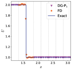
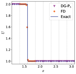
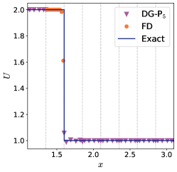
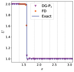
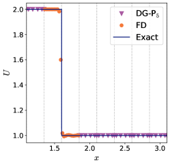
Figure 2: The step Burgers problem at $t_{f}=1.5$ using a DG-P₅ scheme hybridized with a WCNS3 FD scheme. A third-order Adams-Bashforth time stepper is used and the mesh is moving at velocity $v_{g}^{x}=1.4$. Results in the top row are obtained using a time step size of $\Delta t=2.5\times 10^{-3}$ and in the bottom row using a time step size of $\Delta t=5\times 10^{-4}$. Going from left to right in the top row, the TCI used is the Persson TCI with $\alpha_{N}=3$, the Persson TCI with $\alpha_{N}=4$, and the RDMP TCI. Going from left to right in the bottom row, the TCI used is the Persson TCI with $\alpha_{N}=3$, the RDMP TCI, and Persson TCI with $\alpha_{N}=4$ along with the RDMP TCI.

6.2 General relativistic magnetohydrodynamics

In this section we present results of our DG-FD hybrid scheme when applied to various GRMHD test problems. The final test problem in this section is that of a single magnetized neutron star, demonstrating that our hybrid scheme is capable of simulating interesting relativistic astrophysics scenarios. We always use an HLL Riemann solver and typically the third-order strong-stability preserving Runge-Kutta (SSP RK3) time stepper [42]. However, we also compare a fifth-order Dormand-Prince method [66] to the RK3 method for some test problems. We mainly use the SSP RK3 stepper since this is a commonly used method when comparing shock capturing schemes. We also reconstruct the variables $\{\rho,p,Wv^{i},B^{i},\Phi\}$ using a monotonised central reconstruction scheme. We choose the resolution for the different problems by having the number of FD grid points be approximately equal to the number of grid points used by current production FD codes. Unless stated otherwise, we do not monitor $\tilde{B}^{i}$ with the Persson indicator since in most of the test cases we look at the magnetic field has discontinuities at or near the same place the fluid variables have discontinuities. All simulations use SpECTRE v2022.04.04 [33] and the input files are available as part of the arXiv version of this paper.

6.2.1 1d Smooth Flow

We consider a simple 1d smooth flow problem to test which of the limiters and troubled-cell indicators are able to solve a smooth problem without degrading the order of accuracy. A smooth density perturbation is advected across the domain with a velocity $v^{i}$. The analytic solution is given by

$$\rho =1+0.7\sin[k^{i}(x^{i}-v^{i}t)],$$ (131)

$$v^{i} =(0.8,0,0),$$ (132)

$$k^{i} =(1,0,0),$$ (133)

$$p =1,$$ (134)

$$B^{i} =(0,0,0),$$ (135)

and we close the system with an adiabatic equation of state,

$$p=\rho\epsilon\left(\Gamma-1\right),$$ (136)

where $\Gamma$ is the adiabatic index, which we set to 1.4. We use a domain given by $[0,2\pi]^{3}$, and apply periodic boundary conditions in all directions. The time step size is $\Delta t=2\pi/5120$ so that the spatial discretization error is larger than the time stepping error for all resolutions that we use.

Table 1: The errors and local convergence order for the smooth flow problem using different limiting strategies. Note that the limiter is not applied if the troubled-cell indicator determines the DG solution to be valid. We observe the expected convergence rate except when the solution is underresolved because too few elements are used or when the error is no longer dominated by the truncation error of the DG scheme.

• Method	$N_{x}$	$L_{2}(\mathcal{E}(\rho))$	$L_{2}$ Order
  DG-FD P3	02	3.50983e-1
  	04	1.22554e-1	01.52
  	08	3.72266e-4	08.36
  	16	1.61635e-5	04.53
  	32	9.76927e-7	04.05
  DG-FD P4	02	3.62426e-1
  	04	3.79759e-4	09.90
  	08	1.15193e-5	05.04
  	16	3.73055e-7	04.95
  DG-FD P5	2	3.45679e-01
  	4	2.23822e-05	13.91
  	8	3.18504e-07	06.13
  	16	5.08821e-09	05.97

We perform convergence tests at different DG orders and present the results in table 1. We show both the $L_{2}$ norm of the error and the convergence rate. The $L_{2}$ norm is defined as

$$L_{2}(u)=\sqrt{\frac{1}{M}\sum_{i=0}^{M-1}u_{i}^{2}},$$ (137)

where $M$ is the total number of grid points and $u_{i}$ is the value of $u$ at grid point $i$ and the convergence order is given by

$$L_{2}\;\mathrm{Order}=\log_{2}\left[\frac{L_{2}(\mathcal{E}_{N_{x}/2})}{L_{2}(\mathcal{E}_{N_{x}})}\right].$$ (138)

We find that when very few elements are used, the TCI decides the solution is not well represented on the DG grid. Although if we disable the FD scheme completely, we find the DG method is stable, we find it acceptable that the TCI switches to FD in order to ensure robustness. Ultimately we observe the expected rate of convergence for smooth problems.

6.2.2 1d Riemann Problems

One-dimensional Riemann problems are a standard test for any scheme that must be able to handle shocks. We will focus on the first, third, and fourth Riemann problems (RP1, RP3, RP4) of [67]. The setup is given in table 2. We perform simulations using an SSP RK3 and a Dormand-Prince 5 method with $\Delta t=5\times 10^{-4}$. In the top left panels of figures 3-5 we show the rest mass density $\rho$ at $t_{f}=0.4$, the bottom left panels show $B^{y}$, while the right panels show the difference between the analytic and numerical solution. The thin black curve is the analytic solution obtained using the Riemann solver of [68]. An ideal fluid equation of state (136) is used.

Table 2: The initial conditions for Riemann Problems 1, 3, and 4 of [67]. The domain is $x\in[-0.5,0.5]$, the final time is $t_{f}=0.4$, and an ideal fluid equation of state is used with an adiabatic index of 2 for Riemann Problem 1 and $5/3$ for Riemann Problems 3 and 4.

• Problem		$\rho$	$p$	$v^{i}$	$B^{i}$
  RP 1	$x<0$	1.000	0001.0	$(\phantom{-}0.0\hbox{\phantom{\footnotesize\rm 0}}\hbox{\phantom{\footnotesize\rm 0}},0,0)$	$(\hbox{\phantom{\footnotesize\rm 0}}0.5,\phantom{-}1.0,\phantom{-}0.0)$
  	$x\geq 0$	0.125	0000.1	$(\phantom{-}0.0\hbox{\phantom{\footnotesize\rm 0}}\hbox{\phantom{\footnotesize\rm 0}},0,0)$	$(\hbox{\phantom{\footnotesize\rm 0}}0.5,-1.0,\phantom{-}0.0)$
  RP 3	$x<0$	1.000	1000.0	$(\phantom{-}0.0\hbox{\phantom{\footnotesize\rm 0}}\hbox{\phantom{\footnotesize\rm 0}},0,0)$	$(10.0,\phantom{-}7.0,\phantom{-}7.0)$
  	$x\geq 0$	1.000	0000.1	$(\phantom{-}0.0\hbox{\phantom{\footnotesize\rm 0}}\hbox{\phantom{\footnotesize\rm 0}},0,0)$	$(10.0,\phantom{-}0.7,\phantom{-}0.7)$
  RP 4	$x<0$	1.000	0000.1	$(\phantom{-}0.999,0,0)$	$(10.0,\phantom{-}7.0,\phantom{-}7.0)$
  	$x\geq 0$	1.000	0000.1	$(-0.999,0,0)$	$(10.0,-7.0,-7.0)$

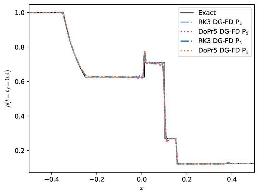
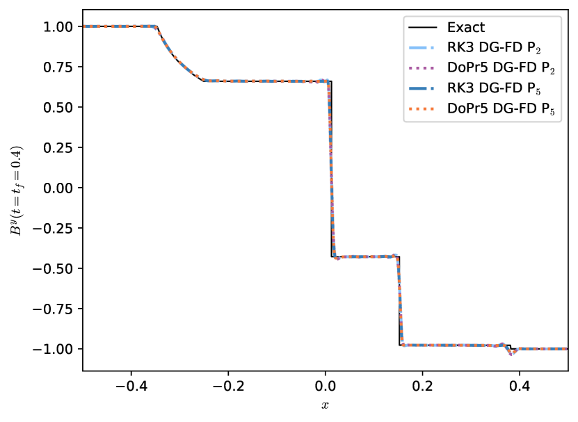
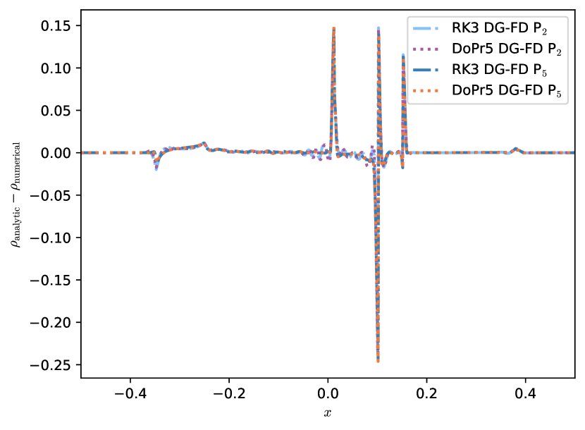
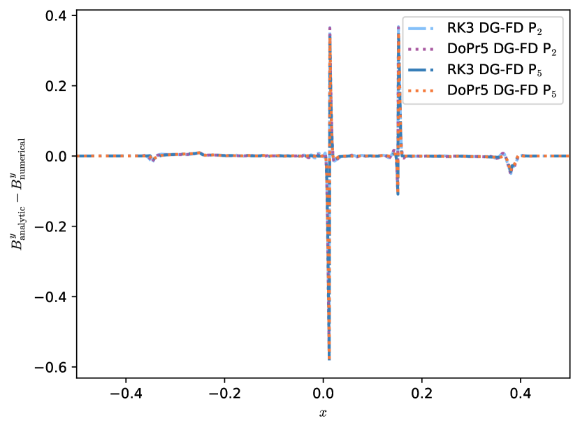
Figure 3: Results from Riemann Problem 1 of [67] using a P₅ (64 elements) and P₂ (128 elements) DG-FD hybrid scheme with an SSP RK3 and Dormand-Prince 5 time stepper. All results are at the final time $t=0.4$. The top left panel shows the rest mass density $\rho$, the bottom left the magnetic field $B^{y}$, and the right panels show the difference between the analytic and numerical solution. The P₅ scheme is able to resolve the discontinuities just as well as the P₂ scheme, while also admitting fewer unphysical oscillations away from the discontinuities.

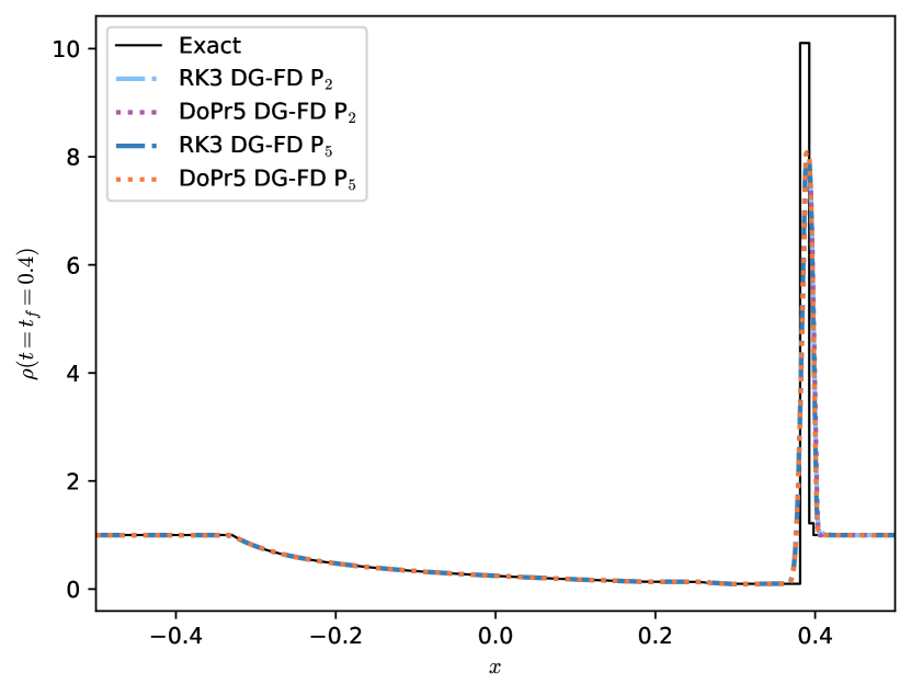
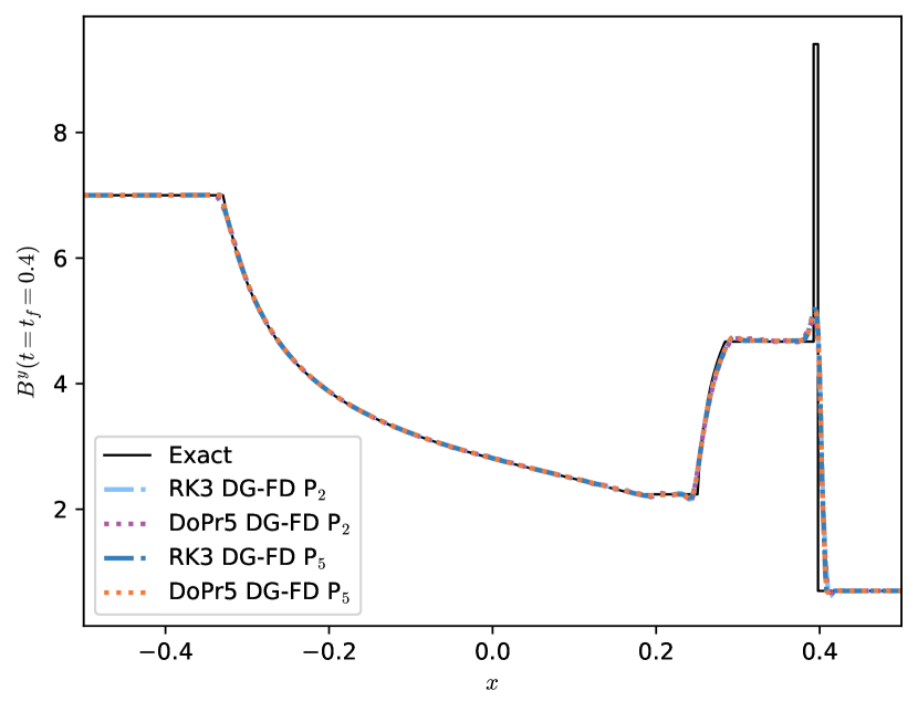
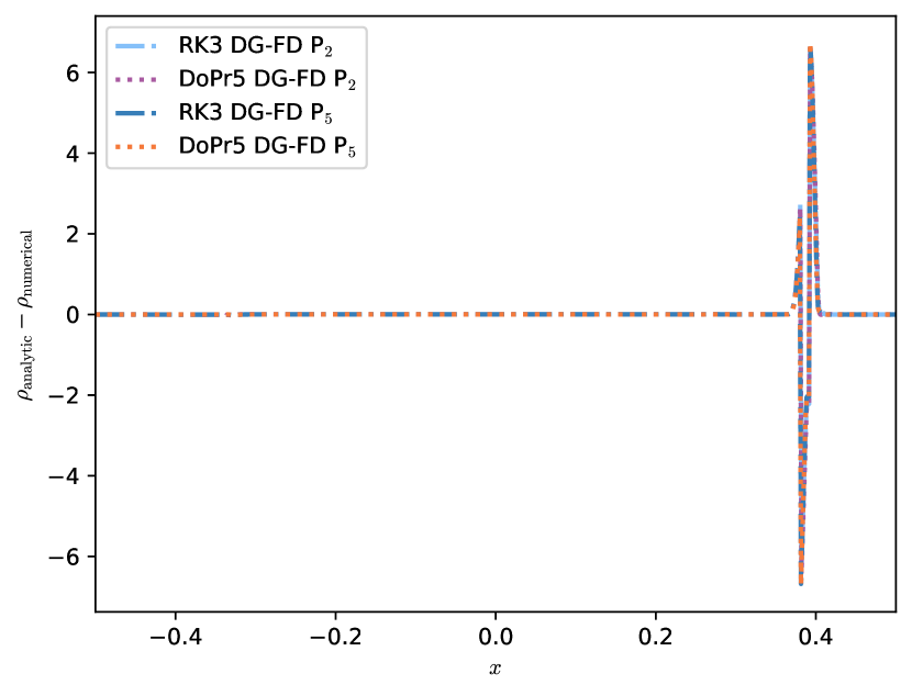
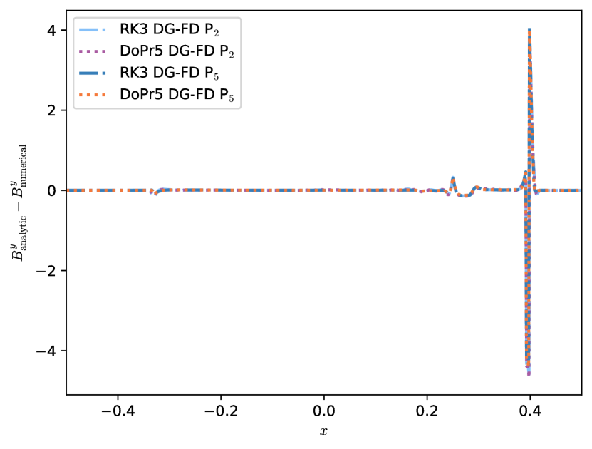
Figure 4: Results from Riemann Problem 3 of [67] using a P₅ (64 elements) and P₂ (128 elements) DG-FD hybrid scheme with an SSP RK3 and Dormand-Prince 5 time stepper. All results are at the final time $t=0.4$. The top left panel shows the rest mass density $\rho$, the bottom left the magnetic field $B^{y}$, and the right panels show the difference between the analytic and numerical solution. The P₅ scheme is able to resolve the discontinuities just as well as the P₂ scheme, while also admitting fewer unphysical oscillations away from the discontinuities.

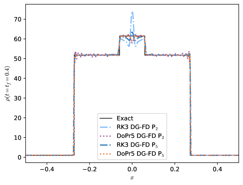
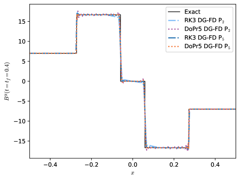
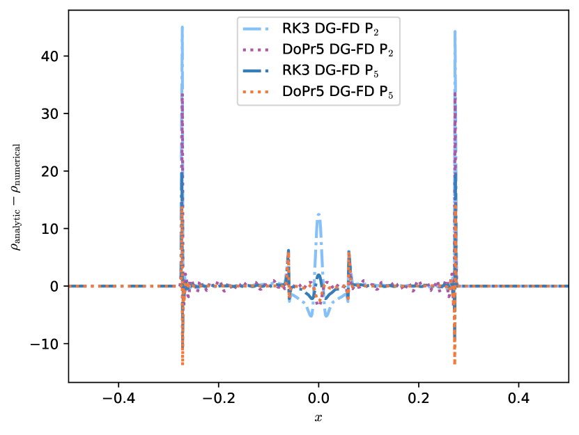
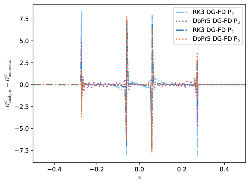
Figure 5: Results from Riemann Problem 4 of [67] using a P₅ (64 elements) and P₂ (128 elements) DG-FD hybrid scheme with an SSP RK3 and Dormand-Prince 5 time stepper. All results are at the final time $t=0.4$. The top left panel shows the rest mass density $\rho$, the bottom left the magnetic field $B^{y}$, and the right panels show the difference between the analytic and numerical solution. The P₅ scheme is able to resolve the discontinuities just as well as the P₂ scheme, while also admitting fewer unphysical oscillations away from the discontinuities.

Impressively, the DG-FD hybrid scheme actually has fewer oscillations when going to higher order. In the right panels of figures 3-5 we plot the error of the numerical solution using a P₂ DG-FD scheme with 128 elements and a P₅ DG-FD scheme with 64 elements. We see that the P₅ hybrid scheme actually has fewer oscillations than the P₂ scheme, while resolving the discontinuities equally well. We attribute this to the troubled-cell indicators triggering earlier when a higher polynomial degree is used since discontinuities entering an element rapidly dump energy into the high modes. While the optimal order is almost certainly problem-dependent, given that current numerical relativity codes are mostly second order, achieving sixth order in the smooth regions is promising. The SSP RK3 time stepper seems to generally result in fewer oscillations than the Dormand-Prince 5 time stepper. This could stem from the Dormand-Prince stepper not being strong stability preserving. We leave a detailed comparison of different time integration schemes to future work.

6.2.3 2d Cylindrical Blast Wave

A standard test problem for GRMHD codes is the cylindrical blast wave [69, 70] where a magnetized fluid initially at rest in a constant magnetic field along the $x$-axis is evolved. The fluid obeys the ideal fluid equation of state with $\Gamma=4/3$. The fluid begins in a cylindrically symmetric configuration, with hot, dense fluid in the region with cylindrical radius $r<0.8$ surrounded by a cooler, less dense fluid in the region $r>1$. The initial density $\rho$ and pressure $p$ of the fluid are

$$\rho(r<0.8) =10^{-2},$$ (139)

$$\rho(r>1.0) =10^{-4},$$ (140)

$$p(r<0.8) =1,$$ (141)

$$p(r>1.0) =5\times 10^{-4}.$$ (142)

In the region $0.8\leq r\leq 1$, the solution transitions continuously and exponentially (i.e., transitions such that the logarithms of the pressure and density are linear functions of $r$). The fluid begins threaded with a uniform magnetic field with Cartesian components

$$(B^{x},B^{y},B^{z})=(0.1,0,0).$$ (143)

The magnetic field causes the blast wave to expand non-axisymmetrically. For all simulations we use a time step size $\Delta t=10^{-2}$ and an SSP RK3 time integrator.

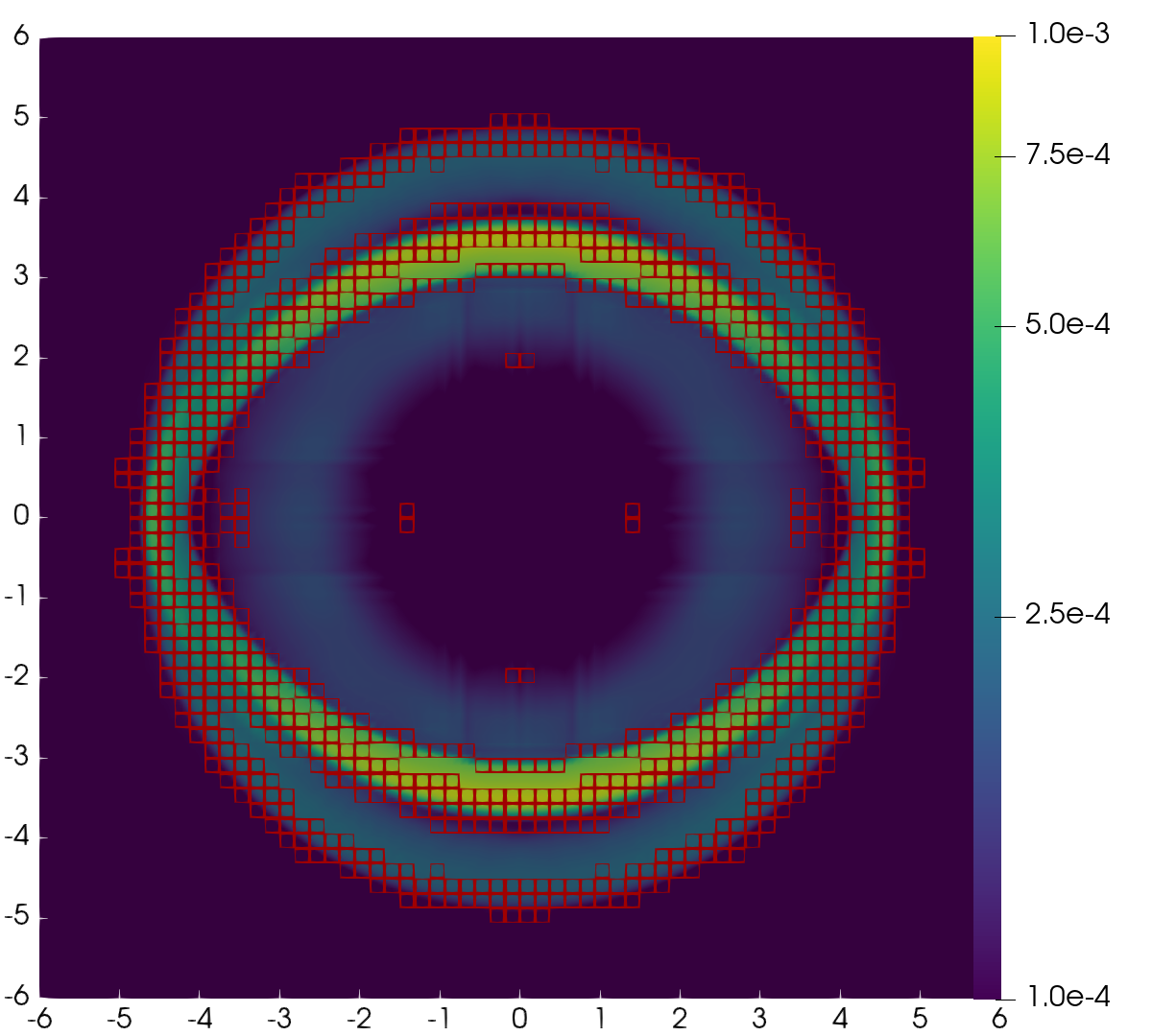
DG-FD, P₂, $64^{2}$ elements

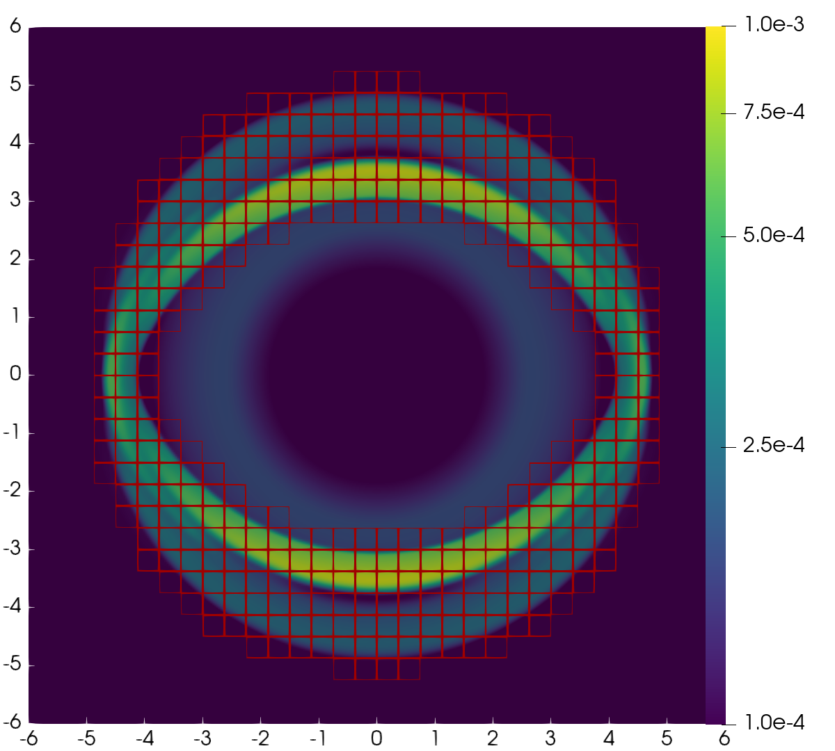
DG-FD, P₅, $32^{2}$ elements

Figure 6: Cylindrical blast wave $\rho$ at $t=4$ showing the results of the using the DG-FD hybrid scheme with $64\times 64$ P₂ elements (left) and $32\times 32$ P₅ elements (right). The regions surrounded by maroon squares have switched from DG to FD.

We evolve the blast wave to time $t=4.0$ on a grid of $64\times 64\times 1$ elements covering a cube of extent $[-6,6]^{3}$ using a P₂ DG-FD scheme and on a grid of $32\times 32\times 1$ using a P₅ DG-FD scheme. With these choices the resolution when using FD everywhere is comparable to what FD codes use for this test. We apply periodic boundary conditions in all directions, since the explosion does not reach the outer boundary by $t=4.0$. Figure 6 shows the logarithm of the rest-mass density at time $t=4.0$, at the end of evolutions using the P₂ (left) and P₅ (right) DG-FD schemes. The increased resolution of a high-order scheme is clear when comparing the P₂ and P₅ solutions in the interior region of the blast wave. It is not clear that going to even higher order would be useful in this problem since to maintain the same time step size we would need to decrease the number of elements. Furthermore, as we can already see by comparing the P₂ and P₅ schemes, a greater area of the P₅ solution is using FD, though it is difficult to determine what overall effect this has, especially since high-order FD schemes could be used. We show the percentage of elements using FD instead of DG at the final time in table 3. As expected, the percentage of elements using FD decreases as the number of elements is increased.

Table 3: The percentage of elements using FD at the final time of the cylindrical blast wave simulation

• Method	Domain	Percent Using FD
  DG-FD P2	0322	036.7%
  	0642	022.9%
  	01282	07.9%
  DG-FD P5	0162	057.8%
  	0322	035.9%
  	0642	021.8%

6.2.4 2d Magnetic Rotor

The second 2-dimensional test problem we study is the magnetic rotor problem originally proposed for non-relativistic MHD [71, 72] and later generalized to the relativistic case [73, 74]. A rapidly rotating dense fluid cylinder is inside a lower density fluid, with a uniform pressure and magnetic field everywhere. The magnetic braking will slow down the rotor over time, with an approximately 90 degree rotation by the final time $t=0.4$. We use a domain of $[-0.5,0.5]^{3}$ and a time step size $\Delta t=10^{-3}$ and an SSP RK3 time integrator. An ideal fluid equation of state with $\Gamma=5/3$ is used, and the following initial conditions are imposed:

$$p =1$$ (144)

$$B^{i} =(1,0,0)$$ (145)

$$v^{i} =\left\{\begin{array}[]{ll}(-y\Omega,x\Omega,0),&\mathrm{if}\;r\leq R_{\mathrm{rotor}}=0.1\\ (0,0,0),&\mathrm{otherwise},\end{array}\right.$$ (148)

$$\rho =\left\{\begin{array}[]{ll}10,&\mathrm{if}\;r\leq R_{\mathrm{rotor}}=0.1\\ 1,&\mathrm{otherwise},\end{array}\right.$$ (151)

with angular velocity $\Omega=9.95$. The choice of $\Omega$ and $R_{\mathrm{rotor}}=0.1$ guarantees that the maximum velocity of the fluid (0.995) is less than the speed of light. We impose periodic boundary conditions.

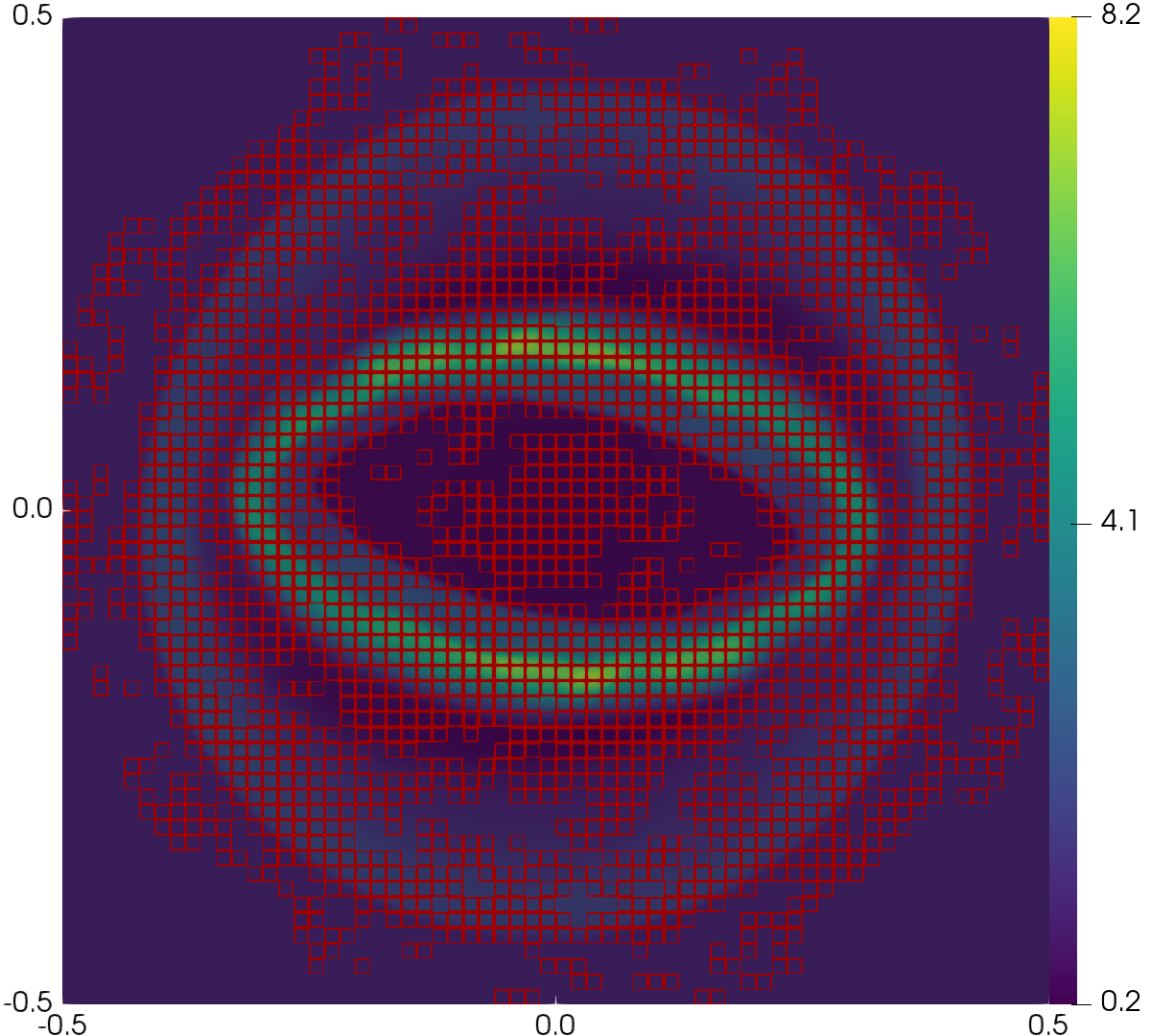
DG-FD, P₂, $64^{2}$ elements

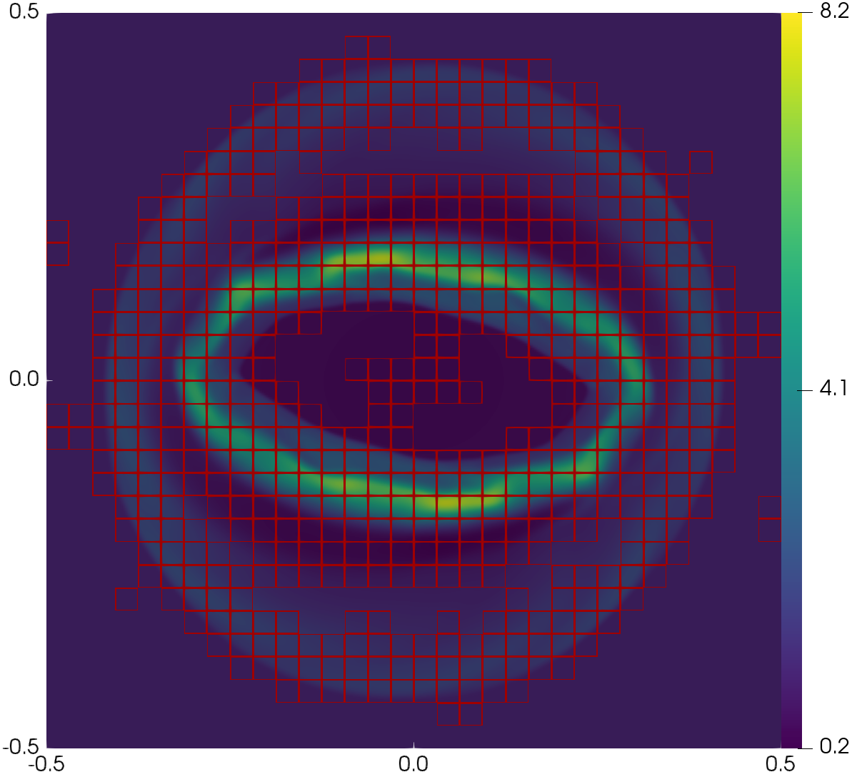
DG-FD, P₅, $32^{2}$ elements

Figure 7: Magnetic rotor $\rho$ at $t=0.4$ showing the results of the using the DG-FD hybrid scheme with $64\times 64$ P₂ elements (left) and $32\times 32$ P₅ elements (right). The regions surrounded by maroon squares have switched from DG to FD.

We show the results of our evolutions using $64\times 64$ P₂ elements (left) and $32\times 32$ P₅ elements (right) in figure 7. Again, the DG-FD hybrid scheme is robust and accurate, though a fairly large number of cells end up being marked as troubled in this problem. However, using FD in more elements is not something we view as inherently bad, since we favor robustness in realistic simulations. The process of tweaking parameters and restarting simulations is both time consuming and frustrating, and so giving up some efficiency for robustness is preferable in general .

6.2.5 2d Magnetic Loop Advection

The last 2-dimensional test problem we study is magnetic loop advection problem [75]. A magnetic loop is advected through the domain until it returns to its starting position. We use an initial configuration very similar to [40, 76, 77, 78], where

$$\rho =1$$ (152)

$$p =3$$ (153)

$$v^{i} =(1/1.2,1/2.4,0)$$ (154)

$$B^{x} =\left\{\begin{array}[]{ll}-A_{\mathrm{loop}}y/R_{\mathrm{in}},&\mathrm{if}\;r\leq R_{\mathrm{in}}\\ -A_{\mathrm{loop}}y/r,&\mathrm{if}\;R_{\mathrm{in}}<r<R_{\mathrm{loop}}\\ 0,&\mathrm{otherwise},\end{array}\right.$$ (158)

$$B^{y} =\left\{\begin{array}[]{ll}A_{\mathrm{loop}}x/R_{\mathrm{in}},&\mathrm{if}\;r\leq R_{\mathrm{in}}\\ A_{\mathrm{loop}}x/r,&\mathrm{if}\;R_{\mathrm{in}}<r<R_{\mathrm{loop}}\\ 0,&\mathrm{otherwise},\end{array}\right.$$ (162)

with $R_{\mathrm{loop}}=0.3$, $R_{\mathrm{in}}=0.001$, and an ideal gas equation of state with $\Gamma=5/3$. The computational domain is $[-0.5,0.5]^{3}$ with $64\times 64\times 1$ elements and periodic boundary conditions being applied everywhere. The final time for one period is $t=2.4$. For all simulations we use a time step size $\Delta t=10^{-3}$ and an SSP RK3 time integrator. Since the fluid variables are smooth in this problem, we apply the Persson TCI to the Euclidean magnitude of $\tilde{B}^{i}$ in elements where the maximum value of the magnitude is above $10^{-5}$.

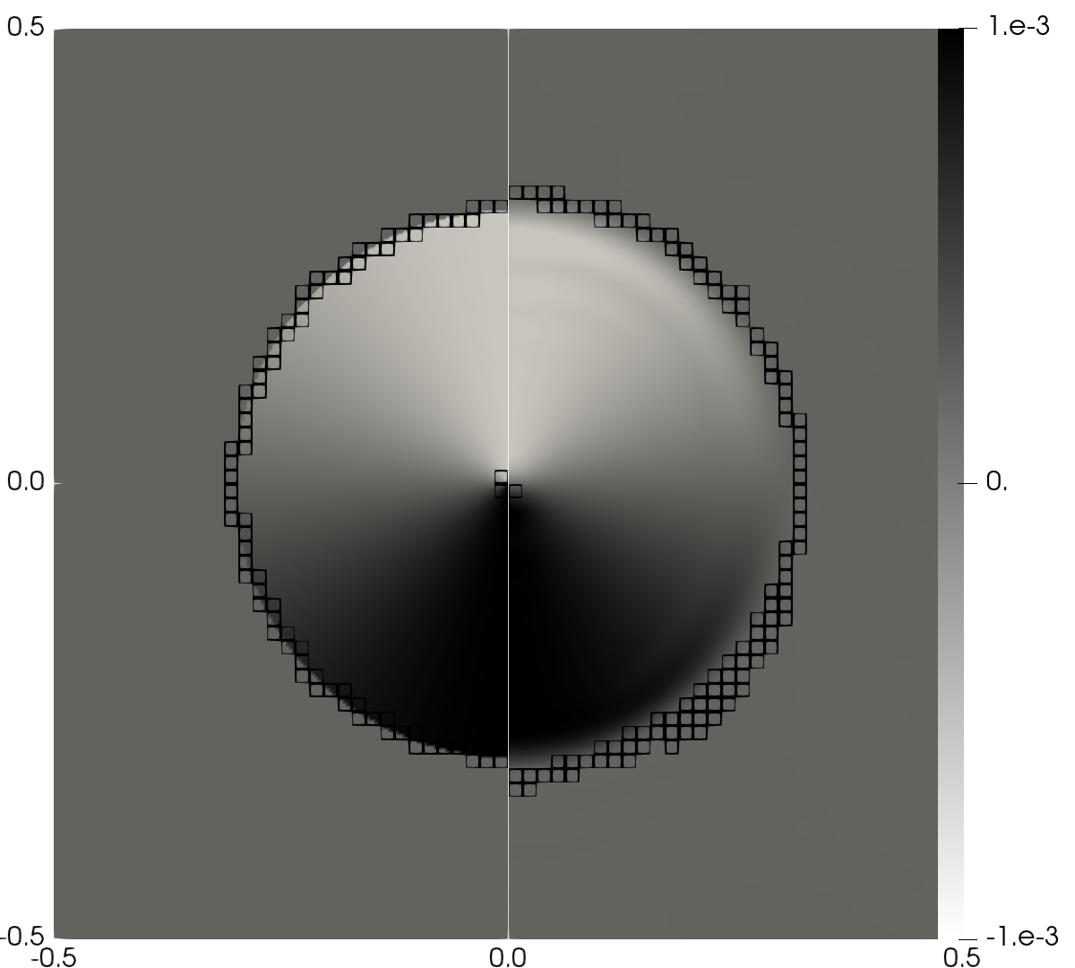
DG-FD, P₂, $64^{2}$ elements

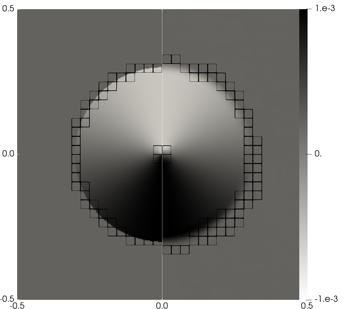
DG-FD, P₅, $32^{2}$ elements

Figure 8: $B^{x}$ for the magnetic loop advection problem. The left half of each plot is at the initial time, while the right half is after one period ($t=2.4$). We show the results of the using the DG-FD hybrid scheme with $64\times 64$ P₂ elements (left) and $32\times 32$ P₅ elements (right). The regions surrounded by black squares have switched from DG to FD.

In figure 8 we plot the magnetic field component $B^{x}$ at $t=0$ on the left half of each plot and after one period $t=2.4$ on the right half of each plot. In the left panel of figure 8 we show the result using a P₂ DG-FD scheme and in the right panel of figure 8 using a P₅ DG-FD scheme. The P₅ scheme resolves the smooth parts of the solution more accurately than the P₂ scheme, as is to be expected. Finally, in figure 9 we plot the divergence cleaning field $\Phi$ at the final time $t=2.4$. We do not observe any artifacts appearing in the divergence cleaning field at the interfaces between the DG and FD solvers, demonstrating that the divergence cleaning properties of the system are not adversely affected by using two different numerical methods.

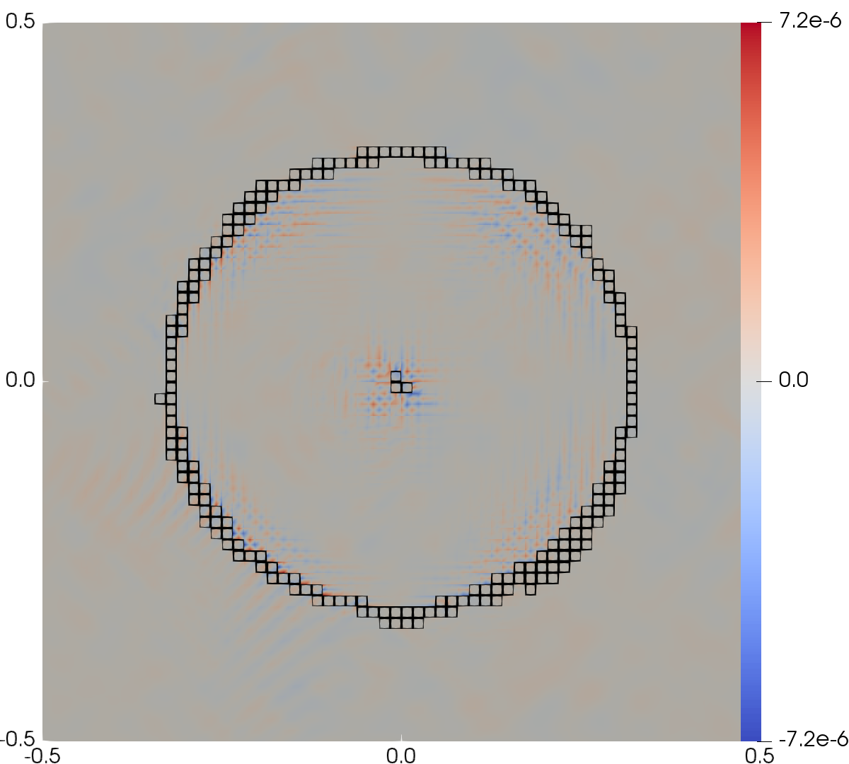
DG-FD, P₂, $64^{2}$ elements

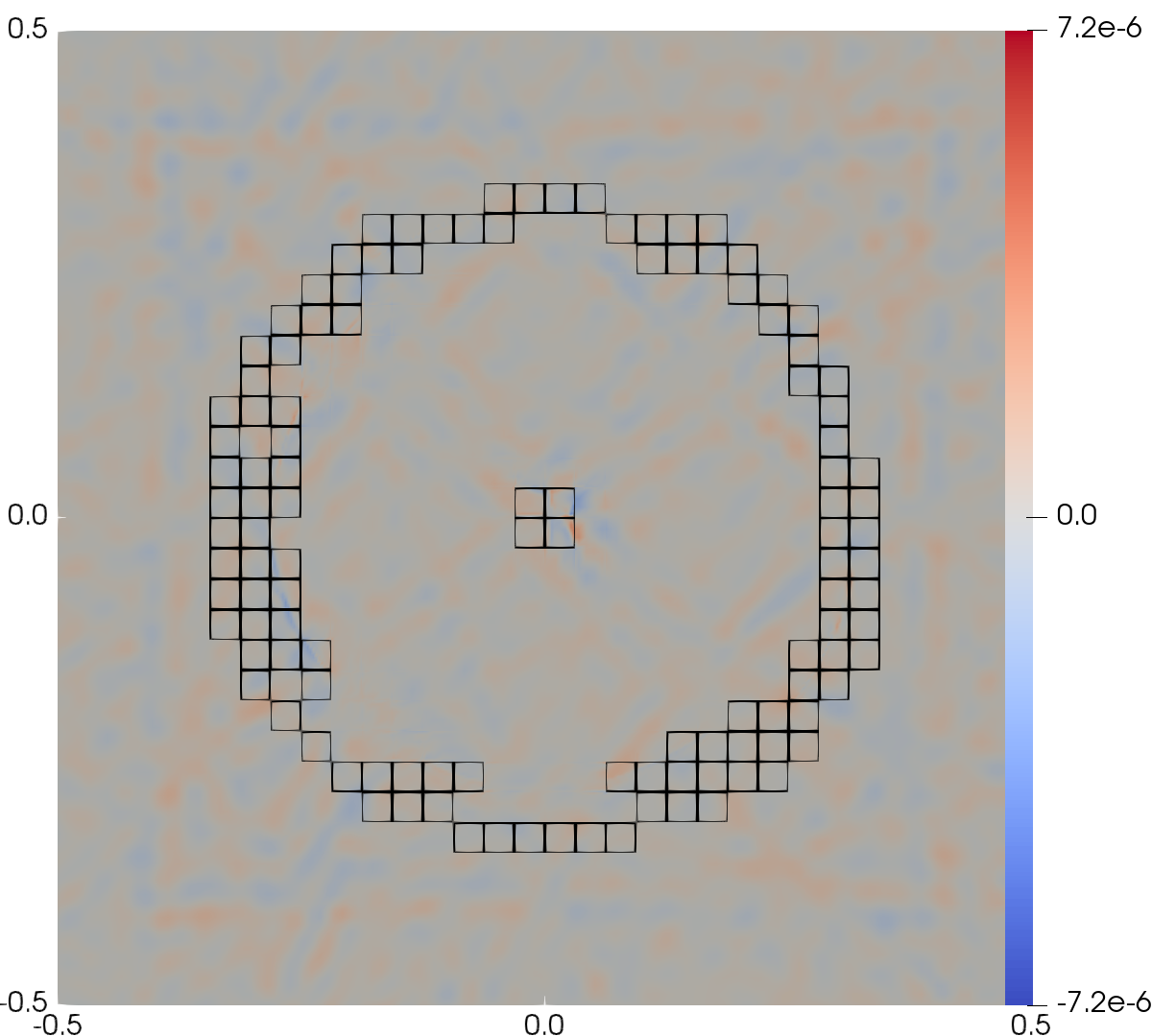
DG-FD, P₅, $32^{2}$ elements

Figure 9: The divergence cleaning field $\Phi$ for the magnetic loop advection problem after one period ($t=2.4$). We show the results of the using the DG-FD hybrid scheme with $64\times 64$ P₂ elements (left) and $32\times 32$ P₅ elements (right). The regions surrounded by black squares have switched from DG to FD.

6.2.6 TOV star

A rigorous 3d test case in general relativity is the evolution of a Tolman-Oppenheimer-Volkoff (TOV) star [79, 80]. In this section we study evolutions of both non-magnetized and magnetized TOV stars. We adopt the same configuration as in [81]. Specifically, we use a polytropic equation of state,

$$p(\rho)=K\rho^{\Gamma}$$ (163)

with the polytropic exponent $\Gamma=2$, polytropic constant $K=100$, and a central density $\rho_{c}=1.28\times 10^{-3}$. For the magnetized case, we choose a magnetic field given by a vector potential

$$A_{\phi}=A_{b}\left(x^{2}+y^{2}\right)\max\left(p-p_{\mathrm{cut}},0\right)^{n_{s}},$$ (164)

with $A_{b}=2500$, $p_{\mathrm{cut}}=0.04p_{\max}$, and $n_{s}=2$. This configuration yields a magnetic field strength in CGS units

$$|B_{\mathrm{CGS}}|=\sqrt{b^{2}}\times 8.352\times 10^{19}\,\mathrm{G},$$ (165)

of $|B_{\mathrm{CGS}}|=1.03\times 10^{16}\,\mathrm{G}$. The magnetic field is only a perturbation to the dynamics of the star, since $(p_{\mathrm{mag}}/p)(r=0)\sim 5\times 10^{-5}$. However, evolving the field stably and accurately can be challenging. The magnetic field corresponding to the vector potential in (164) in the magnetized region is given by

$$B^{x} =\frac{1}{\sqrt{\gamma}}\frac{xz}{r}A_{b}n_{s}(p-p_{\mathrm{cut}})^{n_{s}-1}\partial_{r}p,$$ (166)

$$B^{y} =\frac{1}{\sqrt{\gamma}}\frac{yz}{r}A_{b}n_{s}(p-p_{\mathrm{cut}})^{n_{s}-1}\partial_{r}p,$$ (167)

$$B^{z} =-\frac{A_{b}}{\sqrt{\gamma}}\left[2(p-p_{\mathrm{cut}})^{n_{s}}+\frac{x^{2}+y^{2}}{r}n_{s}(p-p_{\mathrm{cut}})^{n_{s}-1}\partial_{r}p\right],$$ (168)

and at $r=0$ is

$$B^{x} =0,$$ (169)

$$B^{y} =0,$$ (170)

$$B^{z} =-\frac{A_{b}}{\sqrt{\gamma}}2(p-p_{\mathrm{cut}})^{n_{s}}.$$ (171)

We perform all evolutions in full 3d with no symmetry assumptions and in the Cowling approximation, i.e., we do not evolve the spacetime. To match the resolution usually used in FD/FV numerical relativity codes, we use a domain $[-20,20]^{3}$ with a base resolution of six P₅ DG elements. This choice means we have approximately 32 FD grid points covering the star’s diameter at the lowest resolution, 64 when using twelve P₅ elements, and 128 grid points when using 24 P₅ elements. In all cases we set $\rho_{\mathrm{atm}}=10^{-15}$ and $\rho_{\mathrm{cutoff}}=1.01\times 10^{-15}$. We do not run any simulations using a P₂ DG-FD hybrid scheme since the P₅ scheme has proven to be more accurate and robust in all test cases so far.

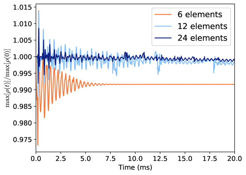
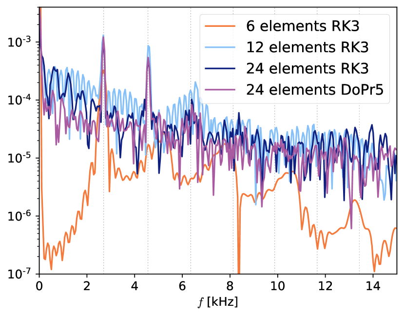
Figure 10: A plot of $\max[\rho(t)]/\max[\rho(0)]$ at three different resolution (left panel) for the non-magnetized TOV star. The 6-element simulation uses FD throughout the interior of the star, while 12- and 24-element simulations use DG. The maximum density in the 6-element case drifts down at early times because of the low resolution and the relatively low accuracy of using FD at the center. The power spectrum of the maximum density for the three different resolution is plotted in the right panel. The vertical dashed lines correspond to the known frequencies in the Cowling approximation [82]. When the high-order DG scheme is used, more oscillation frequencies are resolved. We also show the spectrum from a simulation using a fifth-order Dormand-Prince time stepper.

In the left panel of figure 10 we show the maximum rest mass density over the grid divided by the maximum density at $t=0$ for the non-magnetized TOV star. The 6-element simulation uses FD throughout the interior of the star because the corners of the inner elements are in vacuum. In comparison, the 12- and 24-element simulations use the unlimited P₅ DG solver throughout the star interior. The increased “noise” in the 12- and 24-element data actually stems from the higher oscillation modes in the star [82] that are induced by numerical error. In the right panel of figure 10 we plot the power spectrum using data at the three different resolutions. The 6-element simulation only has one mode resolved, while 12 elements resolve two modes well, and the 24-element simulation resolves three modes well. Additionally, we plot the power spectrum from a 24-element simulation using a fifth-order Dormand-Prince time stepper instead of the strong stability preserving third-order Runge-Kutta method. Increasing the time stepper order does not increase the number of radial modes resolved, demonstrating that it is the spatial resolution that is the limiting factor.

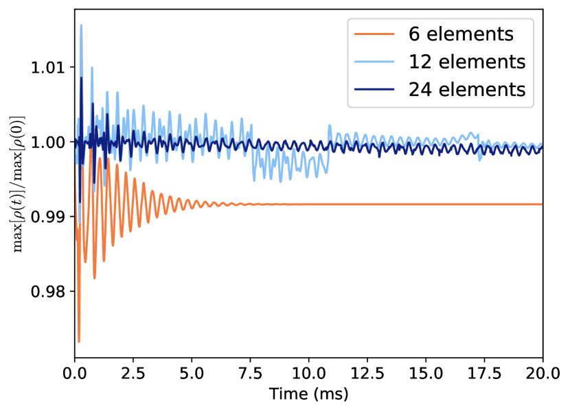
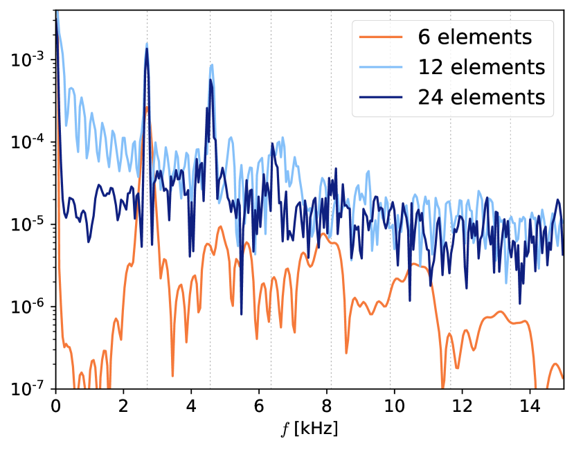
Figure 11: A plot of $\max[\rho(t)]/\max[\rho(0)]$ at three different resolution (left panel) for the magnetized TOV star. The 6-element simulation uses FD throughout the interior of the star, while 12- and 24-element simulations use DG. The maximum density in the 6-element case drifts down at early times because of the low resolution and the relatively low accuracy of using FD at the center. The power spectrum of the maximum density for the three different resolution is plotted in the right panel. The vertical dashed lines correspond to the known frequencies in the Cowling approximation (which are the same as the non-magnetized case as the magnetic field is a small perturbation on the dynamics). When the high-order DG scheme is used, more oscillation frequencies are resolved.

We show the normalized maximum rest mass density over the grid for the magnetized TOV star in the left panel of figure 11. Overall the results are nearly identical to the non-magnetized case. One notable difference is the decrease in the 12-element simulation between 7.5ms and 11ms, which occurs because the code switches from DG to FD at the center of the star at 7.5ms and back to DG at 11ms. Nevertheless, the frequencies are resolved just as well for the magnetized star as for the non-magnetized case, as can be seen in the right panel of figure 11 where we plot the power spectrum. Specifically, we are able to resolve the three largest modes with our P₅ DG-FD hybrid scheme. To the best of our knowledge, these are the first simulations of a magnetized neutron star using high-order DG methods.

6.2.7 Rotating neutron star

As a final test case we simulate a uniformly rotating neutron star with ratio of polar to equatorial radius of 0.7, similar to that of [82]. The initial data is constructed using the method described in [83, 84]. We use the same polytropic equation of state as for the TOV star evolution. In the left panel of figure 12 we show the maximum of the rest mass density for the same three resolutions used for the TOV star simulations. The lowest resolution uses FD throughout the star and sees a rapid decay in the density. The 12-element simulation uses DG throughout most of the interior of the star and so sees significant less decay in the density. The 24-element simulation uses DG everywhere in the interior of the star and sees less than a 0.1% decay in the density over 20ms. To further test convergence we plot the maximum density of a 1ms long 24-element and 48-element simulation in the right panel of figure 12. The oscillations continue to decrease with increasing resolution. We attribute the decay in the maximum density at lower resolutions to the dissipative nature of FD schemes, consistent with the rapid reduction in decay of the maximum density when switching to DG and increasing the resolution. These are also the first simulations of a rotating neutron star using high-order DG methods.

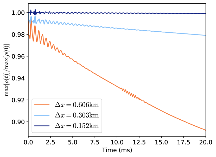
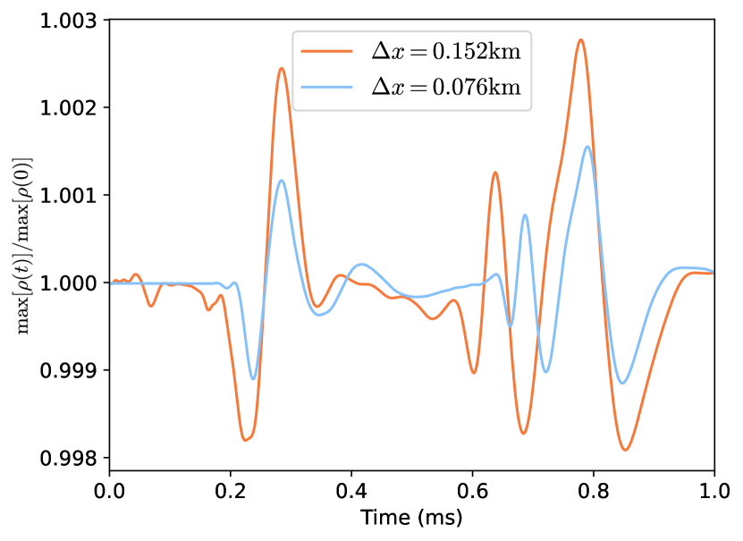
Figure 12: The left panel shows $\max[\rho(t)]/\max[\rho(0)]$ at three different resolution for the uniformly rotating neutron star. The 6-element simulation uses FD throughout the interior of the star, the 12-element simulation uses mostly DG in the stellar interior, and the 24-element simulations use DG everywhere except the stellar surface. The right panel shows $\max[\rho(t)]/\max[\rho(0)]$ for a shorter period of time but at very high resolutions, 24 elements and 48 elements. Increasing from 24 to 48 elements further reduces oscillations in the maximum density.

7 Conclusions

In this paper we gave a detailed description of our DG-FD hybrid method that can successfully solve challenging relativistic astrophysics test problems like the simulation of a magnetized or rotating neutron star. Our method combines an unlimited DG solver with a conservative FD solver. Alternatively, this can be thought of as taking a standard FD code in numerical relativity and compressing the data to a DG grid wherever the solution is smooth. The DG solver is more efficient than the FD solver since no reconstruction is necessary and fewer Riemann problems need to be solved. In theory a speedup of about eight is achievable, though we have not optimized our code SpECTRE [33] enough and so we find in practice a speedup of about two to three when comparing the hybrid method to using FD everywhere. The basic idea of the hybrid scheme is similar to [10, 11, 12, 13]. An unlimited DG solver is used wherever a troubled-cell indicator deems the DG solution admissible, while a FD solver is used elsewhere. Unlike classical limiting strategies like WENO which attempt to filter out unphysical oscillations, the hybrid scheme prevents spurious oscillations from entering the solution. This is achieved by retaking any time step using a robust high-resolution shock-capturing conservative FD where the DG solution was inadmissible, either because the DG scheme produced unphysical results like negative densities or because a numerical criterion like the percentage of power in the highest modes deemed the DG solution bad. Our DG-FD hybrid scheme was used to perform what is to the best of our knowledge the first ever simulations of a magnetized TOV star and rotating neutron star using DG methods. In the future we plan to extend the hybrid scheme to curved meshes, simulations in full general relativity where the metric is evolved, and to use positivity-preserving adaptive-order FD methods in order to maintain the highest order possible even when using FD instead of DG.

Appendix A Curved hexahedral elements and moving meshes

We have not yet implemented support for curved hexahedral meshes into SpECTRE. However, we have given careful consideration on how they could be implemented. In this appendix we discuss two possible implementations, one that requires many additional ghost cells with dimension-by-dimension reconstruction, and one that requires multidimensional reconstruction but no additional ghost cells.

Support for curved hexahedral or rectangular meshes can be achieved by combining the DG scheme with a multipatch or multidomain FD scheme. We will discuss only the 2d case, since the 3d case has more tedious bookkeeping, but otherwise is a straightforward extension. As a concrete example, we consider a 2d disk made out of a square surrounded by four wedges as shown in figure 13. We focus on an element at the top right corner of the central square and its neighbors, highlighted by the dashed squared in figure 13. We will first discuss how to handle the boundaries when a pair of neighboring elements are using the FD scheme, and then consider the case when one element is using DG and the other FD.

Figure 13: A 2d disk made out of a central square surrounded by four wedges. In the text we describe the method of handling intercell fluxes for the elements inside the dashed square.

In figure 14 we illustrate the domain setup, showing the subcell center points as circles in the two elements of interest. The diamonds in left panel of figure 14 represent the ghost cells needed for reconstruction to the element boundary in the element on the right. We use diagonal dotted lines to trace out lines of constant reference coordinates in the element on the right and dashed lines in the element on the left. Notice that the dashed and dotted lines intersect on the element boundary. This is because the mapping from the reference frame is continuous across element boundaries and allows us to have a conservative scheme using centered stencils even in the multipatch case.

An illustration of the ghost points needed for the FD scheme where neighboring elements do not have aligned coordinate axes in their reference frames. Circles denote the cell-center FD points in the elements, and diamonds denote the ghost cells needed for reconstruction in the element on the right. The diagonal dotted lines trace out lines of constant reference coordinates in the element on the right, and dashed lines in the element on the left. Notice that the dashed and dotted lines intersect on the element boundary.

An illustration of extending the FD element by additional cells in order to support high-order reconstruction to arbitrary points inside the element, as discussed in the text. The additional cells for the central element are shown as purple triangles. These additional cells are evolved alongside the cells inside the element.

An illustration of the first stage of the reconstruction to the ghost cells needed by the neighboring element on the right. The central element reconstructs the solution to a line in the reference coordinates, followed by a second reconstruction to the ghost cells that fall on the line (not shown for simplicity).

Figure 14: An illustration of the multipatch or multidomain FD reconstruction needed to support curved meshes. We show a 2d example for simplicity. The 3d case is a tedious but otherwise straightforward generalization.

Since we are unable to interpolate to the ghost cells shown in the left panel of figure 14 with centered stencils, one option is to use non-centered stencils. Using non-centered stencils was explored in reference [91], which did not find any instabilities from the use of such stencils in their test cases. Another option is to use reconstruction methods for unstructured meshes (see, for example, [92, 93, 94, 95, 96, 97] and references therein), though this adds significant conceptual and technical overhead. Another option is adding additional subcells that overlap with the neighboring elements to allow the use of centered reconstruction schemes to interpolate to the ghost cells. These additional subcells are shown as triangles in the middle panel of figure 14. We can now do two reconstructions to reconstruct the ghost cells. First, we reconstruct along one reference axis of the central element as shown by the squares in the right panel of figure 14. Next we reconstruct along the other direction, which is illustrated by the dotted vertical line in the right panel of figure 14.

In order to maintain conservation between elements, we need to define a unique left and right state at the boundary of the elements. A unique state can be obtained by using the average of the reconstructed variables from the diagonal and horizontal stencils in figure 14. That is, we use the average of the result obtained from reconstruction in each element for the right and left states when updating any subcells that need the numerical flux on the element boundaries. Recall that when using a second-order FD derivative the semi-discrete evolution equations are (we only show 1d for simplicity since it is sufficient to illustrate our point)

$$\partial_{t}u+\frac{\partial\xi}{\partial x}\left(\frac{\hat{F}^{x}_{\underline{i}+1/2,\underline{j}}-\hat{F}^{x}_{\underline{i}-1/2},\underline{j}}{\Delta\xi}\right)=S.$$ (172)

Thus, as long as all cells that share the boundary on which the numerical fluxes are defined use the same numerical flux, the scheme is conservative. When using higher-order derivative approximations the fluxes away from the cell boundaries are also needed. In the case of the element boundaries we are considering, we do not have a unique solution in the region of overlap (e.g. the region covered by the purple triangles in the middle panel of figure 14) where we compute the fluxes. As a result, we do not know if using high-order FD derivatives would violate conservation at the element boundaries. However, if the solution is smooth in this region, small violations of conservation are not detrimental, and if a discontinuity is passing through the boundary a second-order FD derivative should be used anyway.

Another method of doing reconstruction at locations where the coordinate axes do not align is described in [98] for finite-volume methods. This same approach should be applicable to FD methods. Whether adding ghost zones or using unstructured mesh reconstruction is easier to implement and more efficient is unclear and will need to be tested.

Appendix B Integration weights

The standard weights available in textbooks assume the abscissas are distributed at the boundaries of the subcells, not the subcell centers, and so do not apply. The weights $R_{\underline{i}}$ are given by integrals over Lagrange polynomials:

$$R_{\underline{i}}=\int_{a}^{b}\prod_{\underline{j}=0\atop\underline{j}\neq\underline{i}}^{n}\frac{(x-x_{\underline{j}})}{(x_{\underline{i}}-x_{\underline{j}})}\,dx.$$ (173)

The integration coefficients are not unique since there are choices on how to handle points near the boundaries and how to stitch the interior solution together. Rather than using one-sided or low-order centered stencils near the boundaries, we choose to integrate from $0$ to $3\Delta x$ for the fourth-order stencil and from $0$ to $5\Delta x$ for the sixth-order stencils. The fourth-order stencil at the boundary is

$$\int_{0}^{3\Delta x}f(x)dx\approx\Delta x\left(\frac{9}{8}f_{1/2}+\frac{3}{4}f_{3/2}+\frac{9}{8}f_{5/2}\right),$$ (174)

and the sixth-order stencil is

$$\int_{0}^{5\Delta x}f(x)dx \approx\Delta x\left(\frac{1375}{1152}f_{1/2}+\frac{125}{288}f_{3/2}+\frac{335}{192}f_{5/2}\right.$$ (175)

$$\left.+\frac{125}{288}f_{7/2}+\frac{1375}{1152}f_{9/2}\right).$$

If we have more than three (five) points we need to stitch the formulas together. We do this by integrating from $x_{k}$ to $x_{k+1}$. For the fourth-order stencil we get

$$\int_{x_{k}}^{x_{k+1}}f(x)dx\approx\Delta x\left(\frac{1}{24}f_{k-1/2}+\frac{11}{12}f_{k+1/2}+\frac{1}{24}f_{k+3/2}\right).$$ (176)

and for the sixth-order stencil we get

$$\int_{x_{k}}^{x_{k+1}}f(x)dx \approx\Delta x\left(\frac{-17}{5760}f_{k-3/2}+\frac{308}{5760}f_{k-1/2}+\frac{5178}{5760}f_{k+1/2}\right.$$ (177)

$$\left.+\frac{308}{5760}f_{k+3/2}-\frac{17}{5760}f_{k+5/2}\right).$$

We present the weights for a fourth-order approximation to the integral in table 4 and for a sixth-order approximation to the integral in table 5. The weights are obtained by using (174) and (175) at the boundaries and (176) and (177) on the interior. The stencils are symmetric about the center and so only half the coefficients are shown.

Table 4: Weights for a fourth-order approximation to an integral using stencils symmetric about the center. Only the first half of the coefficients are shown, the second half are such that the stencil is symmetric. The number of points in the stencil is shown in the first column.

• Number of cells	$x_{1/2}$	$x_{3/2}$	$x_{5/2}$	$x_{7/2}$	$x_{9/2}$
  3	$\frac{9}{8}$	$\frac{3}{4}$	—	—	—
  4	$\frac{13}{12}$	$\frac{11}{12}$	—	—	—
  5	$\frac{13}{12}$	$\frac{21}{24}$	$\frac{13}{12}$	—	—
  6	$\frac{9}{8}$	$\frac{3}{4}$	$\frac{9}{8}$	—	—
  7	$\frac{9}{8}$	$\frac{3}{4}$	$\frac{7}{6}$	$\frac{11}{12}$	—
  8	$\frac{9}{8}$	$\frac{3}{4}$	$\frac{7}{6}$	$\frac{23}{24}$	—
  9+	$\frac{9}{8}$	$\frac{3}{4}$	$\frac{7}{6}$	$\frac{23}{24}$	1

Table 5: Weights for a sixth-order approximation to an integral using stencils symmetric about the center. Only the first half of the coefficients are shown, the second half are such that the stencil is symmetric. The number of points in the stencil is shown in the first column.

• Number of cells	$x_{1/2}$	$x_{3/2}$	$x_{5/2}$	$x_{7/2}$	$x_{9/2}$	$x_{11/2}$	$x_{13/2}$	$x_{15/2}$
  5	$\frac{1375}{1152}$	$\frac{125}{288}$	$\frac{335}{192}$	—	—	—	—	—
  6	$\frac{741}{640}$	$\frac{417}{640}$	$\frac{381}{320}$	—	—	—	—	—
  7	$\frac{741}{640}$	$\frac{3547}{5760}$	$\frac{8111}{5760}$	$\frac{611}{960}$	—	—	—	—
  8	$\frac{1663}{1440}$	$\frac{227}{360}$	$\frac{323}{240}$	$\frac{139}{160}$	—	—	—	—
  9	$\frac{1663}{1440}$	$\frac{227}{360}$	$\frac{1547}{1152}$	$\frac{245}{288}$	$\frac{3001}{2880}$	—	—	—
  10	$\frac{1375}{1152}$	$\frac{125}{288}$	$\frac{335}{192}$	$\frac{125}{288}$	$\frac{1375}{1152}$	—	—	—
  11	$\frac{1375}{1152}$	$\frac{125}{288}$	$\frac{335}{192}$	$\frac{2483}{5760}$	$\frac{7183}{5760}$	$\frac{863}{960}$	—	—
  12	$\frac{1375}{1152}$	$\frac{125}{288}$	$\frac{335}{192}$	$\frac{2483}{5760}$	$\frac{3583}{2880}$	$\frac{2743}{2880}$	—	—
  13	$\frac{1375}{1152}$	$\frac{125}{288}$	$\frac{335}{192}$	$\frac{2483}{5760}$	$\frac{3583}{2880}$	$\frac{1823}{1920}$	$\frac{2897}{2880}$	—
  14	$\frac{1375}{1152}$	$\frac{125}{288}$	$\frac{335}{192}$	$\frac{2483}{5760}$	$\frac{3583}{2880}$	$\frac{1823}{1920}$	$\frac{5777}{5760}$	—
  15+	$\frac{1375}{1152}$	$\frac{125}{288}$	$\frac{335}{192}$	$\frac{2483}{5760}$	$\frac{3583}{2880}$	$\frac{1823}{1920}$	$\frac{5777}{5760}$	1

References

References

- [1] William H Reed and TR Hill. Triangular mesh methods for the neutron transport equation. Technical report, Los Alamos Scientific Lab., N. Mex.(USA), 1973.
- [2] Bernardo Cockburn and Chi-Wang Shu. TVB Runge-Kutta local projection discontinuous Galerkin finite element method for conservation laws. II. General framework. Mathematics of Computation, 52(186):411–435, 1989.
- [3] Bernardo Cockburn, San-Yih Lin, and Chi-Wang Shu. TVB Runge-Kutta local projection discontinuous Galerkin finite element method for conservation laws III: One-dimensional systems. Journal of Computational Physics, 84(1):90 – 113, 1989.
- [4] B. Cockburn, S. Hou, and C.-W. Shu. The Runge-Kutta local projection discontinuous Galerkin finite element method for conservation laws. IV. The multidimensional case. Mathematics of Computation, 54:545–581, April 1990.
- [5] Guang Shan Jiang and Chi-Wang Shu. On a cell entropy inequality for discontinuous Galerkin methods. Mathematics of Computation, 62(206):531–538, 1994.
- [6] Timothy Barth, Pierre Charrier, and Nagi N Mansour. Energy stable flux formulas for the discontinuous Galerkin discretization of first order nonlinear conservation laws. Technical Report 20010095444, NASA Technical Reports Server, 2001.
- [7] Songming Hou and Xu-Dong Liu. Solutions of multi-dimensional hyperbolic systems of conservation laws by square entropy condition satisfying discontinuous Galerkin method. Journal of Scientific Computing, 31(1-2):127–151, 2007.
- [8] S. K. Godunov. A difference method for numerical calculation of discontinuous solutions of the equations of hydrodynamics. Mat. Sb. (N.S.), 47(89):271–306, 1959.
- [9] Bruno Costa and Wai Sun Don. Multi-domain hybrid spectral-WENO methods for hyperbolic conservation laws. Journal of Computational Physics, 224(2):970 – 991, 2007.
- [10] A. Huerta, E. Casoni, and J. Peraire. A simple shock-capturing technique for high-order discontinuous Galerkin methods. International Journal for Numerical Methods in Fluids, 69(10):1614–1632, 2012.
- [11] Matthias Sonntag and Claus-Dieter Munz. Shock capturing for discontinuous Galerkin methods using finite volume subcells. In Jürgen Fuhrmann, Mario Ohlberger, and Christian Rohde, editors, Finite Volumes for Complex Applications VII-Elliptic, Parabolic and Hyperbolic Problems, pages 945–953, Cham, 2014. Springer International Publishing.
- [12] Michael Dumbser, Olindo Zanotti, Raphaël Loubère, and Steven Diot. A posteriori subcell limiting of the discontinuous Galerkin finite element method for hyperbolic conservation laws. Journal of Computational Physics, 278:47 – 75, 2014.
- [13] Walter Boscheri and Michael Dumbser. Arbitrary-Lagrangian–Eulerian discontinuous Galerkin schemes with a posteriori subcell finite volume limiting on moving unstructured meshes. Journal of Computational Physics, 346:449 – 479, 2017.
- [14] Olindo Zanotti, Francesco Fambri, and Michael Dumbser. Solving the relativistic magnetohydrodynamics equations with ADER discontinuous Galerkin methods, a posteriori subcell limiting and adaptive mesh refinement. Mon. Not. Roy. Astron. Soc., 452(3):3010–3029, 2015.
- [15] Francesco Fambri, Michael Dumbser, Sven Köppel, Luciano Rezzolla, and Olindo Zanotti. ADER discontinuous Galerkin schemes for general-relativistic ideal magnetohydrodynamics. Mon. Not. Roy. Astron. Soc., 477(4):4543–4564, 2018.
- [16] Jonatan Núñez-de la Rosa and Claus-Dieter Munz. Hybrid dg/fv schemes for magnetohydrodynamics and relativistic hydrodynamics. Computer Physics Communications, 222:113–135, 2018.
- [17] Michael Boyle et al. The SXS Collaboration catalog of binary black hole simulations. Class. Quant. Grav., 36(19):195006, 2019.
- [18] https://www.black-holes.org/SpEC.html.
- [19] Mark A. Scheel, Michael Boyle, Tony Chu, Lawrence E. Kidder, Keith D. Matthews, and Harald P. Pfeiffer. High-accuracy waveforms for binary black hole inspiral, merger, and ringdown. Phys. Rev. D, 79:024003, 2009.
- [20] Bela Szilagyi, Lee Lindblom, and Mark A. Scheel. Simulations of Binary Black Hole Mergers Using Spectral Methods. Phys. Rev. D, 80:124010, 2009.
- [21] Geoffrey Lovelace, Mark. A. Scheel, and Bela Szilagyi. Simulating merging binary black holes with nearly extremal spins. Phys. Rev. D, 83:024010, 2011.
- [22] Luisa T. Buchman, Harald P. Pfeiffer, Mark A. Scheel, and Bela Szilagyi. Simulations of non-equal mass black hole binaries with spectral methods. Phys. Rev. D, 86:084033, 2012.
- [23] Daniel A. Hemberger, Mark A. Scheel, Lawrence E. Kidder, Béla Szilágyi, Geoffrey Lovelace, Nicholas W. Taylor, and Saul A. Teukolsky. Dynamical excision boundaries in spectral evolutions of binary black hole spacetimes. Class. Quant. Grav., 30:115001, 2013.
- [24] Mark A. Scheel, Matthew Giesler, Daniel A. Hemberger, Geoffrey Lovelace, Kevin Kuper, Michael Boyle, B. Szilágyi, and Lawrence E. Kidder. Improved methods for simulating nearly extremal binary black holes. Class. Quant. Grav., 32(10):105009, 2015.
- [25] Béla Szilágyi. Key Elements of Robustness in Binary Black Hole Evolutions using Spectral Methods. Int. J. Mod. Phys. D, 23(7):1430014, 2014.
- [26] S. Bonazzola, E. Gourgoulhon, and J. A. Marck. Spectral methods in general relativistic astrophysics. J. Comput. Appl. Math., 109:433, 1999.
- [27] Claudio Meringolo and Sergio Servidio. Aliasing instabilities in the numerical evolution of the Einstein field equations. Gen. Rel. Grav., 53(10):95, 2021.
- [28] David Hilditch, Andreas Weyhausen, and Bernd Brügmann. Pseudospectral method for gravitational wave collapse. Phys. Rev. D, 93(6):063006, 2016.
- [29] Alireza Rashti, Francesco Maria Fabbri, Bernd Brügmann, Swami Vivekanandji Chaurasia, Tim Dietrich, Maximiliano Ujevic, and Wolfgang Tichy. New pseudospectral code for the construction of initial data. Phys. Rev. D, 105(10):104027, 2022.
- [30] Claudio Meringolo, Sergio Servidio, and Pierluigi Veltri. A spectral method algorithm for numerical simulations of gravitational fields. Class. Quant. Grav., 38(7):075027, 2021.
- [31] Wolfgang Tichy. Long term black hole evolution with the BSSN system by pseudo-spectral methods. Phys. Rev. D, 80:104034, 2009.
- [32] Lawrence E. Kidder et al. SpECTRE: a task-based discontinuous Galerkin code for relativistic astrophysics. J. Comput. Phys., 335:84–114, 2017.
- [33] Nils Deppe, William Throwe, Lawrence E. Kidder, Nils L. Vu, François Hébert, Jordan Moxon, Cristóbal Armaza, Gabriel S. Bonilla, Yoonsoo Kim, Prayush Kumar, Geoffrey Lovelace, Alexandra Macedo, Kyle C. Nelli, Eamonn O’Shea, Harald P. Pfeiffer, Mark A. Scheel, Saul A. Teukolsky, Nikolas A. Wittek, et al. SpECTRE v2022.04.04. 10.5281/zenodo.6412468, 4 2022.
- [34] Thomas W. Baumgarte and Stuart L. Shapiro. Numerical Relativity: Solving Einstein’s Equations on the Computer. Cambridge University Press, 2010.
- [35] L. Rezzolla and O. Zanotti. Relativistic Hydrodynamics. Oxford University Press, September 2013.
- [36] Luis Antón, Olindo Zanotti, Juan A. Miralles, José M. Martí, José M. Ibáñez, José A. Font, and José A. Pons. Numerical 3+1 general relativistic magnetohydrodynamics: a local characteristic approach. The Astrophysical Journal, 637:296–312, January 2006.
- [37] Jose A. Font. Numerical hydrodynamics and magnetohydrodynamics in general relativity. Living Rev. Rel., 11:7, 2008.
- [38] Charles W. Misner, Kip S. Thorne, and John Archibald Wheeler. Gravitation. Freeman, New York, New York, 1973.
- [39] A. Dedner, F. Kemm, D. Kröner, C.-D. Munz, T. Schnitzer, and M. Wesenberg. Hyperbolic divergence cleaning for the MHD equations. Journal of Computational Physics, 175:645–673, January 2002.
- [40] Philipp Mösta, Bruno C. Mundim, Joshua A. Faber, Roland Haas, Scott C. Noble, Tanja Bode, Frank Löffler, Christian D. Ott, Christian Reisswig, and Erik Schnetter. GRHydro: A new open source general-relativistic magnetohydrodynamics code for the Einstein Toolkit. Class. Quant. Grav., 31:015005, 2014.
- [41] Saul A. Teukolsky. Formulation of discontinuous Galerkin methods for relativistic astrophysics. J. Comput. Phys., 312:333–356, 2016.
- [42] J.S. Hesthaven and T. Warburton. Nodal Discontinuous Galerkin Methods: Algorithms, Analysis, and Applications. Springer-Verlag New York, New York, 2008.
- [43] Mark A. Scheel, Harald P. Pfeiffer, Lee Lindblom, Lawrence E. Kidder, Oliver Rinne, and Saul A. Teukolsky. Solving Einstein’s equations with dual coordinate frames. Phys. Rev., D74:104006, 2006.
- [44] Michael Dumbser, Manuel Castro, Carlos Parés, and Eleuterio F. Toro. ADER schemes on unstructured meshes for nonconservative hyperbolic systems: Applications to geophysical flows. Computers & Fluids, 38(9):1731 – 1748, 2009.
- [45] G Dal Maso, P. G LeFloch, and F Murat. Definition and weak stability of nonconservative products. Journal de mathématiques pures et appliquées, 1995.
- [46] Cesar A. Acosta Minoli and David A. Kopriva. Discontinuous Galerkin spectral element approximations on moving meshes. Journal of Computational Physics, 230(5):1876 – 1902, 2011.
- [47] Chi-Wang Shu and Stanley Osher. Efficient implementation of essentially non-oscillatory shock-capturing schemes. Journal of Computational Physics, 77(2):439 – 471, 1988.
- [48] William Throwe and Saul Teukolsky. A high-order, conservative integrator with local time-stepping. SIAM Journal on Scientific Computing, 42(6):A3730–A3760, 2020.
- [49] William A Mersman. Self-starting multistep methods for the numerical integration of ordinary differential equations. National Aeronautics and Space Administration, 1965.
- [50] Bernardo Cockburn, George E Karniadakis, and Chi-Wang Shu. The development of discontinuous Galerkin methods. In Discontinuous Galerkin Methods, pages 3–50. Springer, 2000.
- [51] Bernardo Cockburn and Chi-Wang Shu. Runge-Kutta discontinuous Galerkin methods for convection-dominated problems. Journal of Scientific Computing, 16(3):173–261, 2001.
- [52] Lilia Krivodonova and Ruibin Qin. An analysis of the spectrum of the discontinuous Galerkin method. Applied Numerical Mathematics, 64:1 – 18, 2013.
- [53] Nils Deppe et al. Simulating magnetized neutron stars with discontinuous Galerkin methods. Submitted.
- [54] B. Cockburn and C.-W. Shu. The Runge-Kutta discontinuous Galerkin method for conservation laws V. Multidimensional systems. Journal of Computational Physics, 141:199–224, April 1998.
- [55] L. Krivodonova, J. Xin, J.-F. Remacle, N. Chevaugeon, and J.E. Flaherty. Shock detection and limiting with discontinuous Galerkin methods for hyperbolic conservation laws. Applied Numerical Mathematics, 48(3):323 – 338, 2004.
- [56] Lilia Krivodonova. Limiters for high-order discontinuous Galerkin methods. Journal of Computational Physics, 226(1):879 – 896, 2007.
- [57] X. Zhong and C.-W. Shu. A simple weighted essentially nonoscillatory limiter for Runge-Kutta discontinuous Galerkin methods. Journal of Computational Physics, 232:397–415, January 2013.
- [58] J. Zhu, X. Zhong, C.-W. Shu, and J. Qiu. Runge-Kutta discontinuous Galerkin method with a simple and compact Hermite WENO limiter. Communications in Computational Physics, 19:944–969, April 2016.
- [59] Cheng Wang, Xiangxiong Zhang, Chi-Wang Shu, and Jianguo Ning. Robust high order discontinuous Galerkin schemes for two-dimensional gaseous detonations. Journal of Computational Physics, 231(2):653 – 665, 2012.
- [60] Yvon Maday, Cathy Mavriplis, and Anthony T. Patera. Nonconforming mortar element methods - Application to spectral discretizations. In Domain Decomposition Methods, pages 392–418, January 1989.
- [61] David A. Kopriva. A conservative staggered-grid Chebyshev multidomain method for compressible flows. II. A semi-structured method. Journal of Computational Physics, 128(2):475 – 488, 1996.
- [62] David A. Kopriva, Stephen L. Woodruff, and M. Y. Hussaini. Computation of electromagnetic scattering with a non-conforming discontinuous spectral element method. International Journal for Numerical Methods in Engineering, 53(1):105–122, 2002.
- [63] Tan Bui-Thanh and Omar Ghattas. Analysis of an -nonconforming discontinuous Galerkin spectral element method for wave propagation. SIAM Journal on Numerical Analysis, 50:1801–1826, 01 2012.
- [64] Per-Olof Persson and Jaime Peraire. Sub-cell shock capturing for discontinuous Galerkin methods. In 44th AIAA Aerospace Sciences Meeting and Exhibit. American Institute of Aeronautics and Astronautics, Inc., 2006.
- [65] David Gottlieb and Steven A. Orszag. Numerical Analysis of Spectral Methods. Society for Industrial and Applied Mathematics, 1977.
- [66] J.R. Dormand and P.J. Prince. A family of embedded runge-kutta formulae. Journal of Computational and Applied Mathematics, 6(1):19–26, 1980.
- [67] Dinshaw Balsara. Total variation diminishing scheme for relativistic magnetohydrodynamics. The Astrophysical Journal Supplement Series, 132(1):83–101, January 2001.
- [68] Bruno Giacomazzo and Luciano Rezzolla. The exact solution of the Riemann problem in relativistic magnetohydrodynamics. Journal of Fluid Mechanics, 562:223–259, September 2006.
- [69] T. Leismann, L. Antón, M. A. Aloy, E. Müller, J. M. Martí, J. A. Miralles, and J. M. Ibáñez. Relativistic MHD simulations of extragalactic jets. Astron. Astrophys. , 436:503–526, June 2005.
- [70] L. Del Zanna, O. Zanotti, N. Bucciantini, and P. Londrillo. ECHO: an Eulerian conservative high order scheme for general relativistic magnetohydrodynamics and magnetodynamics. Astron. Astrophys., 473:11–30, 2007.
- [71] Dinshaw S. Balsara and Daniel S. Spicer. A staggered mesh algorithm using high order Godunov fluxes to ensure solenoidal magnetic fields in magnetohydrodynamic simulations. Journal of Computational Physics, 149(2):270–292, March 1999.
- [72] Gábor Tóth. The · B=0 constraint in shock-capturing magnetohydrodynamics codes. Journal of Computational Physics, 161(2):605–652, July 2000.
- [73] Zachariah B. Etienne, Yuk Tung Liu, and Stuart L. Shapiro. Relativistic magnetohydrodynamics in dynamical spacetimes: A new adaptive mesh refinement implementation. Phys. Rev. D , 82(8):084031, October 2010.
- [74] L. Del Zanna, N. Bucciantini, and P. Londrillo. An efficient shock-capturing central-type scheme for multidimensional relativistic flows. II. Magnetohydrodynamics. Astron. Astrophys. , 400:397–413, March 2003.
- [75] C. Richard DeVore. Flux-corrected transport techniques for multidimensional compressible magnetohydrodynamics. Journal of Computational Physics, 92(1):142–160, January 1991.
- [76] Kris Beckwith and James M. Stone. A second-order Godunov method for multi-dimensional relativistic magnetohydrodynamics. Astrophysical Journal, Supplement, 193(1):6, March 2011.
- [77] Thomas A. Gardiner and James M. Stone. An unsplit Godunov method for ideal MHD via constrained transport. Journal of Computational Physics, 205(2):509–539, May 2005.
- [78] James M. Stone, Thomas A. Gardiner, Peter Teuben, John F. Hawley, and Jacob B. Simon. Athena: A New Code for Astrophysical MHD. Astrophysical Journal, Supplement, 178(1):137–177, September 2008.
- [79] Richard C. Tolman. Static solutions of Einstein’s field equations for spheres of fluid. Phys. Rev., 55:364–373, 1939.
- [80] J. R. Oppenheimer and G. M. Volkoff. On massive neutron cores. Phys. Rev., 55:374–381, 1939.
- [81] Federico Cipolletta, Jay Vijay Kalinani, Bruno Giacomazzo, and Riccardo Ciolfi. Spritz: a new fully general-relativistic magnetohydrodynamic code. Class. Quant. Grav., 37(13):135010, 2020.
- [82] José A. Font, Tom Goodale, Sai Iyer, Mark Miller, Luciano Rezzolla, Edward Seidel, Nikolaos Stergioulas, Wai-Mo Suen, and Malcolm Tobias. Three-dimensional numerical general relativistic hydrodynamics. II. Long-term dynamics of single relativistic stars. Phys. Rev. D, 65(8):084024, April 2002.
- [83] Gregory B. Cook, Stuart L. Shapiro, and Saul A. Teukolsky. Spin-up of a rapidly rotating star by angular momentum loss: Effects of general relativity. The Astrophysical Journal, 398:203, October 1992.
- [84] Gregory B. Cook, Stuart L. Shapiro, and Saul A. Teukolsky. Rapidly rotating neutron stars in general relativity: Realistic equations of state. The Astrophysical Journal, 424:823, April 1994.
- [85] Laxmikant Kale, Bilge Acun, Seonmyeong Bak, Aaron Becker, Milind Bhandarkar, Nitin Bhat, Abhinav Bhatele, Eric Bohm, Cyril Bordage, Robert Brunner, Ronak Buch, Sayantan Chakravorty, Kavitha Chandrasekar, Jaemin Choi, Michael Denardo, Jayant DeSouza, Matthias Diener, Harshit Dokania, Isaac Dooley, Wayne Fenton, Juan Galvez, Fillipo Gioachin, Abhishek Gupta, Gagan Gupta, Manish Gupta, Attila Gursoy, Vipul Harsh, Fang Hu, Chao Huang, Narain Jagathesan, Nikhil Jain, Pritish Jetley, Prateek Jindal, Raghavendra Kanakagiri, Greg Koenig, Sanjeev Krishnan, Sameer Kumar, David Kunzman, Michael Lang, Akhil Langer, Orion Lawlor, Chee Wai Lee, Jonathan Lifflander, Karthik Mahesh, Celso Mendes, Harshitha Menon, Chao Mei, Esteban Meneses, Eric Mikida, Phil Miller, Ryan Mokos, Venkatasubrahmanian Narayanan, Xiang Ni, Kevin Nomura, Sameer Paranjpye, Parthasarathy Ramachandran, Balkrishna Ramkumar, Evan Ramos, Michael Robson, Neelam Saboo, Vikram Saletore, Osman Sarood, Karthik Senthil, Nimish Shah, Wennie Shu, Amitabh B. Sinha, Yanhua Sun, Zehra Sura, Ehsan Totoni, Krishnan Varadarajan, Ramprasad Venkataraman, Jackie Wang, Lukasz Wesolowski, Sam White, Terry Wilmarth, Jeff Wright, Joshua Yelon, and Gengbin Zheng. Uiuc-ppl/charm: Charm++ version 6.10.2, August 2020.
- [86] J. D. Hunter. Matplotlib: A 2d graphics environment. Computing in Science & Engineering, 9(3):90–95, 2007.
- [87] Thomas A Caswell, Michael Droettboom, Antony Lee, John Hunter, Eric Firing, Elliott Sales de Andrade, Tim Hoffmann, David Stansby, Jody Klymak, Nelle Varoquaux, Jens Hedegaard Nielsen, Benjamin Root, Ryan May, Phil Elson, Darren Dale, Jae-Joon Lee, Jouni K. Seppänen, Damon McDougall, Andrew Straw, Paul Hobson, Christoph Gohlke, Tony S Yu, Eric Ma, Adrien F. Vincent, Steven Silvester, Charlie Moad, Nikita Kniazev, hannah, Elan Ernest, and Paul Ivanov. matplotlib/matplotlib: Rel: v3.3.0, July 2020.
- [88] T. Tantau. The tikz and pgf packages.
- [89] Utkarsh Ayachit. The ParaView Guide: A Parallel Visualization Application. Kitware, Inc., Clifton Park, NY, USA, 2015.
- [90] J. Ahrens, Berk Geveci, and C. Law. Paraview: An end-user tool for large-data visualization. In The Visualization Handbook, 2005.
- [91] Kurt Sebastian and Chi-Wang Shu. Multidomain WENO finite difference method with interpolation at subdomain interfaces. Journal of Scientific Computing, 19(1-3):405–438, 2003.
- [92] W. R. Wolf and J. L. F. Azevedo. High-order ENO and WENO schemes for unstructured grids. International Journal for Numerical Methods in Fluids, 55(10):917–943, 2007.
- [93] Panagiotis Tsoutsanis, Antonios Foivos Antoniadis, and Dimitris Drikakis. WENO schemes on arbitrary unstructured meshes for laminar, transitional and turbulent flows. Journal of Computational Physics, 256:254 – 276, 2014.
- [94] Panagiotis Tsoutsanis. Stencil selection algorithms for WENO schemes on unstructured meshes. Journal of Computational Physics: X, 4:100037, 08 2019.
- [95] Pericles S. Farmakis, Panagiotis Tsoutsanis, and Xesús Nogueira. WENO schemes on unstructured meshes using a relaxed a posteriori MOOD limiting approach. Computer Methods in Applied Mechanics and Engineering, 363:112921, 2020.
- [96] Michael Dumbser, Martin Käser, Vladimir A. Titarev, and Eleuterio F. Toro. Quadrature-free non-oscillatory finite volume schemes on unstructured meshes for nonlinear hyperbolic systems. Journal of Computational Physics, 226(1):204 – 243, 2007.
- [97] Chunhua Sheng, Qiuying Zhao, Dongdong Zhong, and Ning Ge. A strategy to implement high-order WENO schemes on unstructured grids. In AIAA Aviation 2019 Forum. American Institute of Aeronautics and Astronautics, Inc., 2019.
- [98] Lucie Freret, Lucian Ivan, Hans De Sterck, and Clinton P. Groth. A high-order finite-volume method with anisotropic AMR for ideal MHD flows. In 55th AIAA Aerospace Sciences Meeting. American Institute of Aeronautics and Astronautics, Inc., 2017.