Revisiting the Uniform Information Density Hypothesis

Abstract

The uniform information density (UID) hypothesis posits a preference among language users for utterances structured such that information is distributed uniformly across a signal. While its implications on language production have been well explored, the hypothesis potentially makes predictions about language comprehension and linguistic acceptability as well. Further, it is unclear how uniformity in a linguistic signal—or lack thereof—should be measured, and over which linguistic unit, e.g., the sentence or language level, this uniformity should hold. Here we investigate these facets of the UID hypothesis using reading time and acceptability data. While our reading time results are generally consistent with previous work, they are also consistent with a weakly super-linear effect of surprisal, which would be compatible with UID's predictions. For acceptability judgments, we find clearer evidence that non-uniformity in information density is predictive of lower acceptability. We then explore multiple operationalizations of UID, motivated by different interpretations of the original hypothesis, and author=roger,color=green!40,size=,fancyline,caption=,]Presumably everything after this point in the abstract needs to be rewritten?author=clara,color=orange,size=,fancyline,caption=,]hmmm why is that? these results are from the last set of experimentsanalyze the scope over which the pressure towards uniformity is exerted. The explanatory power of a subset of the proposed operationalizations suggests that the strongest trend may be a regression towards a mean surprisal across the language, rather than the phrase, sentence, or document—a finding that supports a typical interpretation of UID, namely that it is the byproduct of language users maximizing the use of a (hypothetical) communication channel.

1 Introduction

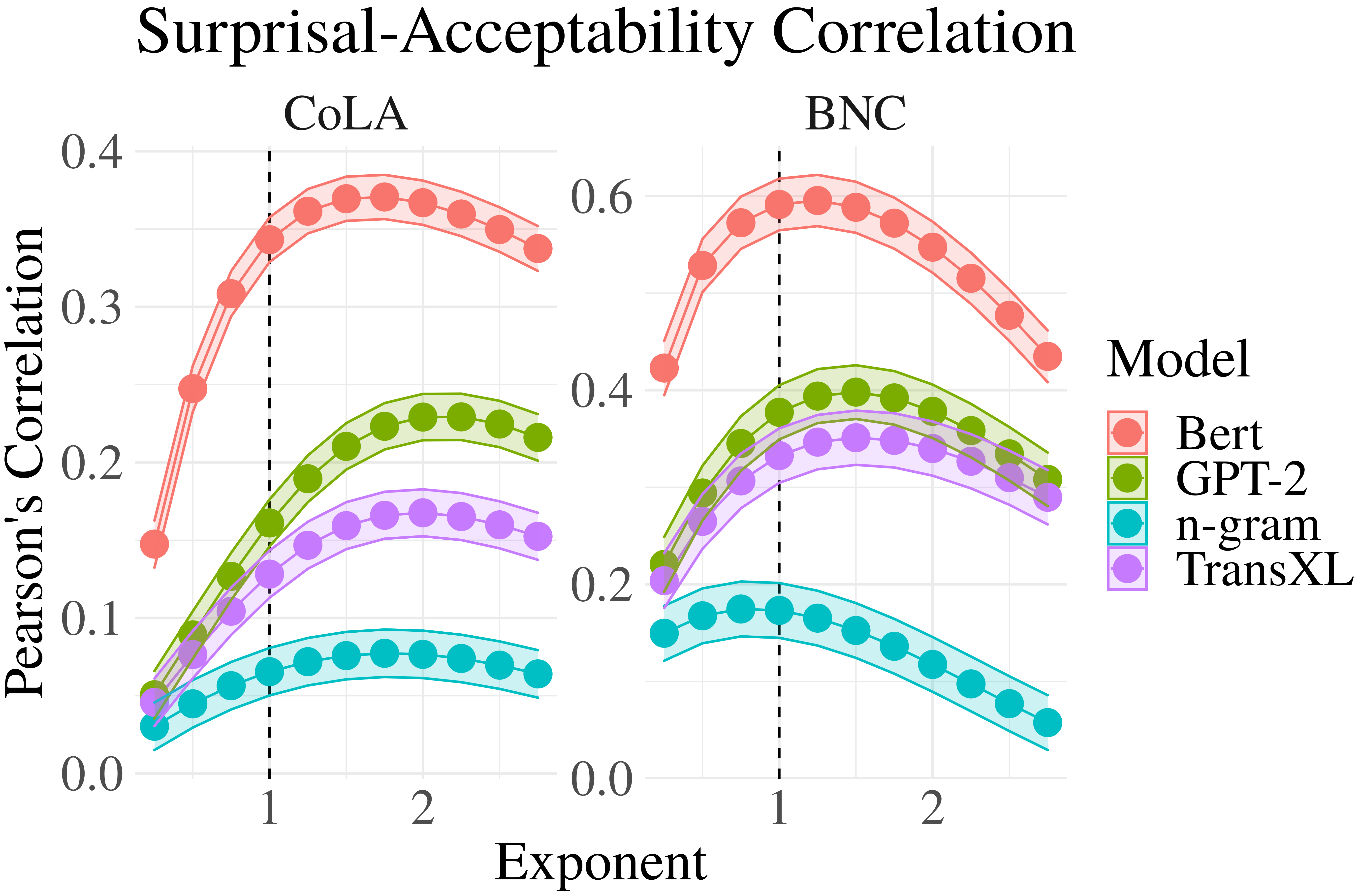
Figure 1: Correlation coefficient between (negative) sum of surprisals raised to the $k^{\text{th}}$ power and linguistic acceptability judgments of a sentence. The higher correlation when $k>1$ implies sentences with a more uniform distribution of information are more acceptable.

The uniform information density (UID) hypothesis (Fenk and Fenk, 1980; Levy and Jaeger, 2007) states that language users prefer when information content (measured information-theoretically as surprisal) is distributed as smoothly as possible throughout an utterance. The studies adduced in support of this hypothesis in language production span levels of linguistic structure: from phonetics Aylett and Turk (2004) to lexical choice Mahowald et al. (2013), to syntax Jaeger (2010), and to discourse (Torabi Asr and Demberg 2015) (though see Zhan and Levy 2018, 2019). Despite this evidence, there are several aspects of the UID hypothesis that lack clarity or unity. For example, there is a dearth of converging evidence from studies in language comprehension. Furthermore, multiple candidate operationalizations of UID have been proposed, each without formal justification for their choices Collins (2014); Jain et al. (2018); Meister et al. (2020); Wei et al. (2021).

In this work, we attempt to shed light on these issues: we first study the relationship between the distribution of information content throughout a sentence and native speakers' (i) sentence-level reading times and (ii) sentence acceptability judgments. While our results for sentence-level reading times do not contradict previous word-level reading time analyses (e.g., Smith and Levy 2013; Goodkind and Bicknell 2018a), which have shown a linear effect of surprisal, they suggest that a slight super-linear effect may likewise be a plausible explanation—which is in line with predictions of the UID hypothesis. For sentence acceptability judgments, we see more concrete signs of a super-linear effect of sentence-level surprisal (see Fig. 1), consistent with a preference for UID in language. Given these findings, we next ask how we can best measure UID. We review previous results supporting UID, in search of an operationalization and find that in most of these studies, adherence to UID is measured via an analysis of individual linguistic units, without direct consideration for the information content carried by surrounding units Frank and Jaeger (2008); Jaeger (2010); Mahowald et al. (2013). Such a definition fails to account for the distribution across the signal as a whole.

Consequently, we present and motivate a set of plausible operationalizations—either taken from the literature or newly proposed. Given our earlier results, we posit that good operationalizations of UID should provide strong explanatory power for human judgments of linguistic acceptability and potentially reading times. In this search, we additionally explore with respect to which linguistic unit—a phrase, sentence, document, or language as a whole—uniformity should be measured. Our results provide initial evidence that the best definition of UID may be a super-linear function of word surprisal. Further, we see that a regression towards the mean information content of the entire language, rather than a local information rate, may better capture the pressure for UID in natural language, a theory that falls in line with its information-theoretical interpretation, i.e., that language users maximize the use of a hypothetical noisy channel during communication.author=tiago,color=cyan!40,size=,fancyline,caption=,]Should we add a footnote here about our other paper in emnlp? Perhaps saying. "In x we investigate this same pressure cross-linguistically. Finding evidence for a regression towards a cross-linguistic mean information content."author=clara,color=orange,size=,fancyline,caption=,]If we have the space in the end

2 Processing Effort in Comprehension

In psycholinguistics, there are a number of theories that explain how the effort required to process language varies as a function of some perceived linguistic unit. Several of these are founded in information theory Shannon (1948), using the notion of language as a communication system in order to build computational models of processing. Under such a framework, linguistic units convey information, and the exact amount of information a unit carries can be quantified as its surprisal—also termed Shannon information content. Formally, let us consider a linguistic signal $\mathbf{u}=\langle u_{1},\dots,u_{N}\rangle$ as a sequence of linguistic units, e.g., words or morphemes; the standard definition of surprisal is then $s(u_{n})\mathrel{\stackrel{{\scriptstyle\textnormal{def}}}{{=}}}-\log p(u_{n}\mid\mathbf{u}_{<n})$, i.e., a unit's negative log-probability conditioned on its prior context. Note that under this definition, low probability items are seen as more informative, which reflects the intuition that unpredictable items convey more information than predictable ones. With this background in mind, we now review two prominent examples of information-theoretic models of language processing: surprisal theory and the uniform information density hypothesis.

2.1 Surprisal Theory

Surprisal theory Hale (2001) posits that the incremental load of processing a word is directly related to how unexpected the word is in its context, i.e., its surprisal. Mathematically formulated, the processing effort required for the word $u_{n}$ follows a linear relationship with respect to its surprisal:

$$\mathrm{Effort}(u_{n})\propto s(u_{n})$$ (1)

Over the years, surprisal theory has been further motivated and received wide empirical support Levy (2008); Brouwer et al. (2010). Notably, a number of works give evidence that this relationship (between processing effort and surprisal) is indeed linear (equivalently, logarithmic in probability; Smith and Levy 2013; Frank et al. 2013; Goodkind and Bicknell 2018b, though see Brothers and Kuperberg 2021).

2.2 Uniform Information Density

Given the formal definition of surprisal, the information content of the entire linguistic signal $\mathbf{u}$ can be quantified as the sum of individual surprisals. Following Eq. 1, the effort to process $\mathbf{u}$ would thus be proportional to this sum, i.e.:

$$\mathrm{Effort}(\mathbf{u})\propto\sum_{n=1}^{N}s(u_{n})$$ (2)

But this has a counter-intuitive consequence. Suppose a speaker has a fixed number of bits of information to convey. Eq. 2 predicts that all ways of distributing that information in an utterance would involve equal processing effort: packing it all into a single, short utterance; spreading it out thinly in an extremely long utterance; dispersing it in a highly uneven profile throughout an utterance.

The theory of uniform information density (UID; Fenk and Fenk 1980; Genzel and Charniak 2002; Bell et al. 2003; Aylett and Turk 2004; Levy and Jaeger 2007) attempts to reconcile the role of surprisal in determining processing effort with the intuition that perhaps not all ways of distributing information content have equal effect on overall processing effort. Rather, UID predicts that communicative efficiency is maximized when information—again quantified as per-unit surprisal—is distributed as uniformly as possible throughout a signal. One way of deriving this prediction is to hypothesize that the processing effort for a sentence is an additive function of (i) a super-linear function of surprisal; and (ii) utterance length:

$$\mathrm{Effort}(\mathbf{u})\propto\sum_{n=1}^{N}s(u_{n})^{k}+c\cdot N$$ (3)

for some constant $c>0$ and $k>1$. The above equation implies that high surprisal instances require disproportionately high processing effort from the language user. Rather, a uniform distribution of $s(u_{n})$—which for fixed $N$ and total information is the unique minimizer of Eq. 3—would incur the least processing effort. Proof given in App. A.

Due to its support by a number of studies, the UID hypothesis has received considerable recognition in the cognitive science community. Such verifications, though, derive mostly from the tendencies implied by Eq. 3—as opposed to its direct verification. Take the original Levy and Jaeger (2007) as an example: while they propose a formal operationalization of UID, they evaluate their hypothesis by analyzing a surprisal vs. sentence length trade-off rather than assessing the operationalization directly. Furthermore, most UID studies investigate individual word surprisals, without regard for their distribution within the sequence (Aylett and Turk, 2004; Mahowald et al., 2013, inter alia).

3 Quantifying Linguistic Uniformity

UID is, by its definition, a smoothing effect; it can be seen as a regression to a mean information rate—either measured as the surprisal per lexical unit (in written text, as we analyze here), or surprisal per time unit (in speech data). However, there are multiple ways the hypothesis may be interpreted. As a concrete example, we turn to Collins's (2014) fourth figure, which we recreate here in Fig. 2. In its perhaps better-known form, UID suggests that language transmission should happen at a roughly constant rate, close to the channel capacity, i.e., there is a fixed (and perhaps cross-linguistic; Coupé et al. 2019; Pimentel et al. 2021) value from which a unit's information density should never heavily deviate. Under this interpretation, S1 (red) adheres more closely to UID, as information content per word varies less—in absolute terms—across the sentence. We can formalize this notion of UID using an inverse relationship to some per-unit distance metric $\Delta(\cdot,\cdot)$ as follows:

$$\textsc{uid}^{-1}(\mathbf{u})=\frac{1}{N}\sum_{n=1}^{N}\Delta(s(u_{n}),\mu_{c})$$ (4)

where $\mu_{c}$ is a target (mean) information rate—presumably at a theoretical channel's capacity. This mathematical relationship reflects the intuition that the further the units in a linguistic signal are from the average information rate $\mu_{c}$, the less the signal adheres to UID.

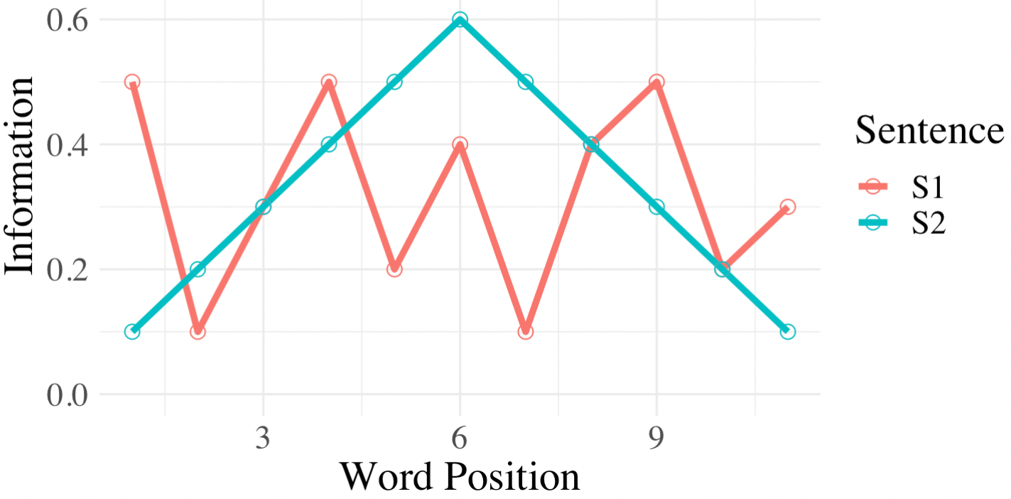
Figure 2: Information distribution across words of two hypothetical sentences. Recreation of Fig. 4 in Collins's (2014).

We may, however, also interpret UID as a pressure to avoid rapidly shifting from information dense (and therefore cognitively taxing) sections to sections requiring minimal processing effort. Rather, in an optimal setting, there should be a smooth transition between information sparse and dense components of a signal. Under this interpretation, we might believe S2 (blue) to adhere more closely to UID, as local changes are gradual. We can formalize this version of UID as

$$\textsc{uid}^{-1}(\mathbf{u})=\frac{1}{N-1}\sum_{n=2}^{N}\Delta(s(u_{n}),s(u_{n-1}))$$ (5)

The difference between these two is concisely summarized as minimizing global vs. local variability. The former definition has arguably received more attention; studies such as Frank and Jaeger (2008), among others, analyze UID through regression towards a global mean. Yet, there are arguments that variability should instead be measured locally Collins (2014); Bloem (2016).

3.1 Regressing to Which Mean?

Notably, there is an aspect of the global variability presented in Eq. 4 that remains underspecified: what exactly is $\mu_{c}$? A mean information rate may be with respect to a phrase, a sentence or even a language as a whole; this rate could even span across languages, a definition that nicely aligns with recent cross-linguistic experiments on spoken language data that argue for a universal channel capacity Pellegrino et al. (2011); Coupé et al. (2019). Yet, the former definitions likewise seem plausible.

To motivate this argument, consider the relationship between cadence in literary writing and UID. We loosely define cadence as the rhythm and speed of a piece of text, which should have a close relationship to the dispersion of information. When writing prose, authors typically vary cadence across sentences, interspersing short, impactful (i.e., high information) sentences within series of longer sentences to avoid repetitiveness. We have done so here, in this paper. Yet, intuitively, this practice does not lead to particularly high processing costs, at least for a native speaker. Indeed, some would argue that such fluctuations make text easier to read. This example motivates a pull towards a more context-dependent—perhaps sentence-level—rather than language-level mean information rate.

While a number of findings undoubtedly demonstrate a pressure against high (and sometimes even inordinately low) surprisal—which aligns with the first (global) interpretation of the UID hypothesis—their experimental setups, in general, do not provide evidence for or against a more local interpretation, such as the one just described. We now define a number of UID operationalizations that encompass these different interpretations, subsequently analyzing them in § 4.3.

3.2 Operationalizing UID

The first operationalization on which we will focus follows from Eq. 3, suggesting a super-linear effect of surprisal on processing effort:

$$\textsc{uid}^{-1}(\mathbf{u})=\frac{1}{N}\sum_{n=1}^{N}s(u_{t})^{k}\quad\quad{\color[rgb]{.5,.5,.5}(k>1)}$$ (6)

where $k$ controls the strength of super-linearity.

A second operationalization, similar to Eq. 4, implies a pressure for mean regression:

$$\textsc{uid}^{-1}(\mathbf{u})=\frac{1}{N}\sum_{n=1}^{N}(s(u_{n})-\mu)^{2}$$ (7)

Note that we may take $\mu$ from a number of different contexts. For example, $\mu_{\mathrm{sent}}=\frac{1}{N}\sum_{n=1}^{N}s(u_{n})$ for sentence $\langle u_{1},\dots,u_{N}\rangle$ implies a sentence-level mean regression, whereas average surprisal over an entire language $\mu_{\mathrm{lang}}$ suggests a regression to a (perhaps language-specific) channel capacity. Both definitions more closely align with our global interpretation of UID, i.e., that S1 (red) of Fig. 2 may exhibit a more ``uniform'' distribution of information.

Similarly, we can compute the local variance in a sentence as

$$\textsc{uid}^{-1}(\mathbf{u})=\frac{1}{N-1}\sum_{n=2}^{N}(s(u_{n})-s(u_{n-1}))^{2}$$ (8)

which, in contrast to Eq. 6, aligns more with our local interpretation of UID.

We may also interpret UID as a pressure to minimize a signal's maximum per-unit surprisal, as this may be a point of inordinately high cognitive load for the comprehender:

$$\textsc{uid}^{-1}(\mathbf{u})=\overset{N}{\max_{n=1}}\,s(u_{n})$$ (9)

For completeness, we further propose another potential measure of UID compliance inspired by the information-theoretic nature of UID. We consider the Rényi entropy (Rényi, 1961) of a probability distribution $p$, defined as:

$$\mathrm{H}_{k}(p)=\frac{1}{1-k}\log\sum_{x\in\mathcal{X}}p(x)^{k}$$ (10)

where $\mathcal{X}$ is the support of the distribution $p$. Notably, the Rényi entropy, which is maximized when $p$ is uniform, becomes the Shannon entropy in the limit as $k\rightarrow 1$. However, for $k>1$, high probability items contribute disproportionately to this sum, which in our context, would translate to an emphasis on low-surprisal items. Thus, we do not expect it to be a good operationalization of (inverse) UID. However, the opposite holds for $k<1$, where Rényi entropy can be seen as producing an extra cost for low-probability, i.e., high-surprisal items. Thus, in terms of UID, we take:

$$\textsc{uid}^{-1}(\mathbf{u})=\begin{cases}\mathrm{H}_{k}(\widehat{p})&\textbf{if}\,\,\,k<1\\ \mathrm{H}_{k}^{-1}(\widehat{p})&\textbf{otherwise}\end{cases}$$ (11)

where $\widehat{p}$ is a distribution over $u_{1},\dots,u_{N}$ normalized to sum to 1.

3.3 UID, Effort and Acceptability

We now revisit the processing effort of a sentence, rewriting it in terms of our UID operationalizations

$$\mathrm{Effort}(\mathbf{u})\propto\textsc{uid}^{-1}(\mathbf{u})\cdot N+c\cdot N$$ (12)

i.e., processing effort is proportional to the interaction between (i.e., multiplication by) $\textsc{uid}^{-1}$ and sentence length. Note that when using our operationalization of UID from Eq. 6, this equation reverts to Levy's (2005) original Eq. 3. Further, this equation with $k=1$ and $c=0$ recovers the hypothesis under surprisal theory. Following previous work (Frank and Bod, 2011; Goodkind and Bicknell, 2018a, inter alia), we then model reading time as $\mathrm{ReadingTime}(\mathbf{u})\propto\mathrm{Effort}(\mathbf{u})$; in words, (proportionally) more time is taken to read more cognitively demanding sentences.

We further consider the relationship between UID and linguistic acceptability; we posit that

$$\mathrm{Acceptability}^{-1}(\mathbf{u})\propto\textsc{uid}^{-1}(\mathbf{u})\cdot N$$ (13)

i.e., the linguistic acceptability of a sentence has an inverse relationship with processing effort (withholding the additional penalty for length). Intuitively, sentences that are easier to process are more probably acceptable sentences, and vice versa. While not comprehensive, there is evidence that this simple model (at least to some extent) captures the relationship between these two variables Topolinski and Strack (2009). Given these models, we now evaluate our different operationalizations based on their predictive power of psychometric variables.

4 Experiments

Data.

We employ reading time data in English from 4 corpora over 2 modalities: the Natural Stories Futrell et al. (2018) and Brown Smith and Levy (2013) Corpora, which contain self-paced reading time data, as well as the Provo Luke and Christianson (2018) and Dundee Corpora Kennedy et al. (2003), which contain eye movements during reading. For acceptability judgments, also in English, we use the Corpus of Linguistic Acceptability (CoLA; Warstadt et al. 2019) and the bnc dataset Lau et al. (2017). Notably, Natural Stories and CoLA by design contain wide coverage of syntactic and semantic phenomena. We provide further details of each of these datasets, including pre-processing, statistics and data-gathering processes, in App. B.

4.1 Estimating Surprisal

Since we do not have access to the ground-truth values of conditional probabilities of observing linguistic units given their context (i.e., surprisals), we must instead estimate these probabilities. This is typical practice in psycholinguistic studies Demberg and Keller (2008); Mitchell et al. (2010); Fernandez Monsalve et al. (2012). For example, Hale (2001) uses a probabilistic context-free grammar; Smith and Levy (2013) use $n$-gram language models.author=clara,color=orange,size=,fancyline,caption=,]would have been interesting to test this stuff out with parse steps, like with a PCFG

In general, the psychometric predictive power of surprisal estimates from a model correlates highly with model quality (Frank and Bod, 2011; Fossum and Levy, 2012; Goodkind and Bicknell, 2018a, as traditionally measured by perplexity;). Further, Transformer-based models appear to have superior psychometric predictive power in comparison to other architectures Wilcox et al. (2020). We employ GPT-2 Radford et al. (2019), TransformerXL Dai et al. (2019), and BERT Devlin et al. (2019)—state-of-the-art language models. We additionally include results using a 5-gram model, estimated using Modified Kneser–Essen–Ney Smoothing Ney et al. (1994), to allow for an easier comparison with results from earlier works exploring UID in reading time data. All probability estimates are computed at the word-level. Further details are given in App. B.

4.2 Assessing Predictive Power

In our experiments, we analyze the ability of different functions of surprisal to predict psychometric data, namely the total time spent reading sentences in self-paced reading and eye tracking studies (see App. B)—and perceived linguistic acceptability, in order to better understand the relationship of surprisal with language processing. For reading times, we use the sum across word-level times as our sentence-level metric. Notably for eye movement datasets, our analysis of sentence-level reading times is novel: previous work has generally focused on how long readers spend on a word before progressing beyond it (often called the ``first pass;'' Rayner (1998)), but sentence-level measures include time re-reading content after having progressed beyond it. Linguistic acceptability data are available and assessed only at the sentence-level.

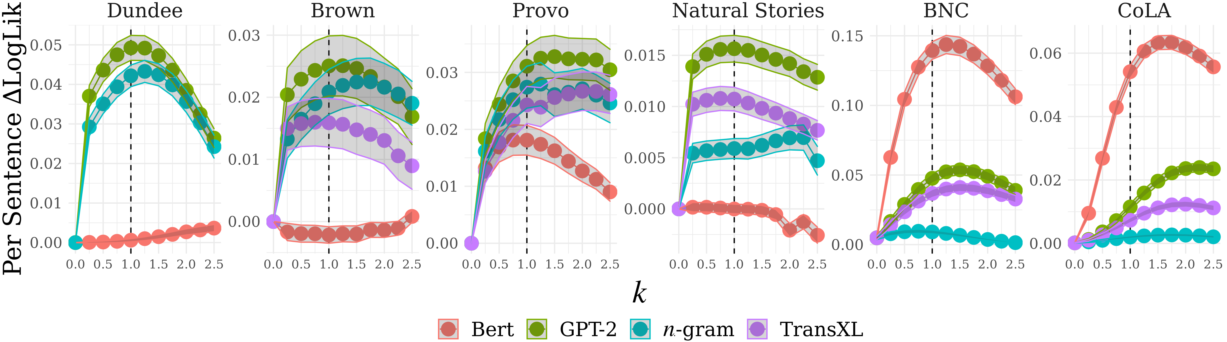
Figure 3: Mean $\Delta\mathrm{LogLik}$ as a function of the exponent $k$ for the sentence-level predictor (Eq. 3) of reading time and linguistic acceptability. Shaded region connects standard error estimates from each point. We observe that often, our predictor with $k>1$ explains the data at least as well as $k=1$. Baseline models against which $\Delta\mathrm{LogLik}$ is computed are specified in § 4.2. For reading times, the augmented models additionally contain fixed effects and per-subject random effects slopes for the UID operationalization; for acceptability judgments, only a fixed effect for the UID operationalization is added.

As we are interested in the relationship between UID and both reading times and acceptability judgments—in particular, the relationships described by Eqs. 12 and 13—we turn to linear regression models. For reading time data, as our baseline models, we specifically use linear mixed-effects models, with random effect terms (slopes for total word count at the sentence-level and intercepts at the word-level) for each subject to control for individual reading behaviors. We additionally control for other variables known to influence reading time: at the sentence-level, our fixed effects include total word count and number of words with recorded fixations (per subject and sentence); results including fixed effects for sums of both individual word character lengths and word unigram log-probabilities (as estimated from WikiText 103; Merity et al. 2017) are given in App. C. At the word-level (only our last set of experiments), our fixed effects include linear terms for word log-probability, unigram log-probability, and character length, and the interaction of the latter two. We additionally include the same predictors from the previous word, a common practice due to known spillover effects observed in both types of measurement. These are standard predictors in reading time analyses Smith and Levy (2013); Goodkind and Bicknell (2018b); Wilcox et al. (2020). For linguistic acceptability data, we use logistic regression models with solely an intercept term as our baseline predictor; results when including summed unigram log-probability or sentence length as predictors yielded similar trends (see App. C).

We evaluate each model relative to a baseline, containing only the control features just mentioned. Specifically, performance assessments are computed between models that differ by solely a single predictor; for reading time data, we include both a fixed and (per-subject) random slope for this predictor. Following Wilcox et al. (2020), we report $\Delta\mathrm{LogLik}$: the mean difference in log-likelihood of the response variable between the two models. A positive $\Delta\mathrm{LogLik}$ value indicates that a given data point is more probable under the comparison model, i.e., it more closely fits the observed data. To avoid overfitting, we compute $\Delta\mathrm{LogLik}$ solely on held-out test data, averaged over 10-fold cross validation. See App. B for evaluation details.

4.3 Results

Evidence of UID in Reading Times and Acceptability Judgments.

We first assess the ability of our processing cost model (Eq. 3) to predict reading times. In a similar fashion, we use Eq. 13 with Eq. 6 to predict acceptability scores. Recall from § 2 that if the true relationship between surprisal and sequence-level processing effort is expressed by Eq. 3 with $k>1$, then there must exist a pressure towards uniform information density. Thus, if we observe that a linear model using $\sum_{n=1}^{N}s(u_{n})^{k}$ as a predictor explains the observed data better when $k>1$, it suggests a preference for the uniform distribution of information in text. We report results for multiple corpora in Fig. 3.

We see that in general, the best fit to the data is achieved not when our cost equations use $k=1$, but rather a slightly larger value of $k$ (see also Tab. 1). Notably for reading time data, a conclusion that $k>1$ is optimal contradicts a number of prior works that have judged the relationship between surprisal and reading time to be linear. We discuss this point further in § 5. Yet for the reading time datasets, the $k=1$ predictor is typically still within the standard error of the best predictor, meaning that the linear hypothesis is not ruled out. For acceptability data, we see more distinctly that $k>1$ leads to the best predictor, especially when using true surprisal estimates (i.e., models aside from BERT). This result suggests that a more uniform distribution of information more strongly correlates with linguistic acceptability (see also Fig. 1 for explicit correlation analysis).

We perform hypothesis tests to formally test whether our models of processing cost and linguistic acceptability have higher predictive power—as measured by $\Delta\mathrm{LogLik}$—when using a super-linear vs. linear function of surprisal. Specifically, we take our null hypothesis to be that $k=1$ provides better or equivalent predictive power to $k>1$. We use a paired t-tests, where we aggregate sentence-level data across subjects for reading time datasets so as not violate independence assumptions. We use a Bonferroni correction to account for the consideration of multiple models with $k>1$. We find that we consistently reject the null hypothesis at significance level $\alpha=0.001$ for acceptability data experiments (aside from under the $n$-gram model). For reading time data, we never reject the null hypothesis, again confirming that the linear hypothesis may hold true in this setting.

Another important observation is that the pseudo log-probability estimates from a cloze language model (BERT) work remarkably well when used to predict acceptability judgments, yet remarkably poorly for reading time estimates. We also see a less super-linear effect (higher predictive power for $k\approx 1$) of surprisal in sentence acceptability for cloze than for auto-regressive models.

Predictor Reading Time Acceptability Dundee Brown Provo NS CoLA bnc $\mathrm{Super}\text{-}\mathrm{Linear}$ ($k=0.25$) $3.70{\color[rgb]{0.0,0.0,0.5}\bf\scriptstyle\,(\pm 0.27)}$ $1.88{\color[rgb]{0.0,0.0,0.5}\bf\scriptstyle\,(\pm 0.44)}$ $1.73{\color[rgb]{0.0,0.0,0.5}\bf\scriptstyle\,(\pm 0.27)}$ $1.40{\color[rgb]{0.0,0.0,0.5}\bf\scriptstyle\,(\pm 0.12)}$ $0.90{\color[rgb]{0.0,0.0,0.5}\bf\scriptstyle\,(\pm 0.03)}$ $6.11{\color[rgb]{0.0,0.0,0.5}\bf\scriptstyle\,(\pm 0.13)}$ $\mathrm{Super}\text{-}\mathrm{Linear}$ ($k=1$) $\bf{4.93}{\color[rgb]{0.0,0.0,0.5}\bf\scriptstyle\,(\pm 0.32)}$ $2.38{\color[rgb]{0.0,0.0,0.5}\bf\scriptstyle\,(\pm 0.48)}$ $3.07{\color[rgb]{0.0,0.0,0.5}\bf\scriptstyle\,(\pm 0.36)}$ $\bf{1.58}{\color[rgb]{0.0,0.0,0.5}\bf\scriptstyle\,(\pm 0.13)}$ $5.28{\color[rgb]{0.0,0.0,0.5}\bf\scriptstyle\,(\pm 0.07)}$ $13.89{\color[rgb]{0.0,0.0,0.5}\bf\scriptstyle\,(\pm 0.19)}$ $\mathrm{Super}\text{-}\mathrm{Linear}$ ($k=1.25$) $\bf{4.93}{\color[rgb]{0.0,0.0,0.5}\bf\scriptstyle\,(\pm 0.31)}$ $\bf{2.39}{\color[rgb]{0.0,0.0,0.5}\bf\scriptstyle\,(\pm 0.49)}$ $3.24{\color[rgb]{0.0,0.0,0.5}\bf\scriptstyle\,(\pm 0.37)}$ $1.55{\color[rgb]{0.0,0.0,0.5}\bf\scriptstyle\,(\pm 0.13)}$ $5.92{\color[rgb]{0.0,0.0,0.5}\bf\scriptstyle\,(\pm 0.07)}$ $\bf{14.35}{\color[rgb]{0.0,0.0,0.5}\bf\scriptstyle\,(\pm 0.19)}$ $\mathrm{Super}\text{-}\mathrm{Linear}$ ($k=1.5$) $4.74{\color[rgb]{0.0,0.0,0.5}\bf\scriptstyle\,(\pm 0.31)}$ $2.34{\color[rgb]{0.0,0.0,0.5}\bf\scriptstyle\,(\pm 0.49)}$ $\bf{3.25}{\color[rgb]{0.0,0.0,0.5}\bf\scriptstyle\,(\pm 0.37)}$ $1.50{\color[rgb]{0.0,0.0,0.5}\bf\scriptstyle\,(\pm 0.13)}$ $\bf{6.18}{\color[rgb]{0.0,0.0,0.5}\bf\scriptstyle\,(\pm 0.07)}$ $14.22{\color[rgb]{0.0,0.0,0.5}\bf\scriptstyle\,(\pm 0.19)}$ $\mathrm{Super}\text{-}\mathrm{Linear}$ ($k=2$) $3.85{\color[rgb]{0.0,0.0,0.5}\bf\scriptstyle\,(\pm 0.28)}$ $2.11{\color[rgb]{0.0,0.0,0.5}\bf\scriptstyle\,(\pm 0.47)}$ $3.22{\color[rgb]{0.0,0.0,0.5}\bf\scriptstyle\,(\pm 0.36)}$ $1.40{\color[rgb]{0.0,0.0,0.5}\bf\scriptstyle\,(\pm 0.13)}$ $6.04{\color[rgb]{0.0,0.0,0.5}\bf\scriptstyle\,(\pm 0.07)}$ $12.75{\color[rgb]{0.0,0.0,0.5}\bf\scriptstyle\,(\pm 0.18)}$ $\mathrm{Variance}$ (lang) $2.37{\color[rgb]{0.0,0.0,0.5}\bf\scriptstyle\,(\pm 0.22)}$ $1.37{\color[rgb]{0.0,0.0,0.5}\bf\scriptstyle\,(\pm 0.39)}$ $2.46{\color[rgb]{0.0,0.0,0.5}\bf\scriptstyle\,(\pm 0.33)}$ $0.73{\color[rgb]{0.0,0.0,0.5}\bf\scriptstyle\,(\pm 0.10)}$ $5.64{\color[rgb]{0.0,0.0,0.5}\bf\scriptstyle\,(\pm 0.07)}$ $11.26{\color[rgb]{0.0,0.0,0.5}\bf\scriptstyle\,(\pm 0.17)}$ $\mathrm{Variance}$ (sent) $2.01{\color[rgb]{0.0,0.0,0.5}\bf\scriptstyle\,(\pm 0.20)}$ $1.16{\color[rgb]{0.0,0.0,0.5}\bf\scriptstyle\,(\pm 0.35)}$ $2.59{\color[rgb]{0.0,0.0,0.5}\bf\scriptstyle\,(\pm 0.34)}$ $0.80{\color[rgb]{0.0,0.0,0.5}\bf\scriptstyle\,(\pm 0.11)}$ $1.86{\color[rgb]{0.0,0.0,0.5}\bf\scriptstyle\,(\pm 0.04)}$ $7.56{\color[rgb]{0.0,0.0,0.5}\bf\scriptstyle\,(\pm 0.14)}$ $\mathrm{LocalVariance}$ $1.93{\color[rgb]{0.0,0.0,0.5}\bf\scriptstyle\,(\pm 0.20)}$ $1.08{\color[rgb]{0.0,0.0,0.5}\bf\scriptstyle\,(\pm 0.36)}$ $2.15{\color[rgb]{0.0,0.0,0.5}\bf\scriptstyle\,(\pm 0.30)}$ $0.64{\color[rgb]{0.0,0.0,0.5}\bf\scriptstyle\,(\pm 0.09)}$ $1.44{\color[rgb]{0.0,0.0,0.5}\bf\scriptstyle\,(\pm 0.04)}$ $4.88{\color[rgb]{0.0,0.0,0.5}\bf\scriptstyle\,(\pm 0.12)}$ $\mathrm{Max}$ $1.74{\color[rgb]{0.0,0.0,0.5}\bf\scriptstyle\,(\pm 0.20)}$ $1.11{\color[rgb]{0.0,0.0,0.5}\bf\scriptstyle\,(\pm 0.39)}$ $1.17{\color[rgb]{0.0,0.0,0.5}\bf\scriptstyle\,(\pm 0.27)}$ $0.68{\color[rgb]{0.0,0.0,0.5}\bf\scriptstyle\,(\pm 0.12)}$ $1.16{\color[rgb]{0.0,0.0,0.5}\bf\scriptstyle\,(\pm 0.03)}$ $5.00{\color[rgb]{0.0,0.0,0.5}\bf\scriptstyle\,(\pm 0.12)}$ $\mathrm{Entropy}$ ($k=0.25$) $1.16{\color[rgb]{0.0,0.0,0.5}\bf\scriptstyle\,(\pm 0.16)}$ $0.30{\color[rgb]{0.0,0.0,0.5}\bf\scriptstyle\,(\pm 0.24)}$ $1.35{\color[rgb]{0.0,0.0,0.5}\bf\scriptstyle\,(\pm 0.22)}$ $0.25{\color[rgb]{0.0,0.0,0.5}\bf\scriptstyle\,(\pm 0.13)}$ $0.02{\color[rgb]{0.0,0.0,0.5}\bf\scriptstyle\,(\pm 0)}$ $0.03{\color[rgb]{0.0,0.0,0.5}\bf\scriptstyle\,(\pm 0.01)}$ $\mathrm{Entropy}$ ($k=1$) Shannon $-0.01{\color[rgb]{0.0,0.0,0.5}\bf\scriptstyle\,(\pm 0.01)}$ $0{\color[rgb]{0.0,0.0,0.5}\bf\scriptstyle\,(\pm 0)}$ $0.01{\color[rgb]{0.0,0.0,0.5}\bf\scriptstyle\,(\pm 0)}$ $0{\color[rgb]{0.0,0.0,0.5}\bf\scriptstyle\,(\pm 0)}$ $0{\color[rgb]{0.0,0.0,0.5}\bf\scriptstyle\,(\pm 0)}$ $7.90{\color[rgb]{0.0,0.0,0.5}\bf\scriptstyle\,(\pm 0.14)}$ $\mathrm{Entropy}$ ($k=2$) Renyi $-0.01{\color[rgb]{0.0,0.0,0.5}\bf\scriptstyle\,(\pm 0)}$ $0{\color[rgb]{0.0,0.0,0.5}\bf\scriptstyle\,(\pm 0.01)}$ $0{\color[rgb]{0.0,0.0,0.5}\bf\scriptstyle\,(\pm 0.01)}$ $0{\color[rgb]{0.0,0.0,0.5}\bf\scriptstyle\,(\pm 0)}$ $0{\color[rgb]{0.0,0.0,0.5}\bf\scriptstyle\,(\pm 0)}$ $8.38{\color[rgb]{0.0,0.0,0.5}\bf\scriptstyle\,(\pm 0.14)}$

Table 1: $\Delta\mathrm{LogLik}$ in $10\text{e-}2$ nats when adding different UID operationalizations as predictors of reading time and linguistic acceptability. Surprisal estimates from GPT-2 are used. We use the same paradigm for baseline and augmented models as in Fig. 3. Other setups show similar trends (App. C).

author=roger,color=green!40,size=,fancyline,caption=,]This table and Figure 3 still don't look totally aligned, eg Provo is optimal at k=2 in the table but in the figure it looks like it's k=1.75?author=clara,color=orange,size=,fancyline,caption=,]yes, but k=1.75 isn't included in the table :/ I skipped it for space. Do you think I should add it in?

Evaluating Operationalizations of UID.

We next ask: what are appropriate measures of UID in a linguistic signal? In an effort to answer this question, we explore the predictive power of the different operationalizations of UID proposed in § 3 for our psycholinguistic data; given our evidence of UID in the prior section, we posit that better operationalizations should likewise provide stronger explanatory power than poor ones. We again fit linear models using Eqs. 12 and 13, albeit with each analyzed UID operationalization as our predictor. We use surprisal estimates from GPT-2, as it was consistently the autoregressive language model with the best predictive power.

Results in Tab. 1 show that, in general, the family of $\mathrm{Super}\text{-}\mathrm{Linear}$ (Eq. 6) operationalizations (for $k\geq 1$) and a language-wide notion of $\mathrm{Variance}$ (Eq. 7) provide the largest increase in explanatory power relative to the baseline models, suggesting they may be the best quantifications of UID. While the $\mathrm{Max}$ (Eq. 9) and $\mathrm{Variance}$ (Eq. 7) predictors also provide good explanatory power, they are consistently lower across datasets. Further, language-level $\mathrm{Variance}$ seems to produce stronger predictors for psychometric data than sentence-level and $\mathrm{Local\,Variance}$—an observation driving our next set of experiments. Notably, the $\mathrm{Entropy}$ predictors do quite poorly in comparison to other operationalizations, especially for $k\geq 1$. These results suggest that a sentence-level notion of entropy may not capture the UID phenomenon well, which is perhaps surprising, given that it is a natural measure of the uniformity of information.

Exploring the Scope of UID's Pressure.

author=roger,color=green!40,size=,fancyline,caption=,]Isn't this paragraph now outdated/superseded given the new Table 1 results? Should we just ditch it?author=clara,color=orange,size=,fancyline,caption=,]I don't think its outdated, actually. The results in Table 1 are not too different than they were before. Variance was never the best operationalization but its the operationalization that gives us the chance to ask this question Each of our operationalizations in § 3 are computed at the sequence-level. Thus, it is natural to ask, what should be the scope of a sequence when considering information uniformity? In an effort to answer this question, we explore how the predictive power of our UID operationalizations change as we vary the window sizes over which they are computed. Specifically, we will look at ability to predict per-word reading times; we make use of the $\mathrm{Variance}$ operationalization as our predictor (which demonstrated good performance in our sentence-level experiments) albeit with a word-level version:

$$\textsc{uid}^{-1}(u_{n})=(s(u_{n})-\mu)^{2}$$ (14)

where $\mu$ is mean surprisal computed across the previous $1,2,3,4$ or $n$ words or across the sentence, document, or language as a whole (as with unigram probabilities, $\mu_{\mathrm{lang}}$ is computed per model over WikiText 103). Tab. 1 and Fig. 4 show evidence that the pressure for uniformity may in fact be at a more global scale. Under each corpus, the higher-level predictors of UID appear to provide better explanatory power of reading times than more local predictors.

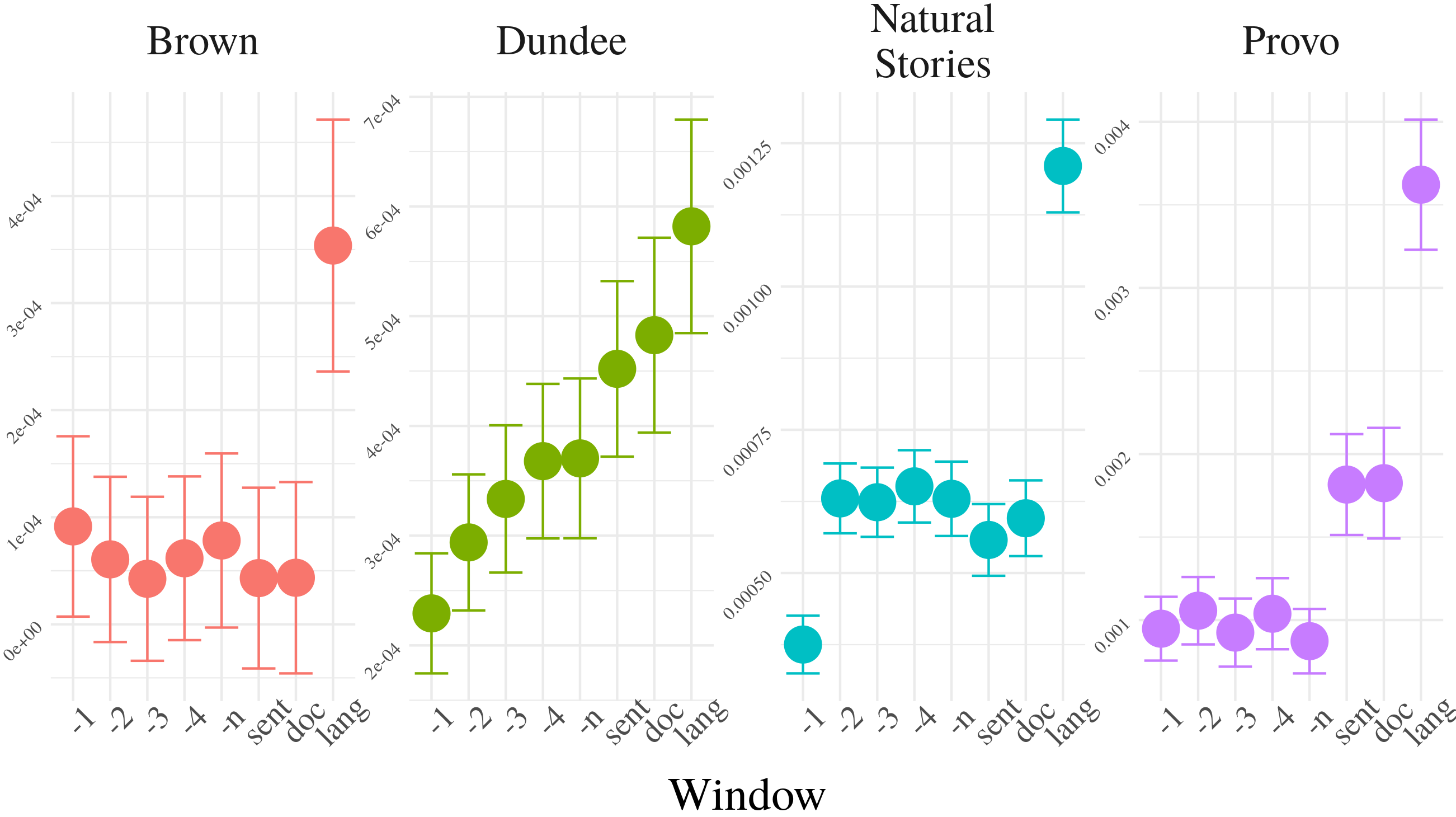
Figure 4: Per-token $\Delta\mathrm{LogLik}$ when changing the scope over which UID variance is computed (see Eq. 14). Surprisal estimates from GPT-2 are used. Baseline predictors are specified in § 4.2

5 Discussion

Most previous works investigating UID have looked for its presence in language production (Bell et al., 2003; Aylett and Turk, 2004; Levy and Jaeger, 2007; Mahowald et al., 2013, inter alia), while comprehension has received little attention. Collins (2014) and Sikos et al. (2017) are perhaps the only other works to find results in support of UID in this setting. Our findings are complementary to theirs; we take different analytical approaches but both observe a preference for the uniform distribution of information in a linguistic signal, although a similar analysis should be performed in the spoken domain before stronger conclusions can be drawn.

While our reading time results do not refute previous work showing linear effects of surprisal on word-level reading times Smith and Levy (2013); Goodkind and Bicknell (2018b); Wilcox et al. (2020), we see some suggestions that a super-linear hypothesis is also plausible, especially in the Provo corpus. Notably, most of these works did not test a parametric space of non-linear functional forms, instead confirming using visual inspection of the results of nonparametric fits. One exception, Smith and Levy (2013), explored the effects of adding a quadratic term for surprisal as a predictor of per-word reading times. Yet, if the true $k$ that describes the reading times–surprisal relationship were only slightly greater than 1, as our results suggest, this quadratic test might be too restrictive. Our approach, which explores a more fine-grained range of $k$, is potentially more comprehensive, and indeed we find that values of $k$ slightly greater than $1$ often fit the data at least as well as $k=1$, and can certainly not be ruled out. Other potential virtues of our analysis are (1) Our analysis is performed at the sentence- (rather than word-) level. This is arguably a better method for analyzing a sequence-level phenomenon, i.e., UID, and (2) specifically for eye movement data, we include re-reading times after the first pass.

Limitations and Future Directions.

A major limitation of this work is that the experimental analysis is limited to English (and Dutch, in the Appendix); while the pressure for uniformity—since explained by a cognitive process—should hold across languages, further experiments should be performed to verify these findings, especially since the relationship between model quality and psychometric predictive power has recently been called into question Kuribayashi et al. (2021). As such, while we find convincing preliminary evidence in our analyzed languages, we are not able to fully test the hypothesis that the pressure for UID is at the language-level. Further, we have no evidence as to whether there may be pressure towards a cross-linguistic $\mu_{c}$, which would be relevant to cross-linguistic interpretations of UID Pimentel et al. (2021).

Another important limitation of this work is the restriction to psychometric data from the written domain. To fully grasp the effects of the distribution of information in linguistic signals on language comprehension, spoken language data should be similarly analyzed. Of course, different factors are likely at play in language comprehension in the spoken domain, including e.g., the cognitive load of the speaker Pijpops et al. (2018); such factors may make it even more difficult to disentangle the contribution of different effects to comprehension. We leave this analysis for future work.

6 Conclusion

In this work, we revisit the UID hypothesis, providing both a quantitative and qualitative assessment of its various interpretations. We find suggestions that the UID formulation proposed in Levy (2005) may better predict processing effort in language comprehension than alternative formulations since proposed. We additionally find that a similar model explains linguistic acceptability judgments well, confirming a preference for UID in written language. We subsequently evaluate different operationalizations of UID, observing that a super-linear function of surprisal best explains psychometric data. Further, operationalizations associated with global interpretations of UID appear to provide better explanatory power than those of local interpretations, suggesting that perhaps the most accurate interpretation of UID should be the regression towards the mean information rate of a language.

Appendix A Theory

We use the standard definition of surprisal $s(u_{n})\mathrel{\stackrel{{\scriptstyle\textnormal{def}}}{{=}}}-\log p(u_{n}\mid\mathbf{u}_{<n})$, and define $s(\mathbf{u})=\sum_{n=1}^{N}s(u_{n})$ as the total surprisal of the entire signal $\mathbf{u}$.

Theorem A.1.

Assume a fixed $k>1$ and $c>0$, and assume $N\geq 1$. Then,

1. The objective $\sum_{n=1}^{N}s(u_{n})^{k}+c\cdot N$, i.e. Eq. 3, subject to the constraint of a fixed $s(\mathbf{u})=\sum_{n=1}^{N}s(u_{n})$, is minimized when information is uniformly distributed, i.e. $s(u_{1})=s(u_{2})=\cdots=s(u_{N})=s(\mathbf{u})/N$;

2. Furthermore, this minimal value is found for either one or two choices of finite $N$.

Proof.

We prove i) and ii) separately.

i).

This was proven in the Appendix of Levy and Jaeger (2007) as a simple application of Jensen's inequality, which we reproduce here in largely similar form (adapting to our notation). First note that the function $(\cdot)^{k}$ is convex on the interval $[0,\infty)$ for $k>1$; as surprisal can only take on positive values, this is the interval we operate over. Since $\sum_{n=1}^{N}\frac{1}{N}=1$ and $\frac{1}{N}\geq 0$, we have that $\sum_{n=1}^{N}\frac{s(u_{n})^{k}}{N}$ is a convex combinations of the exponentiated surprisals $s(u_{n})^{k}$. Thus, as we have a convex combination of convex functions, we may invoke Jensen's inequality, which yields

$$\sum_{n=1}^{N}\frac{s(u_{n})^{k}}{N}\geq\left(\frac{s(\mathbf{u})}{N}\right)^{k}$$ (15)

Multiplying both sides by $N$ gives

$$\sum_{n=1}^{N}s(u_{n})^{k}\geq N\left(\frac{s(\mathbf{u})}{N}\right)^{k}$$ (16)

The lower bound of Eq. 16 tells us that uniformly distributed information, i.e. where each $s(u_{n})=s(\mathbf{u})/N$ is the lowest cost manner to distribute total surprisal over the utterance. Conversely, when $0<k<1$, $(\cdot)^{k}$ is concave on the interval $[0,\infty)$. Therefore, the same logic gives us the opposite result: Uniform information density is the highest possible cost way to distribute total surprisal over the utterance.

ii).

As shown in the previous step, regardless of the value of $N$, $\mathrm{Effort}$ is minimized when information density is uniform—that is, when $s(u_{n})=s(\mathbf{u})/N$—giving us:author=ryan,color=violet!40,size=,fancyline,caption=,]Do we want to say what we plugged $s(u_{n})=s(\mathbf{u})/N$ into to get the equation below? It comes out of nowhere!

$$\mathrm{Effort} =N\left[\frac{s(\mathbf{u})}{N}\right]^{k}+c\cdot N$$ (17a)

$$=\frac{s(\mathbf{u})^{k}}{N^{k-1}}+c\cdot N.$$ (17b)

We now consider the question of what value of $N$ minimizes $\mathrm{Effort}$. A continuous extension of $\mathrm{Effort}$ to real-valued $N$ has the following first and second derivatives:

$$\frac{\partial\mathrm{Effort}}{\partial N} =-(k-1)\frac{s(\mathbf{u})^{k}}{N^{k}}+c$$ (18a)

$$\frac{\partial^{2}\mathrm{Effort}}{\partial N^{2}} =k(k-1)\frac{s(\mathbf{u})^{k}}{N^{k+1}}$$ (18b)

We can use these derivatives to inspect the behavior of the function. First, the second derivative is strictly positive, thus processing effort is strictly convex in $N$ so it has at most one global minimum. Second, we can find the minimizing value of $N$ by setting the first derivative to zero, giving us:author=ryan,color=violet!40,size=,fancyline,caption=,]I think this might still not be right. Shouldn't the root $k$ cancel with the $s(u_{n})^{k}$? Seems like an algebra mistake. (Roger agrees, and has implemented this correction – RPL)author=tiago,color=cyan!40,size=,fancyline,caption=,]Yeah, it was wrong, my bad.

$$N^{\star}=\left(\frac{k-1}{c}\right)^{\frac{1}{k}}s(\mathbf{u})$$ (19)

However, since this is a constrained optimization problem ($N\geq 1$), we arrive at the solution

$$N^{\star}=\max\left(1,\left(\frac{k-1}{c}\right)^{\frac{1}{k}}s(\mathbf{u})\right)$$ (20)

which is true because the first derivative will be strictly positive for any value of $N$ above its global minimum $\left(\frac{k-1}{c}\right)^{\frac{1}{k}}s(\mathbf{u})$. Now, to address the finiteness of $N^{\star}$, we observe that as $N\rightarrow\infty$, we have $\frac{\partial\mathrm{Effort}}{\partial N}\rightarrow c>0$ so the function cannot achieve its minimum as $N\rightarrow\infty$.author=tiago,color=cyan!40,size=,fancyline,caption=,]Is this sentence necessary after we have the value of N* and the fact that the second derivative is strictly positive? Returning to integer-valued $N$, we have that processing effort is minimized either at floor($N^{\star}$), ceiling($N^{\star}$), or both. Finally, it is important to highlight that if the first derivative (i.e., Eq. 18a) is positive at $N=1$, we arrive at the result that processing effort is minimized at $N=1$. This will happen when $s(\mathbf{u})$ is sufficiently small and/or $c$ is sufficiently large: the amount of information to be communicated is not worth the cost of using more than a minimal-length utterance.

Note also that for $0<k<1$, when $(\cdot)^{k}$ is concave, we obtain a different, and counter-intuitive result: the first derivative is always positive, meaning that processing effort is minimized at $N=1$ regardless of $s(\mathbf{u})$ or $c$.

∎

Appendix B Datasets and Language Models

Dataset Types (m) Types (u) Sents (m) Sents (u) Docs (u) Natural Stories 848,852 10,256 41,788 485 10 Provo 225,624 2,745 11,340 2,689 55 Dundee 614,689 51,501 23,777 2,377 20 Brown 547,628 7,234 34,284 1,800 13 CoLA - 65,809 10,657 10,657 - bnc - 43,318 2,500 2,500 -

Table 2: Dataset statistics. u refers to unique counts while m refers to measured counts, i.e. number of collected data points.

Data pre-processing.

Text from all corpora was pre-processed using the Moses decoder tokenizer and punctuation normalizer. Additional pre-processing was performed by the Hugging Face tokenizers for respective neural models. Capitalization was kept intact albeit the lowercase version of words were used in unigram probability estimates. We estimate the unigram distribution following Nikkarinen et al. (2021). Sentences were delimited using the NLTK sentence tokenizer. For reading time datasets, we removed outlier word-level data points (specifically those with a $z$-score $>3$ when the distribution of reading times was modeled as log-linear). We omitted the sentence-level reading time for a specific subject from our analysis if it contained any outlier data points.

The Natural Stories consists of a series of English texts that were hand-edited to contain low-frequency syntactic constructions while still sounding fluent to native speakers. It contains 10 stories with a total of 485 sentences. Self-paced reading data from these texts was collected from 181 native English speakers. The appeal of this corpus lies in that it provides psychometric data on unlikely—but still grammatically correct—sentences, which in theory should provide broader coverage of the sentence processing spectrum.

The Provo Corpus consists of 55 paragraphs of English text (with a total of 2,689 sentences) taken from various sources and genres, including online news articles, popular science, and fiction. Eye movement data while reading from 84 native speakers of American English was collected using a high-resolution eye tracker (1000 Hz). We specifically use the ia-dwell-time attribute as our measure of per word reading time; specifically, we use the summation of the duration across all fixations on that word. We find noisier trends when using ia-first-run-dwell-time and ia-first-fixation-duration (see App. C).

The English portion of the Dundee Corpus contains eye-tracking recordings (1000 Hz) of 10 native English-speakers each reading 20 newspaper articles from The Independent, with a total of 2,377 sentences. Unlike in previous studies (e.g. Goodkind and Bicknell (2018b)) we did not exclude any words from the dataset, as we were interested in sentence-level measures. As with the Provo corpus, we use total dwell time as our dependent variable.

The Brown Corpus consists of self-paced reading data for selections from the Brown corpus of American English. Moving-window self-paced reading times were measured for 35 UCSD undergraduate native English speakers, each reading short (292–902 word) passages drawn from the Brown corpus of American English (total of 1,800 unique sentences). Data from participants were excluded if comprehension–question performance was at chance. Further details about the procurement of the dataset are described in Smith and Levy (2013).

The Dutch portion of the GECO—Ghent Eye-Tracking Corpus—contains eye-tracking recordings from bilingual (Dutch/English) participants reading a portion of a novel, presented in paragraphs on the screen.

For CoLA, sentences are taken from published linguistics literature and labeled by expert human annotators. According to the authors, ``unacceptable sentences in CoLA tend to be maximally similar to acceptable sentences and are unacceptable for a single identifiable reason,'' which implies that differentiability should be nuanced rather than, e.g., from a blatant disregard for grammaticality. We also utilize the bnc dataset Lau et al. (2017), which consists of 2500 sentences taken from the British National Corpus. Each sentence is round-trip machine-translated and the resulting sentence is annotated with acceptability judgments through crowd-sourcing. Two rating systems are provided for this corpus: mop2 and mop4. The former provides binary judgments of acceptability while the latter provides a score from 1-4. We employ the former in our predictive power experiments so as to share the same setup for the CoLA dataset; we use the latter in computations of correlation.

For probability estimates from neural models, we use pre-trained models provided by Hugging Face Wolf et al. (2020). Specifically, for GPT-2, we use the default OpenAI version (gpt2). The model was trained on the WebText dataset (a diverse collection of approximately 8 million websites); it uses byte-pair encoding (Sennrich et al., 2016) with a vocabulary size of 50,257. For the TransformerXL, we use a version of the model (architecture described in Dai et al. (2019)) that has been fine-tuned on WikiText-103 (transfo-xl-wt103). We use the bert-base-cased version of BERT. In all cases, per-word surprisal is computed as the sum of subword surprisals. We additionally train a 5-gram model on WikiText-103 using the KenLM Heafield (2011) library with default hyperparemters for Kneser–Essen–Ney smoothing.

Evaluation.

For our evaluation metric, we use $\Delta\mathrm{LogLik}$: the mean difference in log-likelihood of the response variable between a baseline model and a model with an additional predictor. A positive $\Delta\mathrm{LogLik}$ value indicates that a given data point is more probable under the comparison model, i.e., the comparison model more closely fits the observed data. To compute $\Delta\mathrm{LogLik}$ for each data point, we split our corpus into 10 folds. Folds are chosen randomly, i.e., they are not based on subject or sentence for mixed-effects models. The same splits are used for each model. We take the $\Delta\mathrm{LogLik}$ value for a data point to be the difference in log-likelihood between models trained on the 9 folds that do not contain that data point, so as to avoid overfitting. We then take the mean $\Delta\mathrm{LogLik}$ over the corpus as our final metric.

Appendix C Additional Results

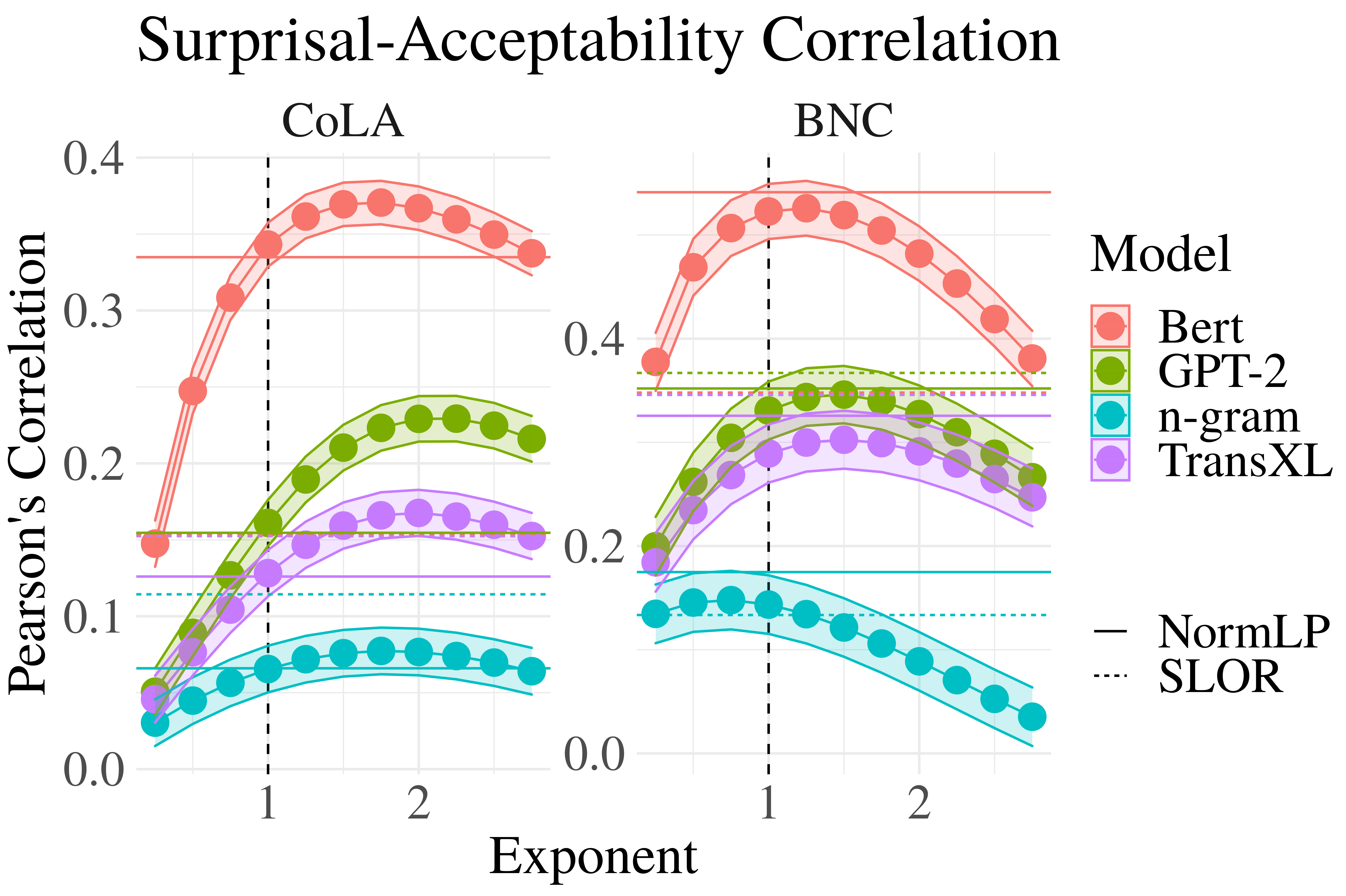
Figure 5: Fig. 1 with correlations for SLOR and NormLP predictors (from Lau et al. (2017))

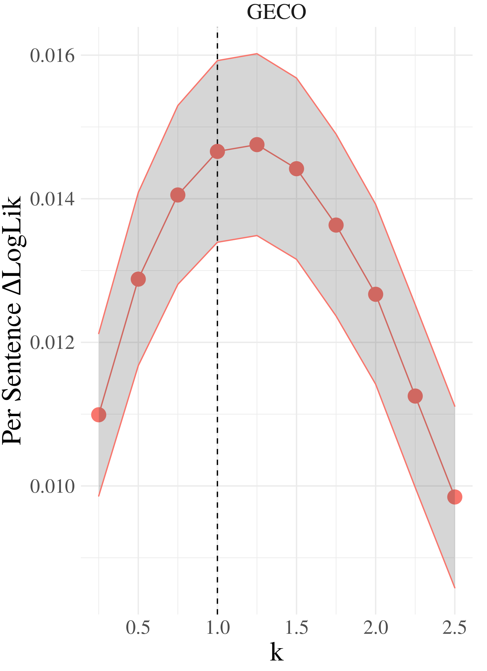
Figure 6: Same graph as in Fig. 3 for the Dutch GECO dataset. We use Dutch GPT-2 de Vries and Nissim (2021) for surprisal estimates.

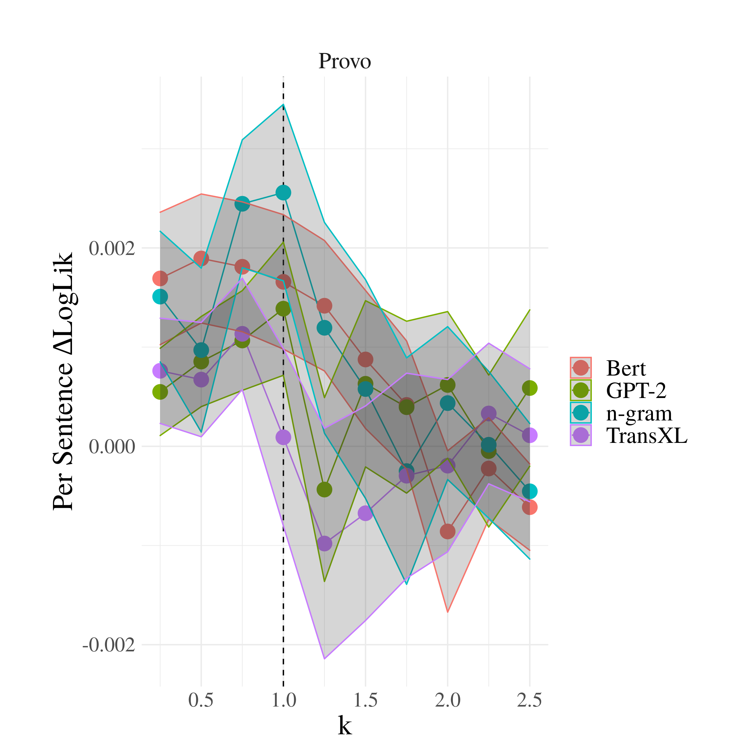
Figure 7: Same graph as in Fig. 3 for Provo albeit using (the sum of) first pass times as our reading time metric.

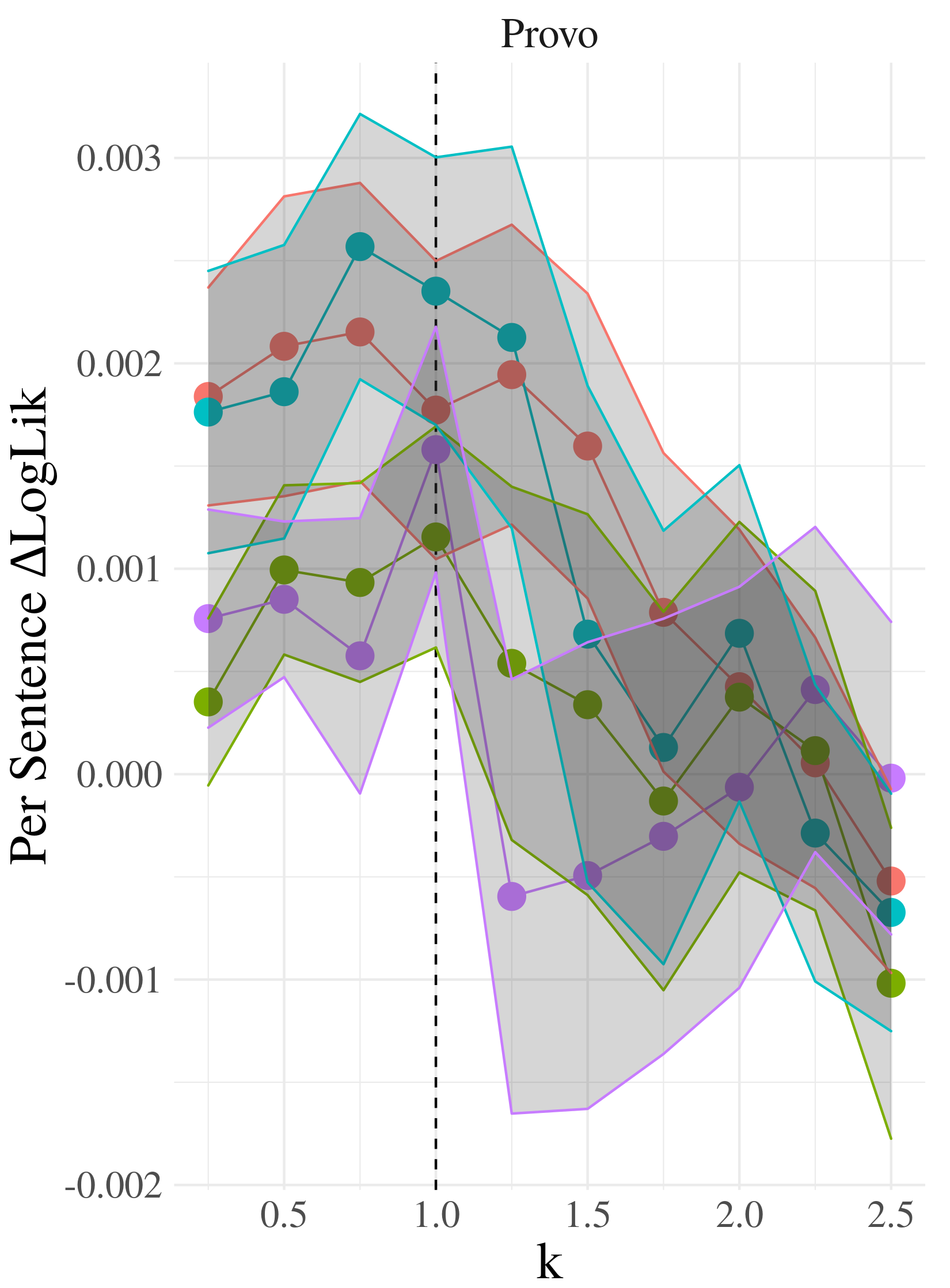
Figure 8: Same graph as in Fig. 3 for Provo albeit using (the sum of) first fixation duration times as our reading time metric.

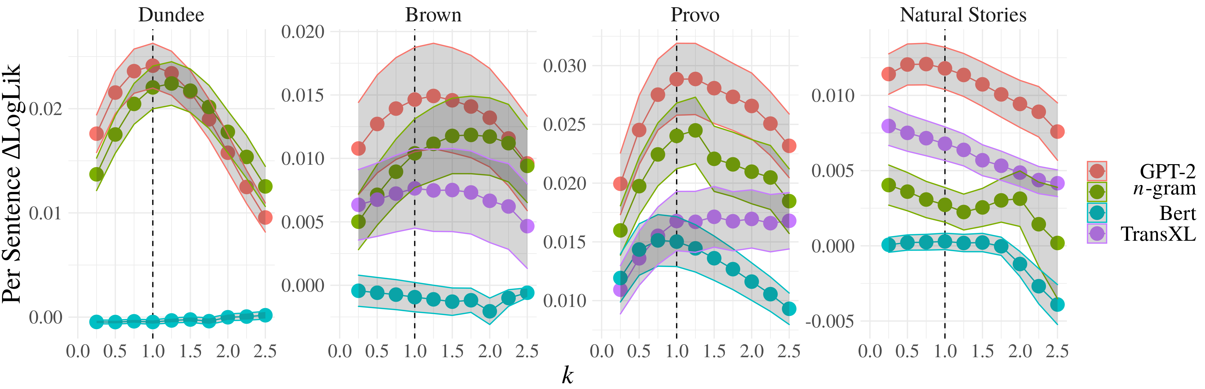
Figure 9: Version of Fig. 3 albeit with linear terms for summed unigram log-probability, total character length, and their interaction as predictors.

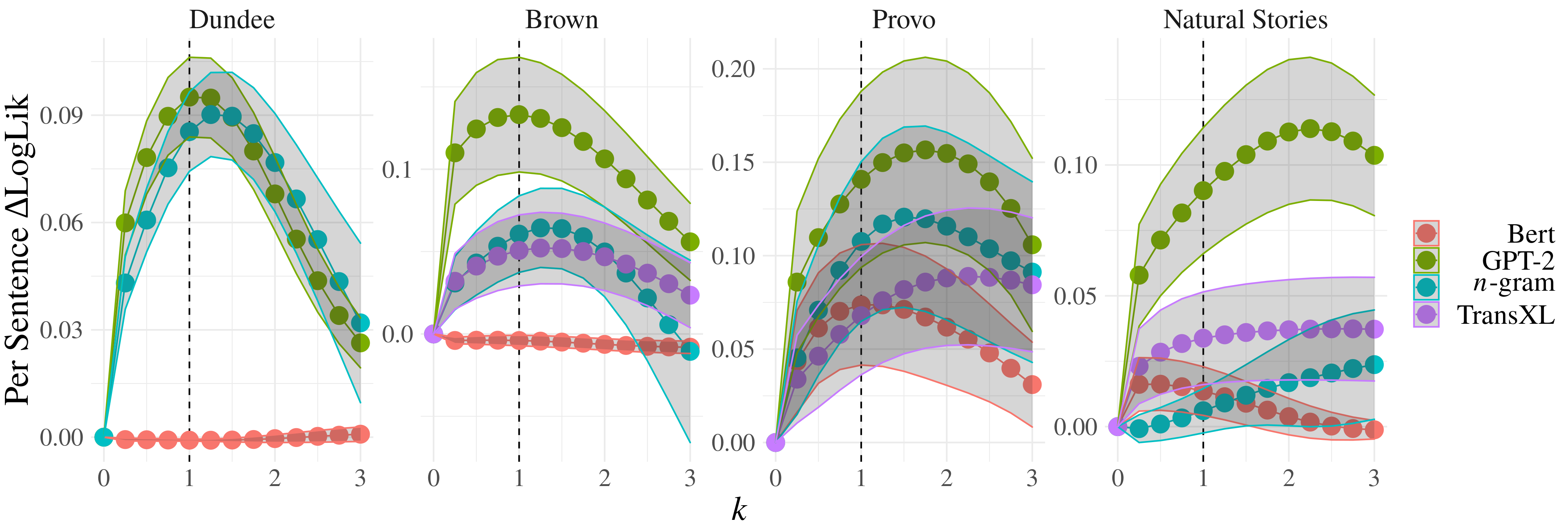
Figure 10: Version of Fig. 3 albeit with reading time data aggregated (mean across subjects) per sentence. A simple, linear model is used with the same predictors as Fig. 3

Predictor
	Dundee	Brown	Provo	NS	CoLA	bnc
$\mathrm{Super}\text{-}\mathrm{Linear}$ ($k=0.25$)	$2.08{\color[rgb]{0.0,0.0,0.5}\bf\scriptstyle\,(\pm 0.2)}$	$0.88{\color[rgb]{0.0,0.0,0.5}\bf\scriptstyle\,(\pm 0.36)}$	$0.97{\color[rgb]{0.0,0.0,0.5}\bf\scriptstyle\,(\pm 0.21)}$	$1.05{\color[rgb]{0.0,0.0,0.5}\bf\scriptstyle\,(\pm 0.11)}$	$0.9{\color[rgb]{0.0,0.0,0.5}\bf\scriptstyle\,(\pm 0.03)}$	$6.11{\color[rgb]{0.0,0.0,0.5}\bf\scriptstyle\,(\pm 0.13)}$
$\mathrm{Super}\text{-}\mathrm{Linear}$ ($k=1$)	$2.85{\color[rgb]{0.0,0.0,0.5}\bf\scriptstyle\,(\pm 0.23)}$	$1.16{\color[rgb]{0.0,0.0,0.5}\bf\scriptstyle\,(\pm 0.4)}$	$1.87{\color[rgb]{0.0,0.0,0.5}\bf\scriptstyle\,(\pm 0.29)}$	$1.08{\color[rgb]{0.0,0.0,0.5}\bf\scriptstyle\,(\pm 0.11)}$	$5.28{\color[rgb]{0.0,0.0,0.5}\bf\scriptstyle\,(\pm 0.07)}$	$13.89{\color[rgb]{0.0,0.0,0.5}\bf\scriptstyle\,(\pm 0.19)}$
$\mathrm{Super}\text{-}\mathrm{Linear}$ ($k=1.25$)	$2.83{\color[rgb]{0.0,0.0,0.5}\bf\scriptstyle\,(\pm 0.23)}$	$1.16{\color[rgb]{0.0,0.0,0.5}\bf\scriptstyle\,(\pm 0.41)}$	$2{\color[rgb]{0.0,0.0,0.5}\bf\scriptstyle\,(\pm 0.3)}$	$1.03{\color[rgb]{0.0,0.0,0.5}\bf\scriptstyle\,(\pm 0.11)}$	$5.92{\color[rgb]{0.0,0.0,0.5}\bf\scriptstyle\,(\pm 0.07)}$	$14.35{\color[rgb]{0.0,0.0,0.5}\bf\scriptstyle\,(\pm 0.19)}$
$\mathrm{Super}\text{-}\mathrm{Linear}$ ($k=1.5$)	$2.69{\color[rgb]{0.0,0.0,0.5}\bf\scriptstyle\,(\pm 0.23)}$	$1.14{\color[rgb]{0.0,0.0,0.5}\bf\scriptstyle\,(\pm 0.41)}$	$1.98{\color[rgb]{0.0,0.0,0.5}\bf\scriptstyle\,(\pm 0.3)}$	$0.98{\color[rgb]{0.0,0.0,0.5}\bf\scriptstyle\,(\pm 0.11)}$	$6.18{\color[rgb]{0.0,0.0,0.5}\bf\scriptstyle\,(\pm 0.07)}$	$14.22{\color[rgb]{0.0,0.0,0.5}\bf\scriptstyle\,(\pm 0.19)}$
$\mathrm{Super}\text{-}\mathrm{Linear}$ ($k=2$)	$2.1{\color[rgb]{0.0,0.0,0.5}\bf\scriptstyle\,(\pm 0.2)}$	$1.02{\color[rgb]{0.0,0.0,0.5}\bf\scriptstyle\,(\pm 0.39)}$	$2.01{\color[rgb]{0.0,0.0,0.5}\bf\scriptstyle\,(\pm 0.29)}$	$0.9{\color[rgb]{0.0,0.0,0.5}\bf\scriptstyle\,(\pm 0.11)}$	$6.04{\color[rgb]{0.0,0.0,0.5}\bf\scriptstyle\,(\pm 0.07)}$	$12.75{\color[rgb]{0.0,0.0,0.5}\bf\scriptstyle\,(\pm 0.18)}$
$\mathrm{Variance}$ (lang)	$1.18{\color[rgb]{0.0,0.0,0.5}\bf\scriptstyle\,(\pm 0.15)}$	$0.66{\color[rgb]{0.0,0.0,0.5}\bf\scriptstyle\,(\pm 0.32)}$	$1.59{\color[rgb]{0.0,0.0,0.5}\bf\scriptstyle\,(\pm 0.27)}$	$0.36{\color[rgb]{0.0,0.0,0.5}\bf\scriptstyle\,(\pm 0.08)}$	$5.64{\color[rgb]{0.0,0.0,0.5}\bf\scriptstyle\,(\pm 0.07)}$	$11.26{\color[rgb]{0.0,0.0,0.5}\bf\scriptstyle\,(\pm 0.17)}$
$\mathrm{Variance}$ (sent)	$0.96{\color[rgb]{0.0,0.0,0.5}\bf\scriptstyle\,(\pm 0.14)}$	$0.53{\color[rgb]{0.0,0.0,0.5}\bf\scriptstyle\,(\pm 0.28)}$	$1.57{\color[rgb]{0.0,0.0,0.5}\bf\scriptstyle\,(\pm 0.27)}$	$0.42{\color[rgb]{0.0,0.0,0.5}\bf\scriptstyle\,(\pm 0.09)}$	$1.86{\color[rgb]{0.0,0.0,0.5}\bf\scriptstyle\,(\pm 0.04)}$	$7.56{\color[rgb]{0.0,0.0,0.5}\bf\scriptstyle\,(\pm 0.14)}$
$\mathrm{LocalVariance}$	$0.9{\color[rgb]{0.0,0.0,0.5}\bf\scriptstyle\,(\pm 0.13)}$	$0.55{\color[rgb]{0.0,0.0,0.5}\bf\scriptstyle\,(\pm 0.3)}$	$1.16{\color[rgb]{0.0,0.0,0.5}\bf\scriptstyle\,(\pm 0.23)}$	$0.3{\color[rgb]{0.0,0.0,0.5}\bf\scriptstyle\,(\pm 0.07)}$	$1.44{\color[rgb]{0.0,0.0,0.5}\bf\scriptstyle\,(\pm 0.04)}$	$4.88{\color[rgb]{0.0,0.0,0.5}\bf\scriptstyle\,(\pm 0.12)}$
$\mathrm{Max}$	$0.79{\color[rgb]{0.0,0.0,0.5}\bf\scriptstyle\,(\pm 0.14)}$	$0.42{\color[rgb]{0.0,0.0,0.5}\bf\scriptstyle\,(\pm 0.31)}$	$0.33{\color[rgb]{0.0,0.0,0.5}\bf\scriptstyle\,(\pm 0.22)}$	$0.37{\color[rgb]{0.0,0.0,0.5}\bf\scriptstyle\,(\pm 0.1)}$	$1.16{\color[rgb]{0.0,0.0,0.5}\bf\scriptstyle\,(\pm 0.03)}$	$5{\color[rgb]{0.0,0.0,0.5}\bf\scriptstyle\,(\pm 0.12)}$
$\mathrm{Entropy}$ ($k=0.25$)	$1.52{\color[rgb]{0.0,0.0,0.5}\bf\scriptstyle\,(\pm 0.17)}$	$0.45{\color[rgb]{0.0,0.0,0.5}\bf\scriptstyle\,(\pm 0.26)}$	$1.34{\color[rgb]{0.0,0.0,0.5}\bf\scriptstyle\,(\pm 0.22)}$	$0.31{\color[rgb]{0.0,0.0,0.5}\bf\scriptstyle\,(\pm 0.12)}$	$0.02{\color[rgb]{0.0,0.0,0.5}\bf\scriptstyle\,(\pm 0)}$	$0.03{\color[rgb]{0.0,0.0,0.5}\bf\scriptstyle\,(\pm 0.01)}$
$\mathrm{Entropy}$ ($k=1$) Shannon	$-0.01{\color[rgb]{0.0,0.0,0.5}\bf\scriptstyle\,(\pm 0)}$	$0{\color[rgb]{0.0,0.0,0.5}\bf\scriptstyle\,(\pm 0.01)}$	$0.01{\color[rgb]{0.0,0.0,0.5}\bf\scriptstyle\,(\pm 0)}$	$0{\color[rgb]{0.0,0.0,0.5}\bf\scriptstyle\,(\pm 0)}$	$0{\color[rgb]{0.0,0.0,0.5}\bf\scriptstyle\,(\pm 0)}$	$7.9{\color[rgb]{0.0,0.0,0.5}\bf\scriptstyle\,(\pm 0.14)}$
$\mathrm{Entropy}$ ($k=2$) Renyi	$-0.01{\color[rgb]{0.0,0.0,0.5}\bf\scriptstyle\,(\pm 0)}$	$0{\color[rgb]{0.0,0.0,0.5}\bf\scriptstyle\,(\pm 0.01)}$	$0{\color[rgb]{0.0,0.0,0.5}\bf\scriptstyle\,(\pm 0.01)}$	$0{\color[rgb]{0.0,0.0,0.5}\bf\scriptstyle\,(\pm 0)}$	$0{\color[rgb]{0.0,0.0,0.5}\bf\scriptstyle\,(\pm 0)}$	$8.38{\color[rgb]{0.0,0.0,0.5}\bf\scriptstyle\,(\pm 0.14)}$

Table 3: $\Delta\mathrm{LogLik}$ in $10\text{e-}2$ nats, as in Tab. 1 albeit with different baseline predictors for reading time data and with using BERT for surprisal estimates for acceptability judgments. Along with the predictors specified in Tab. 1, models for reading times here also contain predictors for unigram log-probability, total character length, and the interaction of the two (reading times). We see largely the same trends as in Tab. 1.

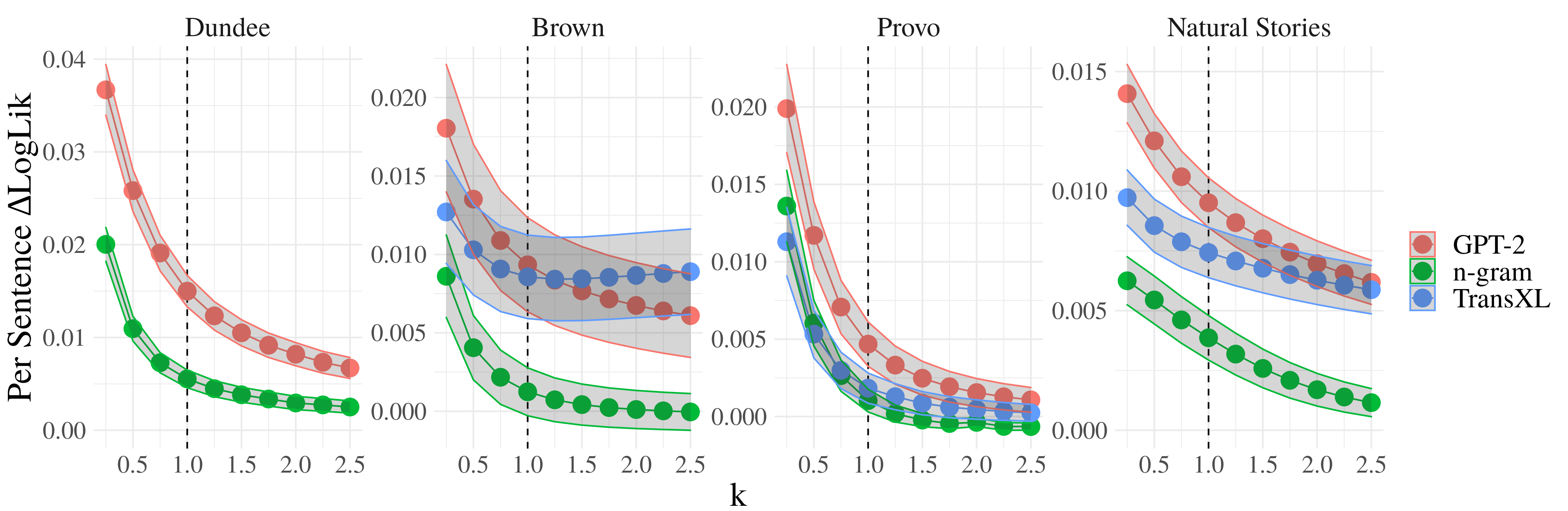
Figure 11: Version of Fig. 3 albeit using probabilities instead of surprisal in the summation $\sum_{n=1}^{N}s(u_{n})$. Note that the magnitude of $\Delta\mathrm{LogLik}$ is smaller than when using surprisal, indicating the superior predictive power of the latter. This stands in contrast to the experimental findings of Brothers and Kuperberg (2021).

References

- Aylett and Turk (2004) Matthew Aylett and Alice Turk. 2004. The smooth signal redundancy hypothesis: A functional explanation for relationships between redundancy, prosodic prominence, and duration in spontaneous speech. Language and Speech, 47(1):31–56.
- Bell et al. (2003) Alan Bell, Daniel Jurafsky, Eric Fosler-Lussier, Cynthia Girand, Michelle Gregory, and Daniel Gildea. 2003. Effects of disfluencies, predictability, and utterance position on word form variation in English conversation. The Journal of the Acoustical Society of America, 113(2):1001–1024.
- Bloem (2016) Jelke Bloem. 2016. Testing the processing hypothesis of word order variation using a probabilistic language model. In Proceedings of the Workshop on Computational Linguistics for Linguistic Complexity (CL4LC), pages 174–185. The COLING 2016 Organizing Committee.
- Brothers and Kuperberg (2021) Trevor Brothers and Gina R. Kuperberg. 2021. Word predictability effects are linear, not logarithmic: Implications for probabilistic models of sentence comprehension. Journal of Memory and Language, 116:104174.
- Brouwer et al. (2010) Harm Brouwer, Hartmut Fitz, and John Hoeks. 2010. Modeling the noun phrase versus sentence coordination ambiguity in Dutch: Evidence from surprisal theory. In Proceedings of the 2010 Workshop on Cognitive Modeling and Computational Linguistics, pages 72–80. Association for Computational Linguistics.
- Collins (2014) Michael Xavier Collins. 2014. Information density and dependency length as complementary cognitive models. Journal of Psycholinguistic Research, 43(5):651–681.
- Cop et al. (2017) Uschi Cop, Nicolas Dirix, Denis Drieghe, and Wouter Duyck. 2017. Presenting GECO: An eyetracking corpus of monolingual and bilingual sentence reading. Behavior Research Methods, 49(2):602–615.
- Coupé et al. (2019) Christophe Coupé, Yoon Mi Oh, Dan Dediu, and François Pellegrino. 2019. Different languages, similar encoding efficiency: Comparable information rates across the human communicative niche. Science Advances, 5(9).
- Dai et al. (2019) Zihang Dai, Zhilin Yang, Yiming Yang, Jaime Carbonell, Quoc Le, and Ruslan Salakhutdinov. 2019. Transformer-XL: Attentive language models beyond a fixed-length context. In Proceedings of the 57th Annual Meeting of the Association for Computational Linguistics, pages 2978–2988. Association for Computational Linguistics.
- de Vries and Nissim (2021) Wietse de Vries and Malvina Nissim. 2021. As good as new. how to successfully recycle English GPT-2 to make models for other languages. In Findings of the Association for Computational Linguistics: ACL-IJCNLP 2021, pages 836–846. Association for Computational Linguistics.
- Demberg and Keller (2008) Vera Demberg and Frank Keller. 2008. Data from eye-tracking corpora as evidence for theories of syntactic processing complexity. Cognition, 109(2):193–210.
- Devlin et al. (2019) Jacob Devlin, Ming-Wei Chang, Kenton Lee, and Kristina Toutanova. 2019. BERT: Pre-training of deep bidirectional transformers for language understanding. In Proceedings of the 2019 Conference of the North American Chapter of the Association for Computational Linguistics: Human Language Technologies, Volume 1 (Long and Short Papers), pages 4171–4186. Association for Computational Linguistics.
- Fenk and Fenk (1980) August Fenk and Gertraud Fenk. 1980. Konstanz im Kurzzeitgedächtnis - Konstanz im sprachlichen Informationsfluß? Zeitschrift für Experimentelle und Angewandte Psychologie, 27(3):400–414.
- Fernandez Monsalve et al. (2012) Irene Fernandez Monsalve, Stefan L. Frank, and Gabriella Vigliocco. 2012. Lexical surprisal as a general predictor of reading time. In Proceedings of the 13th Conference of the European Chapter of the Association for Computational Linguistics, pages 398–408. Association for Computational Linguistics.
- Fossum and Levy (2012) Victoria Fossum and Roger Levy. 2012. Sequential vs. hierarchical syntactic models of human incremental sentence processing. In Proceedings of the 3rd Workshop on Cognitive Modeling and Computational Linguistics (CMCL 2012), pages 61–69. Association for Computational Linguistics.
- Frank and Jaeger (2008) A. F. Frank and T. Jaeger. 2008. Speaking rationally: Uniform information density as an optimal strategy for language production. In the Annual Meeting of the Cognitive Science Society.
- Frank and Bod (2011) Stefan L. Frank and Rens Bod. 2011. Insensitivity of the human sentence-processing system to hierarchical structure. Psychological Science, 22(6):829–834.
- Frank et al. (2013) Stefan L. Frank, Leun J. Otten, Giulia Galli, and Gabriella Vigliocco. 2013. Word surprisal predicts n400 amplitude during reading. In Proceedings of the 51st Annual Meeting of the Association for Computational Linguistics (Volume 2: Short Papers), pages 878–883. Association for Computational Linguistics.
- Futrell et al. (2018) Richard Futrell, Edward Gibson, Harry J. Tily, Idan Blank, Anastasia Vishnevetsky, Steven Piantadosi, and Evelina Fedorenko. 2018. The Natural Stories Corpus. In Proceedings of the Eleventh International Conference on Language Resources and Evaluation (LREC 2018). European Language Resources Association.
- Genzel and Charniak (2002) Dmitriy Genzel and Eugene Charniak. 2002. Entropy rate constancy in text. In Proceedings of the 40th Annual Meeting of the Association for Computational Linguistics, pages 199–206. Association for Computational Linguistics.
- Goodkind and Bicknell (2018a) Adam Goodkind and Klinton Bicknell. 2018a. Predictive power of word surprisal for reading times is a linear function of language model quality. In Proceedings of the 8th Workshop on Cognitive Modeling and Computational Linguistics (CMCL 2018), pages 10–18.
- Goodkind and Bicknell (2018b) Adam Goodkind and Klinton Bicknell. 2018b. Predictive power of word surprisal for reading times is a linear function of language model quality. In Proceedings of the 8th Workshop on Cognitive Modeling and Computational Linguistics (CMCL 2018), pages 10–18. Association for Computational Linguistics.
- Hale (2001) John Hale. 2001. A probabilistic Earley parser as a psycholinguistic model. In Second Meeting of the North American Chapter of the Association for Computational Linguistics.
- Heafield (2011) Kenneth Heafield. 2011. KenLM: Faster and smaller language model queries. In Proceedings of the Sixth Workshop on Statistical Machine Translation, pages 187–197. Association for Computational Linguistics.
- Jaeger (2010) T. Jaeger. 2010. Redundancy and reduction: Speakers manage syntactic information density. Cognitive Psychology, 61:23–62.
- Jain et al. (2018) Ayush Jain, Vishal Singh, Sidharth Ranjan, Rajakrishnan Rajkumar, and Sumeet Agarwal. 2018. Uniform Information Density effects on syntactic choice in Hindi. In Proceedings of the Workshop on Linguistic Complexity and Natural Language Processing, pages 38–48. Association for Computational Linguistics.
- Kennedy et al. (2003) Alan Kennedy, Robin Hill, and Joel Pynte. 2003. The Dundee Corpus. In Proceedings of the 12th European Conference on Eye Movements.
- Kuribayashi et al. (2021) Tatsuki Kuribayashi, Yohei Oseki, Takumi Ito, Ryo Yoshida, Masayuki Asahara, and Kentaro Inui. 2021. Lower perplexity is not always human-like. In Proceedings of the 59th Annual Meeting of the Association for Computational Linguistics and the 11th International Joint Conference on Natural Language Processing, pages 5203–5217. Association for Computational Linguistics.
- Lau et al. (2017) Jey Han Lau, Alexander Clark, and Shalom Lappin. 2017. Grammaticality, acceptability, and probability: A probabilistic view of linguistic knowledge. Cognitive Science, 41(5):1202–1241.
- Levy (2005) Roger Levy. 2005. Probabilistic Models of Word Order and Syntactic Discontinuity. Ph.D. thesis, Stanford University.
- Levy (2008) Roger Levy. 2008. Expectation-based syntactic comprehension. Cognition, 106(3):1126–1177.
- Levy and Jaeger (2007) Roger Levy and T. Florian Jaeger. 2007. Speakers optimize information density through syntactic reduction. In Advances in Neural Information Processing Systems, volume 19. MIT Press.
- Levy (2018) Roger P. Levy. 2018. Communicative efficiency, Uniform Information Density, and the Rational Speech Act Theory. In 40th Annual Meeting of the Cognitive Science Society, pages 684–689. Cognitive Science Society.
- Luke and Christianson (2018) Steven G. Luke and Kiel Christianson. 2018. The Provo Corpus: A large eye-tracking corpus with predictability norms. Behavior Research Methods, 50(2):826–833.
- Mahowald et al. (2013) Kyle Mahowald, Evelina Fedorenko, Steven T. Piantadosi, and Edward Gibson. 2013. Info/information theory: Speakers choose shorter words in predictive contexts. Cognition, 126(2):313–318.
- Meister et al. (2020) Clara Meister, Ryan Cotterell, and Tim Vieira. 2020. If beam search is the answer, what was the question? In Proceedings of the 2020 Conference on Empirical Methods in Natural Language Processing (EMNLP), pages 2173–2185. Association for Computational Linguistics.
- Merity et al. (2017) Stephen Merity, Caiming Xiong, James Bradbury, and Richard Socher. 2017. Pointer sentinel mixture models. In 5th International Conference on Learning Representations.
- Mitchell et al. (2010) Jeff Mitchell, Mirella Lapata, Vera Demberg, and Frank Keller. 2010. Syntactic and semantic factors in processing difficulty: An integrated measure. In Proceedings of the 48th Annual Meeting of the Association for Computational Linguistics, pages 196–206. Association for Computational Linguistics.
- Ney et al. (1994) Hermann Ney, Ute Essen, and Reinhard Kneser. 1994. On structuring probabilistic dependences in stochastic language modelling. Computer Speech and Language, 8(1):1–38.
- Nikkarinen et al. (2021) Irene Nikkarinen, Tiago Pimentel, Damián Blasi, and Ryan Cotterell. 2021. Modelling the unigram distribution. In Findings of the Association for Computational Linguistics: ACL-IJCNLP 2021, pages 3721–3729. Association for Computational Linguistics.
- Pellegrino et al. (2011) François Pellegrino, Ioana Chitoran, Egidio Marsico, and Christophe Coupé. 2011. A cross-language perspective on speech information rate. Language, 87(3):539–558.
- Pijpops et al. (2018) Dirk Pijpops, Dirk Speelman, Stefan Grondelaers, and Freek Van de Velde. 2018. Comparing explanations for the complexity principle: evidence from argument realization. Language and Cognition, 10(3):514–543.
- Pimentel et al. (2021) Tiago Pimentel, Clara Meister, Elizabeth Salesky, Simone Teufel, Damián Blasi, and Ryan Cotterell. 2021. A surprisal–duration trade-off across and within the world's languages. In Proceedings of the 2021 Conference on Empirical Methods in Natural Language Processing. Association for Computational Linguistics.
- Radford et al. (2019) Alec Radford, Jeffrey Wu, Rewon Child, David Luan, Dario Amodei, Ilya Sutskever, et al. 2019. Language models are unsupervised multitask learners. OpenAI blog, 1(8):9.
- Rayner (1998) Keith Rayner. 1998. Eye movements in reading and information processing: 20 years of research. Psychological Bulletin, 124(3):372–422.
- Rényi (1961) Alfréd Rényi. 1961. On measures of entropy and information. In Proceedings of the Fourth Berkeley Symposium on Mathematical Statistics and Probability, Volume 1: Contributions to the Theory of Statistics, pages 547–561. University of California Press.
- Schrimpf et al. (2020) Martin Schrimpf, Idan Blank, Greta Tuckute, Carina Kauf, Eghbal A Hosseini, Nancy Kanwisher, Joshua Tenenbaum, and Evelina Fedorenko. 2020. The neural architecture of language: Integrative reverse-engineering converges on a model for predictive processing. BioRxiv.
- Sennrich et al. (2016) Rico Sennrich, Barry Haddow, and Alexandra Birch. 2016. Neural machine translation of rare words with subword units. In Proceedings of the 54th Annual Meeting of the Association for Computational Linguistics, pages 1715–1725. Association for Computational Linguistics.
- Shannon (1948) Claude E. Shannon. 1948. A mathematical theory of communication. The Bell System Technical Journal, 27(3):379–423.
- Sikos et al. (2017) Les Sikos, Clayton Greenberg, Heiner Drenhaus, and Matthew W Crocker. 2017. Information density of encodings: The role of syntactic variation in comprehension. In 39th Annual Meeting of the Cognitive Science Society. Cognitive Science Society.
- Smith and Levy (2013) Nathaniel J. Smith and Roger Levy. 2013. The effect of word predictability on reading time is logarithmic. Cognition, 128(3):302–319.
- Topolinski and Strack (2009) Sascha Topolinski and Fritz Strack. 2009. The architecture of intuition: fluency and affect determine intuitive judgments of semantic and visual coherence and judgments of grammaticality in artificial grammar learning. Journal of Experimental Psychology: General, 138(1):39.
- Torabi Asr and Demberg (2015) Fatemeh Torabi Asr and Vera Demberg. 2015. Uniform surprisal at the level of discourse relations: Negation markers and discourse connective omission. In Proceedings of the 11th International Conference on Computational Semantics, pages 118–128. Association for Computational Linguistics.
- Warstadt et al. (2019) Alex Warstadt, Amanpreet Singh, and Samuel R. Bowman. 2019. Neural network acceptability judgments. Transactions of the Association for Computational Linguistics, 7:625–641.
- Wei et al. (2021) Jason Wei, Clara Meister, and Ryan Cotterell. 2021. A cognitive regularizer for language modeling. In Proceedings of the 59th Annual Meeting of the Association for Computational Linguistics and the 10th International Joint Conference on Natural Language Processing, pages 5191–5202. Association for Computational Linguistics.
- Wilcox et al. (2020) Ethan Gotlieb Wilcox, Jon Gauthier, Jennifer Hu, Peng Qian, and Roger Levy. 2020. On the predictive power of neural language models for human real-time comprehension behavior. In Proceedings of the 42nd Annual Meeting of the Cognitive Science Society, pages 1707–1713. Cognitive Science Society.
- Wolf et al. (2020) Thomas Wolf, Lysandre Debut, Victor Sanh, Julien Chaumond, Clement Delangue, Anthony Moi, Pierric Cistac, Tim Rault, Remi Louf, Morgan Funtowicz, Joe Davison, Sam Shleifer, Patrick von Platen, Clara Ma, Yacine Jernite, Julien Plu, Canwen Xu, Teven Le Scao, Sylvain Gugger, Mariama Drame, Quentin Lhoest, and Alexander Rush. 2020. Transformers: State-of-the-art natural language processing. In Proceedings of the 2020 Conference on Empirical Methods in Natural Language Processing: System Demonstrations, pages 38–45. Association for Computational Linguistics.
- Zhan and Levy (2018) Meilin Zhan and Roger Levy. 2018. Comparing theories of speaker choice using a model of classifier production in Mandarin Chinese. In Proceedings of the 2018 Conference of the North American Chapter of the Association for Computational Linguistics: Human Language Technologies, pages 1997–2005. Association for Computational Linguistics.
- Zhan and Levy (2019) Meilin Zhan and Roger P. Levy. 2019. Availability-based production predicts speakers' real-time choices of Mandarin classifiers. In 41st Annual Meeting of the Cognitive Science Society, pages 1268–1274. Cognitive Science Society.