Nonlinear spectroscopy of excitonic states in transition metal dichalcogenides

Abstract

Second-harmonic generation (SHG) is a well-known nonlinear spectroscopy method to probe electronic structure, specifically, in transition metal dichalcogenide (TMDC) monolayers. This work investigates the nonlinear dynamics of a strongly excited TMDC monolayer by solving the time evolution equations for the density matrix. It is shown that the presence of excitons qualitatively changes the nonlinear dynamics leading, in particular, to a huge enhancement of the nonlinear signal as a function of the dielectric environment. It is also shown that the SHG polarization angular diagram and its dependence on the driving strength are very sensitive to the type of exciton state. This sensitivity suggests that SHG spectroscopy is a convenient tool for analyzing the fine structure of excitonic states.

I Introduction

Second-harmonic generation (SHG) Boyd (2020) is a powerful tool for studying optical properties of a variety of materials, including semiconductors Ghimire et al. (2010); Chin et al. (2001); Belyanin et al. (2005), molecules Prasad and Williams (1991), carbon nanotubes Dominicis et al. (2004); Murakami and Kono (2009); Kono (2013), and layered transition metal dichalcogenide (TMDC) structures Kumar et al. (2013); Malard et al. (2013); Yin et al. (2014); Clark et al. (2014); Hsu et al. (2014); Janisch et al. (2014); Jiang et al. (2014); Liu et al. (2016); Säynätjoki et al. (2017); Autere et al. (2018); Mennel et al. (2018, 2019); Stiehm et al. (2019); Maragkakis et al. (2019); Lin et al. (2019); Zhang et al. (2020); Khan et al. (2020); Ho et al. (2020). The nonlinear nature of SHG allows one to probe material characteristics on a level that usually evades linear spectroscopy methods. For example, the sensitivity of SHG measurement to spatial and time-reversal symmetries makes it handy for uncovering phenomena that are out of the reach of more traditional optical methods Heinz (1991), including magnetic ordering Fiebig et al. (1998); Shree et al. (2020) and hidden phase transitions Fiebig et al. (2005). Recently SHG spectroscopy has been applied to map strain profiles with the spatial resolution surpassing the optical diffraction limit Mennel et al. (2018, 2019).

In TMDC monolayers Ma et al. (2020), the SHG method has been applied to investigate the symmetry of crystal structures Kumar et al. (2013); Malard et al. (2013); Li et al. (2013); Yin et al. (2014); Clark et al. (2014); Hsu et al. (2014); Maragkakis et al. (2019), detect charged molecules Yu et al. (2016), map strains Mennel et al. (2018, 2019); Khan et al. (2020), and probe valley polarization Wehling et al. (2015); Hipolito and Pereira (2017); Ho et al. (2020). SHG signal is very sensitive to electronic excitations, making it a powerful tool for studying the band structure and interband transitions. The SHG is a unique tool to fill the gap left by the Raman and photoluminescence spectroscopy, and it is well suited to study atomic and electronic structures of two-dimensional (2D) layered TMDC systems Zhang et al. (2020). Experiments with layered $\text{WSe}_{2}$ on hexagonal boron nitride (h-BN) substrates Lin et al. (2019), $\text{WS}_{2}$ Janisch et al. (2014), $\text{MoS}_{2}$ monolayers Mennel et al. (2018) and bilayers Jiang et al. (2014), and a 2D GaSe crystal Zhou et al. (2015) revealed a conventional six-leaf pattern of the SHG signal angular dependence, which is commonly employed to determine the orientation of the monolayer crystals Kumar et al. (2013); Malard et al. (2013); Li et al. (2013); Yin et al. (2014); Clark et al. (2014); Hsu et al. (2014); Maragkakis et al. (2019). Distortions of that symmetry, e.g., by an applied tensile strain, give rise to a distorted SHG angular dependence Mennel et al. (2019).

We show here that the SHG signal’s sensitivity to the excitation field intensity, frequency, and polarization can be used to probe the nature of electronic states in TMDC materials on a much more detailed level than linear spectroscopy allows. We find that unlike most materials, in TMDC, both linear and quadratic terms in the vector potential of the excitation laser light must be included to describe correctly nonlinear light-matter interaction and nonlinear dynamics. In particular, we find that the competition between the linear and quadratic terms as a function of the laser power leads to peculiar changes in the polarization diagrams of the SHG pattern. Unlike the linear response spectra, the interpretation of the SHG signals involves theoretical analysis that cannot be limited to calculating the transition energies and rates but requires one to investigate the nonlinear dynamics of the system, which is a much more complex problem. In some cases, the analysis can be simplified by employing the dynamical perturbation theory to calculate the second harmonic. However, the perturbative approach fails in the most physically interesting case of strong excitations and highly nonlinear dynamics or when the higher-order harmonics are essential. It is also not convenient when one has a mixture of excitations of different nature. In those cases, the complete nonlinear dynamical problem must be solved. For TMDC monolayers, it is often solved for single-particle excitations treated within the semi-classical approximation. This approach is well justified, e.g., when the driving field of extra-strong intensity produces many high harmonics.

In many other relevant situations, such as SHG, the field strength is not strong enough to ionize excitons, and single-particle approximation may become inadequate, although the dynamics is still nonlinear. In 2D materials, this regime is easily accessible because of the strong Coulomb interaction enhancing the many-body effects. It facilitates the formation of tightly bound many-particle excitonic complexes, manifested in the linear optical spectra of 2D TMDC structures Mak et al. (2010); Splendiani et al. (2010); Chernikov et al. (2014); Seyler et al. (2015); Wang et al. (2015, 2018). The exciton-related effects should also be visible in nonlinear dynamics, in particular, SHG. However, investigations of the nonlinear dynamics associated with the excitonic states are currently in an infant stage. Contemporary research focuses mainly on the linear response Cheiwchanchamnangij and Lambrecht (2012); Ramasubramaniam (2012); Qiu et al. (2013); Berkelbach et al. (2013); Qiu et al. (2015); Zhumagulov et al. (2020a, b, 2021). Analysis of the nonlinear effects such as SHG mainly concentrates on perturbative calculations Trolle et al. (2014); Grüning and Attaccalite (2014); Glazov et al. (2017); Kolos et al. (2021). A more elaborate investigation of the exciton dynamics in TMDC can be done by solving dynamics equations for the pertinent elements of the density matrix Richter and Knorr (2010) obtained using the dynamics control truncation (DCT) approximation Axt and Kuhn (2004).

In this work, we investigate the role of exciton states in the SHG of TMDC monolayers. Using the solution for the Liouville - von Neumann (LvN) equation, we obtain SHG angular polarization diagrams and study their dependence on the frequency and intensity of the excitation pulse. The results reveal an extraordinary sensitivity of the SHG signal to the type of exciton states. Our findings are general, and similar SHG polarization diagrams are obtained for monolayers of common TMDC’s ($\text{MoS}_{2}$, $\text{MoSe}_{2}$, $\text{WS}_{2}$, and $\text{WSe}_{2}$) with a qualitatively similar two valley band structure. Our results offer the tantalizing possibility of SHG spectroscopy of exciton states that can be used to probe and detect finer details of excitonic states that conventional optical methods cannot capture.

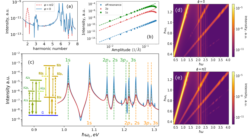
Figure 1: (a) Spectral intensity of the nonlinear response $I_{\omega_{L},\omega}$ calculated at $f=0.5\AA^{-1}$ and $\hbar\omega_{L}=0.35$eV (off-resonance) for polarization angle $\phi=0$ (blue) and $\phi=\pi/2$ (red). (b) SHG intensity $I_{\omega_{L},2\omega_{L}}$ calculated for the off-resonant driving with $\hbar\omega_{L}=0.35$eV (blue circles), in resonance with the $A1s$ exciton state (green squares), and in resonance with the $A2p_{+}$ exciton state (red triangles). Dashed lines show the perturbation theory result $I\propto f^{4}$. (c) SHG intensity as a function of $\hbar\omega_{L}$ calculated at $f=0.1\AA^{-1}$ without dephasing ($\gamma=0$, blue line) and with dephasing ($\gamma=10$meV, red line). A and B excitons are marked by green and orange dashed lines. The inset is a schematic energy diagram (not to scale) of optically active low-energy excitons in a $\text{MoS}_{2}$ monolayer. Solid arrows mark transitions allowed in a rotationally invariant system; dashed lines are warping mediated transitions. (d-e) Color density high harmonic intensity spectrum as a function of the driving frequency $I_{\omega_{L},\omega}$ calculated for two polarization angles $\phi=\pi/2$ and $0$, respectively.

II Dynamics of exciton states

The analysis of the harmonic generation is done by employing the formalism of the density matrix where we solve the LvN equation,

$$\frac{d\varrho}{dt}=-\frac{\mathbbm{i}}{\hbar}\big{[}H,\varrho\big{]}+{\cal L}[\varrho],$$ (1)

where $\varrho$ is the density matrix, $H$ is the Hamiltonian of the system, and the non-Hamiltonian contribution ${\cal L}$ accounts for the losses. Since we are interested in the exciton contribution to the dynamics, we consider the two-particle Hamiltonian. It contains two contributions $H=H_{ex}+H_{f}$ where $H_{ex}$ is the part describing the exciton states; and $H_{f}$ is the interaction between the excitons and the driving field. The losses are taken into account by using the phenomenological Lindblad approach where the non-Hamiltonian part of the LvN equation reads as

$${\cal L}=\sum_{a}\gamma_{a}\left[{\cal L}_{a}\rho{\cal L}_{a}^{\dagger}-\frac{1}{2}\left(\rho{\cal L}_{a}^{\dagger}{\cal L}_{a}+{\cal L}_{a}^{\dagger}{\cal L}_{a}\rho\right)\right],$$ (2)

with ${\cal L}_{a}$ and $\gamma_{a}$ being an operator and rate corresponding to a loss channel $a$. In this work, we account only for the pure dephasing mechanism, for which the operators ${\cal L}_{a}=|a\rangle\langle a|$ are diagonal in the basis of exciton states $a$. The resulting LvN equation is solved using a basis of two-particle exciton eigenstates, which are in turn calculated using conduction and valence band single-particle states of a TMDC material as a basis.

II.1 Single-particle states

Single-particle states are obtained from the massive Dirac model Hamiltonian, which takes into account the trigonal warping and spin-orbit coupling Xiao et al. (2012); Kormányos et al. (2013, 2015). It yields a good approximation for the low-lying states of a TMDC monolayer. The Hamiltonian reads as

$$H_{0}({\bf k}) =\frac{\Delta}{2}\sigma_{z}+\hbar v_{F}\tau(k_{x}\sigma_{x}+\tau k_{y}\sigma_{y})$$

$$+\frac{\tau s}{2}\big{\{}\lambda_{c}(\sigma_{z}+\sigma_{0})-\lambda_{v}(\sigma_{z}-\sigma_{0})\big{\}}$$

$$+\kappa\left\{\left(k_{x}^{2}-k_{y}^{2}\right)\sigma_{x}+2\tau k_{x}k_{y}\sigma_{y}\right\},$$ (3)

where $\sigma_{i}$ are the Pauli matrices ($\sigma_{0}$ is the unity matrix), ${\bf k}=(k_{x},k_{y})$ are the electron momentum components, $\tau=\pm 1$ is the valley index, $s=\pm 1$ denotes charge carrier spin, $v_{F}$ is the Fermi velocity, $\Delta$ is the gap between the conduction and the valence bands, and $\lambda_{c,v}$ are the spin splittings of the conduction $c$ and valence $v$ bands. The Fermi velocity is given as $\hbar v_{F}=\sqrt{\Delta/2m}$ Zhumagulov et al. (2021), and the trigonal warping constant is determined as $\kappa=-\sqrt{3}/24\hbar v_{F}a$ Kormányos et al. (2013); Taghizadeh and Pedersen (2019). Finally, we assume the following model to describe the dependence of the bandgap on the dielectric environment Cho and Berkelbach (2018)

$$\Delta =\Delta_{0}+\frac{e^{2}}{2\epsilon d}\Big{[}\frac{L_{2}+L_{1}}{\sqrt{L_{2}L_{1}}}\text{tanh}^{-1}(\sqrt{L_{2}L_{1}})$$

$$-\text{ln}(1-L_{2}L_{1})\Big{]},\quad L_{i}=\frac{\epsilon-\epsilon_{i}}{\epsilon+\epsilon_{i}},$$ (4)

where $\epsilon$ is the bulk dielectric constant of the TMDC material, $\Delta_{0}$ is its bulk bandgap, $\epsilon_{i=1,2}$ are dielectric constants of the lower and upper dielectric environment, and $d$ is the monolayer thickness. Eigenstates of the Dirac Hamiltonian are classified as quasi-electrons $|c{\bf k}\rangle$ with energies $\varepsilon_{c{\bf k}}$ above the gap and quasi-holes $|v{\bf k}\rangle$ with energies $\varepsilon_{v{\bf k}}$ below the gap. Indices $c$ and $v$ denote all state quantum numbers except for the quasimomentum ${\bf k}$. Monolayers of semiconductors $\text{MoS}_{2}$, $\text{MoSe}_{2}$, $\text{WS}_{2}$, and $\text{WSe}_{2}$ have a similar crystal configuration and qualitatively similar energy dispersion of the lowest energy single-particle states. The effective Dirac model parameters for those materials are obtained by fitting results of the first-principle band structure calculations and are summarized in Table 1.

	$a$	$d$	$\epsilon$	$\Delta_{0}$	$m$	$\lambda_{c}$	$\lambda_{v}$
MoS2	3.185	6.12	16.3	2.087	0.520	-1.41	74.60
MoSe2	3.319	6.54	17.9	1.817	0.608	-10.45	93.25
WS2	3.180	6.14	14.6	2.250	0.351	15.72	213.46
WSe2	3.319	6.52	16.0	1.979	0.379	19.85	233.07

Table 1: Model parameters for TMDC monolayers. Lattice constants $a$ (Å), effective masses $m$, and spin-orbit coupling constants $\lambda_{c,v}$ (meV) are taken from Ref. Zollner et al. (2019), monolayer thicknesses $d$ (Å) and static dielectric constants $\epsilon$ are from Ref. Laturia et al. (2018), and $\Delta_{0}$ (eV) is from Ref. Zhang et al. (2016).

With additional contributions due to the trigonal warping, the minimal coupling model describes the interaction between quasiparticles and the driving electromagnetic field. We use a common assumption that the external field has a very large wavelength compared with other system characteristic sizes. Using this assumption, we obtain the following interaction Hamiltonian for the states of momentum ${\bf k}$ Sipe and Ghahramani (1993):

$$H_{f}({\bf k})=-\frac{e}{c\hbar}\sum_{\alpha}p^{\alpha}_{\bf k}A_{\alpha}+\frac{e^{2}}{2c^{2}\hbar^{2}}\sum_{\alpha\beta}q^{\alpha\beta}_{\bf k}A_{\alpha}A_{\beta},$$ (5)

where A is the field vector potential $e$ is the electron charge, $c$ is the speed of light, and the coefficients of the linear and quadratic interaction terms are obtained as derivatives:

$$p^{\alpha}_{\bf k}=\frac{\partial H_{0}({\bf k})}{\partial k_{\alpha}},\quad q^{\alpha\beta}_{\bf k}=\frac{\partial^{2}H_{0}({\bf k})}{\partial k_{\alpha}\partial k_{\beta}}.$$ (6)

Notice that unlike the Schrodinger equation with the quadratic dispersion, the term with the second power of the field facilitates transitions between single-particle states and thus cannot be neglected.

II.2 Exciton states

The full many-body Hamiltonian with the Coulomb interaction between electrons and holes is projected onto a basis of two-particle states $|cv\rangle=c_{c{\bf k}}^{\dagger}d_{v{\bf k}}^{\dagger}|0\rangle$. Using the basis of these states, excitons are obtained by solving the Bethe – Salpeter equation (BSE) Rohlfing and Louie (2000) that takes into account screening due to the environment that embeds the monolayer Zhumagulov et al. (2020b, a). Solving the BSE is equivalent to finding eigenstates of the effective two-particle Hamiltonian $H_{ex}$ defined by its matrix elements as

$$\langle c^{\prime}v^{\prime}|H_{ex}|cv\rangle=(\varepsilon_{c}-\varepsilon_{v})\delta_{c}^{c^{\prime}}\delta_{v}^{v^{\prime}}-W_{v^{\prime}c}^{vc^{\prime}}+V_{v^{\prime}c}^{c^{\prime}v},$$ (7)

where $\varepsilon_{ck,vk}$ are single-particle energies, and $W$ and $V$ are the screened and bare Coulomb potentials. The latter is defined as $V^{ab}_{cd}=V(\textbf{k}_{a}-\textbf{k}_{c})\langle u_{c}|u_{a}\rangle\langle u_{d}|u_{b}\rangle$, with $\langle u_{c}|u_{a}\rangle$ being the overlap of the single-particle Bloch states, and $V({\bf q})=2\pi e^{2}/q$. In Eq. (7), momentum index k is absorbed in indices $c$ and $v$ for brevity. In the screened potential one changes $V({\bf q})$ for

$$W({\bf q})=\frac{2\pi e^{2}}{q}\begin{cases}\epsilon_{env}^{-1}(1+r_{0}q)^{-1},\,q\in\text{intra-valley};\\ \epsilon^{-1},\quad q\in\text{inter-valley},\\ \end{cases}$$ (8)

so that the intravalley screening (small $q$) is described by the Rytova-Keldysh potential Rytova (1967); Keldysh (1979) whereas the intervalley screening is reduced to the bulk dielectric constant $\epsilon$  Zhumagulov et al. (2021). Here $\epsilon_{env}=(\epsilon_{1}+\epsilon_{2})/2$ is determined by the dielectric environment, and the screening length is $r_{0}=\epsilon d/2$. We present results for $\epsilon_{env}=1$ throughout this paper, unless otherwise stated.

The large wavelength assumption for the driving field implies that the excitation does not change the total momentum, and thus only zero-momentum particle-hole pairs contribute to exciton states

$$|\Psi_{a}\rangle=\sum_{{\bf k}}\sum_{cv}X_{{\bf k}cv}^{a}c_{{\bf k}c}^{\dagger}d_{{\bf k}v}^{\dagger}|0\rangle,$$ (9)

where $X_{{\bf k}cv}^{a}$ are eigenvectors of the Hamiltonian (7). In the numerical calculations, we use a mesh of ${480\times 480\times 1}$ in the Brillouin zone. The momentum cut-off $k_{c}$ is introduced to restrict the number of single-particle states near the $K$ and $K^{\prime}$ valleys. The wavevector cut-off $k_{c}$ determines the energy cut-off of the single-particle states contributing to the basis-set of the Bethe-Salpeter equation for excitons. A chosen value of $k_{c}=0.4\AA^{-1}$ is sufficient for numerical convergence of the exciton energies and dipole transitions. All phases must be treated consistently Sipe and Shkrebtii (2000); Rohlfing and Louie (2000) in the exciton wavefunctions in Eq. (9) to correctly describe the interference effects in the matrix elements entering the LvN equation.

The interaction Hamiltonian in the exciton states representation is found as

$$H_{f}=-\frac{e}{c\hbar}\sum_{\alpha}P^{\alpha}A_{\alpha}+\frac{e^{2}}{2c^{2}\hbar^{2}}\sum_{\alpha\beta}Q^{\alpha\beta}A_{\alpha}A_{\beta},$$ (10)

where operators $P_{\alpha}$ and $Q_{\alpha\beta}$ are obtained by calculating field-induced matrix elements of the interaction Hamiltonian (5) for transitions between exciton eigenstates in Eq. (9). For transitions that involve the ground state without an exciton (index $b=0$) one obtains the matrix elements as

$$P^{\alpha}_{a0}=\frac{1}{N}\sum_{{\bf k}}\sum_{cv}p^{\alpha}_{{\bf k}cv}X_{{\bf k}cv}^{a*},$$

$$Q^{\alpha\beta}_{a0}=\frac{1}{N}\sum_{{\bf k}}\sum_{cv}q^{\alpha\beta}_{{\bf k}cv}X_{{\bf k}cv}^{a*},$$ (11)

where $N$ is the number of the ${\bf k}$-mesh points, while for transitions between different exciton states (of the same total momentum), one gets

$$P^{\alpha}_{ab}=\sum_{{\bf k}}\sum_{cc^{\prime}vv^{\prime}}X_{{\bf k}cv}^{a*}(p^{\alpha}_{{\bf k}cc^{\prime}}\delta_{v}^{v^{\prime}}-p^{\alpha}_{{\bf k}vv^{\prime}}\delta_{c}^{c^{\prime}})X_{{\bf k}c^{\prime}v^{\prime}}^{b},$$

$$Q^{\alpha\beta}_{ab}=\sum_{{\bf k}}\sum_{cc^{\prime}vv^{\prime}}X_{{\bf k}cv}^{a*}(q^{\alpha\beta}_{{\bf k}cc^{\prime}}\delta_{v}^{v^{\prime}}-q^{\alpha\beta}_{{\bf k}vv^{\prime}}\delta_{c}^{c^{\prime}})X_{{\bf k}c^{\prime}v^{\prime}}^{b}.$$

The single-particle transition matrix elements in these expressions are given as

$$p^{\alpha}_{{\bf k}rr^{\prime}}=\langle r|p^{\alpha}_{\bf k}|r^{\prime}\rangle,\quad q^{\alpha\beta}_{{\bf k}rr^{\prime}}=\langle r|q^{\alpha\beta}_{\bf k}|r^{\prime}\rangle,$$ (12)

where $r$ denotes $c$ or $v$ states. In the numerical calculations, we use 48 lowest energy excitonic states (twelve four-fold degenerate states), which is sufficient for the numerical convergence of the results.

Figure 2: Polarization angle dependence of SHG intensity (green points) and polarization components $|\bar{P}^{x}|^{2}$ (red shading) and $|\bar{P}^{y}|^{2}$ (blue shading) calculated at $f=10^{-3}\rm\;\AA^{-1}$ (a), $f=10^{-2}\rm\;\AA^{-1}$ (b), $f=0.15\rm\;\AA^{-1}$ (c), $f=0.2\rm\;\AA^{-1}$ (d), and $f=0.25\rm\;\AA^{-1}$ (e). Top row: off-resonant excitation with $\hbar\omega_{L}=0.35\;$eV; middle row: $\hbar\omega_{L}=1.015\;$eV is in resonance with the energy of the $A1s$ exciton; bottom row: $\hbar\omega_{L}=1.14\;$eV is in resonance with the $A2p_{+}$ exciton. The results are normalized to their maximal values.

II.3 Nonlinear dynamics and harmonics generation

The dynamics of the system is obtained by solving the LvN equation (1) in the presence of the driving pulse. The vector potential of the driving field is assumed to be tangential to the TMDC monolayer with the spatial components ${\bf A}(t)=A(t)(\cos(\phi),\sin(\phi),0)$, where angle $\phi$ is measured from the zig-zag axis of the monolayer TMDC. The pulse is monochromatic with the frequency $\omega_{L}$ and the Gaussian envelope function

$$A(t)=\frac{c\hbar f}{e}\cos(\omega_{L}t)e^{-(t-t_{0})^{2}/{2\sigma^{2}}},$$ (13)

with the following parameters Liu et al. (2016): $t_{0}=3\sigma$ and pulse duration $6\sigma$, where $\sigma=25\rm\;fs$. The electric field amplitude is found from the vector potential in the usual way. When the envelope function varies slowly in comparison with the oscillation period, the field strength is approximately ${\bf E}\approx{\bf A}\omega_{L}/c$, which is related to the driving amplitude $f$ as $E=\hbar\omega_{L}f/e$ and the laser intensity $I=cE^{2}/8\pi$ (in CGS units). Using these quantities one can calculate the laser field intensity in the conventional units as $I=13.3(\hbar\omega_{L}f)^{2}$ TW/cm², where the laser energy $\hbar\omega_{L}$ and the amplitude $f$ are given in the units of eV and Å^-1, correspondingly.

As described above, the losses in the system are modeled by the pure dephasing mechanism. For simplicity, all excitonic states are assumed to have the same dephasing rate $\gamma_{a}=\gamma=10$ meV. We note that our conclusions do not depend qualitatively on the details of the loss mechanism.

The LvN Eq. (1) is solved using Quantum Toolbox in Python (QuTiP) Johansson et al. (2012, 2013). The obtained solution for the density matrix is then used to calculate the time evolution of the polarization operator by taking the trace

$$\bar{P}^{\alpha}(t)={\rm Tr}\left[\varrho P^{\alpha}\right].$$ (14)

The second and higher harmonics are extracted separately from the Fourier components of $\bar{P}^{\alpha}(t)$. In the calculations, we use the maximal propagation time of $t_{max}=2.5$ ps to ensure that the steady-state is achieved. Polarization components are susceptible to the polarization angle $\phi$ of the excitation pulse. When the emitted light is detected at the same polarization angle, which is a typical experimental setup Kumar et al. (2013); Malard et al. (2013); Li et al. (2013); Liu et al. (2016); Yin et al. (2014); Maragkakis et al. (2019), the spectral intensity of the detected signal is proportional to

$$I_{\omega_{L},\omega}\propto{|\bar{P}^{x}_{\omega_{L},\omega}\cos(\phi)+\bar{P}^{y}_{\omega_{L},\omega}\sin(\phi)|}^{2}.$$ (15)

The intensities of second and higher harmonics are given by $I_{n}=I_{\omega_{L},n\omega_{L}}$, where $n$ is an integer.

III Numerical results

III.1 Exciton-mediated nonlinear spectrum

A typical nonlinear spectrum of a standalone $\text{MoS}_{2}$ monolayer in Fig. 1a is calculated for the off-resonant excitation with a frequency $\hbar\omega_{L}=0.35$eV far below the lowest exciton state with energy $\varepsilon=2.03$ eV. The largest excitation field strength $E=0.175$ V/Å  in Fig. 1 corresponds to the driving amplitude of $f=0.5\AA^{-1}$ or laser intensity $I=407$ GW/cm².

Figure 1a reveals clearly the second ($n=2$) and third ($n=3$) harmonics below the lowest excitonic resonance of $n\simeq 6$. The SHG signal is susceptible to the polarization angle, completely vanishing at $\phi=0$. At higher $\omega$, the spectrum is practically independent of the angle. When the driving amplitude is small, the dependence of the SHG intensity on the driving amplitude, shown in Fig. 1b, follows a standard result $I_{2}\propto f^{4}$ of the perturbation theory, which breaks down when $f\gtrsim 0.2\AA^{-1}$.

The SHG intensity dependence on the driving frequency in Fig. 1c reveals sharp peaks when $2\hbar\omega_{L}$ coincides with exciton energy (resonance). There are different types of excitonic states that are classified similarly to atomic orbitals ($s,p\dots$) with respect to the electron-hole coordinate difference, with the extra complexity introduced by the valley and spin degrees of freedom. The amplitude of the resonance peaks is very sensitive to the loss rate $\gamma$ which is clearly seen when comparing the peak amplitudes with and without the loss. Away from resonances, the signal is insensitive to the loss rate.

Further characteristics of the nonlinear response are demonstrated in Figs. 1d and 1e, which show color density plots of the spectral intensity $I_{\omega_{L},\omega}$ depending on both $\omega_{L}$ and $\omega$. The calculations are done for $f=0.1\AA^{-1}$ and two polarization angles $\phi=\pi/2$ and $0$. The results confirm that the second harmonic is absent at $\phi=0$ for the off-resonant excitation [cf. Fig. 1a]. However, one sees that the SHG becomes visible even at $\phi=0$ when the driving frequency reaches the first excitonic resonance of $2\hbar\omega_{L}\simeq 2$eV. This indicates a non-trivial dependence on the polarization angle that we now explore in detail.

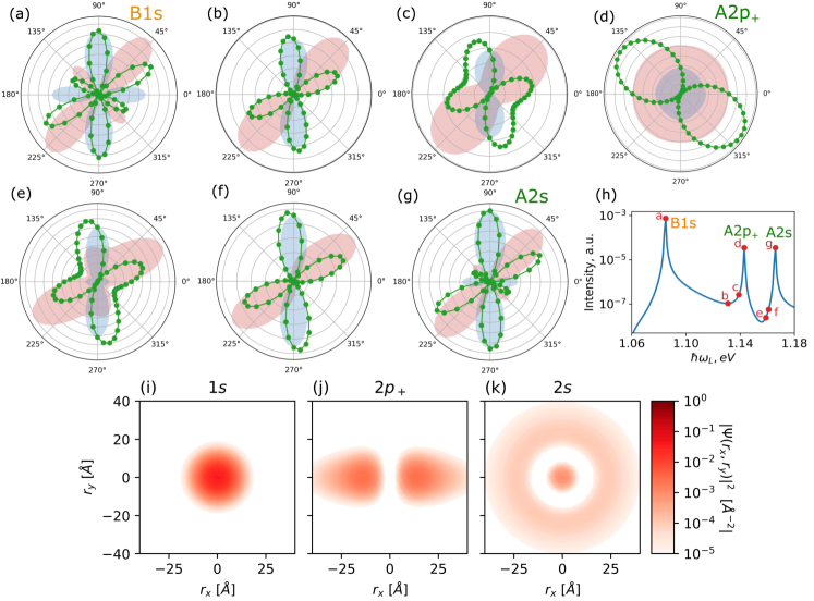
Figure 3: Angular dependence of $I$ and $|P_{x,y}|^{2}$ for the SHG in $\text{MoS}_{2}$ monolayer (a)-(g), calculated for driving field energies $\hbar\omega_{L}$ marked by the red points in the panel (h) [cf. Fig. 1c]. The driving amplitude is $f=0.1\rm\;\AA^{-1}$, which corresponds to laser intensity of $I\simeq 150$ GW/cm². Panels (i-k) show spatial profiles of the exciton wave amplitude $|\Psi|^{2}$ as a function of the electron-hole coordinate difference, calculated for excitonic states $1s$, $2p_{+}$, and $2s$.

III.2 Polarization diagrams

The SHG dependence on the polarization angle is illustrated in Fig. 2, which plots the angular dependence of $I_{2}(\phi)$: here, the value of $I_{2}$ is given by the radial distance from the diagram center. The resulting polarization diagrams, shown in Fig. 2, are calculated for a standalone $\text{MoS}_{2}$ monolayer for selected values of $f$ and three frequencies $\omega_{L}$, chosen to represent off-resonant excitation, the excitation at resonance with $A1s$ and $A2p_{+}$ states [see Fig. 1c]. The SHG intensity $I_{2}$ defined by Eq. (15) depends on polarization components, $|\bar{P}^{x}|$ and $|\bar{P}^{y}|$, that are also shown in Fig. 2 by the color shading. It is clearly seen that polarization diagrams are very sensitive to both the amplitude $f$ and frequency $\omega_{L}$ of the driving field.

In the linear response limit of $f\to 0$, the polarization diagram is circular in all cases (not shown). At the same time, at the very strong driving, it reveals a familiar symmetric six-leaf pattern. This pattern is defined by the single-particle dynamics that follows the crystal symmetry of $\text{MoS}_{2}$, and can be used to establish the orientation of the crystal lattice in experiments  Kumar et al. (2013); Malard et al. (2013); Li et al. (2013); Yin et al. (2014); Clark et al. (2014); Hsu et al. (2014). Exciton states start to play a much more significant role in the dynamics for the weaker driving, which is accompanied by drastic changes in the polarization diagram.

When the excitation is off-resonant and $f$ increases, the polarization diagram first develops a triangular shape, symmetric with respect to $120^{\circ}$ rotations. With the further increase in $f$, the angular dependence becomes, consecutively, first a three-leaf and then a six-leaf pattern. At still larger $f$, the six-leaf pattern becomes symmetric. Changes in the angular dependence of $I_{2}$ are accompanied by those in components $P^{x}$ and $P^{y}$, also shown in Fig. 2.

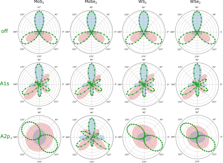
Figure 4: Angular dependence of the SHG intensity (green points) and polarization components $|P_{x}|^{2}$ (red shading) and $|P_{y}|^{2}$ (blue shading) for the driving amplitude $f=0.1\AA^{-1}$, calculated for monolayers $\text{MoS}_{2}$, $\text{MoSe}_{2}$, $\text{WS}_{2}$, and $\text{WSe}_{2}$ (panel columns) for the off-resonant driving with $\hbar\omega_{L}=0.35$eV (top row), at resonance with the $A1s$ state (middle row), and at resonance with the $A2p_{+}$ state (bottom row).

When the driving frequency is at resonance with an exciton state, the polarization diagram changes qualitatively depending on the exciton type. In the $A1s$ exciton resonance, the diagram develops an asymmetric six-leaf pattern already at very small amplitudes. The same six-leaf pattern remains for all values of $f$ becoming more symmetric at stronger driving.

In contrast, in the $A2p_{+}$ exciton resonance in Fig. 2, a six-leaf pattern is seen only at $f=0.25\AA^{-1}$, while at weaker driving, the diagram differs from both the off-resonant and the $A1s$ resonance cases. For a weaker driving with $f=10^{-3}\AA^{-1}$, the angular dependence has an asymmetric two-leaf shape. It becomes fully symmetric at larger amplitude $f=10^{-2}\AA^{-1}$. When $f$ increases, the butterfly-like pattern is formed with two equal side wings. With a further decrease in $f$, one observes four- and, then, six-leaf shapes.

Exciton-dependent differences in the polarization diagrams are further explored by tracing how the angular dependence changes with frequency $\omega_{L}$. Figure 3 illustrates the changes by showing a diagram sequence calculated for values of $\omega_{L}$ in the interval between $B1s$ and $A2s$ states (the calculations are done at $f=0.1\AA^{-1}$). When $\omega_{L}$ increases, a non-symmetric six-leaf shape, observed at the $B1s$ resonance, first changes into a four-leaf pattern, and then develops a butterfly-like shape with two wings, before transforming itself into a two-leaf pattern at the $A2p_{+}$ resonance. The $A2p_{-}$ resonance does not lead to resonant enhancement of the SHG signal, because of the absence of the dipole transition to the ground state Gong et al. (2017). With a further increase in $\omega_{L}$, these transformations take place in the reversed order, producing the original asymmetric six-leaf pattern when the $A2s$ resonance is reached.

One notes that the polarization diagrams observed at $A1s$, $B1s$ and $A2s$ resonances, shown in Figs. 2 and 3, have only marginal quantitative differences. This indicates that the SHG angular dependence is similar for excitonic states of the same spatial configurations. The angular dependence at different resonances is distinguishable only when excitons have different configuration. Spatial profiles of the exciton wave amplitude $|\Psi|^{2}$ for states $1s$, $2p_{+}$, and $2s$, as a function of the electron-hole coordinate difference ${\bf r}_{e}-{\bf r}_{h}$, are shown in Figs. 3i, j, and k, respectively. Figures 2 and 3 give a notable example of this dependence of the state symmetry: the angular diagram observed at the $A2p_{+}$ resonance deviates strongly from those at the $A1s$, $B1s$, and $A2s$ resonances. The same applies to the polarization components $P^{x,y}$ [see Fig. 3] implying that this conclusion holds for arbitrary measurements setup for SHG polarization.

III.3 Comparing different materials

We now compare SHG polarization diagrams for monolayers of $\text{MoS}_{2}$, $\text{MoSe}_{2}$, $\text{WS}_{2}$, and $\text{WSe}_{2}$. These materials have a qualitatively similar crystal configuration and, therefore, a similar band structure. One also identifies the same types of excitonic states, i.e., $s,p$, although their spectral positions differ. When the same states are identified, one calculates the corresponding SHG polarization diagrams.

In Fig. 4 the diagrams for these four materials calculated for the off-resonant driving, and the $A1s$ and $A2p_{+}$ resonances are plotted. One sees that the angular dependencies are indeed similar for all materials except for the $A2p_{+}$ resonance where $\text{MoSe}_{2}$ differs notably. The difference is explained by the fact that energies of the $A2p_{+}$ and $B1s$ states almost coincide in $\text{MoSe}_{2}$. This near degeneracy results in a mixture of signals typical for $B1s$ and $A2p_{+}$ resonances, which both contribute to the SHG and distort the angular dependence.

IV Discussion

A big variety of observed SHG polarization diagram types originate in the interplay of several factors affecting single- and two-particle states. Crystal symmetry is one of the factors defining SHG angular dependence. It is taken into account by the tridiagonal warping in the Dirac model for single-particle states. The warping violates the rotational symmetry, allowing additional optical transitions. This is illustrated in the inset in Fig. 1c, which shows a schematic structure of the low energy exciton states contributing most to the nonlinear dynamics. A rotational symmetry admits the transitions illustrated in this scheme by solid arrows. Optical transitions cannot connect any three-state sequence, making SHG forbidden in a rotationally invariant system, which can be formally shown, e.g., by solving the LvN equation perturbatively. The tridiagonal warping breaks the rotational symmetry allowing transitions between states $G$ and $2p_{+}$ (see Fig. 1). This creates four three-state sequences, $G\rightarrow 1s\rightarrow 2p_{+}$ and $G\rightarrow 2s\rightarrow 2p_{+}$, for $A$ and $B$ states, respectively, giving rise to SHG.

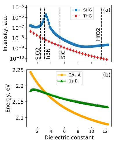
Figure 5: (a) Intensity of the second (blue squares) and third (red diamonds) harmonics on MoS₂ for the driving amplitude $f=0.1\AA^{-1}$ at resonance with the $A2p_{+}$ state as a function of the environment dielectric constant $\epsilon_{env}=(\epsilon_{1}+1)/2$, where $\epsilon_{1}$ is the static dielectric constant of the substrate. The dashed vertical lines correspond to $\epsilon_{env}$ values for the most commonly used substrates. (b) Energy of $B1s$ (green triangles) and $A2p_{+}$ excitons (yellow circles) as a function of the environment dielectric constant.

Another source of SHG is the quadratic term in the field-matter interaction Hamiltonian $H_{f}$, also introduced by the warping. The crystal symmetry is reflected in the matrix elements of $P^{\alpha}$ and $Q^{\alpha\beta}$ dipole operators entering $H_{f}$. There is a particular relation between these matrix elements and the SHG angular dependence, which can be illustrated by estimating the polarization vector components in $H_{f}$. Assuming symmetric transition matrix elements, one obtains a simple expression

$$P_{x}(\phi)=\tilde{f}\cos(\phi)-\alpha\tilde{f}^{2}\sin(2\phi),$$

$$P_{y}(\phi)=\tilde{f}\sin(\phi)-\alpha\tilde{f}^{2}\cos(2\phi),$$ (16)

where $\tilde{f}\propto f$. By substituting this polarization vector into Eq. (15) and assuming that $\alpha$ is a fitting parameter, one can quantitatively reproduce all the SHG angular dependencies for the off-resonant case in Fig. 2. When $\tilde{f}$ is small, the polarization is determined by the linear contribution, such that the SHG intensity is independent of the angle. In contrast, the larger driving field activates the quadratic contribution, which dominates the angular dependency of $I(\phi)$. In this case, a symmetric six-leaf pattern emerges, as shown in Fig. 2. In the regime of intermediate driving amplitude, the contributions of the linear and quadratic terms are comparable, and one observes a crossover between these two extreme regimes.

However, Eq. (16) can be used only for the case of the off-resonant excitation. At resonance with an excitonic state, the angular dependence becomes more complex due to a strong influence of the two-particle interactions. The configuration of an exciton state enables specific transition matrix elements, and this distorts the symmetry of the SHG angular dependence, as shown in Fig. 2 for $A1s$ and $A2p_{+}$ resonances. In addition, the Coulomb interaction enhances the dipole transitions and, hence, the linear term in Eq. (10).

Our results show that changes induced by the exciton-related effects are most notable at the $2p_{+}$-state resonances, where the linear term in Eq. (10) is dominant in a large interval of $f$ values. The crossover between the regimes of mostly linear and mostly quadratic contributions in the light-matter interaction $H_{f}$ takes place at $f_{c}\simeq 0.2\AA^{-1}$. This coincides with the upper applicability limit for the perturbation theory result $I\propto f^{4}$ in Fig. 1b. The stronger the driving, the larger is the quadratic contribution, and thus the closer to the symmetric six-leaf polarization diagram.

Another important aspect to consider is the role of the exciton mixing in different valleys. A well-established theoretical fact is that Coulomb exchange coupling for excitons in different valleys is proportional to the exciton momentum Qiu et al. (2015) and vanishes in the zero-momentum limit, considered here. At the same time, the existence of intervalley coupling in TMDCs is very well documented experimentally Yu et al. (2014); Hao et al. (2016). The strength of the intervalley coupling depends on many parameters such as doping Chakraborty et al. (2019), dielectric environment Paradisanos et al. (2020), magnetic field Wang et al. (2016), and strength of disorder Wang et al. (2013). Besides the Coulomb exchange interaction (at finite momentum), other mechanisms such as the electron-phonon and short-range disorder interactions could lead to the intervalley coupling, and there are ongoing debates as to which of those is the dominant one Yu and Wu (2014); Glazov et al. (2014); Schaibley et al. (2016); Glazov et al. (2017); Paradisanos et al. (2020). Since we deal with doubly degenerate states, the interaction between them of any infinitesimal strength would mix the wavefunctions of those states by 50%, even though the energies of those states would not change much. We performed controlled calculations, where doubly degenerate states originating from different valleys are mixed by 50%, i.e., $\Psi_{new1}=(\Psi_{old1}+\Psi_{old2})/\sqrt{2}$, $\Psi_{new2}=(\Psi_{old1}-\Psi_{old2})/\sqrt{2}$, where old and new subscripts refer to the old and new wavefunctions, correspondingly. When the matrix elements entering the Hamiltonian for the Liouville - von Neumann equation use new wavefunctions, we do not find changes in the resulting angular polarization diagrams reported earlier. Therefore, our main conclusions on the angular polarization diagram dependence on the excitation power and resonant conditions are not sensitive to the $K-K’$ valley exciton mixing.

Finally, we discuss the influence of the dielectric environment on the excitonic effects in the nonlinear response. The environment affects the effective dielectric constant of the system, modifying the strength of the Coulomb interaction, the binding energy of excitons, and, thus, their contribution to the dynamics. This is illustrated in Fig. 5a, which plots the intensity of the second and third harmonics at resonance with the $A2p_{+}$ state as functions of the environment dielectric constant $\epsilon_{env}$. As $\epsilon_{env}$ increases from 1 to 10, the intensity of both harmonics decreases by more than two orders of magnitude. A sharp peak in the SHG signal at $\epsilon_{env}\simeq 4$ in Fig. 5a appears due to the degeneracy of the $A2p_{+}$ and $B1s$ energies at this point [see Fig. 5b].

In order to observe the polarization pattern change, the field amplitude has to be reduced by an order of magnitude under off-resonant conditions (see the top panels in Fig. 2), which in turn translates into a four-orders-of-magnitude reduction in the SHG signal (see Fig. 1b). This creates a tremendous challenge in the experiment to observe an ultra-low SHG signal. A much more favorable situation occurs when the excitation laser energy resonates with half the energy of the $A2p_{+}$ exciton (see the bottom panels in Fig. 2). In this case, a reduction of a factor of two in field amplitude or only one order of magnitude in laser intensity is needed to observe substantial changes in the polarization pattern. Since the exciton energies are sensitive to doping and the dielectric environment, the most favorable measurement setup would involve scanning the excitation laser wavelength at fixed laser power. According to Fig. 3, a six-leaf pattern would evolve into a four-leaf pattern and a two-leaf pattern under a realistic laser intensity of about 150 GW/cm². Thermal management can be improved by choosing dielectric substrates with high thermal conductivity, such as diamond, to avoid sample burning. However, suspended samples can enable measurements in the transmission mode with the use of two different polarizers for the excitation laser energy and its second harmonic overturn. According to Fig. 5a, a reduced dielectric screening of the environment gives a two-orders-of-magnitude enhancement of the SHG signal, which significantly reduces the length of time of measurements that is needed for a good signal-to-noise ratio.

V Conclusions

Our work demonstrates that SHG in TMDC monolayers is notably affected by the many-particle exciton effects. The SHG signal increases by orders of magnitude when the driving pulse is at resonance with an excitonic state. More importantly, excitons alter the SHG polarization angular dependence qualitatively. Its dependence on the energy and amplitude of the driving field undergoes significant changes depending on the type of the resonating exciton. The influence of excitons gives rise to deviations from the symmetric six-leaf angular dependence in monolayers with an undistorted crystal structure. This conclusion is generic, being supported by the qualitatively similar polarization patterns and their changes obtained for $\text{MoS}_{2}$, $\text{MoSe}_{2}$, $\text{WS}_{2}$, and $\text{WSe}_{2}$.

Our results open a pathway to a nonlinear spectroscopy method to probe exciton states by the symmetry of the polarization angular dependence of the SHG signal measured as a function of the excitation strength. Indeed, nonlinear spectroscopy can probe Rydberg states of strongly bound excitons in a one-dimensional system Wang et al. (2005); Maultzsch et al. (2005), not accessible in linear optical absorption. Two-dimensional materials offer a rich diversity of optical signatures in photoluminescence spectra Wang et al. (2018); the origin of some of them is still not identified. The SHG polarization angular dependence as a function of excitation power offers a powerful characterization tool to unravel the nature of strongly correlated excited states in low-dimensional materials in addition to the commonly used magnetic-field- and electric-field-dependent optical spectroscopy.

References

- Boyd (2020) R. W. Boyd, Nonlinear Optics (Academic Press, New York, USA, 2020).
- Ghimire et al. (2010) S. Ghimire, A. D. DiChiara, E. Sistrunk, P. Agostini, L. F. DiMauro, and D. A. Reis, Observation of high-order harmonic generation in a bulk crystal, Nature Physics 7, 138 (2010).
- Chin et al. (2001) A. H. Chin, O. G. Calderón, and J. Kono, Extreme midinfrared nonlinear optics in semiconductors, Physical Review Letters 86, 3292 (2001).
- Belyanin et al. (2005) A. Belyanin, F. Xie, D. Liu, F. Capasso, and M. Troccoli, Coherent nonlinear optics with quantum cascade structures, Journal of Modern Optics 52, 2293 (2005).
- Prasad and Williams (1991) P. N. Prasad and D. J. Williams, Introduction to Nonlinear Optical Effects in Molecules and Polymers (Wiley-Interscience, New York, USA, 1991).
- Dominicis et al. (2004) L. D. Dominicis, S. Botti, L. S. Asilyan, R. Ciardi, R. Fantoni, M. L. Terranova, A. Fiori, S. Orlanducci, and R. Appolloni, Second- and third- harmonic generation in single-walled carbon nanotubes at nanosecond time scale, Applied Physics Letters 85, 1418 (2004).
- Murakami and Kono (2009) Y. Murakami and J. Kono, Nonlinear photoluminescence excitation spectroscopy of carbon nanotubes: Exploring the upper density limit of one-dimensional excitons, Physical Review Letters 102, 037401 (2009).
- Kono (2013) J. Kono, Ultrafast and nonlinear optics in carbon nanomaterials, Journal of Physics: Condensed Matter 25, 050301 (2013).
- Kumar et al. (2013) N. Kumar, S. Najmaei, Q. Cui, F. Ceballos, P. M. Ajayan, J. Lou, and H. Zhao, Second harmonic microscopy of monolayer MoS2, Physical Review B 87, 161403(R) (2013).
- Malard et al. (2013) L. M. Malard, T. V. Alencar, A. P. M. Barboza, K. F. Mak, and A. M. de Paula, Observation of intense second harmonic generation from MoS2 atomic crystals, Physical Review B 87, 201401(R) (2013).
- Yin et al. (2014) X. Yin, Z. Ye, D. A. Chenet, Y. Ye, K. O'Brien, J. C. Hone, and X. Zhang, Edge nonlinear optics on a MoS2 atomic monolayer, Science 344, 488 (2014).
- Clark et al. (2014) D. J. Clark, V. Senthilkumar, C. T. Le, D. L. Weerawarne, B. Shim, J. I. Jang, J. H. Shim, J. Cho, Y. Sim, M.-J. Seong, S. H. Rhim, A. J. Freeman, K.-H. Chung, and Y. S. Kim, Strong optical nonlinearity of CVD-grown MoS2 monolayer as probed by wavelength-dependent second-harmonic generation, Physical Review B 90, 121409(R) (2014).
- Hsu et al. (2014) W.-T. Hsu, Z.-A. Zhao, L.-J. Li, C.-H. Chen, M.-H. Chiu, P.-S. Chang, Y.-C. Chou, and W.-H. Chang, Second harmonic generation from artificially stacked transition metal dichalcogenide twisted bilayers, ACS Nano 8, 2951 (2014).
- Janisch et al. (2014) C. Janisch, Y. Wang, D. Ma, N. Mehta, A. L. Elías, N. Perea-López, M. Terrones, V. Crespi, and Z. Liu, Extraordinary second harmonic generation in tungsten disulfide monolayers, Scientific Reports 4, 5530 (2014).
- Jiang et al. (2014) T. Jiang, H. Liu, D. Huang, S. Zhang, Y. Li, X. Gong, Y.-R. Shen, W.-T. Liu, and S. Wu, Valley and band structure engineering of folded MoS2 bilayers, Nature Nanotechnology 9, 825 (2014).
- Liu et al. (2016) H. Liu, Y. Li, Y. S. You, S. Ghimire, T. F. Heinz, and D. A. Reis, High-harmonic generation from an atomically thin semiconductor, Nature Physics 13, 262 (2016).
- Säynätjoki et al. (2017) A. Säynätjoki, L. Karvonen, H. Rostami, A. Autere, S. Mehravar, A. Lombardo, R. A. Norwood, T. Hasan, N. Peyghambarian, H. Lipsanen, K. Kieu, A. C. Ferrari, M. Polini, and Z. Sun, Ultra-strong nonlinear optical processes and trigonal warping in MoS2 layers, Nature Communications 8, 893 (2017).
- Autere et al. (2018) A. Autere, H. Jussila, Y. Dai, Y. Wang, H. Lipsanen, and Z. Sun, Nonlinear optics with 2d layered materials, Advanced Materials 30, 1705963 (2018).
- Mennel et al. (2018) L. Mennel, M. M. Furchi, S. Wachter, M. Paur, D. K. Polyushkin, and T. Mueller, Optical imaging of strain in two-dimensional crystals, Nature Communications 9, 516 (2018).
- Mennel et al. (2019) L. Mennel, M. Paur, and T. Mueller, Second harmonic generation in strained transition metal dichalcogenide monolayers: MoS2, MoSe2, WS2, and WSe2, APL Photonics 4, 034404 (2019).
- Stiehm et al. (2019) T. Stiehm, R. Schneider, J. Kern, I. Niehues, S. M. de Vasconcellos, and R. Bratschitsch, Supercontinuum second harmonic generation spectroscopy of atomically thin semiconductors, Review of Scientific Instruments 90, 083102 (2019).
- Maragkakis et al. (2019) G. M. Maragkakis, , S. Psilodimitrakopoulos, L. Mouchliadis, I. Paradisanos, A. Lemonis, G. Kioseoglou, E. Stratakis, and and, Imaging the crystal orientation of 2d transition metal dichalcogenides using polarization-resolved second-harmonic generation, Opto-Electronic Advances 2, 19002601 (2019).
- Lin et al. (2019) K.-Q. Lin, S. Bange, and J. M. Lupton, Quantum interference in second-harmonic generation from monolayer WSe2, Nature Physics 15, 242 (2019).
- Zhang et al. (2020) J. Zhang, W. Zhao, P. Yu, G. Yang, and Z. Liu, Second harmonic generation in 2d layered materials, 2D Materials 7, 042002 (2020).
- Khan et al. (2020) A. R. Khan, B. Liu, T. Lü, L. Zhang, A. Sharma, Y. Zhu, W. Ma, and Y. Lu, Direct measurement of folding angle and strain vector in atomically thin WS2 using second-harmonic generation, ACS Nano 14, 15806 (2020).
- Ho et al. (2020) Y. W. Ho, H. G. Rosa, I. Verzhbitskiy, M. J. L. F. Rodrigues, T. Taniguchi, K. Watanabe, G. Eda, V. M. Pereira, and J. C. Viana-Gomes, Measuring valley polarization in two-dimensional materials with second-harmonic spectroscopy, ACS Photonics 7, 925 (2020).
- Heinz (1991) T. Heinz, in Modern Problems in Condensed Matter Sciences, Vol. 29 (Elsevier, Amsterdam, 1991) Chap. 5, pp. 353–416.
- Fiebig et al. (1998) M. Fiebig, D. Fröhlich, S. Leute, and R. V. Pisarev, Second harmonic spectroscopy and control of domain size in antiferromagnetic YMnO3, Journal of Applied Physics 83, 6560 (1998).
- Shree et al. (2020) S. Shree, I. Paradisanos, X. Marie, C. Robert, and B. Urbaszek, Guide to optical spectroscopy of layered semiconductors, Nature Reviews Physics 3, 39 (2020).
- Fiebig et al. (2005) M. Fiebig, V. V. Pavlov, and R. V. Pisarev, Second-harmonic generation as a tool for studying electronic and magnetic structures of crystals: review, Journal of the Optical Society of America B 22, 96 (2005).
- Ma et al. (2020) H. Ma, J. Liang, H. Hong, K. Liu, D. Zou, M. Wu, and K. Liu, Rich information on 2d materials revealed by optical second harmonic generation, Nanoscale 12, 22891 (2020).
- Li et al. (2013) Y. Li, Y. Rao, K. F. Mak, Y. You, S. Wang, C. R. Dean, and T. F. Heinz, Probing symmetry properties of few-layer MoS2 and h-BN by optical second-harmonic generation, Nano Letters 13, 3329 (2013).
- Yu et al. (2016) R. Yu, J. D. Cox, and F. J. G. de Abajo, Nonlinear plasmonic sensing with nanographene, Physical Review Letters 117, 123904 (2016).
- Wehling et al. (2015) T. O. Wehling, A. Huber, A. I. Lichtenstein, and M. I. Katsnelson, Probing of valley polarization in graphene via optical second-harmonic generation, Physical Review B 91, 041404(R) (2015).
- Hipolito and Pereira (2017) F. Hipolito and V. M. Pereira, Second harmonic spectroscopy to optically detect valley polarization in 2d materials, 2D Materials 4, 021027 (2017).
- Zhou et al. (2015) X. Zhou, J. Cheng, Y. Zhou, T. Cao, H. Hong, Z. Liao, S. Wu, H. Peng, K. Liu, and D. Yu, Strong second-harmonic generation in atomic layered GaSe, Journal of the American Chemical Society 137, 7994 (2015).
- Mak et al. (2010) K. F. Mak, C. Lee, J. Hone, J. Shan, and T. F. Heinz, Atomically thin : A new direct-gap semiconductor, Phys. Rev. Lett. 105, 136805 (2010).
- Splendiani et al. (2010) A. Splendiani, L. Sun, Y. Zhang, T. Li, J. Kim, C.-Y. Chim, G. Galli, and F. Wang, Emerging photoluminescence in monolayer mos2, Nano Letters 10, 1271 (2010).
- Chernikov et al. (2014) A. Chernikov, T. C. Berkelbach, H. M. Hill, A. Rigosi, Y. Li, O. B. Aslan, D. R. Reichman, M. S. Hybertsen, and T. F. Heinz, Exciton binding energy and nonhydrogenic rydberg series in MonolayerWS2, Physical Review Letters 113, 076802 (2014).
- Seyler et al. (2015) K. L. Seyler, J. R. Schaibley, P. Gong, P. Rivera, A. M. Jones, S. Wu, J. Yan, D. G. Mandrus, W. Yao, and X. Xu, Electrical control of second-harmonic generation in a WSe2 monolayer transistor, Nature Nanotechnology 10, 407 (2015).
- Wang et al. (2015) G. Wang, X. Marie, I. Gerber, T. Amand, D. Lagarde, L. Bouet, M. Vidal, A. Balocchi, and B. Urbaszek, Giant enhancement of the optical second-harmonic emission ofWSe2monolayers by laser excitation at exciton resonances, Physical Review Letters 114, 097403 (2015).
- Wang et al. (2018) G. Wang, A. Chernikov, M. M. Glazov, T. F. Heinz, X. Marie, T. Amand, and B. Urbaszek, Colloquium : Excitons in atomically thin transition metal dichalcogenides, Reviews of Modern Physics 90, 021001 (2018).
- Cheiwchanchamnangij and Lambrecht (2012) T. Cheiwchanchamnangij and W. R. L. Lambrecht, Quasiparticle band structure calculation of monolayer, bilayer, and bulk mos2, Phys. Rev. B 85, 205302 (2012).
- Ramasubramaniam (2012) A. Ramasubramaniam, Large excitonic effects in monolayers of molybdenum and tungsten dichalcogenides, Phys. Rev. B 86, 115409 (2012).
- Qiu et al. (2013) D. Y. Qiu, F. H. da Jornada, and S. G. Louie, Optical spectrum of : Many-body effects and diversity of exciton states, Phys. Rev. Lett. 111, 216805 (2013).
- Berkelbach et al. (2013) T. C. Berkelbach, M. S. Hybertsen, and D. R. Reichman, Theory of neutral and charged excitons in monolayer transition metal dichalcogenides, Phys. Rev. B 88, 045318 (2013).
- Qiu et al. (2015) D. Y. Qiu, T. Cao, and S. G. Louie, Nonanalyticity, valley quantum phases, and lightlike exciton dispersion in monolayer transition metal dichalcogenides: Theory and first-principles calculations, Phys. Rev. Lett. 115, 176801 (2015).
- Zhumagulov et al. (2020a) Y. V. Zhumagulov, A. Vagov, N. Y. Senkevich, D. R. Gulevich, and V. Perebeinos, Three-particle states and brightening of intervalley excitons in a doped MoS2 monolayer, Physical Review B 101, 245433 (2020a).
- Zhumagulov et al. (2020b) Y. V. Zhumagulov, A. Vagov, D. R. Gulevich, P. E. Faria Junior, and V. Perebeinos, Trion induced photoluminescence of a doped MoS2 monolayer, The Journal of Chemical Physics 153, 044132 (2020b).
- Zhumagulov et al. (2021) Y. V. Zhumagulov, A. Vagov, D. R. Gulevich, and V. Perebeinos, Electrostatic control of the trion fine structure in transition metal dichalcogenide monolayers (2021), arXiv:2104.11800 .
- Trolle et al. (2014) M. L. Trolle, G. Seifert, and T. G. Pedersen, Theory of excitonic second-harmonic generation in monolayerMoS2, Physical Review B 89, 235410 (2014).
- Grüning and Attaccalite (2014) M. Grüning and C. Attaccalite, Second harmonic generation inh-BN and MoS2monolayers: Role of electron-hole interaction, Physical Review B 89, 081102(R) (2014).
- Glazov et al. (2017) M. M. Glazov, L. E. Golub, G. Wang, X. Marie, T. Amand, and B. Urbaszek, Intrinsic exciton-state mixing and nonlinear optical properties in transition metal dichalcogenide monolayers, Physical Review B 95, 035311 (2017).
- Kolos et al. (2021) M. Kolos, L. Cigarini, R. Verma, F. Karlický, and S. Bhattacharya, Giant linear and nonlinear excitonic responses in an atomically thin indirect semiconductor nitrogen phosphide, The Journal of Physical Chemistry C 125, 12738 (2021).
- Richter and Knorr (2010) M. Richter and A. Knorr, A time convolution less density matrix approach to the nonlinear optical response of a coupled system–bath complex, Annals of Physics 325, 711 (2010).
- Axt and Kuhn (2004) V. M. Axt and T. Kuhn, Femtosecond spectroscopy in semiconductors: a key to coherences, correlations and quantum kinetics, Reports on Progress in Physics 67, 433 (2004).
- Xiao et al. (2012) D. Xiao, G.-B. Liu, W. Feng, X. Xu, and W. Yao, Coupled spin and valley physics in monolayers of MoS2 and other group-VI dichalcogenides, Phys. Rev. Lett. 108, 196802 (2012).
- Kormányos et al. (2013) A. Kormányos, V. Zólyomi, N. D. Drummond, P. Rakyta, G. Burkard, and V. I. Fal'ko, Monolayer MoS2: Trigonal warping, the gamma valley, and spin-orbit coupling effects, Physical Review B 88, 045416 (2013).
- Kormányos et al. (2015) A. Kormányos, G. Burkard, M. Gmitra, J. Fabian, V. Zólyomi, N. D. Drummond, and V. Fal’ko, kptheory for two-dimensional transition metal dichalcogenide semiconductors, 2D Mater. 2, 022001 (2015).
- Taghizadeh and Pedersen (2019) A. Taghizadeh and T. G. Pedersen, Nonlinear optical selection rules of excitons in monolayer transition metal dichalcogenides, Physical Review B 99, 235433 (2019).
- Cho and Berkelbach (2018) Y. Cho and T. C. Berkelbach, Environmentally sensitive theory of electronic and optical transitions in atomically thin semiconductors, Phys. Rev. B 97, 041409(R) (2018).
- Zollner et al. (2019) K. Zollner, P. E. Faria Junior, and J. Fabian, Strain-tunable orbital, spin-orbit, and optical properties of monolayer transition-metal dichalcogenides, Phys. Rev. B 100, 195126 (2019).
- Laturia et al. (2018) A. Laturia, M. L. V. de Put, and W. G. Vandenberghe, Dielectric properties of hexagonal boron nitride and transition metal dichalcogenides: from monolayer to bulk, npj 2D Materials and Applications 2, 6 (2018).
- Zhang et al. (2016) C. Zhang, C. Gong, Y. Nie, K.-A. Min, C. Liang, Y. J. Oh, H. Zhang, W. Wang, S. Hong, L. Colombo, R. M. Wallace, and K. Cho, Systematic study of electronic structure and band alignment of monolayer transition metal dichalcogenides in van der waals heterostructures, 2D Materials 4, 015026 (2016).
- Sipe and Ghahramani (1993) J. E. Sipe and E. Ghahramani, Nonlinear optical response of semiconductors in the independent-particle approximation, Phys. Rev. B 48, 11705 (1993).
- Rohlfing and Louie (2000) M. Rohlfing and S. G. Louie, Electron-hole excitations and optical spectra from first principles, Phys. Rev. B 62, 4927 (2000).
- Rytova (1967) N. S. Rytova, The screened potential of a point charge in a thin film, Moscow University Physics Bulletin 3, 18 (1967).
- Keldysh (1979) L. V. Keldysh, Coulomb interaction in thin semiconductor and semimetal films, Soviet Journal of Experimental and Theoretical Physics Letters 29, 658 (1979).
- Sipe and Shkrebtii (2000) J. E. Sipe and A. I. Shkrebtii, Second-order optical response in semiconductors, Phys. Rev. B 61, 5337 (2000).
- Johansson et al. (2012) J. Johansson, P. Nation, and F. Nori, QuTiP: An open-source python framework for the dynamics of open quantum systems, Computer Physics Communications 183, 1760 (2012).
- Johansson et al. (2013) J. Johansson, P. Nation, and F. Nori, QuTiP 2: A python framework for the dynamics of open quantum systems, Computer Physics Communications 184, 1234 (2013).
- Gong et al. (2017) P. Gong, H. Yu, Y. Wang, and W. Yao, Optical selection rules for excitonic rydberg series in the massive dirac cones of hexagonal two-dimensional materials, Phys. Rev. B 95, 125420 (2017).
- Yu et al. (2014) H. Yu, G.-B. Liu, P. Gong, X. Xu, and W. Yao, Dirac cones and dirac saddle points of bright excitons in monolayer transition metal dichalcogenides, Nature Communications 5, 3876 (2014).
- Hao et al. (2016) K. Hao, G. Moody, F. Wu, C. K. Dass, L. Xu, C.-H. Chen, L. Sun, M.-Y. Li, L.-J. Li, A. H. MacDonald, and X. Li, Direct measurement of exciton valley coherence in monolayer wse2, Nature Physics 12, 677 (2016).
- Chakraborty et al. (2019) C. Chakraborty, A. Mukherjee, L. Qiu, and A. N. Vamivakas, Electrically tunable valley polarization and valley coherence in monolayer wse2 embedded in a van der waals heterostructure, Opt. Mater. Express 9, 1479 (2019).
- Paradisanos et al. (2020) I. Paradisanos, K. M. McCreary, D. Adinehloo, L. Mouchliadis, J. T. Robinson, H.-J. Chuang, A. T. Hanbicki, V. Perebeinos, B. T. Jonker, E. Stratakis, and G. Kioseoglou, Prominent room temperature valley polarization in ws2/graphene heterostructures grown by chemical vapor deposition, Applied Physics Letters 116, 203102 (2020).
- Wang et al. (2016) G. Wang, X. Marie, B. L. Liu, T. Amand, C. Robert, F. Cadiz, P. Renucci, and B. Urbaszek, Control of exciton valley coherence in transition metal dichalcogenide monolayers, Phys. Rev. Lett. 117, 187401 (2016).
- Wang et al. (2013) Q. Wang, S. Ge, X. Li, J. Qiu, Y. Ji, J. Feng, and D. Sun, Valley carrier dynamics in monolayer molybdenum disulfide from helicity-resolved ultrafast pump–probe spectroscopy, ACS Nano 7, 11087 (2013).
- Yu and Wu (2014) T. Yu and M. W. Wu, Valley depolarization due to intervalley and intravalley electron-hole exchange interactions in monolayer , Phys. Rev. B 89, 205303 (2014).
- Glazov et al. (2014) M. M. Glazov, T. Amand, X. Marie, D. Lagarde, L. Bouet, and B. Urbaszek, Exciton fine structure and spin decoherence in monolayers of transition metal dichalcogenides, Phys. Rev. B 89, 201302(R) (2014).
- Schaibley et al. (2016) J. R. Schaibley, H. Yu, G. Clark, P. Rivera, J. S. Ross, K. L. Seyler, W. Yao, and X. Xu, Valleytronics in 2d materials, Nature Reviews Materials 1, 16055 (2016).
- Wang et al. (2005) F. Wang, G. Dukovic, L. E. Brus, and T. F. Heinz, The optical resonances in carbon nanotubes arise from excitons, Science 308, 838 (2005).
- Maultzsch et al. (2005) J. Maultzsch, R. Pomraenke, S. Reich, E. Chang, D. Prezzi, A. Ruini, E. Molinari, M. S. Strano, C. Thomsen, and C. Lienau, Exciton binding energies in carbon nanotubes from two-photon photoluminescence, Phys. Rev. B 72, 241402(R) (2005).