Cooling Improves Cosmic Microwave Background Map-Making When Low-Frequency Noise is Large

Abstract

In the context of Cosmic Microwave Background data analysis, we study the solution to the equation that transforms scanning data into a map. As originally suggested in “messenger” methods for solving linear systems, we split the noise covariance into uniform and non-uniform parts and adjust their relative weights during the iterative solution. With simulations, we study mock instrumental data with different noise properties, and find that this “cooling” or perturbative approach is particularly effective when there is significant low-frequency noise in the timestream. In such cases, a conjugate gradient algorithm applied to this modified system converges faster and to a higher fidelity solution than the standard conjugate gradient approach. We give an analytic estimate for the parameter that controls how gradually the linear system should change during the course of the solution.

1 Introduction

In observations of the Cosmic Microwave Background (CMB), map-making is an intermediate step between the collection of raw scanning data and the scientific analyses, such as the estimation of power spectra and cosmological parameters. Next generation CMB observations will generate much more data than those today, and so it is worth exploring efficient ways to process the data even though, on paper, the map-making problem has long been solved.

The time-ordered scanning data is summarized by

$$\mathbf{d}=P\mathbf{m}+\mathbf{n}$$ (1)

where $\mathbf{d}$, $\mathbf{m}$, and $\mathbf{n}$ are the vectors of time-ordered data (TOD), the CMB sky-map signal, and measurement noise. $P$ is a sparse matrix in the time-by-pixel domain that encodes the telescope’s pointing. Of several map-making methods (Tegmark, 1997), one of the most common is the method introduced for the Cosmic Background Explorer (COBE, Janssen & Gulkis, 1992). This optimal, linear solution is

$$\quantity(P^{\dagger}N^{-1}P)\mathbf{\hat{m}}=P^{\dagger}N^{-1}\mathbf{d}$$ (2)

where $\mathbf{\hat{m}}$ provides the standard generalized least squares minimization of the $\chi^{2}$ statistic,

$$\chi^{2}(\mathbf{m}) \equiv(\mathbf{d}-P\mathbf{m})^{\dagger}N^{-1}(\mathbf{d}-P\mathbf{m}).$$ (3)

Here we assume that the noise has zero mean $\expectationvalue{\mathbf{n}}=\mathbf{0}$, and the noise covariance matrix $N=\expectationvalue{\mathbf{n}\mathbf{n}^{\dagger}}$ is diagonal in frequency space. In the case where the noise is Gaussian, the COBE solution is also the maximum likelihood solution.

With current computational power, we cannot solve for $\mathbf{\hat{m}}$ by calculating $\quantity(P^{\dagger}N^{-1}P)^{-1}P^{\dagger}N^{-1}\mathbf{d}$ directly. The noise covariance matrix $N$ is often sparse in the frequency domain and the pointing matrix $P$ is sparse in the time-by-pixel domain. In experiments currently under design, there may be $\sim 10^{16}$ time samples and $\sim 10^{9}$ pixels, so these matrix inversions are intractable unless the covariance is uniform (proportional to the identity matrix $I$). We can use iterative methods, such as conjugate gradient descent, to avoid the matrix inversions, and execute each matrix multiplication in a basis where the matrix is sparse, using a fast Fourier transform to go between the frequency and time domain.

As an alternative to conjugate gradient descent, Huffenberger & Næss (2018) showed that the “messenger” iterative method could be adapted to solve the linear map-making system, based on the approach from Elsner & Wandelt (2013) to solve the linear Wiener filter. This technique splits the noise covariance into a uniform part and the remainder, and introduces an additional vector that represent the signal plus uniform noise. This messenger field acts as an intermediary between the signal and the data and has a covariance that is conveniently sparse in every basis. Elsner & Wandelt (2013) also introduced a cooling scheme that takes advantage of the split covariance: over the course of the iterative solution, we adjust the relative weight of those two parts. Starting with the uniform covariance, the modified linear system gradually transforms to the final system, under the control of a cooling parameter. In numerical experiments, Huffenberger & Næss (2018) found that a map produced by the cooled messenger method converged significantly faster than for standard conjugate gradient methods, and to higher fidelity, especially on large scales.

Papež et al. (2018) showed that the the messenger field approach is equivalent to a fixed point iteration scheme, and studied its convergence properties in detail. Furthermore, they showed that the split covariance and the modified system that incorporates the cooling can be solved by other means, including a conjugate gradient technique, which should generally show better convergence properties than the fixed-point scheme. With simulations, we have confirmed this conclusion. In their numerical tests, Papež et al. (2018) did not find benefits to the cooling modification of the map-making system, in contrast to the findings of Huffenberger & Næss (2018).

In this paper, we show that the difference arose because the numerical tests in Papež et al. (2018) used much less low-frequency (or $1/f$) noise than Huffenberger & Næss (2018), and show that the cooling technique improves map-making performance especially when the low-frequency noise is large. This performance boost depends on a proper choice for the pace of cooling. Kodi Ramanah et al. (2017) showed that for Wiener filter the cooling parameter should be chosen as a geometric series. In this work, we give an alternative interpretation of the parameterizing process and show that for map-making the optimal choice (unsurprisingly) is also a geometric series.

In Section 2 we describe our methods for treating the map-making equation and our numerical experiments. In Section 3 we present our results. In Section 4, we list our conclusions. In Appendix A we derive the prescription for our cooling schedule.

2 Methods

2.1 Parameterized Conjugate Gradient Method

The messenger field approach introduced an extra cooling parameter $\lambda$ to the map-making equation, and solved the linear system with an alternative parameterized covariance $N(\lambda)=\lambda\tau I+\bar{N}$. The parameter $\tau=\min(\operatorname*{diag}(N))$ represents the uniform level of (white) noise in the original covariance. The remainder $\bar{N}\equiv N-\tau I$ is the non-uniform part of the original noise covariance. (Here $N$ without any arguments denotes the original noise covariance matrix $N=\expectationvalue{\mathbf{n}\mathbf{n}^{\dagger}}$.) In this work we find it more convenient to work with the reciprocal of cooling parameter $\eta=\lambda^{-1}$ which represents the degree of heteroscedasticity (non-uniformity) in the parameterized covariance

$$N(\eta)=\tau I+\eta\bar{N}.$$ (4)

When $\eta=1$ this parameterized covariance $N(\eta)$ equals $N$.

Papež et al. (2018) showed that the conjugate gradient method can be easily applied to the cooled map-making problem. In our notation, this is equivalent to iterating on the parameterized map-making equation

$$\quantity(P^{\dagger}N(\eta_{i})^{-1}P)\,\mathbf{\hat{m}}(\eta_{i})=P^{\dagger}N(\eta_{i})^{-1}\mathbf{d},$$ (5)

as we adjust the parameter through a set of levels $\{\eta_{i}\}$. (We use $\mathbf{\hat{m}}$ with no $\eta$ argument to mean the estimated $\mathbf{\hat{m}}$ in Eq. 2, independent of $\eta$.) This equation leads to the same system as the paramaterized equation in the messenger field method, because $N(\eta)=\lambda^{-1}N(\lambda)$ and the condition number do not change upon scalar multiplication to both sides of the equation. For concreteness we fix the preconditioner to $M=P^{\dagger}P$ for all calculations.

When $\eta=0$, the noise covariance matrix $N(0)$ is homoscedastic (uniform), and the solution is given by the simple binned map $\mathbf{\hat{m}}(0)=\quantity(P^{\dagger}P)^{-1}P^{\dagger}\mathbf{d}$, which can be solved directly.

Since the non-white part $\bar{N}$ is the troublesome portion of the covariance, we can think of the $\eta$ parameter as increasing the heteroscedasticity of the system, adding a perturbation to the solution achieved at a particular stage, building ultimately upon the initial uniform covariance model. Therefore, this quasi-static process requires $\eta$ increase as $0=\eta_{0}\leq\eta_{1}\leq\cdots\leq\eta_{\rm final}=1$, at which point we arrive at the desired map-making equation, and the solution $\mathbf{\hat{m}}(1)=\mathbf{\hat{m}}$.

We may iterate more than once at each intermediate $\eta_{i}$: we solve equation (5) with conjugate gradient iterations using the result from the previous calculation $\mathbf{\hat{m}}(\eta_{i-1})$ as the initial value. We move to next parameter $\eta_{i+1}$ when the norm of residual vector

$$\norm{\mathbf{r}(\mathbf{m},\eta_{i})}\equiv\norm{P^{\dagger}N(\eta_{i})^{-1}P\,\mathbf{m}-P^{\dagger}N(\eta_{i})^{-1}\mathbf{d}}$$ (6)

is an order of magnitude smaller than the norm of the right hand side of Eq. 5.

$$\norm{\mathbf{r}(\mathbf{m},\eta_{i})}<0.1\ \norm{P^{\dagger}N(\eta_{i})^{-1}\mathbf{d}}$$ (7)

This is not stringent enough to completely converge at this $\eta$-level, but we find that it causes the system to converge sufficiently to allow us to move on to the next $\eta$.

2.2 Analytical expression for $\quantity{\eta_{i}}$ series

The next question is how to appropriately choose these monotonically increasing parameters $\eta$. We also want to determine $\eta_{1},\cdots,\eta_{n-1}$ before starting conjugate gradient iterations, because the time ordered data $\mathbf{d}$ is very large, and we do not want to keep it in the system memory during calculation or repeatedly read it in from disk. If we determine $\eta_{1},\cdots,\eta_{n-1}$ before the iterations, then we can precompute the right-hand side of Eq. 5 for each $\eta_{i}$ and keep these map-sized objects, instead of the entire time-ordered data.

In Appendix A, we show that a generic good choice for the $\eta$ parameters is given by this geometric series

$$\eta_{i}=\min\quantity\bigg{\quantity(2^{i}-1)\frac{\tau}{\max(\bar{N}_{f})},\;1},$$ (8)

where $\bar{N}_{f}$ are the eigenvalues of $\bar{N}$ under frequency representation. This is one of our main results. It not only tells us how to choose parameters $\eta_{i}$, but also when we should stop the perturbation, and set $\eta=1$. For example, if the noise covariance matrix $N$ is almost uniform, then $\bar{N}=N-\tau I\approx 0$, and we would have ${\tau}/{\max(\bar{N}_{f})}>1$. This tell us that we don’t need to use the parameterized method at all, because $\eta_{0}=0$ and $\eta_{1}=\eta_{2}=\cdots=1$. This corresponds to the standard conjugate gradient method with simple binned map as the initial guess (as recommended by Papež et al. 2018).

2.3 Intuitive Interpretation of $\eta$

Here is a way to interpret the role of $\eta$ that is less technical than Appendix A. Our ultimate goal is to find $\mathbf{\hat{m}}(1)$ which minimizes $\chi^{2}(\mathbf{m})$ in Eq. 3. Since $N$ is diagonal in frequency space, $\chi^{2}$ could be written as a sum of all frequency modes $\quantity|(\mathbf{d}-P\mathbf{m})_{f}|^{2}$ with weight $N^{-1}_{f}$, such as $\chi^{2}(\mathbf{m})=\sum_{f}\quantity|(\mathbf{d}-P\mathbf{m})_{f}|^{2}N^{-1}_{f}$. The weight is large for low-noise frequency modes (small $N_{f}$), and small for high-noise modes. Which means $\chi^{2}(\mathbf{m})$ would favor the low-noise modes, and therefore the conjugate gradient map-making focuses on minimizing the error ${\bf\it\varepsilon}\equiv\mathbf{d}-P\mathbf{m}$ in the low-noise part.

After introducing $\eta$, we minimize $\chi^{2}(\mathbf{m},\eta)$ in Eq. A1 instead. For $\eta=0$, $N^{-1}(0)\propto I$ the system is homoscedastic and the estimated map $\mathbf{\hat{m}}(0)$ does not prioritize any frequency modes. As we slowly increase $\eta$, we decrease the weight for the high-noise modes, and focusing minimizing error for the low-noise part. If we start with $\eta_{1}=1$ directly, which corresponds to the vanilla conjugate gradient method, then the algorithm will focus most on minimizing the low-noise part, such that $\chi^{2}$ would converge very fast on the low-noise modes (typically high temporal frequencies and small spatial scales), but slowly on the high-noise modes (low frequencies and large scales). However by introducing the $\eta$ parameter, we let the solver first treat every frequency equally. Then as $\eta$ slowly increases, it gradually gives more focus to the lowest noise part.

2.4 Computational Cost

To properly compare the performance cost of this method with respect to the vanilla conjugate gradient method with the simple preconditioner, we need to compare their computational cost at each iteration. We could define $A(\eta)\equiv P^{\dagger}N(\eta)^{-1}P$ and $\mathbf{b}(\eta)\equiv P^{\dagger}N(\eta)^{-1}\mathbf{d}$, and equation 5 could be written as $A(\eta_{i})\mathbf{\hat{m}}(\eta_{i})=\mathbf{b}(\eta_{i})$. The right-hand side $\mathbf{b}(\eta_{i})$ could be computed before iterating, since we have determined $\quantity{\eta_{i}}$ in advance, so it will not introduce extra computational cost. The most demanding part of conjugate gradient method is calculating its left hand side $A(\eta_{i})\mathbf{m}$, because it contains a Fourier transform of $P\mathbf{m}$ from the time domain to frequency domain and an inverse Fourier transform of $N(\eta_{i})^{-1}P\mathbf{m}$ from the frequency domain back to time domain, which is order $\mathcal{O}(n\log n)$ with $n$ being the length of time ordered data. Compared to the traditional conjugate gradient method, we swap $N^{-1}$ with $N(\eta)^{-1}$, and the cost is the same for one step, since both methods need a fast Fourier transform and inverse fast Fourier transform at one iteration.

At each $\eta_{i}$ level, we use the residual to determine whether to switch to the next level ($\eta_{i+1}$), as is Equation (7). Calculation of the residual vector $\mathbf{r}(\mathbf{m},\eta_{i})$ is part of the conjugate gradient algorithm, so this will not add extra cost either. Therefore, overall introducing the $\eta$ will not have extra computational cost within the conjugate gradient iterations.

However, we start a new conjugate gradient algorithm whenever $\eta_{i}$ updates to $\eta_{i+1}$. Thus we must re-initialize the conjugate gradient algorithm, re-calculating the residual $\mathbf{r}(\mathbf{m},\eta_{i+1})$ based on new $\eta_{i+1}$. This residual calculation contains an extra $A(\eta_{i})\mathbf{m}$ operation. Therefore, if we have a series $\eta_{1},\eta_{2},\eta_{3},\cdots,\eta_{n_{\eta}}$, there will have $n_{\eta}-1$ extra $A(\eta)\mathbf{m}$ operations compare to the traditional conjugate gradient method. If the total number of iterations is much larger than $n_{\eta}$, then this extra cost is negligible. For our simulation, this extra step would have rather significant impact on final result. To have a fair comparison between the parameterized and traditional conjugate gradient method, we will present our results with number of $P^{\dagger}N(\eta)^{-1}P\mathbf{m}$ operations as horizontal axis.

2.5 Numerical Simulations

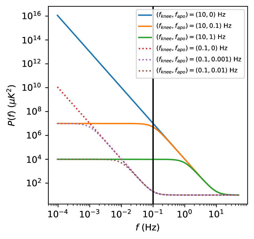
Figure 1: Noise power spectra that we use in our map-making simulations. These show a variety of low-frequency behavior, parameterized by Eq. 9, with white noise at high frequency and a low-frequency power-law slope $\alpha=3$. Here we show two knee frequencies, $f_{\text{knee}}=10$ Hz (solid lines) and $f_{\text{knee}}=0.1$ Hz (dashed lines). For each knee frequency, we have shown an unflattened spectrum ($f_{\text{apo}}=0$ Hz), and two flattened ones ($f_{\text{apo}}=0.1f_{\text{knee}}$ and $0.01f_{\text{knee}}$). The vertical line shows our scanning frequency.

To compare these algorithms, we need to do some simple simulations of scanning processes, and generate the time ordered data from a random sky signal. Our sky is a small rectangular area, with two orthogonal directions $x$ and $y$, both with range from $-1\degree$ to $+1\degree$. The signal has Stokes parameters $(I,Q,U)$ for intensity and linear polarization.

For the scanning process, our mock telescope contains nine detectors, each with different sensitivity to polarization $Q$ and $U$. It scans the sky with a raster scanning pattern. Its scanning frequency is $f_{\text{scan}}=0.1$ Hz and sampling frequency is $f_{\text{sample}}=100$ Hz. The telescope scans the sky horizontally then vertically. This gives the noiseless signal $\mathbf{s}$. The sky signal in the timestream has a root-mean-square (RMS) of $56$ $\mu$K. The signal is continuous, so that it has structure on sub-pixel scales, but we find that our main conclusions remain the same when the input signal is pixelized. In map-making, we digitize the position $(x,y)$ into $512\times 512$ pixels.

We model the noise power spectrum with

$$P(f)=\sigma^{2}\quantity(1+\frac{f_{\text{knee}}^{\alpha}+f_{\text{apo}}^{\alpha}}{f^{\alpha}+f_{\text{apo}}^{\alpha}})$$ (9)

which is white at high frequencies, a power law below the knee frequency, and gives us the option to flatten the low-frequency noise below an apodization frequency (like in Papež et al., 2018). Note that as $f_{\text{apo}}\rightarrow 0$, $P(f)\rightarrow\sigma^{2}\quantity(1+(f/f_{\text{knee}})^{-\alpha})$, and it becomes a $1/f$-type noise model.

Dünner et al. (2013) measured the slopes of the atmospheric noise in the Atacama under different water vapor conditions, finding $\alpha=2.7$ to $2.9$. Here we use $\sigma^{2}=10$ $\mu$K², $\alpha=3$, and compare the performance under different noise models. In our calculations, we choose different combinations of $f_{\text{knee}}$ and $f_{\text{apo}}$ as in Figure 1. The noise spectra with the most low frequency noise have high $f_{\text{knee}}$ or low cut-off $f_{\text{apo}}$.

The noise covariance matrix

$$N_{ff^{\prime}}=P(f)\frac{\delta_{ff^{\prime}}}{\Delta_{f}}$$ (10)

is a diagonal matrix in frequency space, where $\Delta_{f}$ is equal to the reciprocal of total scanning time $T\approx 1.05\times 10^{4}$ seconds.

Finally, we get the simulated time ordered data $\mathbf{d}=\mathbf{s}+\mathbf{n}$ by adding up the signal and noise.

3 Results

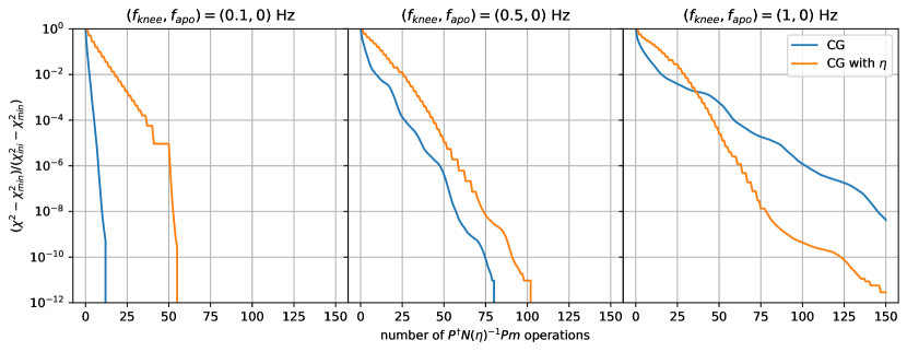
Figure 2: Convergence properties depend on the amount of low-frequency noise, which increases from the left panel to the right panel with increasing knee frequency. The map-making equation 2 minimize the $\chi^{2}(\mathbf{m})$, so the curve which falls fastest versus the number of operations is the preferred method. We compare the traditional conjugate gradient method (“CG,” blue line) with the parameterized conjugate gradient method (“CG with $\eta$,” orange line) under different $1/f$ noise models (fixed $f_{\text{apo}}=0$ Hz but different $f_{\text{knee}}$ in Eq. 9). When $f_{\text{knee}}\gtrsim 10\,f_{\text{scan}}=1$ Hz, the significant amount of low-frequency noise causes the parameterized conjugate gradient method to start showing its advantage. The vertical axis is rescaled such that all curves start from 1.

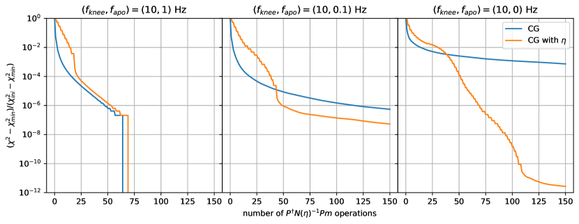
Figure 3: Like Figure 2, low-frequency noise increases from left to right, but by flattening the low-frequency noise at an apodization frequency. Low-frequency noise increases with decreasing apodization frequency (compare Figure 1). We again compare the traditional conjugate gradient method (“CG,” blue line) with the parameterized conjugate gradient method (“CG with $\eta$,” orange line). When $f_{\text{apo}}$ is much smaller than $f_{\text{knee}}$, there is a lot of low-frequency noise and the parameterized conjugate gradient method is better (ultimately falls faster) than the traditional one.

We compare the standard conjugate gradient method versus the conjugate gradient with our perturbed linear system. Both methods use the simple preconditioner $P^{\dagger}P$. Figure 2 shows the $\chi^{2}$ results for $1/f$ noise models ($f_{\text{apo}}=0$) with different knee frequencies. Note that the $\chi^{2}$ values in all figures are calculated based on the standard $\chi^{2}(\mathbf{m})$ in Eq. 3, not the $\eta$-dependent $\chi^{2}(\mathbf{m},\eta)$ of the modified system (Eq. A1). The minimum $\chi^{2}_{\text{min}}$ that we use for comparison is calculated from a deliberately slowed and well-converged parameterized conjugate gradient method: one with 100 $\eta$ values and that halts when the final norm of the residual $\norm{\mathbf{r}(\mathbf{m},1)}$ is smaller than $10^{-5}\times\norm{P^{\dagger}N^{-1}\mathbf{d}}$, or 100 iterations after $\eta=1$. From Figure 2, we can see for the $1/f$ noise model, when $f_{\text{knee}}\gtrsim 10f_{\text{scan}}$ the parameterized method starts showing an advantage over the vanilla conjugate gradient method.

In Figure 3, we fixed $f_{\text{knee}}=10$ Hz, and change $f_{\text{apo}}$. As we decrease $f_{\text{apo}}$ relative to $f_{\text{knee}}$, increasing the amount of low-frequency noise, the parameterized conjugate gradient method performs better.

Looking at the power spectrum in Figure 1, when $f_{\text{knee}}$ is small, or $f_{\text{apo}}$ is large, there is not much low-frequency noise. These situations corrrespond to the left-side plots in Figure 2 and Figure 3. The right-side graphs have significant amount of low frequency noise. We conclude that the introduction of the slowly-varying $\eta$ parameter improves performance most when there are large low-frequency noise contributions.

We also tried different $1/f$ noise slopes $\alpha$. For $\alpha=2$, the conclusion is the same as $\alpha=3$. When $\alpha=1$, the low-frequency noise is reduced compared to the cases with steeper slopes, and the vanilla conjugate gradient method is preferred, except some cases with very large knee frequency like $f_{\text{knee}}=100$ Hz and $f_{\text{apo}}=0$ which favors the parameterized method. In Papež et al. (2018), the slope $\alpha=1$ and the noise power spectrum is flattened at $f_{\text{apo}}\approx 0.1f_{\text{knee}}$. Their knee frequency is the same as their scanning frequency, so is most like our case when $f_{\text{knee}}=f_{\text{scan}}=0.1$ Hz. Their case had little low-frequency noise, and we confirm their specific result that the standard conjugate gradient method converges faster in that case. In general, however, we find cases with significantly more low-frequency noise benefit from the cooling/parameterized approach.

4 Conclusions

We analyzed the parameterized conjugate gradient map-making method that is inspired by the messenger-field idea of separating the white noise out of the noise covariance matrix. Then we gave an analytical expression for the series of $\eta$ parameters that govern how quickly the modified covariance adjusts to the correct covariance, and showed that this method adds only the extra computational cost of re-initializing the conjugate gradient process based on a new $\eta$ parameter.

We tested this method for different noise power spectra, both flattened and non-flattened at low frequency. The results showed that the parameterized method is faster than the traditional conjugate gradient method when there is a significant amount of low-frequency noise. It could be further improved if we could get a more accurate estimation for the change in $\chi^{2}$ as a function of the $\eta$ parameter, either before iteration or without using time ordered data during iteration.

Also note that we fixed the preconditioner as $M=P^{\dagger}P$ during our calculation, this parameterizing process could be applied to any preconditioner and possibly improve performance when there is significant amount of low-frequency noise.

This type of analysis for the cooling parameter may also be apply to other areas, like the Wiener filter. Papež et al. (2018) showed that the messenger field method of Elsner & Wandelt (2013) for solving Wiener filter problem could also be written as a parameterized conjugate gradient algorithm. It stands to reason that such a system may also benefit from splitting and parameterizing its noise covariance, depending on the noise properties. (In the Wiener filter, Kodi Ramanah et al. (2017) additionally suggests the splitting the signal covariance and combining the uniform parts of the signal and noise.)

The benefits to map-making from a cooled messenger method seem to come from the cooling and not actually from the messenger field that inspired it. However, the messenger field approach may still have a role in the production and analysis of CMB maps. In particular, the close connection between the messenger method and Gibbs sampling may allow us to cheaply generate noise realizations of a converged map by generating samples from the map posterior distribution, something that we will continue to explore in future work.

Appendix A The derivation of $\eta$ parameter series

We know that the initial degree of heteroscedasticity $\eta_{0}=0$, which means the system is homoscedastic (uniform noise) to start. What would be a good value for the next parameter $\eta_{1}$? To simplify notation, we use $N_{\eta}$ to denote the parameterized covariance matrix $N(\eta)=\tau I+\eta\bar{N}$. For some specific $\eta$ value, the estimated map $\mathbf{\hat{m}}(\eta)=\quantity(P^{\dagger}N_{\eta}^{-1}P)^{-1}P^{\dagger}N_{\eta}^{-1}\mathbf{d}$ minimizes

$$\begin{aligned} \chi^{2}(\mathbf{m},\eta)&=\quantity\big(\mathbf{d}-P\mathbf{m})^{\dagger}N_{\eta}^{-1}\quantity\big(\mathbf{d}-P\mathbf{m}).\end{aligned}$$ (A1)

with $\eta$ being fixed. We restrict to the case that the noise covariance matrix $N$ is diagonal in the frequency domain, and represent the frequency-domain eigenvalues as $N_{f}$.

The perturbative scheme works like this. We start with $\chi^{2}(\mathbf{\hat{m}}(\eta_{0}),\eta_{0})$ with $\mathbf{\hat{m}}(\eta_{0})=\quantity(P^{\dagger}P)^{-1}P^{\dagger}\mathbf{d}$ which could be solved directly. Then we use conjugate gradient method to find $\mathbf{\hat{m}}(\eta_{1})$ and its corresponding $\chi^{2}(\mathbf{\hat{m}}(\eta_{1}),\eta_{1})$. So let us consider $\eta_{1}=\eta_{0}+\delta\eta=\delta\eta$ such that $\eta_{1}=\delta\eta$ is very small quantity, $\delta\eta\ll 1$. (Remember $\eta_{0}=0$.) Since $\mathbf{\hat{m}}(\eta)$ minimizes $\chi^{2}(\mathbf{m},\eta)$ with $\eta$ being fixed, we have $\partialderivative{\mathbf{\hat{m}}}\chi^{2}(\mathbf{\hat{m}}(\eta),\eta)=0$, and using the chain rule

$$\derivative{\eta}\chi^{2}(\mathbf{\hat{m}}(\eta),\eta)=\partialderivative{\eta}\chi^{2}(\mathbf{\hat{m}}(\eta),\eta)=-\quantity(\mathbf{d}-P\mathbf{\hat{m}}(\eta))^{\dagger}N_{\eta}^{-1}\bar{N}N_{\eta}^{-1}(\mathbf{d}-P\mathbf{\hat{m}}(\eta))$$ (A2)

Then the fractional decrease of $\chi^{2}(\mathbf{\hat{m}}(\eta_{0}),\eta_{0})$ from $\eta_{0}$ to $\eta_{1}=\delta\eta$ is

$$-\frac{\delta\chi^{2}(\mathbf{\hat{m}}(\eta_{0}),\eta_{0})}{\chi^{2}(\mathbf{\hat{m}}(\eta_{0}),\eta_{0})}=-\delta\eta\frac{\derivative{\eta}\chi^{2}(\mathbf{\hat{m}}(\eta_{0}),\eta_{0})}{\chi^{2}(\mathbf{\hat{m}}(\eta_{0}),\eta_{0})} =\delta\eta\frac{1}{\tau}\frac{\quantity(\mathbf{d}-P\mathbf{\hat{m}}(\eta_{0}))^{\dagger}\bar{N}(\mathbf{d}-P\mathbf{\hat{m}}(\eta_{0}))}{\quantity\big(\mathbf{d}-P\mathbf{\hat{m}}(\eta_{0}))^{\dagger}\quantity\big(\mathbf{d}-P\mathbf{\hat{m}}(\eta_{0}))}$$ (A3)

Here we put a minus sign in front of this expression such that it is non-negative, and use $N_{\eta=0}=\tau I$ at the second equality. We want $\quantity|\delta\chi^{2}(\mathbf{\hat{m}}(\eta_{0}),\eta_{0})|=\chi^{2}(\mathbf{\hat{m}}(\eta_{0}),\eta_{0}))-\chi^{2}(\mathbf{\hat{m}}(\eta_{1}),\eta_{1})$ to be large to encourage fast convergence. Therefore $\chi^{2}(\mathbf{\hat{m}}(\eta_{1}),\eta_{1})$ is much smaller than $\chi^{2}(\mathbf{\hat{m}}(\eta_{0}),\eta_{0})$, or $\chi^{2}(\mathbf{\hat{m}}(\eta_{1}),\eta_{1})\ll\chi^{2}(\mathbf{\hat{m}}(\eta_{0}),\eta_{0})$. Then we would expect

$$-\frac{\delta\chi^{2}(\mathbf{\hat{m}}(0),0)}{\chi^{2}(\mathbf{\hat{m}}(0),0)}=1-\frac{\chi^{2}(\mathbf{\hat{m}}(\eta_{1}),\eta_{1})}{\chi^{2}(\mathbf{\hat{m}}(0),0)}\approx 1^{-}$$ (A4)

Here we use the notation $1^{-}$ means the upper bound is close to but strictly smaller than 1. Now we could use Eq. A3 and let it equal to $1$, then $\delta\eta=-\chi^{2}(\mathbf{\hat{m}}(\eta_{0}),\eta_{0})/\derivative{\eta}\chi^{2}(\mathbf{\hat{m}}(\eta_{0}),\eta_{0})$.

Applying this same idea to $\eta_{m+1}=\eta_{m}+\delta\eta_{m}$ with $m\geq 1$, we would get

$$\delta\eta_{m}=-\chi^{2}(\mathbf{\hat{m}}(\eta_{m}),\eta_{m})/\derivative{\eta}\chi^{2}(\mathbf{\hat{m}}(\eta_{m}),\eta_{m}).$$ (A5)

As mentioned in the main text, we need to determine the entire series $\quantity{\eta_{i}}$ before conjugate gradient iterations. We do not have the $\mathbf{\hat{m}}(\eta_{m})$ with which to calculate them and need to find another approach.

Let us go back to Eq. A3. Since we cannot calculate $\mathbf{d}-P\mathbf{\hat{m}}(\eta_{m})$ before making the map, we treat it as an arbitrary vector, then the least upper bound of Eq. A3 is given by

$$-\frac{\delta\chi^{2}(\mathbf{\hat{m}}(\eta_{0}),\eta_{0})}{\chi^{2}(\mathbf{\hat{m}}(\eta_{0}),\eta_{0})}\leq\frac{\delta\eta}{\tau}\max(\bar{N}_{f})$$ (A6)

where $\max(\bar{N}_{f})$ is the maximum eigenvalue of $\bar{N}$. We want $-\frac{\delta\chi^{2}(\mathbf{\hat{m}}(\eta_{0}),\eta_{0})}{\chi^{2}(\mathbf{\hat{m}}(\eta_{0}),\eta_{0})}$ to be as large as possible, but it won’t exceed $1$. If we combine Eq. A4 and Eq. A6, and choose $\delta\eta$ such that the least upper bound is equal to 1, to make sure the process would not going too fast. Thus we have

$$\eta_{1}=\delta\eta=\frac{\tau}{\max(\bar{N}_{f})}=\frac{\min(N_{f})}{\max(N_{f})-\min(N_{f})}.$$ (A7)

Here $N_{f}$ and $\bar{N}_{f}$ are the eigenvalues of $N$ and $\bar{N}$ in the frequency domain. If the condition number of noise covariance matrix $\kappa(N)=\max(N_{f})/\min(N_{f})\gg 1$, then $\eta_{1}\approx\kappa^{-1}(N)$.

What about the other parameters $\eta_{m}$ with $m>1$? We use a similar analysis, letting $\eta_{m+1}=\eta_{m}+\delta\eta_{m}$ with a small $\delta\eta_{m}\ll 1$. First, let us find the least upper bound

$$-\frac{\delta\chi^{2}(\mathbf{\hat{m}}(\eta_{m}),\eta_{m})}{\chi^{2}(\mathbf{\hat{m}}(\eta_{m}),\eta_{m})}= \delta\eta_{m}\frac{\quantity(\mathbf{d}-P\mathbf{\hat{m}}(\eta_{m}))^{\dagger}N_{\eta_{m}}^{-1}\bar{N}N_{\eta_{m}}^{-1}(\mathbf{d}-P\mathbf{\hat{m}}(\eta_{m}))}{\quantity\big(\mathbf{d}-P\mathbf{\hat{m}}(\eta_{m}))^{\dagger}N_{\eta_{m}}^{-1}\quantity\big(\mathbf{d}-P\mathbf{\hat{m}}(\eta_{m}))}$$ (A8)

$$\leq \delta\eta_{m}\,\max\quantity(\frac{\bar{N}_{f}}{\tau+\eta_{m}\bar{N}_{f}})$$ (A9)

The upper bound in the second line is a little bit tricky. Both matrix $\bar{N}$ and $N^{-1}_{\eta_{m}}$ can be simultaneously diagonalized in frequency space. For each eigenvector $\mathbf{e}_{f}$, the corresponding eigenvalue of the matrix on the numerator $N^{-1}_{\eta_{m}}\bar{N}N^{-1}_{\eta_{m}}$ is $\lambda_{f}=\bar{N}_{f}(\tau+\eta_{m}\bar{N}_{f})^{-2}$, and the eigenvalue for the matrix in the denominator $N^{-1}_{\eta_{m}}$ is $\gamma_{f}=(\tau+\eta_{m}\bar{N}_{f})^{-1}$. Their eigenvalues are related by $\lambda_{f}=[{\bar{N}_{f}}/{(\tau+\eta_{m}\bar{N}_{f})}]\gamma_{f}$. For any vector $\mathbf{v}=\sum_{f}\alpha_{f}\mathbf{e}_{f}$, we have

$$\frac{\mathbf{v}^{\dagger}N^{-1}_{\eta_{m}}\bar{N}N^{-1}_{\eta_{m}}\mathbf{v}}{\mathbf{v}^{\dagger}N^{-1}_{\eta_{m}}\mathbf{v}}=\frac{\sum_{f}\alpha_{f}^{2}\lambda_{f}}{\sum_{f}\alpha_{f}^{2}\gamma_{f}}=\frac{\sum_{f}\alpha_{f}^{2}\gamma_{f}\bar{N}_{f}/(\tau+\eta_{m}\bar{N}_{f})}{\sum_{f}\alpha_{f}^{2}\gamma_{f}}\leq\max\quantity(\frac{\bar{N}_{f}}{\tau+\eta_{m}\bar{N}_{f}}).$$ (A10)

Again assuming $\chi^{2}(\mathbf{\hat{m}}(\eta_{m+1}),\eta_{m+1})\ll\chi^{2}(\mathbf{\hat{m}}(\eta_{m}),\eta_{m})$, which we expect it to be satisfied for $\eta_{m}\ll 1$. That is because if $\eta\lesssim 1$, $\chi^{2}(\mathbf{\hat{m}}(\eta),\eta)$ would close to the minimum $\chi^{2}$ which means $\chi^{2}(\mathbf{\hat{m}}(\eta_{m+1}),\eta_{m+1})\lesssim\chi^{2}(\mathbf{\hat{m}}(\eta_{m}),\eta_{m})$, which would violate our assumption. Luckily, the final result (Eq. A14) is a geometric series, only the last few $\eta_{m}$ values fail to satisfy this condition. Similarly, we could set the least upper bound equal to 1. Then we get

$$\delta\eta_{m}=\min\quantity(\frac{\tau+\eta_{m}\bar{N}_{f}}{\bar{N}_{f}})=\eta_{m}+\frac{\tau}{\max(\bar{N}_{f})}.$$ (A11)

Therefore

$$\eta_{m+1}=\eta_{m}+\delta\eta_{m}=2\eta_{m}+\frac{\tau}{\max(\bar{N}_{f})}$$ (A12)

If written in the form $\eta_{m+1}+{\tau}/{\max(\bar{N}_{f})}=2\quantity(\eta_{m}+{\tau}/{\max(\bar{N}_{f})})$ it’s easy to see that for $m\geq 1$, $\eta_{m}+{\tau}/{\max(\bar{N}_{f})}$ forms a geometric series

$$\eta_{m}+\frac{\tau}{\max(\bar{N}_{f})}=\quantity(\eta_{1}+\frac{\tau}{\max(\bar{N}_{f})})2^{m-1}=\frac{\tau}{\max(\bar{N}_{f})}2^{m}$$ (A13)

where we used $\eta_{1}={\tau}/{\max(\bar{N}_{f})}$. Note that $m=0$ and $\eta_{0}=0$ also satisfy this expression and we’ve got final expression for all $\eta_{m}$

$$\eta_{m}=\min\quantity\bigg{1,\;\frac{\tau}{\max(\bar{N}_{f})}\quantity(2^{m}-1)}$$ (A14)

Here we need to truncate the series when $\eta_{m}>1$.

In numerical simulations, we find that if we update the $\eta$ parameter based on the more precise Eq. A5, there is only marginally improvements over the $\eta$ series given in Eq. A14 for the $1/f$ noise model, and slight improvements when there is not much low frequency noise. If we use Eq. A5, it ends up with fewer $\eta$ parameters in the series, but the interval between $\eta_{i}$ and $\eta_{i+1}$ gets larger. In our simulation this sometimes causes one more iteration at certain $\eta$ value, so in the end there is only slight improvements. For large data set that need lots of iterations to converge from $\eta_{i}$ to $\eta_{i+1}$, where several extra iterations may not be significant, using Eq. A5 may provide a larger performance boost.

References

- Dünner et al. (2013) Dünner, R., Hasselfield, M., Marriage, T. A., et al. 2013, ApJ, 762, 10, doi: 10.1088/0004-637X/762/1/10
- Elsner & Wandelt (2013) Elsner, F., & Wandelt, B. D. 2013, A&A, 549, A111, doi: 10.1051/0004-6361/201220586
- Huffenberger & Næss (2018) Huffenberger, K. M., & Næss, S. K. 2018, The Astrophysical Journal, 852, 92, doi: 10.3847/1538-4357/aa9c7d
- Janssen & Gulkis (1992) Janssen, M. A., & Gulkis, S. 1992, in NATO Advanced Science Institutes (ASI) Series C, ed. M. Signore & C. Dupraz, Vol. 359 (Springer), 391–408
- Kodi Ramanah et al. (2017) Kodi Ramanah, D., Lavaux, G., & Wandelt, B. D. 2017, MNRAS, 468, 1782, doi: 10.1093/mnras/stx527
- Papež et al. (2018) Papež, J., Grigori, L., & Stompor, R. 2018, A&A, 620, A59, doi: 10.1051/0004-6361/201832987
- Tegmark (1997) Tegmark, M. 1997, ApJ, 480, L87, doi: 10.1086/310631