Provably Stable Flux Reconstruction High-Order Methods on Curvilinear Elements

Abstract

Provably stable flux reconstruction (FR) schemes are derived for partial differential equations cast in curvilinear coordinates. Specifically, energy stable flux reconstruction (ESFR) schemes are considered as they allow for design flexibility as well as stability proofs for the linear advection problem on affine elements. Additionally, split forms are examined as they enable the development of energy stability proofs. The first critical step proves, that in curvilinear coordinates, the discontinuous Galerkin (DG) conservative and non-conservative forms are inherently different–even under exact integration and analytically exact metric terms. This analysis demonstrates that the split form is essential to developing provably stable DG schemes on curvilinear coordinates and motivates the construction of metric dependent ESFR correction functions in each element. Furthermore, the provably stable FR schemes differ from schemes in the literature that only apply the ESFR correction functions to surface terms or on the conservative form, and instead incorporate the ESFR correction functions on the full split form of the equations. It is demonstrated that the scheme is divergent when the correction functions are only used for surface reconstruction in curvilinear coordinates. We numerically verify the stability claims for our proposed FR split forms and compare them to ESFR schemes in the literature. Lastly, the newly proposed provably stable FR schemes are shown to obtain optimal orders of convergence. The scheme loses the orders of accuracy at the equivalent correction parameter value $c$ as that of the one-dimensional ESFR scheme.

1 Introduction

The Flux Reconstruction (FR) framework, originally proposed by Huynh [1] (also referred to as lifting collocation penalty [2] or correction procedure via reconstruction [3]), has emerged as a popular FEM approach that is both simple as it can be cast in a differential collocated form and affords design flexibility, where through a choice of the correction functions, the properties of the scheme can be altered. Importantly, subsets of FR schemes have been identified as provably linearly stable (see Refs. [4, 5, 6, 7, 8]) also known as Vincent-Castonguay-Jameson-Huynh (VCJH) schemes or Energy Stable Flux Reconstruction (ESFR). Unfortunately, these proofs are limited to affine elements and hence do not apply to general curvilinear meshes.

A discretization agnostic approach for the design and analysis of arbitrarily high-order and provably stable numerical methods for linear variable coefficient problems is provided by the summation-by-parts (SBP) framework [9, 10, 11]. SBP operators are matrix difference operators that are mimetic to high-order integration by parts and when combined with appropriate interface coupling procedures, for example simultaneous approximation terms (SATs) [12, 13, 14, 15, 16, 17, 18, 19], lead to provably stable and conservative methods. FR has been cast in SBP form [20, 21, 22] as well in residual distribution schemes [23, 24, 25, 26] paving the way for a common framework to analyze high-order schemes. Moreover, discretizations having the SBP property form the foundations for nonlinearly stable schemes for nonlinear conservation laws  [27, 28, 29, 30, 18, 19, 31, 32, 33, 34, 35, 36, 37, 38].

The focus of this article is on the construction of provably stable flux reconstruction schemes in curvilinear coordinates. Since the publication by Svärd [39], the extension of stability proofs for dense-norm SBP operators, to variable coefficient problems—particularly curvilinear coordinate transformations, has received little attention in the SBP literature. Svärd [39] proved that when dense-norms, $\bm{M}$, are multiplied against a diagonal matrix containing the metric Jacobian on the mesh nodes, $\bm{J}$, the result is not a norm, i.e., $\bm{M}\bm{J}$ is not in general a norm, and therefore provable stability is lost. However, by recasting dense-norm SBP operators in staggered form and constructing metrics on the staggered grid, stability can be recovered for partial differential equations (PDE) in curvilinear coordinates discretized using dense-norm SBP operators [40]. Alternatively, Ranocha et al. [21] demonstrated in one-dimension, that for modal based operators the issue with dense-norms can be overcome by using a dense matrix, $\tilde{\bm{J}}$, such that $\bm{M}\tilde{\bm{J}}=\left(\bm{M}\tilde{\bm{J}}\right)^{\mathrm{T}}$. In a somewhat analogous way, the extension of stability proofs of ESFR schemes to curvilinear coordinates has been unclear since the ESFR norm is dense. In this paper, taking inspiration from the developments in the SBP literature and starting from the variational form, we demonstrate how to incorporate metric Jacobian dependence in dense norms, specifically those arising in ESFR schemes. In variational form, it is immediately seen that including metric Jacobian dependence does not merely correspond to right multiplying the norm matrix, but instead having the determinant of the Jacobian embedded within the integral; since the metric Jacobian is always built on the quadrature nodes and arises in the integral by transforming from the physical to the reference domain. This allows us to formulate the metric Jacobian dependent ESFR filter and the metric dependent ESFR correction functions.

The overarching objective of this paper is to develop provably stable FR discretizations on curvilinear coordinates for systems of partial differential equations. As highlighted by the SBP community [41, 42, 40], discrete integration by parts is not satisfied in the physical space for curvilinear coordinates. This is due to the physical flux never explicitly being represented by an interpolating polynomial in the physical space [43]. This distinction, to the authors’ knowledge, has not been investigated within the ESFR and DG communities [44, 45, 46, 47]. The DG strong form in reference space can be derived by either an application of integration by parts on the DG weak form in reference space or in physical space. Since the two strong DG discretizations are not equivalent [48], we present the split form in order to mimic integration by parts in the physical space. A critical result that has not been shown in the SBP literature [40, 49, 41], is that the two DG strong forms are not equivalent even under exact integration and analytically exact metric terms, making the split form essential for curvilinear high-order schemes.

In this article, we derive provably stable FR schemes on curvilinear coordinates and consider various design decisions: modal or nodal basis, uncollocated integration, different ESFR correction functions, and different volume and surface quadrature nodes. The first main insight is that the ESFR stability condition [50, 51, 5, 52] must contain metric dependence in curvilinear coordinates. Then, we demonstrate that stability cannot be achieved when the ESFR correction functions are solely used to reconstruct the flux on the surface. This issue has been presented on linear grids for Burgers’ equation by Ranocha et al. [20] and for Euler’s equations by Abe et al. [53], although neither have found a solution to satisfy stability for general ESFR in split form. In [20], the authors investigated the issue of the dense ESFR contribution to the split forms, where they proved stability only for the DG case. In [53], the authors’ numerically demonstrated stability for the “$\text{g}_{2}$ lumped-Lobatto” ESFR scheme, which is equivalent to a collocated DG scheme on Gauss-Lobatto-Legendre nodes [54] and previously shown to be stable in split form by Gassner [55]. Following the general nonlinearly stable FR framework developed in Cicchino et al. [56] for Burgers’ equation, the ESFR filter/divergence of the correction functions is incorporated on the nonlinear volume terms to ensure nonlinear stability within the broken Sobolev-norm. This differs from the literature where the ESFR correction functions were only used to reconstruct the flux on the surface [1, 2, 50, 57, 58, 3, 5, 59, 53]. In addition, the proposed scheme is in contrast from schemes where the ESFR norm was applied to the conservative discretization; either filtering the strong form surface integral [60, 47, 20, 52], or filtering the entire weak form [22]; since such stated schemes are only linearly stable.

The remainder of this article is organized as follows: In Section 2, we introduce the mathematical notations, definitions of metrics, and establish the relationships between the physical and reference spaces. In Section 3, the DG scheme is derived in both conservative and non-conservative strong forms. We subsequently prove that the two forms are inherently different under exact integration and metric terms, and introduce the DG split form. In Section 4, the classical ESFR scheme is established, and the proposed novel nonlinearly stable FR scheme is derived. In subsequent Sections 5 and 6, we provide proofs of the free-stream preservation, local and global conservation, and stability of the proposed stable FR split form. The theoretical results are numerically verified in Sec. 7, where the classical ESFR scheme in split form (ESFR filter only applied to the facet terms) diverges while, our proposed ESFR split form (ESFR filter applied to facet and volume terms) remains stable and maintains the correct orders of accuracy.

2 Math Notation and Definitions

Consider the scalar 3D conservation law,

$$\frac{\partial}{\partial t}u(\bm{x}^{c},t)+\nabla\cdot\bm{f}(u(\bm{x}^{c},t))=0,\>t\geq 0,\>\bm{x}^{c}\coloneqq[x\text{ }y\text{ }z]\in\Omega,$$

$$u(\bm{x}^{c},0)=u_{0}(\bm{x}^{c}),$$

where $\bm{f}(u(\bm{x}^{c},t))\in\mathbb{R}^{1\times d}$ stores the fluxes in each of the $d$ directions, and the superscript $c$ refers to Cartesian coordinates. In this paper row vector notation will be used. The computational domain $\bm{\Omega}^{h}$ is partitioned into $M$ non-overlapping elements, $\bm{\Omega}_{m}$, where the domain is represented by the union of the elements, i.e.

$$\bm{\Omega}\simeq\bm{\Omega}^{h}\coloneqq\bigcup_{m=1}^{M}\bm{\Omega}_{m}.$$

Each element $m$ has a surface denoted by $\bm{\Gamma}_{m}$. The global approximation, $u^{h}(\bm{x}^{c},t)$, is constructed from the direct sum of each local approximation, $u_{m}^{h}(\bm{x}^{c},t)$, i.e.

$$u(\bm{x}^{c},t)\simeq u^{h}(\bm{x}^{c},t)=\bigoplus_{m=1}^{M}u_{m}^{h}(\bm{x}^{c},t).$$

Throughout this paper, all quantities with a subscript $m$ are specifically unique to the element $m$. On each element, we represent the solution with $N_{p}$ linearly independent modal or nodal basis of a maximum order of $p$; where, $N_{p}\coloneqq(p+1)^{d}$. The solution representation is, $u_{m}^{h}(\bm{x}^{c},t)\coloneqq\sum_{i=1}^{N_{p}}{\chi}_{m,i}(\bm{x}^{c})\hat{u}_{m,i}(t).$ The elementwise residual is,

$$R_{m}^{h}(\bm{x}^{c},t)=\frac{\partial}{\partial t}u_{m}^{h}(\bm{x}^{c},t)+\nabla\cdot\bm{f}(u_{m}^{h}(\bm{x}^{c},t)).$$ (1)

The basis functions in each element are defined as,

$$\bm{\chi}(\bm{x}^{c})\coloneqq[\chi_{1}(\bm{x}^{c})\text{, }\chi_{2}(\bm{x}^{c})\text{, }\dots\text{, }\chi_{N_{p}}(\bm{x}^{c})]=\bm{\chi}({x})\otimes\bm{\chi}({y})\otimes\bm{\chi}({z})\in\mathbb{R}^{1\times N_{p}},$$ (2)

where $\otimes$ is the tensor product.

The physical coordinates are mapped to the reference element $\bm{\xi}^{r}\coloneqq\{[\xi\text{, }\eta\text{, }\zeta]:-1\leq\xi,\eta,\zeta\leq 1\}$ by

$$\bm{x}_{m}^{c}(\bm{\xi}^{r})\coloneqq\bm{\Theta}_{m}(\bm{\xi}^{r})=\sum_{i=1}^{N_{t,m}}{\Theta}_{m,i}(\bm{\xi}^{r})\hat{\bm{x}}_{m,i}^{c},$$ (3)

where ${\Theta}_{m,i}$ are the mapping shape functions of the $N_{t,m}$ physical mapping control points $\hat{\bm{x}}_{m,i}^{c}$.

To transform Eq. (1) to the reference basis, as in refs [61, 62, 63, 64, 65], we introduce the physical

$$\bm{a}_{j}\coloneqq\frac{\partial\bm{x}^{c}}{\partial\xi^{j}},\text{ }j=1,2,3$$

and reference

$$\bm{a}^{j}\coloneqq\nabla\xi^{j},\text{ }j=1,2,3$$

vector bases. We then introduce the determinant of the metric Jacobian as

$$J^{\Omega}\coloneqq|\bm{J}^{\Omega}|=\bm{a}_{1}\cdot(\bm{a}_{2}\times\bm{a}_{3}),$$ (4)

and the metric Jacobian cofactor matrix as  [61, 47, 62, 66],

$$\bm{C}^{T}\coloneqq J^{\Omega}(\bm{J}^{\Omega})^{-1}=\begin{bmatrix}J^{\Omega}\bm{a}^{1}\\ J^{\Omega}\bm{a}^{2}\\ J^{\Omega}\bm{a}^{3}\end{bmatrix}=\begin{bmatrix}J^{\Omega}\bm{a}^{\xi}\\ J^{\Omega}\bm{a}^{\eta}\\ J^{\Omega}\bm{a}^{\zeta}\end{bmatrix}.$$ (5)

The metric cofactor matrix is formulated by the “conservative curl” form from [63, Eq. 36] so as to discretely satisfy the Geometric Conservation Law (GCL)

$$\sum_{i=1}^{3}\frac{\partial(J^{\Omega}(\bm{a}^{i})_{n})}{\partial\xi^{i}}=0\text{, }n=1,2,3\Leftrightarrow\sum_{i=1}^{3}\frac{\partial}{\partial\xi^{i}}(\bm{C})_{ni}=0\text{, }n=1,2,3\Leftrightarrow\nabla^{r}\cdot(\bm{C})=\bm{0},$$ (6)

which is detailed in Sec. 5 for a fixed mesh, where $(\;)_{ni}$ represents the $n^{\text{th}}$ row, $i^{\text{th}}$ column component of a matrix.

Having established the transformations mapping the physical to the reference coordinates on each element, the differential volume and surface elements can be defined as,

$$d\bm{\Omega}_{m}=J_{m}^{\Omega}d\bm{\Omega}_{r}\text{, similarly }d\bm{\Gamma}_{m}=J_{m}^{\Gamma}d\bm{\Gamma}_{r}.$$ (7)

The reference flux for each element $m$ is defined as

$$\bm{f}_{m}^{r}=\bm{C}_{m}^{T}\cdot\bm{f}_{m}\Leftrightarrow\bm{f}_{m,j}^{r}=\sum_{i=1}^{d}(\bm{C}_{m}^{T})_{ji}\bm{f}_{m,i}\Leftrightarrow\bm{f}_{m}^{r}=\bm{f}_{m}\bm{C}_{m},$$ (8)

where the dot product notation for tensor-vector operations is introduced. The relationship between the physical and reference unit normals is given as [47, Appendix B.2],

$$\hat{\bm{n}}_{m}=\frac{1}{J_{m}^{\Gamma}}\bm{C}_{m}\cdot\hat{\bm{n}}^{r}=\frac{1}{J_{m}^{\Gamma}}\hat{\bm{n}}^{r}\bm{C}_{m}^{T},$$ (9)

for a water-tight mesh. Additionally, the definition of the divergence operator derived from divergence theorem in curvilinear coordinates can be expressed as [61, Eq. (2.22) and (2.26)],

$$\nabla\cdot\bm{f}_{m}=\frac{1}{J_{m}^{\Omega}}\nabla^{r}\cdot\Big{(}\bm{f}_{m}\bm{C}_{m}\Big{)}=\frac{1}{J_{m}^{\Omega}}\nabla^{r}\cdot\bm{f}_{m}^{r},$$ (10)

and the gradient of a scalar as [61, Eq. (2.21)],

$$\nabla{\chi}=\frac{1}{J_{m}^{\Omega}}\bm{C}_{m}\cdot\nabla^{r}\chi=\frac{1}{J_{m}^{\Omega}}\Big{(}\nabla^{r}\chi\Big{)}\bm{C}_{m}^{T}.$$ (11)

Thus, substituting Eq. (10) into Eq. (1), the reference elementwise residual is,

$$R_{m}^{h,r}(\bm{\xi}^{r},t)\coloneqq R_{m}^{h}(\bm{\Theta}_{m}(\bm{\xi}^{r}),t)=\frac{\partial}{\partial t}u_{m}^{h}(\bm{\Theta}_{m}(\bm{\xi}^{r}),t)+\frac{1}{J_{m}^{\Omega}}\nabla^{r}\cdot\bm{f}^{r}(u_{m}^{h}(\bm{\Theta}_{m}(\bm{\xi}^{r}),t)).$$ (12)

3 Discontinuous Galerkin

In this section we present a provably stable DG discretization for curvilinear coordinates [40, 49, 41] to act as the cornerstone for our provably stable FR schemes. We derive the DG strong form for both “conservative” and “non-conservative” formulations, and prove that they are inherently different for curvilinear coordinates; even with analytically exact metric terms and exact integration. This difference necessitates a split form to ensure nonlinear stability on curvilinear coordinates. Specifically we cover:

1. Deriving the conservative DG strong form by transforming the physical DG weak form to reference space. Then, projecting the reference flux onto the reference polynomial basis, and finally, integrating the volume terms by parts in the reference space.

2. Deriving the non-conservative DG strong form by projecting the physical flux onto a physical basis in the physical DG weak form. Then integrating the volume terms by parts in the physical space, and finally, transforming the physical DG non-conservative strong form to the reference space.

3. Comparing the two forms, prove that they are inherently different, even under exact integration with analytically exact metric terms, and that discrete integration by parts in the physical space is not satisfied for either form. Then, combining the two forms to discretely “mimic” integration by parts in the physical space.

3.1 DG - Conservative Strong Form

In a Galerkin framework, we left multiply the physical residual Eq. (1) by an orthogonal test function. Choosing the test function to be the same as the basis function, integrating in physical space, and applying integration by parts in physical space, we arrive at the weak form,

$$\begin{split}\int_{\bm{\Omega}_{m}}{\chi}_{m,i}(\bm{x}^{c})\frac{\partial}{\partial t}u_{m}^{h}(\bm{x}^{c},t)d\bm{\Omega}_{m}-\int_{\bm{\Omega}_{m}}\nabla{\chi}_{m,i}(\bm{x}^{c})\cdot\bm{f}(u_{m}^{h}(\bm{x}^{c},t))d\bm{\Omega}_{m}+\int_{\bm{\Gamma}_{m}}{\chi}_{m,i}(\bm{x}^{c})\hat{\bm{n}}_{m}\cdot\bm{f}^{*}(u_{m}^{h}(\bm{x}^{c},t))d\bm{\Gamma}_{m}={0},\\ \forall i=1,\dots,N_{p}\end{split}$$ (13)

where $\bm{f}^{*}(u_{m}^{h}(\bm{x}^{c},t))$ represents the physical numerical flux.

Now, we transform the physical DG weak form, Eq. (13), to the reference space, by using the definitions of the differential volume and surface elements, physical gradient operator and physical unit normals (Equations (7), (9), (11)),

$$\begin{split}\int_{\bm{\Omega}_{r}}{\chi}_{i}(\bm{\xi}^{r})J_{m}^{\Omega}\frac{\partial}{\partial t}u_{m}^{h}(\bm{\Theta}_{m}(\bm{\xi}^{r}),t)d\bm{\Omega}_{r}-\int_{\bm{\Omega}_{r}}\Big{(}\frac{1}{J_{m}^{\Omega}}\nabla^{r}{\chi}_{i}(\bm{\xi}^{r})\bm{C}_{m}^{T}\Big{)}J_{m}^{\Omega}\cdot\bm{f}(u_{m}^{h}(\bm{\Theta}_{m}(\bm{\xi}^{r}),t))d\bm{\Omega}_{r}\\ +\int_{\bm{\Gamma}_{r}}{\chi}_{i}(\bm{\xi}^{r})J_{m}^{\Gamma}\frac{1}{J_{m}^{\Gamma}}\hat{\bm{n}}^{r}\bm{C}_{m}^{T}\cdot\bm{f}^{*}(u_{m}^{h}(\bm{\Theta}_{m}(\bm{\xi}^{r}),t))d\bm{\Gamma}_{r}={0},\>\forall i=1,\dots,N_{p}.\end{split}$$ (14)

Notice the change of variables since $\bm{\chi}_{m}(\bm{x}^{c})\coloneqq\bm{\chi}(\bm{\Theta}_{m}^{-1}(\bm{x}^{c}))$ are implicitly defined through polynomial basis functions in the reference space. From the definition Eq. (8), the reference flux is substituted for $\bm{C}_{m}^{T}\cdot\bm{f}(u_{m}^{h}(\bm{\Theta}_{m}(\bm{\xi}^{r}),t))$ in the volume integral. We then project the reference flux in Eq. (14) onto the reference polynomial basis functions, and substitute the basis expansion for the solution. The variational DG weak form in reference space is thus,

$$\begin{split}\int_{\bm{\Omega}_{r}}{\chi}_{i}(\bm{\xi}^{r})J_{m}^{\Omega}\bm{\chi}(\bm{\xi}^{r})\frac{d}{dt}\hat{\bm{u}}_{m}(t)^{T}d\bm{\Omega}_{r}-\int_{\bm{\Omega}_{r}}\nabla^{r}{\chi}_{i}(\bm{\xi}^{r})\cdot\bm{\chi}(\bm{\xi}^{r})\hat{\bm{f}}_{m}^{r}(t)^{T}d\bm{\Omega}_{r}+\int_{\bm{\Gamma}_{r}}{\chi}_{i}(\bm{\xi}^{r})\hat{\bm{n}}^{r}\bm{C}_{m}^{T}\cdot\bm{f}_{m}^{*}(u_{m}^{h}(\bm{\Theta}_{m}(\bm{\xi}^{r}),t))d\bm{\Gamma}_{r}={0},\\ \>\forall i=1,\dots,N_{p}.\end{split}$$ (15)

Next Eq. (15), the reference DG weak form, is integrated by parts in the reference space resulting in,

$$\begin{split}\int_{\bm{\Omega}_{r}}{\chi}_{i}(\bm{\xi}^{r})J_{m}^{\Omega}\bm{\chi}(\bm{\xi}^{r})\frac{d}{dt}\hat{\bm{u}}_{m}(t)^{T}d\bm{\Omega}_{r}+\int_{\bm{\Omega}_{r}}{\chi}_{i}(\bm{\xi}^{r})\Bigg{(}\sum_{j=1}^{N_{p}}\nabla^{r}{\chi}_{j}(\bm{\xi}^{r})\cdot\hat{\bm{f}}_{m,j}^{r}(t)\Bigg{)}d\bm{\Omega}_{r}+\int_{\bm{\Gamma}_{r}}{\chi}_{i}(\bm{\xi}^{r})\Big{[}\hat{\bm{n}}^{r}\bm{C}_{m}^{T}\cdot\bm{f}^{*}_{m}-\hat{\bm{n}}^{r}\cdot\bm{\chi}(\bm{\xi}^{r})\bm{\hat{f}}^{r}_{m}(t)^{T}\Big{]}d\bm{\Gamma}_{r}={0},\\ \forall i=1,\dots,N_{p}.\end{split}$$ (16)

In the general case, the interpolation of the nonlinear reference flux to the face does not equal the metric terms evaluated at the face multiplied with the flux on the face.

Next, we introduce $N_{vp}$ volume and $N_{fp}$ facet cubature nodes, $\bm{\xi}_{v}^{r}$ and $\bm{\xi}_{f,k}^{r}$ respectively. We also introduce $\bm{W}$ and $\bm{J}_{m}$ as diagonal operators storing the quadrature weights and the determinant of the metric Jacobian at the volume cubature nodes. We present the discretization of Eq. (16), the discrete conservative DG strong form, as

$$\bm{M}_{m}\frac{d}{dt}\hat{\bm{u}}_{m}(t)^{T}+\bm{S}_{\xi}\hat{\bm{f}}_{1m}^{r}(t)^{T}+\bm{S}_{\eta}\hat{\bm{f}}_{2m}^{r}(t)^{T}+\bm{S}_{\zeta}\hat{\bm{f}}_{3m}^{r}(t)^{T}+\sum_{f=1}^{N_{f}}\sum_{k=1}^{N_{fp}}\bm{\chi}(\bm{\xi}_{f,k}^{r})^{T}{W}_{f,k}[\hat{\bm{n}}^{r}\bm{C}_{m}(\bm{\xi}_{f,k}^{r})^{T}\cdot\bm{f}^{*}_{m}-\hat{\bm{n}}^{r}\cdot\bm{\chi}(\bm{\xi}_{f,k}^{r})\hat{\bm{f}}^{r}_{m}(t)^{T}]=\bm{0}^{T},$$ (17)

where $N_{f}$ represents the number of faces on the element. The discrete mass and stiffness matrices are defined as,

$$(\bm{M}_{m})_{ij}\approx\int_{\Omega_{r}}J_{m}^{\Omega}{\chi}_{i}(\bm{\xi}^{r}){\chi}_{j}(\bm{\xi}^{r})d\Omega_{r}\to\bm{M}_{m}=\bm{\chi}(\bm{\xi}_{v}^{r})^{T}\bm{W}\bm{J}_{m}\bm{\chi}(\bm{\xi}_{v}^{r}),$$

$$(\bm{S}_{\xi})_{ij}=\int_{\Omega_{r}}{\chi}_{i}(\bm{\xi}^{r})\frac{\partial}{\partial\xi}{\chi}_{j}(\bm{\xi}^{r})d\Omega_{r}\rightarrow\bm{S}_{\xi}=\bm{\chi}(\bm{\xi}_{v}^{r})^{T}\bm{W}\bm{\chi}_{\xi}(\bm{\xi}_{v}^{r}),$$

and similarly for the other reference directions. The equality for the stiffness matrices holds for quadrature rules of at least $2p-1$ in strength. Furthermore, we introduce the $\text{L}_{2}$ projection operator as $\bm{\Pi}\coloneqq\bm{M}^{-1}\bm{\chi}(\bm{\xi}_{v}^{r})^{T}\bm{W}$, where the metric independent mass matrix is $\bm{M}=\bm{\chi}(\bm{\xi}_{v}^{r})^{T}\bm{W}\bm{\chi}(\bm{\xi}_{v}^{r})$. Thus, the modal coefficients of the reference flux are the $\text{L}_{2}$ projection of the reference flux, $\hat{\bm{f}}_{m}^{r}(t)^{T}=\bm{\Pi}(\bm{f}_{m}^{r^{T}})$.

3.2 DG - Non-Conservative Strong Form

Returning to the physical DG weak form, Eq. (13), as discussed in [43, 67], there is no claim that the physical flux has a polynomial basis function expansion for curvilinear elements. We term the scheme “non-conservative” because it does not recover the definition of the reference divergence operator in Eq. (10) [40, 49]. Following the approach in [45, 46], we substitute the solution expansion and project the physical flux onto the basis functions. Eq. (13) is integrated by parts in physical space and yields the “non-conservative” DG strong form in physical space,

$$\begin{split}\int_{\bm{\Omega}_{m}}{\chi}_{m,i}(\bm{x}^{c})\bm{\chi}_{m}(\bm{x}^{c})\frac{d}{dt}\hat{\bm{u}}_{m}(t)^{T}d\bm{\Omega}_{m}+\int_{\bm{\Omega}_{m}}{\chi}_{m,i}(\bm{x}^{c})\Big{(}\sum_{j=1}^{N_{p}}\nabla{\chi}_{m,j}(\bm{x}^{c})\cdot\hat{\bm{f}}_{m,j}(t)\Big{)}d\bm{\Omega}_{m}+\int_{\bm{\Gamma}_{m}}{\chi}_{m,i}(\bm{x}^{c})\hat{\bm{n}}_{m}\cdot(\bm{f}^{*}_{m}-\bm{f}_{m})d\bm{\Gamma}_{m}={0},\\ \>\forall i=1,\dots,N_{p}.\end{split}$$ (18)

To discretely represent the derivative of the physical flux in the physical space, it must be represented by the derivative of a basis expansion in the physical space multiplied by its modal coefficients. Although in the continuous sense the physical divergence operator could be recovered by commuting the basis functions across the dot product in Eq. (18); doing so would remove the claim that the physical flux has a basis function expansion. Only in the reference space can the basis function be brought across the dot product since the derivative of a polynomial basis function on the reference element exist. Thus, discretely applying integration by parts in the physical space to arrive at Eq. (18) would necessitate that $\bm{\chi}_{m}(\bm{x}^{c})=\bm{\chi}(\bm{\Theta}_{m}^{-1}(\bm{x}^{c}))$ is a polynomial basis. It is clear when transforming Eq. (18) to the reference space, and substituting the definition of the gradient for curvilinear elements, Eq. (11), that it is inconsistent with the previous formulation in Eq. (16),

$$\begin{split}\int_{\bm{\Omega}_{r}}{\chi}_{i}(\bm{\xi}^{r})J_{m}^{\Omega}\bm{\chi}(\bm{\xi}^{r})\frac{d}{dt}\hat{\bm{u}}_{m}(t)^{T}d\bm{\Omega}_{r}+\int_{\bm{\Omega}_{r}}{\chi}_{i}(\bm{\xi}^{r})\Bigg{(}\sum_{j=1}^{N_{p}}\Big{(}\nabla^{r}{\chi}_{j}(\bm{\xi}^{r})\bm{C}_{m}^{T}\Big{)}\cdot\hat{\bm{f}}_{m,j}(t)\Bigg{)}d\bm{\Omega}_{r}+\int_{\bm{\Gamma}_{r}}{\chi}_{i}(\bm{\xi}^{r})\hat{\bm{n}}^{r}\bm{C}_{m}^{T}\cdot(\bm{f}^{*}_{m}-\bm{f}_{m})d\bm{\Gamma}_{r}={0},\\ \>\forall i=1,\dots,N_{p}.\end{split}$$ (19)

Explicitly, the metric cofactor matrix appears on the outside of the reference divergence/gradient operator. Only if the mesh is linear, skew-symmetric, or symmetric with uniform constant wave speeds for linear advection, will the volume integrals in Equations (16) and (19) be equivalent in discrete form.

Theorem 1.

The volume terms in Eq. (16) and Eq. (19) are inherently different for a curvilinear mesh; even with exact integration and exact metric terms.

Proof.

Consider just one of the divergence terms in the volume integral,

$$\begin{split}\text{Conservative DG: }\sum_{k=1}^{d}\int_{\bm{\Omega}_{r}}\chi_{i}(\bm{\xi}^{r})\sum_{j=1}^{N_{p}}\frac{\partial\chi_{j}(\bm{\xi}^{r})}{\partial\xi_{k}}\Bigg{[}\bm{\Pi}\Big{(}{J}_{m}^{\Omega}\frac{\partial\xi_{k}}{\partial x}\bm{f}_{x}(u_{m}^{h})\Big{)}\Bigg{]}_{j}d\bm{\Omega}_{r},\\ \text{Non-Conservative DG: }\sum_{k=1}^{d}\int_{\bm{\Omega}_{r}}\chi_{i}(\bm{\xi}^{r})J_{m}^{\Omega}\frac{\partial\xi_{k}}{\partial x}\sum_{j=1}^{N_{p}}\frac{\partial\chi_{j}(\bm{\xi}^{r})}{\partial\xi_{k}}\Bigg{[}\bm{\Pi}\Big{(}\bm{f}_{x}(u_{m}^{h})\Big{)}\Bigg{]}_{j}d\bm{\Omega}_{r}.\end{split}$$ (20)

If we are to consider both exact integration and exact metric terms ($J_{m}^{\Omega}\frac{\partial\xi_{k}}{\partial x}$), then the two forms cannot be equivalent for a general $f_{x}(u_{m}^{h})$.

∎

Remark 1.

Only for the specific case of linear advection with a polynomial representation of the mesh can the two forms be equivalent through polynomial exactness; provided they are both exactly integrated and the nonlinear term in the conservative form is projected onto a sufficiently high polynomial space.

3.3 DG - Split Form

For the objective of developing provably stable schemes, alike  [41, 68, 49], we introduce the split form by adding a half of the conservative DG Strong form Eq. (16) with the non-conservative DG Strong form Eq. (19) to discretely satisfy integration by parts,

$$\begin{split}\int_{\bm{\Omega}_{r}}{\chi}_{i}(\bm{\xi}^{r})J_{m}^{\Omega}\bm{\chi}(\bm{\xi}^{r})\frac{d}{dt}\hat{\bm{u}}_{m}(t)^{T}d\bm{\Omega}_{r}+\frac{1}{2}\int_{\bm{\Omega}_{r}}{\chi}_{i}(\bm{\xi}^{r})\Bigg{(}\sum_{j=1}^{N_{p}}\nabla^{r}{\chi}_{j}(\bm{\xi}^{r})\cdot\hat{\bm{f}}_{m,j}^{r}(t)\Bigg{)}d\bm{\Omega}_{r}+\frac{1}{2}\int_{\bm{\Omega}_{r}}{\chi}_{i}(\bm{\xi}^{r})\Bigg{(}\sum_{j=1}^{N_{p}}\Big{(}\nabla^{r}{\chi}_{j}(\bm{\xi}^{r})\bm{C}_{m}^{T}\Big{)}\cdot\hat{\bm{f}}_{m,j}(t)\Bigg{)}d\bm{\Omega}_{r}\\ +\int_{\bm{\Gamma}_{r}}{\chi}_{i}(\bm{\xi}^{r})^{T}\Big{[}\hat{\bm{n}}^{r}\bm{C}_{m}^{T}\cdot(\bm{f}^{*}_{m}-\frac{1}{2}\bm{f}_{m})-\hat{\bm{n}}^{r}\cdot\frac{1}{2}\bm{\chi}(\bm{\xi}^{r})\hat{\bm{f}}^{r}_{m}(t)^{T}\Big{]}d\bm{\Gamma}_{r}={0},\>\forall i=1,\dots,N_{p}.\end{split}$$ (21)

Note that the surface splitting naturally accommodates arbitrary sets of volume and facet cubature nodes. Recasting Eq. (21) into discrete form by evaluating at volume and facet cubature nodes, we have the DG split form,

$$\begin{split}\bm{M}_{m}\frac{d}{dt}\hat{\bm{u}}_{m}(t)^{T}+\frac{1}{2}\bm{\chi}(\bm{\xi}_{v}^{r})^{T}\bm{W}\nabla^{r}\bm{\chi}(\bm{\xi}_{v}^{r})\cdot\hat{\bm{f}}_{m}^{r}(t)^{T}+\frac{1}{2}\bm{\chi}(\bm{\xi}_{v}^{r})^{T}\bm{W}\tilde{\nabla}^{r}\bm{\chi}(\bm{\xi}_{v}^{r})\cdot\hat{\bm{f}}_{m}(t)^{T}+\sum_{f=1}^{N_{f}}\sum_{k=1}^{N_{fp}}\bm{\chi}(\bm{\xi}_{f,k}^{r})^{T}W_{f,k}[\hat{\bm{n}}^{r}\cdot\bm{f}^{C,r}_{m}]=\bm{0}^{T},\end{split}$$ (22)

where we introduced $\tilde{\nabla}^{r}\bm{\chi}(\bm{\xi}_{v}^{r})=\begin{pmatrix}\nabla^{r}{\chi}_{1}(\bm{\xi}_{v,1}^{r})\bm{C}_{m}(\bm{\xi}_{v,1}^{r})^{T}&\dots&\nabla^{r}{\chi}_{N_{p}}(\bm{\xi}_{v,1}^{r})\bm{C}_{m}(\bm{\xi}_{v,1}^{r})^{T}\\ \vdots&\ddots&\vdots\\ \nabla^{r}{\chi}_{1}(\bm{\xi}_{v,N_{vp}}^{r})\bm{C}_{m}(\bm{\xi}_{v,N_{vp}}^{r})^{T}&\dots&\nabla^{r}{\chi}_{N_{p}}(\bm{\xi}_{v,N_{vp}}^{r})\bm{C}_{m}(\bm{\xi}_{v,N_{vp}}^{r})^{T}\end{pmatrix}$ to store the transformed reference gradient of the basis functions evaluated at volume cubature nodes. Also, we introduced
$\bm{f}^{C,r}_{m}=\bm{f}^{*}_{m}\bm{C}_{m}(\bm{\xi}_{f,k}^{r})-\frac{1}{2}\bm{f}_{m}\bm{C}_{m}(\bm{\xi}_{f,k}^{r})-\frac{1}{2}\bm{\chi}(\bm{\xi}_{f,k}^{r})\bm{\hat{f}}_{m}^{r}(t)^{T}$ as the difference between the reference transformation of the physical numerical flux, the physical flux and the interpolated reference flux on the face.

4 Energy Stable Flux Reconstruction

4.1 ESFR - Classical Formulation

Following an ESFR framework, the reference flux is composed of a discontinuous and a corrected component,

$$\bm{f}^{r}(u_{m}^{h}(\bm{\Theta}_{m}(\bm{\xi}^{r}),t))\coloneqq\bm{f}^{D,r}(u_{m}^{h}(\bm{\Theta}_{m}(\bm{\xi}^{r}),t))+\sum_{f=1}^{N_{f}}\sum_{k=1}^{N_{f_{p}}}\bm{g}^{f,k}(\bm{\xi}^{r})[\hat{\bm{n}}^{r}\cdot({\bm{f}}_{m}^{*,r}-{\bm{f}}_{m}^{r})].$$ (23)

The vector correction functions $\bm{g}^{f,k}(\bm{\xi}^{r})\in\mathbb{R}^{1\times d}$ associated with face $f$, facet cubature node $k$ in the reference element, are defined as the tensor product of the $p+1$ order one-dimensional correction functions ($\bm{\phi}$ stores a basis of order $p+1$), with the corresponding $p$-th order basis functions in the other reference directions.

$$\begin{split}\bm{g}^{f,k}(\bm{\xi}^{r})=[\Big{(}\bm{\phi}(\xi)\otimes\bm{\chi}({\eta})\otimes\bm{\chi}({\zeta})\Big{)}\Big{(}\hat{\bm{g}}^{f,k}_{1}\Big{)}^{T},\Big{(}\bm{\chi}({\xi})\otimes\bm{\phi}(\eta)\otimes\bm{\chi}({\zeta})\Big{)}\Big{(}\hat{\bm{g}}^{f,k}_{2}\Big{)}^{T},\Big{(}\bm{\chi}({\xi})\otimes\bm{\chi}({\eta})\otimes\bm{\phi}(\zeta)\Big{)}\Big{(}\hat{\bm{g}}^{f,k}_{3}\Big{)}^{T}]\\ =[{g}^{f,k}_{1}(\bm{\xi}^{r}),{g}^{f,k}_{2}(\bm{\xi}^{r}),{g}^{f,k}_{3}(\bm{\xi}^{r})],\end{split}$$ (24)

such that

$$\bm{g}^{f,k}(\bm{\xi}_{f_{i},k_{j}}^{r})\cdot\hat{\bm{n}}^{r}_{f_{i},k_{j}}=\begin{cases}1,\;\;\text{ if }f_{i}=f,\text{ and }k_{j}=k\\ 0,\;\;\text{ otherwise.}\end{cases}$$ (25)

Coupled with the symmetry condition $g^{L}(\xi^{r})=-g^{R}(-\xi^{r})$ to satisfy Eq. (25), the one-dimensional ESFR fundamental assumption from [50] is,

$$\int_{-1}^{1}\nabla^{r}{\chi}_{i}({\xi}^{r}){g}^{f,k}({\xi}^{r})d\xi-c\frac{\partial^{p}{\chi}_{i}({\xi}^{r})^{T}}{\partial\xi^{p}}\frac{\partial^{p+1}{g}^{f,k}({\xi}^{r})}{\partial\xi^{p+1}}={0},\>\forall i=1,\dots,N_{p},$$ (26)

and similarly for the other reference directions.

Akin to [51, 5], consider introducing the differential operator,

$$\begin{split}&\text{2D:}\indent\partial^{(s,v)}=\frac{\partial^{s+v}}{\partial\xi^{s}\partial\eta^{v}},\>\text{such that }s=\{0,p\},\>v=\{0,p\},\>s+v\geq p,\\ &\text{3D:}\indent\partial^{(s,v,w)}=\frac{\partial^{s+v+w}}{\partial\xi^{s}\partial\eta^{v}\partial\zeta^{w}},\>\text{such that }s=\{0,p\},\>v=\{0,p\},\>w=\{0,p\},\>s+v+w\geq p,\end{split}$$ (27)

with its corresponding correction parameter

$$\begin{split}&\text{2D:}\indent c_{(s,v)}=c_{1D}^{(\frac{s}{p}+\frac{v}{p})},\\ &\text{3D:}\indent c_{(s,v,w)}=c_{1D}^{(\frac{s}{p}+\frac{v}{p}+\frac{w}{p})}.\end{split}$$ (28)

Note that the total degree is $dim\times p$ for a tensor-product basis that is of order $p$ in each direction.

For example,

$$\partial^{(0,p,0)}=\frac{\partial^{p}}{\partial\eta^{p}},\>c_{(0,p,0)}=c_{1D},\>\partial^{(p,0,p)}=\frac{\partial^{2p}}{\partial\xi^{p}\partial\zeta^{p}},\>c_{(p,0,p)}=c_{1D}^{2},\>\partial^{(p,p,p)}=\frac{\partial^{3p}}{\partial\xi^{p}\partial\eta^{p}\partial\zeta^{p}},\>c_{(p,p,p)}=c_{1D}^{3}.$$

Since $\int_{\bm{\Omega}_{r}}\partial^{(s,v,w)}\bm{\chi}(\bm{\xi}^{r})^{T}\partial^{(s,v,w)}\Big{(}\nabla^{r}\bm{\chi}(\bm{\xi}^{r})\Big{)}d\bm{\Omega}_{r}$ composes of the complete broken Sobolev-norm for each $s$, $v$, $w$ [59, 52], the tensor product ESFR fundamental assumption, that recovers the VCJH schemes exactly for linear elements is defined as,

$$\int_{\bm{\Omega}_{r}}\nabla^{r}{\chi}_{i}(\bm{\xi}^{r})\cdot\bm{g}^{f,k}(\bm{\xi}^{r})d\bm{\Omega}_{r}-\sum_{s,v,w}c_{(s,v,w)}\partial^{(s,v,w)}{\chi}_{i}(\bm{\xi}^{r})\partial^{(s,v,w)}\Big{(}\nabla^{r}\cdot\bm{g}^{f,k}(\bm{\xi}^{r})\Big{)}={0},\>\forall i=1,\dots,N_{p},$$ (29)

where $\sum_{s,v,w}$ sums over all possible $s$, $v$, $w$ combinations in Eq. (27).

To discretely represent the divergence of the correction functions, we introduce the correction field
${h}^{f,k}(\bm{\xi}^{r})\in P_{3p}(\bm{\Omega}_{r})$ associated with the face $f$ cubature node $k$ as,

$${h}^{f,k}(\bm{\xi}^{r})=\bm{\chi}(\bm{\xi}^{r})\Big{(}\hat{\bm{h}}^{f,k}\Big{)}^{T}=\nabla^{r}\cdot\bm{g}^{f,k}(\bm{\xi}^{r}).$$ (30)

To arrive at the ESFR strong form, we substitute the ESFR reference flux, Eq. (23), into the elementwise reference residual, Eq. (12), project it onto the polynomial basis, and evaluate at cubature nodes,

$$\bm{\chi}(\bm{\xi}_{v}^{r})\frac{d}{dt}\hat{\bm{u}}_{m}(t)^{T}+\bm{J}_{m}^{-1}\nabla^{r}\bm{\chi}(\bm{\xi}_{v}^{r})\cdot\hat{\bm{f}}_{m}^{D,r}(t)^{T}+\bm{J}_{m}^{-1}\sum_{f=1}^{N_{f}}\sum_{k=1}^{N_{fp}}\bm{\chi}(\bm{\xi}_{v}^{r})\Big{(}\hat{\bm{h}}^{f,k}\Big{)}^{T}[\hat{\bm{n}}^{r}\cdot({\bm{f}}_{m}^{*,r}-{\bm{f}}_{m}^{r})]=\bm{0}^{T}.$$ (31)

Since Eq. (31) does not mimic integration by parts in the physical domain, as previously demonstrated in Sections  3.2 and 3.3, we introduce the split form in compact form,

$$\begin{split}\bm{\chi}(\bm{\xi}_{v}^{r})\frac{d}{dt}\hat{\bm{u}}_{m}(t)^{T}+\frac{1}{2}\bm{J}_{m}^{-1}\nabla^{r}\bm{\chi}(\bm{\xi}_{v}^{r})\cdot\hat{\bm{f}}_{m}^{D,r}(t)^{T}+\frac{1}{2}\bm{J}_{m}^{-1}\tilde{\nabla}^{r}\bm{\chi}(\bm{\xi}_{v}^{r})\cdot\hat{\bm{f}}_{m}^{D}(t)^{T}+\bm{J}_{m}^{-1}\sum_{f=1}^{N_{f}}\sum_{k=1}^{N_{fp}}\bm{\chi}(\bm{\xi}_{v}^{r})\Big{(}\hat{\bm{h}}^{f,k}\Big{)}^{T}[{\bm{n}}^{r}\cdot{\bm{f}}^{C,r}_{m}]=\bm{0}^{T}.\end{split}$$ (32)

Unfortunately, Eq. (32), which we will coin as the “Classical ESFR split form” is not energy stable since the nonlinearity introduced by both the metric cofactor matrix and determinant of the Jacobian prevents the volume terms from vanishing within the broken Sobolev-norm introduced in [69]. Fortunately, there is a modified form of Eq. (32) which is provably stable and recovers the Classical ESFR scheme for linear problems. We will term the proposed split form, which we now derive, as the “ESFR split form”.

To derive the proposed ESFR split form, we recast ESFR as a filtered DG scheme. To do so, as shown in [47, 60, 52], we integrate Eq. (32) with respect to the basis function as the test function in the physical domain. Using the definitions of the differential volume and surface elements, Eq. (7), we integrate the divergence of the correction functions by parts,

$$\begin{split}\int_{\bm{\Omega}_{r}}{\chi}_{i}(\bm{\xi}^{r})J_{m}^{\Omega}\bm{\chi}(\bm{\xi}^{r})\frac{d}{dt}\hat{\bm{u}}_{m}(t)^{T}d\bm{\Omega}_{r}+\frac{1}{2}\int_{\bm{\Omega}_{r}}{\chi}_{i}(\bm{\xi}^{r})\nabla^{r}\bm{\chi}(\bm{\xi}^{r})\cdot\hat{\bm{f}}_{m}^{D,r}(t)^{T}d\bm{\Omega}_{r}+\frac{1}{2}\int_{\bm{\Omega}_{r}}{\chi}_{i}(\bm{\xi}^{r})\tilde{\nabla}^{r}\bm{\chi}(\bm{\xi}^{r})\cdot\hat{\bm{f}}_{m}^{D}(t)^{T}d\bm{\Omega}_{r}\\ +\int_{\bm{\Gamma}_{r}}{\chi}_{i}(\bm{\xi}^{r})\Big{(}\hat{\bm{n}}^{r}\cdot\bm{g}^{f,k}(\bm{\xi}^{r})\Big{)}[\hat{\bm{n}}^{r}\cdot\bm{f}^{C,r}_{m}]d\bm{\Gamma}_{r}-\int_{\bm{\Omega}_{r}}\nabla^{r}{\chi}_{i}(\bm{\xi}^{r})\cdot\bm{g}^{f,k}(\bm{\xi}^{r})[\hat{\bm{n}}^{r}\cdot\bm{f}^{C,r}_{m}]d\bm{\Omega}_{r}={0},\>\forall i=1,\dots,N_{p}.\end{split}$$ (33)

From the ESFR correction functions’ surface condition, Eq. (25), the facet integral in Eq. (33) is the exact same as the facet integral in the DG strong split form Eq. (21). Also, the reference discontinuous flux for the ESFR scheme is the same as the reference flux for a DG scheme (from definition). Thus, we will drop the $D$ superscript for the flux.

Next, as in the ESFR literature, we apply the differential operator $\partial^{(s,v,w)}$ on Eq. (32), then left multiply and integrate with respect to the $\partial^{(s,v,w)}$ derivative of the basis function as the test function in the physical domain [52, 47, 1, 4, 7, 70]. Then a scalar $c_{(s,v,w)}$ is incorporated and the expression is summed over all $(s,v,w)$ combinations. The order of those steps is extremely important as it ensures a positive-definite broken Sobolev-norm, which solves the issue presented in [39, 21]. This results in,

$$\begin{split}\sum_{s,v,w}c_{(s,v,w)}\int_{\bm{\Omega}_{r}}J_{m}^{\Omega}\partial^{(s,v,w)}{\chi}_{i}(\bm{\xi}^{r})\partial^{(s,v,w)}\bm{\chi}(\bm{\xi}^{r})\frac{d}{dt}\hat{\bm{u}}_{m}(t)^{T}d\bm{\Omega}_{r}+\sum_{s,v,w}c_{(s,v,w)}\int_{\bm{\Omega}_{r}}J_{m}^{\Omega}\partial^{(s,v,w)}{\chi}_{i}(\bm{\xi}^{r})\partial^{(s,v,w)}\Big{(}\frac{1}{J_{m}^{\Omega}}\nabla^{r}\cdot\bm{g}^{f,k}(\bm{\xi}^{r})\Big{)}[\hat{\bm{n}}^{r}\cdot\bm{f}_{m}^{C,r}]d\bm{\Omega}_{r}\\ +\sum_{s,v,w}\frac{c_{(s,v,w)}}{2}\int_{\bm{\Omega}_{r}}J_{m}^{\Omega}\partial^{(s,v,w)}{\chi}_{i}(\bm{\xi}^{r})\partial^{(s,v,w)}\Big{[}\frac{1}{J_{m}^{\Omega}}\nabla^{r}\bm{\chi}(\bm{\xi}^{r})\cdot\hat{\bm{f}}_{m}^{r}(t)^{T}+\frac{1}{J_{m}^{\Omega}}\tilde{\nabla}^{r}\bm{\chi}(\bm{\xi}^{r})\cdot\hat{\bm{f}}_{m}(t)^{T}\Big{]}d\bm{\Omega}_{r}={0},\>\forall i=1,\dots,N_{p}.\end{split}$$ (34)

Adding Eqs. (33) and (34) together results in,

$$\begin{split}\int_{\bm{\Omega}_{r}}\Big{(}{\chi}_{i}(\bm{\xi}^{r})J_{m}^{\Omega}\bm{\chi}(\bm{\xi}^{r})+\sum_{s,v,w}c_{(s,v,w)}J_{m}^{\Omega}\partial^{(s,v,w)}{\chi}_{i}(\bm{\xi}^{r})\partial^{(s,v,w)}\bm{\chi}(\bm{\xi}^{r})\Big{)}\frac{d}{dt}\hat{\bm{u}}_{m}(t)^{T}d\bm{\Omega}_{r}\\ +\frac{1}{2}\int_{\bm{\Omega}_{r}}{\chi}_{i}(\bm{\xi}^{r})\nabla^{r}\bm{\chi}(\bm{\xi}^{r})\cdot\hat{\bm{f}}_{m}^{r}(t)^{T}d\bm{\Omega}_{r}+\frac{1}{2}\int_{\bm{\Omega}_{r}}{\chi}_{i}(\bm{\xi}^{r})\tilde{\nabla}^{r}\bm{\chi}(\bm{\xi}^{r})\cdot\hat{\bm{f}}_{m}(t)^{T}d\bm{\Omega}_{r}+\int_{\bm{\Gamma}_{r}}{\chi}_{i}(\bm{\xi}^{r})[\hat{\bm{n}}^{r}\cdot\bm{f}^{C,r}_{m}]d\bm{\Gamma}_{r}\\ +\sum_{s,v,w}\frac{c_{(s,v,w)}}{2}\int_{\bm{\Omega}_{r}}J_{m}^{\Omega}\partial^{(s,v,w)}{\chi}_{i}(\bm{\xi}^{r})\partial^{(s,v,w)}\Big{[}\frac{1}{J_{m}^{\Omega}}\nabla^{r}\bm{\chi}(\bm{\xi}^{r})\cdot\hat{\bm{f}}_{m}^{r}(t)^{T}+\frac{1}{J_{m}^{\Omega}}\tilde{\nabla}^{r}\bm{\chi}(\bm{\xi}^{r})\cdot\hat{\bm{f}}_{m}(t)^{T}\Big{]}d\bm{\Omega}_{r}\\ -\Bigg{(}\int_{\bm{\Omega}_{r}}\nabla^{r}{\chi}_{i}(\bm{\xi}^{r})\cdot\bm{g}^{f,k}(\bm{\xi}^{r})d\bm{\Omega}_{r}-\sum_{s,v,w}c_{(s,v,w)}\int_{\bm{\Omega}_{r}}J_{m}^{\Omega}\partial^{(s,v,w)}{\chi}_{i}(\bm{\xi}^{r})\partial^{(s,v,w)}\Big{(}\frac{1}{J_{m}^{\Omega}}\nabla^{r}\cdot\bm{g}^{f,k}(\bm{\xi}^{r})\Big{)}d\bm{\Omega}_{r}\Bigg{)}[\hat{\bm{n}}^{r}\cdot\bm{f}_{m}^{C,r}]={0},\>\forall i=1,\dots,N_{p}.\end{split}$$ (35)

Note that $[\hat{\bm{n}}^{r}\cdot\bm{f}_{m}^{C,r}]$ is a constant evaluated on the surface, so it can be factored out of the last volume integrals [50, 51].

The root of the instability of the classical ESFR in split form is demonstrated in the third line of Eq. (35). On linear grids, the determinant of the Jacobian and the metric cofactor matrix are both constants, and render the $\partial^{(s,v,w)}$ derivative of the divergence of the discontinuous flux to be skew-symmetric [59]. However, for curvilinear elements, the determinant of the Jacobian and the metric cofactor matrix are both nonlinear polynomials. Thus, the $\partial^{(s,v,w)}$ derivative of the volume terms does not vanish in Eq. (35). Ranocha et al. in [20] circumvented the issue by setting the ESFR contribution to zero and solving for the DG case ($c_{(s,v,w)}=0$). In the case of Abe et al. [53], the authors showed stability for Huynh’s $\text{g}_{2}$ lumped-Lobatto scheme. This was expected since Huynh’s $\text{g}_{2}$ lumped-Lobatto scheme is equivalent to a collocated DG scheme on GLL nodes [54].

An additional issue introduced by ESFR on curvilinear grids is that the aforementioned ESFR stability condition (fundamental assumption) in Eq. (29) (or the 1D analogous Eq. (26)) only holds true on linear grids. That is, because in Eq. (35), if the determinant of the Jacobian was constant, then it would be factored off in the last integral and the $\partial^{(s,v,w)}$ derivative of the corresponding mode of the correction functions would then be factored out of the integral [52, 7, 8, 6, 4, 71, 72]. On general curvilinear coordinates, this is not true, even for analytically exact metric terms and exact integration as per Theorem 1, and the complete ESFR fundamental assumption for three-dimensional tensor product curvilinear elements should be,

$$\int_{\bm{\Omega}_{r}}\nabla^{r}{\chi}_{i}(\bm{\xi}^{r})\cdot\bm{g}^{f,k}(\bm{\xi}^{r})d\bm{\Omega}_{r}-\sum_{s,v,w}c_{(s,v,w)}\int_{\bm{\Omega}_{r}}J_{m}^{\Omega}\partial^{(s,v,w)}{\chi}_{i}(\bm{\xi}^{r})\partial^{(s,v,w)}\Big{(}\frac{1}{J_{m}^{\Omega}}\nabla^{r}\cdot\bm{g}^{f,k}(\bm{\xi}^{r})\Big{)}d\bm{\Omega}_{r}={0},\>\forall i=1,\dots,N_{p}.$$ (36)

If the grid is constant/linear then Eq. (36) simplifies to Eq. (29) with a constant scaling of the volume of the reference element on $c_{(s,v,w)}$. To extend Eq. (36) for triangular and prismatic curvilinear grids, one should change the $\partial^{(s,v,w)}$ derivative with the operator $\bm{D}^{p,v,w}$ presented in [51, 47, 7], and the analysis/result is the same.

Therefore, using the metric dependent ESFR stability criteria, Eq. (36) in Eq. (35), and evaluating bilinear forms at cubature nodes results in,

$$\begin{split}\Big{(}\bm{M}_{m}+\bm{K}_{m}\Big{)}\frac{d}{dt}\hat{\bm{u}}_{m}(t)^{T}+\frac{1}{2}\bm{\chi}(\bm{\xi}_{v}^{r})^{T}\bm{W}\nabla^{r}\bm{\chi}(\bm{\xi}_{v}^{r})\cdot\hat{\bm{f}}_{m}^{r}(t)^{T}+\frac{1}{2}\bm{\chi}(\bm{\xi}_{v}^{r})^{T}\bm{W}\tilde{\nabla}^{r}\bm{\chi}(\bm{\xi}_{v}^{r})\cdot\hat{\bm{f}}_{m}(t)^{T}+\sum_{f=1}^{N_{f}}\sum_{k=1}^{N_{fp}}\bm{\chi}(\bm{\xi}_{f,k}^{r})^{T}W_{f,k}[\hat{\bm{n}}^{r}\cdot\bm{f}_{m}^{C,r}]\\ +\sum_{s,v,w}\frac{c_{(s,v,w)}}{2}\partial^{(s,v,w)}\bm{\chi}(\bm{\xi}_{v}^{r})^{T}\bm{J}_{m}\bm{W}\partial^{(s,v,w)}\bm{\chi}(\bm{\xi}_{v}^{r})\bm{\Pi}\Big{[}\bm{J}_{m}^{-1}\nabla^{r}\cdot\bm{\chi}(\bm{\xi}_{v}^{r})\hat{\bm{f}}_{m}^{r}(t)^{T}+\bm{J}_{m}^{-1}\tilde{\nabla}^{r}\bm{\chi}(\bm{\xi}_{v}^{r})\cdot\hat{\bm{f}}_{m}(t)^{T}\Big{]}=\bm{0}^{T}.\end{split}$$ (37)

Eq. (37) is the filtered DG equivalent of the Classical ESFR split form presented in Eq. (32), with

$$\begin{split}(\bm{K}_{m})_{ij}\approx\sum_{s,v,w}c_{(s,v,w)}\int_{{\Omega}_{r}}J_{m}^{\Omega}\partial^{(s,v,w)}\chi_{i}(\bm{\xi}^{r})\partial^{(s,v,w)}\chi_{j}(\bm{\xi}^{r})d{\Omega_{r}}\\ \to\bm{K}_{m}=\sum_{s,v,w}c_{(s,v,w)}\partial^{(s,v,w)}\bm{\chi}(\bm{\xi}_{v}^{r})^{T}\bm{W}\bm{J}_{m}\partial^{(s,v,w)}\bm{\chi}(\bm{\xi}_{v}^{r})=\sum_{s,v,w}c_{(s,v,w)}\Big{(}\bm{D}_{\xi}^{s}\bm{D}_{\eta}^{v}\bm{D}_{\zeta}^{w}\Big{)}^{T}\bm{M}_{m}\Big{(}\bm{D}_{\xi}^{s}\bm{D}_{\eta}^{v}\bm{D}_{\zeta}^{w}\Big{)},\end{split}$$ (38)

where $\bm{D}_{\xi}^{s}=\Big{(}\bm{M}^{-1}\bm{S}_{\xi}\Big{)}^{s}$ is the strong form differential operator raised to the power $s$, and similarly for the other reference directions.

Remark 2.

Note the inclusion of $\bm{J}_{m}$ within $\bm{K}_{m}$ in Eq. (38). It allows the broken Sobolev-norm $\bm{M}_{m}+\bm{K}_{m}$ to be symmetric positive definite (for values of $c_{1D}>c_{-}$). This naturally arises from the order of applying the differential operator, then integrating in physical space in Eq. (34), and re-defining the resultant curvilinear ESFR fundamental assumption Eq. (36). This varies from the literature where the Jacobian was either a constant [60, 7, 50, 57] or for curvilinear ESFR [44, 47] where the determinant of the Jacobian was left multiplied to Eq. (32). The $\partial^{(s,v,w)}$ derivative was then applied to the entire discretization (to have the $\partial^{(s,v,w)}$ derivative applied directly on the reference divergence operator), which would arise in the $\partial^{(s,v,w)}$ derivative of the determinant of the metric Jacobian $\bm{J}_{m}$ in the norm. Explicitly, $\partial^{(s,v,w)}\Big{(}\bm{J}_{m}\frac{d}{dt}\bm{u}_{m}^{T}\Big{)}\neq\bm{J}_{m}\partial^{(s,v,w)}\Big{(}\frac{d}{dt}\bm{u}_{m}^{T}\Big{)}$, and hence $\partial^{(s,v,w)}\bm{\chi}(\bm{\xi}_{v}^{r})^{T}\bm{W}\partial^{(s,v,w)}\Big{(}\bm{J}_{m}\Big{)}$ is not a norm.

Remark 3.

The stated approach is unlike what is adopted in [60, 47, 20] where $\bm{K}_{m}$ was constructed using the Legendre differential operator then transformed to the basis of the scheme. Here $c_{(s,v,w)}$ must take the value from a normalized Legendre reference basis.

However, Eq. (37) is not provably stable since the final term does not vanish in the broken Sobolev-norm.

Lemma 1.

Eq. (37) is equivalent to a DG scheme with the ESFR filter applied solely to the facet integral.

Proof.

Rearranging Eq. (37) by substituting $\bm{\Pi}_{m}=\bm{M}_{m}^{-1}\bm{\chi}(\bm{\xi}_{v}^{r})^{T}\bm{W}\bm{J}_{m}$, thus $\bm{\chi}(\bm{\xi}_{v}^{r})^{T}\bm{W}=\bm{\chi}(\bm{\xi}_{v}^{r})^{T}\bm{W}\bm{J}_{m}\bm{J}_{m}^{-1}=\bm{M}_{m}\bm{\Pi}_{m}\bm{J}_{m}^{-1}$, and using Chan [49, Theorem 4] results in,

$$\begin{split}\Big{(}\bm{M}_{m}+\bm{K}_{m}\Big{)}\frac{d}{dt}\hat{\bm{u}}_{m}(t)^{T}+\frac{1}{2}\bm{M}_{m}\bm{\Pi}_{m}\Big{[}\bm{J}_{m}^{-1}\nabla^{r}\bm{\chi}(\bm{\xi}_{v}^{r})\cdot\hat{\bm{f}}_{m}^{r}(t)^{T}+\bm{J}_{m}^{-1}\tilde{\nabla}^{r}\bm{\chi}(\bm{\xi}_{v}^{r})\cdot\hat{\bm{f}}_{m}(t)^{T}\Big{]}+\sum_{f=1}^{N_{f}}\sum_{k=1}^{N_{fp}}\bm{\chi}(\bm{\xi}_{f,k}^{r})^{T}W_{f,k}[\hat{\bm{n}}^{r}\cdot\bm{f}_{m}^{C,r}]\\ +\frac{1}{2}\bm{K}_{m}\bm{\Pi}_{m}\Big{[}\bm{J}_{m}^{-1}\nabla^{r}\bm{\chi}(\bm{\xi}_{v}^{r})\cdot\hat{\bm{f}}_{m}^{r}(t)^{T}+\bm{J}_{m}^{-1}\tilde{\nabla}^{r}\bm{\chi}(\bm{\xi}_{v}^{r})\cdot\hat{\bm{f}}_{m}(t)^{T}\Big{]}=\bm{0}^{T},\end{split}$$ (39)

which simplifies to

$$\begin{split}\Big{(}\bm{M}_{m}+\bm{K}_{m}\Big{)}\frac{d}{dt}\hat{\bm{u}}_{m}(t)^{T}+\frac{1}{2}\Big{(}\bm{M}_{m}+\bm{K}_{m}\Big{)}\bm{\Pi}_{m}\Big{[}\bm{J}_{m}^{-1}\nabla^{r}\bm{\chi}(\bm{\xi}_{v}^{r})\cdot\hat{\bm{f}}_{m}^{r}(t)^{T}+\bm{J}_{m}^{-1}\tilde{\nabla}^{r}\bm{\chi}(\bm{\xi}_{v}^{r})\cdot\hat{\bm{f}}_{m}(t)^{T}\Big{]}\\ +\sum_{f=1}^{N_{f}}\sum_{k=1}^{N_{fp}}\bm{\chi}(\bm{\xi}_{f,k}^{r})^{T}W_{f,k}[\hat{\bm{n}}^{r}\cdot\bm{f}_{m}^{C,r}]=\bm{0}^{T}.\end{split}$$ (40)

Recalling the definition of $\bm{\Pi}_{m}=\bm{M}_{m}^{-1}\bm{\chi}(\bm{\xi}_{v}^{r})^{T}\bm{W}\bm{J}_{m}$ and solving for $\frac{d}{dt}\hat{\bm{u}}_{m}(t)^{T}$ in Eq. (40) results in,

$$\begin{split}\frac{d}{dt}\hat{\bm{u}}_{m}(t)^{T}+\frac{1}{2}\bm{M}_{m}^{-1}\bm{\chi}(\bm{\xi}_{v}^{r})^{T}\bm{W}\Big{[}\nabla^{r}\bm{\chi}(\bm{\xi}_{v}^{r})\cdot\hat{\bm{f}}_{m}^{r}(t)^{T}+\tilde{\nabla}^{r}\bm{\chi}(\bm{\xi}_{v}^{r})\cdot\hat{\bm{f}}_{m}(t)^{T}\Big{]}+\Big{(}\bm{M}_{m}+\bm{K}_{m}\Big{)}^{-1}\sum_{f=1}^{N_{f}}\sum_{k=1}^{N_{fp}}\bm{\chi}(\bm{\xi}_{f,k}^{r})^{T}W_{f,k}[\hat{\bm{n}}^{r}\cdot\bm{f}_{m}^{C,r}]=\bm{0}^{T},\end{split}$$ (41)

which concludes the proof since the ESFR filter is only applied to the facet integral in Eq. (41).

∎

The proof in Lemma 1 shows that Eq. (37) recovers the divergence of the correction functions applied solely to the face in Eq. (41), as seen in the literature [60, 47]. That is, from Allaneau and Jameson [60], and Zwanenburg and Nadarajah [47, Eq. 2.19],

$$\bm{\Pi}\bm{J}_{m}^{-1}\bm{\chi}(\bm{\xi}^{r}_{v})\Big{(}\hat{\bm{h}}^{f,k}\Big{)}^{T}=\Big{(}\bm{M}_{m}+\bm{K}_{m}\Big{)}^{-1}\bm{\chi}(\bm{\xi}_{f,k}^{r})^{T}W_{f,k}.$$ (42)

Explicitly, Eqs. (32), (37), and (41) are all equivalent expressions of ESFR.

4.2 ESFR - Proposed Nonlinearly Stable Flux Reconstruction

As shown by Cicchino et al. [56], provable nonlinear stability can be established for FR schemes by incorporating the ESFR filter/divergence of the correction functions on the volume integrals. This results in our proposed ESFR split form,

$$\begin{split}\frac{d}{dt}\hat{\bm{u}}_{m}(t)^{T}+\frac{1}{2}\Big{(}\bm{M}_{m}+\bm{K}_{m}\Big{)}^{-1}\bm{\chi}(\bm{\xi}_{v}^{r})^{T}\bm{W}\Big{[}\nabla^{r}\bm{\chi}(\bm{\xi}_{v}^{r})\cdot\hat{\bm{f}}_{m}^{r}(t)^{T}+\tilde{\nabla}^{r}\bm{\chi}(\bm{\xi}_{v}^{r})\cdot\hat{\bm{f}}_{m}(t)^{T}\Big{]}+\Big{(}\bm{M}_{m}+\bm{K}_{m}\Big{)}^{-1}\sum_{f=1}^{N_{f}}\sum_{k=1}^{N_{fp}}\bm{\chi}(\bm{\xi}_{f,k}^{r})^{T}W_{f,k}[\hat{\bm{n}}^{r}\cdot\bm{f}_{m}^{C,r}]=\bm{0}^{T}.\end{split}$$ (43)

Or in equivalent form which simplifies the stability and conservation analysis,

$$\begin{split}\Big{(}\bm{M}_{m}+\bm{K}_{m}\Big{)}\frac{d}{dt}\hat{\bm{u}}_{m}(t)^{T}+\frac{1}{2}\bm{\chi}(\bm{\xi}_{v}^{r})^{T}\bm{W}\Big{[}\nabla^{r}\bm{\chi}(\bm{\xi}_{v}^{r})\cdot\hat{\bm{f}}_{m}^{r}(t)^{T}+\tilde{\nabla}^{r}\bm{\chi}(\bm{\xi}_{v}^{r})\cdot\hat{\bm{f}}_{m}(t)^{T}\Big{]}+\sum_{f=1}^{N_{f}}\sum_{k=1}^{N_{fp}}\bm{\chi}(\bm{\xi}_{f,k}^{r})^{T}W_{f,k}[\hat{\bm{n}}^{r}\cdot\bm{f}_{m}^{C,r}]=\bm{0}^{T}.\end{split}$$ (44)

Eq. (43) is on design order as proved in Sec. 4.3.

Remark 4.

We present the equivalent form of Eq. (43) in SBP notation in Sec. A.1 based on [73].

We note that the computational implementation of the proposed ESFR schemes differ significantly from existing FR implementations in the literature [74]. On general curved meshes and for general quadrature rules, the FR norm matrix over each element is dense. Thus, when implementing the proposed energy stable FR scheme, the FR norm matrix must be constructed and inverted over each individual element. On affine elements, the inverse of each elemental norm matrix can be computed through a constant scaling of a single reference norm matrix, as is typically done in ESFR by solving for the correction functions [51, 5]. However, for a static curved mesh, these matrix inverses can be precomputed and stored. This increases both storage costs and the number of memory transfers necessary for the proposed schemes.

In comparison, the most common FR schemes [51, 50, 1, 2] avoid introducing a mass/norm matrix altogether by formulating the main computational steps of the scheme as operations on the reference element. Collocated DG schemes (and the equivalent FR schemes) on curved elements yield a trivially invertible diagonal mass (norm) matrix, with values of the determinant of the metric Jacobian at collocation points appearing as weights for each diagonal entry. For dense mass (norm) matrices appearing in high-order DG on curved meshes, it is possible to approximate the inverse in an efficient, energy stable, and high order accurate fashion using a weight-adjusted approximation to the mass matrix [49]. However, because the norm matrices constructed in this work are constructed as the sum of two matrices, it is not currently possible to directly apply such an approach.

4.3 ESFR - Accuracy of Metric Dependent ESFR Schemes

Following the work of [60, 47, 52], we consider a normalized, $p$-th order Legendre reference basis
$\bm{\chi}_{ref}(\bm{\xi}^{r})=\bm{\chi}_{ref}(\xi)\otimes\bm{\chi}_{ref}(\eta)\otimes\bm{\chi}_{ref}(\zeta)$ on $\bm{\xi}^{r}\in[-1,1]^{3}$. The motivation behind using an orthonormal reference basis rather than an orthogonal reference basis is that it allows $\bm{K}_{m}$ to be constructed directly with the differential operator and mass matrix of the scheme [52, Sec. 3.1]. Thus, we introduce the transformation operator $\bm{T}=\bm{\Pi}_{ref}\bm{\chi}(\bm{\xi}^{r}_{v})$, where $\bm{\Pi}_{ref}=\bm{M}_{ref}^{-1}\bm{\chi}_{ref}(\bm{\xi}_{v}^{r})^{T}\bm{W}$, such that $\bm{K}_{m}=\bm{T}^{T}\bm{K}_{m,ref}\bm{T}$.

Next, we explicitly formulate $\bm{K}_{m,ref}$ to derive the metric Jacobian dependent ESFR filter. To express $\bm{K}_{m,ref}$ we introduce the modal differential operators for a normalized Legendre reference basis $\hat{\bm{D}}_{\xi}^{s}=(\bm{M}_{ref}^{-1}\bm{S}_{\xi,ref})^{s}$, similarly for $\hat{\bm{D}}_{\eta}^{v}$ and $\hat{\bm{D}}_{\zeta}^{w}$, to result in,

$$\begin{split}\bm{K}_{m,ref}=\sum_{s,v,w}c_{(s,v,w)}\partial^{(s,v,w)}\bm{\chi}_{ref}(\bm{\xi}_{v}^{r})^{T}\bm{W}\bm{J}_{m}\partial^{(s,v,w)}\bm{\chi}_{ref}(\bm{\xi}_{v}^{r})=\sum_{s,v,w}c_{(s,v,w)}\Big{(}\hat{\bm{D}}_{\xi}^{s}\hat{\bm{D}}_{\eta}^{v}\hat{\bm{D}}_{\zeta}^{w}\Big{)}^{T}\bm{M}_{m,ref}\Big{(}\hat{\bm{D}}_{\xi}^{s}\hat{\bm{D}}_{\eta}^{v}\hat{\bm{D}}_{\zeta}^{w}\Big{)}\\ \implies(\bm{K}_{m,ref})_{ij}\approx\sum_{s,v,w}c_{(s,v,w)}\int_{\bm{\Omega}_{r}}J_{m}^{\Omega}\partial^{(s,v,w)}\chi_{ref,i}(\bm{\xi}^{r})\partial^{(s,v,w)}\chi_{ref,j}(\bm{\xi}^{r})d\bm{\Omega}_{r}\end{split}$$ (45)

Typically when deriving the correction functions [50, 51, 72] or ESFR filter [60, 47, 52], we would utilize the orthogonality of the reference basis functions. However, for curvilinear coordinates, the reference basis functions are not orthogonal on $d\bm{\Omega}_{m}={J}_{m}^{\Omega}d\bm{\Omega}_{r}$. That is,

$$\begin{split}\int_{\bm{\Omega}_{r}}\chi_{ref,i}(\bm{\xi}^{r})\chi_{ref,j}(\bm{\xi}^{r})d\bm{\Omega}_{r}=\delta_{ij},\end{split}$$ (46)

but,

$$\begin{split}\int_{\bm{\Omega}_{r}}J_{m}^{\Omega}\chi_{ref,i}(\bm{\xi}^{r})\chi_{ref,j}(\bm{\xi}^{r})d\bm{\Omega}_{r}\neq\alpha\delta_{ij},\>\text{where }\alpha=\text{const},\>\text{unless }J_{m}^{\Omega}=\text{const},\end{split}$$ (47)

where the last inequality holds even under exact integration and the analytically exact $J_{m}^{\Omega}$. An equality would be present in Eq. (47) if and only if $\bm{\chi}_{ref}(\bm{\Theta}_{m}^{-1}(\bm{x}^{c}))$ is also an orthogonal polynomial basis; but thus far there is no claim that $\bm{\chi}_{ref}(\bm{\Theta}_{m}^{-1}(\bm{x}^{c}))$ or $\bm{\chi}(\bm{\Theta}_{m}^{-1}(\bm{x}^{c}))$ are polynomial in the analysis. Using Eq. (47) in Eq. (45) directly shows that for a tensor-product basis, $\bm{K}_{m,ref}$ is not diagonal for curvilinear coordinates, and is diagonal only under the constant metric Jacobian case.

To prove the order of accuracy for curvilinear ESFR schemes, we demonstrate which modes the ESFR filter, $\bm{F}_{m,ref}$, operates on; such that $\frac{d}{dt}\hat{\bm{u}}_{ref}(t)^{T}\bigg{|}_{\text{ESFR}}=\bm{F}_{m,ref}\frac{d}{dt}\hat{\bm{u}}_{ref}(t)^{T}\bigg{|}_{\text{DG}}$.

Theorem 2.

For general curvilinear coordinates, the ESFR filter operator is applied to all modes of the discretization, not just the highest order mode; even for triangular/prismatic elements [51, 75], the $3p$-th broken Sobolev-norm considered in [52], and all other cases where the corresponding $\bm{K}_{m,ref}$ would be diagonal with a single entry on the highest mode.

Proof.

We substitute Eq. (47) when constructing the metric Jacobian dependent mass matrix for a normalized Legendre reference basis,

$$(\bm{M}_{m,ref})_{ij}\approx\int_{\bm{\Omega}_{r}}J_{m}^{\Omega}\chi_{ref,i}(\bm{\xi}^{r})\chi_{ref,j}(\bm{\xi}^{r})d\bm{\Omega}_{r}\neq\alpha\delta_{ij},\>\text{where }\alpha=\text{const},$$ (48)

that shows the reference mass matrix is dense, even with exact integration and analytically exact metric terms. Thus, we let $\bm{M}_{m,ref}=\begin{bmatrix}a&b\\ b&c\end{bmatrix}$ and $\bm{K}_{m,ref}=\begin{bmatrix}0&0\\ 0&d\end{bmatrix}$ to consider the special case where the correction functions are only applied on the highest mode, i.e. prismatic/triangular curvilinear elements and tensor-product curvilinear elements using the $3p$-th broken Sobolev-norm [52]. This implies $\Big{(}\bm{M}_{m,ref}+\bm{K}_{m,ref}\Big{)}^{-1}=\frac{1}{a(c+d)-b^{2}}\begin{bmatrix}c+d&-b\\ -b&a\end{bmatrix}$. Thus
$\bm{F}_{m,ref}=\Big{(}\bm{M}_{m,ref}+\bm{K}_{m,ref}\Big{)}^{-1}\bm{M}_{m,ref}=\begin{bmatrix}1&\frac{bd}{a(c+d)-b^{2}}\\ 0&\frac{ac-b^{2}}{a(c+d)-b^{2}}\end{bmatrix}$. Therefore, considering the complete case for
$\bm{F}_{m,ref}=\Big{(}\bm{M}_{m,ref}+\bm{K}_{m,ref}\Big{)}^{-1}\bm{M}_{m,ref}$ implies the filter has influence on all modes, rather than just the highest mode, which varies from the literature for linear grids [60, 47, 52]. ∎

Typically in the ESFR literature [1, 57, 2, 50, 51], the scheme is shown to lose at most one order of accuracy because the divergence of the correction functions correspond to the highest mode of the scheme. Unfortunately, this is only true for constant metric Jacobians, or non-positive-definite norms as discussed in Remark 2. Theorem 2 directly proves that ESFR schemes can lose all orders for general curvilinear coordinates; even without considering our proposed ESFR split form and instead considering the classical VCJH schemes with or without exact integration, and/or with or without analytically exact or discrete metric terms. This result is dependent on the metric dependence within the ESFR fundamental assumption, Eq. (36), in curvilinear coordinates. In Section 7.1, we numerically show for three-dimensions that the scheme loses all orders at the approximate location [7, Figure 3.6] that the one-dimensional ESFR/VCJH schemes lose one order of accuracy; at a value of $c\gg c_{+}$.

5 Discrete GCL

In this section we briefly review how to compute $\bm{C}_{m}$ to ensure both the correct orders of accuracy, free-stream preservation and surface metric terms being consistent between interior and exterior cells. The main idea from Kopriva [63] was to satisfy the GCL (Eq. (6)) a priori by equivalently expressing the reference vector basis multiplied by the determinant of the Jacobian in curl form. With the interpolation being within the curl, discrete GCL is satisfied since it is the divergence of the curl. That is, by expressing the reference transformation (metric cofactor matrix) as,

$$\begin{split}\text{(Cross Product Form) }J^{\Omega}\bm{a}^{i}=\bm{a}_{j}\times\bm{a}_{k}\text{, }i=1,2,3\text{ }(i,j,k)\text{ cyclic,}\\ \Leftrightarrow\text{(Conservative Curl Form) }J^{\Omega}(\bm{a}^{i})_{n}=-\hat{\bm{e}}_{i}\cdot\nabla^{r}\times\Big{(}\bm{x}_{l}^{c}\nabla^{r}\bm{x}_{m}^{c}\Big{)}\text{, }i=1,2,3\text{, }n=1,2,3\text{ }(n,m,l)\text{ cyclic,}\\ \Leftrightarrow\text{(Invariant Curl Form) }J^{\Omega}(\bm{a}^{i})_{n}=-\frac{1}{2}\hat{\bm{e}}_{i}\cdot\nabla^{r}\times\Big{(}\bm{x}_{l}^{c}\nabla^{r}\bm{x}_{m}^{c}-\bm{x}_{m}^{c}\nabla^{r}\bm{x}_{l}^{c}\Big{)}\text{, }i=1,2,3\text{, }n=1,2,3\text{ }(n,m,l)\text{ cyclic,}\end{split}$$

where $\hat{\bm{e}}=[\hat{x},\hat{y},\hat{z}]$ is the physical unit vector . Then for the conservative curl form, the GCL can be written as,

$$\sum_{i=1}^{3}\frac{\partial(J^{\Omega}(\bm{a}^{i})_{n})}{\partial\xi^{i}}=-\nabla^{r}\cdot\Big{(}\nabla^{r}\times\Big{(}\bm{x}_{l}^{c}\nabla^{r}\bm{x}_{m}^{c}\Big{)}\Big{)}=0\text{, }n=1,2,3\text{ }(n,m,l)\text{ cyclic,}$$

and similarly for the invariant curl form. Thus Kopriva [63] proved that to discretely satisfy GCL a priori, one must interpolate to the flux nodes (volume or facet cubature nodes) before applying the curl. That is, the discrete conservative curl form reads as,

$$J^{\Omega}(\bm{a}^{i})_{n}=(\bm{C})_{ni}=-\hat{\bm{e}}_{i}\cdot\nabla^{r}\times\bm{\Theta}(\bm{\xi}^{r})\Big{(}\bm{x}_{l}^{c}\nabla^{r}\bm{x}_{m}^{c}\Big{)}\text{, }i=1,2,3\text{, }n=1,2,3\text{ }(n,m,l)\text{ cyclic,}$$ (49)

and similarly for the invariant curl form. For general three-dimensional curvilinear elements, Kopriva [63] also proved that the cross product form does not discretely satisfy GCL, thus the conservative or invariant curl forms should always be used.

One of the primary issues raised by Abe et al. [76] was that Eq. (49) does not ensure that the normals match at each facet cubature node. It is to be noted that Abe et al. [76] considered only the invariant curl form, but the methodology is also consistent for the conservative curl form. To circumvent the issue, one main result from [76] was to have two separate interpolation operators, one for the “grid points” (mapping support points) and another for the cubature (flux) nodes. This distinction was made because in high-order grid generation, it is typical to have the exact corners of the elements, making them continuous finite elements at the grid points [77, 78]. Thus, Abe et al. [76, Eqs. (31)-(34), (41) and (42)] evaluated $\Big{(}\bm{x}_{l}^{c}\nabla^{r}\bm{x}_{m}^{c}\Big{)}$ in Eq. (49) at the grid nodes, and computed the mapping shape functions at the flux nodes prior to the application of the curl operator [76, Eq. (43)]. By doing so, consistency is ensured at each face since the grid nodes are continuous; and GCL is satisfied at each quadrature point because the final interpolation is performed within the curl operator. Therefore, we have the discrete conservative curl form,

$$\begin{split}(\bm{C})_{ni}=-\hat{\bm{e}}_{i}\cdot\nabla^{r}\times\bm{\Theta}(\bm{\xi}_{\text{flux nodes}}^{r})\Big{[}\bm{\Theta}(\bm{\xi}_{\text{grid nodes}}^{r})\hat{\bm{x}}_{l}^{c^{T}}\nabla^{r}\bm{\Theta}(\bm{\xi}_{\text{grid nodes}}^{r})\hat{\bm{x}}_{m}^{c^{T}}\Big{]}\text{, }i=1,2,3\text{, }n=1,2,3\text{ }(n,m,l)\text{ cyclic,}\end{split}$$ (50)

and similarly for the discrete invariant curl form,

$$\begin{split}(\bm{C})_{ni}=-\frac{1}{2}\hat{\bm{e}}_{i}\cdot\nabla^{r}\times\bm{\Theta}(\bm{\xi}_{\text{flux nodes}}^{r})\Big{[}\bm{\Theta}(\bm{\xi}_{\text{grid nodes}}^{r})\hat{\bm{x}}_{l}^{c^{T}}\nabla^{r}\bm{\Theta}(\bm{\xi}_{\text{grid nodes}}^{r})\hat{\bm{x}}_{m}^{c^{T}}-\bm{\Theta}(\bm{\xi}_{\text{grid nodes}}^{r})\hat{\bm{x}}_{m}^{c^{T}}\nabla^{r}\bm{\Theta}(\bm{\xi}_{\text{grid nodes}}^{r})\hat{\bm{x}}_{l}^{c^{T}}\Big{]}\text{, }\\ i=1,2,3\text{, }n=1,2,3\text{ }(n,m,l)\text{ cyclic,}\end{split}$$ (51)

where we assumed the mapping shape functions are collocated on the mapping support points $\hat{\bm{x}}^{c}$. In all numerical results we used Eq. (50) with GLL as the grid nodes.

6 Free-Stream Preservation, Conservation and Stability

In this section, we prove free-stream preservation, conservation, and stability for our proposed provably stable FR split form, Eq. (43). For free-stream preservation, we prove that it is essential to distinguish between grid nodes and flux nodes in Eqs. (50) and (51). Then, by satisfying GCL, we demonstrate conservation. Lastly, to illustrate the stability of the scheme, we show that it is essential to incorporate the divergence of the correction functions on the volume terms.

6.1 Free-Stream Preservation

We first demonstrate that the surface splitting from Eq. (43) satisfies free-stream preservation if the metric terms are computed via Eq. (50) or (51). We start by substituting $\bm{f}_{m}=\bm{\alpha}=$ constant and $\frac{d}{dt}\hat{\bm{u}}_{m}(t)^{T}=\bm{0}^{T}$ into Eq. (43),

$$\begin{split}\frac{1}{2}\Big{(}\bm{M}_{m}+\bm{K}_{m}\Big{)}^{-1}\bm{\chi}(\bm{\xi}_{v}^{r})^{T}\bm{W}\Big{[}\nabla^{r}\cdot\bm{\alpha}\bm{C}_{m}(\bm{\xi}_{v}^{r})+\tilde{\nabla}^{r}\cdot\bm{\alpha}\Big{]}\\ +\Big{(}\bm{M}_{m}+\bm{K}_{m}\Big{)}^{-1}\sum_{f=1}^{N_{f}}\sum_{k=1}^{N_{fp}}\bm{\chi}(\bm{\xi}_{f,k}^{r})^{T}W_{f,k}[\hat{\bm{n}}^{r}\bm{C}_{m}(\bm{\xi}_{f,k}^{r})^{T}\cdot(\bm{\alpha}-\frac{1}{2}\bm{\alpha})-\frac{1}{2}\hat{\bm{n}}^{r}\cdot\bm{\chi}(\bm{\xi}_{f,k}^{r})\bm{\Pi}(\bm{\alpha}\bm{C}_{m}(\bm{\xi}_{v}^{r}))].\end{split}$$ (52)

Factoring out the constant, utilizing GCL Eq. (6), and the divergence of a constant is zero we are left with,

$$\begin{split}\implies\Big{(}\bm{M}_{m}+\bm{K}_{m}\Big{)}^{-1}\sum_{f=1}^{N_{f}}\sum_{k=1}^{N_{fp}}\bm{\chi}(\bm{\xi}_{f,k}^{r})^{T}W_{f,k}[\frac{1}{2}\hat{\bm{n}}^{r}\bm{C}_{m}(\bm{\xi}_{f,k}^{r})^{T}\cdot\bm{1}-\frac{1}{2}\hat{\bm{n}}^{r}\cdot\bm{\chi}(\bm{\xi}_{f,k}^{r})\bm{\Pi}(\bm{1}\bm{C}_{m}(\bm{\xi}_{v}^{r}))].\end{split}$$ (53)

Since the metrics computed in Eq. (50) or (51) are computed at a continuous set of grid nodes (included on the boundary), with only the last interpolation performed at the flux nodes,

$$\begin{split}\Big{(}\bm{\chi}(\bm{\xi}_{f,k}^{r})\bm{\Pi}(\bm{1}\bm{C}_{m}(\bm{\xi}_{v}^{r}))\Big{)}_{ni}=-\hat{\bm{e}}_{i}\cdot\bm{\Theta}(\bm{\xi}_{f,k}^{r})\bm{\Theta}(\bm{\xi}_{v}^{r})^{-1}\bm{\Theta}(\bm{\xi}_{v}^{r})\nabla^{r}\times\bm{\Theta}(\bm{\xi}_{\text{grid nodes}}^{r})\Big{[}\bm{\Theta}(\bm{\xi}_{\text{grid nodes}}^{r})\hat{\bm{x}}_{l}^{c^{T}}\nabla^{r}\bm{\Theta}(\bm{\xi}_{\text{grid nodes}}^{r})\hat{\bm{x}}_{m}^{c^{T}}\Big{]}\text{, }\\ i=1,2,3\text{, }n=1,2,3\text{ }(n,m,l)\text{ cyclic,}\\ =\Big{(}\bm{1}\bm{C}_{m}(\bm{\xi}_{f,k}^{r})\Big{)}_{ni},\end{split}$$ (54)

and similarly for the invariant curl formulation. Note that $\bm{\Theta}(\bm{\xi}_{v}^{r})^{-1}$ is always true and appears from a change of basis in Eq. (54). Thus Eq. (53) becomes,

$$\begin{split}\implies\Big{(}\bm{M}_{m}+\bm{K}_{m}\Big{)}^{-1}\sum_{f=1}^{N_{f}}\sum_{k=1}^{N_{fp}}\bm{\chi}(\bm{\xi}_{f,k}^{r})^{T}W_{f,k}[\frac{1}{2}\hat{\bm{n}}^{r}\bm{C}_{m}(\bm{\xi}_{f,k}^{r})^{T}\cdot\bm{1}-\frac{1}{2}\hat{\bm{n}}^{r}\cdot(\bm{1}\bm{C}_{m}(\bm{\xi}_{f,k}^{r}))]=\bm{0}^{T},\end{split}$$ (55)

which concludes the proof since free-stream is preserved.∎

6.2 Conservation

To prove global and local conservation, we use quadrature rules exact of at least $2p-1$, and consider the $(\bm{M}_{m}+\bm{K}_{m})$-norm,

$$\begin{split}\hat{\bm{1}}\Big{(}\bm{M}_{m}+\bm{K}_{m}\Big{)}\frac{d}{dt}\hat{\bm{u}}_{m}(t)^{T}=-\frac{1}{2}\bm{1}\bm{W}\nabla^{r}\bm{\chi}(\bm{\xi}_{v}^{r})\cdot\hat{\bm{f}}_{m}^{r}(t)^{T}-\frac{1}{2}\bm{1}\bm{W}\tilde{\nabla}^{r}\bm{\chi}(\bm{\xi}_{v}^{r})\cdot\hat{\bm{f}}_{m}(t)^{T}-\sum_{f=1}^{N_{f}}\sum_{k=1}^{N_{fp}}1W_{f,k}[\hat{\bm{n}}^{r}\cdot\bm{f}_{m}^{C,r}],\end{split}$$ (56)

where $\hat{\bm{1}}$ is implicitly defined by $\bm{1}=[1,\dots,1]=\Big{(}\bm{\chi}(\bm{\xi}_{v}^{r})\hat{\bm{1}}^{T}\Big{)}^{T}$. Discretely integrating both volume terms by parts yields the following expression for the right-hand-side of Eq. (56),

$$\begin{split}=\frac{1}{2}\nabla^{r}(\bm{1})\bm{W}\cdot\bm{\chi}(\bm{\xi}_{v}^{r})\hat{\bm{f}}_{m}^{r}(t)^{T}+\frac{1}{2}(\nabla^{r}\cdot\bm{1}\bm{C}_{m}(\bm{\xi}_{v}^{r}))\bm{W}\cdot\bm{\chi}(\bm{\xi}_{v}^{r})\hat{\bm{f}}_{m}(t)^{T}-\sum_{f=1}^{N_{f}}\sum_{k=1}^{N_{fp}}1W_{f,k}[\hat{\bm{n}}^{r}\bm{C}_{m}(\bm{\xi}_{f,k}^{r})^{T}\cdot\bm{f}_{m}^{*}].\end{split}$$ (57)

Utilizing the property of GCL from Eq. (6) and that the gradient of a scalar is zero, allows the volume terms to vanish and local conservation is established,

$$\begin{split}\therefore\hat{\bm{1}}\Big{(}\bm{M}_{m}+\bm{K}_{m}\Big{)}\frac{d}{dt}\hat{\bm{u}}(t)^{T}=-\sum_{f=1}^{N_{f}}\sum_{k=1}^{N_{fp}}1W_{f,k}[\hat{\bm{n}}^{r}\bm{C}_{m}(\bm{\xi}_{f,k}^{r})^{T}\cdot\bm{f}_{m}^{*}].\end{split}$$ (58)

From the assumption of a conforming, water-tight mesh, then the interior normal equals the negative of the exterior normal, provided the surface metrics are computed by Eqs. (50) or (51), which concludes the proof for global conservation with periodic boundary conditions. ∎

6.3 Stability

We consider the broken Sobolev-norm ${W^{3p,2}_{\delta}}=\bm{M}_{m}+\bm{K}_{m}$ to demonstrate stability,

$$\begin{split}\hat{\bm{u}}_{m}(t)\Big{(}\bm{M}_{m}+\bm{K}_{m}\Big{)}\frac{d}{dt}\hat{\bm{u}}_{m}(t)^{T}=\frac{1}{2}\frac{d}{dt}\|\bm{u}\|_{W^{3p,2}_{\delta}}^{2}=\frac{1}{2}\frac{d}{dt}\|\bm{u}\|_{\bm{M}_{m}+\bm{K}_{m}}^{2}\\ =-\frac{1}{2}\bm{u}_{m}\bm{W}\nabla^{r}\bm{\chi}(\bm{\xi}_{v}^{r})\cdot\hat{\bm{f}}_{m}^{r}(t)^{T}-\frac{1}{2}\bm{u}_{m}\bm{W}\tilde{\nabla}^{r}\bm{\chi}(\bm{\xi}_{v}^{r})\cdot\hat{\bm{f}}_{m}(t)^{T}-\sum_{f=1}^{N_{f}}\sum_{k=1}^{N_{fp}}u_{m}W_{f,k}[\hat{\bm{n}}^{r}\cdot\bm{f}_{m}^{C,r}]\end{split}$$ (59)

Next, we discretely integrate the first volume term by parts in the reference space,

$$\begin{split}=\frac{1}{2}\nabla^{r}(\bm{u}_{m})\bm{W}\cdot\bm{\chi}(\bm{\xi}_{v}^{r})\hat{\bm{f}}_{m}^{r}(t)^{T}-\frac{1}{2}\bm{u}_{m}\bm{W}\tilde{\nabla}^{r}\bm{\chi}(\bm{\xi}_{v}^{r})\cdot\hat{\bm{f}}_{m}(t)^{T}-\sum_{f=1}^{N_{f}}\sum_{k=1}^{N_{fp}}u_{m}W_{f,k}[\hat{\bm{n}}^{r}\bm{C}_{m}(\bm{\xi}_{f,k}^{r})^{T}\cdot(\bm{f}_{m}^{*}-\frac{1}{2}\bm{f}_{m})].\end{split}$$ (60)

Since the two volume terms in Eq. (60) are equivalent,

$$\begin{split}\nabla^{r}(\bm{u}_{m})\bm{W}\cdot\bm{\chi}(\bm{\xi}_{v}^{r})\hat{\bm{f}}_{m}^{r}(t)^{T}=\nabla^{r}(\bm{u}_{m})\bm{W}\cdot{\bm{f}}_{m}\bm{C}_{m}(\bm{\xi}_{v}^{r})=\nabla^{r}(\bm{u}_{m})\bm{W}\bm{C}_{m}(\bm{\xi}_{v}^{r})^{T}\cdot{\bm{f}}_{m}=\bm{f}_{m}\bm{W}\cdot\nabla^{r}(\bm{u}_{m})\bm{C}_{m}(\bm{\xi}_{v}^{r})^{T},\\ \because\bm{f}_{m}=\bm{a}\bm{u}_{m}\implies\nabla^{r}(\bm{u}_{m})\bm{W}\cdot\bm{\chi}(\bm{\xi}_{v}^{r})\hat{\bm{f}}_{m}^{r}(t)^{T}=\bm{u}_{m}\bm{W}\tilde{\nabla}^{r}\bm{\chi}(\bm{\xi}_{v}^{r})\cdot\hat{\bm{f}}_{m}(t)^{T},\end{split}$$ (61)

they discretely cancel for linear advection, and we are left with

$$\frac{1}{2}\frac{d}{dt}\|\bm{u}\|_{W^{3p,2}_{\delta}}^{2}=-\sum_{f=1}^{N_{f}}\sum_{k=1}^{N_{fp}}u_{m}W_{f,k}[\hat{\bm{n}}^{r}\bm{C}_{m}(\bm{\xi}_{f,k}^{r})^{T}\cdot(\bm{f}_{m}^{*}-\frac{1}{2}\bm{f}_{m})],$$ (62)

which concludes the proof since it is the same stability claim as that for a linear grid. Thus energy is conserved for a central numerical flux, and energy monotonically decreases for an upwind numerical flux with periodic boundary conditions [52, 40].∎

For completeness, we present the operator form of the above stability proof in Appendix B.

7 Results

In this section, we use the open-source Parallel High-order Library for PDEs (PHiLiP,
https://github.com/dougshidong/PHiLiP.git) [79], developed at the Computational Aerodynamics Group at McGill University, to numerically verify all proofs. Three tests are used: the first verifies Thm. 2 for three-dimensions, the second verifies that the ESFR filter operator (divergence of the correction functions) must be applied to the volume for stability, and the third verifies Thm. 1 and Remark 2. When we refer to “ESFR Classical Split”, we are using the split form with the ESFR correction functions only applied to the surface, whereas “ESFR Split” refers to our proposed provably stable ESFR split form with the correction functions applied on both the volume and surface terms.

For the order of accuracy (OOA) tests, to compute the $L_{2}$ error, an overintegration of $p+10$ was used to provide sufficient strength,

$$L_{2}-error=\sqrt{\sum_{m=1}^{M}{\int_{\Omega}{(u_{m}-u)^{2}d\Omega}}}=\sqrt{\sum_{m=1}^{M}(\bm{u}_{m}^{T}-\bm{u}_{exact}^{T})\bm{W}_{m}\bm{J}_{m}(\bm{u}_{m}-\bm{u}_{exact})}.$$ (63)

We additionally compute the $L_{\infty}$ error as $sup(\bm{u}_{m}^{T}-\bm{u}_{exact}^{T})$. In all experiments, our basis functions $\bm{\chi}(\bm{\xi}^{r})$ are Lagrange polynomials constructed on GLL quadrature nodes. Our “grid nodes”, or mapping-support-points, are GLL quadrature nodes. Our “flux nodes” for integration are GL quadrature nodes. Lastly, all schemes were conservative on the order of $1e-15$.

7.1 ESFR Derivative Test

The first numerical test addresses Thm. 2, where we solve for the divergence of the flux, ${\nabla}\cdot\bm{f}$. In this test, we only solve for the volume terms. We take the heavily warped grid in Fig. 1, defined by Eq. (64), and distribute the flux from Eq. (65). Then we solve for the volume terms in Eq. (43), that approximate $\nabla\cdot\bm{f}$, for varying values of $c$.

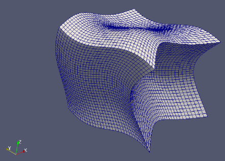
Figure 1: $3D$ Warped Grid

$$\begin{split}&x=\xi+\frac{1}{10}\Big{(}\cos{\pi\eta}+\cos{\pi\zeta}\Big{)},\\ &y=\eta+\frac{1}{10}\exp{(1-\eta)}\Big{(}\sin{\pi\xi}+\sin{\pi\zeta}\Big{)},\\ &z=\zeta+\frac{1}{20}(\sin{2\pi\xi}+\sin{2\pi\eta}),\\ &[\xi,\eta,\zeta]\in[0,1]^{3}.\end{split}$$ (64)

$$\begin{split}&\bm{f}=[\exp{(-10x^{2})},\exp{(-10\pi y^{3})},\exp{(-10\sin{z})}],\\ &\nabla\cdot\bm{f}_{\text{exact}}=-10\Big{(}2x\exp{(-10x^{2})}+3\pi y^{2}\exp{(-10\pi y^{3})}+\cos{(z)}\exp{(-10\sin{z})}\Big{)}.\end{split}$$ (65)

The maximum GCL computed for the grid was O(1e-15). First, we demonstrate in Tables 2 through 4 that the error levels change as we increase $c$, but the orders remain unchanged until $c\gg c_{+}$. Next, for the polynomial order range, $p=2$ through $p=5$, we verify that applying the ESFR filter operator does not affect the order of accuracy up to a certain value, and by Thm. 2, the scheme loses all orders of accuracy at this value. The black star is the location of $c_{+}$ in Figures 3 through 5. The drop off value of $c$ closely resembles the values obtained by Castonguay [7, Figure 3.6].

dx	$c_{DG}$	OOA	$c_{+}$	OOA
3.125e-02	1.949e-02	-	1.860e-02	-
1.563e-02	2.587e-03	2.91	2.467e-03	2.91
7.813e-03	3.285e-04	2.98	3.133e-04	2.98
3.906e-03	4.122e-05	2.99	3.931e-05	2.99

Table 1: $L_{2}$ Convergence Table $p=3$

dx	$c_{DG}$	OOA	$c_{+}$	OOA
3.125e-02	4.436e-01	-	3.713e-01	-
1.563e-02	7.033e-02	2.66	5.746e-02	2.69
7.813e-03	9.885e-03	2.83	8.056e-03	2.83
3.906e-03	1.309e-03	2.92	1.072e-03	2.91

Table 2: $L_{\infty}$ Convergence Table $p=3$

dx	$c_{DG}$	OOA	$c_{+}$	OOA
2.5000e-02	1.618e-03	-	1.559e-03	-
1.2500e-02	1.070e-04	3.92	1.032e-04	3.92
6.2500e-03	6.784e-06	3.98	6.542e-06	3.98
3.1250e-03	4.256e-07	3.99	4.103e-07	3.99

Table 3: $L_{2}$ Convergence Table $p=4$

dx	$c_{DG}$	OOA	$c_{+}$	OOA
2.5000e-02	4.648e-02	-	4.085e-02	-
1.2500e-02	3.388e-03	3.78	3.033e-03	3.75
6.2500e-03	2.296e-04	3.88	2.056e-04	3.88
3.1250e-03	1.496e-05	3.94	1.341e-05	3.94

Table 4: $L_{\infty}$ Convergence Table $p=4$

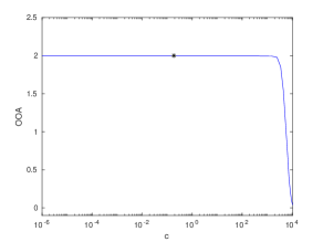
Figure 2: 3D $c$ vs OOA for $p=2$

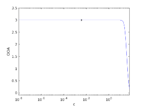
Figure 3: 3D $c$ vs OOA for $p=3$

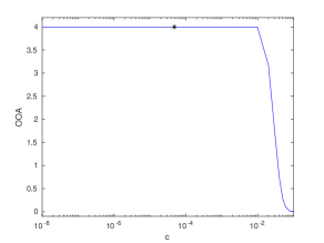
Figure 4: 3D $c$ vs OOA for $p=4$

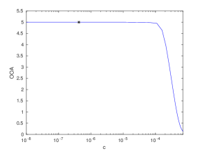
Figure 5: 3D $c$ vs OOA for $p=5$

7.2 Nonsymmetric Grid

As illustrated by Thm 1, the nonlinear metric terms vanish for both symmetric and skew-symmetric grids; resulting in a false-positive stable solution. Thus, a nonsymmetric grid was chosen to ensure that nonlinear metric terms are present. The warping for the nonsymmetric grid is similar to that used by Wu et al. [80], defined by Eq. (66), and the grid is illustrated in Fig. 6,

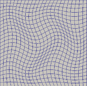
Figure 6: Warped Grid $p=3$

$$\begin{split}&x=\xi+\frac{1}{10}\cos{\frac{\pi}{2}\xi}\cos{\frac{3\pi}{2}\eta}\\ &y=\eta+\frac{1}{10}\sin{2\pi\xi}\cos{\frac{\pi}{2}\eta},\\ &[\xi,\eta]\in[-1,1]^{2}.\end{split}$$ (66)

We apply the following linear advection problem in Eq. (67),

$$\begin{split}\frac{\partial u}{\partial t}+1.1\frac{\partial u}{\partial x}-\frac{\pi}{e}\frac{\partial u}{\partial y}=0,\\ u(x,y,0)=e^{-20(x^{2}+y^{2})},\end{split}$$ (67)

with periodic boundary conditions. We integrate with a Runge-Kutta-4 integrator, using a timestep $dt=0.05dx$, with $dx$ being the average distance between two quadrature nodes. The grid is partitioned into $8^{2}$ elements. All results are uncollocated, with the solution built on the GLL nodes and integrated on the GL nodes. Since our metrics were computed via Eq. (50) and surface splitting was used, we were able to use GL nodes for both volume and surface integration without any form of optimization seen in the literature [40]. We first show energy results for uncollocated integration in Table 5, then uncollocated overintegration in Table 6.

Scheme	Flux	Energy Conserved $\mathcal{O}$(1e-12)	Energy Monotonically Decrease
Cons. DG	Central	No	No
Cons. DG	Upwind	No	No
EFSR Split $c_{DG}$	Central	Yes	Yes
EFSR Split $c_{DG}$	Upwind	No	Yes
EFSR Split $c_{+}$	Central	Yes	Yes
EFSR Split $c_{+}$	Upwind	No	Yes
EFSR Classical Split $c_{+}$	Central	No	No
EFSR Classical Split $c_{+}$	Upwind	No	No

Table 5: Energy Results $p=3,4$ Uncollocated $N_{vp}=(p+1)^{2}$ Grid 1

Scheme	Flux	Energy Conserved $\mathcal{O}$(1e-12)	Energy Monotonically Decrease
Cons. DG	Central	No	No
Cons. DG	Upwind	No	No
EFSR Split $c_{DG}$	Central	Yes	Yes
EFSR Split $c_{DG}$	Upwind	No	Yes
EFSR Split $c_{+}$	Central	Yes	Yes
EFSR Split $c_{+}$	Upwind	No	Yes
EFSR Classical Split $c_{+}$	Central	No	No
EFSR Classical Split $c_{+}$	Upwind	No	No

Table 6: Energy Results $p=3,4$ Uncollocated $N_{vp}=(p+3)^{2}$ Grid 1

An interesting result in Tables 5 and 6 is the false positive for the ESFR Classical split with an upwind numerical flux. From the derivation of our proposed curvilinear FR schemes in Sec. 4.1, specifically Eq. (34), there is no stability claim for the two terms $\bm{K}_{m}\Big{(}\bm{J}_{m}^{-1}\nabla^{r}\bm{\chi}(\bm{\xi}_{v}^{r})\Big{)}$ and $\bm{K}_{m}\Big{(}\bm{J}_{m}^{-1}\tilde{\nabla}^{r}\bm{\chi}(\bm{\xi}_{v}^{r})\Big{)}$ as they can result in either a convergent or divergent scheme. The advantage of our proposed FR schemes is that they are provably stable. In the next test case, it will be shown that the ESFR classical split is divergent for a skew-symmetric grid.

To demonstrate the orders of accuracy, we consider the linear advection problem in Eq. (68),

$$\begin{split}\frac{\partial u}{\partial t}+\frac{\partial u}{\partial x}+\frac{\partial u}{\partial y}=0,\\ [x,y]\in[-1,1]^{2},\text{ }t\in[0,2]\\ u(x,y,0)=\sin{\pi x}\sin{\pi y},\\ u_{exact}(x,y,t)=\sin{\pi(x-t)}\sin{\pi(y-t)}.\end{split}$$ (68)

We used a timestep of $dt=0.5dx$, where again $dx$ is the average distance between two quadrature nodes. The convergence rates are shown in Tables 8 through 10 for uncollocated integration, and Tables 12 through 14 for uncollocated overintegration.

dx	$c_{DG}$	OOA	$c_{+}$	OOA
6.2500e-02	1.4592e-02	-	3.9628e-02	-
3.1250e-02	1.1632e-03	3.65	3.0945e-03	3.68
1.5625e-02	7.4833e-05	3.96	1.7779e-04	4.12
7.8125e-03	4.7374e-06	3.98	1.0851e-05	4.03
3.9062e-03	3.0227e-07	3.97	6.8311e-07	3.99

Table 7: $L_{2}$ Convergence Table $p=3$ $N_{vp}=(p+1)^{2}$ Upwind Numerical Flux Grid 1

dx	$c_{DG}$	OOA	$c_{+}$	OOA
6.2500e-02	4.7490e-02	-	1.1192e-01	-
3.1250e-02	5.2854e-03	3.17	1.4510e-02	2.95
1.5625e-02	3.6961e-04	3.84	1.5445e-03	3.23
7.8125e-03	2.5181e-05	3.88	8.0837e-05	4.26
3.9062e-03	1.6401e-06	3.94	5.2672e-06	3.94

Table 8: $L_{\infty}$ Convergence Table $p=3$ $N_{vp}=(p+1)^{2}$ Upwind Numerical Flux Grid 1

dx	$c_{DG}$	OOA	$c_{+}$	OOA
5.0000e-02	3.7766e-03	-	8.1107e-03	-
2.5000e-02	1.4876e-04	4.67	2.5675e-04	4.98
1.2500e-02	5.1042e-06	4.87	9.2869e-06	4.79
6.2500e-03	1.6763e-07	4.93	3.1350e-07	4.89
3.1250e-03	5.4776e-09	4.94	1.0345e-08	4.92

Table 9: $L_{2}$ Convergence Table $p=4$ $N_{vp}=(p+1)^{2}$ Upwind Numerical Flux Grid 1

dx	$c_{DG}$	OOA	$c_{+}$	OOA
5.0000e-02	1.7943e-02	-	3.4934e-02	-
2.5000e-02	7.1420e-04	4.65	1.8378e-03	4.25
1.2500e-02	2.7883e-05	4.67	6.7414e-05	4.77
6.2500e-03	1.0551e-06	4.72	2.9290e-06	4.52
3.1250e-03	3.4989e-08	4.91	1.0435e-07	4.81

Table 10: $L_{\infty}$ Convergence Table $p=4$ $N_{vp}=(p+1)^{2}$ Upwind Numerical Flux Grid 1

dx	$c_{DG}$	OOA	$c_{+}$	OOA
6.2500e-02	1.4539e-02	-	3.9565e-02	-
3.1250e-02	1.1594e-03	3.65	3.0883e-03	3.68
1.5625e-02	7.4762e-05	3.95	1.7771e-04	4.12
7.8125e-03	4.7363e-06	3.98	1.0849e-05	4.03
3.9062e-03	3.0074e-07	3.98	6.8243e-07	3.99

Table 11: $L_{2}$ Convergence Table $p=3$ $N_{vp}=(p+3)^{2}$ Upwind Numerical Flux Grid 1

dx	$c_{DG}$	OOA	$c_{+}$	OOA
6.2500e-02	4.7467e-02	-	1.1172e-01	-
3.1250e-02	5.2245e-03	3.18	1.4400e-02	2.96
1.5625e-02	3.6902e-04	3.82	1.5435e-03	3.22
7.8125e-03	2.5167e-05	3.87	8.0826e-05	4.26
3.9062e-03	1.6398e-06	3.94	5.2670e-06	3.94

Table 12: $L_{\infty}$ Convergence Table $p=3$ $N_{vp}=(p+3)^{2}$ Upwind Numerical Flux Grid 1

dx	$c_{DG}$	OOA	$c_{+}$	OOA
5.0000e-02	3.7361e-03	-	8.0479e-03	-
2.5000e-02	1.4812e-04	4.66	2.5660e-04	4.97
1.2500e-02	5.0980e-06	4.86	9.2793e-06	4.79
6.2500e-03	1.6758e-07	4.93	3.1344e-07	4.89
3.1250e-03	5.4642e-09	4.94	1.0338e-08	4.92

Table 13: $L_{2}$ Convergence Table $p=4$ $N_{vp}=(p+3)^{2}$ Upwind Numerical Flux Grid 1

dx	$c_{DG}$	OOA	$c_{+}$	OOA
5.0000e-02	1.7408e-02	-	3.4462e-02	-
2.5000e-02	7.0797e-04	4.62	1.8335e-03	4.23
1.2500e-02	2.7798e-05	4.67	6.7391e-05	4.77
6.2500e-03	1.0549e-06	4.72	2.9288e-06	4.52
3.1250e-03	3.4983e-08	4.91	1.0434e-07	4.81

Table 14: $L_{\infty}$ Convergence Table $p=4$ $N_{vp}=(p+3)^{2}$ Upwind Numerical Flux Grid 1

7.3 Skew-Symmetric Grid

For further verification, we conduct the same experiments on the skew-symmetric grid from Hennemann et al. [81], shown in Fig.7, with warping defined in Eq. (69),

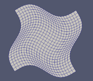
Figure 7: Second Warped Grid $p=3$

$$\begin{split}&x=\xi-0.1\sin{2\pi\eta},\\ &y=\eta+0.1\sin{2\pi\xi},\\ &[\xi,\eta]\in[0,1]^{2}.\end{split}$$ (69)

The sole purpose of using a skew-symmetric grid, is to show that even in the case when the grid has all the nonlinear metric terms cancel out, as per Thm. 1, Remark 2 holds because the determinant of the metric Jacobian cannot be factored out of the $\partial^{(s,v,w)}$ derivative. Thus, the ESFR correction functions must satisfy the metric dependent stability criteria in Eq. (36). We use the same initial condition described in Eq. (67) for the energy results, presented in Tables 15 and 16.

Scheme	Flux	Energy Conserved $\mathcal{O}$(1e-12)	Energy Monotonically Decrease
Cons. DG	Central	Yes	Yes
Cons. DG	Upwind	No	Yes
EFSR Split $c_{DG}$	Central	Yes	Yes
EFSR Split $c_{DG}$	Upwind	No	Yes
EFSR Split $c_{+}$	Central	Yes	Yes
EFSR Split $c_{+}$	Upwind	No	Yes
EFSR Classical Split $c_{+}$	Central	No	No
EFSR Classical Split $c_{+}$	Upwind	No	No

Table 15: Energy Results $p=3,4$ Uncollocated $N_{vp}=(p+1)^{2}$ Grid 2

Scheme	Flux	Energy Conserved $\mathcal{O}$(1e-12)	Energy Monotonically Decrease
Cons. DG	Central	Yes	Yes
Cons. DG	Upwind	No	Yes
EFSR Split $c_{DG}$	Central	Yes	Yes
EFSR Split $c_{DG}$	Upwind	No	Yes
EFSR Split $c_{+}$	Central	Yes	Yes
EFSR Split $c_{+}$	Upwind	No	Yes
EFSR Classical Split $c_{+}$	Central	No	No
EFSR Classical Split $c_{+}$	Upwind	No	No

Table 16: Energy Results $p=3,4$ Uncollocated $N_{vp}=(p+3)^{2}$ Grid 2

An interesting result from this grid is that conservative DG without the split form was stable, due to the skew-symmetry of the grid; while, ESFR classical split form was unstable. This highlights the importance of false positives while testing curvilinear grids. To demonstrate the orders of accuracy, we consider the linear advection problem from Eq. (68), and present the results in Tables 18 to 24.

dx	$c_{DG}$	OOA	$c_{+}$	OOA
6.2500e-02	6.9001e-03	-	2.2205e-02	-
3.1250e-02	4.9929e-04	3.79	2.1666e-03	3.36
1.5625e-02	3.0374e-05	4.04	9.5947e-05	4.50
7.8125e-03	1.9340e-06	3.97	5.6723e-06	4.08
3.9062e-03	1.2339e-07	3.97	3.5426e-07	4.00

Table 17: $L_{2}$ Convergence Table $p=3$ $N_{vp}=(p+1)^{2}$ Upwind Numerical Flux Grid 2

dx	$c_{DG}$	OOA	$c_{+}$	OOA
6.2500e-02	4.0068e-02	-	1.6836e-01	-
3.1250e-02	3.7121e-03	3.43	2.7181e-02	2.63
1.5625e-02	3.0497e-04	3.61	1.2679e-03	4.42
7.8125e-03	2.1527e-05	3.82	6.7106e-05	4.24
3.9062e-03	1.4001e-06	3.94	4.0344e-06	4.06

Table 18: $L_{\infty}$ Convergence Table $p=3$ $N_{vp}=(p+1)^{2}$ Upwind Numerical Flux Grid 2

dx	$c_{DG}$	OOA	$c_{+}$	OOA
5.0000e-02	1.5174e-03	-	3.7476e-03	-
2.5000e-02	4.8840e-05	4.96	1.0266e-04	5.19
1.2500e-02	1.6575e-06	4.88	3.7381e-06	4.78
6.2500e-03	5.9007e-08	4.81	1.4512e-07	4.69
3.1250e-03	2.1770e-09	4.76	5.2669e-09	4.78

Table 19: $L_{2}$ Convergence Table $p=4$ $N_{vp}=(p+1)^{2}$ Upwind Numerical Flux Grid 2

dx	$c_{DG}$	OOA	$c_{+}$	OOA
5.0000e-02	9.6178e-03	-	2.4719e-02	-
2.5000e-02	3.9077e-04	4.62	1.2826e-03	4.27
1.2500e-02	1.5061e-05	4.70	5.5561e-05	4.53
6.2500e-03	6.9115e-07	4.45	2.6736e-06	4.38
3.1250e-03	2.4981e-08	4.79	1.0379e-07	4.69

Table 20: $L_{\infty}$ Convergence Table $p=4$ $N_{vp}=(p+1)^{2}$ Upwind Numerical Flux Grid 2

dx	$c_{DG}$	OOA	$c_{+}$	OOA
6.2500e-02	6.8280e-03	-	2.2131e-02	-
3.1250e-02	4.9794e-04	3.78	2.1647e-03	3.35
1.5625e-02	3.0357e-05	4.04	9.5922e-05	4.50
7.8125e-03	1.9337e-06	3.97	5.6719e-06	4.08
3.9062e-03	1.2338e-07	3.97	3.5425e-07	4.00

Table 21: $L_{2}$ Convergence Table $p=3$ $N_{vp}=(p+3)^{2}$ Upwind Numerical Flux Grid 2

dx	$c_{DG}$	OOA	$c_{+}$	OOA
6.2500e-02	3.9689e-02	-	1.6899e-01	-
3.1250e-02	3.6977e-03	3.42	2.7110e-02	2.64
1.5625e-02	3.0464e-04	3.60	1.2676e-03	4.42
7.8125e-03	2.1521e-05	3.82	6.7102e-05	4.24
3.9062e-03	1.4000e-06	3.94	4.0343e-06	4.06

Table 22: $L_{\infty}$ Convergence Table $p=3$ $N_{vp}=(p+3)^{2}$ Upwind Numerical Flux Grid 2

dx	$c_{DG}$	OOA	$c_{+}$	OOA
5.0000e-02	1.5058e-03	-	3.7268e-03	-
2.5000e-02	4.8725e-05	4.95	1.0251e-04	5.18
1.2500e-02	1.6566e-06	4.88	3.7369e-06	4.78
6.2500e-03	5.8997e-08	4.81	1.4511e-07	4.69
3.1250e-03	2.1769e-09	4.76	5.2668e-09	4.78

Table 23: $L_{2}$ Convergence Table $p=4$ $N_{vp}=(p+3)^{2}$ Upwind Numerical Flux Grid 2

dx	$c_{DG}$	OOA	$c_{+}$	OOA
5.0000e-02	9.5289e-03	-	2.4636e-02	-
2.5000e-02	3.8874e-04	4.62	1.2817e-03	4.26
1.2500e-02	1.5046e-05	4.69	5.5551e-05	4.53
6.2500e-03	6.9098e-07	4.44	2.6735e-06	4.38
3.1250e-03	2.4979e-08	4.79	1.0379e-07	4.69

Table 24: $L_{\infty}$ Convergence Table $p=4$ $N_{vp}=(p+3)^{2}$ Upwind Numerical Flux Grid 2

8 Conclusion

This article proved that discrete integration by parts is not satisfied in the physical space for DG conservative and non-conservative forms, as well as standard FR forms, even with analytically exact metric terms and exact integration—provided that the basis functions are polynomial in the reference space. This lead to the formulation of metric dependent FR correction functions. Through the construction of metric dependent FR correction functions, the inclusion of metric Jacobian dependence within arbitrarily dense norms was derived and manifested through the FR broken Sobolev-norm. The resultant curvilinear expression had the correction functions filtering all modes of the discretization. The theoretical findings were numerically verified with a three-dimensional, heavily warped, non-symmetric grid, where the orders of convergence were lost at the equivalent correction parameter value $c$ as that of the one-dimensional ESFR scheme.

We derived dense, modal or nodal, FR schemes in curvilinear coordinates that ensured provable stability and conservation. This was achieved by incorporating the FR correction functions (FR filter operator) on both the volume and surface terms. Through a suite of curvilinear test-cases, one being non-symmetric and the other being skew-symmetric, the provable stability claim was numerically verified for our proposed FR schemes. The choice of grids highlighted the importance of assessing false-positives, especially in curvilinear coordinates where metric skew-symmetry has the metric cross-terms cancel out, as well as when metric symmetry combined with equivalent advection speeds in every physical direction results in an equivalence between the conservative and non-conservative forms. It was also numerically verified that FR schemes that solely use the correction functions to reconstruct the surface are divergent in general curvilinear coordinates—in both conservative and in split form. Lastly, we demonstrate that the proposed FR scheme retains optimal orders of accuracy in the appropriate range of $c$ values.

9 Acknowledgements

We would like to gratefully acknowledge the financial support of the Natural Sciences and Engineering Research Council of Canada Discovery Grant Program and McGill University. Jesse Chan acknowledges support from the US National Science Foundation under awards DMS-1719818 and DMS-1943186.

A Summation-by-Parts

The proposed algorithm in this paper is inspired by developments in the SBP literature, but derived using standard techniques and arguments from both the DG and FR communities. In this section, we make the link to the SBP formalism direct by assembling the relevant SBP operators.

The stiffness operators satisfy discrete integration by parts for quadrature rules of at least $2p-1$ strength,

$$\begin{split}\int_{\bm{\Omega}_{r}}\chi_{i}(\bm{\xi}^{r})\nabla^{r}\chi_{j}(\bm{\xi}^{r})d\bm{\Omega}_{r}+\int_{\bm{\Omega}_{r}}\nabla^{r}\chi_{i}(\bm{\xi}^{r})\chi_{j}(\bm{\xi}^{r})d\bm{\Omega}_{r}=\int_{\bm{\Gamma}_{r}}\chi_{i}(\bm{\xi}^{r})\chi_{j}(\bm{\xi}^{r})\hat{\bm{n}}^{r}d\bm{\Gamma}_{r}\\ \Leftrightarrow\bm{\chi}(\bm{\xi}_{v}^{r})^{T}\bm{W}\nabla^{r}\bm{\chi}(\bm{\xi}_{v}^{r})+\nabla^{r}\bm{\chi}(\bm{\xi}_{v}^{r})^{T}\bm{W}\bm{\chi}(\bm{\xi}_{v}^{r})=\sum_{f=1}^{N_{f}}\sum_{k=1}^{N_{fp}}\bm{\chi}(\bm{\xi}_{f,k}^{r})^{T}W_{f,k}\hat{\bm{n}}^{r}\bm{\chi}(\bm{\xi}_{f,k}^{r}).\end{split}$$ (70)

A.1 SBP - Strong Form FR Split

We introduce the lifting operator,

$$\bm{L}_{q}=\bm{M}^{-1}\sum_{f=1}^{N_{f}}\bm{\chi}(\bm{\xi}_{f}^{r})^{T}\bm{W}_{f},$$ (71)

where $\bm{\chi}(\bm{\xi}_{f}^{r})$ stores the basis functions evaluated at all facet cubature nodes on the face $f$, and $\bm{W}_{f}$ is a diagonal matrix storing the quadrature weights on the face $f$.

We now introduce the SBP operator [73],

$$\bm{Q}^{i}=\bm{W}(\bm{M}^{-1}\bm{S}_{\xi})\bm{\Pi},$$

to formulate the skew-hybridized SBP operator from Chan [73, Eq. (10)],

$$\tilde{\bm{Q}}_{p}^{i}=\frac{1}{2}\begin{bmatrix}\bm{Q}^{i}-(\bm{Q}^{i})^{T}&\bm{W}\bm{\chi}(\bm{\xi}_{v}^{r})\bm{L}_{q}\operatorname{diag}(\hat{\bm{n}}_{f}^{\xi})\\ -\sum_{f=1}^{N_{f}}\bm{W}_{f}\operatorname{diag}(\hat{\bm{n}}_{f}^{\xi})\bm{\chi}(\bm{\xi}_{f}^{r})\bm{\Pi}&\sum_{f=1}^{N_{f}}\bm{W}_{f}\operatorname{diag}(\hat{\bm{n}}_{f}^{\xi})\end{bmatrix}.$$ (72)

Next, similar to Chan [73, Eq. (27)], we introduce the metric dependent hybridized SBP operator as,

$$\bm{Q}_{m}^{i}=\frac{1}{2}\sum_{j=1}^{d}\Big{(}\operatorname{diag}{\begin{bmatrix}\bm{C}_{m}(\bm{\xi}_{v}^{r})_{ji}\\ \bm{C}_{m}(\bm{\xi}_{f}^{r})_{ji}\end{bmatrix}}\tilde{\bm{Q}}_{p}^{j}+\tilde{\bm{Q}}_{p}^{j}\operatorname{diag}{\begin{bmatrix}\bm{C}_{m}(\bm{\xi}_{v}^{r})_{ji}\\ \bm{C}_{m}(\bm{\xi}_{f}^{r})_{ji}\end{bmatrix}}\Big{)}.$$ (73)

In equivalent form, we express Eq. (43) as,

$$\begin{split}\frac{d}{dt}\hat{\bm{u}}_{m}(t)^{T}+\Big{[}(\bm{M}_{m}+\bm{K}_{m})^{-1}\bm{\chi}(\bm{\xi}_{v}^{r})^{T}\>\>(\bm{M}_{m}+\bm{K}_{m})^{-1}\sum_{f=1}^{N_{f}}\bm{\chi}(\bm{\xi}_{f}^{r})^{T}\Big{]}\sum_{j=1}^{d}\Big{(}2\bm{Q}_{m}^{i}\circ\bm{F}^{j}_{S}\Big{)}\bm{1}^{T}\\ +\sum_{j=1}^{d}(\bm{M}_{m}+\bm{K}_{m})^{-1}\sum_{f=1}^{N_{f}}\operatorname{diag}{(\bm{n}_{m,j})}(\bm{f}_{j}^{*}-\bm{f}_{j}(\tilde{\bm{u}_{m}}))=\bm{0}^{T}\\ (\bm{F}^{i}_{S})_{jk}=\bm{f}_{S}^{i}(\tilde{\bm{u}}_{j},\tilde{\bm{u}}_{k}),\>\forall 1\leq j+k\leq N_{vp}+N_{fp},\end{split}$$ (74)

where $\bm{n}_{m}=\hat{\bm{n}}^{r}\bm{C}_{m}^{T}$.

We would like to emphasize that incorporating the ESFR filter on the volume terms does not create a new ESFR differential operator, but instead is a modification on the norm that the DG volume is projected on. That is, we project both the volume and the surface terms to the $p$-th order broken Sobolev-space in the nonlinearly stable FR scheme, whereas in DG, the volume and surfaces are projected onto the $L_{2}$-space.

B Stability Proof - Operator Form

Here we present the stability proof from Sec. 6.3 in operator form. We start by applying the $(\bm{M}_{m}+\bm{K}_{m})$-norm, and we quickly see that it cancels off with its respective inverse,

$$\begin{split}&\hat{\bm{u}}_{m}(t)\Big{(}\bm{M}_{m}+\bm{K}_{m}\Big{)}\frac{d}{dt}\hat{\bm{u}}_{m}(t)^{T}\\ &=-\hat{\bm{u}}_{m}(t)\Big{(}\bm{M}_{m}+\bm{K}_{m}\Big{)}\Big{(}\bm{M}_{m}+\bm{K}_{m}\Big{)}^{-1}\sum_{i=1}^{d}\sum_{j=1}^{d}\bm{\chi}(\bm{\xi}_{v}^{r})^{T}\bm{W}\Big{(}a_{i}\frac{\partial\bm{\chi}(\bm{\xi}_{v}^{r})}{\partial\xi_{j}}\bm{\Pi}(J_{m}^{\Omega}\frac{\partial\xi_{j}}{\partial x_{i}})\bm{\chi}(\bm{\xi}_{v}^{r})\hat{\bm{u}}_{m}(t)^{T}+a_{i}(J_{m}^{\Omega}\frac{\partial\xi_{j}}{\partial x_{i}})\frac{\partial\bm{\chi}(\bm{\xi}_{v}^{r})}{\partial\xi_{j}}\bm{\Pi}\bm{\chi}(\bm{\xi}_{v}^{r})\hat{\bm{u}}_{m}(t)^{T}\Big{)}\\ &-\hat{\bm{u}}_{m}(t)\Big{(}\bm{M}_{m}+\bm{K}_{m}\Big{)}\Big{(}\bm{M}_{m}+\bm{K}_{m}\Big{)}^{-1}\sum_{f=1}^{N_{f}}\bm{\chi}(\bm{\xi}_{f}^{r})^{T}\bm{W}_{f}\operatorname{diag}(\hat{\bm{n}}_{f}^{r})\bm{f}_{m}^{{C,r}^{T}}.\end{split}$$ (75)

Next, consider the volume terms with respect to a single $(i,j)$-pairing, substitute $\frac{\partial\bm{\chi}(\bm{\xi}_{v}^{r})}{\partial\xi_{j}}=\bm{\chi}(\bm{\xi}_{v}^{r})\bm{M}^{-1}\bm{S}_{\xi,j}$, and swap the metric terms with the quadrature weights in the second volume term,

$$\begin{split}\hat{\bm{u}}_{m}(t)\bm{\chi}(\bm{\xi}_{v}^{r})^{T}\bm{W}\Big{(}a_{i}\frac{\partial\bm{\chi}(\bm{\xi}_{v}^{r})}{\partial\xi_{j}}\bm{\Pi}(J_{m}^{\Omega}\frac{\partial\xi_{j}}{\partial x_{i}})\bm{\chi}(\bm{\xi}_{v}^{r})\hat{\bm{u}}_{m}(t)^{T}+a_{i}(J_{m}^{\Omega}\frac{\partial\xi_{j}}{\partial x_{i}})\frac{\partial\bm{\chi}(\bm{\xi}_{v}^{r})}{\partial\xi_{j}}\bm{\Pi}\bm{\chi}(\bm{\xi}_{v}^{r})\hat{\bm{u}}_{m}(t)^{T}\Big{)}\\ =a_{i}\hat{\bm{u}}_{m}(t)\bm{\chi}(\bm{\xi}_{v}^{r})^{T}\bm{W}\bm{\chi}(\bm{\xi}_{v}^{r})\bm{M}^{-1}\bm{S}_{\xi,j}\bm{\Pi}(J_{m}^{\Omega}\frac{\partial\xi_{j}}{\partial x_{i}})\bm{\chi}(\bm{\xi}_{v}^{r})\hat{\bm{u}}_{m}(t)^{T}+a_{i}\hat{\bm{u}}_{m}(t)\bm{\chi}(\bm{\xi}_{v}^{r})^{T}(J_{m}^{\Omega}\frac{\partial\xi_{j}}{\partial x_{i}})\bm{W}\bm{\chi}(\bm{\xi}_{v}^{r})\bm{M}^{-1}\bm{S}_{\xi,j}\bm{\Pi}\bm{\chi}(\bm{\xi}_{v}^{r})\hat{\bm{u}}_{m}(t)^{T}.\end{split}$$ (76)

We continue by substituting $\bm{\Pi}^{T}=\bm{W}\bm{\chi}(\bm{\xi}_{v}^{r})\bm{M}^{-1},\text{ and }\bm{\Pi}\bm{\chi}(\bm{\xi}_{v}^{r})=\bm{M}^{-1}\bm{M}=\bm{I}$,

$$\begin{split}&=a_{i}\hat{\bm{u}}_{m}(t)\bm{\chi}(\bm{\xi}_{v}^{r})^{T}\bm{\Pi}^{T}\bm{S}_{\xi,j}\bm{\Pi}(J_{m}^{\Omega}\frac{\partial\xi_{j}}{\partial x_{i}})\bm{\chi}(\bm{\xi}_{v}^{r})\hat{\bm{u}}_{m}(t)^{T}+a_{i}\hat{\bm{u}}_{m}(t)\bm{\chi}(\bm{\xi}_{v}^{r})^{T}(J_{m}^{\Omega}\frac{\partial\xi_{j}}{\partial x_{i}})\bm{\Pi}^{T}\bm{S}_{\xi,j}\hat{\bm{u}}_{m}(t)^{T}\\ &=a_{i}\Big{(}\bm{\Pi}\bm{\chi}(\bm{\xi}_{v}^{r})\hat{\bm{u}}_{m}(t)^{T}\Big{)}^{T}\bm{S}_{\xi,j}\bm{\Pi}(J_{m}^{\Omega}\frac{\partial\xi_{j}}{\partial x_{i}})\bm{\chi}(\bm{\xi}_{v}^{r})\hat{\bm{u}}_{m}(t)^{T}+a_{i}\hat{\bm{u}}_{m}(t)\bm{\chi}(\bm{\xi}_{v}^{r})^{T}(J_{m}^{\Omega}\frac{\partial\xi_{j}}{\partial x_{i}})\bm{\Pi}^{T}\bm{S}_{\xi,j}\hat{\bm{u}}_{m}(t)^{T}.\end{split}$$ (77)

Lastly, we substitute $\bm{\Pi}\bm{\chi}(\bm{\xi}_{v}^{r})=\bm{M}^{-1}\bm{M}=\bm{I}$ once more and then perform integration-by-parts on the first stiffness matrix to arrive at,

$$\begin{split}&=-a_{i}\hat{\bm{u}}_{m}(t)\bm{S}_{\xi,j}^{T}\bm{\Pi}(J_{m}^{\Omega}\frac{\partial\xi_{j}}{\partial x_{i}})\bm{\chi}(\bm{\xi}_{v}^{r})\hat{\bm{u}}_{m}(t)^{T}+a_{i}\hat{\bm{u}}_{m}(t)\bm{\chi}(\bm{\xi}_{v}^{r})^{T}(J_{m}^{\Omega}\frac{\partial\xi_{j}}{\partial x_{i}})\bm{\Pi}^{T}\bm{S}_{\xi,j}\hat{\bm{u}}_{m}(t)^{T}+\sum_{f=1}^{N_{f}}a_{i}\hat{\bm{u}}_{m}(t)\bm{\chi}(\bm{\xi}_{f}^{r})^{T}\operatorname{diag}(\hat{\bm{n}}^{\xi_{j}})\bm{\chi}(\bm{\xi}_{f})\hat{\bm{u}}_{m}(t)^{T}.\end{split}$$ (78)

The two volume terms are the transpose of each other, thus they cancel out and the resultant stability claim is the same as Eq. (62) in Sec. 6.3. ∎

References

- Huynh [2007] H. T. Huynh, A Flux Reconstruction Approach to High-Order Schemes Including Discontinuous Galerkin Methods, American Institute of Aeronautics and Astronautics, 2007. doi:10.2514/6.2007-4079.
- Wang and Gao [2009] Z. J. Wang, H. Gao, A unifying lifting collocation penalty formulation including the discontinuous Galerkin, spectral volume/difference methods for conservation laws on mixed grids, Journal of Computational Physics 228 (2009) 8161–8186.
- Huynh et al. [2014] H. Huynh, Z. J. Wang, P. E. Vincent, High-order methods for computational fluid dynamics: A brief review of compact differential formulations on unstructured grids, Computers & fluids 98 (2014) 209–220.
- Vincent et al. [2011] P. Vincent, P. Castonguay, A. Jameson, Insights from von Neumann analysis of high-order flux reconstruction schemes, Journal of Computational Physics 230 (2011) 8134–8154.
- Williams and Jameson [2014] D. M. Williams, A. Jameson, Energy Stable Flux Reconstruction Schemes for Advection –Diffusion Problems on Tetrahedra, Journal of Scientific Computing 59 (2014) 721–759.
- Vincent et al. [2015] P. Vincent, A. Farrington, F. Witherden, A. Jameson, An extended range of stable-symmetric-conservative Flux Reconstruction correction functions, Computer Methods in Applied Mechanics and Engineering 296 (2015) 248–272.
- Castonguay [2012] P. Castonguay, High-order energy stable flux reconstruction schemes for fluid flow simulations on unstructured grids, Diss. Stanford University (2012).
- Castonguay et al. [2012] P. Castonguay, P. E. Vincent, A. Jameson, A New Class of High-Order Energy Stable Flux Reconstruction Schemes for Triangular Elements, Journal of Scientific Computing 51 (2012) 224–256.
- Del Rey Fernández et al. [2014] D. C. Del Rey Fernández, J. E. Hicken, D. W. Zingg, Review of summation-by-parts operators with simultaneous approximation terms for the numerical solution of partial differential equations, Computers & Fluids 95 (2014) 171–196.
- Svärd and Nordström [2014] M. Svärd, J. Nordström, Review of summation-by-parts schemes for initial–boundary-value problems, Journal of Computational Physics 268 (2014) 17–38.
- Del Rey Fernández et al. [2014] D. C. Del Rey Fernández, P. D. Boom, D. W. Zingg, A generalized framework for nodal first derivative summation-by-parts operators, Journal of Computational Physics 266 (2014) 214–239.
- Carpenter et al. [1994] M. H. Carpenter, D. Gottlieb, S. Abarbanel, Time-stable boundary conditions for finite-difference schemes solving hyperbolic systems: methodology and application to high-order compact schemes, Journal of Computational Physics 111 (1994) 220–236.
- Carpenter et al. [1999] M. H. Carpenter, J. Nordström, D. Gottlieb, A stable and conservative interface treatment of arbitrary spatial accuracy, Journal of Computational Physics 148 (1999) 341–365.
- Nordström and Carpenter [1999] J. Nordström, M. H. Carpenter, Boundary and interface conditions for high-order finite-difference methods applied to the Euler and Navier–Stokes equations, Journal of Computational Physics 148 (1999) 621–645.
- Nordström and Carpenter [2001] J. Nordström, M. H. Carpenter, High-order finite difference methods, multidimensional linear problems, and curvilinear coordinates, Journal of Computational Physics 173 (2001) 149–174.
- Carpenter et al. [2010] M. H. Carpenter, J. Nordström, D. Gottlieb, Revisiting and extending interface penalties for multi-domain summation-by-parts operators, Journal of Scientific Computing 45 (2010) 118–150.
- Svärd and Özcan [2014] M. Svärd, H. Özcan, Entropy-stable schemes for the euler equations with far-field and wall boundary conditions, Journal of Scientific Computing 58 (2014) 61–89.
- Parsani et al. [2015a] M. Parsani, M. H. Carpenter, E. J. Nielsen, Entropy stable discontinuous interfaces coupling for the three-dimensional compressible Navier-Stokes equations., J. Comput. Phys. 290 (2015a) 132–138.
- Parsani et al. [2015b] M. Parsani, M. H. Carpenter, E. J. Nielsen, Entropy stable wall boundary conditions for the three-dimensional compressible Navier–Stokes equations, Journal of Computational Physics 292 (2015b) 88–113.
- Ranocha et al. [2016] H. Ranocha, P. Öffner, T. Sonar, Summation-by-parts operators for correction procedure via reconstruction, Journal of Computational Physics 311 (2016) 299–328.
- Ranocha et al. [2017] H. Ranocha, P. Öffner, T. Sonar, Extended skew-symmetric form for summation-by-parts operators and varying Jacobians, Journal of Computational Physics 342 (2017) 13–28.
- Montoya and Zingg [2021] T. Montoya, D. W. Zingg, A unifying algebraic framework for discontinuous galerkin and flux reconstruction methods based on the summation-by-parts property, arXiv preprint arXiv:2101.10478v1 (2021).
- Abgrall et al. [2019] R. Abgrall, P. Öffner, H. Ranocha, Reinterpretation and extension of entropy correction terms for residual distribution and discontinuous galerkin schemes, arXiv preprint arXiv:1908.04556 (2019).
- Abgrall [2018] R. Abgrall, A general framework to construct schemes satisfying additional conservation relations. application to entropy conservative and entropy dissipative schemes, Journal of Computational Physics 372 (2018) 640–666.
- Abgrall et al. [2018] R. Abgrall, E. l. Meledo, P. Oeffner, On the connection between residual distribution schemes and flux reconstruction, arXiv preprint arXiv:1807.01261 (2018).
- Abgrall et al. [2021] R. Abgrall, J. Nordström, P. Öffner, S. Tokareva, Analysis of the sbp-sat stabilization for finite element methods part ii: entropy stability, Communications on Applied Mathematics and Computation (2021) 1–23.
- Fisher [2012] T. C. Fisher, High-order L2 stable multi-domain finite difference method for compressible flows, Ph.D. thesis, Purdue University, 2012.
- Fisher et al. [2013] T. C. Fisher, M. H. Carpenter, J. Nordström, N. K. Yamaleev, C. Swanson, Discretely conservative finite-difference formulations for nonlinear conservation laws in split form: Theory and boundary conditions, Journal of Computational Physics 234 (2013) 353–375.
- Fisher and Carpenter [2013] T. C. Fisher, M. H. Carpenter, High-order entropy stable finite difference schemes for nonlinear conservation laws: Finite domains, Journal of Computational Physics 252 (2013) 518–557.
- Carpenter et al. [2014] M. H. Carpenter, T. C. Fisher, E. J. Nielsen, S. H. Frankel, Entropy stable spectral collocation schemes for the Navier–Stokes equations: Discontinuous interfaces, SIAM Journal on Scientific Computing 36 (2014) B835–B867.
- Parsani et al. [2016] M. Parsani, M. H. Carpenter, T. C. Fisher, E. J. Nielsen, Entropy stable staggered grid discontinuous spectral collocation methods of any order for the compressible Navier–Stokes equations, SIAM Journal on Scientific Computing 38 (2016) A3129–A3162.
- Carpenter et al. [2016] M. H. Carpenter, M. Parsani, E. J. Nielsen, T. C. Fisher, Towards an entropy stable spectral element framework for computational fluid dynamics, in: 54th AIAA Aerospace Sciences Meeting, 2016, p. 1058.
- Yamaleev and Carpenter [2017] N. K. Yamaleev, M. H. Carpenter, A family of fourth-order entropy stable nonoscillatory spectral collocation schemes for the 1-d Navier–Stokes equations, Journal of Computational Physics 331 (2017) 90–107.
- Crean et al. [2018] J. Crean, J. E. Hicken, D. C. Del Rey Fernández, D. W. Zingg, M. H. Carpenter, Entropy-stable summation-by-parts discretization of the Euler equations on general curved elements, Journal of Computational Physics 356 (2018) 410–438.
- Chen and Shu [2017] T. Chen, C.-W. Shu, Entropy stable high order discontinuous Galerkin methods with suitable quadrature rules for hyperbolic conservation laws, Journal of Computational Physics 345 (2017) 427–461.
- Crean et al. [2020] J. Crean, D. C. Del Rey Fernández, M. H. Carpenter, J. E. Hicken, Staggered entropy-stable summation-by- parts discretization of the Euler equations on general curved elements, accepted in Journal of Computational Physics (2020).
- Chan [2018] J. Chan, On discretely entropy conservative and entropy stable discontinuous Galerkin methods, Journal of Computational Physics 362 (2018) 346–374.
- Friedrich et al. [2020] L. Friedrich, G. Shnücke, A. R. Winters, D. C. Del Rey Fernández, G. J. Gassner, M. H. Carpenter, Entropy stable space-time discontinuous Galerkin schemes with summation-by-parts property for hyperbolic conservation, (Submitted to the Journal of Scientific Computing) (2020).
- Svärd [2004] M. Svärd, On coordinate transformations for summation-by-parts operators, Journal of Scientific Computing 20 (2004) 29–42.
- Fernández et al. [2019] D. C. D. R. Fernández, P. D. Boom, M. H. Carpenter, D. W. Zingg, Extension of tensor-product general- ized and dense-norm summation-by-parts operators to curvilinear coordinates, Journal of Scientific Computing 80 (2019) 1957–1996.
- Ålund and Nordström [2019] O. Ålund, J. Nordström, Encapsulated high order difference operators on curvilinear non-conforming grids, Journal of Computational Physics 385 (2019) 209–224.
- Wintermeyer et al. [2017] N. Wintermeyer, A. R. Winters, G. J. Gassner, D. A. Kopriva, An entropy stable nodal discontinuous Galerkin method for the two dimensional shallow water equations on unstructured curvilinear meshes with discontinuous bathymetry, Journal of Computational Physics 340 (2017) 200–242.
- Moxey et al. [2019] D. Moxey, S. P. Sastry, R. M. Kirby, Interpolation error bounds for curvilinear finite elements and their implications on adaptive mesh refinement, Journal of Scientific Computing 78 (2019) 1045–1062.
- Mengaldo et al. [2016] G. Mengaldo, D. De Grazia, P. E. Vincent, S. J. Sherwin, On the connections between discontinuous Galerkin and flux reconstruction schemes: extension to curvilinear meshes, Journal of Scientific Computing 67 (2016) 1272–1292.
- Jan S. Hesthaven [2008] T. W. Jan S. Hesthaven, Nodal Discontinuous Galerkin methods Algorithms, Analysis and Applications, Springer, 2008. doi:10.1007/978-0-387-72067-8.
- Karniadakis and Sherwin [2013] G. Karniadakis, S. Sherwin, Spectral/hp element methods for computational fluid dynamics, Oxford University Press, 2013.
- Zwanenburg and Nadarajah [2016] P. Zwanenburg, S. Nadarajah, Equivalence between the Energy Stable Flux Reconstruction and Filtered Discontinuous Galerkin Schemes, Journal of Computational Physics 306 (2016) 343–369.
- Teukolsky [2016] S. A. Teukolsky, Formulation of discontinuous Galerkin methods for relativistic astrophysics, Journal of Computational Physics 312 (2016) 333–356.
- Chan and Wilcox [2019] J. Chan, L. C. Wilcox, On discretely entropy stable weight-adjusted discontinuous Galerkin methods: curvilinear meshes, Journal of Computational Physics 378 (2019) 366–393.
- Vincent et al. [2011] P. E. Vincent, P. Castonguay, A. Jameson, A New Class of High-Order Energy Stable Flux Reconstruction Schemes, Journal of Scientific Computing 47 (2011) 50–72.
- Castonguay et al. [2012] P. Castonguay, P. E. Vincent, A. Jameson, A new class of high-order energy stable flux reconstruction schemes for triangular elements, Journal of Scientific Computing 51 (2012) 224–256.
- Cicchino and Nadarajah [2020] A. Cicchino, S. Nadarajah, A new norm and stability condition for tensor product flux reconstruction schemes, Journal of Computational Physics (2020) 110025.
- Abe et al. [2018] Y. Abe, I. Morinaka, T. Haga, T. Nonomura, H. Shibata, K. Miyaji, Stable, non-dissipative, and conservative flux-reconstruction schemes in split forms, Journal of Computational Physics 353 (2018) 193–227.
- De Grazia et al. [2014] D. De Grazia, G. Mengaldo, D. Moxey, P. Vincent, S. Sherwin, Connections between the discontinuous Galerkin method and high-order flux reconstruction schemes, International journal for numerical methods in fluids 75 (2014) 860–877.
- Gassner et al. [2016] G. J. Gassner, A. R. Winters, D. A. Kopriva, Split form nodal discontinuous galerkin schemes with summation-by-parts property for the compressible euler equations, Journal of Computational Physics 327 (2016) 39–66.
- Cicchino et al. [2021] A. Cicchino, S. Nadarajah, D. Del Rey Fernández, Nonlinearly stable flux reconstruction high-order methods in split form, (Submitted to the Journal of Computational Physics) (2021).
- Jameson et al. [2012] A. Jameson, P. E. Vincent, P. Castonguay, On the Non-linear Stability of Flux Reconstruction Schemes, Journal of Scientific Computing 50 (2012) 434–445.
- Castonguay et al. [2013] P. Castonguay, D. M. Williams, P. Vincent, A. Jameson, Energy stable flux reconstruction schemes for advection –diffusion problems, Computer Methods in Applied Mechanics and Engineering 267 (2013) 400–417.
- Sheshadri and Jameson [2016] A. Sheshadri, A. Jameson, On the stability of the flux reconstruction schemes on quadrilateral elements for the linear advection equation, Journal of Scientific Computing 67 (2016) 769–790.
- Allaneau and Jameson [2011] Y. Allaneau, A. Jameson, Connections between the filtered discontinuous Galerkin method and the flux reconstruction approach to high order discretizations, Computer Methods in Applied Mechanics and Engineering 200 (2011) 3628–3636.
- Gassner et al. [2018] G. J. Gassner, A. R. Winters, F. J. Hindenlang, D. A. Kopriva, The br1 scheme is stable for the compressible navier–stokes equations, Journal of Scientific Computing 77 (2018) 154–200.
- Manzanero et al. [2019] J. Manzanero, G. Rubio, D. A. Kopriva, E. Ferrer, E. Valero, Entropy-stable discontinuous Galerkin approximation with summation-by-parts property for the incompressible navier-stokes/cahn-hilliard system, arXiv preprint arXiv:1910.11252 (2019).
- Kopriva [2006] D. A. Kopriva, Metric identities and the discontinuous spectral element method on curvilinear meshes, Journal of Scientific Computing 26 (2006) 301.
- Thomas and Lombard [1979] P. D. Thomas, C. K. Lombard, Geometric conservation law and its application to flow computations on moving grids, AIAA journal 17 (1979) 1030–1037.
- Vinokur and Yee [2002] M. Vinokur, H. Yee, Extension of efficient low dissipation high order schemes for 3-d curvilinear moving grids, in: Frontiers of Computational Fluid Dynamics 2002, World Scientific, 2002, pp. 129–164.
- Kopriva et al. [2019] D. A. Kopriva, F. J. Hindenlang, T. Bolemann, G. J. Gassner, Free-stream preservation for curved geometrically non-conforming discontinuous Galerkin spectral elements, Journal of Scientific Computing 79 (2019) 1389–1408.
- Botti [2012] L. Botti, Influence of reference-to-physical frame mappings on approximation properties of discontinuous piecewise polynomial spaces, Journal of Scientific Computing 52 (2012) 675–703.
- Del Rey Fernández et al. [2019] D. Del Rey Fernández, M. H. Carpenter, L. Dalcin, L. Fredrich, D. Rojas, A. R. Winters, G. J. Gassner, S. Zampini, M. Parsani, Entropy stable p-nonconforming discretizations with the summation-by-parts property for the compressible euler equations, arXiv preprint arXiv:1909.12536 (2019).
- Jameson [2010a] A. Jameson, A Proof of the Stability of the Spectral Difference Method for All Orders of Accuracy, Journal of Scientific Computing 45 (2010a) 348–358.
- Jameson [2010b] A. Jameson, A proof of the stability of the spectral difference method for all orders of accuracy, Journal of Scientific Computing 45 (2010b) 348–358.
- Huynh [2009] H. T. Huynh, A Reconstruction Approach to High-Order Schemes Including Discontinuous Galerkin for Diffusion, American Institute of Aeronautics and Astronautics, 2009. doi:10.2514/6.2009-403.
- Witherden et al. [2016] F. Witherden, P. Vincent, A. Jameson, High-order flux reconstruction schemes, in: Handbook of numerical analysis, volume 17, Elsevier, 2016, pp. 227–263.
- Chan [2019] J. Chan, Skew-symmetric entropy stable modal discontinuous Galerkin formulations, Journal of Scientific Computing 81 (2019) 459–485.
- Witherden et al. [2014] F. D. Witherden, A. M. Farrington, P. E. Vincent, Pyfr: An open source framework for solving advection–diffusion type problems on streaming architectures using the flux reconstruction approach, Computer Physics Communications 185 (2014) 3028–3040.
- Witherden and Vincent [2014] F. D. Witherden, P. E. Vincent, An analysis of solution point coordinates for flux reconstruction schemes on triangular elements, Journal of Scientific Computing 61 (2014) 398–423.
- Abe et al. [2015] Y. Abe, T. Haga, T. Nonomura, K. Fujii, On the freestream preservation of high-order conservative flux-reconstruction schemes, Journal of Computational Physics 281 (2015) 28–54.
- Johnen et al. [2013] A. Johnen, J.-F. Remacle, C. Geuzaine, Geometrical validity of curvilinear finite elements, Journal of Computational Physics 233 (2013) 359–372.
- Turner et al. [2018] M. Turner, J. Peiró, D. Moxey, Curvilinear mesh generation using a variational framework, Computer-Aided Design 103 (2018) 73–91.
- Shi-Dong and Nadarajah [2021] D. Shi-Dong, S. Nadarajah, Full-space approach to aerodynamic shape optimization, Computers & Fluids (2021) 104843.
- Wu et al. [2021] X. Wu, E. J. Kubatko, J. Chan, High-order entropy stable discontinuous galerkin methods for the shallow water equations: curved triangular meshes and gpu acceleration, Computers & Mathematics with Applications 82 (2021) 179–199.
- Hennemann et al. [2021] S. Hennemann, A. M. Rueda-Ramírez, F. J. Hindenlang, G. J. Gassner, A provably entropy stable subcell shock capturing approach for high order split form DG for the compressible Euler equations, Journal of Computational Physics 426 (2021) 109935.