Evolutionary Clustering of Streaming Trajectories

Abstract.

The widespread deployment of smartphones and location-enabled, networked in-vehicle devices renders it increasingly feasible to collect streaming trajectory data of moving objects. The continuous clustering of such data can enable a variety of real-time services, such as identifying representative paths or common moving trends among objects in real-time. However, little attention has so far been given to the quality of clusters—for example, it is beneficial to smooth short-term fluctuations in clusters to achieve robustness to exceptional data.

We propose the notion of evolutionary clustering of streaming trajectories, abbreviated ECO, that enhances streaming-trajectory clustering quality by means of temporal smoothing that prevents abrupt changes in clusters across successive timestamps. Employing the notions of snapshot and historical trajectory costs, we formalize ECO and then formulate ECO as an optimization problem and prove that ECO can be performed approximately in linear time, thus eliminating the iterative processes employed in previous studies. Further, we propose a minimal-group structure and a seed point shifting strategy to facilitate temporal smoothing. Finally, we present all algorithms underlying ECO along with a set of optimization techniques. Extensive experiments with two real-life datasets offer insight into ECO and show that it outperforms state-of-the-art solutions in terms of both clustering quality and efficiency.

1. Introduction

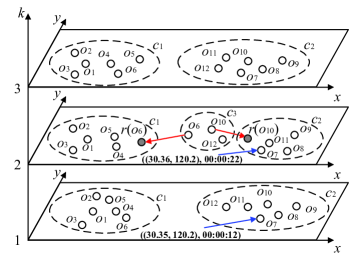
Figure 1. Motivating example

It is increasingly possible to equip moving objects with positioning devices that are capable of transmitting object positions to a central location in real time. Examples include people with smartphones and vehicles with built-in navigation devices or tracking devices. This scenario opens new opportunities for the real-time discovery of hidden mobility patterns. These patterns allow characterizing individual mobility for a certain time interval and enable a broad range of important services and applications such as route planning (Zeng et al., 2019; Wang et al., 2020), intelligent transportation management (Wang et al., 2021), and road infrastructure optimization (Wu et al., 2015).

As a typical moving pattern discovery approach, clustering aims to group a set of trajectories into comparatively homogeneous clusters to extract representative paths or movement patterns shared by moving objects. Considering a streaming setting, many works are proposed to cluster the trajectories in real-time (Jensen et al., 2007; Li et al., 2010; Yu et al., 2013b; Costa et al., 2014; Deng et al., 2015; Da Silva et al., 2016; Chen et al., 2019; Tang et al., 2012; Li et al., 2012). However, existing real-time clustering methods focus on the most current data, achieving low computational cost at the expense of clustering quality (Xu et al., 2014). In streaming settings, clusterings should be robust to short-term fluctuations in the underlying trajectory data, which may be achieved by means of smoothing (Chi et al., 2007). An example illustrates this.

Example 1.

Figure 1 shows the trajectories of 12 moving objects at three timestamps, $k=1,2,3$. Traditional clustering algorithms return the two clusters $c_{1}=\{o_{1},o_{2},o_{3},o_{4},o_{5},o_{6}\}$ and $c_{2}=\{o_{7},o_{8},o_{9},o_{10},o_{11},$
$o_{12}\}$ at the first timestamp, the three clusters $c_{1}=\{o_{1},o_{2},o_{3},o_{4},o_{5}\}$, $c_{2}=\{o_{7},o_{8},o_{9},o_{11}\}$, and $c_{3}=\{o_{6},o_{10},o_{12}\}$ at the second timestamp, and the same two clusters at the third timestamp as at the first timestamp.

The underlying reason for this result is the unusual behavior of objects $o_{6}$ and $o_{10}$ at the second timestamp. Clearly, returning the same two stable clusters for all three timestamps is a more robust and better-quality result. A naive approach to eliminating the effect of the two objects’ unusual behavior is to perform cleaning before clustering. However, studies of on two real-life datasets show that among the trajectories that cause the mutations of clusterings, 88.9% and 75.9% of the trajectories follow the speed constraint, while 97.8% and 96.1% of them are categorized as inliers (Ester et al., 1996). Moreover, in real-time applications, it is impractical to correct previous clusterings retroactively. Hence, it is difficult for existing cleaning techniques to facilitate smoothly shifted clustering sequences (Li et al., 2020a; Patil et al., 2018; Idrissov and Nascimento, 2012).

However, this problem can be addressed by applying evolutionary clustering (Kim and Han, 2009; Fenn et al., 2009; Chen et al., 2020; Chakrabarti et al., 2006; Chi et al., 2007; Gupta et al., 2011; Xu et al., 2014; Yin et al., 2021; Ma and Dong, 2017; Liu et al., 2020), where a good current clustering result is one that fits the current data well, while not deviating too much from the recent history of clusterings. Specifically, temporal smoothness is integrated into the measure of clustering quality (Chi et al., 2007). This way, evolutionary clustering is able to outperform traditional clustering as it can reflect long term trends while being robust to short-term variability. Put differently, applying evolutionary clustering to trajectories can mitigate adverse effects of intermittent noise on clustering and present users with smooth and consistent movement patterns. In Example 1, clustering with temporal consistency is obtained if $o_{6}$ is smoothed to $r(o_{6})$ and $o_{10}$ is smoothed to $r(o_{10})$ at the second timestamp. Motivated by this, we study evolutionary clustering of trajectories.

Existing evolutionary clustering studies target dynamic networks and are not suitable for trajectory applications, mainly for three reasons. First, the solutions are designed specifically for dynamic networks, which differ substantially from two-dimensional trajectory data. Second, the movement in trajectories is generally much faster than the evolution of dynamic networks, which renders the temporal smoothness used in existing studies too ”strict” for trajectories. Third, existing studies often optimize the clustering quality iteratively at each timestamp (Kim and Han, 2009; Chakrabarti et al., 2006; Yin et al., 2021; Folino and Pizzuti, 2013; Liu et al., 2020, 2019), which is computationally costly and is infeasible for large-scale trajectories.

We propose an efficient and effective method for evolutionary clustering of streaming trajectories (ECO). First, we adopt the idea of neighbor-based smoothing (Kim and Han, 2009) and develop a structure called minimal group that is summarized by a seed point in order to facilitate smoothing. Second, following existing studies (Chakrabarti et al., 2006; Yin et al., 2021; Xu et al., 2014; Folino and Pizzuti, 2013; Liu et al., 2020, 2019), we formulate ECO as an optimization problem that employs the new notions of snapshot cost and historical cost. The snapshot cost evaluates the true concept shift of clustering defined according to the distances between smoothed and original locations. The historical cost evaluates the temporal distance between locations at adjacent timestamps by the degree of closeness. Next, we prove that the proposed optimization function can be decomposed and that each component can be solved approximately in constant time. The effectiveness of smoothing is further improved by a seed point shifting strategy. Finally, we introduce a grid index structure and present algorithms for each component of evolutionary clustering along with a set of optimization techniques, to improve clustering performance. The paper’s main contributions are summarized as follows,

• We formalize ECO problem. To the best of our knowledge, this is the first proposal for streaming trajectory clustering that takes into account temporal smoothness.

• We formulate ECO as an optimization problem, based on the new notions of snapshot cost and historical cost. We prove that the optimization problem can be solved approximately in linear time.

• We propose a minimal group structure to facilitate temporal smoothing and a seed point shifting strategy to improve clustering quality of evolutionary clustering. Moreover, we present all algorithms needed to enable evolutionary clustering, along with a set of optimization techniques.

• Extensive experiments on two real-life datasets show that ECO advances the state-of-the-arts in terms of both clustering quality and efficiency.

The rest of paper is organized as follows. We present preliminaries in Section 2. We formulate the problem in Section 3 and derive its solution in Section 4. Section 5 presents the algorithms and optimization techniques. Section 6 covers the experimental study. Section 7 reviews related work, and Section 8 concludes and offers directions for future work.

2. Preliminaries

Table 1. Frequently used notation

Notation	Description
$o$	A trajectory
$\textit{dt}_{k}$	The $k^{th}$ time step
$o.l_{k}$, $o.t_{k}$	The location and timestamp of $o$ at $\textit{dt}_{k}$
$o.l$, $o.t$	A simplification of $o.l_{k}$, $o.t_{k}$ at $\textit{dt}_{k}$
$o.\tilde{l}$, $o.\tilde{t}$	A simplification of $o.l_{k-1}$, $o.t_{k-1}$ at $\textit{dt}_{k}$
$\mathcal{O}_{k}$	A set of trajectories at $\textit{dt}_{k}$
$r(o)$	An adjustment of $o.l$
$\mathcal{R}_{k}$	The set of adjustments of $\mathcal{O}_{k}$
$s$	A seed point of $o$ at the current time step $\textit{dt}_{k}$
$\tilde{s}$	A seed point of $o$ at the previous time step $\textit{dt}_{k-1}$
$\mathcal{S}_{k}$	The set of seed points at $\textit{dt}_{k}$
$\mathcal{M}_{k}(s)$	A minimal group summarized by a seed point $s$ at $\textit{dt}_{k}$
$\mathcal{SC}_{k}(r(o))$	The snapshot cost of a trajectory $o$ w.r.t. $r(o)$ at $\textit{dt}_{k}$
$\mathcal{TC}_{k}(r(o))$	The historical cost of a trajectory $o$ w.r.t. $r(o)$ at $\textit{dt}_{k}$
$c$	A cluster $c$
$\mathcal{C}_{k}$	The set of clusters obtained at $\textit{dt}_{k}$

2.1. Data Model

Definition 1.

A GPS record is a pair $(l,t)$, where $t$ is a timestamp and $l=(x,y)$ is the location, with $x$ being a longitude and $y$ being a latitude.

Definition 2.

A streaming trajectory $o$ is an unbounded ordered sequence of GPS records, $\langle(o.l_{1},o.t_{1}),(o.l_{2},o.t_{2})\cdots\rangle$.

The GPS records of a trajectory may be transmitted to a central location in an unsynchronized manner. To avoid this affecting the subsequent processing, we adopt an existing approach (Chen et al., 2019) and discretize time into short intervals that are indexed by integers. We then map the timestamp of each GPS record to the index of the interval that the timestamp belongs to. In particular, we assume that the start time is 00:00:00 UTC, and we partition time into intervals of duration $\Delta t=10s$. Then time series $\langle$00:00:01, 00:00:12, 00:00:20, 00:00:31, 00:00:44$\rangle$ and $\langle$00:00:00, 00:00:13, 00:00:21, 00:00:31, 00:00:40$\rangle$ are both mapped $\langle 0,1,2,3,4\rangle$. We call such a sequence a discretized time sequence and call each discretized timestamp a time step dt. We use trajectory and streaming trajectory interchangeably.

Definition 3.

A trajectory is active at time step $dt=[t_{1},t_{2}]$ if it contains a GPS record $(l,t)$ such that $t\in[t_{1},t_{2}]$.

Definition 4.

A snapshot $\mathcal{O}_{k}$ is the set of trajectories that are active at time step $\textit{dt}_{k}$.

Figure 1 shows three snapshots $\mathcal{O}_{1}$, $\mathcal{O}_{2}$, and $\mathcal{O}_{3}$, each of which contains twelve trajectories. Given the start time 00:00:00 and $\Delta t=10$, $(o_{7}.l,o_{7}.t)$ arrives at $\textit{dt}_{1}$ because 00:00:12 is mapped to 1. For simplicity, we use $o$ in figures to denote $o.l$. The interval duration $\Delta t$ is the default sample interval of the dataset. Since deviations between the default sample interval and the actual intervals are small (Li et al., 2020b), we can assume that each trajectory $o$ has at most one GPS record at each time step $\textit{dt}_{k}$. If this is not the case for a trajectory $o$, we simply keep $o$’s earliest GPS at the time step. This simplifies the subsequent clustering. Thus, the GPS record of $o$ at $\textit{dt}_{k}$ is denoted as $(o.l_{k},o.t_{k})$. If a trajectory $o$ is active at both $\textit{dt}_{k-1}$ and $\textit{dt}_{k}$ and the current time step is $\textit{dt}_{k}$, $o.l_{k}$ and $o.t_{k}$ are simplified as $o.l$ and $o.t$, and $o.l_{k-1}$ and $o.t_{k-1}$ are simplified as $o.\tilde{l}$ and $o.\tilde{t}$. At time step $\textit{dt}_{2}$ ($k=2$) in Figure 1, $o_{7}.\tilde{l}=o_{7}.{l}_{1}=(30.35,120.2)$, $o_{7}.\tilde{t}=o_{7}.{t}_{1}=\,\,$00:00:12, $o_{7}.l=o_{7}.{l}_{2}=(30.36,120.2)$, and $o_{7}.t=o_{7}.{t}_{2}=\,\,$00:00:22.

Definition 5.

A $\bm{\theta}$-neighbor set of a streaming trajectory $o\,(\in\mathcal{O}_{k})$ at the time step $\textit{dt}_{k}$ is $\mathcal{N}_{\theta}(o)=\{o^{\prime}|o^{\prime}\in\mathcal{O}_{k}\wedge d(o.l,o^{\prime}.l)\leq\theta\}$,where $d(\cdot)$ is Euclidean distance and $\theta$ is a distance threshold. $\lvert\mathcal{N}_{\theta}(o)\rvert$ is called the local density of $o$ w.r.t. ${\theta}$ at $\textit{dt}_{k}$.

Figure 2 plots $o_{i}\,(1\leq 1\leq 6)$ at $\textit{dt}_{1}$ from Figure 1, where $\mathcal{N}_{\delta}(o_{1})=\{o_{1},o_{2},o_{3}\}$.

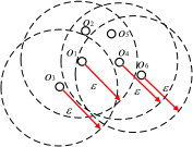
(a) Core points $o_{i}$ ($1\leq i\leq 6\wedge i\neq 3$) ($\textit{minPts}=3)$

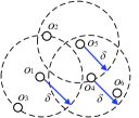
(b) Seed points $o_{1}$ and $o_{4}$ $(\rho=3)$

Figure 2. ${o_{i}\,(1\leq i\leq 6)}$ at ${\textit{dt}_{1}}$ in Figure 1

2.2. DBSCAN

We adopt a well-known density-based clustering approach, DBSCAN (Ester et al., 1996), for clustering. DBSCAN relies on two parameters to characterize density or sparsity, i.e., positive values $\varepsilon$ and minPts.

Definition 6.

A trajectory $o\in\mathcal{O}_{k}$ is a core point w.r.t. $\varepsilon$ and minPts, if $\mathcal{N}_{\varepsilon}(o)\geq\textit{minPts}$.

Definition 7.

A trajectory $o\in\mathcal{O}_{k}$ is density reachable from another trajectory $o^{\prime}\in\mathcal{O}_{k}$, if a sequence of trajectories $o_{1},o_{2},\cdots o_{n}~{}(n\geq 2)$ exists such that (i) $o_{1}=o^{\prime}$ and $o_{n}=o$; (ii) $o_{w}~{}(1\leq w<n)$ are core points; and (iii) $d(o_{w},o_{w+1})\leq\varepsilon~{}(1\leq w<n)$.

Definition 8.

A trajectory $o\in\mathcal{O}_{k}$ is connected to another trajectory $o^{\prime}$ if a trajectory $o^{\prime\prime}$ exists such that both $o$ and $o^{\prime}$ are density reachable from $o^{\prime\prime}$.

Definition 9.

A non-empty subset of trajectories of $\mathcal{O}_{k}$ is called a cluster $c$, if $c$ satisfies the following conditions:

• Connectivity: $\forall o,o^{\prime}\in c$, $o$ is connected to $o^{\prime}$;

• Maximality: $\forall o,o^{\prime}\in\mathcal{O}_{k}$, if $o\in c$ and $o^{\prime}$ is density reachable from $o$, then $o^{\prime}\in c$.

Definition 9 indicates that a cluster is formed by a set of core points and their density reachable points. Given $\varepsilon$ and minPts, $o\in\mathcal{O}_{k}$ is an outlier, if it is not in any cluster; $o\in\mathcal{O}_{k}$ is a border point, if $\mathcal{N}_{\varepsilon}(o)<\textit{minPts}$ and $d(o,o^{\prime})\leq\epsilon$, where $o^{\prime}$ is a core point.

Definition 10.

A clustering result $\mathcal{C}_{k}=\{c_{1},c_{2},\cdots,c_{n}\}$ is a set of clusters obtained from the snapshot $\mathcal{O}_{k}$.

Example 2.

In Figure 1, $\mathcal{C}_{1}$ has two clusters $c_{1}=\{o_{1},o_{2},o_{3},o_{4},o_{5},$
$o_{6}\}$ and $c_{2}=\{o_{7},o_{8},o_{9},o_{10},o_{11},o_{12}\}$. Further, $o_{i}$ ($1\leq i\leq 6\wedge i\neq 3$) in Figure 2a are core points.

2.3. Evolutionary Clustering

Evolutionary clustering is the problem producing a sequence of clusterings from streaming data; that is, clustering for each snapshot. It takes into account the smoothness characteristics of streaming data to obtain high-quality clusterings (Chakrabarti et al., 2006). Specifically, two quality aspects are considered:

• High historical quality: clustering $\mathcal{C}_{k}$ should be similar to the previous clustering $\mathcal{C}_{k-1}$;

• High snapshot quality: $\mathcal{C}_{k}$ should reflect the true concept shift of clustering, i.e., remain faithful to the data at each time step.

Evolutionary clustering uses a cost function $\mathcal{F}_{k}$ that enables trade-offs between historical quality and snapshot quality at each time step $\textit{dt}_{k}$ (Chakrabarti et al., 2006),

(1) $$\mathcal{F}_{k}=\mathcal{SC}_{k}(\mathcal{C}_{o},\mathcal{C}_{k})+\alpha\cdot\mathcal{TC}_{k}(\mathcal{C}_{k-1},\mathcal{C}_{k})$$

$\mathcal{F}_{k}$ is the sum of two terms: a snapshot cost ($\mathcal{SC}_{k}$) and a historical cost ($\mathcal{TC}_{k}$). The snapshot cost $\mathcal{SC}_{k}$ captures the similarity between clustering $\mathcal{C}_{k}$ and clustering $\mathcal{C}_{o}$ that is obtained without smoothing. The smaller $\mathcal{SC}_{k}$ is, the better the snapshot quality is. The historical cost $\mathcal{TC}_{k}$ measures how similar clustering $\mathcal{C}_{k}$ and the previous clustering $\mathcal{C}_{k-1}$ are. The smaller $\mathcal{TC}_{k}$ is, the better the historical quality is. Parameter $\alpha\,(>0)$ enables controlling the trades-off between snapshot quality and historical quality.

3. Problem Statement

We start by presenting two observations, based on which, we define the problem of evolutionary clustering of streaming trajectories.

3.1. Observations

Gradual evolutions of travel companions

As pointed out in a previous study (Tang et al., 2012), movement trajectories represent continuous and gradual location changes, rather than abrupt changes, implying that co-movements among trajectories also change only gradually over time. Co-movement may be caused by (i) physical constraints of both road networks and vehicles, and vehicles may have close relationships, e.g., they may belong to the same fleet or may target the same general destination (Tang et al., 2012).

Uncertainty of ”border” points

Even with the observation that movements captured by trajectories are not dramatic during a short time, border points are relatively more likely to leave their current cluster at the next time step than core points. This is validated by statistics from two real-life datasets. Specifically, among the trajectories shifting to another cluster or becoming an outlier during the next time steps, 75.0% and 61.5% are border points in the two real-life datasets.

3.2. Problem Definition

Cost embedding

Existing evolutionary clustering studies generally perform temporal smoothing on the clustering result (Folino and Pizzuti, 2013; Chakrabarti et al., 2006; Chi et al., 2007; Yin et al., 2021). Specifically, they adjust $\mathcal{C}_{k}$ iteratively so as to minimize Formula 1, which incurs very high cost. We adopt cost embedding (Kim and Han, 2009), which pushes down the cost formula from the clustering result level to the data level, thus enabling flexible and efficient temporal smoothing. However, the existing cost embedding technique (Kim and Han, 2009) targets dynamic networks only. To apply cost embedding to trajectories, we propose a minimal group structure and snapshot and historical cost functions.

Snapshot cost $\bm{\mathcal{SC}_{k}}$

We first define the notion of an ”adjustment” of a trajectory.

Definition 11.

An adjustment $r_{k}(o)$ is a location of a trajectory $o$ obtained through smoothing at $\textit{dt}_{k}$. Here, $r_{k}(o)\neq r_{k}(o^{\prime})$ if $o\neq o^{\prime}$. The set of adjustments in $\mathcal{O}_{k}$ is denoted as $\mathcal{R}_{k}$.

We simplify $r_{k}(o)$ to $r(o)$ if the context is clear. In Figure 1, $r(o_{6})$ is an adjustment of $o_{6}$ at $\textit{dt}_{2}$. According to Formula 1, the snapshot cost measures how similar the current clustering result $\mathcal{C}_{k}$ is to the original clustering result $\mathcal{C}_{o}$. Since we adopt cost embedding that smooths trajectories at the data level, the snapshot cost of a trajectory $o$ w.r.t. its adjustment $r(o)$ at $\textit{dt}_{k}$ (denoted as $\mathcal{SC}_{k}(r(o))$) is formulated as the deviation between $o$ and $r(o)$ at $\textit{dt}_{k}$:

(2) $$\mathcal{SC}_{k}(r(o))=d(r(o),o.l)^{2}\quad s.t.\quad d(r(o),o.\tilde{l})\leq\mu\cdot(o.t-o.\tilde{t}),$$

where $\mu$ is a speed constraint of the road network. Formula 2 requires that any adjustment $r(o)$ must follow the speed constraint. Obviously, the larger the distance between $o.l$ and its adjustment $r(o)$, the higher the snapshot cost.

Historical cost $\bm{\mathcal{TC}_{k}}$

As discussed in Section 2.3, one of the goals of evolutionary clustering is smoothing the change of clustering results during adjacent time steps. Since we push down the smoothing from the cluster level to trajectory level, the problem becomes one of ensuring that each trajectory represents a smooth movement. According to the first observation in Section 3.1, gradual location changes lead to stable co-movement relationships among trajectories during short periods of time. Thus, similar to neighbor-based smoothing in dynamic communities (Kim and Han, 2009), it is reasonable to smooth the location of each trajectory in the current time step using its neighbours at the previous time step. However, the previous study (Kim and Han, 2009) smooths the distance between each pair of neighboring nodes. Simply applying this to trajectories may degrade the performance of smoothing if a ”border” point is involved. Recall the second observation of Section 3.1 and assume that $o_{1}.l$ is smoothed according to $o_{3}.l$ at $\textit{dt}_{2}$ in Figures 1 and 2 . As $o_{3}$ is a border point at $\textit{dt}_{1}$ with a higher probability to leave the cluster $c_{1}$ at $\textit{dt}_{2}$, using $o_{3}$ to smooth $o_{1}$ may result in $o_{1}$ also leaving $c_{1}$ or being located at the border of $c_{1}$ at $\textit{dt}_{2}$. The first case may incur an abrupt change to the clustering while the second case may degrade the intra-density of $c_{1}\,(\in\mathcal{C}_{2})$ and increase the inter-density of clusters in $\mathcal{C}_{2}$. To tackle this problem, we model neighboring trajectories as minimal groups summarized by seed points.

Definition 12.

A seed point $s\,(s\in\mathcal{S}_{k})$ summarizes a minimal group $\mathcal{M}_{k}(s)=\{o\in\mathcal{O}_{k}|\,d(o,s)\leq\delta\wedge\forall s^{\prime}\in\mathcal{S}_{k}\,(s^{\prime}\neq s\Rightarrow d(o,s)\leq d(o,s^{\prime}))\}$ at $\textit{dt}_{k}$, where $\delta\,(0<\delta\leq\varepsilon)$ is a given parameter, and $\mathcal{S}_{k}\,(\mathcal{S}_{k}\subset\mathcal{O}_{k})$ is a seed point set at $\textit{dt}_{k}$. The cardinality of $\mathcal{M}_{k}(s)$, $\lvert\mathcal{M}_{k}(s)\rvert$, exceeds a parameter $\rho$. Any trajectory o in $\mathcal{M}_{k}(s)$ that is different from $s$ is called a non-seed point. Note that, $\mathcal{M}_{k}(s)\cap\mathcal{M}_{k}(s^{\prime})=\emptyset$ if $s\neq s^{\prime}$.

Given the current time step $\textit{dt}_{k}$, we use $s$ to denote the seed point of $o$ at $\textit{dt}_{k}$ (i.e., $o\in\mathcal{M}_{k}(s)$), while use $\tilde{s}$ to denote that at $\textit{dt}_{k-1}$ (i.e., $o\in\mathcal{M}_{k-1}(\tilde{s})$).

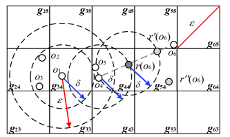
Figure 3. $o_{i}\,(1\leq i\leq 6)$ at $\textit{dt}_{2}$ in Figure 1 ($\rho=3$)

Example 3.

In Figure 2b, there are two minimal groups, i.e., $\mathcal{M}_{1}({o_{1}})$
$=\{o_{1},o_{2},o_{3}\}$ and $\mathcal{M}_{1}({o_{4}})=\{o_{4},o_{5},o_{6}\}$. In Figure 3, there is only one minimal group before smoothing, i.e., $\mathcal{M}_{2}({o_{1}})=\{o_{1},o_{2},o_{3}\}$. Further, given the current $k=2$, both $s$ and $\tilde{s}$ of $o_{2}$ is $o_{1}$ and $\tilde{s}.\tilde{l}=o_{1}.l_{1}$.

We propose to use the location of a seed point $s$ to smooth the location of a non-seed point $o\,(o\in\mathcal{M}_{k-1}(\tilde{s}))$ at $\textit{dt}_{k}$. In order to guarantee the effectiveness of smoothing, Definition 12 gives two constraints when generating minimal groups: (i) $d(o,s)<\delta\,(\delta\leq\varepsilon)$ and (ii) $\lvert\mathcal{M}_{k}(s)\rvert\geq\rho$. Setting $\delta$ to a small value, the first constraint ensures that $o\in\mathcal{M}_{k}(s)$ are close neighbors at $\textit{dt}_{k}$. Specifically, we require $\delta\leq\varepsilon$ because this makes it very likely that trajectories in the same minimal group are in the same cluster. The second constraint avoids small neighbor sets $\mathcal{N}_{\delta}(s)$. Specifically, using an ”uncertain border” point as a ”pivot” to smooth the movement of other trajectories may lead to an abrupt change between clusterings or a low-quality clustering (according to the quality metrics of traditional clustering). We present the algorithm for generating minimal groups in Section 5.2.

Based on the above analysis, we formalize the historical cost of $o$ w.r.t. its adjustment $r(o)$ at $\textit{dt}_{k}$, denoted as $\mathcal{TC}_{k}(r(o))$, as follows.

(3) $$\mathcal{TC}_{k}(r(o))=\left(\lceil\frac{d(r(o),\tilde{s}.l)}{\delta}\rceil-1\right)^{2}$$

$$s.t.\,d(r(o),o.\tilde{l})\leq\mu\cdot(o.t-o.\tilde{t}),$$

where $o\in\mathcal{M}_{k-1}(\tilde{s})\backslash\{\tilde{s}\}$. Given the threshold $\delta$, the larger the distance between $r(o)$ and $\tilde{s}.l$, the higher the historical cost. Here, we use the degree of closeness (i.e., $\lceil\frac{d(r(o),\tilde{s}.l)}{\delta}\rceil-1$) instead of $d(r(o),\tilde{s}.l)$ to evaluate the historical cost, due to two reasons. First, constraining the exact relative distance between any two trajectories during a time interval may be too restrictive, as it varies over time in most cases. Second, using the degree of closeness to constrain the historical cost is sufficient to obtain a smooth evolution of clusterings.

Total cost $\bm{\mathcal{F}_{k}}$

Formulas 2 and 3 give the snapshot cost and historical cost for each trajectory $o$ w.r.t. its adjustment $r(o)$, respectively. However, the first measures the distance while the latter evaluates the degree of proximity. Thus, we normalize them to a specific range $[0,1)$:

(4) $$\mathcal{SC}_{k}(r(o))=\left(\frac{d(r(o),o.l)}{4\mu\cdot\Delta t+\delta}\right)^{2}s.t.\,d(r(o),o.\tilde{l})\leq\mu\cdot(o.t-o.\tilde{t})$$

(5) $$\mathcal{TC}_{k}(r(o))=\left(\frac{\lceil\frac{d(r(o),\tilde{s}.l)}{\delta}\rceil-1}{\frac{4\mu\cdot\Delta t+\delta}{\delta}}\right)^{2}$$

$$s.t.\,d(r(o),o.\tilde{l})\leq\mu\cdot(o.t-o.\tilde{t}),$$

where $o\in\mathcal{M}_{k-1}(\tilde{s})\backslash\{\tilde{s}\}$ and $\Delta t$ is the duration of a time step. Clearly, $\mathcal{SC}_{k}(r(o))\geq 0$ and $\mathcal{TC}_{k}(r(o))\geq 0$. Thus, we only need to prove $\mathcal{SC}_{k}(r(o))<1$ and $\mathcal{TC}_{k}(r(o))<1$.

Lemma 1.

If $d(o.l,o.\tilde{l})\leq(o.t-o.\tilde{t})\cdot\mu$ then ${d(r(o),o.l)}\leq 4\mu\cdot\Delta t$.

Proof.

According to our strategy of mapping original timestamps (Section 2.1), $o.t-o.\tilde{t}\leq 2\Delta t$. Considering the speed constraint of the road network, $d(r(o),o.\tilde{l})\leq\mu\cdot(o.t-o.\tilde{t})$. Further, $d(r(o),o.l)\leq d(o.l,o.\tilde{l})+d(r(o),o.\tilde{l})$ due to the triangle inequality. Thus, we get $d(r(o),o.l)\leq d(o.l,o.\tilde{l})+2\mu\cdot\Delta t$. Since $d(o.l,o.\tilde{l})\leq(o.t-o.\tilde{t})\cdot\mu$, ${d(r(o),o.l)}\leq 4\mu\cdot\Delta t$. ∎

It follows from Lemma 1 that $\mathcal{SC}_{k}(r(o))<1$ if $d(o.l,o.\tilde{l})\leq(o.t-o.\tilde{t})\cdot\mu$. However, $d(o.l,o.\tilde{l})\leq(o.t-o.\tilde{t})\cdot\mu$ does not necessarily hold. To address this problem, we pre-process $o.l$ according to $o.\tilde{l}$ so that it follows the speed constraint before conducting evolutionary clustering. The details are given in Section 4.3.

Lemma 2.

If $d(\tilde{s}.l,\tilde{s}.\tilde{l})\leq(\tilde{s}.t-\tilde{s}.\tilde{t})\cdot\mu$ then $d(r(o),\tilde{s}.l)\leq 4\mu\cdot\Delta t+\delta$.

Proof.

We have $d(r(o),o.\tilde{l})\leq 2\mu\cdot\Delta t$ according to Lemma 1. Further, $d(o.\tilde{l},\tilde{s}.\tilde{l})\leq\delta$ according to Definition 12. Since $d(r(o),\tilde{s}.l)\leq d(r(o),o.\tilde{l})+d(o.\tilde{l},\tilde{s}.l)\leq d(r(o),o.\tilde{l})+d(o.\tilde{l},\tilde{s}.\tilde{l})+d(\tilde{s}.\tilde{l},\tilde{s}.l)$, we get $d(r(o),\tilde{s}.l)\leq 4\mu\cdot\Delta t+\delta$. ∎

According to Lemma 2, we can derive $\lceil\frac{4\mu\cdot\Delta t+\delta}{\delta}\rceil-1<\frac{4\mu\cdot\Delta t+\delta}{\delta}$ and thus $\mathcal{TC}_{k}(r(o))<1$. Letting $4\mu\cdot\Delta t+\delta=\pi$, the total cost $\mathcal{F}_{k}$ is:

(6) $$\mathcal{F}_{k}= \sum_{o,\tilde{s}\in\Theta_{k}\wedge o\neq\tilde{s}}\frac{1}{\pi^{2}}\left(d(r(o),o.l)^{2}+\alpha\cdot\left(\delta\cdot\left(\lceil\frac{d(r(o),\tilde{s}.l)}{\delta}\rceil-1\right)\right)^{2}\right)$$

$$s.t.\,\forall o\in\Theta_{k}\,(d(r(o),o.\tilde{l})\leq\mu\cdot(o.t-o.\tilde{t})),$$

where ${\Theta}_{k}=\mathcal{O}_{k}\cap(\bigcup_{\tilde{s}\in\mathcal{S}_{k-1}}\mathcal{M}_{k-1}(\tilde{s}))$. Formula 6 indicates that we do not smooth the location of $o$ at $\textit{dt}_{k}$ if $o$ is not summarized in any minimal group at $\textit{dt}_{k-1}$. This is in accordance with the basic idea that we conduct smoothing by exploring the neighboring trajectories. We can now formulate our problem.

Definition 13.

Given a snapshot $\mathcal{O}_{k}$, a set of previous minimal groups $\bigcup_{\tilde{s}\in\mathcal{S}_{k-1}}\mathcal{M}_{k-1}(\tilde{s})$, a time duration $\Delta t$, a speed constraint $\mu$, and parameters $\alpha$, $\delta$, $\varepsilon$, minPts and $\rho$, evolutionary clustering of streaming trajectories (ECO) is to

• find a set of adjustments $\mathcal{R}_{{k}_{opt}}$, such that $\mathcal{R}_{k_{opt}}=\arg\min_{\mathcal{R}_{k}}\mathcal{F}_{k}$;

• compute a set of clusters $\mathcal{C}_{k}$ over $\mathcal{R}_{k_{opt}}$.

Specifically, each adjustment of $o.l\in\mathcal{R}_{k_{opt}}$ is denoted as $r_{opt}(o)$ and is then used as the previous location of $o$ (i.e. $o.\tilde{l}$) at $\textit{dt}_{k+1}$ for evolutionary clustering.

Example 4.

Following Example 3, ECO first finds a set of adjustments $\mathcal{R}_{{2}_{opt}}=\{r_{opt}(o_{i})|1\leq i\leq 12\}$ at $\textit{dt}_{2}$. Then, it performs clustering over $\mathcal{R}_{{2}_{opt}}$ and gets $\mathcal{C}_{2}=\{c_{1},c_{2}\}$, where $c_{1}=\{o_{i}|1\leq i\leq 6\}$ and $c_{2}=\{o_{i}|7\leq i\leq 12\}$. Note that we only show $r_{opt}(o_{6})(\,=r(o_{6}))$ and $r_{opt}(o_{10})(\,=r(o_{10}))$ in Figures 1 and 3 because $r_{opt}(o_{i})=o_{i}.l\,(1\leq i\leq 12\wedge i\neq 6\wedge i\neq 10)$ at $\textit{dt}_{2}$.

Clearly, the objective function in Formula 6 is neither continuous nor differentiable. Thus, computing the optimal adjustments using existing solvers involves iterative processes (Song et al., 2015) that are too expensive for online scenarios. We thus prove that Formula 6 can be solved approximately in linear time in Section 4.

4. Computation of Adjustments

Given the current time step $\textit{dt}_{k}$, we start by decomposing $\mathcal{F}_{k}$ at the unit of minimal groups as follows,

(7) $$\mathcal{F}_{k} =\sum_{\tilde{s}\in\mathcal{S}_{k-1}}f_{k}(\tilde{s}.l)$$

$$=\sum_{\tilde{s}\in\mathcal{S}_{k-1}}\sum_{o\in\Omega}\left(d(r(o),o.l)^{2}+\alpha\cdot\left(\delta\cdot\left(\lceil\frac{d(r(o),\tilde{s}.l)}{\delta}\rceil-1\right)\right)^{2}\right)$$

$$s.t.\,\forall o\in\Theta_{k}\,(d(r(o),o.\tilde{l})\leq\mu\cdot(o.t-o.\tilde{t})),$$

where $\Theta_{k}=\mathcal{O}_{k}\cap(\bigcup_{\tilde{s}\in\mathcal{S}_{k-1}}\mathcal{M}_{k-1}(\tilde{s}))$, $\Omega=\mathcal{M}_{k-1}(\tilde{s})\backslash\{\tilde{s}\}$, $r(o)$ is the adjustment of $o.l$ at $\textit{dt}_{k}$, $\tilde{s}$ is the seed point of $o$ at $\textit{dt}_{k-1}$, and $\tilde{s}.l$ is the location of $\tilde{s}$ at $\textit{dt}_{k}$. We omit the multiplier $\frac{1}{\pi^{2}}$ from Formula 6 because $\Delta t$, $\mu$, and $\delta$ are constants and do not affect the results.

4.1. Linear Time Solution

We show that Formula 7 can be solved approximately in linear time. However, Formula 7 uses each previous seed point $\tilde{s}$ for smoothing, and such points may also exhibit unusual behaviors from $\textit{dt}_{k-1}$ to $\textit{dt}_{k}$. Moreover, $\tilde{s}$ may not be in $\mathcal{O}_{k}$. We address these problems in Section 4.2 by proposing a seed point shifting strategy, and we assume here that $\tilde{s}\in\mathcal{O}_{k}$ has already been smoothed, i.e., $r(\tilde{s})=\tilde{s}.l$.

Lemma 3.

$\mathcal{F}_{k}$ achieves the minimum value if each $f_{k}(\tilde{s}.l)\,(\tilde{s}\in\mathcal{S}_{k-1})$ achieves the minimum value.

Proof.

To prove this, we only need to prove that $f_{k}(\tilde{s}.l)$ and ${f}_{k}(\tilde{s}^{\prime}.\tilde{l})$ $(\tilde{s}\neq\tilde{s}^{\prime}\wedge\tilde{s},\tilde{s}^{\prime}\in\mathcal{S}_{k-1})$ do not affect each other. This can be established easily, as we require $\mathcal{M}_{k-1}(\tilde{s})\cap\mathcal{M}_{k-1}(\tilde{s}^{\prime})=\emptyset$. We thus omit the details due to space limitation. ∎

Lemma 3 implies that Formula 7 can be solved by minimizing each $f_{k}(\tilde{s}.l)$ ($\tilde{s}\in\mathcal{S}_{k-1}$). Next, we further ”push down” the cost shown in Formula 7 to each pair of $o\,(o\in\mathcal{M}_{k-1}(\tilde{s})\backslash\{\tilde{s}\})$ and $\tilde{s}$.

$$f_{k}(r(o),\tilde{s}.l) = \left(d(r(o),o.l)^{2}+\alpha\cdot\left(\delta\cdot\left(\lceil\frac{d(r(o),\tilde{s}.l)}{\delta}\rceil-1\right)\right)^{2}\right)$$

(8) $$s.t. \,d(r(o),o.\tilde{l})\leq\mu\cdot(o.t-o.\tilde{t})$$

Lemma 4.

$f_{k}(\tilde{s}.l)$ achieves the minimum value if each $f_{k}(r(o),\tilde{s}.l)\,$
$(o\in\mathcal{M}_{k-1}(\tilde{s})\cap\mathcal{O}_{k}\backslash\{\tilde{s}\})$ achieves the minimum value.

Proof.

The proof is straightforward, because $f_{k}(r(o),\tilde{s}.l)$ and $f_{k}(r^{\prime}(o),\tilde{s}.l)$ $(o,o^{\prime}\in\mathcal{M}_{k-1}(\tilde{s})\cap\mathcal{O}_{k}\backslash\{\tilde{s}\}\wedge o\neq o^{\prime})$ are independent of each other. ∎

According to Lemma 4, the problem is simplified to computing $r_{opt}(o)=\arg\min_{r(o)}f_{k}(r(o),\tilde{s}.l)$ ($o\in\mathcal{M}_{k-1}(\tilde{s})\cap\mathcal{O}_{k}\backslash\{\tilde{s}\}$) given $\tilde{s}$. However, Formula 4.1 is still intractable as its objective function is not continuous. We thus aim to transform it into a continuous function. Before doing so, we cover the case where the computation of $r_{opt}(o)$ w.r.t a trajectory $o$ can be skipped.

Lemma 5.

If $d(o.l,\tilde{s}.l)\leq\delta$ then $o.l=\arg\min_{r(o)}f_{k}(r(o),\tilde{s}.l)$.

Proof.

Let $r(o)\,(r(o)\neq o.l)$ be an adjustment of $o.l$. Given $d(o.l,\tilde{s}.l)\leq\delta$, $\mathcal{TC}_{k}(o.l)=0\leq\mathcal{TC}_{k}(r(o))$. On the other hand, as $d(r(o),o.l)>d(o.l,o.l)=0$, the snapshot cost $\mathcal{SC}_{k}(o.l)=0<\mathcal{SC}_{k}(r(o))$. Thus, $r_{opt}(o)=o.l$ if $d(o.l,\tilde{s}.l)\leq\delta$. ∎

A previous study (Kim and Han, 2009) smooths the distance between each pair of neighboring nodes no matter their relative distances. In contrast, Lemma 5 suggests that if a non-seed point remains close to its previous seed point at the current time step, smoothing can be ignored. This avoids over-smoothing close trajectories. Following Example 4, $o_{2}.l=\arg\min_{r(o_{2})}f_{2}(r(o_{2}),o_{1}.l)$.

Definition 14.

A circle is given by $\mathcal{Q}(e,x)$, where $e$ is the center and $x$ is the radius.

Definition 15.

A segment connecting two locations $l$ and $l^{\prime}$ is denoted as $\textit{se}(l,l^{\prime})$. The intersection of a circle $\mathcal{Q}(e,x)$ and a segment $\textit{se}(l,l^{\prime})$ is denoted as $\textit{se}(l,l^{\prime})\oplus\mathcal{Q}(e,r)$.

Figure 3 shows a circle $\mathcal{Q}(o_{1}.l,\delta)$ that contains $o_{1}.l$, $o_{2}.l$, and $o_{3}.l$. Further, $r(o_{6})=\textit{se}(o_{6}.l,o_{4}.l)\oplus\mathcal{Q}(o_{4}.l,\delta)$.

Lemma 6.

$\textit{se}(o.l,\tilde{s}.l)\cap\mathcal{Q}(o.\tilde{l},\mu\cdot(o.t-o.\tilde{t}))\neq\emptyset$.

Proof.

In Section 3.2, we constrain $o.t-o.\tilde{t}\leq\mu\cdot\Delta t$ before smoothing, which implies that $o.l\in\mathcal{Q}(o.\tilde{l},\mu\cdot(o.t-o.\tilde{t}))$. Hence, $\textit{se}(o.l,\tilde{s}.l)\cap\mathcal{Q}(o.\tilde{l},\mu\cdot(o.t-o.\tilde{t}))\neq\emptyset$. ∎

In Figure 4, given $o_{6}.t-o_{6}.\tilde{t}=3$, $o_{6}.l\in\textit{se}(o_{6}.l,o_{4}.l)\cap\mathcal{Q}(o_{6}.\tilde{l},3\mu)$.

Omitting the speed constraint

We first show that without utilizing the speed constraint, an optimal adjustment $r_{opt^{\prime}}(o)$ of $o.l$ that minimizes $f(r(o),\tilde{s}.l)$ can be derived in constant time. Based on this, we explain how to compute $r_{opt}$ based on $r_{opt^{\prime}}(o)$.

Lemma 7.

$\forall r^{\prime}(o)\notin\textit{se}(o.l,\tilde{s}.l)(\exists r(o)\in\textit{se}(o.l,\tilde{s}.l)(f_{k}(r(o),\tilde{s}.l)\leq f_{k}(r^{\prime}(o),\tilde{s}.l)))$.

Proof.

Let $d(o.l,\tilde{s}.l)=y$. First, we prove that $\forall r^{\prime}(o)\notin\mathcal{Q}(\tilde{s}.l,y)$
$(\exists r(o)\in\textit{se}(o.l,\tilde{s}.l)(f_{k}(r^{\prime}(o),\tilde{s}.l)\geq f_{k}(r(o),\tilde{s}.l)))$. Two cases are considered, i.e., (i) $d(r^{\prime}(o),o.l)\leq y$ and (ii) $d(r^{\prime}(o),o.l)>y$. For the first case, we can always find an adjustment $r(o)\in\textit{se}(o.l,\tilde{s}.l)$, such that $d(r^{\prime}(o),o.l)=d(r(o),o.l)$. Hence, $\mathcal{SC}_{k}(r^{\prime}(o))=\mathcal{SC}_{k}(r(o))$. However, we have $\mathcal{TC}_{k}(r^{\prime}(o))\geq\mathcal{TC}_{k}(r(o))$ due to $d(r^{\prime}(o),\tilde{s}.l)>d(r(o),\tilde{s}.l)$. Thus, $f_{k}(r^{\prime}(o),\tilde{s}.l)\geq f_{k}(r(o),\tilde{s}.l)$. For the second case, it is clear that $\forall r(o)\in\textit{se}(o.l,\tilde{s}.l)(\mathcal{SC}_{k}(r^{\prime}(o))>\mathcal{SC}_{k}(r(o))\wedge\mathcal{TC}_{k}(r^{\prime}(o))\geq\mathcal{TC}_{k}(r(o)))$. Thus, $f_{k}(r^{\prime}(o),\tilde{s}.l)>f_{k}(r(o),\tilde{s}.l)$.

Second, we prove that $\forall r^{\prime}(o)\in\mathcal{Q}(\tilde{s}.l,y)\backslash\textit{se}(o.l,\tilde{s}.l)(\exists r(o)\in\textit{se}(o.l,\tilde{s}.l)(f_{k}(r^{\prime}(o),\tilde{s}.l)\geq f_{k}(r(o),\tilde{s}.l)))$. We can always find $r(o)\in\textit{se}(o.l,\tilde{s}.l)$, such that $d(r^{\prime}(o),\tilde{s}.l)=d(r(o),\tilde{s}.l)$. Hence, $\mathcal{TC}_{k}(r^{\prime\prime}(o))$
$=\mathcal{TC}_{k}(r(o))$. However, in this case $\mathcal{SC}_{k}(r^{\prime}(o))$ $>\mathcal{SC}_{k}(r(o))$ due to $r(o)\in\textit{se}(o.l,\tilde{s}.l)\wedge r^{\prime}(o)\notin\textit{se}(o.l,\tilde{s}.l)$. Thus, we have $f_{k}(r^{\prime}(o),\tilde{s}.l)$
$>f_{k}(r(o),\tilde{s}.l)$. ∎

In Figure 3, $f(r(o_{6}),o_{4}.l)\leq f(r^{\prime\prime}(o_{6}),o_{4}.l)$ and $f(r^{\prime}(o_{6}),o_{4}.l)\leq f(r^{\prime\prime}(o_{6}),o_{4}.l)$ due to $r^{\prime\prime}(o_{6})\notin\textit{se}(o_{4}.l,o_{6}.l)$. Lemma 7 indicates that if we ignore the speed constraint in Formula 4.1, we can search $r_{opt^{\prime}}(o)$ just on $\textit{se}(o.l,\tilde{s}.l)$ without missing any result.

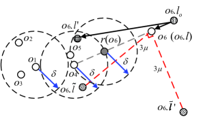
Figure 4. An example of speed-based pre-processing, i.e., $\bm{o_{6}.l_{o}\rightarrow o_{6}}$, in Figure 3 ($\bm{\rho=3}$)

Lemma 8.

Let $d(r_{opt^{\prime}}(o),\tilde{s}.l)=b_{opt^{\prime}}\cdot\delta$. If $d(o.l,\tilde{s}.l)>\delta$ then $b_{opt^{\prime}}\in\left\{{\bm{\mathrm{N}}^{*}}\cap[\lambda_{1},\lambda_{2}]\right\}\cup\lambda_{2}$, where $\lambda_{1}=\frac{d(\tilde{s}.l,o.\tilde{l})-\mu\cdot(o.t-{o}.\tilde{t})}{\delta}$, $\lambda_{2}=\frac{d(o.l,\tilde{s}.l)}{\delta}$ and ${\bm{\mathrm{N}}}^{*}$ is the natural numbers.

Proof.

We start by proving $\max\{\lambda_{1},1\}\leq b_{opt^{\prime}}\leq\lambda_{2}$. First, we have $r_{opt^{\prime}}(o)\in\textit{se}(o.l,\tilde{s}.l)$ according to Lemma 7. Thus, $b_{opt^{\prime}}\cdot\delta\leq d(o.l,\tilde{s}.l)$, i.e., $b_{opt^{\prime}}\leq\lambda_{2}$. Further, $\forall r(o)\in\textit{se}(o.l,\tilde{s}.l)(d(r(o),\tilde{s}.l)+d(r(o),o.\tilde{l})\geq d(\tilde{s}.l,o.\tilde{l}))$ due to the triangle inequality. Thus, $b_{opt^{\prime}}\cdot\delta+\mu\cdot(o.t-{o}.\tilde{t})\geq d(\tilde{s}.l,o.\tilde{l})$, i.e., $b_{opt^{\prime}}\geq\lambda_{1}$. Moreover, $\forall r^{\prime}(o)\in\textit{se}(o.l,\tilde{s}.l)((0<d(r^{\prime}(o),\tilde{s}.l)<\delta\wedge d(r(o),\tilde{s}.l)=\delta)\Rightarrow(\mathcal{TC}(r^{\prime}(o))=\mathcal{TC}(r(o))\wedge\mathcal{SC}(r^{\prime}(o))>\mathcal{SC}(r(o))))$. Thus, we get $b_{opt^{\prime}}\geq 1$.

Next, we prove $\forall r^{\prime}(o),r(o)\in\textit{se}(o.l,\tilde{s}.l)((b-1)\cdot\delta<d(r^{\prime}(o),\tilde{s}.l)$
$<b\cdot\delta\wedge d(r(o),\tilde{s}.l)=b\cdot\delta\wedge 1\leq b\leq\lfloor\lambda_{2}\rfloor\wedge b\in\bm{\mathrm{N}}^{*})\Rightarrow(f(r(o),\tilde{s}.l)<f(r^{\prime}(o),\tilde{s}.l)))$. According to Formula 5, $\mathcal{TC}(r(o))=\mathcal{TC}(r^{\prime}(o))$. Further, $d(o.l,r^{\prime}(o))=d(o.l,\tilde{s}.l)-d(r^{\prime}(o),\tilde{s}.l)$ and $d(o.l,r(o))=d(o.l,\tilde{s}.l)$ $-b\cdot\delta$. As $d(r^{\prime}(o),\tilde{s}.l)<b\cdot\delta$ we have $\mathcal{SC}(r(o))<\mathcal{SC}(r^{\prime}(o))$. Thus, $b_{opt^{\prime}}\notin[1,\lfloor\lambda_{2}\rfloor]\backslash\bm{\mathrm{N}}^{*}$.

Finally, we prove $\forall r^{\prime}(o)\in\textit{se}(o.l,\tilde{s}.l)(b\cdot\delta\leq d(r^{\prime}(o),\tilde{s}.l)\wedge\lfloor\lambda_{2}\rfloor<b\leq\lambda_{2})\Rightarrow(f(o.l,\tilde{s}.l)<f(r^{\prime}(o),\tilde{s}.l)))$. Similar to the above proof, in this case $\mathcal{TC}(r^{\prime}(o))=\mathcal{TC}(o.l)\wedge\mathcal{SC}(r^{\prime}(o))>\mathcal{SC}(o.l)$. Thus, $b_{opt^{\prime}}\notin(\lfloor\lambda_{2}\rfloor,\lambda_{2}]\backslash\{\lambda_{2}\}$. ∎

In Figure 3, we have $r_{opt^{\prime}}(o_{6})\in\{o_{6}.l,r(o_{6}),r^{\prime}(o_{6})\}$. Based on Lemmas 5 to 8, we let $d(r(o),\tilde{s}.l)=b\cdot\delta$ and simplify Formula 4.1 to the following function:

(9) $$\quad f_{k}(b,\tilde{s}.l) =\left(d(o.l,\tilde{s}.l)-b\cdot\delta\right)^{2}+\alpha\cdot\left(\delta\cdot\left(b-1\right)\right)^{2}$$

$$s.t.\,\,b\in\left\{{\bm{\mathrm{N}}^{*}}\cap[\lambda_{1},\lambda_{2}]\right\}\cup\lambda_{2},$$

where $\lambda_{1}=\frac{d(\tilde{s}.l,o.\tilde{l})-\mu\cdot(o.t-o.\tilde{t})}{\delta}$ and $\lambda_{2}=\frac{d(o.l,\tilde{s}.l)}{\delta}$. The snapshot cost $\left(d(o.l,\tilde{s}.l)-b\cdot\delta\right)^{2}$ is derived according to Lemma 7, i.e., $o.l,r_{opt^{\prime}}(o)$ and $\tilde{s}.l$ are on the same line segment; while the historical cost $\left(\delta\cdot\left(b-1\right)\right)^{2}$ is obtained by simply plugging $d(r(o),\tilde{s}.l)=b\cdot\delta$ into Formula 4.1. The objective function in Formula 9 is a continuous. Thus, the $b_{opt^{\prime}}\,(\in\left\{{\bm{\mathrm{N}}^{*}}\cap[\lambda_{1},\lambda_{2}]\right\}\cup\lambda_{2})$ that minimizes the function can be obtained in constant time without sacrificing accuracy.

Example 5.

Continuing Example 4 and given $d(o_{6}.l,o_{4}.l)=25$, $\alpha=2.1$ and $\delta=10$, we get $b_{opt^{\prime}}=1$ and $r_{opt^{\prime}}(o_{6})=r(o_{6})$.

Introducing the speed constraint

Recall that $r_{opt^{\prime}}(o)$ is the optimal adjustment of $o.l$ without taking the speed constraint in Formula 4.1 into account, while $r_{opt}(o)$ takes the constraint into account. We have narrowed the range of $r_{opt^{\prime}}$ to a set of discrete locations on $\textit{se}(o.l,\tilde{s}.l)$ without sacrificing any accuracy. Further, if $r_{opt^{\prime}}\in\mathcal{Q}(o.\tilde{l},\mu\cdot\Delta t)$ then $r_{opt}(o)=r_{opt^{\prime}}(o)$. However, if $r_{opt^{\prime}}\notin\mathcal{Q}(o.\tilde{l},\mu\cdot\Delta t)$, $r_{opt^{\prime}}(o)$ is an invalid adjustment. In this case, letting $d(r_{opt}(o),\tilde{s}.l)=b_{opt}\cdot\delta$, we propose to approximate $r_{opt}$ by searching only in the narrowed range of $r_{opt^{\prime}}$, i.e., we propose to compute $b_{opt}$ approximately as follows.

(10) $$b_{opt}=\arg\min_{b\in\left\{{\rm{N}^{*}}\cap[\lambda_{1},\lambda_{2}]\right\}\cup\lambda_{2}}\lvert b-b_{opt^{\prime}}\rvert$$

$$s.t.\,\,\mathcal{Q}(o.\tilde{l},\mu\cdot(o.t-o.\tilde{t}))\cap\mathcal{Q}(\tilde{s}.l,b\cdot\delta)\neq\emptyset,$$

where $\mathcal{Q}(o.\tilde{l},\mu\cdot(o.t-o.\tilde{t}))\cap\mathcal{Q}(\tilde{s}.l,b\cdot\delta)\neq\emptyset$ indicates that $r_{opt}(o)\in\mathcal{Q}(o.\tilde{l},\mu\cdot(o.t-o.\tilde{t}))$ must hold due to $d(r_{opt}(o),\tilde{s}.l)=b_{opt}\cdot\delta$. After getting $b_{opt^{\prime}}$, $b_{opt}$ can be located according to $\textit{se}(o.l,\tilde{s}.l)\oplus\mathcal{Q}(o.\tilde{l},\mu\cdot(o.t-o.\tilde{t}))$ in constant time. Following Example 5 and given $o_{6}.t-o_{6}.\tilde{t}=3$ and $\mu=9$, $r_{opt}(o_{6})=r(o_{6})$ if $o_{6}.l_{1}=o_{6}.\tilde{l}$, while $r_{opt}(o_{6})=o_{6}.l$ if $o_{6}.l_{1}=o_{6}.\tilde{l}^{\prime}$ (shown in Figure 4). Specifically, in the latter case, $o_{6}.l$ is the only feasible solution of $r_{opt}(o_{6})$ according to Formula 10, as $\textit{se}(o_{6}.l,o_{4}.l)\oplus\mathcal{Q}(o_{6}.\tilde{l}^{\prime},3\mu)=o_{6}.l$. Note that computing $r_{opt}$ using Formula 10 may not yield an optimal value that minimizes $f_{k}(r(o),\tilde{s}.l)$. This is because we approximate the feasible region of $r_{opt}$ by the narrowed range of $r_{opt^{\prime}}$ and may miss an $r(o)\,(r(o)\in\mathcal{Q}(o.\tilde{l},\mu\cdot(o.t-o.\tilde{t}))\backslash\textit{se}(o.l,\tilde{s}.l))$ that minimizes Formula 4.1. However, experiments show that $r_{opt^{\prime}}=r_{opt}$ in most case. The underlying reasons are that the maximum distance a trajectory can move under the speed limitation is generally far larger than the distance a trajectory actually moves between any two time steps and that we constrain $d(o.l,o.\tilde{l})\leq\mu\cdot(o.t-o.\tilde{t})$ before smoothing, which ”repairs” large noise to some extent. So far, the efficiency of computing $r_{opt}(o)$ using Formula 4.1 has been improved to $O(1)$ time complexity.

4.2. Shifting of Seed Points

Section 4.1 assumes that the previous seed point $\tilde{s}.l$ evolves gradually when smoothing $o\in\mathcal{M}_{k-1}(\tilde{s})\cap\mathcal{O}_{k}\backslash\{\tilde{s}\}$ at $\textit{dt}_{k}$, which is not always true. Thus, $\tilde{s}.l$ may also need to be smoothed. We first select a ”pivot” for smoothing $\tilde{s}.l$. An existing method (Song et al., 2015) maps the noise point to the accurate point that is closest to it in a batch mode. Inspired by this, we smooth $\tilde{s}.l$ using $o.l$ ($o\in\mathcal{M}_{k-1}(\tilde{s})\cap\mathcal{O}_{k}$), which is a set of discrete locations. This is based on the observation that the travel companions of each trajectory evolves gradually due to the smooth movement of trajectories. Next, we determine which trajectory $o$ should be selected as a ”pivot” to smooth $\tilde{s}.l$.

Evolutionary clustering assigns a low cost (cf. Formula 1) if the clusterings change smoothly during a short time period. Since we use cost embedding, we consider the location of a trajectory $o$ as evolving smoothly if the distance between $o$ and $o^{\prime}$ ($o^{\prime}\in\mathcal{M}_{k-1}(\tilde{s})\cap\mathcal{O}_{k}\backslash\{o\}$) varies only little between two adjacent time steps. This is essentially evaluated by $f_{k}(o)$ (cf. Formula 7), which measures the cost of smoothing $o^{\prime}$ ($o^{\prime}\in\mathcal{M}_{k-1}(\tilde{s})\cap\mathcal{O}_{k}\backslash\{o\}$) according to $o$. Hence, we select the ”pivot” for smoothing $\tilde{s}.l$ using the following formula:

(11) $$\tilde{s}_{\mathit{new}}=\arg\min_{o\in\mathcal{M}_{k-1}(\tilde{s})\cap\mathcal{O}_{k}}f_{k}(o)$$

After obtaining a ”pivot” $\tilde{s}_{\mathit{new}}$, instead of first smoothing $\tilde{s}.l$ according to $\tilde{s}_{\mathit{new}}.l$ and then smoothing $o.l(o\in\mathcal{M}_{k-1}(\tilde{s})\backslash\{\tilde{s}\})$ by $\tilde{s}.l$, we shift the seed point of $o\in\mathcal{M}_{k-1}(\tilde{s})\backslash\{\tilde{s}\}$ from $\tilde{s}$ to $\tilde{s}_{\mathit{new}}$ and use $\tilde{s}_{\mathit{new}}$ to smooth other trajectories $o\,(o\neq\tilde{s}_{\mathit{new}})$. The reasons are: (i) by Formula 11, $\tilde{s}_{\mathit{new}}$ is the trajectory with the smoothest movement from $\textit{dt}_{k-1}$ to $\textit{dt}_{k}$ among trajectories in $\mathcal{M}_{k-1}(\tilde{s})$, and thus it is less important to smooth it; (ii) we can save $\lvert\mathcal{M}_{k-1}(\tilde{s})\rvert-1$ computations in Formula 7. Formula 11 suggests that the seed point may not be shifted, i.e., $\tilde{s}_{\mathit{new}}$ may be $\tilde{s}$. Intuitively, when computing $\tilde{s}_{\mathit{new}}$, the locations of all trajectories in their corresponding minimal group are smoothed; and with the seed point shifting strategy, smoothing does not require that the previous seed point is active at the current time step.

Example 6.

Continuing Example 5, given $f_{2}(o_{6}.l)=\min\{f_{2}(o_{4}.l),$
$f_{2}(o_{5}.l),f_{2}(o_{6}.l)\}$, $\tilde{s}_{\mathit{new}}=\tilde{s}=o_{6}$. When calculating $\tilde{s}_{\mathit{new}}$, we get $r_{opt}(o_{4})=o_{4}.l$, $r_{opt}(o_{5})=o_{5}.l$, and $r_{opt}(o_{6})=r(o_{6})$.

The time complexity of smoothing a minimal group $\mathcal{M}_{k-1}(\tilde{s})$ is $O(\lvert\mathcal{M}_{k-1}(\tilde{s})\rvert^{2})$.

4.3. Speed-based Pre-processing

We present the pre-processing that forces each to-be-smoothed trajectory $o\in\mathcal{O}_{k}\cap(\bigcup_{\tilde{s}\in\mathcal{S}_{k-1}}\mathcal{M}_{k-1}(\tilde{s}))$ to observe the speed constraint. The pre-processing guarantees the correctness of the normalization of the snapshot and historical costs and can repairs large noise to some extent. We denote the location of $o$ before pre-processing as $o.l_{o}$ and the possible location after as $o.l_{p}$.

A naive pre-processing strategy is to map $o.l_{o}$ to a random location on or inside $\mathcal{Q}(o.\tilde{l},\mu\cdot\Delta t)$. However, this random strategy may make the smoothing less reasonable.

Example 7.

Continuing Example 5, Figure 4 shows two possible locations $o_{6}.l$ and $o_{6}.l^{\prime}$ of $o_{6}.l_{o}$, both of which are chosen at random while observing the speed constraint, i.e., they are located on and inside $\mathcal{Q}(o_{6}.\tilde{l},3\mu)$, respectively. Since $d(o_{6}.l^{\prime},o_{4}.l)<\delta<d(o_{6}.l,o_{4}.l)$, the adjustment of $o_{6}.l^{\prime}$ is $o_{6}.l^{\prime}$ itself while that of $o_{6}.l$ is $r(o_{6})$.

In this example, $o_{6}.l^{\prime}$ is less reasonable than $r(o_{6})$. Specifically, according to the minimum change principle (Song et al., 2015), the changes to the data distribution made by the speed-based pre-processing and the neighbor-based smoothing should be as small as possible. However, considering $d(o_{6}.l_{o},o_{4}.l)$, $o_{6}.l^{\prime}$ is too close to $o_{4}.l$ compared with $o_{6}.l$ and $r(o_{6})$. Given a pre-processed location $o.l$, its change due to smoothing has already been minimized through Formula 4.1. Thus, to satisfy the minimum change principle, we just need to make the impact of speed-based pre-processing on neighbor-based smoothing as small as possible. Hence, we find the pre-processed $o.l$ via the speed constraint as follows.

(12) $$o.l=\arg\min_{o.l_{p}}\left\lvert d(o.l_{p},\tilde{s}.l)-d(o.l_{o},\tilde{s}.l)\right\rvert$$

$$s.t.\,d(o.l_{p}-o.\tilde{l})\leq\mu\cdot(o.t-o.\tilde{t})$$

This suggests that the difference between $d(o.l,\tilde{s}.l)$ and $d(o.l_{o},\tilde{s}.l))$ is expected to be as small as possible, in order to mitigate the effect of speed-based pre-processing on computing historical cost. Before applying Formula 12, we pre-process $\tilde{s}.l$ so that it also follows the speed constraint:

(13) $$\tilde{s}.l=\arg\min_{\tilde{s}.l_{p}}d(\tilde{s}.l_{o},\tilde{s}.l_{p})$$

$$s.t.\,d(\tilde{s}.l_{p}-\tilde{s}.\tilde{l})\leq\mu\cdot(\tilde{s}.t-\tilde{s}.\tilde{t})$$

As $\tilde{s}$ is not smoothed by any trajectories in $\mathcal{M}_{k-1}(\tilde{s})$ (cf. Section 4.1), Formula 13 lets the closest location to $\tilde{s}.l_{p}$ satisfying the speed constraint be $\tilde{s}.l$. This is also in accordance with the minimum change principle (Song et al., 2015). According to the seed point shifting strategy, we examine each $o\in\mathcal{M}_{k-1}(\tilde{s})\cap\mathcal{O}_{k}$ to identify the most smoothly moving trajectory as $\tilde{s}_{\mathit{new}}$. Thus, before this process, we have to force each $o\in\mathcal{M}_{k-1}(\tilde{s})\cap\mathcal{O}_{k}$ to follow the speed constraint w.r.t. the current to-be-examined seed point $\tilde{s}$, i.e., computing $o.l$ w.r.t. $\tilde{s}.l$ according to Formula 12. Obviously, a speed-based pre-processing is only needed when $d(o.l_{o}-o.\tilde{l})>\mu\cdot(o.t-o.\tilde{t})$; otherwise, $o.l=o.l_{o}$. Formulas 12 and 13 can be computed in constant time.

5. Algorithms

We first introduce a grid index and then present the algorithms for generating minimal groups, smoothing locations, and performing the clustering, together with a set of optimization techniques.

Input: a set of trajectories $\mathcal{O}_{k}$, a threshold $\delta$

Output: a set of seed point $\mathcal{S}_{k}$ and minimal groups $\bigcup_{s\in\mathcal{S}_{k}}\mathcal{M}_{k}(s)$

1 for  each $o\in\mathcal{O}_{k}$ do

2       $\mathcal{S}_{k}\leftarrow\mathcal{S}_{k}\cup o$ if $\forall s\in\mathcal{S}_{k}(d(o.l,s.l)>\delta$)

3 end for

4for  each $o\in\mathcal{O}_{k}\backslash\mathcal{S}_{k}$ do

5       $\mathcal{M}_{k}(s)\leftarrow\mathcal{M}_{k}(s)\cup o$

6       $s\leftarrow\arg\min_{\{s\in\mathcal{I}_{\delta}(g(o))\wedge d(o.l,s.l)\leq\delta\}}d(o.l,s.l)$

7      

8 end for

return $\mathcal{S}_{k}$ and $\bigcup_{s\in\mathcal{S}_{k}}\mathcal{M}_{k}(s)$

Algorithm 1 Generating minimal groups

5.1. Grid Index

We use a grid index (Gan and Tao, 2017) to accelerate our algorithms. Figure 3 shows an example index. Specifically, the diagonal of each grid cell (denoted as $g$) has length ${\varepsilon}$, which is the parameter used in DBSCAN  (Gan and Tao, 2017). This accelerates the process of finding core points. The number of trajectories that fall into $g$ is denoted as $\lvert g\rvert$. Given $o\in g$ at $\textit{dt}_{k}$ and $o\in\mathcal{M}_{k}(s)$, $\mathcal{G}(g)$ is the collection of grid cells $g^{\prime}$, such that $o^{\prime}\in\mathcal{M}_{k}(s)\wedge o^{\prime}\in g^{\prime}$. Following Example 3, $\mathcal{G}(g_{34})=\{g_{24},g_{34}\}$, as shown in Figure 3. The smallest distance between the boundaries of two grid cells, $g$ and $g^{\prime}$, is denoted as $\min(g,g^{\prime})$. Clearly, $\min(g,g)=0$. For example in Figure 3, $\min(g_{24},g_{44})=\varepsilon$. Next, we introduce the concept of $h$-closeness (Gan and Tao, 2017).

Definition 16.

Two grid cells $g$ and $g^{\prime}$ are $\bm{h}$-close, if $\min(g,g^{\prime})\leq h$. The set of the $\bm{h}$-close grid cells of $g$ is denoted as $\mathcal{I}_{h}(g)$.

Lemma 9.

For $o\in g$, we have $d(o.l,o^{\prime}.l)>h$ if $o^{\prime}\in g^{\prime}\wedge g^{\prime}\notin\mathcal{I}_{h}(g)$.

The proof is straightforward. We utilize two distance parameters, i.e., $\varepsilon$ for clustering (cf. Definition 6) and $\delta$ for finding minimal groups (cf. Definition 12). Thus, we only need to consider $\mathcal{I}_{h}(g)$, where $h=\varepsilon,\delta$. Following again existing work (Gan and Tao, 2017), we define $\mathcal{I}_{\varepsilon}(g_{ij})=\Omega\backslash(g_{i_{1}j_{1}}\cup g_{i_{1}j_{2}}\cup g_{i_{2}j_{1}}\cup g_{i_{2}j_{2}})$, where $\Omega=\{g_{i^{\prime}j^{\prime}}|i_{1}\leq i^{\prime}\leq i_{2}\wedge j_{1}\leq j^{\prime}\leq j_{2}\}$ and $i_{1}=i-2$, $i_{2}=i+2$, $j_{1}=j-2$ and $j_{2}=j+2$. For example in Figure 3, $\mathcal{I}_{\varepsilon}(g_{44})=\Omega\backslash(g_{22}\cup g_{62}\cup g_{26}\cup g_{66})$, where $\Omega=\{g_{ij}|2\leq i,j\leq 6\}$. Since we set $\delta<\varepsilon$, we only need to compute $\mathcal{I}_{h}(g)$, such that $h<\varepsilon$.

Lemma 10.

$\mathcal{I}_{h}(g_{ij})=\mathcal{I}_{\varepsilon}(g_{ij})$ if $\frac{\varepsilon}{\sqrt{2}}\leq h<\varepsilon$; otherwise $\mathcal{I}_{h}(g_{ij})=\{g_{i^{\prime}j^{\prime}}|i-1\leq i^{\prime}\leq i+1\wedge j-1\leq j^{\prime}\leq j+1\}$.

The proof of Lemma 10 follows from the grid cell width being $\frac{\varepsilon}{\sqrt{2}}$. In Figure 3, given $\frac{\varepsilon}{\sqrt{2}}\leq h<\varepsilon$, $\mathcal{I}_{\delta}(g_{44})=\mathcal{I}_{\varepsilon}(g_{44})$.

5.2. Generating Minimal Groups

Sections 3 and 4 indicate that $o$ is smoothed at $\textit{dt}_{k}$ if $\exists\mathcal{M}_{k-1}(\tilde{s})(o\in\mathcal{M}_{k-1}(\tilde{s}))$; otherwise, $o$ is considered as an ”outlier,” to which neighbor-based smoothing cannot be applied. Thus, we aim to include as many trajectories as possible in the minimal groups, in order to smooth as many trajectories as possible.

According to the above analysis, an optimal set of minimal groups should satisfy $\forall o\in\mathcal{O}_{k}\backslash(\bigcup_{s\in\mathcal{S}_{k}}\mathcal{M}_{k}(s)),\forall s\in\mathcal{S}_{k}$  $(d(o,s)>\delta)$. Clearly, $\bigcup_{s\in\mathcal{S}_{k}}\mathcal{M}_{k}(s)$, the set of trajectories in the minimal groups, is determined given $\mathcal{S}_{k}$. Definition 12 implies that the local density of a seed point $s$ should be not small, i.e., $\lvert\mathcal{N}_{\delta}(s)\rvert\geq\rho$. It guarantees that there is at least one trajectory $o\,(=s)$ in a minimal group that is not located at the border of a cluster. Considering the above requirement and constraint, we have to enumerate all the possible combinations to get the optimal set of $\mathcal{S}_{k}$, which is infeasible.

Therefore, we propose a greedy algorithm, shown in Algorithm 1, for computing a set of minimal groups at $\textit{dt}_{k}$. Each trajectory $o$ is mapped to a grid cell $g$ before generating minimal groups. We first greedily determine $\mathcal{S}_{k}$ and then generate minimal groups according to $\mathcal{S}_{k}$. This is because a non-seed point $o$ attached to a minimal group $\mathcal{M}_{k}(s)$ at the very beginning may turn out to be closer to another newly obtained seed point $s^{\prime}$. This incurs repeated processes for finding a seed point for $o$. Instead, we compute the seed point $s$ for each $o\in\mathcal{O}_{k}$ exactly once. According to Lemma 9, we will not miss any possible seed point for $o$ by searching $\mathcal{I}_{\delta}(o)$ rather than $\mathcal{S}_{k}$ (Line 5). Note that Algorithm 1 generates minimal groups $\mathcal{M}_{k}(s)$ such that $\lvert\mathcal{M}_{k}(s)\rvert<\rho$. We simply ignore these during smoothing.

Input: a minimal group $\mathcal{M}_{k-1}(\tilde{s})$

Output: a set of adjustments $\mathcal{R}_{k}(\mathcal{M}_{k-1}(\tilde{s}))$

1 $\textit{sum}\leftarrow 0$, $\mathcal{R}_{k}(\mathcal{M}_{k-1}(\tilde{s}))\leftarrow\emptyset$, $\textit{glp}\leftarrow\infty$, $\tilde{s}_{\mathit{new}}\leftarrow\textit{null}$, $\mathcal{A}\leftarrow\emptyset$

2 for each $o^{\prime}\in\mathcal{M}_{k-1}(\tilde{s})\cap\mathcal{O}_{k}$ do

3       compute $o^{\prime}.l$ according to Formula 13, $\mathcal{A}\leftarrow o^{\prime}.l$, $\textit{sum}\leftarrow 0$

4       for each $o\in\mathcal{M}_{k-1}(\tilde{s})\cap\mathcal{O}_{k}\backslash\{o^{\prime}\}$ do

5             compute $o.l$ according to Formula 12

6             compute $r_{opt}(o)$ according to Formulas 9 and  10

7             $\textit{sum}\leftarrow\textit{sum}+f_{k}(r_{opt}(o),o^{\prime}.l)$

8             if $\textit{sum}\geq\textit{glp}$ then

9                   break    /* $o^{\prime}$ must not be $\tilde{s}_{\mathit{new}}$ */

10             end if

11            $\mathcal{A}\leftarrow\mathcal{A}\cup r_{opt}(o)$

12            

13       end for

14      

15      if $\lvert\mathcal{A}\rvert=\lvert\mathcal{M}_{k-1}(\tilde{s})\rvert$ then

16             $\textit{glp}\leftarrow\textit{sum}$, $\tilde{s}_{\mathit{new}}\leftarrow o^{\prime}$, $\mathcal{R}_{k}(\mathcal{M}_{k-1}(\tilde{s}))\leftarrow\mathcal{A}$

17       end if

18      

19 end for

return $\mathcal{R}_{k}(\mathcal{M}_{k-1}(\tilde{s}))$

Algorithm 2 Smoothing

5.3. Evolutionary Clustering

Smoothing

Algorithm 2 gives the pseudo-code of the smoothing algorithm. We maintain glp to record the current minimal $f_{k}(o^{\prime}.l)=\sum_{o\in\mathcal{M}_{k-1}(\tilde{s})\cap\mathcal{O}_{k}\backslash\{o^{\prime}\}}f_{k}(r(o),o^{\prime}.l)\,(o^{\prime}\in\mathcal{M}_{k-1}(\tilde{s})\cap\mathcal{O}_{k})$ and maintain $\mathcal{A}$ to record adjustments w.r.t. $o^{\prime}.l$ (Line 1). The computation of $f_{k}(o^{\prime}.l)$ is terminated early if its current value exceeds glp (Lines 8–9). As can be seen, if $o^{\prime}\,(o^{\prime}\in\mathcal{M}_{k-1}(\tilde{s}))\cap\mathcal{O}_{k}$ is identified as the trajectory with the smoothest movement in its minimal group, the set of adjustments $r(o)\,(o\in\mathcal{M}_{k-1}(\tilde{s})\cap\mathcal{O}_{k})$ w.r.t $o^{\prime}.l$ is returned, i.e., $\mathcal{R}_{k}(\mathcal{M}_{k-1}(\tilde{s}))$.

Optimizing modularity

Modularity is a well-known quality measure for clustering (Kim and Han, 2009; Yin et al., 2021), which is computed as follows.

(14) $$QS=\sum_{c\in\mathcal{C}_{k}}\left(\frac{IS(c)}{TS}-\left(\frac{DS(c)}{TS}\right)^{2}\right)$$

Here, TS is the sum of similarities of all pairs of trajectories, $\textit{IS}(c)$ is the sum of similarities of all pairs of trajectories in cluster $c$, $\textit{DS}(c)$ is the sum of similarities between a trajectory in cluster $c$ and any trajectory in cluster $c^{\prime}\,(c^{\prime}\in\mathcal{C}_{k}\backslash\{c\})$. A high QS indicates a good clustering result. The similarity between any two trajectories $o$ and $o^{\prime}$ is defined as $\frac{1}{d(o.l,o^{\prime}.l)}$.

A previous study (Kim and Han, 2009) iteratively adjusts $\varepsilon$ to find the (local) optimal QS as well as the clustering result at each time step. Specifically, given an $\varepsilon$, a constant $\Delta\varepsilon$, and the current clustering result $\mathcal{C}_{k}$, it calculates three modularity during each iteration: $\textit{QS}_{h}$, $\textit{QS}_{l}$, and $\textit{QS}_{m}$. $\textit{QS}_{m}=\textit{QS}$ is the modularity of $\mathcal{C}_{k}$. $\textit{QS}_{h}$ is calculated from pairs in $\mathcal{C}_{k}$ with a similarity in the range $[\varepsilon,\varepsilon+\Delta\varepsilon]$, and $\textit{QS}_{l}$ is calculated from pairs in $\mathcal{C}_{k}$ with a similarity in the range $[0,\varepsilon-\Delta\varepsilon)$. Then $\varepsilon$ is adjusted as follows.

• If $\textit{QS}_{h}=\max\{\textit{QS}_{h},\textit{QS}_{l},\textit{QS}_{m}\}$, $\varepsilon$ increases by $\Delta\varepsilon$;

• If $\textit{QS}_{l}=\max\{\textit{QS}_{h},\textit{QS}_{l},\textit{QS}_{m}\}$, $\varepsilon$ decreases by $\Delta\varepsilon$;

• If $\textit{QS}_{m}=\max\{\textit{QS}_{h},\textit{QS}_{l},\textit{QS}_{m}\}$, $\varepsilon$ is unchanged.

The first two cases leads to another iteration of calculating $\textit{QS}_{h}$, $\textit{QS}_{l}$, and $\textit{QS}_{m}$ using the newly updated $\varepsilon$, while the last case terminates the processing. This iterative optimization of modularity (Kim and Han, 2009) has a relatively high time cost. We improve the cost by only updating $\varepsilon$ at $\textit{dt}_{k}$ (denoted as $\varepsilon_{k}$) once to ”approach” the (local) optimal modularity of $\mathcal{C}_{k}$. Although $\varepsilon_{k}$ is then used for clustering at $\textit{dt}_{k+1}$ instead of at $\textit{dt}_{k}$, the quality of the clustering is generally still improved, as the clustering result evolves gradually. Specifically, $\varepsilon$ is still obtained by the iterative optimization at the first time step.

Input: a snapshot $\mathcal{O}_{k}$, a clustering result $\mathcal{C}_{k-1}$, a set of minimal groups $\bigcup_{s\in\mathcal{S}_{k-1}}\mathcal{M}_{k-1}(\tilde{s})$, thresholds $\delta$, $\rho$, $\alpha$, $\varepsilon_{k-1}$, $\Delta\varepsilon$, minPts

Output: a clustering result ${C}_{k}$

1 smooth $\mathcal{O}_{k}$ and get the set of adjustments $\mathcal{R}_{k_{\mathit{opt}}}$   /* Algorithm 2 */

2 build a grid index according to $\varepsilon_{k-1}$ and $\mathcal{R}_{k_{\mathit{opt}}}$

3 generate minimal groups based on $\mathcal{R}_{k_{\mathit{opt}}}$          /* Algorithm 1 */

4 cluster $\mathcal{R}_{k_{\mathit{opt}}}$ to get $\mathcal{C}_{k}$               /* DBSCAN */

5 update $\varepsilon_{k-1}$ to $\varepsilon_{k}$ according to $\mathcal{C}_{k}$      

6 map $c\in\mathcal{C}_{k}$ to $c^{\prime}\in\mathcal{C}_{k-1}$             /*  literature (Kim and Han, 2009) */

return $\mathcal{C}_{k}$

Algorithm 3 Evolutionary clustering (ECO)

Grid index and minimal group based accelerations

As we set the grid cell width to $\frac{\varepsilon}{\sqrt{2}}$, each $o\in g$ is a core point if $\lvert g\rvert\geq\textit{minPts}$ (Gan and Tao, 2017). Similarly, if $\lvert\mathcal{M}_{k}(s)\rvert\geq\rho$, $s$ is a core point. These efficient checks accelerate the search for core points as well as DBSCAN. In Example 5 and given minPts=3, $o_{4}$, $o_{5}$ and $o_{6}$ are core points due to $\lvert g_{44}\rvert=3$ and $o_{1}$ is core point due to $\lvert\mathcal{M}_{2}(o_{1})\rvert=3$.

Evolutionary clustering of streaming trajectories

All pieces are now in place to present the algorithm for evolutionary clustering of streaming trajectories (ECO), shown in Algorithm 3. The sub-procedures in lines 1–5 are detailed in the previous sections. Note that, as we perform evolutionary clustering at each time step with an updated $\varepsilon$, a grid index is built at each time step once locations arrive. The time cost of this is neglible  (Li et al., 2021). Also note that, the grid index is built after smoothing, as the locations of trajectories are changed. Finally, we connect clusters in adjacent time steps with each other (Line 6) as proposed in the literature (Kim and Han, 2009). This mapping aims to find the evolving, forming, and dissolving relationships between $c^{\prime}_{k}\in\mathcal{C}_{k-1}$ and $c^{\prime}_{k}\in\mathcal{C}_{k}$. Building on Examples 2 and 4, $c_{1}\in\mathcal{C}_{1}$ evolves to $c_{1}\in\mathcal{C}_{2}$ while $c_{2}\in\mathcal{C}_{1}$ evolves to $c_{2}\in\mathcal{C}_{2}$, and no clusters form or dissolve. The details of the mapping are available elsewhere (Kim and Han, 2009). The time complexity of ECO at time step $\textit{dt}_{k}$ is $O(\lvert\mathcal{O}_{k}\rvert^{2})$.

6. Experiments

We report on extensive experiments aimed at achieving insight into the performance of ECO.

6.1. Experimental Design

Datasets.

Two real-life datasets, Chengdu (CD) and Hangzhou (HZ), are used. The CD dataset is collected from 13,431 taxis over one day (Aug. 30, 2014) in Chengdu, China. It contains 30 million GPS records. The HZ dataset is collected from 24,515 taxis over one month (Nov. 2011) in Hangzhou, China. It contains 107 million GPS records. The sample intervals of CD and HZ are 10s and 60s.

Comparison algorithms and experimental settings.

We compare with three methods:

• Kim-Han (Kim and Han, 2009) is a representative density-based evolutionary clustering method. It evaluates costs at the individual distance level to improve efficiency.

• DYN (Yin et al., 2021) is the state-of-the-art evolutionary clustering. It adapts a particle swarm algorithm and random walks to improve result quality.

• OCluST (Mao et al., 2018) is the state-of-the-art for traditional clustering of streaming trajectories that disregards the temporal smoothness. It continuously absorbs newly arriving locations and updates representative trajectories maintained in a novel structure for density-based clustering.

In the experiments, we study the effect on performance of the parameters summarized in Table 2. $\Delta\varepsilon$ is set to 50 on both datasets. The number of generations and the population size of DYN (Yin et al., 2021) are both set to 20, in order to be able to process large-scale streaming data. Other parameters are set to their recommended values (Yin et al., 2021; Kim and Han, 2009; Mao et al., 2018). We compare with Kim-Han (Kim and Han, 2009) and DYN (Yin et al., 2021) because, to the best of our knowledge, no other evolutionary clustering methods exist for trajectories. To adapt these two to work on clustering trajectories, we construct a graph on top of the GPS data by adding an edge between two locations (nodes) $o.l$ and $o^{\prime}.l$ if $d(o.l,o^{\prime}.l)\leq\tau$, where $\tau=3000$ on CD and $\tau=1000$ on HZ. All algorithms are implemented in C++, and the experiments are run on a computer with an Intel Core i9-9880H CPU (2.30 GHz) and 32 GB memory.

Table 2. Parameter ranges and default values

Parameter	Range
minPts	2, 4, 5, 6, 7, 8, 10
$\delta$	200, 300, 400, 500, 600, 700, 800
$\alpha$	0.1, 0.3, 0.5, 0.7, 0.9
$\rho$	4, 5, 6, 7, 8

Performance metrics.

We adopt modularity QS (cf. Formula 14) to measure the quality of clustering. We report QS as average values over all time steps. The higher the QS, the better the clustering. Moreover, we use normalized mutual information NMI (Strehl and Ghosh, 2002) to measure the similarity between two clustering results obtained at consecutive time steps.

(15) $$NMI=\frac{I(\mathcal{C}_{k-1};\mathcal{C}_{k})}{\sqrt{H(\mathcal{C}_{k-1})\cdot H(\mathcal{C}_{k})}},$$

where $I(\mathcal{C}_{k-1};\mathcal{C}_{k})$ is the mutual information between clusters $\mathcal{C}_{k-1}$ and $\mathcal{C}_{k}$, $H(\mathcal{C}_{k})$ is the entropy of cluster $\mathcal{C}_{k}$. Specifically, the reported NMI values are averages over all time steps. Clusters evolve more smoothly if NMI is higher. Finally, efficiency is measured as the average processing time per record at each time step.

(a) CD dataset

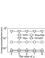
(b) HZ dataset

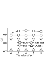
(c) CD dataset

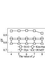
(d) HZ dataset

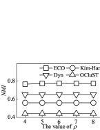
(e) CD dataset

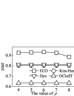
(f) HZ dataset

Figure 5. Effects of varying $\mathbf{\rho}$

6.2. Comparison and Parameter Study

We study the effect of parameters (summarized in Table 2) on the performance of the four methods.

Effects of varying $\bm{\rho}$

Figure 5 reports on the effect of varying $\delta$. First, ECO generally outperforms the baselines in terms of all performance metrics. In particular, ECO’s average processing time is almost one order of magnitude lower than Kim-Han and almost two orders of magnitude better than that of Dyn on both datasets. Moreover, ECO is even slightly more efficient than OCluST, because the latter updates its data structure repeatedly for macro-clustering. The high efficiency and quality of ECO are mainly due to three reasons: (i) Except for the initialization, ECO excludes iterative processes and is accelerated by grid indexing and the proposed optimizing techniques; (ii) ECO takes into account temporal smoothness, which is designed specifically for trajectories (cf. Formula 6); (iii) Locations with the potential to incur mutation of a clustering are adjusted to be closer to their neighbors that evolve smoothly, generally increasing the intra-density and decreasing the inter-density of clustering.

Second, we consider the effects of varying $\rho$. Figures 5a and 5b show that the average processing time is relatively stable. This is because the most time-consuming process in ECO is the clustering, which depends highly on the volume of data arriving at each time step. All four methods achieve higher efficiency on HZ than CD, due to CD’s larger average data size of each time step. Figures 5c–5f show that as $\rho$ grows, QS and NMI first increase and then drop. On the one hand, trajectories with high local density are generally more stable, i.e., more likely to remain in the same cluster in adjacent time steps. On the other hand, with a too large $\rho$, few minimal groups are generated, and thus few locations are smoothed. As the baselines do not have parameter $\rho$, their performance is unaffected.

Effects of varying $\bm{\delta}$

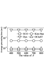
(a) CD dataset

(b) HZ dataset

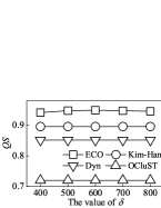
(c) CD dataset

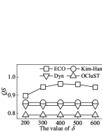
(d) HZ dataset

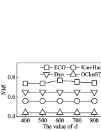
(e) CD dataset

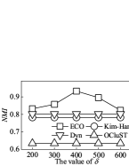
(f) HZ dataset

Figure 6. Effects of varying $\mathbf{\delta}$

Figure 6 reports in the effects of varying $\delta$. Specifically, ECO outperforms the baselines in terms of all metrics, and the processing times of the methods remain stable, as shown in Figures 6a and 6b. Figures 6c–6f indicate that as $\delta$ increases, both QS and NMI first increase and then drop. On the one hand, a too small $\delta$ leads to a small number of trajectories forming minimal groups and being smoothed; on the other hand, a too large $\delta$ also leads to few smoothing operations, as more pairs of trajectories $o$ and $o^{\prime}$ ($o,o^{\prime}\in\mathcal{M}_{k-1}(\tilde{s})$) satisfy $d(o.l,o^{\prime}.l)\leq\delta$ at $\textit{dt}_{k}$. Since the baselines do not utilize parameter $\delta$, they are unaffected by variations in $\delta$.

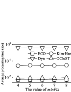
(a) CD dataset

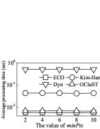
(b) HZ dataset

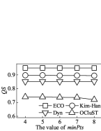
(c) CD dataset

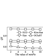
(d) HZ dataset

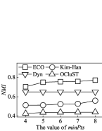
(e) CD dataset

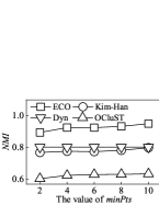
(f) HZ dataset

Figure 7. Effects of varying minPts

Effects of varying minPts

Figure 7 shows the effect of minPts on clustering. When varying minPts, the effects are similar to those seen when varying $\rho$ and $\delta$. Figures 7c and 7d show that QS of ECO, Dyn, and OCluST drop as minPts increases. The findings indicate that the average distance between trajectories in different clusters decreases with minPts. Assume that $o$ is a core point when minPts is small and that $o^{\prime}$ is a border point that is density reachable from $o$. As minPts increases, $o$ may no longer be a core point. In this case, $o^{\prime}$ and $o$ may be density reachable from different core points and may thus be in different clusters, even if $d(o.l,o^{\prime}.l)\leq\varepsilon$. As a result, the distances between trajectories in different clusters decrease. Figures 7e and 7f show that NMI increases with minPts for ECO, Dyn, and OCluST. The findings suggest that with a smaller minPts, the trajectories at the ”border” of a cluster are more likely to shift between being core points and being non-core points over time. In this case, clusters fluctuate more between consecutive time steps for a smaller minPts. As Dyn adopts particle swarm clustering instead of density based clustering, Dyn is unaffected by minPts.

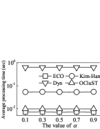
(a) CD dataset

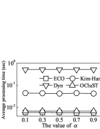
(b) HZ dataset

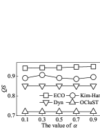
(c) CD dataset

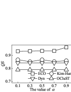
(d) HZ dataset

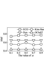
(e) CD dataset

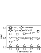
(f) HZ dataset

Figure 8. Effects of varying $\alpha$

Effects of varying $\bm{\alpha}$

Figure 8 shows the effects of varying $\alpha$. First, ECO always achieves the best performance among all methods. Second, all methods exhibit stable performance when varying $\alpha$. Third, both QS and NMI of ECO increase with $\alpha$. On the one hand, according to Formula 4.1, a larger $\alpha$ generally leads to a smaller distance between two trajectories in the same cluster. On the other hand, Formula 4.1 reduces the historical cost as $\alpha$ increases, which renders the evolution of clusters more smooth.

6.3. Scalability

To study the scalability, we vary the data size from 20% to 100%, which is done by randomly sampling moving objects by their IDs. The results are reported in Figure 9. First, ECO achieves the highest efficiency for large datasets, but is less efficient than OCluST for small datasets. This is because the locations of trajectories are generally distributed uniformly when data size is small. In this case, the grid index becomes less useful. As expected, the processing times of all methods increase with the dataset size.

Second, QS improves with the data size for all methods, with ECO always being best. As illustrated above, data distribution is generally non-uniform for a 100% dataset and becomes increasingly uniform as the data size decreases. Thus, the average distances between any pair of trajectories in the same cluster become smaller as data size increases, resulting in a larger QS.

Third, ECO achieves the highest NMI, which increases with the data size. This is mainly because fewer trajectories are able to form minimal groups and be subjected to smoothing when the average distances between any pair of trajectories increases.

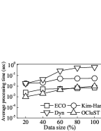
(a) CD dataset

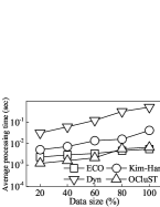
(b) HZ dataset

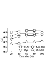
(c) CD dataset

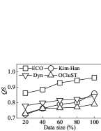
(d) HZ dataset

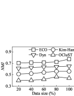
(e) CD dataset

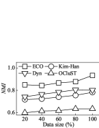
(f) HZ dataset

Figure 9. Scalability

7. Related Work

We proceed to review related works on streaming trajectory clustering and evolutionary clustering.

7.1. Streaming Trajectory Clustering

Streaming trajectory clustering finds representative paths or common movement trends among objects in real time. The main target of existing studies of streaming trajectory clustering is to update clusters continuously with high efficiency. Jensen et al. (Jensen et al., 2007) exploit an incrementally maintained clustering feature CF and propose a scheme for continuous clustering of moving objects. Costa et al. (Costa et al., 2014) define a new metric for streaming trajectory clustering and process trajectories by means of non-separable Fourier transforms. Tra-POPTICS (Deng et al., 2015) explores the use of graphics processing units to improve efficiency. Similar to ECO, proposals in  (Yu et al., 2013b; Yu et al., 2013a) use an index structure, TC-tree, to facilitate efficient updates of clusters. Some studies maintain a micro-group structure, that stores compact summaries of trajectories to enable fast and flexible clustering (Li et al., 2010; Da Silva et al., 2016; Mao et al., 2018; Riyadh et al., 2017). CUTis (Da Silva et al., 2016) continuously merges micro-groups into clusters, while CC_TRS (Riyadh et al., 2017), TCMM (Li et al., 2010), and OCluST (Mao et al., 2018) generate macro groups on top of micro groups when requested by users. In the experimental study, we compare with the state-of-the-art streaming trajectory clustering method (Mao et al., 2018). Some studies of real-time co-movement pattern mining also involve streaming trajectory clustering (Chen et al., 2019; Tang et al., 2012; Li et al., 2012). Comprehensive surveys of trajectory clustering are available (Bian et al., 2018; Yuan et al., 2017).

To the best of our knowledge, no existing studies of streaming trajectory clustering exploit temporal smoothness to improve clustering quality.

7.2. Evolutionary Clustering

Evolutionary clustering has been studied to discover evolving community structures in applications such as social (Kim and Han, 2009) and financial networks (Fenn et al., 2009) and recommender systems (Chen et al., 2020). Most studies target $k$-means, agglomerative hierarchical, and spectural clustering (Chakrabarti et al., 2006; Xu et al., 2014; Chi et al., 2007; Ma and Dong, 2017; Ma et al., 2019). Chakrabarti et al.  (Chakrabarti et al., 2006) propose a generic framework for evolutionary clustering. Chi et al. (Chi et al., 2007) develop two functions for evaluating historical costs, PCQ (Preserving Cluster Quality) and PCM (Preserving Cluster Membership), to improve the stability of clustering. Xu et al. (Xu et al., 2014) estimate the optimal smoothing parameter $\alpha$ of evolutionary clustering. Recent studies model evolutionary clustering as a multi-objective problem (Folino and Pizzuti, 2013; Yin et al., 2021; Liu et al., 2020, 2019) and use genetic algorithms to solve it, which is too expensive for online scenarios. Dyn (Yin et al., 2021), the state-of-the-art proposal, features non-redundant random walk based population initialization and an improved particle swarm algorithm to enhance clustering quality.

The Kim-Han proposal (Kim and Han, 2009) is the one that is closest to ECO. It uses neighbor-based smoothing and a cost embedding technique that smooths the similarity between each pair of nodes. However, ECO differs significantly from Kim-Han. First, the cost functions used are fundamentally different. Kim-Han’s cost function is designed specifically for nodes in dynamic networks and is neither readily applicable to, or suitable for, trajectory data. In contrast, ECO’s cost function is shaped according to the characteristics of the movements of trajectories. Second, Kim-Han smooths the similarity between each pair of neighboring nodes; in contrast, ECO smooths only the locations of a trajectory with abrupt movements, and the smoothing is performed only according to its most smoothly moving neighbor. Finally, Kim-Han includes iterative processes that degrade its efficiency, while ECO achieves $O(\lvert\mathcal{O}_{k}\rvert^{2})$ complexity at each time step in the worst case and adopts a grid index to improve efficiency.

8. Conclusion and Future Work

We propose a new framework for evolutionary clustering of streaming trajectories that targets faster and better clustering. Following existing studies, we propose so-called snapshot and historical costs for trajectories, and formalize the problem of evolutionary clustering of streaming trajectories, called ECO. Then, we formulate ECO as an optimization problem and prove that it can be solved approximately in linear time, which eliminates the iterative processes employed in previous proposals and improves efficiency significantly. Further, we propose a minimal group structure and a seed point shifting strategy that facilitate temporal smoothing. We also present the algorithms necessary to enable evolutionary clustering along with a set of optimization techniques that aim to enhance performance. Extensive experiments with two real-life datasets show that ECO outperforms existing state-of-the-art proposals in terms of clustering quality and running time efficiency.

In future research, it is of interest to deploy ECO on a distributed platform and to exploit more information for smoothing such as road conditions and driver preferences.

References

- (1)
- Bian et al. (2018) Jiang Bian, Dayong Tian, Yuanyan Tang, and Dacheng Tao. 2018. A survey on trajectory clustering analysis. arXiv preprint arXiv:1802.06971 (2018).
- Chakrabarti et al. (2006) Deepayan Chakrabarti, Ravi Kumar, and Andrew Tomkins. 2006. Evolutionary clustering. In SIGKDD. 554–560.
- Chen et al. (2020) Jianrui Chen, Chunxia Zhao, Lifang Chen, et al. 2020. Collaborative filtering recommendation algorithm based on user correlation and evolutionary clustering. Complex Syst. 6, 1 (2020), 147–156.
- Chen et al. (2019) Lu Chen, Yunjun Gao, Ziquan Fang, Xiaoye Miao, Christian S Jensen, and Chenjuan Guo. 2019. Real-time distributed co-movement pattern detection on streaming trajectories. PVLDB 12, 10 (2019), 1208–1220.
- Chi et al. (2007) Yun Chi, Xiaodan Song, Dengyong Zhou, Koji Hino, and Belle L Tseng. 2007. Evolutionary spectral clustering by incorporating temporal smoothness. In SIGKDD. 153–162.
- Costa et al. (2014) Gianni Costa, Giuseppe Manco, and Elio Masciari. 2014. Dealing with trajectory streams by clustering and mathematical transforms. Int. J. Intell. Syst. 42, 1 (2014), 155–177.
- Da Silva et al. (2016) Ticiana L Coelho Da Silva, Karine Zeitouni, and José AF de Macêdo. 2016. Online clustering of trajectory data stream. In MDM, Vol. 1. IEEE, 112–121.
- Deng et al. (2015) Ze Deng, Yangyang Hu, Mao Zhu, Xiaohui Huang, and Bo Du. 2015. A scalable and fast OPTICS for clustering trajectory big data. Cluster Comput 18, 2 (2015), 549–562.
- Ester et al. (1996) Martin Ester, Hans-Peter Kriegel, Jörg Sander, Xiaowei Xu, et al. 1996. A density-based algorithm for discovering clusters in large spatial databases with noise. In KDD, Vol. 96. 226–231.
- Fenn et al. (2009) Daniel J Fenn, Mason A Porter, Mark McDonald, Stacy Williams, Neil F Johnson, and Nick S Jones. 2009. Dynamic communities in multichannel data: An application to the foreign exchange market during the 2007–2008 credit crisis. J Nonlinear Sci 19, 3 (2009), 033119.
- Folino and Pizzuti (2013) Francesco Folino and Clara Pizzuti. 2013. An evolutionary multiobjective approach for community discovery in dynamic networks. TKDE 26, 8 (2013), 1838–1852.
- Gan and Tao (2017) Junhao Gan and Yufei Tao. 2017. Dynamic density based clustering. In SIGMOD. 1493–1507.
- Gupta et al. (2011) Manish Gupta, Charu C Aggarwal, Jiawei Han, and Yizhou Sun. 2011. Evolutionary clustering and analysis of bibliographic networks. In ASONAM. IEEE, 63–70.
- Idrissov and Nascimento (2012) Agzam Idrissov and Mario A Nascimento. 2012. A trajectory cleaning framework for trajectory clustering. In MDC workshop. 18–19.
- Jensen et al. (2007) Christian S Jensen, Dan Lin, and Beng Chin Ooi. 2007. Continuous clustering of moving objects. TKDE 19, 9 (2007), 1161–1174.
- Kim and Han (2009) Min-Soo Kim and Jiawei Han. 2009. A particle-and-density based evolutionary clustering method for dynamic networks. PVLDB 2, 1 (2009), 622–633.
- Li et al. (2020a) Lun Li, Xiaohang Chen, Qizhi Liu, and Zhifeng Bao. 2020a. A Data-Driven Approach for GPS Trajectory Data Cleaning. In DASFAA. Springer, 3–19.
- Li et al. (2021) Tianyi Li, Lu Chen, Christian S Jensen, and Torben Bach Pedersen. 2021. TRACE: real-time compression of streaming trajectories in road networks. PVLDB 14, 7 (2021), 1175–1187.
- Li et al. (2020b) Tianyi Li, Ruikai Huang, Lu Chen, Christian S Jensen, and Torben Bach Pedersen. 2020b. Compression of uncertain trajectories in road networks. PVLDB 13, 7 (2020), 1050–1063.
- Li et al. (2012) Xiaohui Li, Vaida Ceikute, Christian S Jensen, and Kian-Lee Tan. 2012. Effective online group discovery in trajectory databases. TKDE 25, 12 (2012), 2752–2766.
- Li et al. (2010) Zhenhui Li, Jae-Gil Lee, Xiaolei Li, and Jiawei Han. 2010. Incremental clustering for trajectories. In DASFAA. Springer, 32–46.
- Liu et al. (2020) Fanzhen Liu, Jia Wu, Shan Xue, Chuan Zhou, Jian Yang, and Quanzheng Sheng. 2020. Detecting the evolving community structure in dynamic social networks. World Wide Web 23, 2 (2020), 715–733.
- Liu et al. (2019) Fanzhen Liu, Jia Wu, Chuan Zhou, and Jian Yang. 2019. Evolutionary community detection in dynamic social networks. In IJCNN. IEEE, 1–7.
- Ma and Dong (2017) Xiaoke Ma and Di Dong. 2017. Evolutionary nonnegative matrix factorization algorithms for community detection in dynamic networks. TKDE 29, 5 (2017), 1045–1058.
- Ma et al. (2019) Xiaoke Ma, Dongyuan Li, Shiyin Tan, and Zhihao Huang. 2019. Detecting evolving communities in dynamic networks using graph regularized evolutionary nonnegative matrix factorization. Physica A 530 (2019), 121279.
- Mao et al. (2018) Jiali Mao, Qiuge Song, Cheqing Jin, Zhigang Zhang, and Aoying Zhou. 2018. Online clustering of streaming trajectories. Front. Comput. Sci. 12, 2 (2018), 245–263.
- Patil et al. (2018) Vikram Patil, Priyanka Singh, Shivam Parikh, and Pradeep K Atrey. 2018. GeoSClean: Secure cleaning of GPS trajectory data using anomaly detection. In MIPR. IEEE, 166–169.
- Riyadh et al. (2017) Musaab Riyadh, Norwati Mustapha, Md Sulaiman, Nurfadhlina Binti Mohd Sharef, et al. 2017. CC_TRS: Continuous Clustering of Trajectory Stream Data Based on Micro Cluster Life. Math. Probl. Eng. 2017 (2017).
- Song et al. (2015) Shaoxu Song, Chunping Li, and Xiaoquan Zhang. 2015. Turn waste into wealth: On simultaneous clustering and cleaning over dirty data. In SIGKDD. 1115–1124.
- Strehl and Ghosh (2002) Alexander Strehl and Joydeep Ghosh. 2002. Cluster ensembles—a knowledge reuse framework for combining multiple partitions. J Mach Learn Res 3, Dec (2002), 583–617.
- Tang et al. (2012) Lu-An Tang, Yu Zheng, Jing Yuan, Jiawei Han, Alice Leung, Chih-Chieh Hung, and Wen-Chih Peng. 2012. On discovery of traveling companions from streaming trajectories. In ICDE. IEEE, 186–197.
- Wang et al. (2020) Jiachuan Wang, Peng Cheng, Libin Zheng, Chao Feng, Lei Chen, Xuemin Lin, and Zheng Wang. 2020. Demand-aware route planning for shared mobility services. PVLDB 13, 7 (2020), 979–991.
- Wang et al. (2021) Sheng Wang, Yuan Sun, Christopher Musco, and Zhifeng Bao. 2021. Public Transport Planning: When Transit Network Connectivity Meets Commuting Demand. In SIGMOD. 1906–1919.
- Wu et al. (2015) Hao Wu, Chuanchuan Tu, Weiwei Sun, Baihua Zheng, Hao Su, and Wei Wang. 2015. GLUE: a parameter-tuning-free map updating system. In CIKM. 683–692.
- Xu et al. (2014) Kevin S Xu, Mark Kliger, and Alfred O Hero III. 2014. Adaptive evolutionary clustering. Data Min Knowl Discov 28, 2 (2014), 304–336.
- Yin et al. (2021) Ying Yin, Yuhai Zhao, He Li, and Xiangjun Dong. 2021. Multi-objective evolutionary clustering for large-scale dynamic community detection. Inf. Sci. 549 (2021), 269–287.
- Yu et al. (2013a) Yanwei Yu, Qin Wang, and Xiaodong Wang. 2013a. Continuous clustering trajectory stream of moving objects. China Commun. 10, 9 (2013), 120–129.
- Yu et al. (2013b) Yanwei Yu, Qin Wang, Xiaodong Wang, Huan Wang, and Jie He. 2013b. Online clustering for trajectory data stream of moving objects. Comput. Sci. Inf. Syst. 10, 3 (2013), 1293–1317.
- Yuan et al. (2017) Guan Yuan, Penghui Sun, Jie Zhao, Daxing Li, and Canwei Wang. 2017. A review of moving object trajectory clustering algorithms. ARTIF INTELL REV 47, 1 (2017), 123–144.
- Zeng et al. (2019) Yuxiang Zeng, Yongxin Tong, and Lei Chen. 2019. Last-mile delivery made practical: An efficient route planning framework with theoretical guarantees. PVLDB 13, 3 (2019), 320–333.