Low-J CO Line Ratios From Single Dish CO Mapping Surveys and PHANGS–ALMA

Abstract

We measure the low-$J$ CO line ratio $R_{21}\equiv\textup{CO}\,(2{\scalebox{0.75}[1.0]{$-$}}1)/\textup{CO}\,(1{\scalebox{0.75}[1.0]{$-$}}0)$, $R_{32}\equiv\textup{CO}\,(3{\scalebox{0.75}[1.0]{$-$}}2)/\textup{CO}\,(2{\scalebox{0.75}[1.0]{$-$}}1)$, and $R_{31}\equiv\textup{CO}\,(3{\scalebox{0.75}[1.0]{$-$}}2)/\textup{CO}\,(1{\scalebox{0.75}[1.0]{$-$}}0)$ using whole-disk CO maps of nearby galaxies. We draw CO $(2{\scalebox{0.75}[1.0]{$-$}}1)$ from PHANGS–ALMA, HERACLES, and follow-up IRAM surveys; CO $(1{\scalebox{0.75}[1.0]{$-$}}0)$ from COMING and the Nobeyama CO Atlas of Nearby Spiral Galaxies; and CO $(3{\scalebox{0.75}[1.0]{$-$}}2)$ from the JCMT NGLS and APEX LASMA mapping. Altogether this yields $76$, $47$, and $29$ maps of $R_{21}$, $R_{32}$, and $R_{31}$ at $20^{\prime\prime}\sim 1.3$ kpc resolution, covering $43$, $34$, and $20$ galaxies. Disk galaxies with high stellar mass, $\log(M_{\star}/\textrm{M}_{\odot})=10.25{-}11$ and star formation rate, $\mbox{{SFR}}=1{-}5$ M${}_{\odot}$ yr${}^{-1}$, dominate the sample. We find galaxy-integrated mean values and $16\%{-}84\%$ range of $R_{21}=0.65\ (0.50{-}0.83)$, $R_{32}=0.50\ (0.23{-}0.59)$, and $R_{31}=0.31\ (0.20{-}0.42)$. We identify weak trends relating galaxy-integrated line ratios to properties expected to correlate with excitation, including $\mbox{{SFR}}/M_{\star}$ and $\mbox{{SFR}}/L_{\rm CO}$. Within galaxies, we measure central enhancements with respect to the galaxy-averaged value of ${\sim}0.18^{+0.09}_{-0.14}$ dex for $R_{21}$, $0.27^{+0.13}_{-0.15}$ dex for $R_{31}$, and $0.08^{+0.11}_{-0.09}$ dex for $R_{32}$. All three line ratios anti-correlate with galactocentric radius and positively correlate with the local star formation rate surface density and specific star formation rate, and we provide approximate fits to these relations. The observed ratios can be reasonably reproduced by models with low temperature, moderate opacity, and moderate densities, in good agreement with expectations for the cold ISM. Because the line ratios are expected to anti-correlate with the CO $(1{\scalebox{0.75}[1.0]{$-$}}0)$-to-H${}_{2}$ conversion factor, $\alpha_{\rm CO}^{1-0}$, these results have general implications for the interpretation of CO emission from galaxies.

1 Introduction

Rotational line emission from carbon monoxide (CO) represents the main way to trace the distribution, kinematics, and physical conditions in the molecular interstellar medium in external galaxies (ISM, e.g., see reviews by BOLATTO13B; KLESSEN16). After several decades focused primarily on the fundamental ${}^{12}\textup{CO}\,(1{\scalebox{0.75}[1.0]{$-$}}0)$ transition at $\nu\approx 115$ GHz (e.g., YOUNG91; YOUNG95; HELFER03), improvements in (sub)millimeter facilities over the last fifteen years have enabled extensive mapping of nearby galaxies in ${}^{12}$CO $(2{\scalebox{0.75}[1.0]{$-$}}1)$ and ${}^{12}$CO $(3{\scalebox{0.75}[1.0]{$-$}}2)$ at $\nu\approx 231$ GHz and $\nu\approx 345$ GHz (e.g., LEROY09; WILSON12). In the last decade, the Atacama Large Millimeter/submillimeter Array (ALMA) has come online and revolutionized our view of molecular line emission from galaxies, while also accelerating the trend towards observing multiple CO lines. Thanks to its excellent site and submillimeter sensitivity, ALMA can often map CO $(2{\scalebox{0.75}[1.0]{$-$}}1)$ and CO $(3{\scalebox{0.75}[1.0]{$-$}}2)$ several times faster than CO $(1{\scalebox{0.75}[1.0]{$-$}}0)$ at matched resolution and sensitivity. As a result, ALMA surveys of nearby galaxies have targeted all three low-$J$ CO lines, CO $(3{\scalebox{0.75}[1.0]{$-$}}2)$, CO $(2{\scalebox{0.75}[1.0]{$-$}}1)$, and CO $(1{\scalebox{0.75}[1.0]{$-$}}0)$(e.g., GARCIABURILLO14; HIROTA18; LEROY21b).

Meanwhile, studies of redshifted CO emission have also become common, tracing the molecular gas at earlier cosmic epochs. Driven by similar technical considerations, these studies currently focus on CO $(3{\scalebox{0.75}[1.0]{$-$}}2)$, CO $(2{\scalebox{0.75}[1.0]{$-$}}1)$ or even higher $J$ transitions (e.g., see reviews by CARILLI13; HODGE20; TACCONI20). In the near future, observations at high redshift may become even more diverse as the proposed next generation Very Large Array (ngVLA; MURPHY18) will vastly improve our ability to observe CO $(1{\scalebox{0.75}[1.0]{$-$}}0)$ emission at intermediate and high redshift.

This increased diversity of CO line observations at low and high $z$ makes the ability to translate between results obtained using these different CO lines crucial. Despite the proliferation of CO $(2{\scalebox{0.75}[1.0]{$-$}}1)$ and CO $(3{\scalebox{0.75}[1.0]{$-$}}2)$ studies, many surveys still target CO $(1{\scalebox{0.75}[1.0]{$-$}}0)$, including xCOLD GASS (SAINTONGE17) and CARMA EDGE (BOLATTO17), the largest low-$z$ single dish and interferometric CO surveys to date. Critical work informing our interpretation of CO emission has also built on observations of a single transition, e.g., DONOVANMEYER13 focused on CO $(1{\scalebox{0.75}[1.0]{$-$}}0)$ emission, SANDSTROM13 studied CO $(2{\scalebox{0.75}[1.0]{$-$}}1)$, and WILSON08 employed CO $(3{\scalebox{0.75}[1.0]{$-$}}2)$. Well-understood, observationally-tested translations between the various low-$J$ CO lines are required to link these efforts.

Indeed, translations between the different transitions are not straightforward because the ratios among CO $(3{\scalebox{0.75}[1.0]{$-$}}2)$, CO $(2{\scalebox{0.75}[1.0]{$-$}}1)$, and CO $(1{\scalebox{0.75}[1.0]{$-$}}0)$ also reflect physical conditions in the molecular gas. The observed ratios emerge from an interplay among the distributions of collider density, kinetic temperature, $T_{\textrm{kin}}$, and column density per line width (see §2). These in turn depend on the structure, kinematics, and heating mechanisms at play in the cold ISM. The ratios of low-$J$ CO lines thus represent a potentially powerful observational probe of the local physical conditions in the molecular ISM. This potential is complicated by degeneracies in their interpretation and the modest dynamic range in their observed values. This limited dynamic range places relatively strict requirements on observations aiming to measure these line ratios.

In contrast to commonly used “dense gas tracers” like HCN $(1{\scalebox{0.75}[1.0]{$-$}}0)$ and HCO${}^{+}\,(1{\scalebox{0.75}[1.0]{$-$}}0)$, the CO lines are bright and can be studied across a range of environments (see USERO15, regarding relative line strengths). Numerical simulations can now resolve CO chemistry and predict CO line emission over whole molecular clouds, large parts of a spiral galaxy, or even entire dwarf galaxies (e.g., GLOVER12; PENAZOLA17; PENALOZA18; GONG20; HU21), but such calculations remain extremely challenging for tracers of higher density gas (e.g., ONUS18). A combined observational, numerical, and analytic approach that leverages ratios among the low-$J$ CO lines and their isotopologues represents a promising path forward to diagnose physical conditions in the molecular gas of galaxies. This approach can become even more powerful when paired with high resolution imaging of the CO emission (e.g., see GALLAGHER18B), which places constraints on the mean density and kinematics of the cold gas (e.g., see SUN18; SUN20B; ROSOLOWSKY21). Of course, spectroscopy targeting multiple CO transitions or CO isotopologues has a long history (e.g., PAPADOPOULOS99; ISRAEL01; ISRAEL03; ISRAEL15; BAYET04; BAYET06; KAMENETZKY14; KAMENETZKY17). However, most previous work has focused on single-pointing or galaxy-integrated measurements, with a heavy emphasis on galaxy centers and starburst galaxies, including many ultraluminous and luminous infrared galaxies (U/LIRGs). Resolved studies that measure the ratios among multiple CO lines over the full area of “normal” star-forming main sequence galaxies remain relatively scarce.

This paper presents new measurements of the $\textup{CO}\,(2{\scalebox{0.75}[1.0]{$-$}}1)/\textup{CO}\,(1{\scalebox{0.75}[1.0]{$-$}}0)$, $\textup{CO}\,(3{\scalebox{0.75}[1.0]{$-$}}2)/\textup{CO}\,(2{\scalebox{0.75}[1.0]{$-$}}1)$, and $\textup{CO}\,(3{\scalebox{0.75}[1.0]{$-$}}2)/\textup{CO}\,(1{\scalebox{0.75}[1.0]{$-$}}0)$ line ratios for nearby galaxies ($D<40$ Mpc, median $\sim 14$ Mpc) based on maps of CO emission from KUNO07, HERACLES (LEROY09), the JCMT NGLS (WILSON12), COMING (SORAI19), PHANGS–ALMA (LEROY21b), new IRAM 30-m CO $(2{\scalebox{0.75}[1.0]{$-$}}1)$ observations (P.I. A. Schruba), and new APEX LASMA CO $(3{\scalebox{0.75}[1.0]{$-$}}2)$ observations (P.I. A. Weiss). We measure both resolved and integrated CO line ratios using mapping surveys. All of these surveys except PHANGS–ALMA use receiver arrays on single dish telescopes to cover large areas quickly (e.g., see SCHUSTER07). Restricting our focus to mapping data allows us to construct identical matched apertures when measuring integrated ratios. This avoids the common issue of mismatched beams, which plagued some earlier studies that relied on pointed observations. These surveys also target many of the largest, closest, best studied galaxies, so the ratios for individual targets are of particular interest. Finally, because we analyze maps, we can measure line ratios associated with distinct regions to, e.g., test for a dependence of excitation on galactocentric radius or star formation rate surface density (e.g., following DENBROK21; YAJIMA21).

LEROY09, WILSON12, and LEROY13 calculated these ratios based on first versions of HERACLES and the JCMT NGLS, and YAJIMA21 have recently combined HERACLES and COMING. But the number and quality of CO maps of galaxies have grown significantly compared to any study currently in the literature, particularly with the release of PHANGS–ALMA. Quite a few studies have examined these ratios in individual galaxies and noted local variations in individual ratios (e.g., CROSTHWAITE07; KODA12; VLAHAKIS13; UEDA12; DRUARD14; LAW18; KODA20), but so far there has been relatively little attempt to synthesize these mapping measurements (though see the beam-matched, single-pointing measurements by SAINTONGE17; LAMPERTI20).

As a practical matter, we present our study in the context of the PHANGS–ALMA CO $(2{\scalebox{0.75}[1.0]{$-$}}1)$ survey. PHANGS–ALMA mapped CO $(2{\scalebox{0.75}[1.0]{$-$}}1)$ across $90$ nearby galaxies at ${\lesssim}150$ pc resolution. To aid in the interpretation of these data, we also aim to improve our empirical understanding of the $\textup{CO}\,(2{\scalebox{0.75}[1.0]{$-$}}1)/\textup{CO}\,(1{\scalebox{0.75}[1.0]{$-$}}0)$ and $\textup{CO}\,(3{\scalebox{0.75}[1.0]{$-$}}2)/\textup{CO}\,(2{\scalebox{0.75}[1.0]{$-$}}1)$ ratios. Ultimately, we expect this to improve our ability to estimate the molecular mass and infer an appropriate CO-to-H${}_{2}$ conversion factor for these data. This work complements three other recent or forthcoming studies. DENBROK21 use $9$ new, high quality $22^{\prime\prime}$ resolution CO $(1{\scalebox{0.75}[1.0]{$-$}}0)$ maps from the IRAM 30-m telescope to investigate the resolved $\textup{CO}\,(2{\scalebox{0.75}[1.0]{$-$}}1)/\textup{CO}\,(1{\scalebox{0.75}[1.0]{$-$}}0)$ ratio. This work also complements the study by T. Saito et al. (in preparation), which investigates the behavior of the CO $(2{\scalebox{0.75}[1.0]{$-$}}1)$/CO $(1{\scalebox{0.75}[1.0]{$-$}}0)$ ratio at higher $4{-}8^{\prime\prime}$ resolution in four PHANGS–ALMA targets. In scope, our study resembles the recent thorough investigation by YAJIMA21, but we take advantage of a larger database of CO $(2{\scalebox{0.75}[1.0]{$-$}}1)$ maps and include CO $(3{\scalebox{0.75}[1.0]{$-$}}2)$ in our analysis.

After framing some theoretical and observational expectations (§2), we describe the data that we use and our measurements (§3). Then we measure galaxy-integrated line ratios (§4.1) and compare them to galaxy’s integrated properties (§4.2). Then we examine the resolved behavior of the ratio as a function of galactocentric radius, local SFR, and stellar mass surface density (§LABEL:sec:local). Finally, we discuss the implications of our measurements and next steps (§LABEL:sec:discussion) and then summarize our results (§LABEL:sec:summary).

2 Expectations

Figure 1: CO line ratios produced by model calculations (gray points) with key trends illustrated. Predicted line ratios $R_{32}$ vs. $R_{21}$ for model calculations using RADEX (VANDERTAK07) and lognormal density distributions following LEROY17B. Each gray point shows an individual model. As described in Appendix LABEL:sec:comodels, each model is characterized by a kinetic temperature ($T_{\rm kin}$), a total CO column density per line width ($N_{\rm CO}/\Delta v$), a lognormal density distribution width ($\sigma$), and a mean H${}_{2}$ collider density ($n_{0}$). To illustrate how the line ratios change when varying density ($n_{0}$), temperature ($T_{\rm kin}$), and opacity (set by $N_{\rm CO}/\Delta v$) while holding other parameters fixed, a subset of the data is shown by colored lines for reference. Both panels show the same model grid using gray points while changing the reference. In the left panel, the colored lines show the effect of varying $N_{\rm CO}/\Delta v$, which sets opacity and escape probability, while holding temperature and density constant at a few representative values. In the right panel, dashed lines show the result of varying temperature ($T_{\rm kin}$), and solid lines show the results of varying the mean density ($n_{0}$) while holding $N_{\rm CO}/\Delta v$ fixed. For all reference lines, we fix $\sigma=0.6$ dex. Note that these lines are intended to be illustrative, not spanning the full phase space of the modeling. The full model grid spanning a plausible range of temperatures and densities is available as a machine readable table in Appendix LABEL:sec:comodels.

Throughout this paper, we refer to the line ratios as

$$\begin{split}R_{21}&\equiv I_{2-1}/I_{1-0}\\ R_{32}&\equiv I_{3-2}/I_{2-1}\\ R_{31}&\equiv I_{3-2}/I_{1-0}\end{split}$$ (1)

Here $I_{2-1}$, for example, refers to the velocity-integrated specific intensity of the CO $(2{\scalebox{0.75}[1.0]{$-$}}1)$ line, with analogous definitions for the other lines. All intensities, luminosities, and line ratios in this paper are calculated in Rayleigh–Jeans brightness temperature units. Line-integrated intensities are presented in K km s${}^{-1}$ and luminosities given in K km s${}^{-1}$ pc${}^{2}$.

In these “Kelvin” units, we expect a line ratio of $1$ for all ratios for an optically thick source in local thermodynamic equilibrium (LTE) when both transitions sit securely on the Rayleigh–Jeans tail given the source temperature, $T_{\rm kin}$. Note however, that under real conditions the Rayleigh–Jeans criterion, $h\nu\ll kT_{\rm kin}$, may not be satisfied. This will happen, for example considering emission in high frequency transitions from low temperature sources. When the Rayleigh–Jeans criterion is not met, because $T_{\rm kin}$ has low enough values relative to the frequencies of the observed transitions, this will drive the “thermal” value of the line ratio observed from an optically thick source to values below $1$. In Appendix LABEL:sec:corrections, we illustrate the expected opaque LTE value for the relevant ratios, and also show the effects of the cosmic microwave background. For purposes of reading the observational results in this paper, the key point is that at relevant temperatures, $T_{\rm kin}\sim 10{-}20$ K, the expected ratio for opaque, thermalized gas can be as low as ${\sim}0.7$.

Expectations from models: Theoretically, the observed line ratios depend on the distributions of temperature, $T_{\rm kin}$, collider density, $n_{\mathrm{H_{2}}}$, and column density of CO per line width in the gas, $N/\Delta v$. A full discussion of the interplay of these quantities with $R_{32}$, $R_{21}$, and $R_{31}$ lies beyond the scope of this work, and we refer the reader to BOLATTO13A, SHIRLEY15, LEROY17B, and PENALOZA17, each of which touches on some aspects of the topic.

As a brief summary, we illustrate the behavior of $R_{32}$ and $R_{21}$ in Figure 1, which plots results from a set of model calculations following LEROY17B. In the figure, each point shows the line ratios predicted from a model that has a lognormal distribution of collider densities described by a mean density, $n_{0}$, and a width, $\sigma$. Each model also has a single fixed $T_{\rm kin}$ and a single value of $N_{\rm CO}/\Delta v$, which we adopt for each individual density layer. We use RADEX (VANDERTAK07) with data from the Leiden Atomic and Molecular Database (LAMDA; SCHOIER05) to calculate predicted emission. The calculations generally follow LEROY17B with the distinction that here we fix $N_{\rm CO}/\Delta v$ rather than fixing the optical depth, $\tau$, of a particular line as in that paper. Because these exact calculations may be of general use and are not fully reported in LEROY17B, we report the model grid as a machine readable table in Appendix LABEL:sec:comodels.

Figure 1 illustrates the combined effects of temperature, density, and optical depth on the line ratios. In the left panel, each line shows fixed $T_{\rm kin}$ and a fixed density distribution, while we vary $N_{\rm CO}/\Delta v$, the total column density of CO molecules normalized to the line width. $N_{\rm CO}/\Delta v$ affects the optical depth and escape probability, and through these also affects the critical density and level populations. The figure shows how the low opacities yielded by low $N_{\rm CO}/\Delta v$ can lead to high, “super-thermal” line ratios with values $>1$ in the case of low opacity gas in LTE. Alternatively, for low density gas, low $N_{\rm CO}/\Delta v$ can yield very low line ratios, indicating sub-critically excited gas. Meanwhile higher $N_{\rm CO}/\Delta v$ tends to drive gas closer to optically thick LTE and towards line ratios of ${\sim}1$.

The right panel shows how at fixed $N_{\rm CO}/\Delta v$, the density distribution and temperature also play important roles. Their exact impact depends on the $N_{\rm CO}/\Delta v$. In general, higher density and higher temperature at fixed $N_{\rm CO}/\Delta v$ generally drive both ratios towards higher values. The variations for optically thin gas are more extreme, even allowing line ratios above $1$, while optically thicker gas shows more dynamic range in $R_{32}$ at the densities illustrated because of the higher excitation requirements of those transitions.

Expectations from previous observations: Previous observations establish some basic expectations for low-$J$ CO line ratios in nearby galaxies:

1. Normal star-forming galaxies show $R_{21}$ in the range ${\sim}0.4{-}0.9$ (e.g., LEROY13; DENBROK21; YAJIMA21). $R_{31}$ likely shows lower values, sometimes as low as ${\sim}0.2$, in normal galaxies (e.g., MAO10; WILSON12), but also a larger range of reported values (e.g., MAUERSBERGER99; MAO10; LAMPERTI20).

2. Starburst galaxies and active galaxies show higher, closer to thermal (i.e., ${\sim}1$) ratios (e.g., MAUERSBERGER99; WEISS05; MAO10; LAMPERTI20; YAJIMA21), consistent with having both higher densities and hotter gas.

3. The central parts of normal star-forming galaxies show systematically higher $R_{21}$ (e.g., BRAINE92; BRAINE93; LEROY09; LEROY13; ISRAEL20; DENBROK21; YAJIMA21), consistent with higher densities and hotter gas in the central parts of these galaxies (e.g., MANGUM13; SUN20B, among many others) and with observations showing high temperatures and densities in the center of our own Milky Way (e.g., AO13; GINSBURG16; KRIEGER17).

4. In addition to the contrast between normal galaxies and starbursts, and between disks and galaxy centers, there is statistical evidence that regions with hotter dust, higher star formation rate surface density, or shorter depletion times show higher line ratios within normal star-forming galaxies (e.g., LAMPERTI20; DENBROK21; YAJIMA21).

5. Given the modest dynamic range of the observed ratios and the need to combine multiple instruments, calibration uncertainties can imply significant scatter in line ratio measurements (see excellent discussions in DENBROK21; YAJIMA21). For single-pointing observations with single dish telescopes, uncertain aperture corrections also represent a significant source of uncertainty. These systematics, in addition to the limited sensitivity of mm-wave telescopes before ALMA, may help explain why many results in the literature show substantial scatter.

These general trends are largely born out by detailed studies of individual galaxies (e.g., KODA12; KODA20), though there remains disagreement in the literature about the behavior of the ratios, e.g., relative to spiral arms or within individual targets. Some of this may reflect that at high resolution, line ratios can show detailed variations that track the location of individual heating sources or vary across spiral arms and bars (e.g., UEDA12; LAW18, and T. Saito et al. in preparation).

3 Measurements

Figure 2: Consistency among galaxy-integrated CO fluxes in repeat observations. Each panel shows the ratio among the galaxy-integrated CO luminosity, $L_{\rm CO}$, estimated using different surveys targeting the same galaxy. Each point indicates one galaxy, with the error bar showing only statistical uncertainties. The $x$-axis shows the CO flux associated with the denominator (i.e., COMING or PHANGS-ALMA). A solid gray line in both panels indicates the expectation for perfect agreement and the shaded region and colored line show $\pm 1$ standard deviation about the median ratio. The NRO atlas shows $0.91$ times the CO luminosity of COMING, with $\pm 12\%$ robustly estimated scatter. Where the two samples overlap in this study, IRAM 30-m HERA mapping shows median $1.03$ times higher luminosity than PHANGS with $\pm 12\%$ robustly estimated scatter.

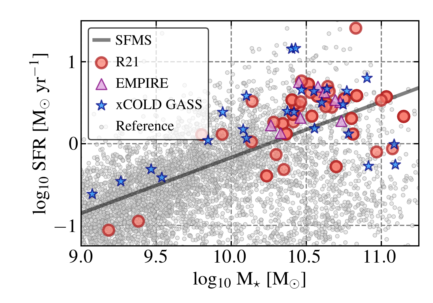
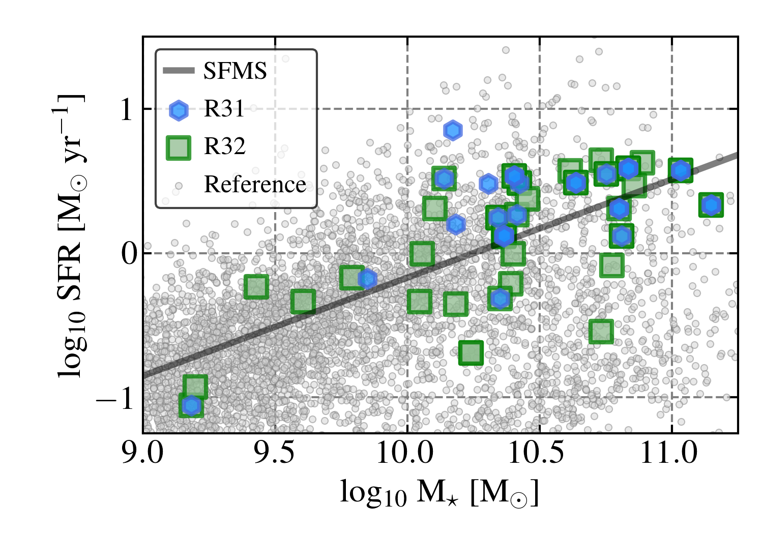
Figure 3: Galaxies with beam-matched line ratio measurements in SFR–$M_{\star}$ space. Location of our targets in SFR–$M_{\star}$ space, plotted over the larger sample of galaxies within $d<50$ Mpc with SFR and $M_{\star}$ calculated in a consistent way (LEROY19). The black line shows an estimate of the SFR–$M_{\star}$ relationship for local star-forming galaxies (LEROY19, in excellent agreement with CATINELLA18). Red circles, blue hexagons, and green squares show galaxies with measurements (not limits) in this paper, with the top panel showing galaxies with $R_{21}$ measured and the bottom panel showing $R_{32}$ and $R_{31}$. For comparison, we also plot the properties of EMPIRE targets from DENBROK21 and the $R_{21}$ properties of the subset of xCOLD GASS with beam-matched $R_{21}$ measurements from SAINTONGE17. Despite the relatively large number of measurements, our $R_{21}$ measurements remain highly clustered in this space, biased towards high-mass and high-SFR galaxies. The measurements involving the CO $(3{\scalebox{0.75}[1.0]{$-$}}2)$ line show slightly more homogeneous sampling of parameter space despite their overall lower number and higher typical uncertainty.

Table 1: Summary of map pairs in this paper.

Survey Pair	Sample Size
	(Meas./LL/UL)
$R_{21}\equiv\textup{CO}\,(2{\scalebox{0.75}[1.0]{$-$}}1)/\textup{CO}\,(1{\scalebox{0.75}[1.0]{$-$}}0)$
PHANGS–ALMA + COMING	10/1/0
PHANGS–ALMA + NRO Atlas	18/0/0
HERA + COMING	23/1/0
HERA + NRO Atlas	23/0/0
Total map pairs	76
Unique galaxies	43
$R_{32}\equiv\textup{CO}\,(3{\scalebox{0.75}[1.0]{$-$}}2)/\textup{CO}\,(2{\scalebox{0.75}[1.0]{$-$}}1)$
NGLS + PHANGS–ALMA	11/0/2
NGLS + HERA	22/0/5
APEX + PHANGS–ALMA	5/0/0
APEX + HERA	2/0/0
Total map pairs	47
Unique galaxies	34
$R_{31}\equiv\textup{CO}\,(3{\scalebox{0.75}[1.0]{$-$}}2)/\textup{CO}\,(1{\scalebox{0.75}[1.0]{$-$}}0)$
NGLS + COMING	13/0/1
NGLS + NRO Atlas	11/0/0
APEX + COMING	2/0/0
APEX + NRO Atlas	2/0/0
Total map pairs	29
Unique galaxies	20

Note. — Surveys: COMING is described by SORAI19. “NRO Atlas” refers to the survey presented by KUNO07. PHANGS–ALMA is described by LEROY21b. “HERA” refers to HERACLES (LEROY09; LEROY13) and a follow up Virgo Cluster survey (P.I. A. Schruba). “NGLS” refers to the JCMT survey by WILSON12 supplemented by a few follow-up or archival JCMT observations. “APEX” refers to APEX LASMA mapping by J. Puschnig et al. (in preparation).

Table 1 summarizes the survey combinations and targets for each line ratio. We use new CO $(2{\scalebox{0.75}[1.0]{$-$}}1)$ maps from the PHANGS–ALMA survey (LEROY21b), CO $(2{\scalebox{0.75}[1.0]{$-$}}1)$ maps from HERACLES on the IRAM 30-m telescope (LEROY09), and another set of IRAM 30-m CO $(2{\scalebox{0.75}[1.0]{$-$}}1)$ maps that cover mostly Virgo Cluster targets (A. Schruba et al. in preparation). We draw CO $(1{\scalebox{0.75}[1.0]{$-$}}0)$ maps from two Nobeyama 45-m surveys, the CO Multiline Imaging of Nearby Galaxies (COMING) Survey (SORAI19) and the Nobeyama CO Atlas of Nearby Spiral Galaxies (hereafter the “NRO Atlas”; KUNO07). We compare these to CO $(3{\scalebox{0.75}[1.0]{$-$}}2)$ maps from the JCMT Nearby Galaxy Legacy Survey (hereafter the NGLS; WILSON12) and from a new APEX LASMA mapping project (J. Puschnig et al. in preparation). In total, as summarized in Table 1 this leads to $152$ map pairs with $43$ unique galaxies mapped in both CO $(2{\scalebox{0.75}[1.0]{$-$}}1)$ and CO $(1{\scalebox{0.75}[1.0]{$-$}}0)$, $34$ mapped in CO $(3{\scalebox{0.75}[1.0]{$-$}}2)$ and CO $(2{\scalebox{0.75}[1.0]{$-$}}1)$, and $20$ mapped in CO $(3{\scalebox{0.75}[1.0]{$-$}}2)$ and CO $(1{\scalebox{0.75}[1.0]{$-$}}0)$. A total of $16$ unique galaxies have a measurement, not a limit, for all three lines.

To consider a line ratio measurement, we require that CO emission be securely detected in at least one transition, so that we can at least obtain a limit on the line ratio. For each target that meets this criterion, we estimate the integrated line ratios and compare these to the integrated properties of the galaxy. For targets with high enough signal-to-noise, we also measure the line ratio in individual $20^{\prime\prime}$ regions, with this $20^{\prime\prime}$ scale picked because it represents the common angular resolution achievable by all of the mapping surveys used in our analysis, with APEX LASMA being the limiting data set. The median distance to the target across all of our measurements is ${\sim}14$ Mpc, where this scale corresponds to ${\sim}1.3$ kpc, and the $16{-}84^{\rm th}$ percentile range of distance is 9 to 18 Mpc, implying physical beam sizes of ${\sim}0.9{-}1.8$ kpc. This resolution is typically sufficient to resolve the disk of the galaxy but not isolate individual molecular clouds or resolve features like spiral arms or bars. Using these measurements, we correlate the line ratios with local conditions in the galaxy disk, including galactocentric radius, $r_{\rm gal}$, local star formation rate surface density, $\Sigma_{\rm SFR}$, and stellar mass surface density, $\Sigma_{\star}$.

We make separate line ratio measurements for each galaxy and specific survey pair. This can lead to the case where we measure the same line ratio multiple times for a single galaxy, e.g., NGC 0628 appears in both HERACLES and PHANGS–ALMA. We use these duplicated observations to help assess the systematic uncertainty, confirming that key uncertainties in the field still often relate to calibration differences among telescopes (see below, Figure 2, and more discussion in DENBROK21). We report all line ratio pairs, but when searching for possible correlations and fitting scaling relations we adopt only a single value of a line ratio per galaxy, using the following priority: PHANGS–ALMA over HERACLES; COMING over the NRO Atlas; APEX over the JCMT NGLS.

Conventions: We correct all quoted surface densities for the effects of inclination. Our stellar mass and star formation rate maps assume a CHABRIER03 initial mass function (IMF) and are calibrated to be on the same scale as the GALEX–WISE–SDSS Legacy Survey (SALIM16; SALIM18).

3.1 CO data

Table 1 summarizes the sources of our line ratios, which come from combining data from ALMA, the IRAM 30-m telescope, the Nobeyama Radio Observatory (NRO) 45-m telescope, and the James Clerk Maxwell Telescope (JCMT). Specifically, we use the following individual surveys.

PHANGS–ALMA CO (2 $-$ 1) Data: LEROY21b describe the selection and observations of PHANGS–ALMA and LEROY21a describe the data processing, imaging, and data product creation. Here we use the combined interferometric and total power CO $(2{\scalebox{0.75}[1.0]{$-$}}1)$ cubes convolved to our common resolution of $20^{\prime\prime}$. These PHANGS–ALMA CO $(2{\scalebox{0.75}[1.0]{$-$}}1)$ data have median native resolution $1.3^{\prime\prime}$, much higher than our working resolution. Because they include total power data, as well as short spacing 7-m array data, we expect them to have the correct global flux scale and to be sensitive to extended emission, and so to be well-suited to this analysis after convolution. LEROY21b confirm an overall good agreement between the PHANGS–ALMA CO $(2{\scalebox{0.75}[1.0]{$-$}}1)$ and lower resolution single dish measurements, which we also show below.

ALMA provides a total power calibration based on regular monitoring of quasars, and the gain uncertainty associated with ALMA at these frequencies is nominally $5{-}10$%. We take $10\%$ as a conservative estimate, though we note that this likely overestimates the true uncertainty. In LEROY21a, we verified that the internal stability of the PHANGS–ALMA total power data appears very good, with fluxes repeatable at the ${\sim}3\%$ level from day-to-day. A few cubes do suffer from $2{-}7$% gain uncertainties due to issues described in LEROY21a. The PHANGS–ALMA data have extremely good sensitivity compared to the other data in this paper, but their field of view tends to be more limited than the other maps, with PHANGS–ALMA typically covering 70% of the total mid-IR emission from its target galaxy. As described in Section 3.4, we account for this issue in our analysis.

IRAM 30-m HERA CO (2 $-$ 1) Data: We also analyze CO $(2{\scalebox{0.75}[1.0]{$-$}}1)$ maps from HERACLES (LEROY09) and another $21$ galaxies observed by the IRAM 30-m telescope as part of a survey focused on the Virgo Cluster (P.I. Schruba; A. Schruba et al. in preparation). These new data were observed in a manner identical to HERACLES and reduced following the same procedures. Both data sets have native FWHM beam size of $13\farcs 3$ and large extent, usually covering out beyond the optical radius of the galaxy. The calibration uncertainty associated with the HERA data is ${<}20\%$ based on a detailed gain analysis presented in DENBROK21, a bootstrapping analysis in LEROY09, and comparing to PHANGS–ALMA (LEROY21b). This calibration uncertainty can also apply within maps, reflecting uneven gains among the receiver array. DENBROK21 note the two most extreme cases, NGC 3627 and NGC 5194, were both observed early in the life of the HERA instrument (SCHUSTER07) when observing procedures had not yet been optimized. To be conservative, we adopt a nominal uncertainty $20\%$, near the upper limit of the plausible calibration uncertainty. This adopted calibration uncertainty agrees with the consistency check shown in Figure 2 and the results of the checks in LEROY21b.

NRO CO (1 $-$ 0) Data: We utilize CO $(1{\scalebox{0.75}[1.0]{$-$}}0)$ maps obtained by the Nobeyama Radio Observatory from the CO Multi-line Imaging of Nearby Galaxies (COMING) survey (SORAI19). These data have native resolution $17^{\prime\prime}$ and cover large areas in each target. We also compare to CO $(1{\scalebox{0.75}[1.0]{$-$}}0)$ maps from the Nobeyama CO Atlas of Nearby Spiral Galaxies (“NRO Atlas”) presented by KUNO07. These have $15^{\prime\prime}$ resolution and higher sensitivity than COMING, but the KUNO07 data suffer from more visible mapping artifacts and poor baselines compared to SORAI19. Following YAJIMA21, we take the gain uncertainty for both data sets to be $25\%$, reflecting a combination of true calibration uncertainties and pointing errors. Similar to the HERA case noted above, these systematic uncertainties can apply within a galaxy, and do not only reflect an overall scaling from galaxy to galaxy.

JCMT CO (3 $-$ 2) Data: We also compare to maps of CO $(3{\scalebox{0.75}[1.0]{$-$}}2)$ emission from the JCMT NGLS (WILSON12) and individual galaxy follow-up programs (P.I. E. Rosolowsky) observed under projects M09BC15, M10BC06, and M12AC03. The follow-up program data were calibrated using the starlink software package (CURRIE14) using the observatory-recommended pipelines. The JCMT data initially had $14\farcs 5$ resolution. We convolved them to a resolution of $20^{\prime\prime}$ for further processing and translated them into the main beam temperature scale using an efficiency of $0.6$ at $345$ GHz (following WILSON12).

After this convolution, we inspected the data and found that they could be improved by fitting and subtracting low order baselines. For each line of sight, we defined a velocity range of interest based on the velocity range of CO emission seen in the other CO data for the galaxy. Specifically, we defined a reference cube used to define the baseline region, with the priority given to PHANGS–ALMA, then IRAM HERA data, then COMING data, then NRO Atlas data. Because the CO $(3{\scalebox{0.75}[1.0]{$-$}}2)$ data tend to have lower signal to noise than the lower-$J$ cubes, using the other cubes as a template to fit the baseline should be well-defined and impose little or no bias. Then, we considered each line of sight in the JCMT cube. Along that line of sight, we excluded velocities detected above $\mathrm{S/N}=3$ in either the reference CO cube or the JCMT data themselves from the fit, and focused the baseline fit on regions near the detected line emission. We defaulted to a $\pm 50$ km s${}^{-1}$ fitting window but adjusted this slightly from galaxy-to-galaxy. Then we fit and subtracted a baseline from each line of sight, using iterative outlier rejection of the JCMT data to refine the fit. We used an order $0$ fit, i.e., we subtracted the mean, for all galaxies except NGC 2403, where we used a linear fit. In a few galaxies, we also blanked regions of the JCMT cube that were clearly dominated by artifacts. Finally, after inspecting the data, we dropped a few potential targets where the data remained clearly dominated by artifacts despite our baseline fitting. By virtue of using the other CO data as a prior for baseline fits, we also effectively required that all JCMT targets were detected in another CO transition.

We lack a detailed characterization of the calibration and pointing uncertainty for the JCMT data, but according to the JCMT web pages the nominal calibration accuracy of the JCMT is 10% before accounting for uncertainties in pointing or sub-optimal conditions. Empirically, the integrated fluxes that we measure frequently vary by ${\gtrsim}10{-}20\%$ when we compare results before and after our rebaselining. We adopt an overall calibration uncertainty 20% as a conservative estimate, consistent with, e.g., YAJIMA21; SORAI19 for NRO and DENBROK21; LEROY09 for IRAM HERA maps. As with the IRAM HERA maps, we consider this to represent the upper envelope of plausible uncertainties.

APEX CO (3 $-$ 2) Data: We also compare to five maps of CO $(3{\scalebox{0.75}[1.0]{$-$}}2)$ emission obtained using the Large APEX Sub-Millimetre Array (LASMA) receiver array on the Atacama Pathfinder Experiment (APEX) telescope (GUESTEN08). LASMA is a seven pixel, single polarization array receiver that can observe from $\nu=268{-}375$ GHz. At the $\nu\approx 345$ GHz of CO $(3{\scalebox{0.75}[1.0]{$-$}}2)$, the array has a beam size of ${\sim}18.5^{\prime\prime}$. After reduction and convolution during gridding, these maps end up having a beam size of ${\sim}20^{\prime\prime}$, which sets the common resolution of our data. These maps were obtained as part of APEX projects m-0103.f-9520a-2019 and m-0104.f-9516a-2019 (PI: A. Weiss) and will be presented in detail in J. Puschnig et al. (in preparation). They target galaxies that have PHANGS–ALMA imaging, and the areal extent is designed to match that of the PHANGS–ALMA maps almost exactly. The final data cubes have been gridded to our common velocity resolution of 10 km s${}^{-1}$. At $20^{\prime\prime}$ resolution and with 10 km s${}^{-1}$ channels, the cubes have rms noise of ${\sim}9{-}11$ mK. The baselines and data quality appear excellent, with few visible artifacts and emission visible in most individual channels. Based on advice from the APEX team, we scale the maps assuming that LASMA has $0.9\times$ the nominal efficiency of APEX at these frequencies in order to account for a partial shadowing of two of the LASMA receivers. In most respects, the data resemble the other array receiver data. We expect the telescope to recover all the flux from the source, and the data should be well suited to stacking. The overall calibration of the data represents the main source of uncertainty for many of our calculations, and we assume LASMA+APEX to have rms gain uncertainty of $\pm 20\%$, in line with the other facilities. We defer more details of these data to J. Puschnig et al. (in preparation).

3.2 CO processing

We downsample all of the CO data to have velocity resolution ${\sim}10$ km s${}^{-1}$. Then we convolve all data cubes to a common angular resolution of $20^{\prime\prime}$ and reproject them onto the astrometric grid of the stellar mass maps described below.

For each CO $(1{\scalebox{0.75}[1.0]{$-$}}0)$ and CO $(2{\scalebox{0.75}[1.0]{$-$}}1)$ cube we produce a three dimensional high completeness “signal mask” that includes the volume of the cube where CO emission is detected in either CO $(2{\scalebox{0.75}[1.0]{$-$}}1)$ or CO $(1{\scalebox{0.75}[1.0]{$-$}}0)$, as well as some surrounding volume. As discussed above, the JCMT cubes tend to have lower signal-to-noise and more artifacts than the other data, so at this stage we rebaseline them as described above. Given this situation, we apply the mask constructed based on the CO $(2{\scalebox{0.75}[1.0]{$-$}}1)$ and CO $(1{\scalebox{0.75}[1.0]{$-$}}0)$ to CO $(3{\scalebox{0.75}[1.0]{$-$}}2)$. Because we have relatively few APEX maps, we treat them the same as the JCMT data. On visual inspection, we do not see any evidence that this approach causes us to miss CO $(3{\scalebox{0.75}[1.0]{$-$}}2)$ emission in our targets. Moreover, as described below our checks show the masks to have very high completeness for CO $(2{\scalebox{0.75}[1.0]{$-$}}1)$ and CO $(1{\scalebox{0.75}[1.0]{$-$}}0)$; given that the CO $(2{\scalebox{0.75}[1.0]{$-$}}1)$ data are more sensitive than the CO $(3{\scalebox{0.75}[1.0]{$-$}}2)$ data we do not expect this choice to bias our results in any important way.

We construct these signal masks following a variation of the masking scheme in ROSOLOWSKY06 and the “broad masking” approach in LEROY21b; LEROY21a. First, we estimate the noise from signal-free regions of each cube and then calculate the signal-to-noise ($\mathrm{S/N}$) for each pixel in each cube. We then construct individual “signal” masks for each CO $(1{\scalebox{0.75}[1.0]{$-$}}0)$ and CO $(2{\scalebox{0.75}[1.0]{$-$}}1)$ data cube. Each mask began with a high significance core identified based on a threshold $\mathrm{S/N}$ value. We expanded this initial mask to include all adjacent regions of the cube with lower, but still significant signal. Then, the masks are further dilated by $20$ km s${}^{-1}$ in velocity and several beam sizes in each spatial direction. Most of the masking was done at $30^{\prime\prime}$ resolution, to improve the $\mathrm{S/N}$, but we also included any bright emission seen only at $20^{\prime\prime}$ resolution in the mask. We adjusted the exact $\mathrm{S/N}$ thresholds used in the masking for each data set based on visual inspection until they yielded a mask that encompassed all visible CO emission in all cubes with a comfortable margin in both velocity and spatial extent. Based on this visual inspection, we also slightly lowered the core $\mathrm{S/N}$ threshold in the case of a few compact galaxies with faint CO emission.

For each galaxy we created a final mask for each galaxy by combining all signal masks from all individual CO $(2{\scalebox{0.75}[1.0]{$-$}}1)$ and CO $(1{\scalebox{0.75}[1.0]{$-$}}0)$ surveys. Any pixel included in any mask is included in the final mask. We adopt this approach aiming at high completeness and minimal bias, i.e., we try to include all likely CO emission in the mask, even if this increases the noise (i.e., this is a “broad” mask following LEROY21a). In addition to visual inspection, we verified the completeness of the maps by comparing the integrated CO flux to a direct integral of the cube over the velocity width of the galaxy. For COMING, the masks include a median 97% of the CO emission with ${<}0.03$ dex scatter. For PHANGS–ALMA, the masks include 100% of the CO emission on average with ${<}0.01$ dex scatter.

Finally, we applied this combined mask to all cubes for that galaxy. We collapse this masked cube to construct an integrated intensity (“moment 0”) map for each data cube. We calculate the associated statistical uncertainty from error propagation using the rms noise estimated from the signal-free parts of the cube.

CO luminosities: For comparing with the integrated properties of galaxies, we also calculate the CO luminosity, $L_{\mathrm{CO}}$, implied by each map. To do this, we adopt the distances compiled in ANAND21 for PHANGS–ALMA and follow LEROY19 for other targets.

In some cases, this calculation is complicated by the fact that the CO line maps do not cover the entire area of the galaxy. In particular, this often affects PHANGS–ALMA (see above and LEROY21a). In these cases, we apply an aperture correction that uses WISE3 emission as the template for CO emission. This approach is discussed in more detail in LEROY21b, who show that WISE3 offers the best available template to construct such aperture corrections (consistent with the findings by CHOWN21, that WISE3 correlates very strongly with CO emission).

Note that when we report CO luminosities in Table 2, we give only a single value of $L_{\textup{CO}\,(1{\scalebox{0.75}[1.0]{$-$}}0)}$, $L_{\textup{CO}\,(2{\scalebox{0.75}[1.0]{$-$}}1)}$, and $L_{\textup{CO}\,(3{\scalebox{0.75}[1.0]{$-$}}2)}$ for each galaxy. In choosing which CO luminosity to report, we prefer COMING values over NRO Atlas values, PHANGS–ALMA values over IRAM 30-m HERA values, and APEX values over JCMT values. Because we provide only a single luminosity, and because the luminosities include aperture corrections while the reported ratios use exactly matched apertures, we note that dividing our quoted CO luminosities will not yield exactly the same value as the line ratio reported in the table. That is, our reported $R_{21}$ uses a matched field of view and is calculated for each survey pair (see Section 3.4), while the CO luminosities are aperture corrected and we report only one value for each transition.

3.3 Stellar masses and star formation rates

We estimate star formation rates and stellar masses based on GALEX (MARTIN05) far-ultraviolet (FUV) and near-ultraviolet (NUV) images, Spitzer IRAC near-infrared (NIR) maps (FAZIO04), and WISE (WRIGHT10) NIR and mid-infrared (MIR) imaging. The GALEX and WISE maps were created as part of the $z=0$ Multiwavelength Galaxy Synthesis (LEROY19). The IRAC maps were obtained mostly by the S${}^{4}$G survey (SHETH10). LEROY19 and LEROY21b give details of the conversion from these bands to SFR and $M_{\star}$. We use the same calculations described in LEROY21b, which we carried out for PHANGS–ALMA, the targets of the HERA surveys, and the targets of the Nobeyama surveys in a self-consistent way. Figure 3 shows the resulting estimated SFR and $M_{\star}$ for our targets plotted over a large set of local galaxies (from LEROY19).

Briefly, to estimate the SFR, we use the best available combination of ultraviolet and mid-infrared data, preferring more stable combinations of tracers whenever available. In order of most preferred to least preferred, we use: FUV+WISE4, NUV+WISE4, FUV+WISE3, NUV+WISE3, WISE4-only, WISE3-only. We adopt the conversions reported in Table 7 of LEROY19 and apply them as detailed in §3 of that paper. These conversions are calibrated to reproduce galaxy-integrated SFR values calculated for the SDSS main galaxy sample based on UV-to-IR CIGALE SED modeling by SALIM16 and SALIM18. As discussed in that paper, these agree well with previous calibrations using similar bands (e.g., SALIM07; KENNICUTT12; LEROY12; JANOWIECKI17), usually within ${\sim}0.1$ dex. In LEROY21b, we show that the resolved $\Sigma_{\rm SFR}$ estimates agree with high quality Balmer decrement-based $\Sigma_{\rm SFR}$ measurements from PHANGS–MUSE (E. Emsellem et al. A&A submitted) within ${\sim}20\%$ on average but that the UV+IR maps likely overestimate $\Sigma_{\rm SFR}$ in regions of low SFR, with the most likely explanation being contamination by IR cirrus (see GROVES12; LEROY12), but other effects like stochastic sampling of the initial mass function or issues with extinction correction also remain possible. The magnitude of the effect may reach up to a factor of $2$ for $\Sigma_{\rm SFR}\lesssim 10^{-3}$ M${}_{\odot}$ yr${}^{-1}$ kpc${}^{-2}$.

We base our stellar mass estimates on near-infrared (near-IR) emission at $3.6~{}\mu$m (IRAC1) or $3.4~{}\mu$m (WISE1). After subtracting a background, we flag stars and replace them with interpolated values from similar galactocentric radii. Then, we convert from near-IR intensity to stellar mass surface density using a mass-to-light ratio that depends on the ratio of SFR-to-WISE1. This quantity serves as a proxy for the specific star formation rate, $\mbox{{SFR}}/M_{\star}$, which is a strong predictor of the WISE1 mass-to-light ratio in the SALIM16; SALIM18 work. LEROY21b describe the detailed calculations and present comparisons to results from resolved stellar mass estimates from optical spectral mapping by PHANGS–MUSE (E. Emsellem et al. A&A submitted). LEROY19 present the motivation for the approach based on matching the SALIM16; SALIM18 estimates.

We measure integrated $M_{\star}$ and integrated SFR by directly integrating all pixels within $2r_{25}$. Based on comparisons among different methods and bands, we adopt uncertainties of $0.1$ dex for both $M_{\star}$ and SFR estimates. When relevant, we calculate offsets from the star-forming main sequence exactly as described by LEROY21b.

3.4 Line ratio measurements

Before proceeding, we reproject all data, which have already been convolved to $20^{\prime\prime}$, onto a grid with pixel size equal to the $20^{\prime\prime}$, i.e., we work with pixels equal to the FWHM beam size. This leads to a moderate undersampling of the maps in exchange for rendering the individual measurements mostly independent. We consider that the convolution to $20^{\prime\prime}$ has removed most sampling effects present in the on-the-fly single dish maps (e.g., see MANGUM07).

3.4.1 Integrated line ratios

We calculate each integrated line ratio over the area where both surveys involved have coverage and where the combined mask described in Section 3.2 indicates the presence of CO emission. For a given galaxy, we denote this matched area $\mathcal{A}$, and we calculate the line ratio, $R_{ul}$, as the ratio of the sum of emission from each line:

$$R_{ul}=\frac{\sum_{x,y\in\mathcal{A}}I_{u}(x,y)}{\sum_{x,y\in\mathcal{A}}I_{l}(x,y)}~{}.$$ (2)

This ratio-of-sums approach weights the calculated $R_{ul}$ by intensity and when the maps and mask cover the whole galaxy, $R_{ul}$ will match the result expected from an unresolved, single pointing measurement.

We follow standard error propagation to estimate the statistical uncertainty on the measurement. The uncertainty in each measurement is the sum in quadrature of this statistical uncertainty with the calibration uncertainties for both telescopes: $\sigma^{2}=\sigma^{2}_{\mathrm{stat}}+\sigma^{2}_{\mathrm{cal},u}+\sigma^{2}_{\mathrm{cal},l}$. The calibration uncertainty frequently dominates the total error budget.

We require that both lines be detected at a statistical $\mathrm{S/N}>4$ to report a ratio, i.e., $\mathrm{S/N}>4$ before accounting for the calibration uncertainties. For cases where only one line is detected at the required significance, we estimate and report an upper or lower limit using the $4\sigma$ statistical uncertainty in the undetected line to define the limit.

Literature data: We compare our galaxy-integrated measurements to recent measurements combining IRAM 30-m CO $(1{\scalebox{0.75}[1.0]{$-$}}0)$ maps from the EMPIRE survey with PHANGS–ALMA, HERACLES, and a new M51 CO $(2{\scalebox{0.75}[1.0]{$-$}}1)$ map (DENBROK21). In that case, we use the same procedure to calculate $M_{\star}$ and SFR described above.

We also compare to the $28^{\prime\prime}$ single dish APEX+IRAM 30-m line ratio measurements presented by SAINTONGE17. These have closely matched beams and their stellar masses and SFR values are calculated on a system similar to our own. They do not report their exact aperture correction for the IRAM 30-m data, but note it to be between 2 and 10%. We apply a 5% upward correction to all IRAM 30-m luminosities and include a 15% overall calibration uncertainty in addition to their reported statistical error.

Effect of the Cosmic Microwave Background: The observed brightness temperature reflects only the contrast against the cosmic microwave background (CMB), such that the measured brightness temperature, $T_{\mathrm{b}}$, will be $T_{\mathrm{b}}=(1-e^{-\tau})(T_{\mathrm{ex}}-T_{\mathrm{CMB}})$ for each transition (e.g., see ECKART90; BOLATTO13B; ZSCHAECHNER18, among many other discussions) with $T_{\mathrm{ex}}$ the relevant excitation temperature. This can imply modest corrections to the line ratios, especially for cold clouds. However, this radiative transfer proceeds only at the scale of molecular clouds themselves. The brightness temperatures in our current work are heavily affected by beam dilution. Without measuring clumping of CO emission at sub-resolution, we cannot calculate an appropriate correction for the CMB. These values can, in principle, be measured for PHANGS–ALMA (e.g., following LEROY13B) but we lack similar high resolution templates for the other data and the measurements for PHANGS–ALMA represent future work. We note the effect, do not apply any CMB correction, and leave an improved treatment for future works. See Appendix LABEL:sec:corrections for more details.

Consistency among integrated measurements: Because surveys targeting the same line sometimes share targets, we make repeated measurements for several galaxies ratio pairs. Figure 2 checks for internal consistency within our measurements. The left panel shows the ratio of CO $(1{\scalebox{0.75}[1.0]{$-$}}0)$ luminosity estimated from the NRO Atlas to COMING and the right panel shows the ratio of CO $(2{\scalebox{0.75}[1.0]{$-$}}1)$ luminosity estimated using HERA to that from PHANGS. In both panels we use the integrated galaxy luminosity, and so trust the aperture corrections described above to account for any differences in area covered. We do not show a panel for CO $(3{\scalebox{0.75}[1.0]{$-$}}2)$. Only one galaxy is detected in both JCMT and APEX, NGC 3627, and there the luminosity inferred from the APEX data is ${\sim}1.4$ times that calculated from the JCMT.

Overall, Figure 2 illustrates that the CO $(2{\scalebox{0.75}[1.0]{$-$}}1)$ measurements are mostly consistent across the two surveys, with a median ratio only a few percent different from $1.0$. We do observe significant scatter, with rms variation of about $\pm 12\%$, much larger than the statistical noise. This agrees with LEROY21b and mostly validates the calibration uncertainties adopted above. The situation for CO $(1{\scalebox{0.75}[1.0]{$-$}}0)$ is similar, with the NRO Atlas ${\sim}8\%$ lower than COMING on average and a scatter of about $\pm 12\%$ from a relatively low sample size. Based on SORAI19, we expect that COMING has better overall calibration compared to the NRO Atlas.

Overall, Figure 2 shows that systematic uncertainties related to calibration, pointing, etc. impose an uncertainty that has rms of order $10{-}20\%$ on individual CO line measurements from galaxies. We will see in the rest of the paper that this uncertainty is comparable to the range of variation in the line ratios across the galaxy population.

3.4.2 Resolved, binned, normalized line ratios

In §LABEL:sec:local, we compare line ratios to location within a galaxy. The challenges here are the limited signal-to-noise of individual measurements and the need to account for the substantial galaxy-to-galaxy calibration uncertainties.

We focus on three quantities: galactocentric radius, $r_{\rm gal}$; $\Sigma_{\rm SFR}$, the star formation rate per unit area; and $\Sigma_{\rm SFR}/\Sigma_{\star}$, the local specific star formation rate. We consider the area covered by both surveys and extract measurements of both relevant CO lines, $r_{\rm gal}$, $\Sigma_{\rm SFR}$, and $\Sigma_{\rm SFR}/\Sigma_{\star}$ for all $20^{\prime\prime}$ pixels in this overlap region. We calculate $r_{\rm gal}$ using the orientations and distances in LEROY21b, drawing on LANG20 and ANAND21. For cases outside PHANGS–ALMA, we prefer orientation parameters from S${}^{4}$G (SHETH10; MUNOZMATEOS15) where available and follow the compilation in LEROY19 otherwise. We calculate bins for both physical $r_{\rm gal}$, expressed in units of kpc, and $r_{\rm gal}$ normalized to the effective half-mass radius, $r_{\rm eff}$, calculated in LEROY21b. We also calculate $\Sigma_{\rm SFR}$ and $\Sigma_{\rm SFR}/\Sigma_{\star}$ as described above and in LEROY21b.

To account for the limited signal-to-noise of individual measurements, we define a set of bins in each quantity of interest. Then, within each galaxy we identify the pixels belonging to each bin and then sum all data for each line. As with the global line ratios, we divide the summed, binned values by one another to estimate the line ratio in that bin. As above, we propagate statistical uncertainties following standard error propagation, and we use a signal-to-noise threshold of 4 to determine whether a bin is a detection (both numerator and denominator have $\mathrm{S/N}>4$), an upper limit (only denominator has $\mathrm{S/N}>4$), or a lower limit (only numerator has $\mathrm{S/N}>4$). After calculating the line ratio, we account for uncertainty associated with the calibration, we normalize each measured line ratio by the galaxy-average value. That is, in §LABEL:sec:local we measure the enhancement or depression of the ratio relative to its mean value in any given galaxy. This should remove any global gain calibration uncertainty term, though not local calibration uncertainties, e.g., due to pointing uncertainties or pixel-to-pixel gain variations. This also removes any real galaxy-to-galaxy scatter in the mean line ratio, so that this analysis focuses on how these variables drive relative changes in each line ratio within a galaxy.

We note the following details regarding bin construction:

1. When considering physical galactocentric radius, in units of kpc, we use linearly spaced bins $1$ kpc in width with the first bin centered at $r_{\rm gal}=0$ kpc and the last one centered at $10$ kpc. Note that as discussed above, this implies some slight over- or under-sampling of the data because the range of distances to the galaxies means that our $20^{\prime\prime}$ resolution corresponds to different physical resolution across the sample.

2. When considering normalized galactocentric radius, we normalize by the half-mass radius, $r_{\rm eff}$, calculated following LEROY21b. Our bins have width $0.5$ times $r_{\rm eff}$ with the first bin centered at $r_{\rm gal}=0$ and the outermost bin centered at $r_{\rm gal}=3~{}r_{\rm eff}$.

3. When considering $\Sigma_{\rm SFR}$, we bin the data by $\log_{10}\Sigma_{\rm SFR}/\langle\Sigma_{\rm SFR}\rangle$. Here $\langle\Sigma_{\rm SFR}\rangle$ is the galaxy averaged star formation rate surface density. We calculate via $\langle\Sigma_{\rm SFR}\rangle=0.5\,\mbox{{SFR}}/(\pi r_{\rm eff}^{2})$, i.e., the surface density implied by placing half of the galaxy-integrated star formation within the effective radius, $r_{\rm eff}$ measured for the mass by LEROY21b. Normalizing in this way allows us to focus on how the internal structure of the line ratio tracks the local SFR with fewer concerns about how the overall amplitude of SFR or the calibration of our SFR tracer varies from galaxy to galaxy. This makes sense given our similar galaxy-by-galaxy normalization of the CO line ratio for this analysis.

4. For specific star formation rate, we calculate $\Sigma_{\rm SFR}/\Sigma_{\star}$, normalize by the integrated galaxy-averaged $\textit{sSFR}=\mbox{{SFR}}/M_{\star}$, and then bin $\log_{10}((\Sigma_{\rm SFR}/\Sigma_{\star})/\textit{sSFR})$ in bins of $0.25$ dex from $-1.25$ to $+1.25$ dex about the galaxy average.

This binning procedure is functionally equivalent to a stacking procedure within each bin similar to that used by, e.g., CORMIER18, JIMENEZDONAIRE19, or DENBROK21. It has the advantage of retaining information from individual pixels with modest signal-to-noise and so avoids some biases present in direct pixel-by-pixel analysis. We record bins in which both lines are detected at $\mathrm{S/N}>4$ as measurements and record upper and lower limits using the $4\sigma$ value for the limiting line. Typically for $R_{21}$ any limits are lower limits because the CO $(2{\scalebox{0.75}[1.0]{$-$}}1)$ maps are more sensitive than the CO $(1{\scalebox{0.75}[1.0]{$-$}}0)$ maps. For $R_{32}$ and $R_{31}$, our limits are mostly upper limits because the CO $(3{\scalebox{0.75}[1.0]{$-$}}2)$ maps lack sensitivity compared to the CO $(2{\scalebox{0.75}[1.0]{$-$}}1)$ and CO $(1{\scalebox{0.75}[1.0]{$-$}}0)$ maps.

4 Results

Table 2: Integrated CO Line Ratios and Galaxy Properties

Galaxy	Line Ratio	Survey pair	$\log_{10}R$	Dist.	$\log_{10}M_{\star}$	$\log_{10}\textit{SFR}$	$\log_{10}L_{\rm CO}^{1-0}$	$\log_{10}L_{\rm CO}^{2-1}$	$\log_{10}L_{\rm CO}^{3-2}$
				(Mpc)	(M${}_{\odot}$)	(M${}_{\odot}$ yr${}^{-1}$)	(K km s${}^{-1}$ pc${}^{2}$)
ic0750	R31	JCMTCOMING	$-0.44\pm 0.04$	17.10	10.18	0.20	8.72	$\cdots$	8.27
ngc0253	R21	PHANGSNROATLAS	$-0.28\pm 0.00$	3.70	10.64	0.70	9.26	8.96	$\cdots$
ngc0337	R21	HERACOMING	$-0.18\pm 0.08$	19.50	9.80	0.11	8.19	7.98	$\cdots$
ngc0628	R21	HERACOMING	$-0.23\pm 0.02$	9.84	10.34	0.24	8.93	8.66	8.14
ngc0628	R21	PHANGSCOMING	$-0.30\pm 0.01$	9.84	10.34	0.24	8.93	8.66	8.14
ngc0628	R31	JCMTCOMING	$-0.78\pm 0.03$	9.84	10.34	0.24	8.93	8.66	8.14
ngc0628	R32	JCMTHERA	$-0.56\pm 0.03$	9.84	10.34	0.24	8.93	8.66	8.14
ngc0628	R32	JCMTPHANGS	$-0.43\pm 0.02$	9.84	10.34	0.24	8.93	8.66	8.14
ngc0925	R32	JCMTHERA	$-0.06\pm 0.07$	9.16	9.79	-0.17	$\cdots$	7.52	7.52
ngc1068	R21	PHANGSNROATLAS	$-0.15\pm 0.01$	13.97	10.91	1.64	9.47	9.34	$\cdots$

Note. — This table is a stub. The full version of the table appears as a machine readable table in the online version of the paper. Columns give: Galaxy — the name of the galaxy; Line Ratio — the reported line ratio; Survey Pair — shorthand for the pair of surveys used to make the measurement; $\log_{10}R$ — the log of the measured ratio, with uncertainty. In the case of limits, we report the $4\sigma$ upper or lower limit as the value; $D$ — the adopted distance in Mpc, following ANAND21; $\log_{10}M_{\star}$ — log of the stellar mass; $\log_{10}\textit{SFR}$ — log of the star formation rate; $\log_{10}L_{\rm CO1-0}$, $L_{\rm CO2-1}$, and $L_{\rm CO3-2}$ — log${}_{10}$ of the best-estimate CO luminosity in the noted transition with aperture corrections applied. For the luminosity we report only one best-estimate value per galaxy. That is, this the single best estimate of $L_{\rm CO}$. We give preference to COMING over the NRO Atlas and PHANGS–ALMA over IRAM HERA data. Note that because the ratios $R$ are measured over matched apertures inside the galaxies they do not match the ratios of luminosities by construction.

Table 3: Galaxy-Integrated CO Line Ratios from Mapping Surveys

Ratio	Mean	Median	$16^{\mathrm{th}}$ %ile	$84^{\mathrm{th}}$ %ile
$R_{21}$	0.65	0.61	0.50	0.83
$R_{32}$	0.50	0.46	0.23	0.59
$R_{31}$	0.31	0.29	0.20	0.42

Note. — See Figure 4.

4.1 Global line ratios

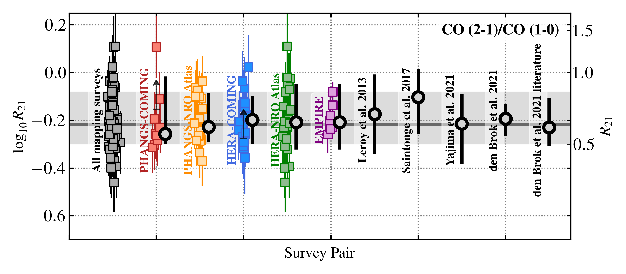
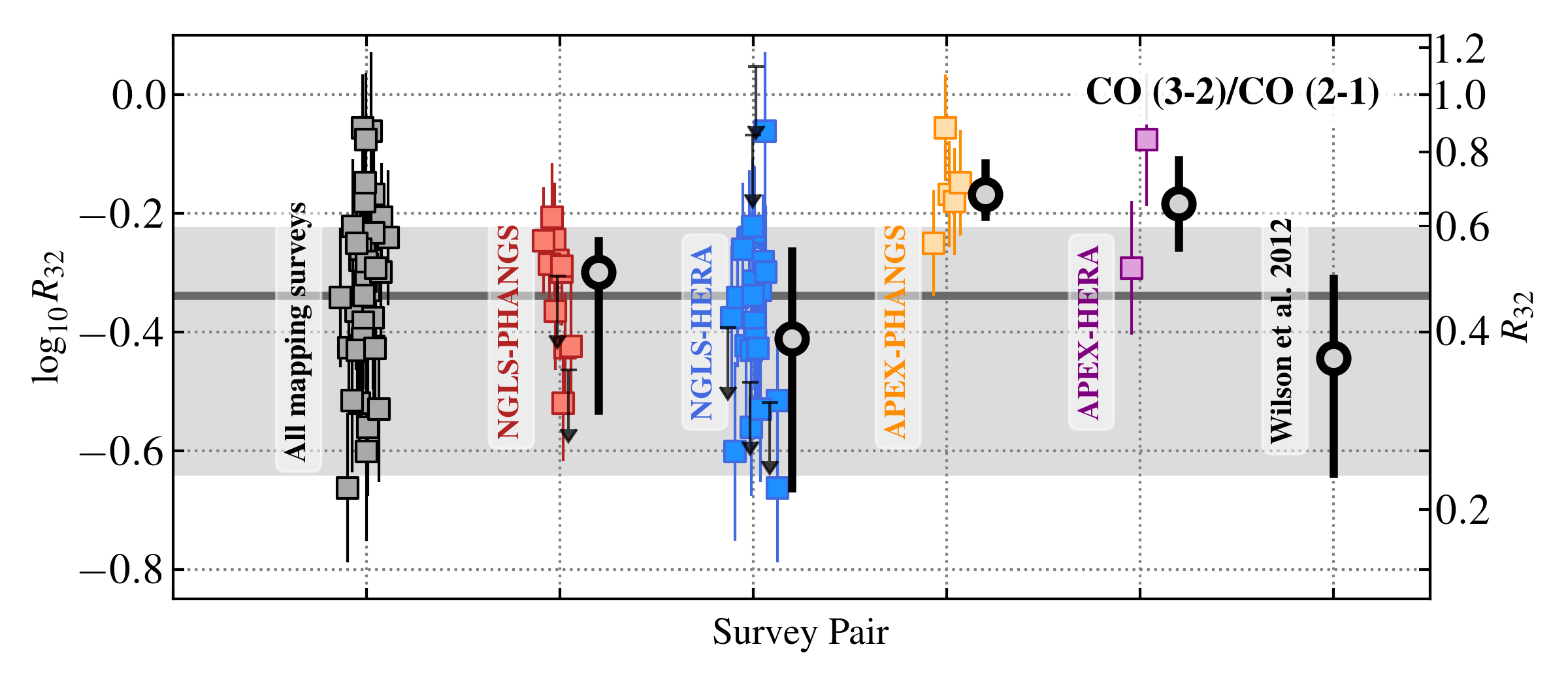
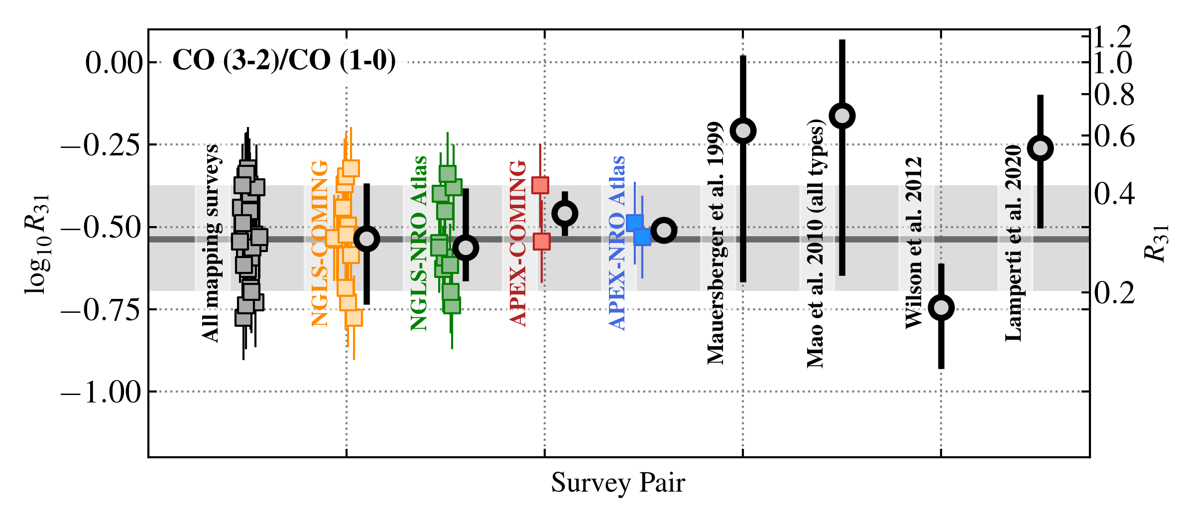
Figure 4: Galaxy-integrated CO line ratios. Colored data points show galaxy-integrated line ratios measured from maps, including limits. The error bars on the individual points reflect both statistical and calibration error as described in §3. For each survey pair or literature result, the black circle shows the median and the error bar shows the $\pm 1\sigma$ reported range for that survey pair or literature study. The top row shows results for $R_{21}$. The middle row shows results for $R_{32}$ and the bottom row shows $R_{31}$. In each panel the thick gray horizontal line and shaded gray region show the median and $16{-}84^{\rm th}$ percentile range from all mapping data (see Table 3) in this study.

In total, as reported in Table 1, we study $152$ pairs of overlapping surveys. For each measured $R_{21}$, $R_{32}$, and $R_{31}$, Table 2 gives the name, survey pair, adopted distance to the galaxy, estimated SFR, $M_{\star}$, and the CO luminosity, $L_{\rm CO}$, in each line. Note that as discussed above, we only quote one CO luminosity per line for each galaxy. This is the $L_{\rm CO}$ that we suggest to use as characteristic of the galaxy, not the value used in the calculation of the line ratio, because our quoted $L_{\rm CO}$ includes an aperture correction. When a galaxy was covered in the same line by multiple surveys, we chose which to use for $L_{\rm CO}$ following the same prioritization of surveys as noted in §3.4.

Figure 4 shows the distribution of the three measured line ratios, along with ranges reported for nearby galaxies in the literature. The first part of each plot shows results for all mapping surveys, then we separate the results according to the survey pair used for the measurement. Table 3 reports basic results for the distributions combining all mapping surveys.

$\bm{R_{21}\equiv\textbf{CO}\,(2{-}1)/\textbf{CO}\,(1{-}0)}$: Treating all data equally, we find a median $R_{21}=0.61$ and a mean $R_{21}=0.65$ with a $16{-}84^{\mathrm{th}}$ percentile range from $0.50{-}0.83$. This reflects $76$ mapping measurements from $43$ galaxies in this work and $9$ measurements from DENBROK21. Note that this distribution allows repeat measurements when the same galaxy was targeted by multiple surveys, and will therefore weigh “popular” targets more heavily. Since our goal here is to synthesize the current literature we consider this approach reasonable, and we use only a single best value for each galaxy when fitting scaling relations below. As Figure 3 shows, the targets of the surveys we consider emphasize high mass, high SFR galaxies (see also §LABEL:sec:biases).

As Figure 4 shows, our $R_{21}$ values agree well with previous results for normal star-forming galaxies. We find an almost identical median value to the $0.64$ measure for EMPIRE galaxies in DENBROK21, though our data show higher scatter than theirs. This likely reflects both the high quality of the EMPIRE CO $(1{\scalebox{0.75}[1.0]{$-$}}0)$ maps presented in DENBROK21 and the narrower range of galaxy properties sampled by EMPIRE, which we illustrate in Figure 3. We also find almost perfect agreement with YAJIMA21, who also derive a median of $R_{21}=0.61$ with a scatter of $\pm 0.19$. The sample in YAJIMA21 represents a subset of our own so we expect this close match. Finally, our measurements also agree reasonably well with previous HERACLES results by LEROY13, who found median $R_{21}$ of $0.67$ with a scatter of $\pm 0.16$ dex or $\pm 44\%$, corresponding to a range of ${\sim}0.46{-}0.97$. Finally, we also agree well with the $0.58$ median and ${\sim}0.49{-}0.77$ $1\sigma$ range for literature single-pointing measurements compiled by DENBROK21.

Our measurements appear slightly lower than the xCOLD GASS measurements by SAINTONGE17. We attribute this mostly to selection effects, though given that the line ratios drop with radius (§LABEL:sec:local) there could also be some mild impact from the limited xCOLD GASS beam size. As Figure 3 shows, the xCOLD GASS $R_{21}$ measurements target a wider range of stellar mass than our current $R_{21}$ sample. The lower mass galaxies and high $\mbox{{SFR}}/M_{\star}$ galaxies in the xCOLD GASS sample likely shift the median to the higher average value of $R_{21}=0.8$ that they report. For reference, if we include the SAINTONGE17 measurements in our sample, the combined data set has median $R_{21}=0.64$, mean $R_{21}=0.74$, and $16{-}84^{\rm th}$ percentile range of $0.52{-}0.91$.

This paper does not focus on individual targets, but we briefly note that the three high $R_{21}>1.0$ values seen in Figure 4 are all consistent with $R_{21}\lesssim 1$ within the uncertainties. These are NGC 1087 in PHANGS–ALMA+COMING, NGC 2976 in HERA+NRO Atlas, and NGC 4536 in HERA+NRO Atlas. Given the sample size and magnitude of the uncertainties, we expect a few such outliers.

Summarizing, Figure 4 shows overall good convergence among recent studies of $R_{21}$. Adopting a typical value of $R_{21}=0.65$ with a $30\%$ uncertainty that reflects scatter across the galaxy population represents a good assumption for high mass, $\log_{10}M_{\star}\,[{\rm M}_{\odot}]\gtrsim 10.25$ (see Figure 3), $z=0$ galaxies on the main sequence of star-forming galaxies (LEROY13; DENBROK21; YAJIMA21).

$\bm{R_{32}\equiv\textbf{CO}\,(3{-}2)/\textbf{CO}\,(2{-}1)}$: We find a median $R_{32}=0.46$ with mean $R_{32}=0.50$ and a $16{-}84^{\rm th}$ percentile range of $0.23{-}0.59$. Because CO $(3{\scalebox{0.75}[1.0]{$-$}}2)$ is comparatively faint and the CO $(2{\scalebox{0.75}[1.0]{$-$}}1)$ data have higher signal-to-noise, upper limits affect our $R_{32}$ distribution more than the other two ratios. We have treated the upper limits as equal to our minimum measured ratio for quantifying the distribution. This choice mainly affects our $16^{\rm th}$ percentile estimate. With $7$ of $40$ $R_{32}$ measurements being upper limits, the $16^{\rm th}$ percentile quoted is set to the lowest measured ratio.

Compared to $R_{21}$ and $R_{31}$, $R_{32}$ has the least extensive sample of previous beam-matched or mapping based studies of whole nearby galaxies; we are only aware of the work by WILSON12, who found mean $R_{32}$ of $0.36$ with $\pm 0.13$ scatter using earlier versions of the same data that we use here. This is moderately lower than our calculated mean value. We attribute part of the difference to revisions to the adopted IRAM main beam efficiency (see above and LEROY13B) after WILSON12 made their measurements, and to our ability to match the areas used for the calculations in this paper, which was not possible in WILSON12. Taking these factors into account, the measurements appear roughly consistent. We also note that in Figure 4 the APEX data and JCMT NGLS data show hints of an offset. As far as we can tell, this reflects a mixture of small number statistics and perhaps the choice to focus the initial APEX LASMA mapping on bright, actively star-forming targets, which may have more excited molecular gas. Only one target overlaps between the two surveys, NGC 3627, and for that case we do find a ${\sim}30\%$ higher CO $(3{\scalebox{0.75}[1.0]{$-$}}2)$ luminosity from APEX than the JCMT, but this is only a single target.

$R_{32}$ does appear to have a larger dynamic range than $R_{21}$. Because lower limits confuse the $16^{\rm th}$ percentile estimate for $R_{32}$, we compare the interquartile ($25{-}75^{\rm th}$ percentile) ranges for the two ratios, and find ${\sim}0.14$ dex range for $R_{21}$ and ${\sim}0.27$ dex for $R_{32}$. Though caveats related to a small sample size and the effect of lower limits still apply, this agrees with the expectation (see §2) that $R_{32}$ shows significant excitation variations across the range of real conditions found in molecular gas and indicates that the ratio has potential to act as a strong diagnostic of local excitation of molecular gas.

$\bm{R_{31}\equiv\textbf{CO}\,(3{-}2)/\textbf{CO}\,(1{-}0)}$: We find a median $R_{31}=0.29$ and a mean $R_{31}=0.30$ with a $16{-}84^{\rm th}$ percentile range of $0.20{-}0.41$. Though the samples used to calculate the ratios vary, our $R_{31}$, $R_{32}$, and $R_{21}$ values approximately “close” as expected with $R_{31}\sim R_{32}\times R_{21}$, implying reasonable self-consistency within our measurements.

The literature reports a wide range of values. Our measurement is high compared to the $0.18\pm 0.06$ reported by WILSON12 comparing NRO Atlas and JCMT NGLS data. Note, however, that WILSON12 caution that they do not match areas for the comparison, so their lower value could simply reflect a mismatch in apertures. Our measurements do agree well with the results for a smaller set of galaxies from WILSON09. They used the NGLS and NRO Atlas to study regions in individual galaxies and found ratios in the ${\sim}0.3{-}0.4$ range.

Our measurements lie on the low end of the range $R_{31}=0.2{-}1.0$ found by MAUERSBERGER99, but note that their sample also includes many starburst and active galaxies and only ${\sim}7$ normal spiral galaxies. A similar case holds for MAO10, who obtained $R_{31}=0.7\pm 0.5$. Partially based on those studies, we expect much higher, approaching thermal, $R_{31}$ in active galaxies and dense galaxies, so the contrast with our more quiescent targets seems reasonable. This appears to be mostly born out by our the results in §4.2. Our values also appear low compared to the mean $R_{31}=0.55$ and $\pm 0.23$ scatter found for $28$ star-forming galaxies by LAMPERTI20 using single-pointing measurements. $R_{31}$ clearly shows a wide dynamic range and so good promise as a diagnostic. However the state of $R_{31}$ observations remains fairly limited, though not quite so much as for $R_{32}$.

With $R_{31}<R_{32}<R_{21}<1$ on average, these values appear consistent with the standard picture that most low-$J$ CO emission from nearby star-forming galaxies comes from optically thick clouds with the CO $(2{\scalebox{0.75}[1.0]{$-$}}1)$ and CO $(3{\scalebox{0.75}[1.0]{$-$}}2)$ transitions moderately sub-thermally excited (e.g., see §2, WEISS05; BOLATTO13B). We discuss this more in Section LABEL:sec:discussion.

4.2 Comparison to integrated galaxy properties

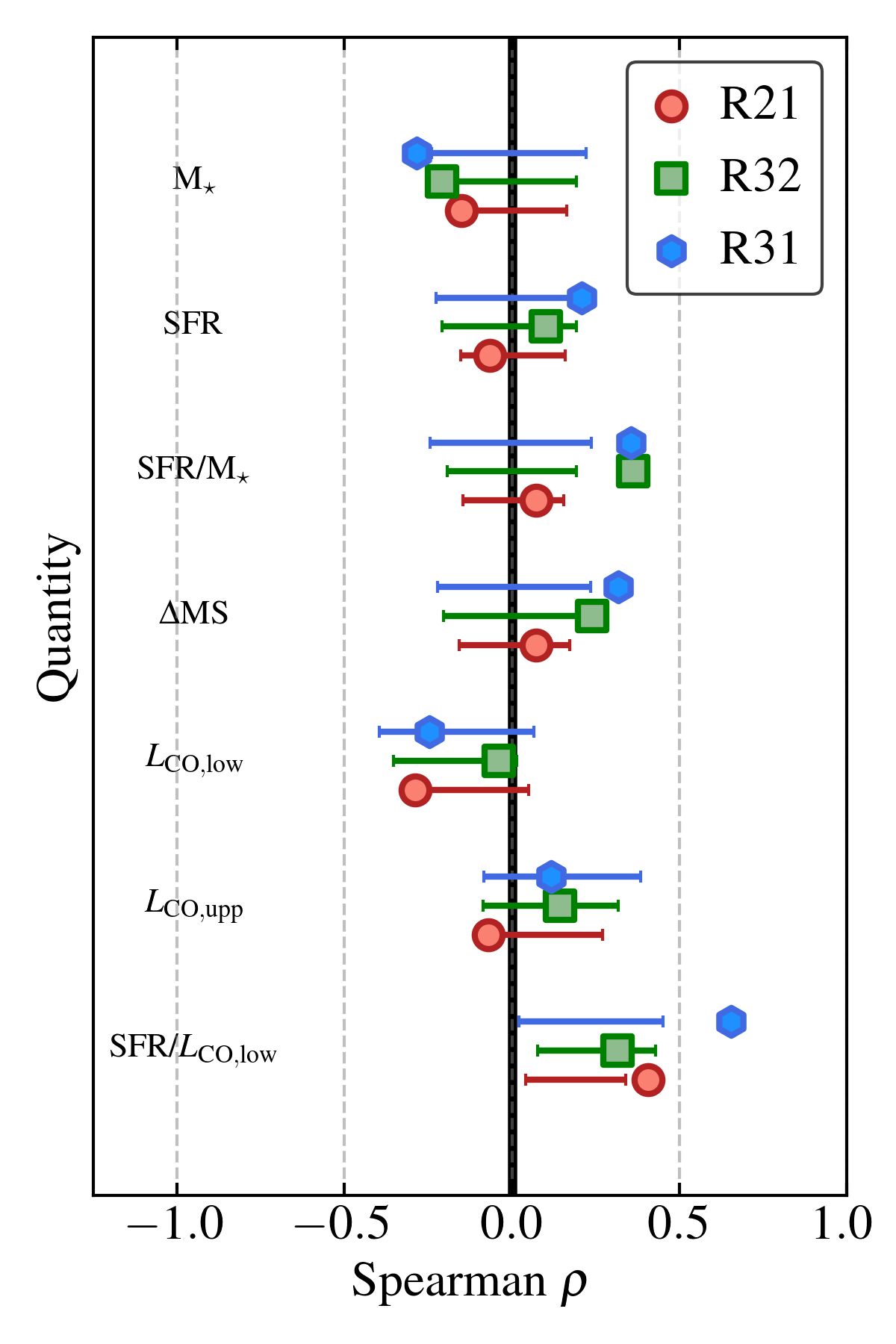
Figure 5: Rank correlation of line ratios with galaxy properties. Spearman rank correlation coefficients relating global galaxy properties to measured line ratios, neglecting limits. The bars show the $16{-}84$% range of coefficients expected under the null hypothesis of no real correlation (N.B., in the cases with correlated axes, the rank correlation coefficient for no true correlation may not be centered on zero, see the text). $L_{\rm CO,low}$ refers to the luminosity of the lower CO transition in the ratio, e.g., CO $(1{\scalebox{0.75}[1.0]{$-$}}0)$ in $R_{21}$, while $L_{\rm CO,upp}$ refers to the upper transition, e.g., CO $(3{\scalebox{0.75}[1.0]{$-$}}2)$ in $R_{31}$. As the contrast between results for $L_{\rm CO,upp}$ and $L_{\rm CO,low}$ demonstrates, the correlated axes play an important but hard-to-avoid role in determining correlations with $L_{\rm CO}$ and $\mbox{{SFR}}/L_{\rm CO}$. Most correlations show marginal significance, but are consistent with low mass, high $\mbox{{SFR}}/M_{\star}$, and high $\mbox{{SFR}}/L_{\rm CO}$ galaxies showing higher line ratios, especially among the measurements involving CO $(3{\scalebox{0.75}[1.0]{$-$}}2)$. See also Figure 6.

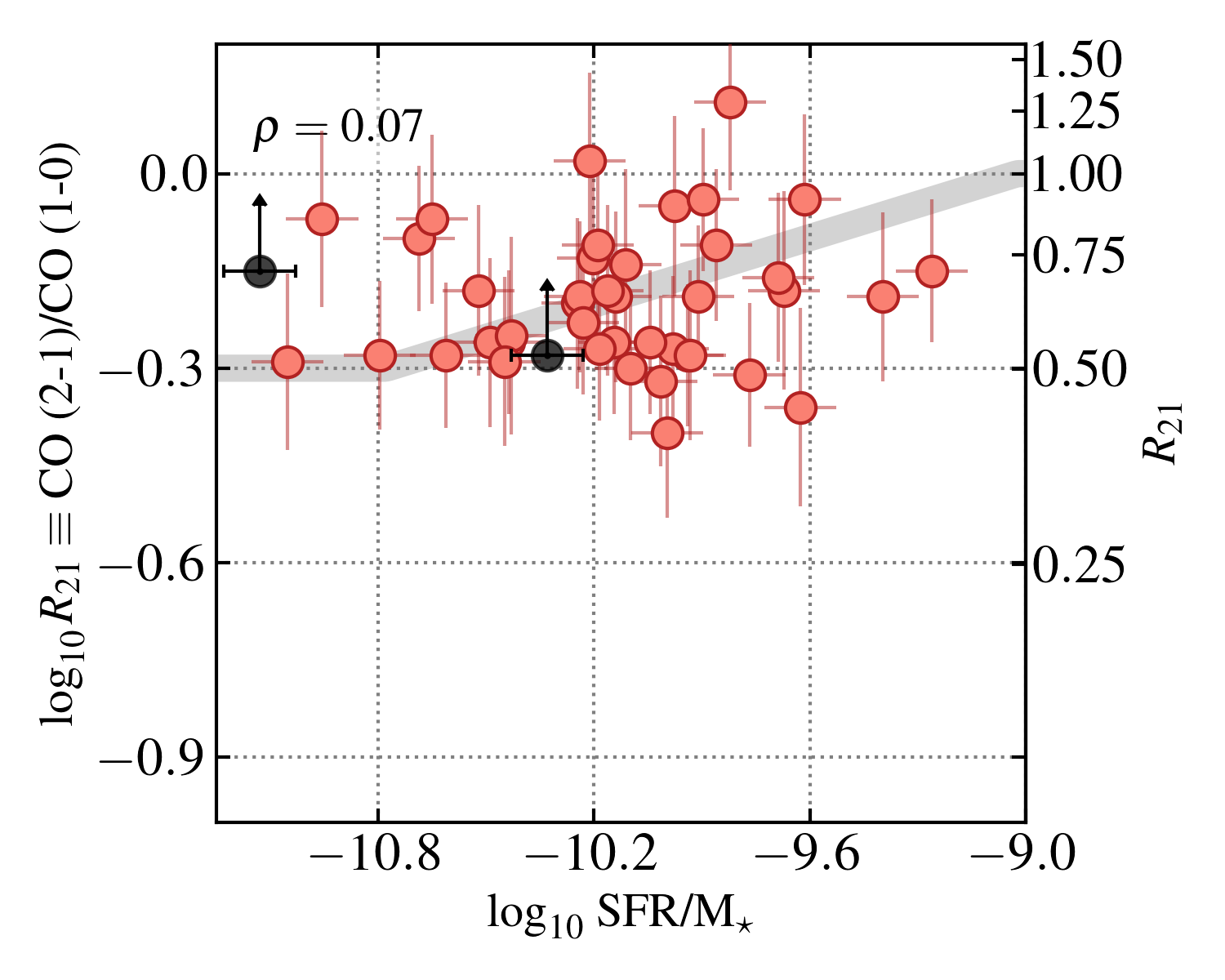
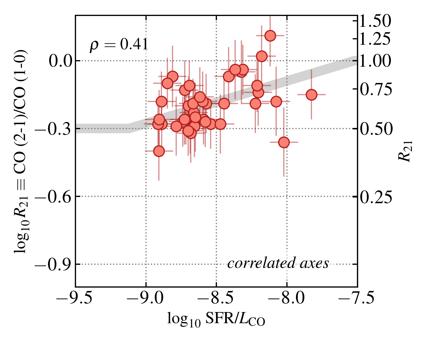
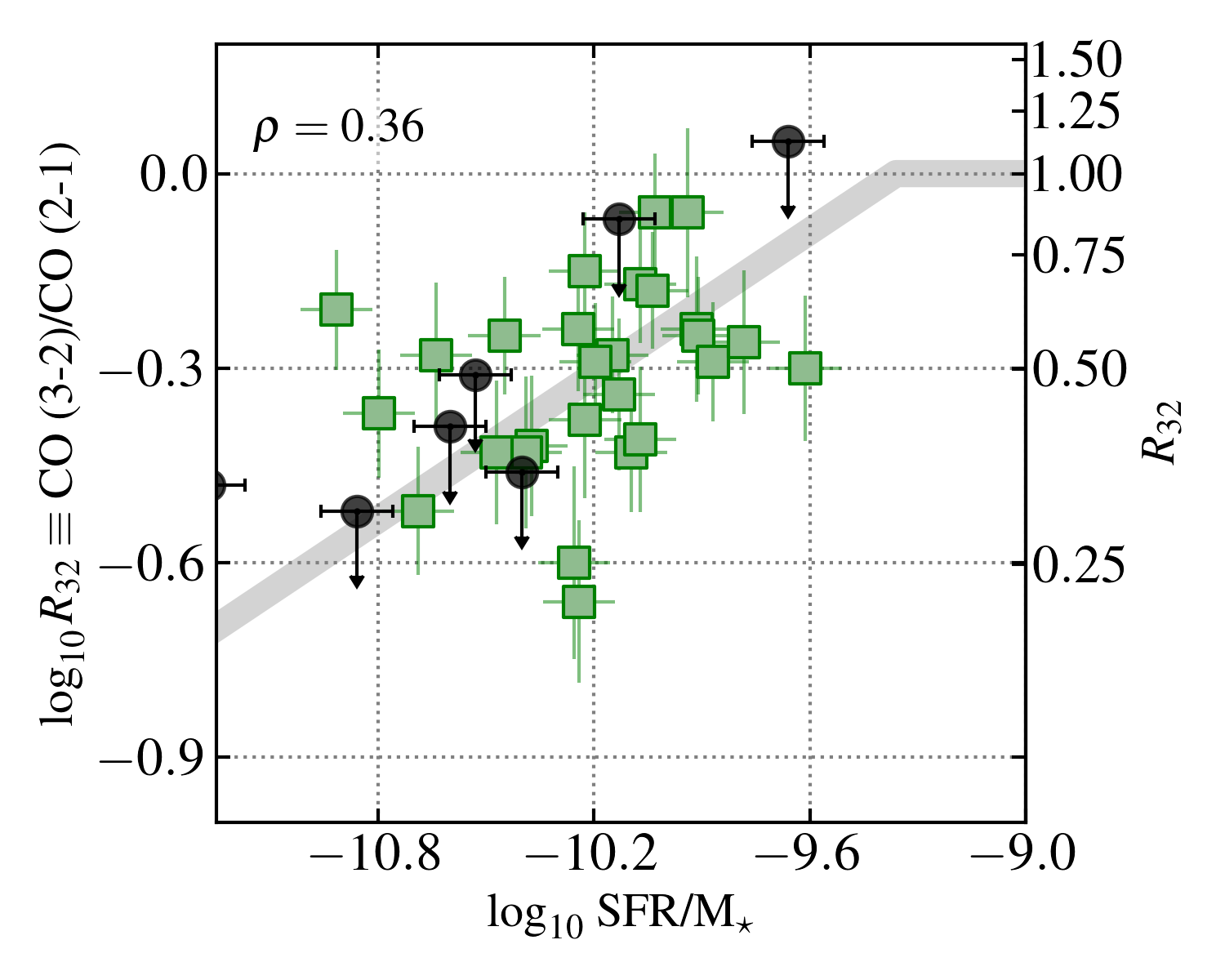
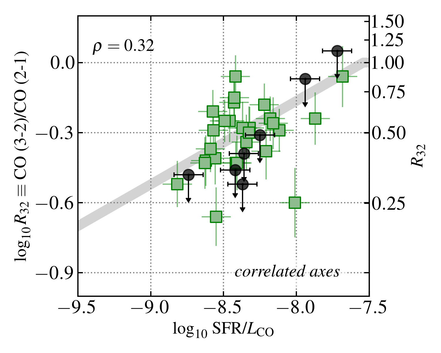
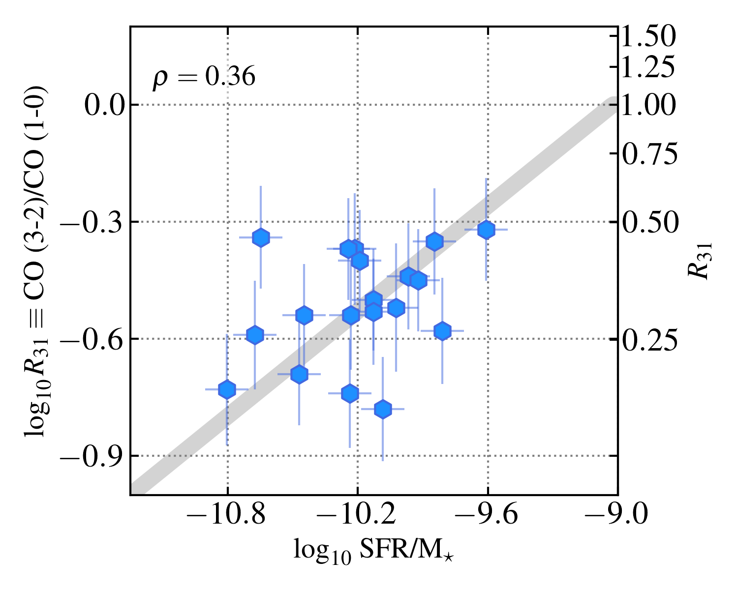
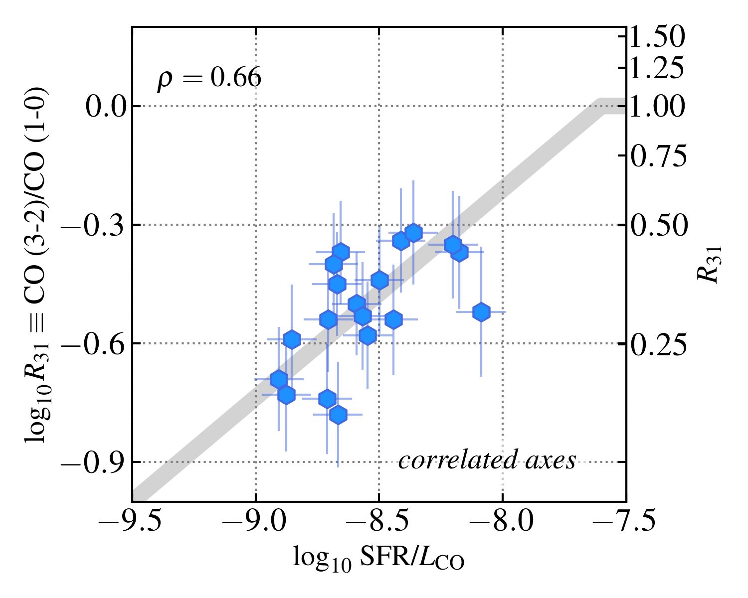
Figure 6: Correlations between line ratios and galaxy-integrated properties. Galaxy-integrated $R_{21}$, $R_{32}$, and $R_{31}$ as function of quantities expected to relate to excitation, specifically $\mbox{{SFR}}/M_{\star}$ and $\mbox{{SFR}}/L_{\rm CO,low}$. Each point represents one map pair for one galaxy, with the black points showing limits. Error bars reflect both statistical and calibration uncertainties. The numbers in the top left corner report the Spearman $\rho$ relating the quantities on the $x$ and $y$ axes. The gray lines show highly approximate scaling relations that go through the data and then saturate at the thermal $\log_{10}R=0$, see §4.2.1, Equation (LABEL:eq:pred_linerat), and Table 4. As discussed in §4.2, the axes in the right hand column are correlated and this may exert a significant effect on the observed relation.

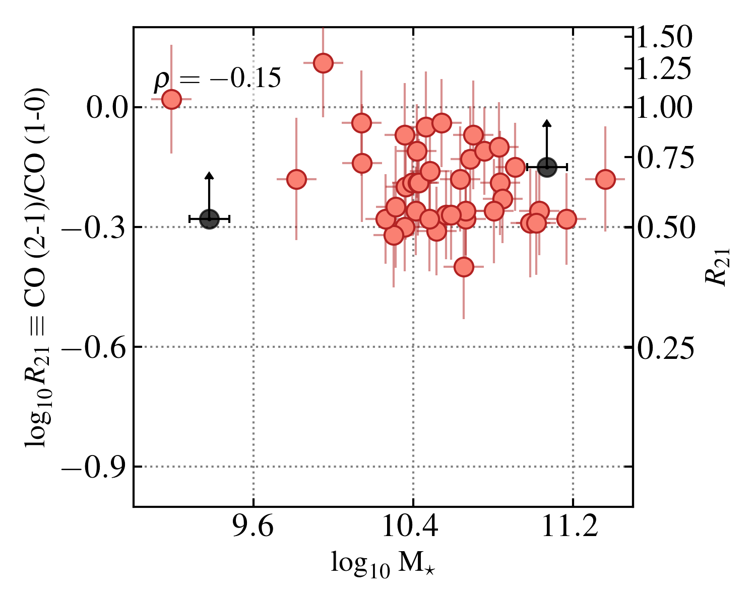
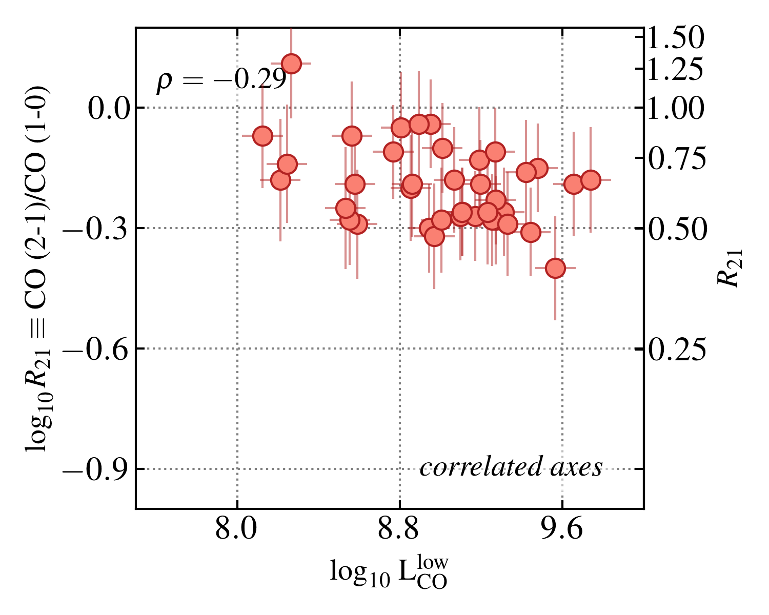
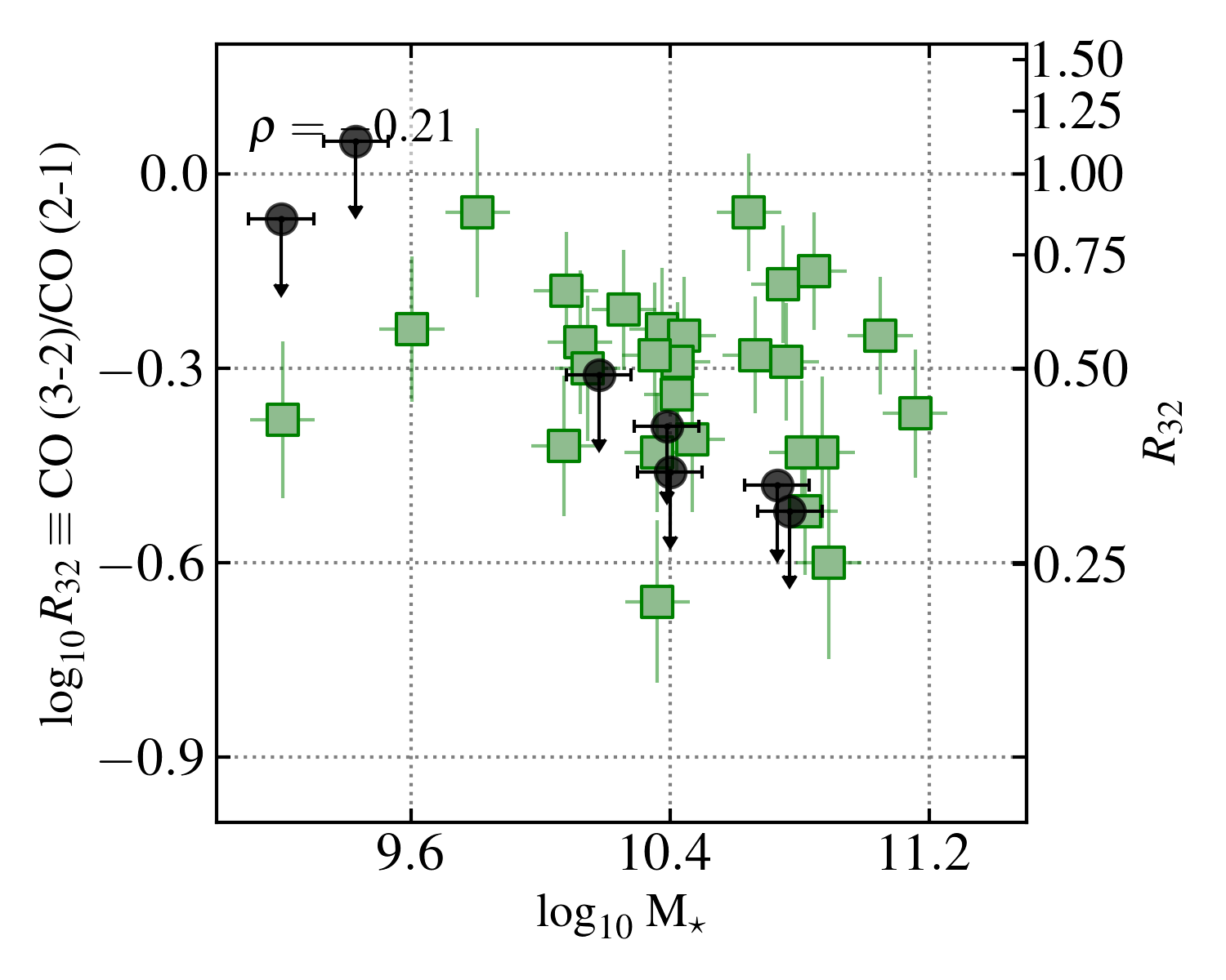
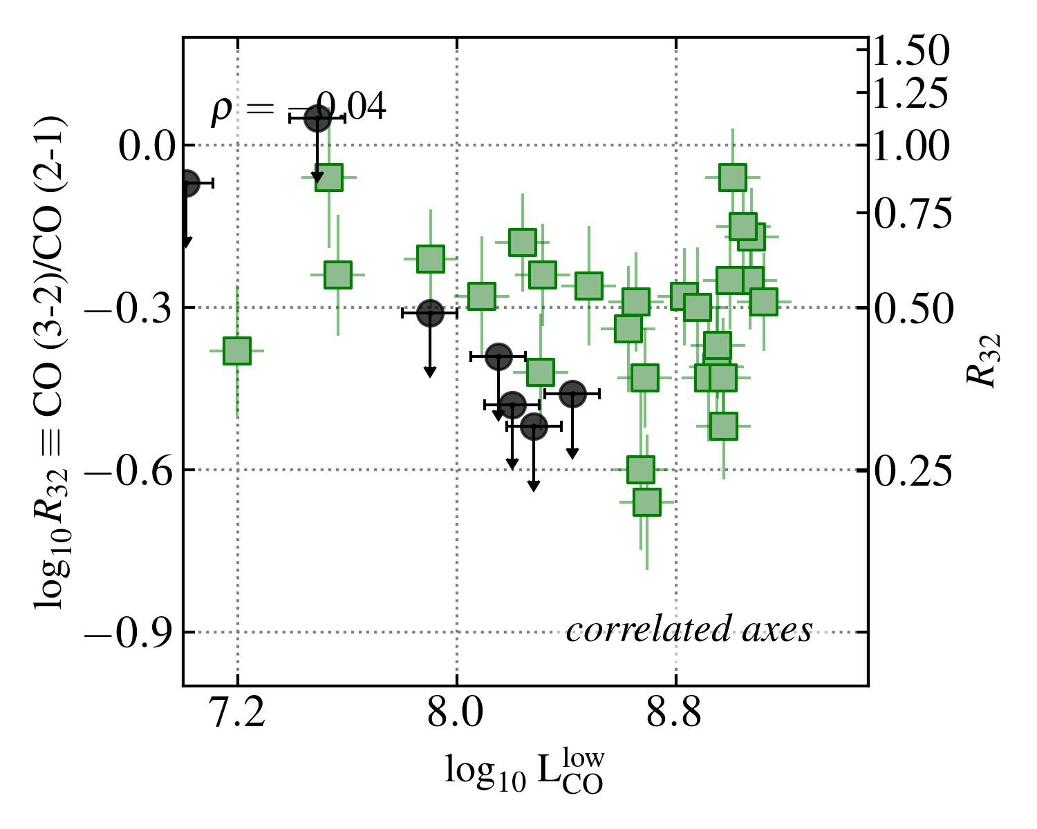
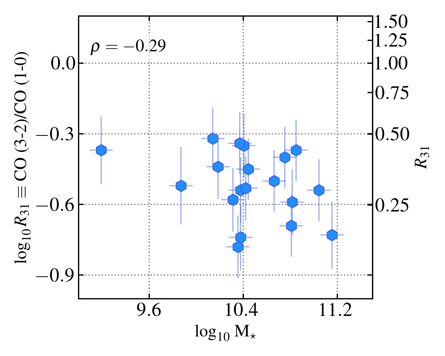
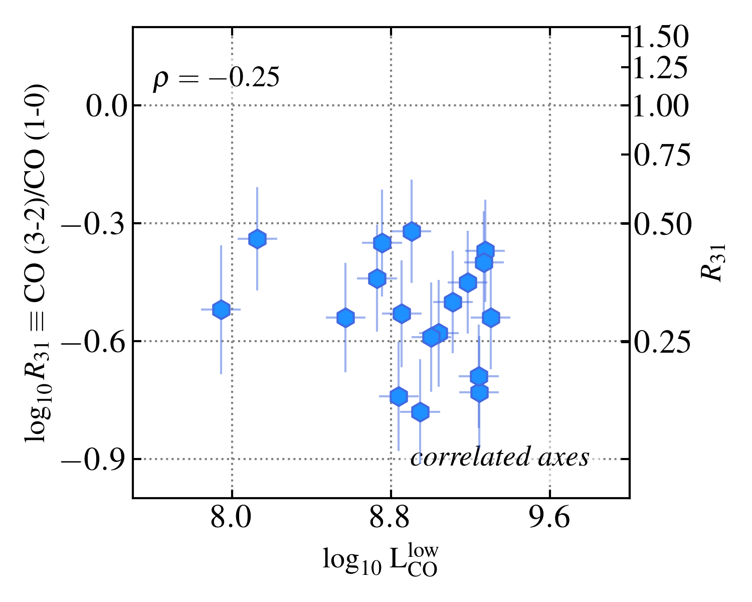
Figure 7: Correlations between line ratios and galaxy-integrated properties. Galaxy-integrated $R_{21}$, $R_{32}$, and $R_{31}$ as function of $M_{\star}$ and $L_{\rm CO,low}$. Each point represents one map pair for one galaxy, with the black points showing limits. Error bars reflect both statistical and calibration uncertainties. The numbers in the top left corner report the Spearman $\rho$ relating the quantities on the $x$ and $y$ axes. As discussed in §4.2, the axes in the right hand column are correlated and this may exert a significant effect on the observed relation. The correlations here appear even weaker than those in Figure 6, and we do not show any possible functional relations.

As discussed in §2, these ratios are both expected and observed to vary between galaxies. We test for correlations between all three line ratios and global galaxy properties in Figures 5 and 6. Before doing so, we again highlight the relatively narrow range of galaxy properties covered by current mapping surveys, visualized in Figure 3 and discussed in §LABEL:sec:biases. Especially for $R_{21}$, the current measurements focus on high-mass galaxies, mostly in the range $\log_{10}M_{\star}\,[{\rm M}_{\odot}]\sim 10.25{-}10.75$ with star formation rates just above the star-forming main sequence. Though the data are sparser for the ratios involving CO $(3{\scalebox{0.75}[1.0]{$-$}}2)$, these measurements do span a larger range of stellar mass and star formation rate at fixed stellar mass.

Figure 5 shows the rank correlation coefficients relating each line ratio to $M_{\star}$, SFR, specific star formation rate ($\mbox{{SFR}}/M_{\star}$), offset from the main sequence of star-forming galaxies ($\Delta{\rm MS}$), CO luminosity, and SFR-per-unit $L_{\rm CO}$ ($\mbox{{SFR}}/L_{\rm CO}$). The colored bars show the expected correlation and $1\sigma$ scatter for the null hypothesis. In the cases of $M_{\star}$, SFR, $\mbox{{SFR}}/M_{\star}$, and $\Delta{\rm MS}$, we adopt the simple null hypothesis that the line ratio and the other variable are not correlated. Then, the expected correlation will be $0$ and the $1\sigma$ scatter reflects the range from randomly re-pairing the variables. Recall that here, unlike in Figure 4, we use only a single best estimate of each line ratio for each galaxy.

In the case of $L_{\rm CO}$ and $\mbox{{SFR}}/L_{\rm CO}$, the two variables used in the correlation will be correlated by construction. In this case, we construct the null hypothesis as follows. First, we measure the logarithmic scatter in the real line ratio across our data set. Then, as the null hypothesis, we assume a fixed underlying line ratio and that this scatter is evenly distributed across the variables involved. We generate the expectations for the null hypothesis by randomly applying this scatter repeatedly to each variable and calculating the rank correlation coefficient. Here, we consider the individual CO luminosities, not the line ratios, as the underlying variables for this exercise. This ensures that the null hypothesis captures the built-in correlation between the axes. For example, when we correlate the line ratio with $L_{\rm CO,upp}$, i.e., the luminosity in the numerator, we measure the scatter in the $\log_{10}$ of the line ratio, $\sigma$, and then we apply $\sqrt{2}$ times $\sigma$ in the model noise to each of $L_{\rm CO,upp}$ and $L_{\rm CO,low}$. Then, we construct the model line ratios $R=L_{\rm CO,upp}/L_{\rm CO,low}$ before calculating the expected correlation. That is, we define the null hypothesis to be the case where the line ratio is fixed and the variance matches the observed variance and is randomly distributed among the relevant variables.

Overall the figure shows a consistent sense of variations. Lower mass galaxies, which also have lower $L_{\rm CO}$, higher $\mbox{{SFR}}/M_{\star}$, and higher $\mbox{{SFR}}/L_{\rm CO}$, tend to show higher line ratios. The absent or weak correlation with SFR can be understood as competing effects: low $M_{\star}$ galaxies have higher $\mbox{{SFR}}/M_{\star}$ but also lower overall SFR. The radiation field in low mass galaxies may be more intense due to a higher local $\Sigma_{\rm SFR}$, but the integrated SFR will still be lower. In general, correlations with integrated galaxy properties appear stronger for $R_{32}$ and $R_{31}$ compared to $R_{21}$. This partially reflects the broader range of galaxy properties covered by those measurements (Figure 3), and may also reflect that $R_{32}$ and $R_{31}$ have more sensitivity than $R_{21}$ to the range of conditions found in normal galaxies (see §2).

These trends make physical sense and agree with the limited previous measurements. Physically, elevated $\mbox{{SFR}}/M_{\star}$ may trace more intense radiation fields and stronger heating of the gas, suggesting higher temperatures. The anticorrelation with $M_{\star}$ may reflect the impact of dust shielding. Based on the existence of the mass–metallicity relation (e.g., TREMONTI04; KEWLEY08), we expect the low mass members of our sample to also have lower dust-to-gas ratios (e.g., LEROY11; REMYRUYER14; CASASOLA19) and more intense radiation fields. In literature studies, CO line ratios do appear enhanced in low metallicity regions or galaxies (e.g., LEQUEUX94; BOLATTO03; DRUARD14; KEPLEY16; CICONE17, among many others). Higher $\mbox{{SFR}}/L_{\rm CO}$ may indicate poorly-shielded, low metallicity gas in which the CO persists only in the core of a molecular cloud (e.g., see discussion in GLOVER12; SCHRUBA12; BOLATTO13A; RUBIO15). Alternatively, higher $\mbox{{SFR}}/L_{\rm CO}$ can indicate more efficiently star-forming gas, which will often be denser gas with more nearby heating sources. These are both factors that can lead to higher line ratios, especially $R_{32}$ and $R_{31}$ (see §2). Given that our sample skews towards relatively massive, and thus nearly solar metallicity targets, we expect that these density and heating effects likely represent the main drivers of the observed correlations. The correlations that we see agree with the results of LAMPERTI20 who showed a correlation between $\mbox{{SFR}}/L_{\rm CO,low}$ and $R_{31}$ and with YAJIMA21, who used a subset of the data we consider here and showed a correlation between $R_{21}$ and $\mbox{{SFR}}/L_{\rm CO,low}$. Qualitatively, Figure 5 echos other results at low and high redshift that show a correlation between normalized star formation activity and excitation (e.g., WEISS05; BOLATTO13A; LIU21).

Although the pattern in Figure 5 makes physical sense, the trends are not particularly significant. The $p$-values relating $M_{\star}$ to $R_{31}$ and $R_{32}$ are only $0.24{-}0.29$. For $\mbox{{SFR}}/M_{\star}$ the $p$-values for $R_{31}$ and $R_{32}$ are ${\sim}0.06{-}0.13$, more significant but still indicating only weak correlations. The other significant correlations involve $L_{\rm CO,low}$, the luminosity of the lower CO transition in the line ratio. We report these because the results make physical sense and are interesting, but the line ratio (${\sim}L_{\rm CO,upp}/L_{\rm CO,low})$, and a quantity involving $L_{\rm CO,low}$ are correlated by construction. To see this, contrast the significant correlations seen in Figure 5 for all line ratios and $L_{\rm CO,low}$ and the lack of similar significant correlations for $L_{\rm CO,upp}$. For the moment, we only caution that these results include the effects of correlated measurements and should be taken as indicative but likely overstate the significance of the correlation in the data.

With these caveats in mind, Figures 6 and 7 visualizes the correlations between each line ratio and global quantities: $\mbox{{SFR}}/M_{\star}$, $\mbox{{SFR}}/L_{\rm CO,low}$, $M_{\star}$, and $L_{\rm CO,low}$. The data show large scatter, but do show evidence for overall correlation with the sense that higher line ratios emerge from galaxies with high $\mbox{{SFR}}/M_{\star}$ and/or $\mbox{{SFR}}/L_{\rm CO}$. The correlations of line ratios with $M_{\star}$ and $L_{\rm CO}^{\rm low}$ appear weaker.

4.2.1 Approximate scaling relations

Table 4: Approximate Scaling Relations

Ratio	Quantity	$y_{\rm low}$	$x_{\rm low}$	$x_{\rm high}$	Scatter
$R_{21}$	$\mbox{{SFR}}/M_{\star}$	$-0.3$	$-10.78$	$-9.02$	$0.07$
$R_{21}$	$\mbox{{SFR}}/L_{\rm CO,low}$	$-0.3$	$-9.12$	$-7.52$	$0.07$
$R_{32}$	$\mbox{{SFR}}/M_{\star}$	$-0.7$	$-11.25$	$-9.36$	$0.10$
$R_{32}$	$\mbox{{SFR}}/L_{\rm CO,low}$	$-0.7$	$-9.50$	$-7.54$	$0.08$
$R_{31}$	$\mbox{{SFR}}/M_{\star}$	$-1.0$	$-11.25$	$-9.02$	$0.08$
$R_{31}$	$\mbox{{SFR}}/L_{\rm CO,low}$	$-1.0$	$-9.50$	$-7.60$	$0.08$

“Scatter” reports the median absolute value of the residuals about the fit in dex.

Note. — Coefficients for the indicative scaling relations following Equation (LABEL:eq:pred_linerat) and illustrated in Figure 6. Fits derived from assuming $y_{\rm low}$ and then fitting $x_{\rm low}$ and $x_{\rm high}$ by minimizing $\chi^{2}$. We report all quantities, including the scatter, in dex. As shown in the figure these should be taken as approximate and we expect future work to revise them considerably.