Theory of superlocalized magnetic nanoparticle hyperthermia:
rotating versus oscillating fields

Abstract

The main idea of magnetic hyperthermia is to increase locally the temperature of the human body by means of injected superparamagnetic nanoparticles. They absorb energy from a time-dependent external magnetic field and transfer it into their environment. In the so-called superlocalization, the combination of an applied oscillating and a static magnetic field gradient provides even more focused heating since for large enough static field the dissipation is considerably reduced. Similar effect was found in the deterministic study of the rotating field combined with a static field gradient. Here we study theoretically the influence of thermal effects on superlocalization and on heating efficiency. We demonstrate that when time-dependent steady state motions of the magnetisation vector are present in the zero temperature limit, then deterministic and stochastic results are very similar to each other. We also show that when steady state motions are absent, the superlocalization is severely reduced by thermal effects. Our most important finding is that in the low frequency range ($\omega\to 0$) suitable for hyperthermia, the oscillating applied field is shown to result in two times larger intrinsic loss power and specific absorption rate then the rotating one with identical superlocalization ability which has importance in technical realisation.

I Introduction

Magnetic nanoparticle hyperthermia pankhurst ; ortega_d ; pankhurst_q_a ; perigo_e_a ; cabrera_d ; clinapp_1 ; clinapp_2 , or magnetic fluid hyperthermia, is an adjuvant cancer therapy where magnetic nanoparticles are injected into the body. The nanoparticles are used to transfer energy from the applied (usually alternating) magnetic field in order to locally increase the temperature, which is used to treat cancer. The idea to use temperature increase of the human body for medical applications has an ancient history. However, the whole-body hyperthermia has limitations since it is very difficult to increase the core temperature of the human body and if we do so it could have serious drawbacks. Thus, one should turn to local heating. The more local the hyperthermia the more effective the treatment is. In general targeted magnetic hyperthermia has a great importance egfr ; domenech_m . Magnetic nanoparticles can be used to achieve a very focused, very well localised heating of the human body. Indeed, there is an increasing interest on how to improve the efficiency of the heat transfer, see e.g., adv_func_mat ; angew_minireview ; review_rinaldi , and also on how to keep the injected particles localised, since they can accumulate in non-targeted tissues non_local_heat . A spatially controlled and image guided nanoscale magnetic hyperthermia have been recently tested in vivo and in vitro experiments mpi_test . This method is based on a combination of an applied alternating and a static field gradient which provides a spatially focused heating focused_hyperthermia_1 ; focused_hyperthermia_2 ; focused_hyperthermia_3 ; focused_hyperthermia_4 ; recent_focused_hyperthermia . The reason is that for large enough static field the dissipation drops to zero, and therefore the temperature increase is observed mostly where the static field vanishes. This is an instance of the phenomenon referred to as ”superlocalization”, i.e., the controllable localization of the temperature increase by the usage of combinations of inhomogeneous static and time-dependent magnetic fields. This can also be understood by considering the area of the dynamic hysteresis loops. For oscillating applied field, the area of the dynamic hysteresis loops becomes narrow if the static field is present, thus, the amount of energy transferred is decreased and one expects a bell-shaped curve of the energy transfer as a function of the static field amplitude, see, e.g., Fig. (10.4) of review_rinaldi or for more details MRSh_theory_focused . The idea of spatially focused, i.e., superlocalized selective heating of a desired region provides us a very precise heating mechanism which is realised in recent in vivo experiments mpi_test .

A recent proposal stat_rot_fields discusses the possibility of a superlocalized and enhanced magnetic hyperthermia by an appropriately chosen combination of static and rotating applied fields where the amplitudes of the (in-plane) static and rotating fields fulfil a certain relation. For example, in case of magnetically isotropic nanoparticles the amplitudes of the applied magnetic field (static and rotating) should be the same. The advantage of the method presented in stat_rot_fields is the drastic enhancement of the heat transfer which can be very well localised by a static field gradient, i.e.,spatially controlled by the ratio of the amplitudes of the static and rotating applied fields. Another recent example is Ref. kim , where the dynamics and the energy dissipation in the presence of a static and rotating fields have been studied and enhancement effects are reported, however the frequency range is too large to be applicable for hyperthermia. Indeed, the applied external magnetic field is one of the most easily variable parameters to increase the efficiency of heat generation and one finds several attempts in the literature where the case of the rotating external magnetic field has been studied, as an example see the selection Bertotti ; Denisov_1 ; Denisov_2 ; Cantillon ; Ahsen ; Raikher_Stephanov ; Denisov_thermal ; Denisov_thermal_1 ; Lyutyy ; Lyutyy_energy ; Chen ; exp_rot ; lyutyy_general ; viscous_rotating .

If the applied frequency is high enough ($\omega\gtrsim 100$ kHz) and the diameter of the nanoparticle is appropriately chosen (typically small enough), the mechanical rotation of the nanoparticles in the surrounding medium is restricted and one can estimate the efficiency of the heat transfer by considering the change in the orientation of the magnetization vector, which is called the Neel relaxation process, lyutyy_general ; neel_brown ; viscous_rotating ; hergt_dutz_2 . On the other hand the applied frequency and the product of the frequency and field amplitude cannot be arbitrarily large due to the biological limitation of hyperthermic treatment of the human body hergt_dutz_1 ; hergt_dutz_2 ; hergt_dutz_3 . On the one hand, in order to minimise eddy currents, the limiting threshold for frequencies is beyond several hundred kHz (certainly not more than 1000 kHz). On the other hand, the product (of the frequency and field strength) is related to the power injected, so, it has to be smaller then an upper bound, the so called Hergt-Dutz limit hergt_dutz_1 ; hergt_dutz_2 ; hergt_dutz_3 . General advice is to use a field frequency of several hundred kHz in combination with rather low field amplitude (few kA/m) or a relatively high field amplitude (a few tens of kA/m) in combination with a frequency of a few hundred kHz. Therefore, if the applied frequency and the applied field amplitude are chosen appropriately, it can be used for hyperthermia and in addition the energy loss depends on the dynamics of the magnetization only, which can be described by the so called Landau-Lifshitz-Gilbert (LLG) equation LLG_1 ; LLG_2 . Let us note that a different theoretical approach to study the relaxation and obtain the dynamic hysteresis loop is the use of the so called Martensyuk, Raikher, and Shliomis (MRSh) equation, which has been applied to consider the focused (superlocalized) hyperthermia in MRSh_theory_focused . The MRSh equation stands for the average magnetisation but the LLG equation describes the dynamics of a single magnetic moment which is used to calculate the time-dependence of the average moment. In this work we rely on the LLG approach.

In view of experimental realisations, it is crucial to consider the influence of thermal fluctuations. Such effects were not taken into account in study of the dynamics of the magnetization performed using the deterministic LLG equation, such as in stat_rot_fields . The effect of thermal fluctuations can be studied by using the stochastic LLG approach sLLG_1 ; sLLG_2 . The motivation of the present work is to explore how thermal fluctuations can affect the superlocalization in presence of static and alternating (oscillating or rotating) fields. Thus, our main goal here is to investigate the influence of thermal effects by means of the stochastic LLG equation on superlocalization and heating efficiency, and to compare the rotating and oscillating cases in the presence of a static magnetic field.

Although, we show that the combination of static and rotating fields can have importance in the technical realisation of magnetic nanoparticle hyperthermia, we put serious limitations on the heating efficiency of the rotating applied field compared to the usual oscillating one.

II Deterministic and stochastic LLG equations

In the following, we use various types of approximations which simplifies the treatment and allow for to get qualitative results on the dependence of the heat transfer on the parameters of the magnetic fields. First, we shall consider individual nanoparticles with a single magnetic domain, so we do not take into account the possible aggregation of these isolated particles, which usually decreases the efficiency of the heat transfer. As mentioned above, only the change of the orientation of the magnetic moments are considered and we neglect the effects coming from the rotation of the particle as a whole which is a suitable approximation if the applied frequency is high and the diameter of the particles is small enough. We do not study the dependence of our results on the size of the nanoparticles. Therefore, we use a typical choice for their diameter which is $\sim 20$ nm, see below for more comments on this point. Finally, we assume magnetically isotropic nanoparticles.

As discussed in the introduction, we use here the LLG equation to determine the motion of the magnetic moment of a single nanoparticle. The Gilbert-form of the deterministic LLG equation reads

$$\frac{\rm{d}}{\rm{d}t}{\bf M}=-\mu_{0}\gamma_{0}{\bf M}\times\left[{\bf H}_{{\mathrm{eff}}}-\eta\frac{\rm{d}}{\rm{d}t}{\bf M}\right],$$ (1)

with the unit vector ${\bf M}={\bf m}/m_{S}$, where m stands for the magnetization vector of a single-domain particle normalised by the saturation magnetic moment $m_{S}$ (e.g., $m_{S}\approx 10^{5}$ A/m for a single crystal Fe₃O₄ Fannin ). Moreover, $\gamma_{0}=1.76\times 10^{11}$ Am²/Js is the gyromagnetic ratio, $\mu_{0}=4\pi\times 10^{-7}$ Tm/A (or N/A²) is the permeability of free space, $\eta$ is the damping factor and finally ${\bf H}_{{\mathrm{eff}}}$ is the local effective magnetic field. The LLG equation retains the magnitude of the magnetization (this is why one can introduce a unit vector for the magnetization) and only the orientation changes in time. It is therefore convenient to use polar coordinates.

Following the notation of Refs. aniso ; Chatel ; heat_enhance ; stat_rot_fields , the Gilbert-form (1) can be equivalently rewritten as

$$\frac{\rm{d}}{\rm{d}t}{\bf M}=-\gamma^{\prime}[{\bf M\times H_{\rm{eff}}}]+\alpha^{\prime}[[{\bf M\times H_{\rm{eff}}]\times M}],$$ (2)

which is the LLG equation where $\gamma^{\prime}=\mu_{0}\gamma_{0}/(1+\alpha^{2})$, $\alpha^{\prime}=\gamma^{\prime}\alpha$ with the dimensionless damping $\alpha=\mu_{0}\gamma_{0}\eta$. Typical values for the damping parameter $\alpha$ are $\alpha=0.1$ and $\alpha=0.3$, which have been used in Lyutyy_energy and Giordano , respectively. In this paper we use $\alpha=0.05$, $\alpha=0.1$ and $\alpha=0.3$.

The local effective magnetic field contains the external applied and the anisotropy fields. As mentioned above, we consider only spherically symmetric nanoparticles without any crystal field anisotropy so, the nanoparticles are considered as isotropic. Several different type of external applied fields combination of static and alternating terms can be considered. The latter can be either oscillating or rotating:

$${\mathrm{Rotating:}}\hskip 14.22636pt{\bf H}_{\rm{eff}}=H\,\,\Big{(}\cos(\omega t)+b_{0},\,\,\sin(\omega t),\,\,0\Big{)},$$ (3)

$${\mathrm{Parallel\,\,oscillating:}}\hskip 14.22636pt{\bf H}_{\rm{eff}}=H\,\,\Big{(}\cos(\omega t)+b_{0},\,\,0,\,\,0\Big{)},$$ (4)

$${\mathrm{Perpendicular\,\,oscillating:}}\hskip 14.22636pt{\bf H}_{\rm{eff}}=H\,\,\Big{(}\cos(\omega t),\,\,b_{0},\,\,0\Big{)},$$ (5)

where $H$ and $Hb_{0}$ stands for the amplitude of the applied and the static fields, respectively.

The heat transfer is a monotonic increasing function of the product of the applied frequency and the field amplitude but at the same time one cannot increase them too much, otherwise they would not usable for medical applications hergt_dutz_1 ; hergt_dutz_2 ; hergt_dutz_3 . For example, the heating efficiency of magnetic nanoparticles was considered for relatively high amplitudes $100$ kA/m at $150$ kHz in high_amplitude . The upper bound on the product of amplitude and frequency is the Hergt-Dutz limit and the value $5\times 10^{8}$ A/(m s) is used as a safe operational guideline review_rinaldi . In other experimental studies it was found that this upper limit might be exceeded by a factor of 10. Indeed, an example for clinical application, one should mention the human-sized magnetic field applicator (developed by MagForce Nanotechnologies AG Berlin, Germany) which can generate a $100$ kHz alternating magnetic field at a variable field strength of $0-18$ kA/m, magforce_1 ; magforce_2 which results in $2\times 10^{9}$ A/(m s) as an upper limit. To explore the dependence on other parameters it is therefore reasonable to keep the product of the frequency and the field amplitude as large as possible. Thus, in this work our choice for the upper (theoretical) limit is $\omega\approx 1000$ kHz and $H\approx 18$kA/m although it is above the safe operational limit. Of course, the Hergt-Dutz limit allow us to use different values for $\omega$ and $H$ but always keeping their product below its maximum value and in addition keeping the frequency below its maximum which is $\omega\approx 1000$ kHz. In this work we fix $H=18$ kA/m but in the very last section where we perform a systematic search for the optimal choice for $\omega$ and $H$ both for the oscillating and the rotating cases. We define as well the parameters

$$\omega_{L} = H\gamma^{\prime}$$

$$\alpha_{N} = H\alpha^{\prime}.$$ (6)

Thus, if one takes $\alpha=0.1$ (and $H=18$ kA/m), a good and typical choice for parameters suitable for hyperthermia is $\omega_{L}=4\times 10^{9}\,{\mathrm{Hz}}$ and $\alpha_{N}=4\times 10^{8}\,{\mathrm{Hz}}$. One can introduce the dimensionless parameters

$$\omega \to \omega t_{0}$$

$$\omega_{L}=H\gamma^{\prime} \to \omega_{L}t_{0}$$

$$\alpha_{N}=H\alpha^{\prime} \to \alpha_{N}t_{0}.$$ (7)

where the dimension has been rescaled by a suitably chosen time parameter $t_{0}$. Here we use $t_{0}=0.5\times 10^{-10}$s. In summary, we use the following sets of dimensionless parameters:

$$\alpha=0.05\,\Rightarrow\,\omega_{L}\sim 0.2,\,\,\,\alpha_{N}\sim 0.01,$$

$$\alpha=0.1\,\Rightarrow\,\omega_{L}\sim 0.2,\,\,\,\alpha_{N}\sim 0.02,$$

$$\alpha=0.3\,\Rightarrow\,\omega_{L}\sim 0.2,\,\,\,\alpha_{N}\sim 0.06.$$ (8)

For hyperthermia one has to take the low-frequency limit, so, a realistic choice for the dimensionless frequency is $\omega\sim 10^{-4}$ which corresponds to the dimensionful value $\sim 2\times 10^{6}$ Hz.

As a next step we introduce the stochastic LLG equation sLLG_1 ; sLLG_2 where thermal fluctuations are taken into account by introducing a random magnetic field, ${\bf H}$, in Eq. (1):

$$\frac{\rm{d}}{\rm{d}t}{\bf M}=-\mu_{0}\gamma_{0}{\bf M}\times\left[({\bf H}_{{\mathrm{eff}}}+{\bf H})-\eta\frac{\rm{d}}{\rm{d}t}{\bf M}\right].$$ (9)

The corresponding stochastic form of the deterministic LLG equation (2) can be written as

$$\frac{\rm{d}}{\rm{d}t}{\bf M}=-\gamma^{\prime}[{\bf M\times(H_{\rm{eff}}+H)}]+\alpha^{\prime}[[{\bf M\times(H_{\rm{eff}}+H)]\times M}],$$ (10)

where the stochastic field, ${\bf H}=(H_{x},H_{y},H_{z})$, consists of Cartesian components which are independent Gaussian white noise variables with the following properties,

$$\langle H_{i}(t)\rangle=0,\hskip 14.22636pt\langle H_{i}(t_{1})H_{j}(t_{2})\rangle=2\,D\,\delta_{ij}\,\delta(t_{1}-t_{2})$$ (11)

where $i=x,y,z$ and $D$ is a parameter defined using the fluctuation-dissipation theorem as $D=\eta k_{B}T/(m_{s}V\mu_{0})$ with the Boltzmann factor $k_{B}$, absolute temperature $T$ and the volume of the particle $V$, see e.g., path_int_sllg . Let us draw the attention of the reader to the dependence of the stochastic description on the volume of the particles. We do not investigate in particular the dependence of our results on the diameter of the individual particles, but the volume cannot be too small since then the nanoparticles will not stored in the human body a long enough time and, at the same time it cannot be too large because then particles have multiple magnetic domains which is not favourable regarding the heating efficiency. A typical choice for the diameter is around $20-50$ nm and we adopt the size $20$nm in this work.

In Eq. (11) the angular brackets stand for averaging over all possible realisations of the stochastic field ${\bf H}(t)$. Due to the Gaussian white noise nature of the stochastic field, the random process of ${\bf M}(t)$ is a Markovian one. So, one can use the Fokker-Planck formalism. We observe that it is known that in the semi-classical limit the Keldysh functional approach reduces to the Fokker-Planck equation. The general path integral approach in the framework of effective field theories using renormalization group techniques is still an active research field, see e.g., ctp_rg ; ctp_rg_1 .

The stochastic LLG equation (10) can be reduced to (or equivalently rewritten as) a system of two stochastic differential equations for the polar $\theta$ and azimuthal $\phi$ angles, see Refs. Giordano ; Denisov_thermal ; Denisov_thermal_1 . In a spherical coordinate system the effect of the thermal bath appears as a Brownian motion on a sphere, which can be described by the Ito process

$$\frac{\rm{d}}{\rm{d}t}\phi =\frac{1}{\sin\theta}\sqrt{\frac{1}{2\tau_{N}}}n_{\phi},$$ (12)

$$\frac{\rm{d}}{\rm{d}t}\theta =\frac{1}{2\tau_{N}}\frac{\cos\theta}{\sin\theta}+\sqrt{\frac{1}{2\tau_{N}}}n_{\theta}.$$ (13)

Here $\tau_{N}\propto 1/T$ is the Néel time for which we used the value $\tau_{N}=1.5\times 10^{-7}s$ at $T=300$K. The role of the random white noise is played by the Gaussian variables $n_{\phi}$ and $n_{\theta}$, which satisfy the standard properties

$$\langle n_{\phi}(t)\rangle=\langle n_{\theta}(t)\rangle=\langle n_{\phi}(t_{1})n_{\theta}(t_{2})\rangle=0,\hskip 28.45274pt\langle n_{\phi}(t_{1})n_{\phi}(t_{2})\rangle=2\,\delta(t_{1}-t_{2}),\;\;\;\langle n_{\theta}(t_{1})n_{\theta}(t_{2})\rangle=2\,\delta(t_{1}-t_{2}).$$ (14)

Of course these equations are only valid without external fields, however the rhs. of Eqs. (12) (13) represents the only difference between the stochastic and deterministic LLG equation. In $T\to 0$ these terms vanish and the stochastic LLG equation reduces to the deterministic one. We developed codes to solve numerically the stochastic differential equations in the presence of a static and rotating applied field defined by Eqs. (3), (4) and (5). The codes are written in python and Mathematica wolfram where the built-in functions for Ito processes are used. Consistency checks and a specific exapmle are shown in Appendix A. In the more complicated cases below, the procedure is the same, the stochastic LLG equations are solved in the same manner in the spherical coordinate system, however the equations are lengthy without containing meaningful new information and thus they are not written.

The energy loss in a single cycle can be easily obtained if the solution $\bf M$ of the LLG equation is known:

$$E=\mu_{0}m_{S}\int_{0}^{\frac{2\pi}{\omega}}{\mathrm{d}}t\left({\bf H}_{\rm{eff}}\cdot\frac{d{\bf M}}{dt}\right).$$ (15)

Two important notes are in order, (i) the above formula contains the average magnetisation $\bf M$, (ii) it holds for a single particle more precisely it has a dimension of J/m³.

The formula (15) gives exactly the same result as the area of the dynamic hysteresis loop which we discuss later. Moreover, the energy loss obtained by either the area of the dynamical hysteresis loop or by the energy loss formula (15) is related to the imaginary part of the frequency-dependent susceptibility. The product of the applied frequency $f$ and the energy $E$ obtained in a single cycle (15) for a single particle and is related to the amount of energy absorbed in a second, i.e, the specific absorption rate (SAR),

$$Ef\propto{\mathrm{SAR}}=\frac{\Delta T\,\,c}{t}$$ (16)

where $\Delta T$ is the temperature increment, $c$ the specific heat and $t$ is the time of the heating period. Notice that the SAR is sometimes referred to as the specific loss power. Furthermore, it is useful to define the so called intrinsic loss power (ILP) ilp ,

$${\mathrm{ILP}}=\frac{{\mathrm{SAR}}}{H^{2}f}$$ (17)

which can be used to compare experimental (and theoretical) SAR values determined at different magnetic field frequencies $f$ and/or amplitudes $H$. Thus, from equation (15) we have

$$\frac{E}{2\pi\mu_{0}m_{s}H^{2}}\propto{\mathrm{ILP}}.$$ (18)

III Non-stochastic limit

We consider in this section the non-stochastic, deterministic, zero temperature limit of the stochastic LLG. A feature of the non-stochastic limit, provided by the deterministic LLG (2) is that the steady state solutions equation can be obtained. These steady state solutions (if they exist) are attractive ones, meaning that, independently of the initial conditions for the magnetization vector, the solution of the LLG equation tends to these steady state ones. Consequently the energy loss can be calculated by simply inserting the steady state solutions into the energy loss formula (15). In this section we discuss these steady state solutions for the oscillating and rotating cases defined by Eqs. (3), (4), (5).

III.1 Rotating case

In this subsection we study the energy losses for the LLG without thermal fluctuations in the rotating case:

$${\bf H}_{\rm{eff}}=H\,\,\Big{(}\cos(\omega t)+b_{0},\,\,\sin(\omega t),\,\,0\Big{)}.$$ (19)

If the static field is in the plane of rotation, the time-dependent magnetization tends to a steady state motion which is a limit-cycle in the reference frame attached to the rotating field, see Fig. 1.

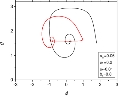
Figure 1: (Color online.) Limit-cycle (red line) of the orbit map in polar coordinates in the rotating frame for isotropic nanoparticles when static field is assumed to be in the plane of rotation. This result is obtained by the deterministic LLG equation, i.e., at zero temperature stat_rot_fields , with the following dimensionless parameters: $\alpha_{N}=0.06$, $\omega_{L}=0.2$, $\omega=0.01$, and $b_{0}=0.8$.

If the static field is perpendicular to the plane of rotation or if it vanishes, the steady state solution of the LLG equation (2) is a fixed point in the rotating frame. Therefore, instead of red coloured limit cycle of Fig. 2 one finds fixed points, see e.g., aniso ; Chatel ; heat_enhance ; stat_rot_fields . It is, however, always true that the steady state solutions are attractive ones which means that the magnetization converges very rapidly to these solutions which can be used to determine the heat transfer.

If the amplitude of the static and rotating fields are identical, the energy loss obtained by the steady state solution of the deterministic LLG equation has a maximum, i.e., for $|b_{0}|=1$ one finds peaks in Fig. 2.

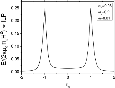
Figure 2: Normalised energy loss (15) is plotted against the parameter $b_{0}$ based on the solution of the deterministic LLG equation (2), with parameters $\alpha_{N}=0.06$, $\omega_{L}=0.2$ and $\omega=0.01$.

The peaks of Fig. 2 clearly show that one finds a drastic enhancement of the energy loss for $|b_{0}|=1$. In addition, if a static field gradient has been used than the heat transfer is not just increased, but also superlocalized since in this case tissues are heated up significantly only where the amplitudes of the static and rotating fields are the same.

Since this result is obtained in the framework of the deterministic LLG equation (2), for experimental realisation one has to take into account thermal fluctuations – which can be done by using the stochastic version of the LLG approach – to see whether the superlocalization is spoiled or not by temperature effects.

III.2 Vanishing static field, oscillating case

Let consider a vanishing static field, i.e., when only oscillating field is applied:

$${\bf H}_{\rm{eff}}=H\,\,\Big{(}\cos(\omega t),\,\,0,\,\,0\Big{)}.$$ (20)

In this case the solution of the deterministic LLG equation (2) can be obtained analytically Chatel :

$$M_{x}(t) = \frac{(M_{x0}-1)+(M_{x0}+1)\exp{\left[\frac{2\alpha_{N}}{\omega}\sin(\omega t)\right]}}{(1-M_{x0})+(M_{x0}+1)\exp{\left[\frac{2\alpha_{N}}{\omega}\sin(\omega t)\right]}},$$

$$M_{y}(t) = \sqrt{1-M_{x}^{2}(t)}\,\,\sin\left[\frac{\omega_{L}}{\omega}\sin(\omega t)+\delta_{0}\right],$$

$$M_{z}(t) = \sqrt{1-M_{x}^{2}(t)}\,\,\cos\left[\frac{\omega_{L}}{\omega}\sin(\omega t)+\delta_{0}\right],$$ (21)

with the parameters $M_{x0}$ and $\delta_{0}$ determined by the initial values $M_{x0}=M_{x}(0)$ and $\delta_{0}=\tan^{-1}(M_{y}(0)/M_{z}(0))$. In this particular case, there are no steady state solutions. Thus, (III.2) depends on the initial conditions. The average magnetization reads as

$$\langle M_{x}(t)\rangle=\frac{1}{2N}\sum_{n=1}^{2N}M_{nx}(t)=\frac{1}{2N}\sum_{n=1}^{2N}\frac{(M_{nx0}-1)+(M_{nx0}+1)\exp{\left[\frac{2\alpha_{N}}{\omega}\sin(\omega t)\right]}}{(1-M_{nx0})+(M_{nx0}+1)\exp{\left[\frac{2\alpha_{N}}{\omega}\sin(\omega t)\right]}},$$ (22)

where the summation can be performed pairwise by assuming that for each pair $M_{mx0}\approx-M_{mx0}$, which results in

$$\langle M_{x}(t)\rangle \approx \frac{1}{N}\sum_{n=1}^{N}\frac{(M_{nx0}^{2}-1)\sinh{\left[\frac{2\alpha_{N}}{\omega}\sin(\omega t)\right]}}{-(M_{nx0}^{2}+1)+(M_{nx0}^{2}-1)\cosh{\left[\frac{2\alpha_{N}}{\omega}\sin(\omega t)\right]}}$$ (23)

$$\approx \frac{(\frac{1}{3}-1)\sinh{\left[\frac{2\alpha_{N}}{\omega}\sin(\omega t)\right]}}{-(\frac{1}{3}+1)+(\frac{1}{3}-1)\cosh{\left[\frac{2\alpha_{N}}{\omega}\sin(\omega t)\right]}}$$

(as a last step, the summation over $M_{nx0}^{2}$ is performed assuming a uniform distribution). The last expression in (23) can be used to calculate the energy loss in two different ways, either it can be inserted in (15) directly or one can define a dynamical hysteresis loop by the substitution $\sin(\omega t)\to\sqrt{1-H_{\rm{eff},x}^{2}/H^{2}}$ and calculate the area of the loop. Of course, the two results should be and indeed are identical. For the sake of completeness, a hysteresis loop obtained by the solution (23) of the deterministic LLG equation is shown in Fig. 3.

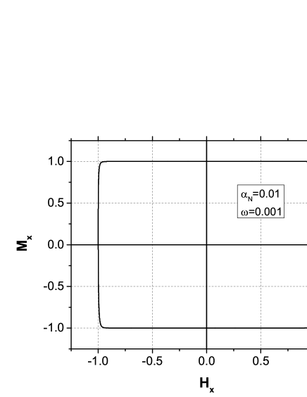
Figure 3: Dynamical hysteresis loop based on the solution (23) of the deterministic LLG equation with the following parameters, $\alpha_{N}$ = 0.01, $\omega_{L}$ = 0.2 and $\omega$ = 0.001. Its stochastic version is plotted on Fig. 8.

In order to obtain realistic results one has to use the stochastic LLG equation where thermal fluctuations are taken into account. By this modification one can see whether one retrieves the expected hysteresis loops usov_hysteresis .

III.3 Parallel static field, oscillating case

Let us now turn to the study of the case where the static field is chosen to be parallel to the direction of oscillation:

$${\bf H}_{\rm{eff}}=H\,\,\Big{(}\cos(\omega t)+b_{0},\,\,0,\,\,0\Big{)}.$$ (24)

For this configuration of the applied field, the analytic solution of the deterministic LLG equation is still possible and it reads as follows for the x-component of the magnetization vector

$$M_{x}(t) = \frac{(M_{x0}-1)+(M_{x0}+1)\exp{\left[\frac{2\alpha_{N}}{\omega}(\sin(\omega t)+b_{0}\omega t)\right]}}{(1-M_{x0})+(M_{x0}+1)\exp{\left[\frac{2\alpha_{N}}{\omega}(\sin(\omega t)+b_{0}\omega t)\right]}}.$$ (25)

The most important property of the solution (25) is its asymptotic behaviour:

$${{\mathrm{if}}}\,\,b_{0}>0,\,\,\,M_{x}(t\to\infty)=+1,\hskip 28.45274pt{{\mathrm{if}}}\,\,b_{0}<0,\,\,\,M_{x}(t\to\infty)=-1,$$ (26)

which can be seen as a fixed point solution in the laboratory frame, i.e., it is a time-independent steady state solution.

Consequently, the energy loss is basically vanishing according to the energy loss formula (15). In other words, for $t\to\infty$ the energy loss/cycle is non-zero only for $b_{0}=0$, see Fig. 4.

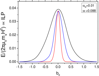
Figure 4: (Color online.) Energy loss/cycle as a function of the static field as based on (25) calculated in different cycles with $\alpha_{N}=0.01$ and $\omega=0.088$, i.e., for $t\to\infty$ the peak becomes sharper.

This suggests a very sharp superlocalization effect. The combination of parallel static and oscillating fields results in no energy loss for any non-vanishing values of the static field. However, this picture is based on the time-independent steady state solution of the deterministic LLG equation and one may expect a modification due to thermal effects for small static field values.

III.4 Perpendicular static field, oscillating case

Let us now investigate the case where the static field is chosen to be perpendicular to the direction of oscillation:

$${\bf H}_{\rm{eff}}=H\,\,\Big{(}\cos(\omega t),\,\,b_{0},\,\,0\Big{)}.$$ (27)

For this configuration of the applied field, we rely on numerical solutions. We observe that for $t\to\infty$ the solution tends to a time-dependent steady state, which can be seen as a limit cycle in the laboratory frame. The (time-dependent) steady state solution is periodic (typically contains higher harmonics) and it depends on the parameters $\omega,\omega_{L},\alpha_{N}$. Since it can be seen as an attractive solution, i.e., the magnetization vector always tends to this steady state motion independently of its initial value.

Thus, the energy loss can be calculated by simply taking into account only this steady state motion. For the considered values of $\omega,\omega_{L},\alpha_{N}$ one finds a single peak in the energy loss at $b_{0}=0$, see Fig. 5. This indicates that similarly to the previous case, the vanishing static field is favoured, which again results in superlocalization.

Figure 5: Energy loss/cycle as a function of $b_{0}$ obtained for the case where the static field is perpendicular to the line of oscillation with parameters $\alpha_{N}=0.01$, $\omega_{L}=0.2$ and $\omega=0.001$.

In summary, the solution of the deterministic LLG equation for the oscillating cases signals a drastic decrease in the energy loss in the presence of a non-vanishing static magnetic field independently of its orientation. However, this finding needs a careful re-examination around the small values of the static field where thermal fluctuations are present, since they can have a huge impact on the motion of the magnetization vector. Indeed, if one would like to obtain reliable hysteresis loops, the use of the stochastic LLG equation is unavoidable. Therefore, we investigate the solution of the stochastic LLG equation in the next section.

IV Stochastic Landau-Lifshitz-Gilbert equation

Let us now turn to our main goal and study the stochastic LLG equation (10) in the presence of the applied magnetic fields (3), (4) and (5), which are combinations of static and alternating ones.

IV.1 Rotating case

Let us first consider how the thermal fluctuations modify the steady state solutions. In Fig. 6 we show how the limit-cycle of Fig. 1 obtained by the solution of the stochastic LLG equation (10) for the temperature $T=300$K.

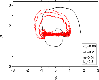
Figure 6: (Color online.) The same as Fig. 1, but now with non-vanishing temperature, i.e., this figure is obtained by the solution of the stochastic LLG equation (10) using the parameters and initial values of the results shown in Fig. 1 and $T=300$K.

The next step is to study if and how the thermal fluctuations change the energy loss obtained for the rotating case. In other words, we aim at studying the modifications of Fig. 2 by thermal effects. Fig. 7 shows the influence of thermal fluctuations on the enhancement and superlocalization effects reported in the case of the deterministic LLG equation (2).

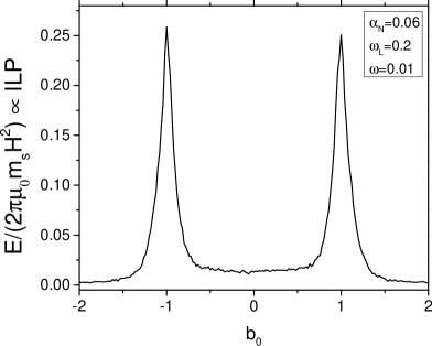
Figure 7: The same as Fig. 2, but now with non-vanishing temperature ($T=300$K), i.e., this figure is obtained by the solution of the stochastic LLG equation (10) using the parameters of Fig. 2 and averaged over $15$ cycles. The energy loss/cycle is plotted in terms of the parameter $b_{0}$.

The most important conclusion is that the deterministic (see Fig. 2) and the stochastic (see Fig. 7) results are very similar to each other. Thermal effects do not substantially spoil the enhancement and superlocalization effect for the rotating case. This is because the energy loss is calculated by using the (time-dependent) steady state solution of the LLG equations (for the deterministic and the stochastic cases) and these steady state solutions are attractive ones, so, the magnetization vector always tends to them. It follows that thermal fluctuations are not able to significantly modify the dynamics.

IV.2 Vanishing static field, oscillating case

Regarding the oscillating case, as a first step, we plot the dynamical hysteresis loop obtained for the vanishing static field case, but now with thermal effects taken into account, see Fig. 8, with the parameters $\alpha_{N}=0.01,\omega_{L}=0.2$, $\omega=0.001$ and $T=300$K.

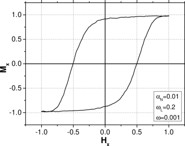
Figure 8: The same as Fig. 3 but for the stochastic version. The hysteresis loop is obtained by the stochastic LLG equation averaged over $50$ runs with $\alpha_{N}=0.01$, $\omega_{L}=0.2$, $\omega=0.001$ and $T=300$K.

This is the expected usual form of the hysteresis loop usov_hysteresis , where the dynamics of the magnetization is averaged out. This represents a drastic modification compared to the deterministic hysteresis loop. The reason for such significant change is the absence of time-dependent steady state solutions. In other words, the deterministic case is found to be an artifact since for any non-vanishing temperature the deterministic picture is spoiled by thermal effects. Thus the only way to obtain realistic results for the energy loss when no time-dependent steady state motion exits is to use the stochastic LLG equation (10).

IV.3 Parallel static field, oscillating case

As second step, we solve the stochastic LLG equation (10) in the presence of the applied magnetic field (4), which stands for a parallel combination of static and oscillating fields. We plot in Fig. 9 the energy loss as a function of the static field (for the the same set of parameters as before) for parallel orientations.

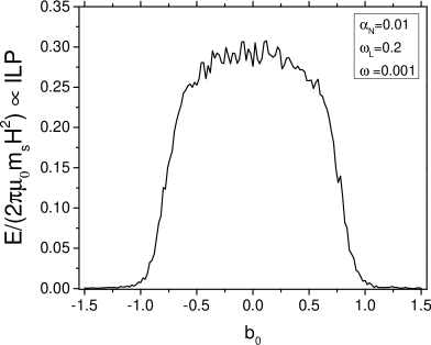
Figure 9: Energy loss as a function of the parallel static field amplitude obtained by the stochastic LLG equation averaged over thirty four cycles with $\alpha_{N}=0.01$, $\omega_{L}=0.2$, $\omega=0.001$ and $T=300$K.

Similarly to the case of vanishing static field, again thermal effects change drastically the dependence of the energy loss on the static field $b_{0}$ as seen if one compares Fig. 4 and Fig. 9. The deterministic case predicts no energy loss for any non-vanishing value for $b_{0}$ (in the limit of $t\to\infty$), but the stochastic result changes this picture for relatively small values of $b_{0}$. The reason for such significant modification is again the absence of time-dependent steady state solutions. Of course, large enough static field keeps aligned the magnetic moments, which results in a vanishing energy loss anyway.

IV.4 Perpendicular static field, oscillating case

We solve now the stochastic LLG equation (10) in the presence of the applied magnetic field (5), which stands for a perpendicular combination of static and oscillating fields. The energy loss as a function of the static field is plotted for perpendicular orientations in Fig. 10.

Figure 10: Energy loss as a function of the perpendicular static field amplitude obtained by the stochastic LLG equation averaged over fourteen cycles with $\alpha_{N}=0.01$, $\omega_{L}=0.2$, $\omega=0.001$ and $T=300$K.

In this case, thermal fluctuations only slightly modify the deterministic results. The stochastic description confirms that with static field oscillating applied fields are not favoured, i.e., the largest energy loss can be achieved by the vanishing static field.

IV.5 Discussion

In summary, thermal effects are found to be important for those cases only where the deterministic LLG equation has no time-dependent steady state solutions. These are the cases of vanishing and parallel static field configuration for oscillation. At variance, thermal fluctuations have no significant effects if the static field is in the plane of rotation or perpendicular to the line of oscillation, a case in which the deterministic (and stochastic) LLG equation has time-dependent steady state solutions. Thus, thermal effects have an important impact on superlocalization. We find that based on the results obtained from the stochastic LLG, the superlocalization effect of the deterministic case for oscillating fields in presence of a parallel static field does not hold, while it is conserved in the other considered cases: rotating fields with an in plane static field and oscillating field with a perpendicular static field.

V Heating efficiency of rotating and oscillating cases

Let us compare the maximum heating efficiency or more precisely the ILP and SAR values of the rotating and oscillating cases paying attention on the superlocalization effect too. In order to achieve maximum energy loss for the rotating case, the static field should be in the plane of rotation and its amplitude should be identical to that of the rotating field (for isotropic, i.e., spherically symmetric nanoparticles). For the oscillating field, the static field should vanish to achieve the maximum energy loss.

V.1 Variable frequency and fixed amplitude for the applied field

We can compare four cases: results obtained for oscillating applied fields with vanishing static field for $T=0$ and $T\neq 0$; and findings for the rotating case with in-plane static field (with $|b_{0}|=1$) for $T=0$ and $T\neq 0$.

The dependence of the energy loss/cycle on the applied (dimensionless) frequency is plotted for the above mentioned four cases in Fig. 11. We remind that the dimensionless parameters are defined by (II) and a typical value for the dimensionless frequency suitable for hyperthermia is $\omega\sim 10^{-4}$. It is clear from Fig. 11 that for the application of hyperthermia one should consider the low frequency limit of the four curves, which is plotted in Fig. 12.

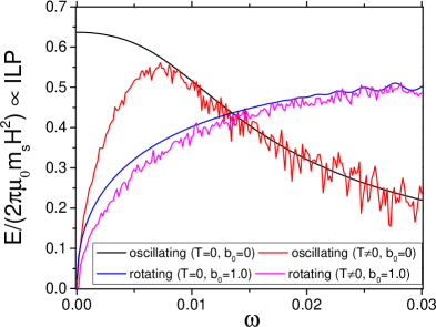
Figure 11: (Color online.) Dependence of the energy loss/cycle on the applied (dimensionless) frequency averaged over eightyfour cycles with parameters $\alpha=0.1$, $\alpha_{N}=0.02,\omega_{L}=0.2$ and $T=300$K.

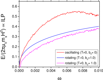
Figure 12: (Color online.) Same as Fig. 11, but for the low-frequency limit.

We observe that a similar figure can be found in Raikher_Stephanov , see Fig. 6 therein where oscillating and rotating cases are compared, but without any static field. In addition, to check the stochastic solver, we compare our numerical data obtained for the pure oscillating case (with no static field) to existing theoretical and experimental results in Appendix B.

Static field is of great importance for the rotating case since in-plane static field can give raise to a drastic enhancement of the heating efficiency. Therefore the conclusions of Raikher_Stephanov has to be examined in presence of a (possibly small) in-plane static field, a re-examination which is done here.

For the oscillating case (in the absence of static fields) the stochastic results substantially modify for very low frequencies the picture emerging from the deterministic LLG. In the previous section we discussed in detail the reason for that and the explanation is related to the absence of time-dependent steady state motions, which results in an artifact for the limit of $\omega\to 0$ of the deterministic case. In other words in case of the absence of (time-dependent) steady state motions, the athermal and low-frequency limits do not commute. This general statement is considered for the special case of oscillating external applied field in Raikher_Stephanov . Thus, for oscillation (without static field) it is very important to rely on the stochastic results.

For the rotating case with in-plane static field, thermal effects are at variance less important because the presence of attractive steady state motions. Thus, in this case one can rely on the deterministic results, however, for very low-frequencies the precise quantitative analysis requires the stochastic approach as shown in Fig. 12. The reason why the deterministic and the stochastic results are quantitatively different for the rotating case in the low-frequency limit is the following. If the magnitudes of the static and the rotating fields are identical which is the case for $|b_{0}|=1$ then the effective applied field varying in time drops to zero when the static and rotating fields have opposite directions and this happens once in each and every cycle. At this point the magnetisation vectors of the individual nanoparticles feel no external field and they start to diverge from each other due to thermal fluctuations. This effect is enhanced for low frequencies when the variation of the effective applied field in time is slow compared to thermal effects, so, the deterministic and the stochastic results start to differ from each other quantitatively. If the magnitudes of the static and the rotating fields are not identical, i.e., for $|b_{0}|\neq 1$, then the effective applied field never drops to zero, thus, one finds no difference between the deterministic and the stochastic results.

The rotating case produces a better heating efficiency for very large frequencies, but these are not suitable for hyperthermia. For smaller frequencies, the oscillating case becomes more favourable. For very low frequencies, see Fig. 13,

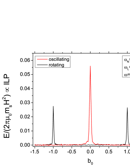
Figure 13: (Color online.) Comparison of the energy loss as a function of the static field amplitude for the oscillating and the rotating cases averaged over twenty four cycles. The static field is chosen to be perpendicular in the oscillating case and in-plane for the rotating applied field. The applied field magnitude is $H=18$kA/m, the applied frequency is chosen to be its maximum value $2\times 10^{6}$Hz, the dimensionless damping parameter is $\alpha=0.1$ and the temperature is $T=300$K.

the oscillating field for vanishing static field produces twice as much heating efficiency as that of the rotating one with in-plane static field with $|b_{0}|=1$. The reason is the following. We have discussed already that the effective applied field of the rotating case drops to zero when the static and rotating fields have opposite directions (and they have same magnitudes) and this happens once in each and every cycle. One can also show that the majority of the energy loss over a single cycle is observed when the effective field starts to grow up from zero. This is true for oscillating case, too. Thus, when the rotating field is combined with an in-plane static field with identical amplitudes, the resulting effective applied field acts very much like an oscillating one in the very low-frequency limit. The difference between the two cases is the fact that for the oscillating case the effective field drops to zero two times per cycle, thus, its heating efficiency is expected to be twice as much large as the combined rotating one. Indeed, this can be seen, if one compares the peaks in Fig. 13. However, it is not obvious that the oscillating case remains favourable for a different choice of the applied frequency and field strength keeping their product to be constant to support the Hergt-Dutz limit. Let us examine this in the next subsection.

V.2 Variable frequency and amplitude for the applied field

It is shown in Fig. 13 that the appropriate combination of rotating and (in-plane) static fields acts like an oscillating one (for relatively low frequencies) but in order to achieve the same heating efficiency or more precisely the same SAR one has to double the applied frequency. Thus, if one plots the SAR as a function of the ratio $r$ of the applied field strength (amplitude) $H$ and the angular frequency $\omega$ and keeping their product $H\omega=H_{\star}\omega_{\star}$ at a constant value,

$$r^{2}=\frac{H}{\omega}\frac{\omega_{\star}}{H_{\star}}\hskip 8.5359pt\to\hskip 8.5359ptr^{2}\equiv 1\,\,\,{\mathrm{for}}\,\,\,H_{\star}=18{\mathrm{kA/m}},\,\,\,\omega_{\star}=2\times 10^{6}{\mathrm{Hz}}\hskip 8.5359pt\to\hskip 8.5359ptr=\sqrt{\frac{\omega^{2}_{\star}}{\omega^{2}}}=\sqrt{\frac{H^{2}}{H^{2}_{\star}}}$$ (28)

one expects the same type of function for the oscillating and rotating cases but shifted by a factor of two, see Fig. 14.

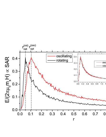
Figure 14: (Color online.) Comparison of the SAR as a function of the ratio $r$ given by (28) obtained for the oscillating (zero static field) and rotating (in-plane static field) cases averaged over fourteen cycles. One finds a single peak at $r^{{\mathrm{(rot)}}}_{{\mathrm{opt}}}=0.05$ for the rotating case and at $r^{{\mathrm{(osc)}}}_{{\mathrm{opt}}}=2\,\,r^{{\mathrm{(rot)}}}_{{\mathrm{opt}}}=0.1$ for the oscillating one. The inset shows that the two curves coincide if the SAR of the rotating case is plotted as a function of $2r$.

Indeed, on Fig. 14 we show the SAR as a function of the ratio $r$ and one finds a single maximum for the rotating and oscillating cases where the positions of the peaks are related to each other, $r^{{\mathrm{(osc)}}}_{{\mathrm{opt}}}=2\,\,r^{{\mathrm{(rot)}}}_{{\mathrm{opt}}}$. This demonstrates that in order to achieve the same heating efficiency, i.e., the same SAR for the rotating and oscillating cases, one has to double the applied frequency (more precisely the ratio $r$) of the rotating applied field compared to the oscillating one, so, in this case the SAR functions coincide, see the inset of Fig. 14.

The peaks suggest optimal choices for the applied frequency and field strength (amplitude) for the oscillating ($2\times 10^{7}$Hz, $1800$A/m) and for the rotating ($4\times 10^{7}$Hz, $900$A/m) cases. At these values, the SAR’s and ILP’s are the same, see Fig. 15.

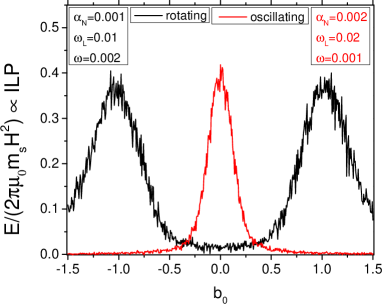
Figure 15: (Color online.) In this figure we show how the superlocalization effect presented on Fig. 13 is modified for smaller frequencies and larger field strength values averaged over thirty four cycles. We choose the following dimensionful parameters for the oscillating $2\times 10^{7}$Hz, $1800$A/m and for the rotating $4\times 10^{7}$Hz, $900$A/m cases.

One finds identical SAR and ILP values for the rotating and the oscillating cases but at different frequencies and different field amplitudes. In particular, for smaller field amplitudes and for higher frequencies the combination of the rotating and in-plane static fields seems to be a better choice, i.e., it gives larger SAR. However, we have two important comments. First, the superlocalization effect is weakened compared to the case discussed in the previous subsection where the frequency was smaller ($2\times 10^{6}$Hz), and the field strength was larger ($18$kA/m). Second, one has to keep the applied frequency below the the eddy current threshold, so the maximum applied frequency cannot exceed 1000 kHz (under any circumstances), thus, the peaks of the SAR graphs cannot be used in medical applications.

Instead of the SAR, it is more reliable to study the ILP values, see, Fig. 16 which has huge importance in technical realisation.

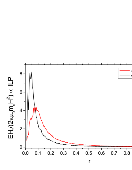
Figure 16: (Color online.) The same as Fig. 14, but for the ILP values.

The ILP values of Fig. 16 show that in the low frequency (large $r$) regime suitable for hyperthermia, the oscillating applied field is shown to result in two times larger ILP then the rotating one with identical superlocalization ability which has importance in technical realisation.

Let us note that we expect that the above findings do not depend on the maximum choice of the product of the frequency and field strength $\omega_{\star}H_{\star}$. This is because the deterministic LLG equation is invariant under the appropriate simultaneous rescaling of $\omega$, $H$ and the time variable $t$, thus these quantities are related to each other, so one can draw some conclusions on from Fig. 14 and Fig. 16 for other values of the product $\omega_{\star}H_{\star}$.

VI Summary and Conclusions

In this work we considered theoretically whether and how thermal effects can modify the enhancement of heat transfer and the superlocalization effect of magnetic nanoparticle hyperthermia for oscillating and rotating applied fields. Furthermore, we compared the efficiency and superlocalization of the rotating and oscillating cases.

It is known that if the amplitudes of the (in-plane) static and rotating applied fields fulfil a certain relation (they should be identical for the isotropic case), then the energy transfer from the applied field into the environment is found to be enhanced drastically. In addition, by using an inhomogeneous static field one can induce superlocalization. Another example for superlocalization is the combination of an applied oscillating and a static field gradient, which provides a spatially focused heating since for large enough static field the dissipation drops to zero, so, the temperature increase is observed only where the static field vanishes.

It is a relevant question to ask whether thermal effects modify the sharpness of superlocalization. Therefore for experiments, i.e., application in tumor-therapy, thermal fluctuations have to be taken into account. Thus, it is required to study these issues by the stochastic Landau-Lifshitz-Gilbert (LLG) equation, whose investigation is presented here.

We obtained that when time-dependent steady state motions are present, then deterministic and stochastic results are very similar to each other. This is found in the rotating case with in-plane static field and in the oscillating case with perpendicular static field. However, in the absence of these time-dependent steady state motions, the efficiency of the method and its superlocalization suffers drastic modifications by thermal effects. This occurs for the oscillating case with vanishing and parallel static fields.

Our most important result is that comparing the most efficient rotating and oscillating combinations, we found that for smaller field amplitudes and for higher frequencies the combination of the rotating and in-plane static fields seems to be a better choice, i.e., it gives larger ILP and SAR values however, these high frequencies are unacceptable for medical applications. In the low-frequency range suitable for magnetic hyperthermia, the oscillating applied field was shown to result in two times larger ILP and SAR then the rotating one with identical superlocalization ability which has importance in technical realisation.

In particular, we showed that one finds identical SAR values for the rotating and the oscillating cases but at different frequencies and different field amplitudes. In other words, if one compares the rotating and oscillating applied fields at the same frequency suitable for medical applications, the latter produces us a better heating efficiency. This theoretical result holds with only one condition, namely that the energy loss over the cycle must be localised to the time-domain when the applied field starts to increase from its zero value, so thus the appropriate combination of rotating and (in-plane) static fields acts like an oscillating one.

In summary, we demonstrated that the combination of static and rotating fields can have importance in technical realisation of magnetic nanoparticle hyperthermia but keeping in mind that it has a worse heating efficiency compared to the usual oscillating one in the frequency range suitable for medical applications.

Of course, in order to look for the most efficient applied field configuration, one can perform further theoretical investigations. For example, open questions motivated by the present theoretical study of the enhancement and superlocalization effects are the inclusion of (i) the interaction between the particles which can results in formation of clusters usov_claster ; (ii) the dependence on the diameter of the nanoparticles; and (iii) the possible rotating motions of the nanoparticle as a whole lyutyy_general ; joined_motion ; joined_motion_bis_1 ; joined_motion_bis_2 ; joined_motion_2 ; thermal_and_dipole ; viscous_rotating . However, we do expect that considerations very likely do not violate our major finding that appropriate combination of rotating and (in-plane) static fields is essentially like an oscillating one but in order to achieve the same heating efficiency, i.e., the same SAR one has to double the applied frequency, so, for the same frequency, the oscillating combination is a better choice.

Based on our results, we suggest targeted experimental studies incorporating standardized techniques standardized_techniques ; wildeboer_r_r . For example, we propose to use well separated isotropic nanoparticles in an aerogel matrix where only the magnetic moment can rotate. There are proposals for the technical realisation of a rotating applied field, see, e.g., exp_rot and non_calorimetric . For example, in exp_rot the authors discuss possible experimental realisation of generating a rotating applied field. The standard choice could be a system of two pairs of Helmholtz coils whose axes are perpendicular to each other but in exp_rot the authors suggest a system of three pairs of inductors connected in series with capacitors to generate a rotary magnetic field. This configuration (with the inclusion of a static field) can be directly used to test theoretical predictions of the present work. Also non-calorimetric technics highly_accurate , non_exp_relax are used to measure the energy losses in various applied fields. In non_calorimetric , the authors present the validation of a resonators with a so-called birdcage coil. This represents another realisation of rotating magnetic field. Again, with the inclusion of a static field on can test our numerical results obtained for the rotating field case. In addition, one can discuss possible experimental realisation to measure the decrease of heat generation as a function of the static field. For example, a possible measurement setup could be when a rotatable resonator is placed into the electromagnet which generates the static field. In this manner, one can easily perform measurements for the case when the oscillating filed and the static one are perpendicular or parallel to each other. Thus, the predictions of the present work can be tested with the help of the required combinations of static and alternating applied fields.

Appendix A Consistency checks of the stochastic LLG equation

In this Appendix we present some consistency checks based on the numerical results discussed Giordano . In section VI of Giordano the magnetization dynamics of an anisotropic nanoparticle has been studied in the absence of any applied field and the anisotropy field is assumed to be parallel to the z-axis (by using uniaxial shape anisotropy):

$${\bf H}_{\rm{eff}}={\bf H}_{\rm{a}}=H\,\,(0,0,\lambda_{\rm{eff}}M_{z}),$$ (29)

where $\lambda_{\rm{eff}}=H_{a}/H$ is the anisotropy ratio and $H_{a}$ is the anisotropy field. In the spherical coordinate system the stochastic LLG equation (10) takes the form

$$\frac{\rm{d}}{\rm{d}t}\phi =-\omega_{L}\lambda_{\rm{eff}}\cos\theta+\frac{1}{\sin\theta}\sqrt{\frac{1}{2\tau_{N}}}n_{\phi},$$ (30)

$$\frac{\rm{d}}{\rm{d}t}\theta =-\alpha_{N}\lambda_{\rm{eff}}\cos\theta\sin\theta+\frac{1}{2\tau_{N}}\frac{\cos\theta}{\sin\theta}+\sqrt{\frac{1}{2\tau_{N}}}n_{\theta},$$ (31)

where $n_{\phi}$ and $n_{\theta}$ satisfy the relations given in (14). The above stochastic differential equations are identical to Eq. (27) of Giordano . To have a more clear picture, these can be rewritten to the standard form of an Ito process $\mathrm{d}X=b(X)\,\mathrm{d}t+\sigma\,\mathrm{d}W$. From (14) one can observe that the variance of $n_{\phi(\theta)}$ is multiplied by a factor of 2, which can be explicitly written as a $\sqrt{2}$ multiplicative factor of the Wiener process. Thus the full stochastic process in the standard form writes as

$$\rm{d}\phi =-\omega_{L}\lambda_{\rm{eff}}\cos\theta\;\rm{d}t+\frac{1}{\sin\theta}\sqrt{\frac{1}{2\tau_{N}}}\sqrt{2}\;\rm{d}W_{1},$$ (32)

$$\rm{d}\theta =\left(-\alpha_{N}\lambda_{\rm{eff}}\cos\theta\sin\theta+\frac{1}{2\tau_{N}}\frac{\cos\theta}{\sin\theta}\right)\rm{d}t+\sqrt{\frac{1}{2\tau_{N}}}\sqrt{2}\;\rm{d}W_{2},$$ (33)

where $\rm{d}W_{1}$ and $\rm{d}W_{2}$ are independent Wiener processes with the standard normal distribution. This Ito process can be directly solved by the built-in functions of Mathematica wolfram , where the time is discretized. In this case setting the numerical time step ${\rm{d}t}=1.5\times 10^{-10}s$ produces reliable results. At each time step, $\rm{d}\phi$ and $\rm{d}\theta$ receives a random, normal distributed ’kick’ from the $\rm{d}W$ terms centered around zero with a variance that is adjusted by the size of the time step $\sigma^{2}_{W}=\rm{d}t$. Fig. 6 of Ref. Giordano contains some details regarding the average values of the Cartesian components of the magnetization vector. Therefore it is illustrative to recover this known result by our stochastic solver using the same values for the parameters $\tau_{N}=1.5\times 10^{-7}$s, $\omega_{L}\lambda_{\rm{eff}}=2.58\times 10^{8}$s^-1, $\alpha_{N}\lambda_{\rm{eff}}=7.74\times 10^{7}$s^-1, results from which are presented in Fig. 17. The comparison confirms the validity of the numerical method used here for the stochastic solver.

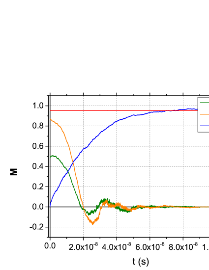
Figure 17: (Color online.) In this figure we plot the average values of $M_{x}(t)$ (green curve), $M_{y}(t)$ (yellow curve) and $M_{z}(t)$ (blue curve) are plotted versus the time where the horizontal red line stands for the asymptotic value given in Ref. Giordano (compare it in particular with the central panel of Fig. 6 in Ref. Giordano ).

Appendix B Consistency check of the results

In order to check our theoretical results based on the stochastic LLG equation, we determine the imaginary part of the AC susceptibility obtained for the pure oscillating (without static) external field and compare it to the corresponding literature both on the theory and the experimental side. The frequency dependence of the AC susceptibility is given by

$$\chi^{\prime\prime}(\omega)=\chi_{0}\frac{\omega\tau}{1+\omega^{2}\tau^{2}}$$ (34)

see for example Eq.(4) and (5) of non_exp_relax . This form is valid when a single relaxation process is present only. In our case the frequency dependence is characterised by the Néel relaxation time, $\tau=\tau_{N}$, since we investigated small enough nanoparticles to neglect their rotation inside their environment and only the Néel process, i.e, the rotation of the magnetisation is taken into count.

We use the formula (34) to fit our theoretical results obtained by the stochastic LLG equation for the pure oscillating case. On Fig. 18 the solid line denotes the fitted curve which gives the following fitted relaxation time, $\tau_{N}=157\times 0.5\times 10^{-10}{\mathrm{s}}\sim 0.78\times 10^{-8}{\mathrm{s}}$ and the following fitted magnitude, $\chi_{0}=1.09$.

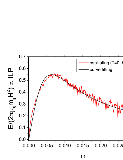
Figure 18: (Color online.) In this figure we plot the imaginary parts of the AC susceptibility (which is related to ILP) as a function of the applied (dimensionless) frequency for pure oscillating case. Numerical data are identical to the red curve of Fig. 11. The solid line is a fitted curve to numerical data based on (34).

We conclude that our numerical results obtained by the stochastic LLG equation can be well described by the standard formula (34). In addition, the relaxation time calculated by the fitting procedure, $\tau_{N}\sim 1$ ns is in the range of typical value for magnetic nanoparticles, see e.g., ota . Finally, we argue that our results are in agreement with known experimental results, see for example, Fig.2 of ferguson .

References

- (1) Pankhurst, Q. A.; Connolly, J.; Jones, S. K.; Dobson, J. Applications of magnetic nanoparticles in biomedicine. J. Phys. D: Appl. Phys. 2003, 36, R167.
- (2) Ortega, D.; Pankhurst, Q.A. Magnetic hyperthermia. Nanoscience 2003 1, e88.
- (3) Pankhurst, Q. A.; Thanh, N. T. K.; Jones, S. K.; Dobson, J. Progress in applications of magnetic nanoparticles in biomedicine. J. Phys. D: Appl. Phys. 2003, 42, 224001.
- (4) Perigo, E. A.; Hemery, G.; Sandre, O.; Ortega, D.; Garaio, E.; Plazaola, F.; Teran, F. J. Fundamentals and advances in magnetic hyperthermia. Appl. Phys. Rev. 2015, 2, 041302.
- (5) Cabrera, D.; Camarero, J.; Ortega D.; Teran, F. J. Influence of the aggregation, concentration, and viscosity on the nanomagnetism of iron oxide nanoparticle colloids for magnetic hyperthermia. J. Nanopart. Res. 2015, 17, 121.
- (6) Thiesen, B.; Jordan, A.; Clinical applications of magnetic nanoparticles for hyperthermia. Int. J. Hyperthermia 2008, 24, 467-474.
- (7) Wust, P.; Gneveckow, U.;, Johannsen, M.; et al. Magnetic nanoparticles for interstitial thermotherapy, feasibility, tolerance and achieved temperatures. Int. J. Hyperthermia 2006, 22, 673-685.
- (8) Creixell, M.; Bohorquez, A. C.; Torres-Lugo, M.; Rinaldi, C. EGFR-Targeted Magnetic Nanoparticle Heaters Kill Cancer Cells without a Perceptible Temperature Rise. ACS Nano 2011, 5, 7124
- (9) Domenech, M.; Marrero-Berrios, I.; Torres-Lugo, M.; Rinaldi, C. Lysosomal membrane permeabilization by targeted magnetic nanoparticles in alternating magnetic fields. ACS nano 2013, 7, 5091-5101.
- (10) Chiu-Lam, A.; Rinaldi, C. Nanoscale Thermal Phenomena in the Vicinity of Magnetic Nanoparticles in Alternating Magnetic Fields. Adv. Funct. Mater. 2016, 26, 3933-3941.
- (11) Weber, C.; Morsbach, S.; Landfester, K. Possibilities and Limitations of Different Separation Techniques for the Analysis of the Protein Corona. Angew. Chem. 2019, 58, 12787-12794.
- (12) Dhavalikar, R.; Bohorquez, A. C.; Rinaldi, C. Image-Guided Thermal Therapy Using Magnetic Particle Imaging and Magnetic Fluid Hyperthermia. Nanomaterials for Magnetic and Optical Hyperthermia Applications, Micro and Nano Technologies 2019, 265-286.
- (13) Kut, C.; Zhang, Y.; Hedayati, M.; Zhou, H.; Cornejo, C.; Bordelon, D.; Mihalic, J.; Wabler, M.; Burghardt, E.; Gruettner, C.; Geyh, A.; Brayton, C.; Deweese, T. L.; Ivkov, R. Preliminary study of injury from heating systemically delivered, nontargeted dextran superparamagnetic iron oxide nanoparticles in mice. Nanomedicine 2012, 7, 1697.
- (14) Tay, Z. W.; Chandrasekharan, P.; Chiu-Lam, A.; Hensley, D. W.; Dhavalikar, R.; Zhou, X. Y.; Yu, E. Y.; Goodwill, P. W.; Zheng, B.; Rinaldi, C.; Conolly, S. M. Magnetic Particle Imaging-Guided Heating in Vivo Using Gradient Fields for Arbitrary Localization of Magnetic Hyperthermia Therapy. ACS Nano 2018, 12, 3699-3713.
- (15) Tasci, T. O.; Vargel, I.; Arat, A.; Guzel, E.; Korkusuz, P.; Atalar, E. Focused RF hyperthermia using magnetic fluids. Med. Phys. 2009, 36, 1906-1912.
- (16) Ho, S. L.; Jian, L.; Gong, W.; Fu, W.N. Design and Analysis of a Novel Targeted Magnetic Fluid Hyperthermia System for Tumor Treatment. IEEE Trans. Magn. 2012, 48, 3262-3265.
- (17) Ho, S. L.; Niu, S.; Fu, W. N. Design and Analysis of Novel Focused Hyperthermia Devices. IEEE Trans. Magn. 2012, 48, 3254-3257.
- (18) Ma, M.; Zhang, Y.; Shen, X.; Xie, J.; Li, Y.; Gu, N. Targeted inductive heating of nanomagnets by a combination of alternating current (AC) and static magnetic fields. Nano Res. 2015, 8, 600-610.
- (19) Hensley, D.W.; Tay, Z.W.; Dhavalikar, R.; Zheng, B.; Goodwill, P.; Rinaldi, C.; Conolly, S. Combining magnetic particle imaging and magnetic fluid hyperthermia in a theranostic platform. Phys. Med. Biol. 2017, 62, 3483.
- (20) Dhavalikar, R.; Rinaldi, C. Theoretical predictions for spatially-focused heating of magnetic nanoparticles guided by magnetic particle imaging field gradients. J. Magn. Magn. Mater. 2016, 419, 267-273.
- (21) Iszály, Zs.; Lovász, K.; Nagy, I.; Márián, I. G.; Rácz, J.; Szabó, I. A.; Tóth, L.; Vas, N. F.; Vékony, V.; Nándori, I. Efficiency of magnetic hyperthermia in the presence of rotating and static fields. J. Magn. Magn. Mater. 2018, 466, 452-462.
- (22) Kim, M.-K.; Sim, J.; Lee, J.-H.; Kim, M.; Kim, S.-K. Dynamical Origin of Highly Efficient Energy Dissipation in Soft Magnetic Nanoparticles for Magnetic Hyperthermia Applications. Phys. Rev. Appl. 2018, 9, 054037.
- (23) Bertotti, G.; Serpico C.; Mayergoyz, I. D. Nonlinear Magnetization Dynamics under Circularly Polarized Field. Phys. Rev. Lett. 2001, 86, 724.
- (24) Denisov, S. I.; Lyutyy, T. V.; Hänggi, P. Magnetization of Nanoparticle Systems in a Rotating Magnetic Field. Phys. Rev. Lett. 2006, 97, 227202.
- (25) Denisov, S. I.; Lyutyy, T. V.; Hänggi, P.; Trohidou, K. N. Dynamical and thermal effects in nanoparticle systems driven by a rotating magnetic field. Phys. Rev. B 2006, 74, 104406.
- (26) Cantillon-Murphy, P.; Wald, L.L.; Adalsteinsson, E.; Zahn, M. Heating in the MRI environment due to superparamagnetic fluid suspensions in a rotating magnetic field. J. Magn. Magn. Mater. 2010, 322, 727-733.
- (27) Ahsen, O. O.; Yilmaz, U.; Aksoy, M. D.; Ertas, G.; Atalar, E. Heating of magnetic fluid systems driven by circularly polarized magnetic field. J. Magn. Magn. Mater. 2010, 322, 3053-3059.
- (28) Denisov, S. I.; Lyutyy, T. V.; Binns, C.; Hänggi, P. Phase diagrams for the precession states of the nanoparticle magnetization in a rotating magnetic field. J. Magn. Magn. Mater. 2010, 322, 1360-1362.
- (29) Denisov, S. I.; Polyakov, A. Yu.; Lyutyy, T. V. Resonant suppression of thermal stability of the nanoparticle magnetization by a rotating magnetic field. Phys. Rev. B 2011, 84, 174410.
- (30) Raikher Yu. L.; Stephanov, V. I. Power losses in a suspension of magnetic dipoles under a rotating field. Phys. Rev. E 2011, 83, 021401.
- (31) Chen, S.-W.; Lai, J.-J.; Chiang, C.-L.; Chen, C.-L. Construction of orthogonal synchronized bi-directional field to enhance heating efficiency of magnetic nanoparticles. Review of Scientific Instruments 2012, 83, 064701.
- (32) Lyutyy, T. V.; Denisov, S. I.; Polyakov, A. Yu.; Binns, C. Power Loss of the Nanoparticle Magnetic Moment in Alternating Fields. Nanomaterials: Applications and Properties (NAP-2012): 2-nd International conference 2012, 1, 04MFPN16.
- (33) Lyutyy, T. V.; Denisov, S. I.; Peletskyi, A. Yu.; Binns, C. Energy dissipation in single-domain ferromagnetic nanoparticles: Dynamical approach. Phys. Rev. B 2015, 91, 054425.
- (34) Skumiel, A.; Leszczynski, B.; Molcan, M.; Timko, M. The comparison of magnetic circuits used in magnetic hyperthermia. J. Magn. Magn. Mater. 2016, 420, 177-184.
- (35) Lyutyy, T. V.; Hryshko, O. M.; Kovner, A. A. Power loss for a periodically driven ferromagnetic nanoparticle in a viscous fluid: The finite anisotropy aspects. J. Magn. Magn. Mater. 2018, 446, 87-94.
- (36) Phong, P.T.; Nguyen, L.H.; Lee, I.J; Phuc, N.X; Computer simulations of contributions of Néel and Brown relaxation to specific loss power of magnetic fluids in hyperthermia. J. Electron. Mater. 2017, 46, 2393-2405
- (37) Usov, N. A.; Rytov, R. A.; Bautin, V. A. Dynamics of superparamagnetic nanoparticles in viscous liquids in rotating magnetic fields. Beilstein J. Nanotechnol. 2019, 10, 2294
- (38) Hergt, R.; Andra, W.; d’Ambly, C.; Hilger, I.; Kaiser, W.; Richter U.; Schmidt, H. Physical limits of hyperthermia using magnetite fine particles. IEEE Trans. Magn. 1998, 34, 3745
- (39) Hergt, R.; Dutz, S.; Zeisberger, M. Validity limits of the Néel relaxation model of magnetic nanoparticles for hyperthermia. Nanotechnology 2010, 21, 015706.
- (40) Hergt, R.; Dutz, S. Magnetic particle hyperthermia: biophysical limitations of a visionary tumour therapy. J. Magn. Magn. Mater. 2007, 311, 187-192.
- (41) Gneveckow, U.; Jordan, A.; Scholz, R.; Bruss, V.; Waldofner, N.; Ricke, J.; Feussner, A.; Hildebrandt, B.; Rau, B.; Wust, P. Description and characterization of the novel hyperthermia and thermoablation system for clinical magnetic fluid hyperthermia. Med. Phys. 2004, 31, 1444-1451.
- (42) Thiesen, B.; Jordan, A. Clinical applications of magnetic nanoparticles for hyperthermia. Int. J. Hyperth. 2008, 24, 467-474.
- (43) Landau L.; Lifshitz, E. On the theory of the dispersion of magnetic permeability in ferromagnetic bodies. Phys. Z. Sowjetunion 1935, 8, 153
- (44) Gilbert, T. L. A Lagrangian formulation of the gyromagnetic equation of the magnetization field. Phys. Rev. 1955, 100, 1243.
- (45) Brown, W. F. Thermal Fluctuations of a Single-Domain Particle. Phys. Rev. 1963, 130, 1677.
- (46) Brown, W. Thermal fluctuation of fine ferromagnetic particles. IEEE Trans. Magn. 1979, 15, 1196 - 1208.
- (47) Bordelon D; Cornejo C; Grüttner C; Westphal F; DeWeese T. L.; Ivkov R, Magnetic nanoparticle heating efficiency reveals magneto-structural differences when characterized with wide ranging and high amplitude alternating magnetic fields, J. Appl. Phys. 109, 124904, (2011) .
- (48) Fannin, P. C.; Malaescue, I.; Marin, C. N. The effective anisotropy constant of particles within magnetic fluids as measured by magnetic resonance. J. Magn. Magn. Mater. 2005, 289, 162-164.
- (49) Rácz, J.; de Châtel, P. F.; Szabó, I. A.; Szunyogh, L.; Nándori, I. Improved efficiency of heat generation in nonlinear dynamics of magnetic nanoparticles. Phys. Rev. E 2016, 93, 012607.
- (50) Nándori I.; Rácz, J. Magnetic particle hyperthermia: Power losses under circularly polarized field in anisotropic nanoparticles. Phys. Rev. E 2012, 86, 061404.
- (51) de Châtel, P. F.; Nándori, I.; Hakl, J.; Mészáros, S.; Vad, K. Magnetic particle hyperthermia: Néel relaxation in magnetic nanoparticles under circularly polarized field. J. Phys.: Condens. Matter 2009, 21, 124202.
- (52) Giordano, S.; Dusch, Y.; Tiercelin, N.; Pernod, P.; Preobrazhensky, V. Stochastic magnetization dynamics in single domain particles. Eur. Phys. J. B 2013, 86, 249.
- (53) Aron, C.; Barci, D. G.; Cugliandolo, L. F.; Arenas, Z. G.; Lozano, G. S. Magnetization dynamics: path-integral formalism for the stochastic Landau-Lifshitz-Gilbert equation. J. Stat. Mech. 2014, P09008.
- (54) Grozdanov S.; Polonyi, J. Viscosity and dissipative hydrodynamics from effective field theory. Phys. Rev. D 2015, 91, 105031.
- (55) Nagy, S.; Polonyi, J.; Steib, I. Quantum renormalization group. Phys. Rev. D 2016, 93, 025008.
- (56) Wolfram Research, Inc., Mathematica, Champaign, IL 2021.
- (57) Mamiya, H.; Jeyadevan, B. Hyperthermic effects of dissipative structures of magnetic nanoparticles in large alternating magnetic fields. Sci. Rep. 2011, 1, 157.
- (58) Usov, N. A.; Liubimov, B. Y. Dynamics of magnetic nanoparticle in a viscous liquid: Application to magnetic nanoparticle hyperthermia. Journal of Applied Physics 2012, 112, 023901.
- (59) Usov, N. A.; Liubimov, B. Y. Magnetic nanoparticle motion in external magnetic field. J. Magn. Magn. Mater. 2015, 385, 339-346.
- (60) Usadel, K. D.; Usadel, C. Dynamics of magnetic single domain particles embedded in a viscous liquid. J. Appl. Phys. 2015, 118, 234303.
- (61) Kallumadil, M.; Tada, M.; Nakagawa, T.; Abe, M.; Southern, P.; Pankhurst, Q. A. Suitability of commercial colloids for magnetic hyperthermia. J. Magn. Magn. Mater. 2009, 321, 1509-1513.
- (62) Lyutyy, T. V.; Reva, V. V. Energy dissipation of rigid dipoles in a viscous fluid under the action of a time-periodic field: The influence of thermal bath and dipole interaction. Phys. Rev. E 2018, 97, 052611.
- (63) Usov, N. A.; Serebryakova, O. N.; Tarasov, V. P. Interaction Effects in Assembly of Magnetic Nanoparticles. Nanoscale Res. Lett. 2017, 12, 489.
- (64) Usov, N. A. Low frequency hysteresis loops of superparamagnetic nanoparticles with uniaxial anisotropy. J. Appl. Phys. 2010, 107, 123909.
- (65) Wells, J.; Ortega, D.; Steinhoff U.; Dutz, S.; Garaio, E.; Sandre, O.; Natividad, E.; Cruz, M. M.; Brero, F.; Southern, P.; Pankhurst, Q. A.; Spassov, S. and the RADIOMAG consortium, Challenges and recommendations for magnetic hyperthermia characterization measurements. Int. J. Hyperthermia 2021, 38, 447-460.
- (66) Wildeboer, R. R.; Southern, P.; Pankhurst, Q. A. On the reliable measurement of specific absorption rates and intrinsic loss parameters in magnetic hyperthermia materials. J. Phys. D: Appl. Phys. 2014, 47, 495003.
- (67) Gresits, I.; Thuróczy, Gy.; Sági, O.; Gyüre-Garami, B.; Márkus, B. G.; Simon, F. Non-calorimetric determination of absorbed power during magnetic nanoparticle based hyperthermia. Sci. Rep. 2018, 8, 12667.
- (68) Gresits, I.; Thuróczy, Gy.; Sági, O.; Homolya, I.; Bagaméry, G.; Gajári, D.; Babos, M.; Major, P.; Márkus, B. G.; Simon, F. A highly accurate determination of absorbed power during magnetic hyperthermia. J. Phys. D: Appl. Phys. 2019, 52, 375401.
- (69) Gresits, I.; Thuróczy, Gy.; Sági, O.; Kollarics, S.; Csősz, G.; Márkus, B. G.; Nemes, N. M.; García Hernández, M.; Simon, F. Non-exponential magnetic relaxation in magnetic nanoparticles for hyperthermia. J. Magn. Magn. Mater. 2021, 526, 167682.
- (70) Satoshi Ota, and Yasushi Takemura, Characterization of Néel and Brownian Relaxations Isolated from Complex Dynamics Influenced by Dipole Interactions in Magnetic Nanoparticles. J. Phys. Chem. C 2019, 123, 28859.
- (71) R. M. Ferguson, et al. Size-Dependent Relaxation Properties of Monodisperse Magnetite Nanoparticles Measured Over Seven Decades of Frequency by AC Susceptometry. IEEE Trans Magn. 2013, 49, 3441.