A most misunderstood conditionally-solvable quantum-mechanical model

Abstract

In this paper we show that several authors have derived wrong physical conclusions from a gross misunderstanding of the exact eigenvalues and eigenfunctions of a conditionally-solvable quantum-mechanical model. It consists of an eigenvalue equation with seemingly Coulomb, linear and harmonic terms. Here we compare the results derived by those authors with the actual eigenvalues of the models calculated by means of the Ritz variational method.

1 Introduction

Several years ago Verçin[1] obtained exact solutions to the problem of two identical charged anyons moving in a plane under the influence of a static uniform magnetic field perpendicular to that plane. He derived an eigenvalue equation that is separable in cylindrical coordinates so that the problem reduces to an eigenvalue equation for the radial part with Coulomb plus harmonic terms. The application of the Frobenius method leads to a three-term recurrence relation that the author used to truncate the series in order to obtain exact polynomial solutions. From the results obtained in this way the author concluded that “there are bound states only for certain discrete values of the magnetic field”. Later, Myrheim et al[2] (MHV from now on) discussed Verçin’s equations with more detail finding that there are square-integrable solutions for all values of the magnetic field. Therefore, the existence of allowed cyclotron frequencies or allowed magnetic field intensities was proved to be an artifact of the truncation method. Unfortunately, MHV did not stress this point with sufficient clarity and left room for what we discuss in this paper.

Independently, Taut discussed three quantum-mechanical models that also led to a radial equation with Coulomb plus harmonic terms. They are two electrons (interacting with Coulomb potentials) in an external harmonic-oscillator potential[3], two electrons (interacting with Coulomb potentials) in a homogeneous magnetic field[4] and a two-dimensional hydrogen atom in a homogeneous magnetic field[5]. Taut followed the same mathematical procedure discussed above and made a point that the truncation condition is sufficient but not necessary for obtaining bound states. It is clear in these three papers that the truncation of the three-term recurrence relation only yields some particular states for some particular values of the oscillator frequency or magnetic-field intensity.

Furtado et al[6] discussed the influence of a disclination on the spectrum of an electron or a hole in a magnetic field in the framework of the theory of defects. Although they were aware of the results derived by both Verçin[1] and MHV[2], they surprisingly omitted the latter more rigorous analysis and, based on the former, concluded that the cyclotron frequency and the magnetic field should depend on the quantum numbers. This mistake gave rise to a series of papers in which the authors conjectured that cyclotron frequencies, oscillator frequencies, field intensities and other physical quantities should have some particular discrete values in order to have bound states[8, 7, 9, 10, 11, 12, 13, 14, 15, 16, 17, 18, 19, 20, 21, 22, 23, 24, 25, 28, 26, 27, 29, 30, 31, 32] . The equations in these papers are separable in cylindrical coordinates leading to an eigenvalue equation for the radial part with Coulomb plus harmonic[1, 2, 6, 7, 9, 10, 12, 13, 14, 15, 16, 17, 18, 22, 24, 26, 27, 32], linear plus harmonic[8, 9, 13, 19, 20, 22, 25, 28, 30, 32] or Coulomb plus linear plus harmonic terms[8, 9, 11, 21, 22, 23, 29, 31, 32].

Several authors mentioned that the radial eigenvalue equation can be transformed into the bi-confluent Heun equation[7, 9, 10, 11, 12, 13, 14, 15, 16, 17, 18, 19, 20, 21, 22, 23, 24, 25, 28, 26, 27, 29, 32]; however, they did not make use of any of the properties of the latter equation and simply resorted to the straightforward Frobenius method.

In this paper we discuss the application of the Frobenius method to these models and analyze the exact solutions obtained by truncation of the series through the three-term recurrence relation. In section 2 we consider a general model that is separable in cylindrical coordinates and leads to an eigenvalue equation for the radial part that encompass the equations in all the papers mentioned above. In section 3 we apply the Frobenius method to the general equation and show how to obtain some particular solutions in exact analytical form. In sections 4 and 5 we show results for two particular cases: Coulomb plus harmonic and linear plus harmonic interactions, respectively. In section 6 we discuss the misinterpretation of the exact results provided by the truncation method mentioned above. Finally, in section 7 we summarize the main results and draw conclusions.

2 General model

In the papers listed above, the authors derived the eigenvalue equation for the radial part of a wide variety of models with several different interactions. In this section we introduce the main eigenvalue equation by means of a simple, though quite general, quantum-mechanical model. It is sufficient for present purposes to consider the Schrödinger equation $H\psi=E\psi$ with the Hamiltonian operator

$$H=-\frac{\hbar^{2}}{2m}\nabla^{2}+V(\rho),\;V(\rho)=\frac{V_{-2}}{\rho^{2}}+\frac{V_{-1}}{\rho}+V_{1}\rho+\frac{m\omega^{2}}{2}\rho^{2},$$ (1)

where $m$ is the mass of the particle, $\rho=\sqrt{x^{2}+y^{2}}$, $V_{-2}>0$ and $V_{-1}$, $V_{1}$ real. Following a well known procedure for obtaining dimensionless equations[33] we carry out the change of variables $\left(x,y,z\right)=\left(L\tilde{x},L\tilde{y},L\tilde{z}\right)$, where $L=\sqrt{\hbar/(m\omega)}$, and define

$$\tilde{H} = \frac{2}{\hbar\omega}H=-\tilde{\nabla}^{2}+\tilde{V}(\tilde{\rho}),$$

$$\tilde{V}(\tilde{\rho}) = \frac{2}{\hbar\omega}V(L\tilde{\rho})=\frac{2mV_{-2}}{\hbar^{2}\tilde{\rho}^{2}}+\frac{a}{\tilde{\rho}}+b\tilde{\rho}+\tilde{\rho}^{2},$$

$$\tilde{\rho} = \frac{\rho}{L},\;a=\frac{2\sqrt{m}V_{-1}}{\hbar^{3/2}\sqrt{\omega}},\;b=\frac{2V_{1}}{\sqrt{m\hbar}\omega^{3/2}},$$ (2)

so that the dimensionless Schrödinger equation becomes $\tilde{H}\tilde{\psi}=\tilde{E}\tilde{\psi}$, where $\tilde{E}=2E/(\hbar\omega)$.

In order to make the notation simpler, from now on we will omit the tilde on the dimensionless coordinates. The Schrödinger equation is separable in spherical coordinates $\left(x=\rho\cos\phi,\,y=\rho\sin\phi,\,z=z\right)$ and we write the solution as $\psi(x,y,z)=e^{i(kz+l\phi)}R(\rho)$, where $-\infty<k<\infty$ and $l=0\pm 1,\pm 2,\ldots$. In this way we arrive at the following eigenvalue equation for the radial part

$$\left[\frac{1}{\rho}\frac{d}{d\rho}\rho\frac{d}{d\rho}-\frac{\gamma^{2}}{\rho^{2}}-\frac{a}{\rho}-b\rho-\rho^{2}+W\right]R(\rho)=0,$$

$$\gamma^{2}=\frac{2mV_{-2}}{\hbar^{2}}+l^{2},\;W=\tilde{E}-k^{2}.$$ (3)

We are interested in those solutions $R(\rho)$ that are square integrable:

$$\int_{0}^{\infty}\left|R(\rho)\right|^{2}\rho\,d\rho<\infty,$$ (4)

which only take place for particular values of $W=W_{\nu,\left|\gamma\right|}(a,b)$, $\nu=0,1,\ldots$. It is convenient for present purposes to label the eigenvalues with the value of $|\gamma|$ instead of the actual quantum number $l$. Since the behaviour of $R(\rho)$ at origin and at infinity is determined by the terms $\gamma^{2}\rho^{-2}$ and $\rho^{2}$, respectively, it is clear that there are square-integrable solutions for all real values of $a$ and $b$. More precisely, the eigenvalues $W_{\nu,\left|\gamma\right|}(a,b)$ are continuous functions of $a$ and $b$ that satisfy the Hellmann-Feynman theorem[34, 35]

$$\frac{\partial W}{\partial a}=\left\langle\frac{1}{\rho}\right\rangle>0,\;\frac{\partial W}{\partial b}=\left\langle\rho\right\rangle>0.$$ (5)

For this reason the allowed values of the energy of the system

$$E_{\nu,\left|\gamma\right|}\left(a,b,\omega\right)=\frac{\hbar\omega}{2}\left[W_{\nu,\left|\gamma\right|}\left(a,b\right)+k^{2}\right],$$ (6)

are continuous functions of the model parameters $V_{-2}>0$, $-\infty<V_{-1}<\infty$, $-\infty<V_{1}<\infty$ and $\omega>0$.

Slight variants of the eigenvalue equation (3) are well known to be quasi-exactly solvable (or conditionally solvable) and have been treated in several different ways; for example, by means of supersymmetric quantum mechanics[36] (see also Turbiner’s remarkable review[37] and the references therein for other methods). In what follows we discuss the approach followed in the papers mentioned above[1, 2, 6, 3, 4, 5, 8, 7, 9, 10, 11, 12, 13, 14, 15, 16, 17, 18, 19, 21, 22, 23, 24, 28, 26, 27, 29, 32].

3 Exact solutions for the general case

Before proceeding, we want to make it clear that from now on we omit the origin of the eigenvalue equation (3) and simply focus on its solutions. In other words, we consider it to be the description of the motion of a particle in a two-dimensional plane and will not take into account the free motion along the $z$-axis. This strategy will facilitate the comparison of present results with those in most of the papers cited above. Note, for example, that the infinite degeneracy discussed by Verçin[1] is not an issue here.

In order to obtain exact solutions to equation (3) we apply the Frobenius method by means of the ansatz

$$R(\rho)=\rho^{s}\exp\left(-\frac{b}{2}\rho-\frac{\rho^{2}}{2}\right)P(\rho),\;P(\rho)=\sum_{j=0}^{\infty}c_{j}\rho^{j},\;s=\left|\gamma\right|.$$ (7)

The expansion coefficients $c_{j}$ satisfy the three-term recurrence relation

$$c_{j+2} = A_{j}(a,b)c_{j+1}+B_{j}(W,b)c_{j},\;j=-1,0,1,2,\ldots,\;c_{-1}=0,\;c_{0}=1,$$

$$A_{j}(a,b) = \frac{2a+b\left(2j+2s+3\right)}{2\left(j+2\right)\left[j+2\left(s+1\right)\right]},\;B_{j}(W,b)=\frac{4\left(2j+2s-W+2\right)-b^{2}}{4\left(j+2\right)\left[j+2\left(s+1\right)\right]}.$$ (8)

If the truncation condition $c_{n+1}=c_{n+2}=0$, $c_{n}\neq 0$, $n=0,1,\ldots$, has physically acceptable solutions for $a$, $b$ and $W$ then we obtain exact eigenfunctions because $c_{j}=0$ for all $j>n$. This truncation condition is equivalent to $B_{n}=0$, $c_{n+1}=0$ or

$$W_{s}^{(n)}=2\left(n+s+1\right)-\frac{b^{2}}{4},\;c_{n+1}(a,b)=0,$$ (9)

where the second equation determines a relationship between the parameters $a$ and $b$. On setting $W=W_{s}^{(n)}$ the coefficient $B_{j}$ takes a simpler form:

$$B_{j}\left(W_{s}^{(n)},b\right)=\frac{2\left(j-n\right)}{\left(j+2\right)\left[j+2\left(s+1\right)\right]}.$$ (10)

It is clear that the truncation condition (9) cannot provide all the bound-state solutions to the eigenvalue equation (3) because it forces a relationship between the model parameters $a$ and $b$. As stated above there are bound states for all $-\infty<a,b<\infty$ and those coming from the truncation condition are valid in a considerably more restricted domain of these model parameters. More precisely, there are bound states in the whole $a-b$ plane and polynomial solutions only on some curves $c_{n+1}(a,b)=0$ in this plane. For this reason, this kind of models is commonly called quasi-exactly solvable or conditionally solvable[36, 37] (and references therein).

Since $B_{j}\left(W_{s}^{(n)},b\right)$ is independent of $a$ and $b$ and $A_{j}(-a,-b)=-A(a,b)$ we conclude that $c_{j}(-a,-b)=(-1)^{j}c_{j}(a,b)$. The coefficient $c_{j}(a,b)$ is a polynomial function of order $j$ in each of the variables $a$ and $b$; therefore, the condition $c_{n+1}(a,b)=0$ has solutions of the form $a_{s}^{(n,i)}(b)$ or $b_{s}^{(n,i)}(a)$, $i=1,2,\ldots,n+1$, and it can be proved that all the roots are real[38, 39]. The exact solutions to the radial eigenvalue equation (3), given by the truncation method, are of the form

$$R_{s}^{(n,i)}(\rho)=\rho^{s}\exp\left(-\frac{b}{2}\rho-\frac{\rho^{2}}{2}\right)P^{(n,i)}(\rho),\;P^{(n,i)}(\rho)=\sum_{j=0}^{n}c_{j,s}^{(n,i)}\rho^{j}.$$ (11)

These solutions already satisfy equations (3) and (4) but, as stated above, they are not the only allowed solutions to the radial eigenvalue equation, a fact that is known since long ago for the case $b=0$[2] (see also[3, 4, 5]).

For a given value of $b$ all the roots $W_{s}^{(n,i)}=W_{s}^{(n)}=2\left(n+s+1\right)-\frac{b^{2}}{4}$, $i=1,2,\ldots,n+1$, have the same value; on the other hand, for a given value of $a$ the roots $W_{s}^{(n,i)}$, $i=1,2,\ldots,n+1$, are points on the inverted parabola $W_{s}^{(n,i)}=2\left(n+s+1\right)-\frac{\left[b_{s}^{(n,i)}\right]^{2}}{4}$.

4 First particular case $b=0$

This model has already been discussed in some of the papers listed above[1, 2, 6, 3, 4, 5, 7, 9, 10, 12, 13, 14, 15, 16, 17, 18, 22, 24, 26, 27, 32] and we analyze it in more detail in this section. In this case we have $W_{s}^{(n)}=2\left(n+s+1\right)$ and arrange the roots so that $a_{s}^{(n,i)}>a_{s}^{(n,i+1)}$, $i=1,2,\ldots,n$. Since $c_{j}(-a)=(-1)^{j}c_{j}(a)$ then the roots of $c_{n+1}=0$ satisfy $a_{s}^{(n,i)}=-a_{s}^{(n,n+2-i)}$, $i=1,2,\ldots,\frac{n+1}{2}$ for $n$ odd and $a_{s}^{(n,i)}=-a_{s}^{(n,n+2-i)}$, $i=1,2,\ldots,\frac{n}{2}$, $a_{s}^{(n,j)}=0$, $j=\frac{n}{2}+1$, for $n$ even. In other words, the roots $a_{s}^{(n,i)}$ are symmetrically distributed with respect to the $W$ axis in the $a-W$ plane. The authors of the papers just mentioned failed to realize the existence of this multiplicity of roots[1, 6, 7, 9, 10, 12, 13, 14, 15, 16, 17, 18, 20, 22, 24, 25, 26, 27, 30, 32].

It follows from the Hellmann-Feynman theorem (5) and the chosen arrangement of roots that $\left(a_{s}^{(n,i)},W_{s}^{(n)}\right)$ is a point on the curve $W_{i-1,s}(a)=W_{i-1,s}(a,0)$. In order to verify this fact we need the actual eigenvalues $W_{\nu,s}$ that can be obtained by means of a suitable approximate method because the eigenvalue equation (3) is not exactly solvable[36, 39, 37]. Here, we resort to the well known Rayleigh-Ritz variational method that is known to yield upper bounds to all the eigenvalues[40] and, for simplicity, choose the non-orthogonal basis set of Gaussian functions $\left\{\varphi_{j,s}(\rho)=\rho^{s+j}\exp\left(-\frac{\rho^{2}}{2}\right),\;j=0,1,\ldots\right\}$. It is worth noticing that the chosen basis set takes into account the correct behaviour of the bound states at origin and infinity. Besides, it is complete because the eigenfunctions of the dimensionless two-dimensional harmonic oscillator with potential $V(\rho)=\frac{2mV_{-2}}{\hbar^{2}\rho^{2}}+\rho^{2}$ are linear combinations of these Gaussian functions. This basis set is far more practical than the one discussed in an earlier discussion of the model[39]. The actual eigenvalues can also be obtained from the three-term recurrence relation (8) as shown by MHV[2] but we find the Rayleigh-Ritz method more straightforward. Figure 1 shows the first eigenvalues $W_{\nu,0}(a)$ calculated in this way (blue, continuous lines) and the roots $W_{0}^{(n)}$ given by the truncation condition (red points). There is no doubt that the former connect the latter exactly as we stated above. This figure makes it clear that the roots $W_{s}^{(n)}$ given by the truncation condition are, by themselves, meaningless if one does not arrange and connect them properly. Present curves $W_{\nu,0}(a)$ are similar (though for a different value of $s$) to those shown in Fig. 2 of MHV[2] (their $\nu$ is straightforwardly related to present $W$). Unfortunately, those authors did not show the positions of the exact eigenvalues (given by the truncation method) on their continuous curves for the actual eigenvalues of the model. Perhaps, it could have avoided the misinterpretation that followed. Figure 1 also shows that the curves $W_{\nu,0}(-a)$ (green, dashed lines) also connect the points $W_{0}^{(n)}$ in such a way that $\left(a_{0}^{(n,i)},W_{0}^{(n)}\right)$ is a point on the curve $W_{n+1-i,0}(-a)$. In general, the roots $W_{s}^{(n)}$ of the truncation condition are intersection points between curves $W_{\nu,s}(a)$ and $W_{\nu^{\prime},s}(-a)$. This interesting fact is due to the symmetry of the distribution of the roots obtained from the truncation condition: $W_{s}^{(n)}(-a)=W_{s}^{(n)}(a)$. Another interesting point is that the intersections between the curves $W_{\nu,s}(a)$ and $W_{\nu,s}(-a)$, $\nu=0,1,\ldots$, take place at $a=0$ and yield the exact eigenvalues of the dimensionless two-dimensional harmonic oscillator with potential $V(\rho)=\frac{2mV_{-2}}{\hbar^{2}\rho^{2}}+\rho^{2}$, a fact that is expected from what was said above. Figure 1 also shows an horizontal line at $W=W_{0}^{(10)}$ (red, dashed) that connects all the roots $a_{0}^{(10,i)}$, $i=1,2,\ldots,11$. Note that this figure shows several aspects of the connection between the actual eigenvalues and the roots of the truncation condition that were not addressed in earlier discussions of the problem[39, 41].

It should be clear, from the discussion above, that the exact eigenvalue $W_{s}^{(n)}$ is shared by $n+1$ different quantum-mechanical models given by model parameters $a_{s}^{(n,i)}$, $i=1,2,\ldots,n+1$. This fact is also revealed, from a different angle, by the application of supersymmetric quantum mechanics[36] and other suitable algebraic approaches[37].

5 Second particular case $a=0$

Most of the features of this model, which has already appeared in some of the papers listed above[8, 9, 13, 19, 20, 22, 25, 28, 30, 32], are similar to those of the preceding one. The reason is that $c_{j}(-b)=(-1)^{j}c_{j}(b)$, where, for simplicity, we write $c_{j}(b)=c_{j}(0,b)$. Consequently, the roots $b_{s}^{(n,i)}$ exhibit the same symmetry discussed above for $a_{s}^{(n,i)}$. The main difference is that in this case the roots $W_{s}^{(n,i)}=2\left(n+s+1\right)-\frac{\left[b_{s}^{(n,i)}\right]^{2}}{4}$ lie on an inverted parabola. We again arrange the roots as $b_{s}^{(n,i)}>b_{s}^{(n,i+1)}$, $i=1,2,\ldots,n$, so that $\left(b_{s}^{(n,i)},W_{s}^{(n,i)}\right)$ is a point on $W_{i-1,s}(b)=W_{i-1,s}(0,b)$. In order to obtain the actual eigenvalues $W_{\nu,s}(b)=W_{\nu,s}(0,b)$ we resort to the Rayleigh-Ritz variational method and exactly the same basis set of Gaussian functions used in section 4.

Figure 2 shows the roots $W_{0}^{(n,i)}$ given by the truncation condition (red points) and the eigenvalues $W_{\nu,0}(b)$ (blue, continuous lines). We appreciate that the latter connect the former exactly as argued above. This figure also shows that the eigenvalues $W_{\nu,0}(-b)$ (green, dashed lines) also connect the roots $W_{0}^{(n,i)}$. As in the preceding example, we conclude that $\left(b_{s}^{(n,i)},W_{s}^{(n,i)}\right)$ is a point on $W_{n+1-i,s}(-b)$ and that the roots $W_{s}^{(n,i)}$ appear at the intersections between lines $W_{\nu,s}(b)$ and $W_{\nu^{\prime},s}(-b)$. In particular, the intersections between the curves $W_{\nu,s}(b)$ and $W_{\nu,s}(-b)$, $\nu=0,1,\ldots$, take place at $b=0$ and yield the exact eigenvalues of the two-dimensional harmonic oscillator with potential $V(\rho)=\frac{2mV_{-2}}{\hbar^{2}\rho^{2}}+\rho^{2}$. Figure 2 also shows the inverted parabola that connects the points $\left(b_{0}^{(15,i)},W_{0}^{(15,i)}\right)$, $i=1,2,\ldots,16$ (red, dashed line). Once again we want to stress that several of the features shown in this figure were not addressed in an earlier discussion of this model[39, 41].

6 Misinterpretation of the results

For concreteness we restrict ourselves to the case $b=0$. The authors of almost all the papers listed above were unaware of the multiplicity of roots and just considered that the truncation condition $c_{n+1}(a)=0$ yields some roots $a_{n,l}$, $n=1,2,\ldots$,[1, 6, 8, 7, 9, 10, 12, 13, 14, 15, 16, 17, 18, 21, 22, 24, 26, 27, 32]. From them they derived analytical expressions for the frequencies

$$\omega_{n,l}=\frac{4mV_{-1}^{2}}{\hbar^{3}a_{n,l}^{2}},$$ (12)

and the energies

$$\mathcal{E}_{n,l}=\frac{\hbar\omega_{n,l}}{2}\left[2\left(n+s+1\right)+k^{2}\right].$$ (13)

They appeared to think that these are the actual energies of the model and that there are allowed values of the frequency $\omega_{n,l}$ that depend on the quantum numbers (in most of the cases they considered $n$ to be a quantum number, which it is not, as shown in the preceding sections). In other words, they conjectured that there are no bound states except for some values of the oscillator frequency (cyclotron frequency, magnetic-field intensity, etc). This is the mistake first made by Verçin[1] and later corrected by MHV[2]. The MHV paper is most relevant and if the authors mentioned above[6, 8, 7, 9, 10, 12, 13, 14, 15, 16, 17, 18, 21, 22, 26, 27, 32] had paid attention to it then they would not have misunderstood the conditionally-solvable problem.

The true energies of this quantum-mechanical model are given by equation (6) and are continuous functions of $a$, $b$ and $\omega$ (more precisely, of $V_{-2}$, $V_{-1}$, $V_{1}$ and $\omega$). This fact is clearly shown in figure 2 of MHV[2] and in present figures 1 and 2.

7 Conclusions

Throughout this paper we have analyzed a series of papers[1, 2, 6, 3, 4, 5, 8, 7, 9, 10, 11, 12, 13, 14, 15, 16, 17, 18, 19, 20, 21, 22, 23, 24, 25, 28, 26, 27, 29, 30, 31, 32] that exhibit the following features:

• Their main equations are separable in cylindrical coordinates

• The eigenvalue equation for the radial part exhibits interactions that resemble: Coulomb plus harmonic, linear plus harmonic or Coulomb plus linear plus harmonic

• The authors applied the Frobenius method and derived three-term recurrence relations for the expansion coefficients

• They obtained exact polynomial solutions by means of a simple truncation condition

• Except in few cases[2, 3, 4, 5] the authors appeared to believe that these are the only possible bound states

• They argued that those bound states occur only for particular values of a cyclotron frequency, a magnetic-field intensity, or another model parameter chosen for this purpose

• This mistake appears to stem from the well known fact that the Frobenius method yields all the bound states for the harmonic oscillator, the hydrogen atom and other exactly-solvable quantum-mechanical models were the approach leads to a two-term recurrence relation[40] (this fact is briefly addressed in the MHV paper[2]). Although the difference was clearly discussed by MHV[2] their conclusions have been overlooked. Consequently, those authors[2, 6, 3, 4, 5, 8, 7, 9, 10, 11, 12, 13, 14, 15, 16, 17, 18, 19, 20, 21, 22, 23, 24, 25, 28, 26, 27, 29, 30, 31, 32] based their analysis on Verçin’s paper[1] and overlooked its sequel were the mistake was corrected[2]

  As shown above these models are conditionally solvable[36, 38, 39] and one obtains some particular bound states for some particular relationships among model parameters. In this paper we have discussed the connection between the eigenvalues given by the truncation condition, on the one hand, and the true eigenvalues of the quantum-mechanical model, on the other. Such relationship is made plain by figures 1 and 2. As argued above, present figures provide relevant information omitted in earlier discussions of the problem[39, 41]. The roots $W_{s}^{(n.i)}$ by themselves are meaningless unless one is able to arrange and connect them properly. The true eigenvalues are continuous functions of the model parameters and, consequently, there are no allowed values of the cyclotron frequency, magnetic-file intensity or the like. The existence of polynomial solutions does not mean that allowed model parameters (model parameters that depend on the quantum numbers) are physically meaningful because the bound states are determined by equation (4) and not by the truncation condition. Besides, as discussed in sections 3, 4 and 5, the integer $n$ in the truncation condition $c_{n+1}=0$ is by no means a quantum number as some of the authors of the papers listed above appeared to believe.

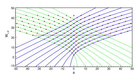
Figure 1: Eigenvalues $W_{0}^{(n)}$ ($b=0$) from the truncation condition (red points) and $W_{\nu,0}(a)$ (blue, continuous lines) and $W_{\nu,0}(-a)$ (green, dashed lines) obtained by means of the variational method

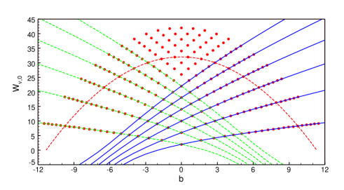
Figure 2: Eigenvalues $W_{0}^{(n,i)}$ ($a=0$) from the truncation condition (red points) and $W_{\nu,0}(b)$ (blue, continuous lines) and $W_{\nu,0}(-b)$ (green, dashed lines) obtained by means of the variational method

References

- [1] Verçin A 1991 Phys. Lett. B 260 120.
- [2] Myrheim J, Halvorsen E, and Verçin A 1992 Phys. Lett. B 278 171.
- [3] Taut M 1993 Phys. Rev. A 48 3561.
- [4] Taut M 1994 J. Phys. A 27 1045.
- [5] Taut M 1995 J. Phys. A 28 2081.
- [6] Furtado C, da Cunha B G C, Moraes F, Bezerra de Mello E R, and Bezzerra V B 1994 Phys. Lett. A 195 90.
- [7] Bakke K and Moraes F 2012 Phys. Lett. A 376 2838.
- [8] A. L. Cavalcanti de Oliveira and E. R. Bezerra de Mello, Exact solutions of the Klein-Gordon equation in the presence of a dyon, magnetic flux and scalar potential in the spacetime of gravitational defects, Class. Quantum Grav. 23 (2006) 5249-5263.
- [9] Figueiredo Medeiros E R and Bezerra de Mello E R 2012 Eur. Phys. J. C 72 2051.
- [10] Bakke K and Belich H 2012 Eur. Phys. J. Plus 127 102.
- [11] Bakke K and Belich H 2013 Ann. Phys. (Berlin) 526 187.
- [12] Bakke K 2014 Ann. Phys. 341 86.
- [13] Bakke K 2014 Int. J. Mod. Phys. A 29 1450117.
- [14] Bakke K and Belich H 2014 Eur. Phys. J. Plus 129 147.
- [15] Fonseca I C and Bakke K 2015 J. Math. Phys. 56 062107.
- [16] Bakke K and Furtado C 2015 Ann. Phys. 355 48.
- [17] A. S. Oliveira and K. Bakke, Effcts on a Landau-type system for a neutral particle with no permanent electric dipole moment subject to the Kratzer potential in a rotating frame, Proc. Roy. Soc. A 472 (2016) 20150858.
- [18] Vitória L L, Bakke K, and Belich H 2018 Ann. Phys. 399 117.
- [19] Vitória L L, Furtado C, and Bakke K 2018 Eur. Phys. J. C 78 44.
- [20] Vitória L L and Bakke K 2018 Int. J. Mod. Phys. D 27 1850005.
- [21] Bakke K and Salvador C 2018 Proc. Roy. Soc. A 474 20170881.
- [22] Vitória L L and Belich H 2019 Phys. Scr. 94 125301.
- [23] Bakke K, Ribeiro R F, and Salvador C 2019 Int. J. Mod. Phys. A 34 1950229.
- [24] Oliveira A S, Maluf R V, and Almeida C A S 2019 Ann. Phys. 400 1.
- [25] Leite E V B, Vitória L L, and Belich H 2019 Mod. Phys. Lett. A 34 1950319.
- [26] Vieira S L R and Bakke K 2020 Phys. Rev. A 101 032102.
- [27] Vitória L L and Belich H 2020 Eur. Phys. J. Plus 135 247.
- [28] Oliveira A S, Bakke K, and Belich H 2020 Eur. Phys. J. Plus 135 623.
- [29] Hassanabadi H, de Montigny M, and Hosseinpour M 2020 Ann. Phys. 412 168040.
- [30] Ahmed F 2020 Eur. Phys. J. C 80 211.
- [31] Ahmed F 2020 Eur. Phys. J. Plus 135 588.
- [32] Ahmed F 2021 Mod. Phys. Lett. A 36 2150004.
- [33] Fernández F M 2020 Dimensionless equations in non-relativistic quantum mechanics. arXiv:2005.05377 [quant-ph]
- [34] Güttinger P 1932 Z. Phys. 73 169.
- [35] Feynman R P 1939 Phys. Rev. 56 340.
- [36] Bera S, Chakrabarti B, and Das T K 2017 Phys. Lett. A 381 1356.
- [37] Turbiner A V 2016 Phys. Rep. 642 1. arXiv:1603.02992 [quant-ph].
- [38] Child M S, Dong S-H, and Wang X-G 2000 J. Phys. A 33 5653.
- [39] Amore P and Fernández F M 2020 Phys. Scr. 95 105201. arXiv:2007.03448 [quant-ph]
- [40] Pilar F L 1968 Elementary Quantum Chemistry (McGraw-Hill, New York).
- [41] P. Amore and F. M. Fernández, An ubiquitous three-term recurrence relation, J. Math. Phys. 62 (2021) 032106.