The TRAPPIST-1 Habitable Atmosphere Intercomparison (THAI).
Part III: Simulated Observables – The return of the spectrum

Abstract

The TRAPPIST-1 Habitable Atmosphere Intercomparison (THAI) is a community project that aims to quantify how differences in general circulation models (GCMs) could impact the climate prediction for TRAPPIST-1e and, subsequently its atmospheric characterization in transit. Four GCMs have participated in THAI: ExoCAM, LMD-Generic, ROCKE-3D and the UM. This paper, focused on the simulated observations, is the third part of a trilogy, following the analysis of two land planet scenarios (Part I) and two aquaplanet scenarios (Part II). Here, we show a robust agreement between the simulated spectra and the number of transits estimated to detect the land planet atmospheres. For the aquaplanet ones,a 5–$\sigma$ detection of CO₂ could be achieved in about 10 transits if the atmosphere contains at least 1 bar of CO₂. That number can vary by 41–56$\%$ depending on the GCM used to predict the terminator profiles, principally due to differences in the cloud deck altitude, with ExoCAM and LMD-G producing higher clouds than ROCKE-3D and UM. for the first time, this work provides “GCM uncertainty error bars” of $\sim 50\%$ that need to be considered in future analyses of transmission spectra. We also analyzed the inter-transit variability . Its magnitude differs significantly between the GCMs but its impact on the transmission spectra is within the measurement uncertainties. THAI has demonstrated the importance of model intercomparison for exoplanets and also paved the way for a larger project to develop an intercomparison meta-framework, namely the Climates Using Interactive Suites of Intercomparisons Nested for Exoplanet Studies (CUISINES).

1 Introduction

Here at last… comes the end of our fellowship. I will not say do not weep, for not all tears are an evil.

—J.R.R. Tolkien, The Return of the King

At the dawn of terrestrial exoplanet atmospheric characterization with the James Webb Space Telescope (JWST), predicting the detectability of the atmospheres of such planets is crucial in order to prepare for observations and maximize the scientific return. JWST Guaranteed Time Observations (GTO) and Cycle 1 proposals have already been selected. While CO₂ can be potentially detectable from Cycle 1, it is unlikely that enough transits would be accumulated for any single target to characterize the atmosphere of a terrestrial exoplanet (Fauchez et al., 2019; Lustig-Yaeger et al., 2019; Pidhorodetska et al., 2020) in the Habitable Zone (HZ; see e.g. Kopparapu et al., 2013) of M–dwarf stars. The presence of CO₂ has been shown to be the best proxy (Fauchez et al., 2019; Lustig-Yaeger et al., 2019; Turbet et al., 2020) for the detection of a potentially habitable atmosphere due to its strong absorption band in the mid-infrared (MIR) at 4.3 $\mu m$ and in the far-infrared at $\sim$ 15 $\mu m$. However a 5–$\sigma$ detection under cloudy conditions would likely require more than a dozen transits, even for the most favorable HZ terrestrial planet, TRAPPIST-1e (Fauchez et al., 2019).

TRAPPIST-1e belongs to the seven small transiting planet system TRAPPIST-1 (Gillon et al., 2016, 2017; Luger et al., 2017) at 12.0 pc away. The star, TRAPPIST-1, is a M8V just slightly larger than Jupiter which makes it very suitable for transmission spectroscopy of the atmosphere of small rocky planets. Indeed, the ratio of the surface area of the star’s disk blocked out by the planet’s disk (including its atmosphere), i.e. the transit depth, is inversely proportional to the square of the star radius. Also, around such cold and dim star HZ planets have a very short orbital period leading to very frequent transits and therefore more accessible data on their atmospheres. The Hubble Space Telescope (HST) has been used to infer the presence of an atmosphere on TRAPPIST-1e and its sibling planets (de Wit et al., 2016, 2018). However, the precision of HST data were only able to rule out clear–sky H₂ dominated atmospheres while Moran et al. (2018) showed that HST observations could actually be fit by cloudy/hazy H₂ atmospheres. Yet, TRAPPIST-1e bulk density measurements (Grimm et al., 2018; Agol et al., 2021) to H₂-rich planets mass-radius relationships (Turbet et al., 2020) along with atmospheric escape modelling and gas accretion modelling (Hori & Ogihara, 2020) provide accumulating evidence against the presence of H₂ dominated cloudy atmospheres around TRAPPIST-1 planets, including TRAPPIST-1e (see Turbet et al. 2020 and references therein). Furthermore, Krishnamurthy et al. (2021) reported strong upper limit constraints on the absence of helium in the atmosphere of TRAPPIST-1e. More in-depth knowledge about the absence or presence of a high mean molecular weight atmosphere on TRAPPIST-1e would most likely require JWST transit observations. Indeed, even some of the largest planned optical telescope (Extremely Large Telescopes, ELTs) are unable — even at the diffraction limit — to separate the light from TRAPPIST-1 and its planets, because of their very small angular separation. The same is true for future space observatories such as the Roman (Douglas et al., 2020), Large UV/Optical/Infrared Surveyor (LUVOIR, Team (2019)), the Habitable Exoplanet Observatory HabEx (Gaudi et al. (2018)) for which the inner working angle of their coronagraph would block the light not only from the star but from the entire system. Also, in the HZ, the planet is relatively too cold to significantly emit thermal infrared radiation which makes it very challenging to characterize its emission spectrum (Fauchez et al., 2019; Lustig-Yaeger et al., 2019; Kane et al., 2021); more close-in planets, however, will be more sensitive to this technique (Morley et al., 2017; Lustig-Yaeger et al., 2019; Koll et al., 2019; Turbet et al., 2020). Orbital broadband phase-dependent variations in the combined planetary thermal emission and reflected stellar energy can also provide clues about the atmospheric structure and surface properties of the planet (e.g. Selsis et al., 2011; von Paris et al., 2016; Koll & Abbot, 2016; Turbet et al., 2016; Haqq-Misra et al., 2018; Wolf et al., 2019), but the level of the phase variation of part-per-billion (ppb) are far beyond our current instrumental capabilities (Wolf et al., 2019). Atmospheric characterization of TRAPPIST-1e may be also possible from the ground (Wunderlich et al., 2020) with the planned European Extremely Large Telescope (E-ELT), but this demonstration has been done assuming a clear-sky TRAPPIST-1e atmosphere, which may have led to an over-estimation of the E-ELT’s capabilities.

Therefore, JWST transit observations are the most viable atmospheric characterization technique for the TRAPPIST-1 planets in the coming decade. Several studies have used either GCMs (Fauchez et al., 2019; Pidhorodetska et al., 2020; May et al., 2021) or 1-D radiative convective climate models coupled to photochemistry (Lincowski et al., 2018; Lustig-Yaeger et al., 2019; Wunderlich et al., 2019, 2020; Lin et al., 2021) or analytical models (Morley et al., 2017) to predict the detectability of standard atmospheres such as the modern Earth, the Archean Earth or a CO₂-dominated atmosphere. While these predictions inherently vary from one model category to another due to for instance the day/night contrast or the presence of clouds and hazes in the simulated atmosphere, models in the same category may also disagree due to, for example, differences in the atmospheric profiles at the terminator. Evaluating these differences and their impact on synthetic observations in order to optimize JWST observation strategies are the core objectives of the TRAPPIST-1 Habitable Atmosphere Intercomparison (THAI; Fauchez et al., 2020a, 2021). The comparison of these simulated climate systems are described in the companion papers (Turbet et al., 2021, referred to as Part I) for the dry planet benchmark scenarios (Ben 1 & Ben 2) and in (Sergeev et al., 2021, referred to as Part II) for the aquaplanet (Hab 1 & Hab 2) scenarios. The paper is structured as follows: In Section 2 the methods and tools used in his study are described. In Section 3, we present the simulated transmission spectra using each of the GCM outputs, using both time average and time dependent terminator profiles. Finally, conclusions are given in Section 4.

2 Method

2.1 The THAI GCM simulations

In this paper, Part III of a trilogy of THAI papers, we use the same GCM simulations that have been extensively analyzed in Part I (Turbet et al., 2021) and Part II (Sergeev et al., 2021), namely the Ben 1 & Ben 2 and Hab 1 & Hab 2 cases, respectively. Briefly, the Ben 1 & Ben 2 cases are dry land planet simulations, while the Hab 1 & Hab 2 cases assume that the surface is fully covered by a global (static) ocean and that there is water vapour and clouds in the atmosphere. Ben 1 & Hab 1 atmospheric composition is broadly similar to that of modern Earth (1 bar of N₂, 400 ppmv of CO₂), while the Ben 2 & Hab 2 experiments assume a CO₂-dominated atmosphere (1 bar). 10 orbits (61 Earth days) at a frequency of 6 h are output for Ben 1 & Ben 2, while 100 orbits (610 Earth days) are output for Hab 1 & Hab 2, in order to smooth out the internal variability with a period of about a dozen of orbits induced by clouds.

Each of these simulations have been performed by the four THAI GCMs: ExoCAM (Wolf et al., 2022) the exoplanet branch of the Community Earth System Model (CESM, http://www.cesm.ucar.edu/models/cesm1.2/) version 1.2.1., the LMD Generic model (LMD-G, see e.g. Wordsworth et al., 2011; Turbet et al., 2018), the Resolving Orbital and Climate Keys of Earth and Extraterrestrial Environments with Dynamics (ROCKE-3D Way et al., 2017)) and the Met Office Unified Model (the UM, see e.g. Mayne et al., 2014; Boutle et al., 2017). More details on these four GCMs are also provided in the THAI protocol (Turbet et al., 2021; Sergeev et al., 2021) and the THAI workshop report (Fauchez et al., 2021).

2.2 Simulated Spectra

We use the Planetary Spectrum Generator (PSG, Villanueva et al., 2018, 2022) to simulate transmission spectra of TRAPPIST-1e for each of the THAI scenarios, using data from each of the four GCMs. PSG is an online radiative transfer tool that can be used to simulate planetary spectra observations from any ground or space-based observatory for various objects of the solar system and beyond, and it also includes a noise calculator.

To simulate and compare time-averaged transmission spectra across the models, we first average the atmospheric properties over the 10 orbits of Ben 1 & Ben 2 and over the 100 orbits of Hab 1 & Hab 2. For our transit calculations, atmospheric profiles were created for each GCM latitude $\times$ longitude cell at the terminator of the planet using abundance, pressures, temperatures as reported by the GCM for that specific terminator cell (vertical parameters of that cell). Then transit spectra were computed using those profiles across all terminator cells, and the total transit spectrum was computed by the average of all transits across the terminators (weighted by the latitudinal extension of the cell).

Specifically, the radiative transfer is computed employing a layer-by-layer pseudo-spherical refractive raytracing algorithm. Rayleigh cross-sections are computed as a summation of the individual molecular cross-sections (Villanueva et al., 2022; Sneep & Ubachs, 2005), which are computed at each wavelength based on the polarizability of the encompassing molecules. PSG employs polarizability values as compiled on the Computational Chemistry Comparison and Benchmark DataBase at NIST (https://cccbdb.nist.gov/pollistx.asp). Collision-induced absorptions (CIA) generated by inelastic collisions of molecules in a gas are included from considering the latest HITRAN CIA compilations (Gordon et al., 2022) and and the HITRAN CIA database (Karman et al., 2019), as well as several other sources as reported in (Villanueva et al., 2022), including the MT_CKD water continuum (Mlawer et al., 2012), here in version v3.5 (Payne et al., 2020; Kofman & Villanueva, 2021)). In the presented spectral range and assumed background abundance, only these CIAs contain notable signatures: CO₂–CO₂, H₂O–H₂O, H₂O–N₂, N₂–N₂. Molecular absorptions were included via correlated-k tables based on the latest HITRAN 2020 linelist (Gordon et al., 2022), which were complemented at short wavelengths ($<1$ $\mu m$) with UV cross-sections, primarily from the MPI Mainz UV/VIS Spectral Atlas (Keller-Rudek et al., 2013). Aerosols properties are modelled following Mie theory, with water cloud scattering properties as described in Massie & Hervig (2013) while the ice cloud optical property parameterization uses Warren (1984), as also described in Massie & Hervig (2013). The partial abundance of the aerosols at the grid-box is explicitly defined by the GCM kg/kg profile at that location, meaning that a profile with zero abundance would correspond to a fully clear scenario. An average of all these spectra is then computed to obtain a limb-averaged spectra as it would be observed by an instrument.

2.3 Instruments, noise and number of transits

2.3.1 Instruments

We have simulated JWST observations of TRAPPIST-1e transiting its host star. JWST is a 6.5 m tip-to-tip segmented telescope, equivalent to a full circular aperture of 5.6 m of diameter. Previous studies have showed that the NIRSpec Prism (covering the $0.6-5.3~{}\mu m$ region at resolving power R=100) is the JWST instrument most adapted to characterize the atmosphere of temperate terrestrial planets (Fauchez et al., 2019; Lustig-Yaeger et al., 2019; Pidhorodetska et al., 2020; Wunderlich et al., 2020). Indeed, this spectral region contains various molecular signatures of interest such as O₂, H₂O, NO₂, N₂O, CH₄, CO and CO₂. The latter may likely be the only one with a strong enough absorption features to be detectable with JWST in a reasonable number of transits , when clouds and hazes are present in the atmosphere. It has therefore been suggested as the best proxy to detect the atmosphere of habitable planets (Fauchez et al., 2019; Turbet et al., 2020). Note that JWST Guaranteed Time Observations (GTO) proposals have already been awarded for the NIRSpec instrument that will attempt molecular detection . In this work we compute spectra from 0.6 to 20 $\mu m$, across the range of both JWST NIRSpec Prism and MIRI medium-resolution spectrometer (MRS) and present the figures at R=100 offering the best visibility for multiple spectrum plots. .

2.3.2 Noise

2.3.3 Estimation of the detectability of the atmosphere — identical transits

we computed noise estimates with PSG, and validated these by employing the official JWST Exposure Time Calculator, obtaining very good agreement. For NIRSpec Prism, the effective spectral resolution is 0.022 $\mu m$. We have selected the clear filter with the sub–array SUB512S and the rapid readout pattern with two groups per integration and 0.225 s per frame. This leads to a partial saturation near the peak of the Stellar Energy Distribution (SED) following (Batalha et al., 2018; Lustig-Yaeger et al., 2019). For MIRI LRS, the effective resolution is 0.0654  $\mu m$, and we selected the P750L disperser with the sub–array SLITLESSPRISM, and a FASTR1 readout pattern with 20 groups per integration with a frame time of 0.15 s.

$$N =\sqrt{N_{out}^{2}+N_{in}^{2}}$$ (1)

$$=\sqrt{(1/time_{out})^{2}+(1/time_{in})^{2}}$$

$$=\sqrt{(1/3)^{2}+(1/1)^{2}}$$

$$=\sqrt{4/3}$$

To estimate the 1 transit S/N of CO₂ across the NIRSpec Prism range (0.6-5.3 $\mu m$) and the number of transits required to achieve a 5–$\sigma$ detection of CO₂ we proceed following the list below:

1. We compute the spectrum without CO₂ (but keeping the other gases in)

2. We compute the spectrum with CO₂

3. We compute the difference between step 1. and 2 across the whole instrument range

4. We compute the S/N by dividing step 3. by the noise for 1 transit (3345 s) in each spectral interval.

5. We apply the $\sqrt{4/3}=1.155$ factor to the noise to take into account the out-of-transit noise.

6. The S/N of CO₂ across the whole instrument range then computed following Lustig-Yaeger et al. (2019) as:

   $$S/N=\sqrt{\sum_{i=0}^{n}S/Ni^{2}},$$ (2)

   where S/Ni are the individual S/N in each spectral interval.

7. From the S/N, the number of transits $N_{t}$ required to achieve a 5–$\sigma$ detection is done as following Fauchez et al. (2019, 2020b):

   $$N_{t}=\left(\frac{5}{S/N}\right)^{2}.$$ (3)

3 Transmission Spectra

3.1 Ben 1 & Ben 2 cases (dry planets)

In Fig. 1 and 2 we can see the transmission spectra simulated with PSG using the atmospheric profiles of THAI cases Ben 1 & Ben 2, respectively, provided by each GCM. In the panel A) of both figures, the lowest pressures (highest altitudes) used to compute the spectra correspond to the top of the modelled domains, which are 10^-5, 4$\times$10^-5, 14$\times$10^-5 and 4$\times$10^-5 bar for Ben 1 and 10^-5, 4$\times$10^-5, 14$\times$10^-5 and 13$\times$10^-5 bar for Ben 2 for ExoCAM, LMD-G, ROCKE-3D and the UM, respectively. Note that most GCMs have the domain lid at relatively high pressures for numerical stability reasons and as moving it to lower pressures require taking into account complex upper atmospheric processes such as non-local thermodynamic equilibrium, molecular diffusion, etc (see Fauchez et al. (2021), section 4.1). The lowest pressures usually correspond to a top-of-atmosphere (TOA) altitude of 50 to 70 km for Earth-like simulations. However, the pressure at this altitude is usually too high to fully capture the transmitted light through the planet’s atmosphere and the strongest atmospheric features can be truncated. This is clearly seen in the Ben 2 case where the CO₂ strongest absorption lines are truncated (Fig. 2a). To bypass this limitation, we used PSG to extend the atmosphere to much lower pressures, assuming an isothermal profile and constant volume mixing ratios for the dry gases. This is similar to the so-called “ghost layer” used in Amundsen et al. (2016). We have estimated the TOA pressure that would fully resolve the spectral lines for Ben 1 & Ben 2 as 10^-7 and 10^-10 bar, respectively. Lower pressures are required for Ben 2 because the opacity of a pure CO₂ atmosphere remains strong at lower pressures than that of a N₂-dominated atmosphere.

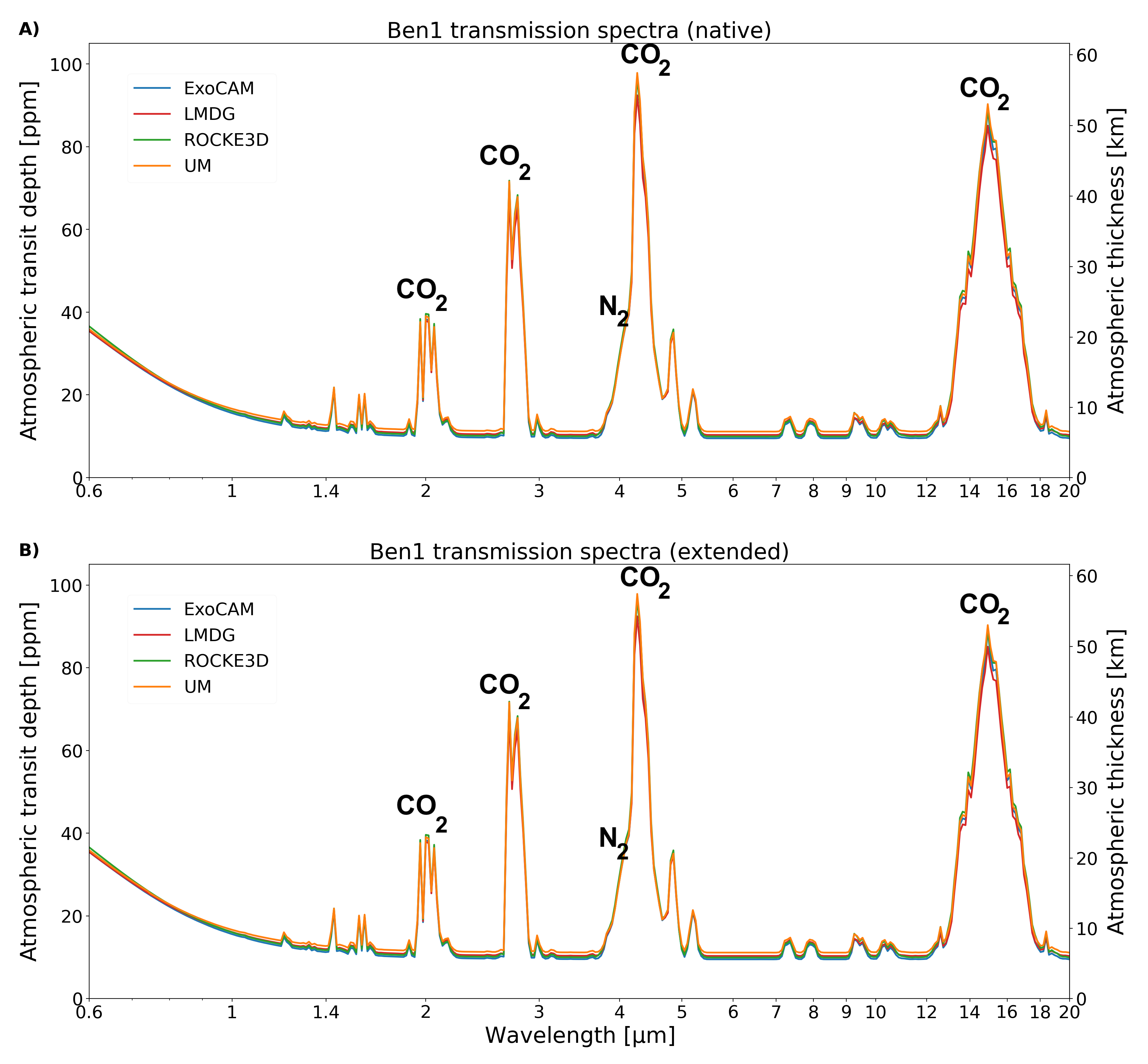
Figure 1: Ben 1 transmission spectra simulated with PSG using the terminator atmospheric profiles from the ExoCAM, LMD-G, ROCKE-3D and the UM simulations. In Panel A) the atmospheric profiles are limited up to the lowest pressure at the top of the GCMs, namely 10^-5, 4$\times$10^-5, 14$\times$10^-5 and 4$\times$10^-5 bar for ExoCAM, LMD-G, ROCKE-3D and UM, respectively while in Panel B) the atmospheric profiles have been extended up to 10^-7 bar assuming an isothermal atmosphere and fixed mixing ratios for the dry gases. The differences between the transmission spectra are extremely small.

Using the data with extrapolated model top, we have estimated the number of transits that would be required to detect such atmospheres with a 5–$\sigma$ confidence level

First, we can see that for a Ben 1 atmosphere, an average of $2.6~{}\sigma$ could be achieved from Cycle 1 while an average of $4.3~{}\sigma$ could be achieved for a Ben 2 atmosphere with more CO₂. To reach the necessary 5–$\sigma$ threshold, an average of 17 and 6 transits would be needed for Ben 1 and Ben 2, respectively. When using only the CO₂ line at 4.3$\mu m$ these numbers go up to 24 and 25 transits, respectively. This demonstrates that this method strongly over-estimates the number of necessary transits, especially if the amount of CO₂, and therefore the number of strong lines, is high. The inter-model differences are small in both cases demonstrating that the four GCMs provide similar atmospheric profiles at the terminator to provide consistent simulated spectra and expected number of transits to detect a dry 1 bar atmosphere with a relatively high mean molecular weight. Note that we did not consider the spectral impact of dust that can be lifted from the surface of a land planet and persist in the atmosphere. Dust would likely raise the continuum level, thereby decreasing the amplitude of each spectral line as shown in Boutle et al. (2020). The expected effect would be of the order of 10 ppm.

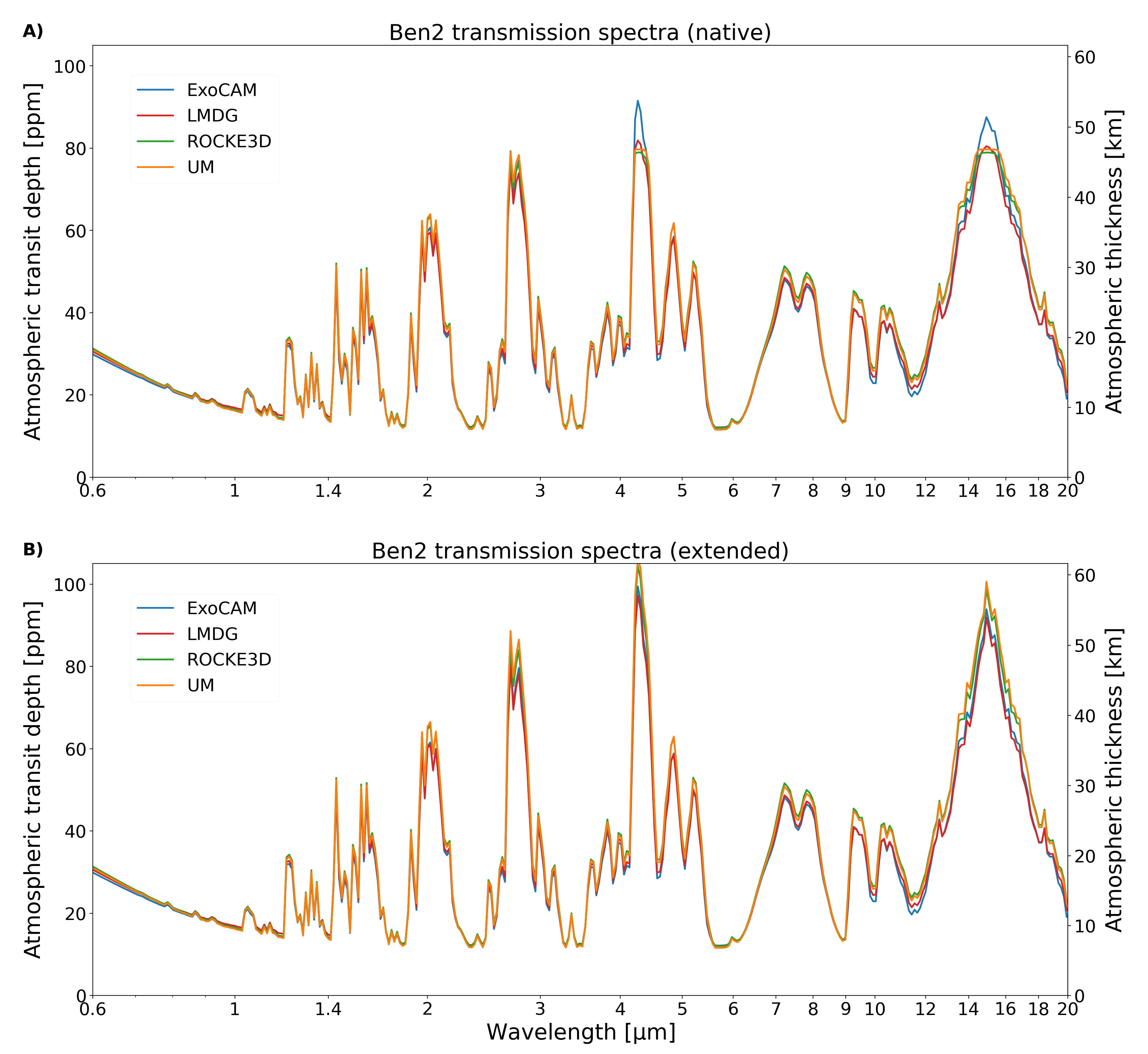
Figure 2: Ben 2 transmission spectra simulated with PSG using the terminator atmospheric profiles from the ExoCAM, LMD-G, ROCKE-3D and UM simulations. In Panel A) the atmospheric profiles are limited up to the lowest pressure at the top of the GCMs, namely 10^-5, 4$\times$10^-5, 14$\times$10^-5 and 13$\times$10^-5 bar for ExoCAM, LMD-G, ROCKE-3D and the UM, respectively while in Panel B) the atmospheric profiles have been extended up to 10^-10 bar assuming an isothermal atmosphere and fixed mixing ratios for the dry gases. CO₂ features are truncated if the atmospheres are not vertically extended. Visible differences between the spectra appear in the CO₂ bands in both the native (panel A) and extended (panel B) scenarios.

Table 1: Table summarizing the signal-to-noise ratio achieved from 1 transit (S/N-1), from the four JWST Cycle 1 transits (S/N-4), number of transits to reach a 5–$\sigma$ detection using all available CO₂ lines (5–$\sigma$ Transit), and using only the 4.3 $\mu m$ CO₂ line.

	Ben1
Model	S/N-1	S/N-4	5–$\sigma$ Transit	5–$\sigma$ Transit-4.3$\mu m$
ExoCAM	1.3	2.6	16	23
LMD-G	1.2	2.4	19	25
ROCKE-3D	1.3	2.6	15	23
UM	1.3	2.6	16	23
Average	1.3	2.6	17	24
Maximum difference (%)	8	8	24	8
	Ben2
Model	S/N-1	S/N-4	5–$\sigma$ Transit	5–$\sigma$ Transit-4.3$\mu m$
ExoCAM	2.2	4.4	5	23
LMD-G	2.0	4.0	7	28
ROCKE-3D	2.2	4.4	5	23
UM	2.2	4.4	5	24
Average	2.2	4.3	6	25
Maximum difference (%)	9	9	33	20
	Hab1
Model	S/N-1	S/N-4	5–$\sigma$ Transit	5–$\sigma$ Transit-4.3$\mu m$
ExoCAM	0.9	1.8	35	39
LMD-G	0.9	1.8	29	37
ROCKE-3D	1.0	2.0	38	31
UM	1.0	2.0	23	24
Average	1.0	2.0	29	33
Maximum difference (%)	10	10	41	45
	Hab2
Model	S/N-1	S/N-4	5–$\sigma$ Transit	5–$\sigma$ Transit-4.3$\mu m$
ExoCAM	1.5	3.0	12	36
LMD-G	1.7	3.4	9	31
ROCKE-3D	1.7	3.4	8	29
UM	2.0	4.0	7	23
Average	1.7	3.4	9	30
Maximum difference (%)	29	29	56	43

3.2 Hab 1 & Hab 2 cases (aquaplanets)

Rocky exoplanets in the HZ and with surface liquid water will likely have water in a vapor and condensed form in the atmosphere. Clouds have been shown to severely impede atmospheric characterization via transmission spectroscopy (Fauchez et al., 2019; Komacek et al., 2020; Suissa et al., 2020a). Furthermore, clouds are notoriously difficult to represent correctly in GCMs, because the characteristic timescale and size of individual clouds is too small to be simulated explicitly and they involve a tremendous amount of physical processes. GCMs thus rely on sub-grid scale parameterizations to represent the formation of clouds that can significantly differ between models (Sergeev et al., 2021). These discrepancies can then lead to different predicted surface temperatures, as was noted in exoplanet GCM simulations by Yang et al. (2019). Details on the differences in GCM predictions, especially for clouds, are given in the companion paper (Sergeev et al., 2021).
Here, we use PSG to compute transmission spectra for both the Hab 1 & Hab 2 cases. The atmospheric properties at the terminator have been time averaged over the 100 orbits in order to smooth out variability that can be introduced by weather patterns and change in clouds at the terminator, as is commonly done for such planets (Fauchez et al., 2019; Komacek et al., 2020; Pidhorodetska et al., 2020; Suissa et al., 2020a, b). Details on the impact of atmospheric variability on transmission spectra are given in Sec. 3.3.

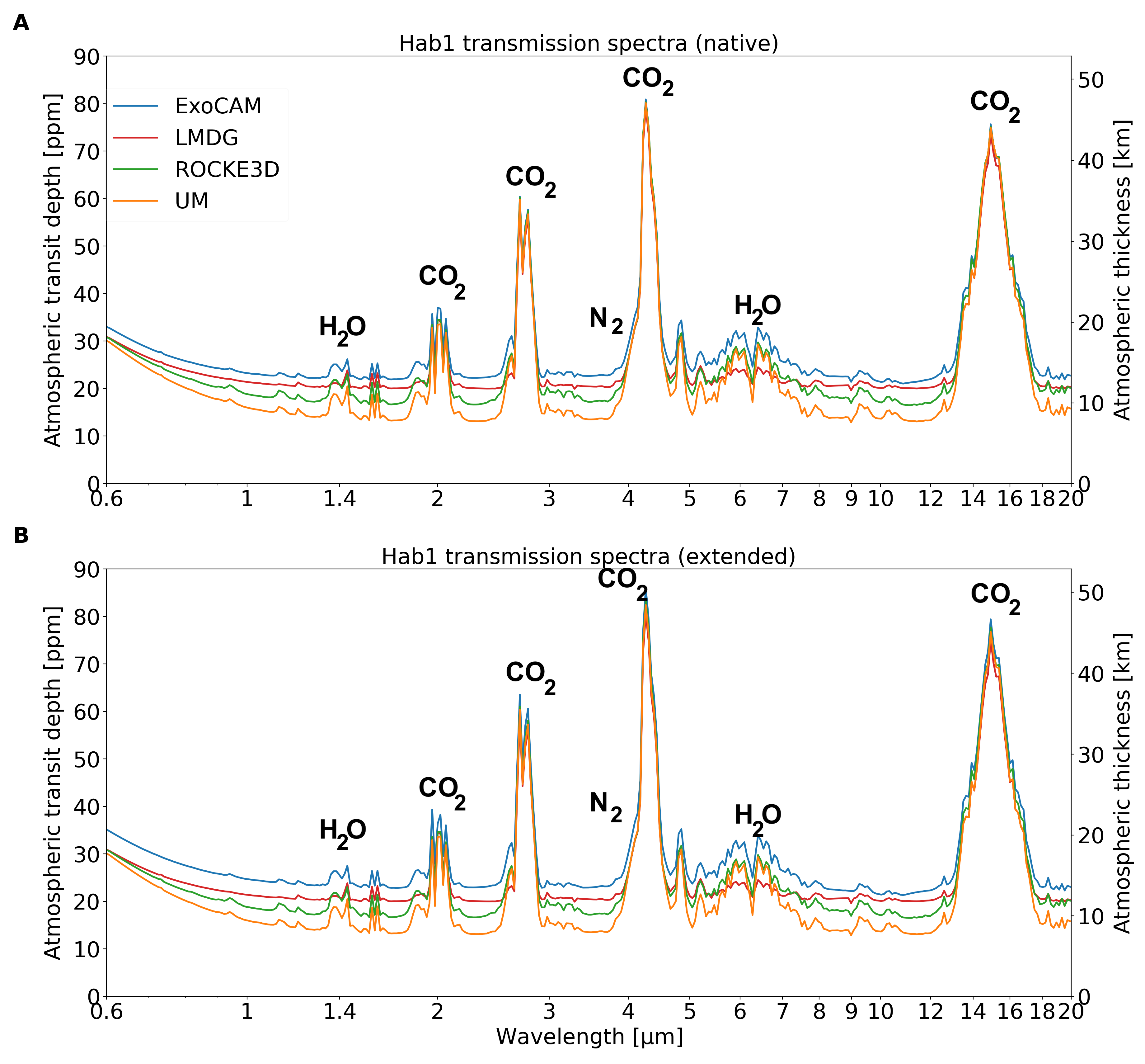
Figure 3: Hab 1 transmission spectra simulated with PSG using the terminator atmospheric profiles from the ExoCAM, LMD-G, ROCKE-3D and the UM simulations. In Panel A) the atmospheric profiles are limited up to the lowest pressure a the top of the GCMs, namely 10^-5, 4$\times$10^-5, 14$\times$10^-5 and 4$\times$10^-5 bar for ExoCAM, LMD-G, ROCKE-3D and the UM, respectively while in Panel B) the atmospheric profiles have been extended up to 10^-7 bar assuming an isothermal atmosphere and fixed mixing ratios for the dry gases.

Fig. 3 shows the Hab 1 transmission spectra calculated using the output from ExoCAM, LMD-G, ROCKE-3D and the UM. The extension of the top of the model has a negligible impact on the spectra, except within the strongest 4.3 $\mu m$ and 15 $\mu m$ CO₂ absorption bands. The differences between the spectra from the different GCMs are mostly noticeable in the continuum and for the weakest absorption bands. Indeed, as already shown by Fauchez et al. (2019) and Suissa et al. (2020a), the continuum level in a cloudy atmosphere is raised to the altitude of the cloud deck. Strong bands like CO₂ at 4.3 $\mu m$ are less affected by clouds because even if the denser, most absorbing part of the atmosphere is under them, the efficiency of absorption is so strong that the small CO₂ partial pressure remaining above the cloud deck is large enough to saturate the line. The ExoCAM continuum level is the highest, followed by LMD-G, ROCKE-3D and the UM. This is explained by the fact that the liquid water cloud mixing ratio and the altitude of the cloud deck at the west and east terminators, respectively, are much higher in ExoCAM than in LMD-G, ROCKE-3D and the UM, in that order (Fig. 4e,f). Regarding ice clouds, while the mixing ratios predicted by each model are comparable, the average altitude of the clouds is different, with ExoCAM producing the highest ice clouds following by LMD-G, ROCKE-3D and UM (Fig. 4g,h).

Fig. 3 also shows that the LMD-G water band around 6 $\mu m$ is significantly weaker than that predicted by other models. This is due to the fact that LMD-G simulations have a much drier upper atmosphere (Fig. 4c,d) . The amount of water above the tropopause in LMD-G is primarily controlled by the tropopause temperature at the substellar point (where water is injected by deep moist convection) which is the coldest in LMD-G, especially at the western terminator (see the companion paper, Sergeev et al., 2021, Fig. 4). As a result, the detectability of water in Hab 1 simulations for LMD-G is even more challenging than for the other GCMs.

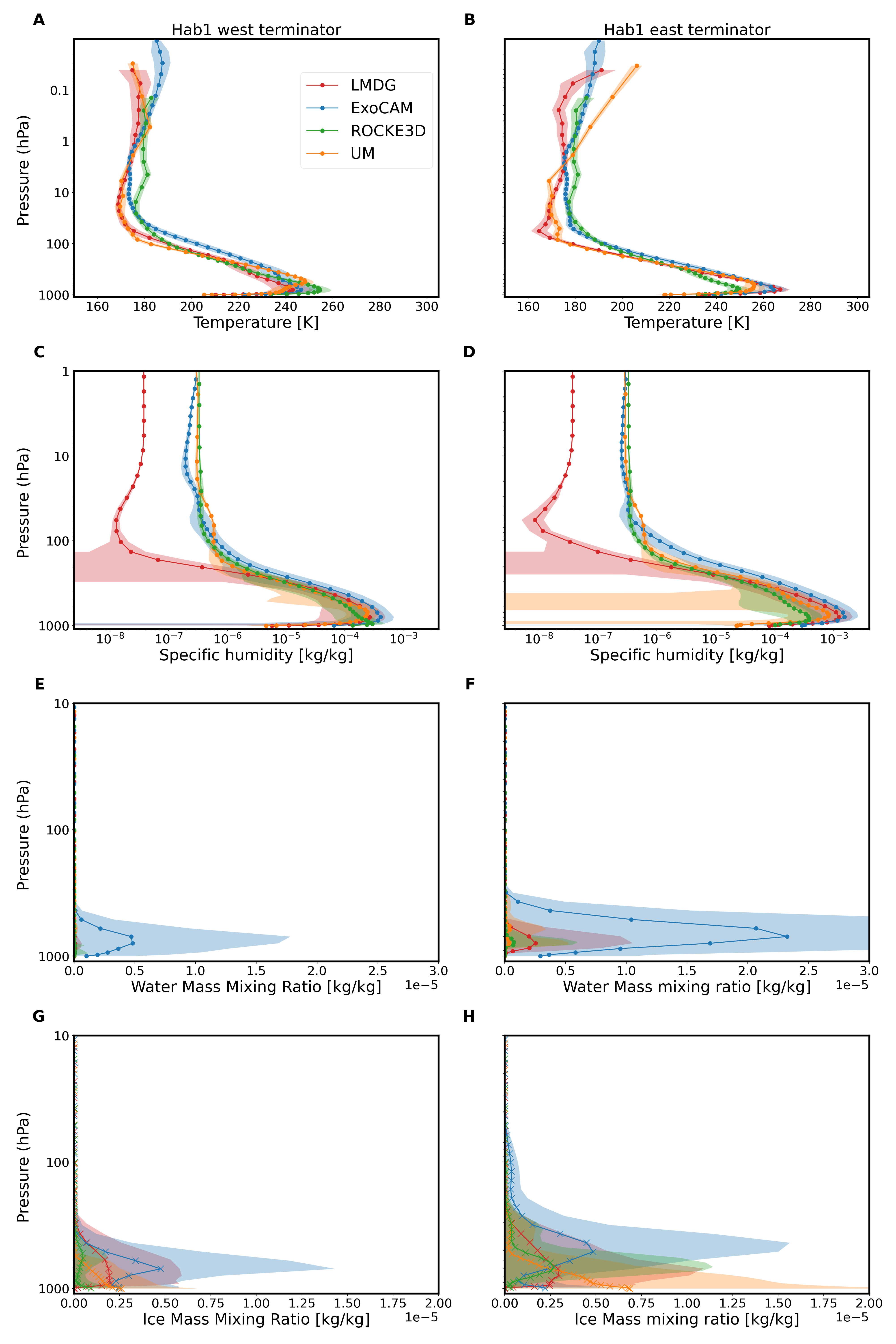
Figure 4: Hab 1 terminator atmospheric profiles predicted by ExoCAM (blue), LMD-G (red), ROCKE-3D (green) and the UM (orange). From top to bottom: temperature, specific humidity, the mass mixing ratio of liquid water and the mass mixing ratio of ice water for the west terminator (left column) and east terminator (right column). Time averaged values are represented by thick lines while the $1-\sigma$ deviations are represented by shades.

Figure 5: Hab 2 transmission spectra simulated with PSG using the terminator atmospheric profiles from the ExoCAM, LMD-G, ROCKE-3D and the UM simulations. In Panel A) the atmospheric profiles are limited up to the lowest pressure a the top of the GCMs, namely 10^-5, 4$\times$10^-5, 14$\times$10^-5 and 13$\times$10^-5 bar for ExoCAM, LMD-G, ROCKE-3D and UM, respectively while in Panel B) the atmospheric profiles have been extended up to 10^-10 bar assuming an isothermal atmosphere and fixed mixing ratios for the dry gases. CO₂ features are truncated if the atmospheres are not extended. Differences between the spectra due to clouds are mostly seen in the continuum and for the weakest absorption bands.

Fig. 5 is the same as Fig. 3, but for Hab 2 simulations. First, we can see that because the CO₂ mixing ratio is much higher in the Hab 2 simulations (from about 400 ppm for Hab 1 to nearly 100 $\%$ for Hab 2), strong absorption lines are more easily truncated by a low model top. Similarly to the Hab 1 case, the ExoCAM continuum is higher than that of the other three GCMs. This time, however, the continuum level in ROCKE-3D is slightly above that in LMD-G. Note that LMD-G’s absorption peaks are the smallest among the four GCMs.

In the warm and humid atmosphere of the Hab 2 case (Fig. 6a,b) there is no clear temperature inversion at the tropopause except for a decrease in the lapse rate from 100 hPa and lower (for more details see Sergeev et al., 2021). The specific humidity closely follows the temperature profiles: colder temperature profiles correspond to drier profiles (Fig. 6c,d). Furthermore, the warm atmosphere of Hab 2 results in the liquid water cloud mass mixing ratio being comparable and even larger than the ice cloud mixing ratio (Fig. 6). When the altitudes of both cloud types are combined, ExoCAM has on average higher and thicker clouds, followed by ROCKE-3D, then LMD-G and finally the UM. It is interesting to note that in the warmer, moister and cloudier Hab 2 case, the relative difference in cloudiness between LMD-G, ROCKE-3D and the UM is smaller than that for Hab 1. Only ExoCAM persistent produces higher clouds. More detailed discussion about the differences of cloud coverage produced by the THAI models are given in Sergeev et al. (2021).

Figure 6: Hab 2 terminator atmospheric profiles simulated by ExoCAM (blue), LMD-G (red), ROCKE-3D (green) and the UM (orange). From top to bottom: temperature, specific humidity, mass mixing ratio of liquid water and mass mixing ratio of ice water for the west terminator (left column) and east terminator (right column). Time averaged values are represented by thick lines while the 1–$\sigma$ deviations are represented by shades.

Similar to the Ben 1 & Ben 2 experiments, we extrapolated the model top for the PSG calculation, which gave the number of transits required for atmospheric detection with a 5–$\sigma$ confidence level by JWST using the CO₂ line at 4.3$~{}\mu m$ . For Hab 1, we found 35, 29, 38 and 23 transits are required, while for Hab 2 we found 12, 9, 8 and 7 transits are required (for ExoCAM, LMD-G, ROCKE-3D and UM, respectively).

The differences between the predicted transits is to the first order control by the altitude of the cloud deck and to the second order by the temperature profile. Those differences between ExoCAM and LMD-G on one hand and ROCKE-3D and the UM on the other are significant and could have consequences for the number of hours requested for a JWST proposal and on the interpretation of future data using retrieval algorithms. However, it seems clear that regardless the GCM used to produce the atmospheric data, at least 7 transit observations would be required to detect at a 5–$\sigma$ confidence level a high molecular weight atmosphere on TRAPPIST-1e with a cloudy sky.

Figure 7: Ben 1 (left column) and Hab 1 (right column) transmission spectra for ExoCAM (A and B panels), LMD-G (C and D panels), ROCKE-3D (E and F panels) and UM (G and H panels). The error bars are shown for the native NIRSpec spectral resolution and for 1 transit (green), 4 transits (magenta, NIRSpec Cycle 1 proposal 1331 (Lewis et al., 2017)), 20 transits (blue, $\sim$ 5 JWST years at a constant 4 transits per year) and 40 transits (red, $\sim$ 10 JWST years at a constant 4 transits per year). Relevant absorption features are written in white.

3.3 Inter-transit variability

Many previous modeling studies estimating the detectability of an exoplanet through transmission spectroscopy have assumed that each planetary transit will be constant through time (Fauchez et al., 2019; Lustig-Yaeger et al., 2019; Komacek et al., 2020; Pidhorodetska et al., 2020; Suissa et al., 2020a, b). However, this is not a realistic assumption as weather patterns and clouds, if present, are likely to change from one transit to another. Previous work on hot Jupiters by Komacek & Showman (2019) has shown that temporal variability could be already detectable using either secondary eclipse observations with JWST or phase curve observations, and/or Doppler wind speed measurements with high-resolution spectrographs. More recently, May et al. (2021) simulated TRAPPIST-1e with ExoCAM for various concentration of CO₂ and looked at the atmospheric variability between 10 transits induced by ice water clouds. The amplitude of the transit variability for their 10^-4 bar of CO₂ (comparable to Hab 1) and 1 bar CO₂ (comparable to Hab 2) are very similar, of the order of 10 and 20 ppm (May et al., 2021, their Fig. 4), respectively. However, they computed one transmission spectrum per day while in our study we compute it at the exact time of the transit, i.e. every 6.1 days, potentially leading to larger atmospheric differences. The main conclusion is that the time variability of the spectra does not affect retrieved abundances at detectable levels. However, the findings of May et al. (2021) are likely to be dependent on the GCM (ExoCAM). Here, we analyze the inter-transit variability produced by three more GCMs: LMD-G, ROCKE-3D and the UM.

Fig. 8 shows the standard deviation of the atmospheric transit depth and of the transit atmospheric thickness over 100 transits. This variability is wavelength dependent: it is the largest in the continuum as the transmitted light is closer to the surface, where clouds are present; and the smallest for the strongest absorption lines like the CO₂ at 2.7, 4.3 and 15 $\mu m$. There are significant differences between the GCMs. In general the cloudier the simulation is, the more variable the transmission spectrum is. For LMD-G and ROCKE-3D, the time variability in both Hab 1 and Hab 2 is remarkably similar, while for ExoCAM and the UM it differs. This difference is due to the change in the average altitude of clouds between Hab 1 ( 4) and Hab 2 ( 6). In LMD-G and ROCKE-3D simulations, the average altitude of liquid water and ice water clouds does not change substantially between Hab 1 and Hab 2, while for ExoCAM and the UM it increases sharply in Hab 2. For instance, for ExoCAM the east terminator water ice clouds maximum density peaks at 500 hPa for Hab 1 and at 250 hPa for Hab 2. We hypothesise that stronger winds at this lower pressure relative to those deeper in the atmosphere lead to higher cloud variability. Overall, the standard deviation of the continuum level in the Hab 1 case for ExoCAM, LMD-G, ROCKE-3D and the UM is about 3, 3, 2 and 1 ppm, respectively, leading to a median value of $\sim$2 ppm. For Hab 2 it is about 5, 3, 2.5 and 2 ppm, respectively, leading to a median value of $\sim$3 ppm. These values are low relative to the JWST expected 1–$\sigma$ noise of 10 to 25 ppm Fauchez et al. (2019) . It is also interesting to note that those values are comparable to the relative transit depth of H₂O or O₂ (Fauchez et al., 2019; Lustig-Yaeger et al., 2019; Pierrehumbert, 2010; Wunderlich et al., 2020). This means that even if one assume no noise floor, atmospheric variability would produce a continuum fluctuation that would swamp those highly important but weak absorption lines.

Figure 8: Standard deviation of the atmospheric transit depth [ppm] and of the atmospheric thickness [km] as a function of wavelength for Hab 1 (blue) and Hab 2 (red) and for ExoCAM (panel A), LMD-G (panel B), ROCKE-3D (panel C) and the UM (panel D).

Fig. 9 shows the spectra as the ratio in percentage of the standard deviation of the variability with respect to the measurement noise for 100 (blue), 50 (orange), 25 (green) and 10 (red) transits for the atmospheric transit depth (left Y axis) and atmospheric thickness (right Y axis). The larger the number of transits, the lower the noise and therefore the higher the variability-to-noise ratio (%). Interestingly, these spectra can be reminiscent of emission spectra (Morley et al., 2017; Lustig-Yaeger et al., 2019; Fauchez et al., 2019). The minimum values correspond to the absorption line peak, while the maxima correspond to the continuum. Only the Hab 2 atmosphere simulated by ExoCAM would lead to a transit depth and atmospheric thickness variability higher than the measurements noise if 100 transits or more are acquired with JWST. In a more realistic scenario of 50 non-consecutive transits accumulated over the lifetime of the JWST, the impact of atmospheric variability relative to the noise for Hab 1 and Hab 2 would be of about 50$\%$ and 80$\%$ for ExoCAM, 50$\%$ and 50$\%$ for LMD-G, 40$\%$ and 40$\%$ for ROCKE-3D and 20$\%$ and 40$\%$ for the UM, respectively, and will therefore be of a concern.

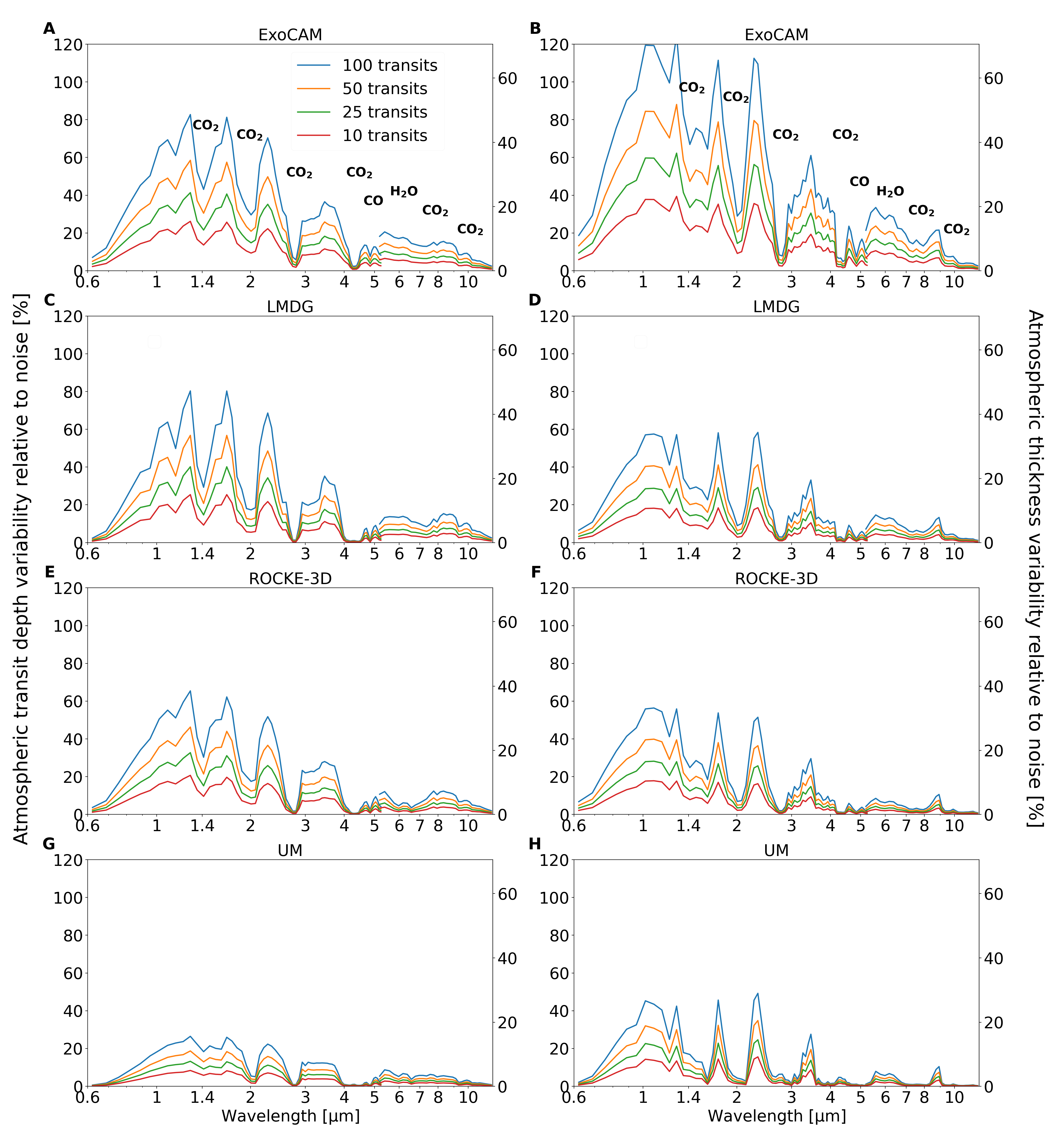
Figure 9: Atmospheric transit depth variability relative to noise (left Y axis) and atmospheric thickness variability relative to noise (right Y axis) for 100 (blue), 50 (orange), 25 (green) and 10 (red) transits for ExoCAM (panels A and B), LMD-G (panels C and D), ROCKE-3D (panels E and F) and the UM (panels G and H). Hab 1 is on the left column, Hab 2 on the right column. The noise is computed at the native instrument resolution and later binned down by a factor 3 for this figure.

Comparisons between all GCMs in a single panel is shown in Fig. 10. In panels A (Hab 1) and B (Hab 2) are shown each ExoCAM transmission spectrum (black lines) and the median spectrum (blue line) with the associated 1–sigma error (blue error bars). ExoCAM was selected for this example as it is the GCM showing the largest variability. In panels C (Hab 1) and D (Hab 2) the spectra of the variability relative to noise for 50 transits and for the four GCMs are shown.

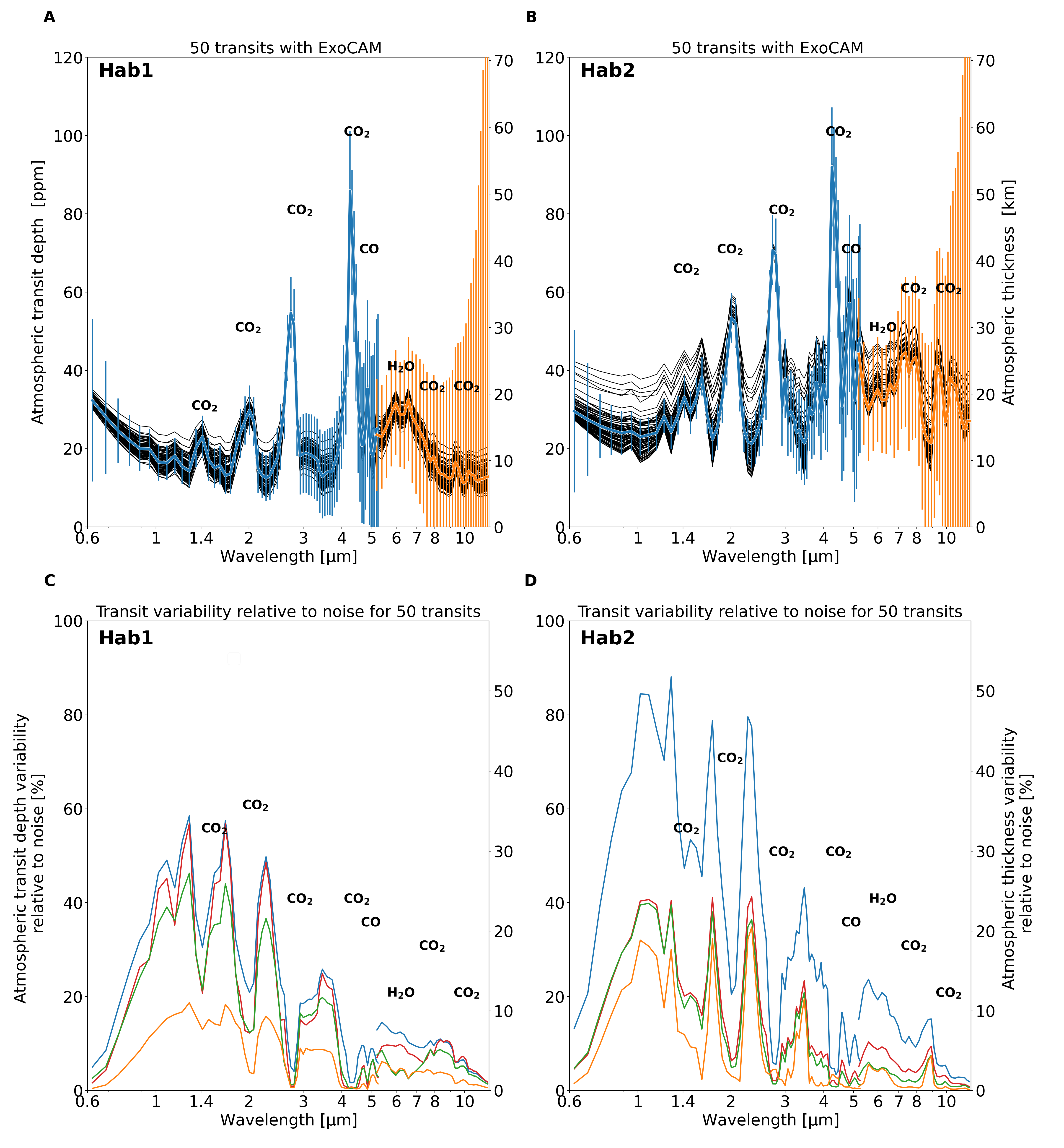
Figure 10: Panels A and B: transmission spectra for Hab 1 and Hab 2, respectively, obtained from ExoCAM simulations. Each fine black trace represents 1 of the 100 individual transits and the thick blue line represent the median transit. The noise for 50 transits and for both NIRSpec Prism (blue) and MIRI (orange) has been binned down by a factor 3 to maximize the number of photons per spectral bin while preserving the line shapes and is represented by the vertical error bars. Panels C and D: Hab 1 and Hab 2, respectively, atmospheric transit depth variability relative to noise (left Y axis) and atmospheric thickness variability relative to noise (right Y axis) for 50 transits and each of the four GCMs.

As a summary, in the case of TRAPPIST-1e it seems predictions of the atmospheric variability introduced by clouds for an N₂ or CO₂-dominated atmosphere are within the measurements noise for a reasonable number of transits ($<$ 50) regardless of the GCM used to simulate this temporal and spatial variability. However, if in the fortunate event (albeit unlikely; see the discussion in Gillon et al., 2020) that a similar exoplanet were to be found closer , the noise will be reduced. In that case the atmospheric variability could be a possible proxy for the presence of clouds via the temporal changes of the continuum level relative to the relatively stationary strong absorption peaks. Without such variability, a continuum level corresponding to a cloud deck, an atmospheric refraction limit or a planet’s surface may not be discernible. Additionally, ExoCAM simulations produce systematically higher variability in the synthetic spectra compared to that in the three other models, while the UM tends to produce the lowest variability. LMD-G and ROCKE-3D are in the middle. We recommend that these differences in variability are taken into account when using a single GCM for future studies. Finally, Sergeev et al. (2021) have noticed that the time scale of this periodic variability differs between the models (see their Fig. 12). The tendency being the same for Hab 1 and Hab 2 with ExoCAM showing the longest period of 12.5 orbits for both cases, followed by LMD-G with 11.1 and 7.7 orbits, respectively, ROCKE-3D with 2.3 and 3 orbits, respectively and UM with 1.1 and 2.5 orbits, respectively. With real atmospheric data it is unknown what this period would be within this 1 to 12.5 orbit range. As a result, it is not clear if observing consecutive transits or scattered one would have any impact on the atmospheric characterization. Finally, it is worth noting that while TRAPPIST-1e lies between the fast and Rhines rotation regimes (Turbet et al., 2021; Sergeev et al., 2021), planets with longer orbital periods that remain in synchronous rotation will transition from the Rhines rotation regime to a slow rotation regime, which increases the symmetry of temperature and winds about the substellar point (Haqq-Misra et al., 2018). However, how the atmospheric variability across transits would be affected by the change of atmospheric regime remains to be explored.

4 Conclusions

In this third and last part of the THAI paper series we analyzed how the prediction of the detectability of N₂ and CO₂-dominated atmospheres on TRAPPIST-1e is sensitive to the choice of a 3D GCM used to simulate its atmosphere.

First, we have simulated the transmission spectra for the Ben 1 & Ben 2 scenarios (dry land planets for which the comparison of the predicted atmosphere is presented in Part I Turbet et al. (2021)) using the Planetary Spectrum Generator (PSG, Villanueva et al. (2018)). We have shown that the predicted spectra are similar between the GCMs and the number of transits to detect an atmosphere with a 5–$\sigma$ confidence level is close the for Ben 1 (within 4 transits or 24$~{}\%$) and Ben 2 (within 2 transits or 33$~{}\%$) cases.

Concerning the aquaplanet scenarios, presented in Part II (Sergeev et al., 2021) of this work, we have shown that in the terminator region, in the Hab 1 case, the ExoCAM water cloud mixing ratio (only true for liquid water) and altitude of the cloud deck are much higher than for LMD-G, ROCKE-3D and the UM, in that order. In the Hab 2 case, ExoCAM has on average higher thick clouds, followed by ROCKE-3D, and closely by LMD-G and finally the UM, with the relative difference between the three latter models being smaller than for the Hab 1 case. The large cloud mixing ratio for LMD-G was at first counter-intuitive as it employs a convective adjustment that notoriously produces fewer convective clouds than the mass-flux scheme used by the three other models, as also shown in (Yang et al., 2013; Sergeev et al., 2021). Here, at the terminator, the fact that LMD-G is cloudier than ROCKE-3D and UM is likely due to a larger production of stratiform clouds. Unfortunately, the THAI protocol did not include separate output for convective and stratiform clouds. This differentiation will be investigated in a future study.

The differences in the simulated cloud coverage between the models, along with changes in temperature and water vapor profile lead to 41 to 56$\%$ differences between the number of transits predicted to detect (at 5–$\sigma$) molecular species using the atmospheric profile of a GCM or another. These differences are non-negligible as they can change about $1-\sigma$ the confidence level of a predicted detectability of an atmosphere or increase the observing time by 41 to 56$\%$, potentially making a given observation proposal unfeasible. Without observational data, we do not know which model is closer to the truth, but comparing them against each other indicates whether the detectability estimate is optimistic or pessimistic. This work therefore provides for the first time a “GCM uncertainty error bar” of $\sim 50\%$ that needs to be considered in future analysis of JWST spectra of TRAPPIST-1e. Namely, simulations of temperate rocky exoplanets with ExoCAM would likely produce higher and thicker clouds relative to other GCMs. As a result, a tool like PSG would give a higher number of transits required to detect such an atmosphere. On the other hand, using ROCKE-3D or the UM would give a lower number of transits, because they would likely produce lower and thinner clouds. As for LMD-G, the number would be comparable to that of ExoCAM due to LMD-G’s colder upper atmosphere. Note that with the 4 transits expected for NIRSpec Prism in the JWST Guaranteed Observation Time (GTO, program 1331, PI Nikole Lewis), we can expect an average of 2.6 and 4.3 –$\sigma$ for the dry atmospheres Ben 1 and Ben 2 and an average of 2.0 and 3.4  $\sigma$ for the moist and cloudy Hab 1 and Hab 2 atmospheres, respectively.

THAI has been well received by the community, as demonstrated by the attendance of 125 people at the THAI workshop and the 35 authors of the THAI workshop report (Fauchez et al., 2021). Due to extreme paucity of observational data it is important for the exoplanet community to develop and maintain intercomparison frameworks to benchmark atmospheric models, improve physical parameterizations and evaluate their sensitivity. In this context, THAI is the first step toward a larger framework of intercomparison for exoplanets, the Climates Using Interactive Suites of Intercomparisons Nested for Exoplanet Studies (CUISINES). Within the CUISINES framework, we hope to develop intercomparison projects similar to THAI for exoplanets other than TRAPPIST-1e using an hierarchy of numerical models. Ultimately, the goal of CUISINES is to provide the exoplanet community, both on the modelling and observational ends of the spectrum, with model benchmarks and recommendations for comparison with existing observations and for planning future ones.

Appendix A Data accessibility

All our GCM THAI data are permanently available for download here: https://ckan.emac.gsfc.nasa.gov/organization/thai, with variables described for each dataset. If you use those data please cite this current paper and add the following statement: ”THAI data have been obtained from https://ckan.emac.gsfc.nasa.gov/organization/thai, a data repository of the Sellers Exoplanet Environments Collaboration (SEEC), which is funded in part by the NASA Planetary Science Divisions Internal Scientist Funding Model.”
Scripts to process the THAI data are available on GitHub: https://github.com/projectcuisines
Scripts to generate PSG/GlobES spectra are available on GitHub: https://github.com/nasapsg/globes.

References

- Agol et al. (2021) Agol, E., Dorn, C., Grimm, S. L., et al. 2021, The Planetary Science Journal, 2, 1, doi: 10.3847/PSJ/abd022
- Amundsen et al. (2016) Amundsen, D. S., Mayne, N. J., Baraffe, I., et al. 2016, A&A, 595, A36, doi: 10.1051/0004-6361/201629183
- Batalha et al. (2018) Batalha, N. E., Lewis, N. K., Line, M. R., Valenti, J., & Stevenson, K. 2018, The Astrophysical Journal, 856, L34, doi: 10.3847/2041-8213/aab896
- Boutle et al. (2020) Boutle, I. A., Joshi, M., Lambert, F. H., et al. 2020, Nature Communications, 11, 2731, doi: 10.1038/s41467-020-16543-8
- Boutle et al. (2017) Boutle, I. A., Mayne, N. J., Drummond, B., et al. 2017, Astronomy & Astrophysics, 601, A120, doi: 10.1051/0004-6361/201630020
- de Wit et al. (2016) de Wit, J., Wakeford, H. R., Gillon, M., et al. 2016, Nature, 537, 69 EP . https://doi.org/10.1038/nature18641
- de Wit et al. (2018) de Wit, J., Wakeford, H. R., Lewis, N. K., et al. 2018, Nature Astronomy, 2, 214, doi: 10.1038/s41550-017-0374-z
- Douglas et al. (2020) Douglas, E. S., Ashcraft, J. N., Belikov, R., et al. 2020, Space Telescopes and Instrumentation 2020: Optical, Infrared, and Millimeter Wave, doi: 10.1117/12.2561960
- Fauchez et al. (2019) Fauchez, T. J., Turbet, M., Villanueva, G. L., et al. 2019, ApJ, 887, 194, doi: 10.3847/1538-4357/ab5862
- Fauchez et al. (2020a) Fauchez, T. J., Turbet, M., Wolf, E. T., et al. 2020a, Geoscientific Model Development, 13, 707, doi: 10.5194/gmd-13-707-2020
- Fauchez et al. (2020b) Fauchez, T. J., Villanueva, G. L., Schwieterman, E. W., et al. 2020b, Nature Astronomy, 1
- Fauchez et al. (2021) Fauchez, T. J., Turbet, M., Sergeev, D. E., et al. 2021, The Planetary Science Journal, 2, 106, doi: 10.3847/PSJ/abf4df
- Gaudi et al. (2018) Gaudi, B. S., Seager, S., Mennesson, B., et al. 2018, arXiv e-prints, arXiv:1809.09674. https://arxiv.org/abs/1809.09674
- Gillon et al. (2016) Gillon, M., Jehin, E., Lederer, S. M., et al. 2016, Nature, 533, 221 . https://doi.org/10.1038/nature17448
- Gillon et al. (2017) Gillon, M., Triaud, A. H. M. J., Demory, B.-O., et al. 2017, Nature, 542, 456–460. https://doi.org/10.1038/nature21360
- Gillon et al. (2020) Gillon, M., Meadows, V., Agol, E., et al. 2020, The TRAPPIST-1 JWST Community Initiative. https://arxiv.org/abs/2002.04798
- Gordon et al. (2022) Gordon, I., Rothman, L., Hargreaves, R., et al. 2022, Journal of Quantitative Spectroscopy and Radiative Transfer, 277, 107949, doi: https://doi.org/10.1016/j.jqsrt.2021.107949
- Grimm et al. (2018) Grimm, S. L., Demory, B.-O., Gillon, M., et al. 2018, Astronomy & Astrophysics, 613, A68, doi: 10.1051/0004-6361/201732233
- Haqq-Misra et al. (2018) Haqq-Misra, J., Wolf, E. T., Joshi, M., Zhang, X., & Kopparapu, R. K. 2018, The Astrophysical Journal, 852, 67, doi: 10.3847/1538-4357/aa9f1f
- Hori & Ogihara (2020) Hori, Y., & Ogihara, M. 2020, ApJ, 889, 77, doi: 10.3847/1538-4357/ab6168
- Hunter (2007) Hunter, J. D. 2007, Computing in Science & Engineering, 9, 90, doi: 10.1109/MCSE.2007.55
- Kane et al. (2021) Kane, S. R., Jansen, T., Fauchez, T., Selsis, F., & Ceja, A. Y. 2021, The Astronomical Journal, 161, 53, doi: 10.3847/1538-3881/abcfbe
- Karman et al. (2019) Karman, T., Gordon, I. E., van der Avoird, A., et al. 2019, Icarus, 328, 160, doi: 10.1016/j.icarus.2019.02.034
- Keller-Rudek et al. (2013) Keller-Rudek, H., Moortgat, G. K., Sander, R., & Sörensen, R. 2013, Earth System Science Data, 5, 365, doi: 10.5194/essd-5-365-2013
- Kofman & Villanueva (2021) Kofman, V., & Villanueva, G. L. 2021, J. Quant. Spec. Radiat. Transf., 270, 107708, doi: 10.1016/j.jqsrt.2021.107708
- Koll & Abbot (2016) Koll, D. D. B., & Abbot, D. S. 2016, The Astrophysical Journal, 825, 99, doi: 10.3847/0004-637x/825/2/99
- Koll et al. (2019) Koll, D. D. B., Malik, M., Mansfield, M., et al. 2019, ApJ, 886, 140, doi: 10.3847/1538-4357/ab4c91
- Komacek et al. (2020) Komacek, T. D., Fauchez, T. J., Wolf, E. T., & Abbot, D. S. 2020, The Astrophysical Journal, 888, L20, doi: 10.3847/2041-8213/ab6200
- Komacek & Showman (2019) Komacek, T. D., & Showman, A. P. 2019, The Astrophysical Journal, 888, 2, doi: 10.3847/1538-4357/ab5b0b
- Kopparapu et al. (2013) Kopparapu, R. K., Ramirez, R., Kasting, J. F., et al. 2013, The Astrophysical Journal, 765, 131. http://stacks.iop.org/0004-637X/765/i=2/a=131
- Krishnamurthy et al. (2021) Krishnamurthy, V., Hirano, T., Stefánsson, G., et al. 2021, AJ, 162, 82, doi: 10.3847/1538-3881/ac0d57
- Lewis et al. (2017) Lewis, N., Clampin, M., Mountain, M., et al. 2017, Transit Spectroscopy of TRAPPIST-1e, JWST Proposal. Cycle 1
- Lewis et al. (2018) Lewis, N. T., Lambert, F. H., Boutle, I. A., et al. 2018, ApJ, 854, 171, doi: 10.3847/1538-4357/aaad0a
- Lin et al. (2021) Lin, Z., MacDonald, R. J., Kaltenegger, L., & Wilson, D. J. 2021, Monthly Notices of the Royal Astronomical Society, 505, 3562–3578, doi: 10.1093/mnras/stab1486
- Lincowski et al. (2018) Lincowski, A. P., Meadows, V. S., Crisp, D., et al. 2018, ApJ, 867, 76, doi: 10.3847/1538-4357/aae36a
- Luger et al. (2017) Luger, R., Sestovic, M., Kruse, E., et al. 2017, Nature Astronomy, 1, 0129, doi: 10.1038/s41550-017-0129
- Lustig-Yaeger et al. (2019) Lustig-Yaeger, J., Meadows, V. S., & Lincowski, A. P. 2019, The Astronomical Journal, 158, 27, doi: 10.3847/1538-3881/ab21e0
- Massie & Hervig (2013) Massie, S. T., & Hervig, M. 2013, J. Quant. Spec. Radiat. Transf., 130, 373, doi: 10.1016/j.jqsrt.2013.06.022
- May et al. (2021) May, E. M., Taylor, J., Komacek, T. D., Line, M. R., & Parmentier, V. 2021, Water Ice Cloud Variability & Multi-Epoch Transmission Spectra of TRAPPIST-1e. https://arxiv.org/abs/2103.09313
- Mayne et al. (2014) Mayne, N. J., Baraffe, I., Acreman, D. M., et al. 2014, Geoscientific Model Development, 7, 3059, doi: 10.5194/gmd-7-3059-2014
- Mlawer et al. (2012) Mlawer, E. J., Payne, V. H., Moncet, J. L., et al. 2012, Philosophical Transactions of the Royal Society of London Series A, 370, 2520, doi: 10.1098/rsta.2011.0295
- Moran et al. (2018) Moran, S. E., Hörst, S. M., Batalha, N. E., Lewis, N. K., & Wakeford, H. R. 2018, The Astronomical Journal, 156, 252. http://stacks.iop.org/1538-3881/156/i=6/a=252
- Morley et al. (2017) Morley, C. V., Kreidberg, L., Rustamkulov, Z., Robinson, T., & Fortney, J. J. 2017, The Astrophysical Journal, 850, 121, doi: 10.3847/1538-4357/aa927b
- Payne et al. (2020) Payne, V. H., Drouin, B. J., Oyafuso, F., et al. 2020, Journal of Quantitative Spectroscopy and Radiative Transfer, 255, 107217, doi: https://doi.org/10.1016/j.jqsrt.2020.107217
- Pidhorodetska et al. (2020) Pidhorodetska, D., Fauchez, T. J., Villanueva, G. L., Domagal-Goldman, S. D., & Kopparapu, R. K. 2020, The Astrophysical Journal, 898, L33, doi: 10.3847/2041-8213/aba4a1
- Pierrehumbert (2010) Pierrehumbert, R. T. 2010, Principles of Planetary Climate
- Rustamkulov et al. (2022) Rustamkulov, Z., Sing, D., Liu, R., & Wang, A. 2022, Analysis of a JWST NIRSpec Lab Time Series: Characterizing Systematics, Recovering Exoplanet Transit Spectroscopy, and Constraining a Noise Floor. https://arxiv.org/abs/2203.04173
- Selsis et al. (2011) Selsis, F., Wordsworth, R. D., & Forget, F. 2011, A&A, 532, A1, doi: 10.1051/0004-6361/201116654
- Sergeev et al. (2021) Sergeev, D. E., Fauchez, T. J., Turbet, M., et al. 2021, arXiv e-prints, arXiv:2109.11459. https://arxiv.org/abs/2109.11459
- Sneep & Ubachs (2005) Sneep, M., & Ubachs, W. 2005, Journal of Quantitative Spectroscopy and Radiative Transfer, 92, 293, doi: https://doi.org/10.1016/j.jqsrt.2004.07.025
- Suissa et al. (2020a) Suissa, G., Mandell, A. M., Wolf, E. T., et al. 2020a, The Astrophysical Journal, 891, 58, doi: 10.3847/1538-4357/ab72f9
- Suissa et al. (2020b) Suissa, G., Wolf, E. T., kumar Kopparapu, R., et al. 2020b, The Astronomical Journal, 160, 118, doi: 10.3847/1538-3881/aba4b4
- Team (2019) Team, T. L. 2019. https://arxiv.org/abs/1912.06219
- Turbet et al. (2020) Turbet, M., Bolmont, E., Bourrier, V., et al. 2020, Space Science Reviews, 216, 100, doi: 10.1007/s11214-020-00719-1
- Turbet et al. (2016) Turbet, M., Leconte, J., Selsis, F., et al. 2016, Astronomy Astrophysics, 596, A112, doi: 10.1051/0004-6361/201629577
- Turbet et al. (2018) Turbet, M., Bolmont, E., Leconte, J., et al. 2018, Astronomy Astrophysics, 612, A86, doi: 10.1051/0004-6361/201731620
- Turbet et al. (2021) Turbet, M., Fauchez, T. J., Sergeev, D. E., et al. 2021, arXiv e-prints, arXiv:2109.11457. https://arxiv.org/abs/2109.11457
- Villanueva et al. (2022) Villanueva, G. L., Liuzzi, G., Faggi, S., et al. 2022, Fundamentals of the Planetary Spectrum Generator
- Villanueva et al. (2018) Villanueva, G. L., Smith, M. D., Protopapa, S., Faggi, S., & Mandell, A. M. 2018, Journal of Quantitative Spectroscopy and Radiative Transfer, 217, 86, doi: 10.1016/j.jqsrt.2018.05.023
- von Paris et al. (2016) von Paris, P., Gratier, P., Bordé, P., & Selsis, F. 2016, A&A, 587, A149, doi: 10.1051/0004-6361/201526297
- Warren (1984) Warren, S. G. 1984, Appl. Opt., 23, 1206, doi: 10.1364/AO.23.001206
- Way et al. (2017) Way, M. J., Aleinov, I., Amundsen, D. S., et al. 2017, Astrophys. J. Supp. Series, 231, 12, doi: 10.3847/1538-4365/aa7a06
- Wolf et al. (2022) Wolf, E. T., Kopparapu, R., Haqq-Misra, J., & Fauchez, T. J. 2022, The Planetary Science Journal, 3, 7, doi: 10.3847/PSJ/ac3f3d
- Wolf et al. (2019) Wolf, E. T., Kopparapu, R. K., & Haqq-Misra, J. 2019, ApJ, 877, 35, doi: 10.3847/1538-4357/ab184a
- Wolf & Toon (2015) Wolf, E. T., & Toon, O. B. 2015, Journal of Geophysical Research: Atmospheres, 120, 5775, doi: 10.1002/2015JD023302
- Wordsworth et al. (2011) Wordsworth, R. D., Forget, F., Selsis, F., et al. 2011, The Astrophysical Journal Letters, 733, L48, doi: 10.1088/2041-8205/733/2/L48
- Wunderlich et al. (2019) Wunderlich, F., Godolt, M., Grenfell, J. L., et al. 2019, A&A, 624, A49, doi: 10.1051/0004-6361/201834504
- Wunderlich et al. (2020) Wunderlich, F., Scheucher, M., Godolt, M., et al. 2020, The Astrophysical Journal, 901, 126, doi: 10.3847/1538-4357/aba59c
- Yang et al. (2013) Yang, J., Cowan, N. B., & Abbot, D. S. 2013, The Astrophysical Journal, 771, L45, doi: 10.1088/2041-8205/771/2/l45
- Yang et al. (2019) Yang, J., Leconte, J., Wolf, E. T., et al. 2019, The Astrophysical Journal, 875, 46, doi: 10.3847/1538-4357/ab09f1