Deep Neural Network Algorithms for Parabolic PIDEs and Applications in Insurance Mathematics

Abstract.

In recent years a large literature on deep learning based methods for the numerical solution partial differential equations has emerged; results for integro-differential equations on the other hand are scarce. In this paper we study deep neural network algorithms for solving linear and semilinear parabolic partial integro-differential equations with boundary conditions in high dimension. To show the viability of our approach we discuss several case studies from insurance and finance.

Keywords: Deep neural networks; Parabolic partial integro-differential equations; Machine learning; Insurance

1. Introduction

Many problems in insurance and finance lead to terminal or boundary value problems involving parabolic partial integro-differential equations (PIDEs). Examples include option pricing in models with jumps, the valuation of insurance contracts, ruin probabilities in non-life insurance, optimal reinsurance problems and many applications in credit risk. These PIDEs can be linear (such as PIDEs arising in risk-neutral pricing) or semilinear (such as the dynamic programming equation in many stochastic control problems). Practical applications often involve several underlying assets or economic factors, so that one has to deal with PIDEs in a high-dimensional space. These PIDEs do typically not admit an analytic solution, making the design of suitable numerical methods an ongoing challenge. Existing numerical methods include deterministic schemes such as finite difference and finite element methods and random schemes based on Monte-Carlo methods. However, finite difference and finite element methods (see e.g. Cont and Voltchkova [13], Andersen and Andreasen [2], Matache et al. [28], Kwon and Lee [27], Briani et al. [6]) cannot be used in the case of high-dimensional PIDEs as they suffer from the curse of dimensionality. Monte-Carlo methods (see e.g. Giles [19], Casella and Roberts [9], Metwally and Atiya [29]) on the other hand are suitable for problems in higher dimensions. However, these methods only provide a solution for a single fixed time-space point $(t,x)$. This is problematic in risk management applications, where one needs to find the solution of a pricing problem for a large set $D$ of future scenarios. The naive solution via nested Monte Carlo is in most cases computationally infeasible. Regression based Monte Carlo methods (see Glasserman [20]) can sometimes help, but the choice of proper basis functions remains a delicate issue. Moreover, it is not straightforward to apply Monte Carlo techniques to semilinear parabolic equations.

For these reasons many recent contributions study machine learning techniques for the numerical solution of PDEs. A large strand of this literature is based on the representation of semilinear parabolic PDEs via backward stochastic differential equations (BSDEs). In the seminal papers Han et al. [23] and E et al. [15], a BSDE is discretized using a time grid $t_{0}<t_{1}<\dots<t_{N}=T$, and the solution at the initial date $t_{0}$ and its gradient at every time step $t_{n}$ are approximated by a combined deep neural network. The parameters are trained by minimizing the difference between the network approximation and the known terminal value of the solution. An error estimation of this method is given by Han and Long [22]. Kremsner et al. [26] consider an extension to elliptic semilinear PDEs and applications to insurance mathematics. Other contributions use a backward induction over the time steps $t_{n}$. To begin with, Huré et al. [24] estimate the solution and its gradient simultaneously by backward induction through sequential minimizations of suitable loss functions; moreover, they provide convergence results for their method. The paper of Beck et al. [4] uses a different discretization method, called deep splitting, that computes the unknown gradient of the solution by automatic differentiation, which reduces the size of the networks. For linear PDEs one may use instead the simpler global regression approach of Beck et al. [3]. This paper uses a Feynman-Kac representation and the $\mathcal{L}^{2}$-minimality of conditional expectations to characterize the solution by means of an infinite-dimensional stochastic minimization problem which is solved with machine learning. Pham et al. [32] combine the ideas of [24] and [4] to introduce a neural network scheme for fully nonlinear PDEs. Finally, Germain et al. [17] extend the method in [24] and they provide a convergence analysis that can be adapted to show convergence of the deep splitting method of [4].

Applications of deep learning methods to partial integro differential equations on the other hand are scarce. Castro [10] presents an extension of [24] to PIDEs and he generalizes the convergence results of [24] to his algorithm. Numerical case studies are however not provided. In fact, from a numerical viewpoint the method of Castro [10] is quite involved, since one needs to approximate the solution, the gradient and the non-local term in the PIDE via three separate networks. The work of Al-Aradi et al. [1] is based on the deep Galerkin method of Sirignano and Spiliopoulos [33]. This is an alternative machine learning approach for PDEs, where the network is trained by directly minimizing the deviations of the fitted functions from the desired differential operator and boundary conditions.

In this paper we consider DNN algorithms for linear and semilinear parabolic PIDEs that generalize the regression approach of Beck et al. [3] and the deep splitting method of Beck et al. [4], respectively. In the semilinear case we first linearize the equation locally in time using a time grid $t_{n}$, $n=0,\dots,N$. Then we perform a backward induction over the grid points, using in each step the DNN algorithm for the linear case. The advantage of this approach, as opposed to the method of Castro [10], is the fact that we approximate only the solution by a DNN so that it suffices to train a single network per time step. In the semilinear case we propose a alternative linearization procedure to Beck et al. [4], and we show in numerical experiments that this procedure performs substantially better than the original deep splitting method of Beck et al. [4]. Moreover, we apply our DNN algorithms also to boundary value problems, while Beck et al. [3] and Beck et al. [4] consider only pure Cauchy problems.

The focus of our paper is on applications to insurance and finance. Moreover, existing results on the convergence of DNN algorithms for PDEs give little guidance on how to construct an optimal network that achieves a given level of accuracy. For these reasons an extension of the convergence results from [24] to PIDEs is left for future research. To assess accuracy and performance of our methodology we instead carry out extensive tests for several multi-dimensional PIDEs arising in actuarial mathematics. As a first test for the linear case we consider the pricing of a stop-loss type reinsurance contract in a model where claims arrive with stochastic intensity (see, e.g. Grandell [21], Ceci et al. [11]). In a second example we compute the ruin probability for an insurance company with three different business lines, which leads to a boundary value problem. In both cases we assess the performance of the deep learning method by comparing the solution to the results of an extensive Monte Carlo simulation. We go on and study semilinear PIDEs arising in stochastic control problems for jump diffusions. The first test case is the multi-dimensional linear quadratic regulator problem, see for instance Øksendal and Sulem [30]. The second case study is an optimization problem in insurance. We consider an insurer who dynamically optimizes his holdings of some insurance portfolio in the presence of transaction costs and risk capital constraints. In the absence of capital constraints the problem admits an analytic solution and is therefore a useful test case. With capital constraints the model leads to a semilinear boundary value problem for which there is no explicit solution, and we study this case numerically. Our numerical experiments show that in all test cases the performance of the proposed approximation algorithms is quite satisfying in terms of accuracy and speed.

The paper is organized as follows. Section 2 introduces the general setting; Sections 3 and 4 deal with linear PIDEs, and Sections 5 and 6 are devoted to theory and case studies concerning the deep splitting method for semilinear PIDEs.

2. Modeling Framework

We fix a probability space $(\Omega,\mathcal{F},\mathbf{P})$, a time horizon $T$ and a right continuous filtration $\mathbb{F}$. Consider measurable functions $\mu\colon[0,T]\times\mathbb{R}^{d}\to\mathbb{R}^{d}$, $\sigma\colon[0,T]\times\mathbb{R}^{d}\to\mathbb{R}^{d\times d}$ and $\gamma^{X}\colon[0,T]\times\mathbb{R}^{d}\times E\to\mathbb{R}^{d}$, where $(E,\mathcal{E})$ is a separable measurable space. We assume that $(\Omega,\mathcal{F},\mathbf{P})$ supports a $d$-dimensional Brownian motion $W$ and a Poisson random measure $J$ on $[0,T]\times E$. The compensator of $J$ is given by $\nu(\mathrm{d}z)\mathrm{d}t$ for a sigma-finite measure $\nu$ on $E$. We consider a $d$-dimensional process $X$ that is the unique strong solution to the SDE

$$\mathrm{d}X_{t}=\mu(t,X_{t})\mathrm{d}t+\sigma(t,X_{t})\mathrm{d}W_{t}+\int_{E}\gamma^{X}(t,X_{t-},z)J(\mathrm{d}t,\mathrm{d}z),\qquad X_{0}=x\in\mathbb{R}^{d}.$$ (2.1)

Define the set $D^{+}(t,x)=\{z\in E\colon\|\gamma^{X}(t,x,z)\|>0\}$ and note that $X$ jumps at $t$ whenever $J\big{(}\{t\}\times D^{+}(t,X_{t-})\big{)}>0$. We assume that

$$\mathbb{E}\left[\int_{0}^{T}\nu(D^{+}(t,X_{t-}))\mathrm{d}t\right]<\infty\,.$$ (2.2)

This condition ensures that $X$ has a.s. only finitely many jumps on $[0,T]$, so that every integral with respect to $J$ is well-defined. The restriction to finite activity jump processes simplifies the exposition and it is sufficient for most applications in insurance. Conditions on the coefficients $\mu$, $\sigma$ and $\gamma^{X}$ ensuring that the SDE (2.1) has a unique strong solution are given for instance in Gihman and Skohorod [18] or in Kliemann et al. [25].

By $\mathcal{C}^{k}(D)$ we denote the functions that are $k$ times continuously differentiable on the set $D\subset\mathbb{R}^{d}$, and by $\mathcal{C}^{1,k}([0,T]\times D)$ we denote functions that are once continuously differentiable in $t$ and $k$-times continuously differentiable in $x$ on the set $[0,T]\times D$. For every function $h\in\mathcal{C}^{1,k}([0,T]\times D)$ we write $h_{x_{i}}$ for the first derivatives of $h$ with respect to $x_{i}$ for $i\in\{1,\dots,d\}$ respectively, $h_{x_{i}x_{j}}$ for second derivatives, for $i,j\in\{1,\dots,d\}$, and finally $h_{t}$ denotes the first derivative with respect to time.

Define the matrix $\Sigma(t,x)=(b_{i,j}(t,x),\ i,j=1,\dots,d)$, by

$$\Sigma(t,x)=\sigma(t,x)\sigma^{\top}(t,x)$$

and consider for $u\in\mathcal{C}^{1,2}([0,T]\times\mathbb{R}^{d})$ the integro-differential operator $\mathcal{L}$ given by

$$\mathcal{L}u(t,x):= \sum_{i=1}^{d}\mu_{i}(t,x){u_{x_{i}}}(t,x)+\frac{1}{2}\sum_{i,j=1}^{d}b_{i,j}(t,x)u_{x_{i}x_{j}}(t,x)$$ (2.3)

$$+\int_{\mathbb{R}^{d}}[u(t,x+\gamma^{X}(t,x,z))-u(t,x)]\nu(\mathrm{d}z),\quad x\in\mathbb{R}^{d},\ t\in[0,T]\,.$$ (2.4)

The operator $\mathcal{L}$ is the generator of $X$, and $X$ is a solution of the martingale problem for $\mathcal{L}$, see Ethier and Kurtz [16] for details.

Consider functions $c\colon[0,T]\times\mathbb{R}^{d}\to\mathbb{R}$, $r\colon[0,T]\times\mathbb{R}^{d}\to\mathbb{R}$ and $g\colon[0,T]\times\mathbb{R}^{d}\to\mathbb{R}$, and let $D$ be an open subset of $\mathbb{R}^{d}$. In Section 3 we are interested in the following boundary value problem

$$u_{t}(t,x)+\mathcal{L}u(t,x)-r(t,x)u(t,x)+c(t,x)=0,\quad(t,x)\in[0,T)\times D,$$ (2.5)

$$u(t,x)=g(t,x),\quad(t,x)\in\big{(}[0,T)\times(\mathbb{R}^{d}\setminus D)\big{)}\cup\big{(}\{T\}\times\mathbb{R}^{d}\big{)}.$$ (2.6)

The special case $D=\mathbb{R}^{d}$ corresponds to a pure Cauchy problem without boundary conditions; in that case we use the simpler notation $g(T,x)=:\varphi(x)$ to denote the terminal condition.

It follows from the Feynman-Kac formula that under some integrability conditions a classical solution $u$ of (2.5) has the probabilistic representation

$$u(t,x)=\mathbb{E}\Big{[}\int_{t}^{T\wedge\tau}e^{-\int_{t}^{s}r(u,X_{u})\mathrm{d}u}c(s,X_{s})\mathrm{d}s+e^{-\int_{t}^{T\wedge\tau}r(u,X_{u})\mathrm{d}u}g\big{(}T\wedge\tau,X_{T\wedge\tau}\big{)}\mid X_{t}=x\Big{]},\;$$ (2.7)

where $\tau:=\inf\{s\geq t\colon X_{s}\notin D\}$. Conversely, Pham [31] and Colaneri and Frey [12] provide conditions ensuring that the function $u$ defined in (2.7) is a classical solution of the problem (2.5) (for the case of a pure Cauchy problem). Further existence results for linear PIDEs include Gihman and Skohorod [18], Bensoussan and Lions [5], and Davis and Lleo [14].

In Section 3 we propose a deep neural network (DNN) algorithm to approximate the function $u$ defined in (2.7). In Section 5 we are interested in semilinear problems of the form

$$u_{t}(t,x)+\mathcal{L}u(t,x)+f(t,x,u(t,x),\nabla u(t,x))=0,\quad(t,x)\in[0,T)\times D,$$ (2.8)

$$u(t,x)=g(t,x),\quad(t,x)\in\big{(}[0,T)\times(\mathbb{R}^{d}\setminus D)\big{)}\cup\big{(}\{T\}\times\mathbb{R}^{d}\big{)},$$ (2.9)

where $f\colon[0,T]\times\mathbb{R}^{d}\times\mathbb{R}\times\mathbb{R}^{d}\to\mathbb{R}$ is a nonlinear function such as the Hamiltonian in a typical Hamilton Jacobi Bellman equation. To handle this case we partition the interval $[0,T]$ into time points $0=t_{0}<t_{1}<\dots<t_{N}=T$, consider a linearized version of (2.8) for each subinterval $[t_{n},t_{n+1}]$, and apply the DNN algorithm for the linear case recursively.

3. Deep neural network approximation for linear PIDEs

In this section we consider linear PIDEs. We extend the regression-based algorithm of Beck et al. [3] to PIDEs and we include boundary conditions into the analysis.

3.1. Representation as solution of a minimization problem

Fix some time point $t\in[0,T)$ and a closed and bounded set $A\subset\overline{D}$. Define the function $u\colon[0,T]\times\mathbb{R}^{d}\to\mathbb{R}$ by the Feynman-Kac representation (2.7). We want to compute an approximation to the function $u(t,\cdot)$ on the set $A$. The key idea is to write this function as solution of a minimization problem on an infinite dimensional space. This representation is used to construct a loss function for our deep neural network method.

Consider some random variable $\xi$ whose distribution is absolutely continuous with respect to the Lebesgue measure such that the corresponding density has support $A$ (in applications the distribution of $\xi$ is often the uniform distribution on $A$) and denote by $X^{\xi}$ the solution of the SDE (2.1) with initial value $X_{t}=\xi$. Define the random variable

$$Y^{\xi}:=\int_{t}^{T\wedge\tau}e^{-\int_{t}^{s}r(u,X_{u}^{\xi})\mathrm{d}u}c(s,X_{s}^{\xi})\mathrm{d}s+e^{-\int_{t}^{T\wedge\tau}r(u,X_{u}^{\xi})\mathrm{d}u}g\Big{(}T\wedge\tau,X_{T\wedge\tau}^{\xi}\Big{)}$$

Assume that $\mathbb{E}[|Y^{\xi}|^{2}]<\infty$ and that the function $u(t,\cdot)$ belongs to $\mathcal{C}^{0}(\overline{A})$. Since $X^{\xi}$ is a Markov process it holds that $u(t,\xi)=\mathbb{E}[Y^{\xi}\mid\sigma(\xi)]$, where $\sigma(\xi)$ is the sigma-field generated by $\xi$. Since $Y^{\xi}$ is square integrable we thus get from the $\mathcal{L}^{2}$-minimality of conditional expectations that

$$\mathbb{E} \Big{[}\big{|}Y^{\xi}-u(t,\xi)\big{|}^{2}\Big{]}=\inf\left\{\mathbb{E}\Big{[}\big{|}Y^{\xi}-Z\big{|}^{2}\Big{]}\colon Z\in L^{2}(\Omega,\sigma(\xi),\mathbf{P})\right\}\,.$$ (3.1)

Since $u(t,\cdot)\in\mathcal{C}^{0}({A})$ and since the density of $\xi$ is strictly positive on $A$ we conclude that $u(t,\cdot)$ is the unique solution of the minimization problem

$$\min\mathbb{E}\Big{[}\big{|}Y^{\xi}-v(\xi)\big{|}^{2}\Big{]}\,,\quad v\in\mathcal{C}^{0}({A})\,.$$ (3.2)

The problem (3.2) can be solved with deep learning methods, as we explain next.

3.2. The algorithm

The first step in solving (3.2) with machine learning techniques is to simulate trajectories of ${X^{\xi}}$ up to the stopping time $\tau$. The simplest method is the Euler-Maruyama scheme. Here we choose a time discretization $t=t_{0}<t_{1}<\dots<t_{M}=T$, $\Delta t_{m}=t_{m}-t_{m-1}$, generate $K$ simulations $\xi^{(1)},\dots,\xi^{(K)}$ of the random variable $\xi$ and simulate $K$ paths $X^{(1)},\dots,X^{(K)}$ of $X^{\xi}$ up to the stopping time $\tau$ by the following recursive algorithm. We let $X_{t}^{(k)}=\xi^{(k)}$, and for $m\geq 1$,

$${X}_{t_{m}\wedge\tau}^{(k)}:={X}_{t_{m-1}\wedge\tau}^{(k)}+{\mathbf{1}}_{(0,\tau)}(t_{m-1})\ \Big{(} \mu({t_{m-1}},{X}^{(k)}_{t_{m-1}})\Delta t_{m}+\sigma(t_{m-1},{X}^{(k)}_{t_{m-1}})\ \Delta W^{(k)}_{t_{m}}$$ (3.3)

$$\quad+\int_{t_{m-1}}^{t_{m}}\int_{\mathbb{R}^{d}}\gamma(t_{m-1},X_{t_{m-1}}^{(k)},z)\ J^{(k)}(\mathrm{d}z,\mathrm{d}s)\Big{)}\,.$$ (3.4)

Note that the integrand in the integral with respect to $J^{(k)}$ is evaluated at $t_{m-1}$ so that this integral corresponds to the increment of a standard compound Poisson process. Using these simulations we compute for each path

$$Y^{(k)}:=\int_{t}^{T\wedge\tau}e^{-\int_{t}^{s}r(u,X^{(k)}_{u})\mathrm{d}u}c(s,X^{(k)}_{s})\mathrm{d}s+e^{-\int_{t}^{T\wedge\tau}r(u,X^{(k)}_{u})\mathrm{d}u}g({T\wedge\tau},X^{(k)}_{T\wedge\tau}),$$

where the integrals on the right can be approximated by Riemann sums.

In the next step we approximate $u(t,\cdot)$ by a deep neural network $\mathcal{U}_{t}(\cdot)=\mathcal{U}_{t}(\cdot;\theta)\colon A\to\mathbb{R}^{d}$. We determine the network parameters $\theta$ (training of the network) by minimizing the loss function

$$\theta\mapsto\frac{1}{K}\sum_{k=1}^{K}\big{(}Y^{(k)}-\mathcal{U}_{t}(\xi^{(k)};\theta)\big{)}^{2}\,.$$ (3.5)

For this we rely on stochastic gradient-descent methods; algorithmic details are given in the next section. This approach can be considered as a regression-based scheme since one attempts to minimize the squared error between the DNN approximation $\mathcal{U}_{t}(\cdot;\theta)$ and the given terminal and boundary values of the PIDE.

4. Examples for the linear case:

In this section we test the performance of the proposed DNN algorithm for linear PIDEs in two case studies. First we price a reinsurance contract in the model of Ceci et al. [11], where the claims process follows a doubly stochastic risk process. In the second example we compute the ruin probability of a non-life insurance company with several business lines, which leads to a boundary value problem.

4.1. Valuation of an insurance contract with doubly stochastic Poisson arrivals

We consider an insurance company and a reinsurer who enter into a reinsurance contract with a given maturity $T=1$. To model the losses in the insurance portfolio underlying this contract we consider a sequence $\{T_{n}\}_{n\in\mathbb{N}}$ of claim arrival times with nonnegative intensity process $\lambda^{L}=(\lambda^{L}_{t})_{t\geq 0}$ and a sequence $\{Z_{n}\}_{n\in\mathbb{N}}$ of claim sizes that are iid strictly positive random variables independent of the counting process $N=(N_{t})_{t\geq 0}$ defined by $N_{t}=\sum_{n=1}^{\infty}{\mathbf{1}}_{\{T_{n}\leq t\}}$. The loss process $L=(L_{t})_{t\geq 0}$ is given by $L_{t}=\sum_{n=1}^{N_{t}}Z_{n}.$ We assume that the $Z_{n}$ are Gamma($\alpha$,$\beta$) distributed with density $f_{\alpha,\beta}(z)$. This is a common choice in insurance. Moreover, the Gamma distribution is closed under convolution so that the sum of independent Gamma distributed random variables can be generated with a single simulation, which speeds up the sampling of trajectories from $L$. The claim-arrival intensity process $\lambda^{L}$ satisfies the SDE

$$\mathrm{d}\lambda^{L}_{t} =b(\lambda^{L}_{t})\mathrm{d}t+\sigma(\lambda^{L}_{t})\mathrm{d}W_{t},\quad\lambda^{L}_{0}=\lambda_{0}\in\mathbb{R}_{+},$$ (4.1)

where $W$ is a standard Brownian motion. In this example it is convenient to write the process $X$ in the form $X_{t}=(L_{t},\lambda^{L}_{t})$. We assume that the reinsurance contract is a stop-loss contract, i.e. the indemnity payment is of the form $\varphi(L_{T})$ with

$$\varphi(l)=[l-{K}]^{+},\quad\text{with }[z]^{+}=\max\{z,0\}.$$ (4.2)

The market value $u$ at time $t\in[0,T]$ of the reinsurance contract is defined by

$$u(t,l,\lambda):=\mathbb{E}[\varphi(L_{T})|L_{t}=l,\lambda^{L}_{t}=\lambda],\quad(l,\lambda)\in\mathbb{R}^{0}_{+}\times\mathbb{R}_{+}$$ (4.3)

Ceci et al. [11] show that $u$ is the unique solution of the PIDE $u_{t}(t,l,\lambda)+\mathcal{L}u(t,l,\lambda)=0$ with terminal condition $u(T,l,\lambda)=\varphi(l)$ and generator

$$\mathcal{L}u(t,l,\lambda)=u_{\lambda}(t,l,\lambda)b(\lambda)+\frac{1}{2}u_{\lambda\lambda}(t,l,\lambda)\sigma(\lambda)^{2}+\lambda\int_{\mathbb{R}}[u(t,l+z,\lambda)-u(t,l,\lambda)]f_{\alpha,\beta}(z)\mathrm{d}z\,,$$

for $(l,\lambda)\in\mathbb{R}^{0}_{+}\times\mathbb{R}_{+}$, $t\in[0,T)$. There is no explicit solution for this PIDE, and we approximate $u(0,l,\lambda)$ on the set $A:=\{(l,\lambda)\colon l\in[0,30],\lambda\in[90,130]\}$ with a deep neural network $\mathcal{U}_{0}(l,\lambda)$. Table 1 contains the parameters we use. Paths of the processes $L$ and $\lambda^{L}$ are simulated with the Euler-Maruyama scheme and $\xi\sim\text{Unif}(A)$.

$b(\lambda)$	$\sigma(\lambda)$	$\alpha$	$\beta$	$K$
$0.5(100-\lambda)$	$0.2\lambda$	$1$	$1$	$90$

Table 1. Parameters used for the valuation of the stop-loss contract. The claim sizes are Gamma$(\alpha,\beta)$ distributed with density function $f_{\alpha,\beta}$.

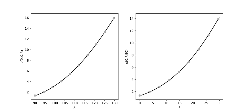
Figure 1 shows the approximate solution $\mathcal{U}_{0}$ obtained by the DNN algorithm; details on the training procedure are given in Remark 4.1.

Figure 1. Solution $u(0,l,\lambda)$ for $l=0$, $\lambda\in[90,130]$ (left) and $l\in[0,30]$, $\lambda=90$ (right) computed with the DNN-algorithm (black line) and reference points computed with Monte-Carlo (grey dots).

As a reference we compute for fixed $(l,\lambda)$ approximate values $U^{MC}(l,\lambda)\approx u(0,l,\lambda)$ with Monte-Carlo using $10^{6}$ simulated paths for each point $(l,\lambda)$ (paths are simulated with the Euler-Maruyama scheme). The relative $L^{1}$-error between the DNN approximation $\mathcal{U}$ and the MC-solution $U^{MC}$ is defined as

$$\epsilon:=\mathbb{E}\Big{[}\Big{|}\frac{\mathcal{U}(\xi^{l},\xi^{\lambda})-{U}^{MC}(\xi^{l},\xi^{\lambda})}{{U}^{MC}(\xi^{l},\xi^{\lambda})}\Big{|}\Big{]}.$$ (4.4)

Using 1000 simulations of $\xi^{l}\sim\text{Unif}([0,30]),\xi^{\lambda}\sim\text{Unif}([90,130])$ we obtained a relative error of $\epsilon=0.0018$. On a Lenovo Thinkpad notebook with an Intel Core i5 processor (1.7 GHz) and 16 GB of memory the computation of $\mathcal{U}$ via the training of a DNN took around 322 seconds, whereas the computation of $U^{MC}(l,\lambda)$ with Monte-Carlo for a fixed point $(l,\lambda)$ took around 4.3 seconds. This shows that the DNN approach is faster than the MC approach if one wants to compute $u(t,l_{i},\lambda_{i})$ for a grid $(l_{i},\lambda_{i})$ with more than 100 grid points. Note also that the training of the networks can be accelerated further by using GPU computing.

Remark 4.1 (Details regarding the numerical implementation).

Our choice of the network architecture largely follows [3]. Throughout we use a DNN with 2 hidden layers. In the reinsurance example we worked with 50 nodes for the hidden layers. For a payoff of the form (4.2) it is advantageous to use softplus as activation function for the hidden layers and the identity for the output layer. The networks are initialized with random numbers using the Xavier initialization. We use mini-batch optimization with mini-batch size $M=5000$, batch normalization and 10000 epochs for training. We minimize the loss function with the Adam optimizer and decrease learning rate from 0.1 to 0.01, 0.001 and 0.0001 after a 2000, 4000 and 6000 epochs.

4.2. Ruin probability of an insurer with different business lines

In the second case study we consider a non-life insurer who provides financial protection against losses from earthquakes, storms and floods over a given time horizon $T=1$. The occurrence of these natural disasters is modeled using independent Poisson counting processes $N^{E},N^{S},N^{F}$ with constant intensities $\lambda^{E},\lambda^{S},\lambda^{F}$. The magnitudes of hazards caused by earthquakes, storms or floods are modeled by iid sequences $\{E_{n}\}_{n\in\mathbb{N}}$, $\{S_{n}\}_{n\in\mathbb{N}}$, $\{F_{n}\}_{n\in\mathbb{N}}$ of positive random variables.

Furthermore we consider catastrophic events that cause simultaneous losses in the windstorm and flood business lines. These events follow a Poisson process $N^{S,F}$ with constant intensity $\lambda^{S,F}$ and iid claim sizes sequences $\{\widetilde{S}_{n}\}_{n\in\mathbb{N}}$, $\{\widetilde{F}_{n}\}_{n\in\mathbb{N}}$. Define $\lambda=(\lambda^{E},\lambda^{S},\lambda^{F},\lambda^{S,F})\in\mathbb{R}^{5}_{+}$. Then the risk process $X=(X_{t}^{E},X_{t}^{S},X_{t}^{F})_{t\geq 0}$ is given by

$$X^{E}_{t} =b^{E}t+\sigma^{E}W_{t}^{E}-\sum_{n=1}^{N^{E}_{t}}E_{n}\,,\quad t\geq 0,\qquad\textit{(earthquake)}$$ (4.5)

$$X^{S}_{t} =b^{S}t+\sigma^{S}W_{t}^{S}-\sum_{n=1}^{N^{S}_{t}}S_{n}-\sum_{n=1}^{N^{S,F}_{t}}\widetilde{S}_{n}\,,\quad t\geq 0,\qquad\textit{(storm)}$$ (4.6)

$$X^{F}_{t} =b^{F}t+\sigma^{F}W_{t}^{F}-\sum_{n=1}^{N^{F}_{t}}F_{n}-\sum_{n=1}^{N^{S,F}_{t}}\widetilde{F}_{n},\quad t\geq 0,\qquad\textit{(flood)}$$ (4.7)

where $W=(W_{t}^{E},W_{t}^{S},W_{t}^{F})_{t\geq 0}$ is a $3$-dimensional standard Brownian motion, $\sigma=(\sigma^{E},\sigma^{S},\sigma^{F})\in\mathbb{R}^{3}_{+}$ and $b=(b^{E},b^{S},b^{F})\in\mathbb{R}^{3}$. The continuous terms $b^{i}t+\sigma^{i}W^{i}_{t},\,i\in\{E,S,F\}$ are an approximation of the difference of cumulative premium payments and small losses up to time $t$ for each business line. We assume that all claim sizes $E,S,F,\widetilde{S},\widetilde{F}$ are Gamma($\alpha_{i}$,$\beta_{i}$) distributed for $i\in I:=\{1,2,3,4,5\}$. The generator of $X$ is given by

$$\mathcal{L}u(t,x)=\sum_{i=1}^{3}u_{x_{i}}(t,x)b^{i}+\frac{1}{2}\sum_{i=1}^{3}u_{x_{i}x_{i}}(t,x)(\sigma^{i})^{2}+\int_{\mathbb{R}_{+}^{3}}[u(t,x-z)-u(t,x)]\nu(\mathrm{d}z),$$

where $\nu(\mathrm{d}z)=\sum_{i=1}^{3}\lambda^{i}f_{\alpha_{i},\beta_{i}}(z_{i})\mathrm{d}z_{i}+\lambda^{4}f_{\alpha_{4},\beta_{4}}(z_{2})f_{\alpha_{5},\beta_{5}}(z_{3})\mathrm{d}z_{2}\mathrm{d}z_{3}.$

We define the ruin time $\tau<T$ as the first time the minimum of all three risk processes falls below zero, i.e. $\tau:=\inf\{t\geq 0\colon\min(X^{E}_{t},X^{S}_{t},X^{F}_{t})\leq 0\}$. Define the set $D:=(0,\infty)^{3}\subset\mathbb{R}^{3}$ and note that $\tau$ is the first exit time of the risk process $X$ from $D$. Put

$$g(t,x)=\begin{cases}0,\quad t=T,x\in D,\\ 1,\quad t\leq T,x\notin D.\end{cases}$$

The ruin probability $u$ at time $t\in[0,T]$ given $\tau>t$ is

$$u(t,x):=\mathbf{P}(\tau\leq T\mid X_{t}=x)=\mathbb{E}[g(T\wedge\tau,X_{T\wedge\tau})|X_{t}=x],\quad x\in D.$$ (4.8)

By standard arguments $u$ is the unique solution of the linear PIDE

$$u_{t}(t,x)+\mathcal{L}u(t,x)=0,\quad(t,x)\in[0,T)\times D,$$ (4.9)

with boundary condition $v(t,x)=g(t,x)$.

We approximate $x\mapsto u(0,x)$ on $A:=[0.1,5]^{3}$ with a deep neural network $\mathcal{U}_{0}$ assuming that $\xi\sim\text{Unif}(A)$. Moreover we compare the result to Monte-Carlo approximations $U^{MC}(x)$ for fixed points $x\in A$. Table 2 contains the parameters we use.

$\sigma$	$b$	$\lambda$	$\alpha$	$\beta$
$(0.1,0.1,0.1)$	$(6,6,6)$	$(2,2,10,1)$	$(3,2,0.5,2,1)$	$(1,1,1,1,1)$

Table 2. Parameters used for the case study on ruin probabilities. Recall that claim sizes are Gamma$(\alpha_{i},\beta_{i})$ distributed.

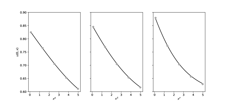
Figure 2 shows the approximate solution $\mathcal{U}_{0}(x)\approx u(0,x)$ obtained by the DNN algorithm on the sections $\{(x^{E},3,3)\colon x^{E}\in[0.1,5]\}$, $\{(3,x^{S},3)\colon x^{S}\in[0.1,5]\}$ and $\{(3,3,x^{F})\colon x^{F}\in[0.1,5]\}$. The network architecture is as in Remark 4.1, but since we are working in $d=3$ dimensions we choose mini-batch size $M=6000$ and 100 nodes for the hidden layers. To verify our result we computed $U^{MC}(x)\approx u(0,x)$ with Monte-Carlo for fixed $x\in A$ using $2\cdot 10^{6}$ path simulations for each point. The relative error (4.4) was computed to $\epsilon=0.0016$ (using 1000 simulations of $\xi\sim\text{Unif}(A)$), which is again very small. Training of the network took around 740 seconds; the computation of the reference solution via Monte Carlo took around 20 seconds per point.

This example clearly shows the advantages of the DNN method over standard Monte Carlo for computing the solution on the entire set $A$. Suppose that we want to compute the solution on $[0.1,5]^{3}$ (as in our case study). Even the very coarse grid $\{1,2,\dots,5\}^{3}$ has already 125 gridpoints, and computing the solution for each gridpoint takes approximately $20\times 125=2500$ seconds, which is about three times the time for training the network.

Figure 2. Solution $u(0,x)$ on $\{(x^{E},3,3)\colon x^{E}\in[0.1,5]\}$ (left), $\{(3,x^{S},3)\colon x^{S}\in[0.1,5]\}$ (middle), and $\{(3,3,x^{F})\colon x^{F}\in[0.1,5]\}$ (right) with the DNN-algorithm (black line) and Monte-Carlo (grey dots).

5. Deep learning approximation for semilinear PIDEs

Next we consider semilinear PIDEs of the form

$$u_{t}(t,x) +\mathcal{L}u(t,x)+f(t,x,u(t,x),\nabla u(t,x))=0,\quad(t,x)\in[0,T)\times D,$$ (5.1)

$$u(t,x) =g(t,x),\quad(t,x)\in\big{(}[0,T)\times(\mathbb{R}^{d}\setminus D)\big{)}\cup\big{(}\{T\}\times\mathbb{R}^{d}\big{)}\,.$$ (5.2)

Here $f\colon[0,T]\times\mathbb{R}^{d}\times\mathbb{R}\times\mathbb{R}^{d}\to\mathbb{R}$ is a nonlinear function and the integro-differential operator $\mathcal{L}$ is given by (2.3). Our goal is to extend the deep splitting approximation method developed by Beck et al. [4] for semilinear PDEs without boundary conditions to the more general equation (5.1). Moreover, we propose an approach for improving the performance of the method. In the derivation of the deep splitting method we implicitly assume that a classical solution of this PIDE exists; see for instance Davis and Lleo [14] for results on this issue.

5.1. Basic method

We divide the interval $[0,T]$ into subintervals using a time grid $0=t_{0}<t_{1}<\dots<t_{N}=T$ and we let $\Delta t_{n}=t_{n}-t_{n-1}$. Suppose that $u^{*}$ is the unique solution of the PIDE (5.1). Define for a fixed $u\in\mathcal{C}^{0,1}([0,T]\times D)$ the function

$$(t,x)\mapsto f_{[u]}(t,x)=f(t,x,u(t,x),\nabla u(t,x)).$$

Then $u^{*}$ also solves the linear PIDE

$$u_{t}(t,x)+\mathcal{L}u(t,x)+f_{[u^{*}]}(t,x)=0.$$ (5.3)

Applying the Feynman-Kac formula to the linear PIDE (5.3) we get the following representation for $u^{*}$

$${u}^{*}(t_{n-1},x)=\mathbb{E}\Big{[}u^{*}(t_{n}\wedge\tau,X^{x}_{t_{n}\wedge\tau})+\int_{t_{n-1}}^{t_{n}\wedge\tau}f_{[u^{*}]}(s,X^{x}_{s})\mathrm{d}s\Big{]},\quad x\in D.$$ (5.4)

Here $X^{x}$ solves the SDE (2.1) with initial condition $X_{t_{n-1}}^{x}=x$, that is

$$X^{x}_{t}=x+\int_{t_{n-1}}^{t}\mu(s,X_{s}^{x})\ \mathrm{d}s+\int_{t_{n-1}}^{t}\sigma(s,X_{s}^{x})\ \mathrm{d}W_{s}+\int_{t_{n-1}}^{t}\int_{\mathbb{R}^{d}}\gamma(s,X_{s-}^{x},z)\ J(\mathrm{d}z,\mathrm{d}s),$$

and the stopping time $\tau$ is given by $\tau=\inf\{s>t_{n-1}\colon X^{x}_{s}\notin D\}$. In the deep splitting method proposed in [4] the integral term in (5.4) is approximated by the endpoint rule

$$\int_{t_{n-1}}^{t_{n}}f_{[u^{*}]}(s,X^{x}_{s})\mathrm{d}s\approx f_{[u^{*}]}(t_{n},X^{x}_{t_{n}})\Delta t_{n}\,.$$ (5.5)

An approximate solution $\mathcal{U}_{n}(\cdot)\approx u^{*}(t_{n},\cdot)$, $n=0,\dots N$ is then found by backward induction over the grid points. The solution at the maturity $t_{N}=T$ is defined using the terminal condition, that is ${\mathcal{U}}_{N}(x):=g(T,x).$ Given $\mathcal{U}_{n}$ we then compute $\mathcal{U}_{n-1}$, $n=1,2,\dots,N$ as follows. First we put

$$\tilde{u}(t_{n-1},x) :=\mathbb{E}\Big{[}{\mathcal{U}}_{n}(X^{x}_{t_{n}}){\mathbf{1}}_{\{\tau>t_{n}\}}+g(\tau,X^{x}_{\tau}){\mathbf{1}}_{\{\tau\leq t_{n}\}}$$ (5.6)

$$+(t_{n}\wedge\tau-t_{n-1})f\big{(}t_{n}\wedge\tau,X^{x}_{t_{n}\wedge\tau},{\mathcal{U}}_{n}(X^{x}_{t_{n}\wedge\tau}),\nabla{\mathcal{U}}_{n}(X^{x}_{t_{n}\wedge\tau})\big{)}\Big{]}\,.$$ (5.7)

We then compute $\mathcal{U}_{n-1}\approx\tilde{u}(t_{n-1},\cdot)$ by applying the regression based DNN algorithm method from Section 3. In this step it is important to work with DNNs with a smooth activation function so that $\nabla{\mathcal{U}}_{n}$ is well-defined.

Remark 5.1.

An additional complication may arise if the domain $D$ is unbounded. In that case we compute the approximate solution on some bounded set $A_{n}\subset D$ and we have to make sure that the set $A_{n}$ is big enough so that the probability of generating paths with $X_{t_{n-1}}\in A_{n-1}$ but $X_{t_{n}}\notin A_{n}$ is sufficiently small so that these paths can be ignored without affecting the training procedure. There are various ways to achieve this, see Beck et al. [4] for details.

5.2. Alternative method

Next we discuss an alternative linearization procedure based on the midpoint rule

$$\int_{t_{n-1}}^{t_{n}}f_{[u^{*}]}(s,X^{x}_{s})\mathrm{d}s\approx f_{[u^{*}]}\left(\overline{t}_{n},X^{x}_{\overline{t}_{n}})\right)\Delta t_{n}\,.$$ (5.8)

Here $\overline{t}_{n}=(t_{n-1}+t_{n})/2$ is the midpoint of the interval $[t_{n-1},t_{n}]$. It is well known that (5.8) usually provides a better approximation to an integral than the endpoint rule (5.5). We therefore propose the following approximation scheme based on the midpoint rule. In a first step we apply the approximation (5.6) over the smaller interval $[\overline{t}_{n},t_{n}]$; this yields an approximate solution $\overline{\mathcal{U}}_{n}$ at $\overline{t}_{n}$. Next we define

$$\tilde{u}(t_{n-1},x) :=\mathbb{E}\bigg{[}{\mathcal{U}}_{n}(X^{x}_{t_{n}}){\mathbf{1}}_{\{\tau>t_{n}\}}+g(\tau,X^{x}_{\tau}){\mathbf{1}}_{\{\tau\leq t_{n}\}}$$ (5.9)

$$+(t_{n}\wedge\tau-t_{n-1})f\big{(}\overline{t}_{n}\wedge\tau,X^{x}_{\overline{t}_{n}\wedge\tau},\overline{\mathcal{U}}_{n}(X^{x}_{\overline{t}_{n}\wedge\tau}),\nabla\overline{\mathcal{U}}_{n}(X^{x}_{\overline{t}_{n}\wedge\tau})\big{)}\bigg{]}\,;$$ (5.10)

as before, a numerical approximation $\mathcal{U}_{n-1}$ to $\tilde{u}(t_{n-1},x)$ is computed via the deep learning algorithm from Section 3. Our numerical experiments in Section 6 show that the approximation based on the midpoint rule performs significantly better than the original deep splitting method from Beck et al. [4].

Remark 5.2 (Convergence results).

Germain et al. [17] recently obtained a convergence result for the deep splitting method for PDEs. They consider only Cauchy problems (no boundary conditions) and they make strong Lipschitz assumptions on the coefficients of the equation. Under these conditions they come up with an estimate for the approximation error in terms of the mesh of the partition $t_{0},\dots,t_{N}$ and the size of the DNN used in the individual time steps. We are confident that similar results can be obtained for PIDEs. However, theoretical convergence results are of limited practical use for designing an effective DNN approximation to PIDEs, and we leave this technical issue for future work.

6. Examples for the semilinear case

In this section we test the algorithm in two case studies. First we consider the well-known stochastic regulator problem. This problem leads to a semilinear PIDE with an explicit solution that can be used as a validity check for our methods. The second case study is an actuarial example dealing with the optimization of an insurance portfolio under transaction costs and risk capital constraints.

6.1. Stochastic regulator problem

The first example is the stochastic linear regulator. Denote by $c=(c_{1,t},\dots,c_{d,t})_{t\geq 0}$ an adapted control strategy and consider the controlled $d$-dimensional process $\widetilde{X}^{c}$ with dynamics

$$d\widetilde{X}_{i,t}=c_{i,t}\ \mathrm{d}t+\sigma_{i}\mathrm{d}W_{i,t}+\int_{\mathbb{R}}z\ \widetilde{J_{i}}(\mathrm{d}z,\mathrm{d}t),\;1\leq i\leq d,\qquad\widetilde{X}_{0}=x\in\mathbb{R}^{d}\,.$$ (6.1)

Here $W=(W_{1},\dots,W_{d})$ is a $d$-dimensional standard Brownian motion, $\theta\in\mathbb{R}^{d}$, $\rho\in\mathbb{R}^{d}$, $\sigma_{1},\dots,\sigma_{d}$ are positive constants, $T>0$ and $\widetilde{J}_{1},\dots,\widetilde{J}_{d}$ is the compensated jump measure of $d$ independent compound Poisson processes with Gamma($\alpha_{i},\beta_{i}$)-distributed jumps. Denote by $\mathcal{A}$ the set of all adapted $d$-dimensional processes $c$ with $\mathbb{E}\Big{[}\int_{0}^{T}|c_{s}|^{2}\mathrm{d}s\Big{]}<\infty$ and consider the control problem

$$u(t,x)=\inf_{c\in\mathcal{A}}\mathbb{E}\bigg{[}\sum_{i=1}^{d}\Big{(}\int_{t}^{T}\big{(}(\widetilde{X}_{i,s}^{c})^{2}+\theta_{i}c_{i,s}^{2}\big{)}\,\mathrm{d}s+\rho_{i}(\widetilde{X}_{i,T}^{c})^{2}\Big{)}\,\Big{|}\,\widetilde{X}_{t}^{c}=x\bigg{]},\quad t\in[0,T],\,x\in\mathbb{R}^{d}.$$

The interpretation of this problem is that the controller wants to drive the process $\widetilde{X}$ to zero using the control $c$; the instantaneous control cost (for instance the energy consumed) is measured by $\theta c^{2}_{t}$. At maturity $T$ the controller incurs the terminal cost $\rho\widetilde{X}_{T}^{2}$.

The Hamilton-Jacobi-Bellman (HJB) equation associated to this control problem is

$$u_{t}(t,x) +\frac{1}{2}\sum_{i=1}^{d}\sigma_{i}^{2}u_{x_{i}x_{i}}(t,x)+\int_{\mathbb{R}^{d}}\Big{[}u(t,x+z)-u(t,x)-\sum_{i=1}^{d}z_{i}u_{x_{i}}(t,x)\Big{]}\nu(\mathrm{d}z)$$

$$+\sum_{i=1}^{d}x_{i}^{2}+\inf_{c}\Big{\{}\sum_{i=1}^{d}c_{i}u_{x_{i}}(t,x)+\theta_{i}c_{i}^{2}\Big{\}}=0,\quad(t,x)\in[0,T)\times\mathbb{R}^{d},$$

with terminal condition $u(T,x)=\varphi(x):=\sum_{i=1}^{d}\rho_{i}x_{i}^{2}$. The minimum in the HJB equation is attained at $c_{i}^{*}(t,x)=-\frac{1}{2\theta_{i}}\frac{\partial u}{\partial x_{i}}(t,x)$, so that the value function solves the semilinear PIDE

$$u_{t}(t,x) +\frac{1}{2}\sum_{i=1}^{d}\sigma_{i}^{2}u_{x_{i}x_{i}}(t,x)-\sum_{i=1}^{d}\int_{\mathbb{R}^{d}}z_{i}\ \nu(\mathrm{d}z)u_{x_{i}}(t,x)$$ (6.2)

$$+\int_{\mathbb{R}^{d}}[u(t,x+z)-u(t,x)]\ \nu(\mathrm{d}z)+\sum_{i=1}^{d}x_{i}^{2}-\sum_{i=1}^{d}\frac{1}{4\theta_{i}}u_{x_{i}}(t,x)^{2}=0\,.$$ (6.3)

It is well known that the HJB equation (6.2) can be solved analytically, see also [30]. For this we make the Ansatz $u(t,x)=\sum_{i=1}^{d}a^{i}(t)x_{i}^{2}+b(t).$ Substitution into (6.2) gives an ODE system for $a(t)$ and $b(t)$ that can be solved explicitly. One obtains

$$a^{i}(t) =\sqrt{\theta_{i}}\frac{1+\kappa_{i}e^{2t/\sqrt{\theta}}}{1-\kappa_{i}e^{2t/\sqrt{\theta}}},\qquad\kappa_{i}:=\frac{\rho_{i}-\sqrt{\theta_{i}}}{\rho_{i}+\sqrt{\theta_{i}}}e^{-\frac{2T}{\sqrt{\theta_{i}}}}$$

$$b(t) =\sum_{i=1}^{d}\sqrt{\theta_{i}}\Big{(}\sigma_{i}^{2}+\int_{\mathbb{R}^{d}}z_{i}^{2}\ \nu(\mathrm{d}z)\Big{)}\Big{(}(T-t)+\log\big{(}(1-\kappa_{i}e^{2t})/(1-\kappa_{i}e^{2T})\big{)}\Big{)}.$$

To test the deep splitting method we computed $u(t,x)$ for $x\in A:=[-2,2]^{d}$ numerically. For this we partition the time horizon into $N=10$ intervals $0=t_{0}<t_{1}<\dots<t_{N}=T$ and simulate the auxiliary process $X$ for $t\in[t_{n-1},t_{n}]$

$$X_{i,t}=\xi_{i}+\int_{t_{n-1}}^{t}\sigma_{i}\ \mathrm{d}W_{i,s}+\int_{t_{n-1}}^{t}\int_{\mathbb{R}}z\ J_{i}(\mathrm{d}z,\mathrm{d}s)-\int_{t_{n-1}}^{t}\Big{(}\int_{\mathbb{R}}z\ \nu_{i}(\mathrm{d}z)\Big{)}\ \mathrm{d}s,\quad 1\leq i\leq d,$$ (6.4)

where $W$ and $J$ are as in (6.1), and where $\xi$ is uniformly distributed on $A$. The nonlinear term is finally given by

$$f(t,x,y,z)=\sum_{i=1}^{d}\Big{(}x_{i}^{2}-\frac{1}{4\theta_{i}}z_{i}^{2}\Big{)}.$$

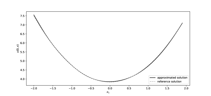
We use the midpoint rule (5.8) to linearize the PIDE and approximate $x\mapsto u(t_{n},x)$ with a deep neural network $\mathcal{U}_{n}$ for $n=0,1,\dots,N-1$; details on numerics are given in Remark 6.1. Figure 3 shows the approximate solution of $u$ obtained by the deep splitting method and the analytic reference solution. Table 3 contains the parameters used.

As in the linear case the relative $L^{1}$-error for a deep neural network approximation $\mathcal{U}_{n}$ at time $t=t_{n}$ is defined as

$$\epsilon_{t_{n}}:=\mathbb{E}\bigg{[}\Big{|}\frac{\mathcal{U}_{n}(\xi)-u(t_{n},\xi)}{u(t_{n},\xi)}\Big{|}\bigg{]}.$$ (6.5)

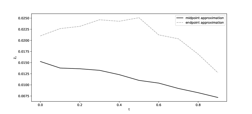
Using 10000 simulations of $\xi$ we approximate the relative error $\epsilon_{t}$ (6.5) for $t=t_{0},t_{1},\dots,t_{N-1}$. In particular, for $i=1,\dots,10$ and $n=0,1,\dots,{N-1}$ we train different networks $\mathcal{U}^{i}_{n}$ with error $\epsilon^{i}_{t_{n}}$ to compute the average error, i.e. $\bar{\epsilon_{t}}=\frac{1}{10}\sum_{i=1}^{10}\epsilon^{i}_{t}$ for $t=t_{n},\ n=0,1,\dots,{N-1}$. The training for the whole network, that consists of 20 sub-networks (10 DNNs at $t_{n}$ and 10 DNNs at midpoints $\bar{t}_{n}$), took around 7500 seconds. Figure 4 compares the error $\bar{\epsilon}$ of the midpoint method to the averaged relative $L^{1}$-error computed with the endpoint rule (5.5) with $N=10$. Clearly, the method based on the midpoint rule performs substantially better than the standard method based on the endpoint rule. Note that even though we use $N=10$ for both methods the midpoint rule requires training of 20 networks. However our experiments showed that the midpoint rule with $N=10$ discretization steps also outperforms the endpoint rule with $N=20$ steps.

$T$	$d$	$\sigma$	$\theta$	$\rho$	$\lambda$	$\alpha$	$\beta$
1	4	$(0.1,\dots,0.1)$	$(1,\dots,1)$	$(0.5,\dots,0.5)$	$(10,\dots,10)$	$(0.4,\dots,0.4)$	$(4,\dots,4)$

Table 3. Parameters used in the stochastic regulator problem

Figure 3. Explicit solution $u(0,x)$ (grey) and DNN-approximation $\mathcal{U}(x)$ (black) on $\{x=(x_{1},1,1,1):x_{1}\in[-2,2]\}$.

Figure 4. Comparison of the averaged relative $L^{1}$-error $\bar{\epsilon}_{t}$ of the endpoint (grey) and the midpoint (black) approximation for $N=10$.

Remark 6.1 (Details on the numeric implementation).

We used a similar network architecture as in [4]. We worked with deep neural networks with 2 hidden layers consisting of 100 nodes each. All neural networks are initialized with random numbers using the Xavier initialization. We use mini-batch optimization with mini-batch size $M=5000$, batch normalization and 12000 training epochs. The loss function is minimized with the Adam optimizer and decreasing learning rate from 0.1 to 0.01, 0.001, 0.0001 and 0.00001 after 2000, 4000, 6000 and 8000 epochs. We use sigmoid as activation function for the hidden layers and the identity for the output layer. All computations were run on a Lenovo Thinkpad notebook with an Intel Core i5 processor (1.7 GHz) and 16 GB memory.

6.2. Optimal insurance portfolios with risk capital constraints

The second case study is an optimization problem in insurance. We consider a stylized model of an insurance company who dynamically optimizes her holdings of some insurance portfolio in the presence of transaction costs and risk capital constraints. Without of capital constraints the problem admits an analytic solution and is therefore a useful test case. With capital constraints the model leads to a semilinear boundary value problem for which there is no explicit solution, and we study this case numerically using the deep splitting method. In fact, the analysis of the impact of risk capital constraints on optimal insurance portfolios is also interesting in its own right.

Consider an insurer who invests into an insurance portfolio with market value $S_{t}$ at time $t$ and in cash. We assume that the process $S$ has dynamics

$$\mathrm{d}S_{t}=\bar{\mu}\mathrm{d}t+\sigma\mathrm{d}W_{t}-\mathrm{d}R_{t},$$

Here the Brownian motion $W$ models the compensated small claims, the compound Poisson process $R$ with intensity $\lambda$ and jump size distribution $\eta(\mathrm{d}z)$ models the large claims, and $\bar{\mu}>0$ is the premium income of the portfolio. We assume that the insurance portfolio can be adjusted only gradually over time. In mathematical terms this means that the insurer uses an absolutely continuous trading strategy with trading rate $\theta=(\theta_{t})_{0\leq t\leq T}$, so that for a given strategy $\theta$, the size $Q^{\theta}$ of the insurance portfolio satisfies $\mathrm{d}Q_{t}^{\theta}=\theta_{t}\ \mathrm{d}t$. We assume that Moreover, the insurer incurs a transaction cost that is proportional to the trading rate $\theta_{t}^{2}$. This models the fact that a rapid adjustment of the insurance portfolio is expensive, as the insurer needs to carry out costly marketing activities or to enter into expensive reinsurance contracts. Given a parameter $\kappa>0$ modelling the size of the transaction cost, the cash position $C^{\theta}$ has dynamics

$$\mathrm{d}C_{t}^{\theta}=-\big{(}\theta_{t}S_{t}+\kappa\theta_{t}^{2}\big{)}\mathrm{d}t\,.$$

Here the term $-\theta_{t}S_{t}\mathrm{d}t$ gives the revenue from trading the insurance position and the term $-\kappa\theta_{t}^{2}\mathrm{d}t$ models the reduction of the cash position due to transaction costs. From a mathematical viewpoint this model is fairly similar to models used in the literature on optimal portfolio execution such as Cardaliaguet and LeHalle [7] or Cartea et al. [8].

Denote by $E_{t}^{\theta}=S_{t}Q_{t}^{\theta}+C_{t}^{\theta}$ the insurer’s equity. We assume that the insurer wants to maximize the expected value of her equity position $E_{T}^{\theta}$ at some horizon date time $T$, and that she incurs a liquidation cost of size $\gamma({Q_{T}^{\theta}})^{2}$ for some parameter $\gamma>0$. Note that for a given strategy $\theta$ the process $(Q^{\theta},E^{\theta})$ has dynamics

$$\mathrm{d}Q_{t}^{\theta} =\theta_{t}\ \mathrm{d}t,$$ (6.6)

$$\mathrm{d}E_{t}^{\theta} =Q_{t}^{\theta}\bar{\mu}\mathrm{d}t+Q_{t}^{\theta}\sigma\mathrm{d}W_{t}-Q_{t}^{\theta}\mathrm{d}R_{t}-\kappa\theta_{t}^{2}\ \mathrm{d}t.$$

Hence the pair $(Q^{\theta},E^{\theta})$ is Markov and we may use this process as state process. We define the value function of the insurers optimization problem for $t\in[0,T]$ as

$$u(t,q,e):=\sup_{\theta\in\mathcal{A}}\mathbb{E}\big{[}E_{T}^{\theta}-\gamma(Q_{T}^{\theta})^{2}\mid Q_{t}^{\theta}=q,\ E_{t}^{\theta}=e\big{]}\,,$$ (6.7)

where $\mathcal{A}$ denotes the set of all adapted trading rates such that $E\big{[}\int_{0}^{T}\theta_{t}^{2}\mathrm{d}t\big{]}<\infty$.

To prevent early ruin regulatory institutions usually impose risk capital constraints. In particular they may liquidate an insurance company if the equity is too low compared to the size of the company’s insurance portfolio. Below we use the deep splitting method to study how capital constraints affects the value function and the optimal strategy of the reinsurer. Before that we consider the unconstraint problem. In that case there exists an explicit solution to the HJB equation (PIDE (6.11) below), which can be used to test the performance of the deep splitting method.

6.2.1. The case without constraints

By standard arguments the HJB equation associated with the problem (6.7) is

$$u_{t}(t,q,e) +q\bar{\mu}u_{e}(t,q,e)+\frac{1}{2}\sigma^{2}q^{2}u_{ee}(t,q,e)+\lambda\int_{0}^{\infty}\![u(t,q,e+qz)-u(t,q,e)]\eta(\mathrm{d}z)$$ (6.8)

$$+\sup_{\theta\in\mathbb{R}}\{\theta u_{q}(t,q,e)-\kappa\theta^{2}u_{e}(t,q,e)\}=0,$$ (6.9)

with terminal condition $u(T,q,e)=e^{2}-\gamma q^{2}$. Maximization gives the candidate optimal trading rate

$$\theta_{t}^{*}(t,q,e)=\frac{1}{2\kappa}\frac{u_{q}(t,q,e)}{u_{e}(t,q,e)};$$ (6.10)

substitution into (6.8) yields the semilinear PIDE

$$u_{t}(t,q,e) +q\bar{\mu}u_{e}(t,q,e)+\frac{1}{2}\sigma^{2}q^{2}u_{ee}(t,q,e)+\lambda\int_{0}^{\infty}[u(t,q,e+qz)-u(t,q,e)]\ \eta(\mathrm{d}z)$$ (6.11)

$$+\frac{1}{4\kappa}\frac{u_{q}(t,q,e)^{2}}{u_{e}(t,q,e)}=0\,.$$ (6.12)

To solve the case without constraints we make the Ansatz $u(t,q,e)=e+v(t,q)$, that is we assume that $u$ is linear in the equity value $e$. This implies

$$\lambda\int_{0}^{\infty}[u(t,q,e+qz)-u(t,q,e)]\eta(\mathrm{d}z)=\lambda q\int_{0}^{\infty}z\eta(\mathrm{d}z)=:q\lambda\bar{\eta}.$$

If we define $\bar{\alpha}=\bar{\mu}-\lambda\bar{\eta}$, (6.11) reduces to the following the following first order PDE for $v$

$$-\bar{\alpha}q=v_{t}(t,q)+\frac{v_{q}(t,q)^{2}}{4\kappa}\,,$$ (6.13)

with terminal condition $v(T,q)=-\gamma q^{2}$. To find an explicit solution for $v$ we follow Cardaliaguet and LeHalle [7] and make the Ansatz $v(t,q)=h_{0}(t)+h_{1}(t)q-\frac{1}{2}h_{2}(t)q^{2}.$ Substitution in the HJB equation (6.13) gives the following ODE system for $h_{0},h_{1},h_{2}$

$$h_{2}^{\prime}=h_{2}^{2}/(2\kappa),\qquad h_{1}^{\prime}=-\bar{\alpha}+h_{1}h_{2}/(2\kappa),\qquad h_{0}^{\prime}=-h_{1}^{2}/(4\kappa)$$

with terminal condition $h_{0}(T)=h_{1}(T)=0$ and $h_{2}(T)=2\gamma$. The ODEs can be solved explicitly: one has

$$h_{2}(t) =\frac{2\kappa}{T+\frac{\kappa}{\gamma}-t},$$

$$h_{1}(t) =\frac{c_{1}+\frac{1}{2}\bar{\alpha}t^{2}-a\bar{\alpha}t}{a-t},\text{ where }c_{1}:=-\frac{1}{2}\bar{\alpha}T^{2}+a\bar{\alpha}T\text{ and }a:=T+\frac{\kappa}{\gamma},$$

$$h_{0}(t) =\frac{1}{4\kappa(a-t)}\Big{(}-\frac{2}{3}\bar{\alpha}^{2}a^{4}+\frac{2}{3}\bar{\alpha}^{2}a^{3}t+2\bar{\alpha}a^{2}c_{1}+\bar{\alpha}c_{1}t^{2}-2\bar{\alpha}ac_{1}t-c_{1}^{2}+\frac{1}{12}\bar{\alpha}^{2}t^{4}-\frac{1}{3}\bar{\alpha}^{2}at^{3}\Big{)}.$$

For comparison purposes we computed the solution $u(t,x)=u(t,q,e)$ of (6.11) with the deep splitting algorithm on the set A:=$\{(q,e)\colon-7\leq q\leq 7,0\leq e\leq 6\}$. For this we partition the time horizon into $N=10$ intervals $0=t_{0}<t_{1}<\dots<t_{N}=T$ and simulate the auxiliary process $X=(X^{Q},X^{E})$ with $X^{Q}_{t}=\xi^{Q}$ and

$$X^{E}_{t} =\xi^{E}+\int_{t_{n-1}}^{t}X^{Q}_{s}\bar{\mu}\ \mathrm{d}s+\int_{t_{n-1}}^{t}X^{Q}_{s}\sigma\ \mathrm{d}W_{s}+\int_{t_{n-1}}^{t}\int_{\mathbb{R}}X^{Q}_{s}z\ J(\mathrm{d}z,\mathrm{d}s)\,,$$ (6.14)

where $\xi=(\xi^{Q},\xi^{E})$ is uniformly distributed on $[-7,7]\times[0,7]$, $W$ is a Brownian motion and $J$ is a jump measure with compensating measure $\nu=\lambda\eta$ for $\eta$ a Gamma distribution with parameters $\alpha$ and $\beta$. Moreover, we identify the nonlinear term in the PIDE to

$$f(t,x,y,z)=\frac{1}{4\kappa}\frac{z_{1}^{2}}{z_{2}}.$$

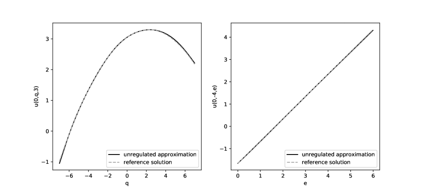
We used the midpoint rule (5.8) to linearize the PIDE. The network architecture was as in Remark 6.1. The training for the whole network that consists of 20 subnetworks (a DNN for every grid point $t_{n}$, $0\leq n\leq 9$ and a DNN for every midpoint $\bar{t}_{n}$) took around 4400 seconds. Table 4 contains the parameters used in the experiment. Figure 5 shows the approximate solution $\mathcal{U}_{0}$ obtained by the deep splitting algorithm and the analytic reference solution.

$\sigma$	$\gamma$	$\kappa$	$\bar{\mu}$	$\lambda$	$\alpha$	$\beta$
$0.1$	$0.1$	$0.1$	$0.8$	$5$	$0.4$	$4$

Table 4. Parameters for the optimal insurance problem

Figure 5. Solution of the unconstraint insurance problem for $q\in[-7,7]$, $e=3$ (left) and $q=-4$, $e\in[0,6]$ (right) with the DNN-algorithm (black) and reference solution (grey).

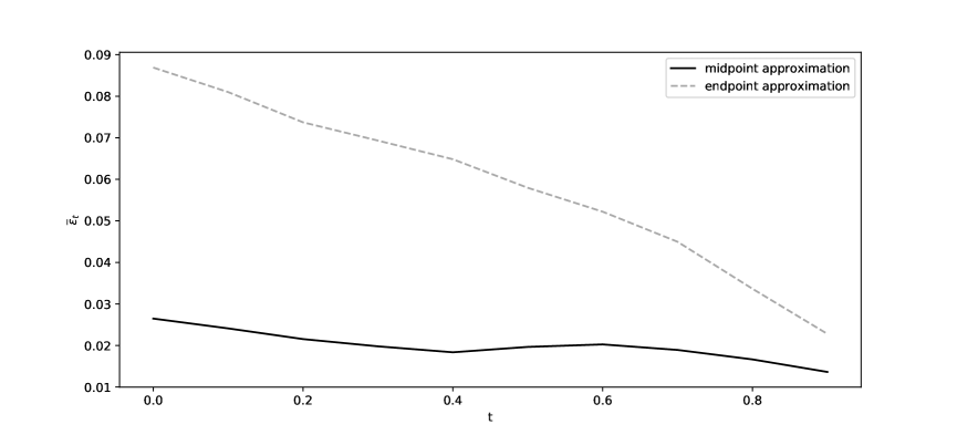
As the solution $u$ can be zero we report the absolute $L^{1}$-error between the DNN approximation $\mathcal{U}_{n}$ and the analytic solution, that is $\varepsilon_{t_{n}}^{\text{abs}}:=\mathbb{E}\Big{[}\big{|}{\mathcal{U}_{n}(\xi)-u(t_{n},\xi)}\big{|}\Big{]}.$ To compute the absolute error we used 10000 simulations of $\xi=(\xi^{Q},\xi^{E})$ where $\xi^{Q}\sim\text{Unif}([-7,7])$ and $\xi^{E}\sim\text{Unif}([0,6])$ Figure 6 illustrates the mean error of 10 different DNN approximations $\mathcal{U}^{i}_{n},\,i=1,\dots,10$, i.e. using once the midpoint rule and once the original method from [4]. We see that the algorithm based on the midpoint rule performs substantially better than the original deep splitting method.

Figure 6. Comparison of the two different training methods illustrating the averaged absolute $L^{1}$-error $\bar{\varepsilon}_{t}^{\text{abs}}$ using endpoint (grey) and midpoint (black) approximation in 10 training procedures.

6.2.2. The optimization problem with constraints.

Next we discuss the optimization problem under risk capital constraints. We expect that risk capital constraints will alter the investment decisions of the insurer since she wants to avoid a liquidation of the company. To set up the corresponding optimization problem we need to specify the set $D$ of acceptable positions of the insurer and the liquidation value of the company given that its position exits from $D$. For numerical reasons it is convenient to model $D$ as a bounded set. Given large constants $\bar{e}$ and $\bar{q}$ and a parameter $\delta>0$ we define the set $D$ of acceptable positions as

$$D=\{(q,e)\in\mathbb{R}^{2}\colon|q|<\bar{q},\ \delta|q|<e<\bar{e}\}\,.$$ (6.15)

The constraint $e>\delta|q|$ implies that before liquidation the solvency ratio $|Q_{t}|/E_{t}$ of the insurer is bounded by $\delta^{-1}$, so that $\delta^{-1}$ can be viewed as a measure of the regulator’s risk tolerance. We assume that the liquidation value of the insurance company on the boundary of $D$ is given by the value $u^{\text{unreg}}$ of the company in the unconstraint problem, reduced by a penalty $k(t,q,e)\geq 0$, and we set

$$g(t,q,e)=u^{\text{unreg}}(t,q,e)-k(t,q,e).$$

Here $k:[0,T]\times[-\bar{q},\bar{q}]\times[0,\bar{e}]\rightarrow[0,\infty)$ is a smooth function that penalizes exit from the set of acceptable positions. We assume that $k(t,q,\bar{e})=0,0\leq t\leq T$ (no penalization for high equity values) and that $k(T,q,e)=0,\ 0\leq e\leq\bar{e}$ (no penalization at maturity). In our numerical experiments we take $\bar{e}=10^{6}$ $\delta=1$, and $k(t,q,e)=0.5(T-t)(\bar{e}-e)/\bar{e}$; the other parameters are identical to the unconstraint case, see Table 4.

The value function for the problem with risk capital constraints is

$$u^{\text{reg}}(t,q,e)=\sup_{\theta\in\mathcal{A}}\mathbb{E}\big{[}g(\tau\wedge T,Q^{\theta}_{\tau\wedge T},E^{\theta}_{\tau\wedge T})|Q_{t}=q,\ E_{t}=e\big{]},\quad t\in[0,T],\,(q,e)\in D\,,$$

where $\tau=\inf\{s\geq t\colon(Q^{\theta},E^{\theta})\notin D\}$. The PIDE associated with this control problem and the form of the optimal strategy are the same as in the unregulated case (see (6.8) and (6.10)), but now we have in addition the boundary condition

$$u(t,q,e)=u^{\text{unreg}}(t,q,e)-k(t,q,e),\quad t\in[0,T),\,(q,e)\notin D\,.$$

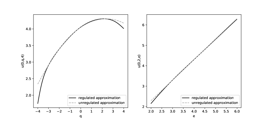
Due to the boundary condition the Ansatz $u^{\text{reg}}(t,q,e)=e+v(t,q)$ does not hold and we had to compute $u^{\text{reg}}$ via the deep splitting algorithm. In view of its superior performance in the unconstraint case we worked with the midpoint procedure, and we used the same network architecture as in the unconstraint case. We worked on the set $A=\{(q,e)\colon-e\leq q\leq e,0\leq e\leq 6\}\subset D$. Figure 7 illustrates the DNN-approximation for $u^{\text{reg}}(0,q,e)$ and $u^{\text{unreg}}(0,q,e)$ on the sections $\{(q,4):q\in[-4,4]\}$ and $\{(2,e):e\in[2,6]\}$. The right plot shows that with risk capital constraints the value function is concave in $e$ and for $e\approx 2$ significantly lower than $u^{\text{unreg}}$ (for $\delta=1$ the point $(q,e)=(2,2)$ belongs to the lower bound of $D$).

Figure 7. DNN-approximations of $u^{reg}(0,q,e)$ (black) and $u^{unreg}(0,q,e)$ (grey) on the section $\{(q,4):q\in[-4,4]\}$ (left) and on $\{(2,e):e\in[2,6]\}$ (right).

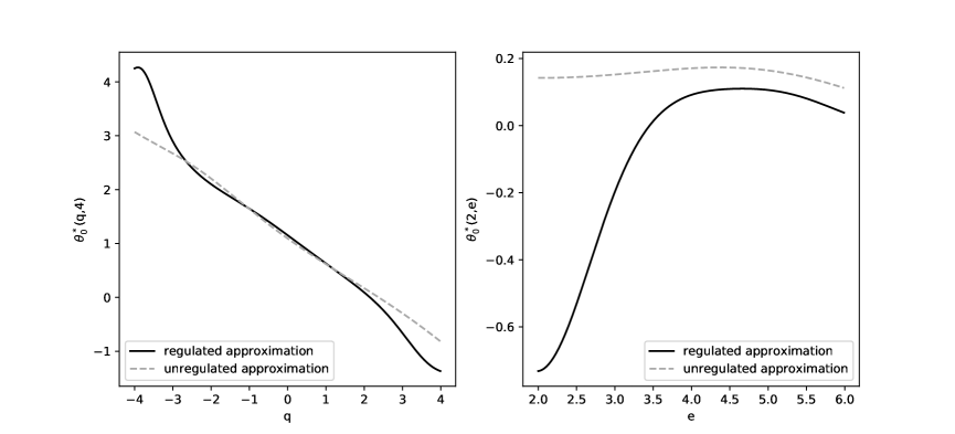
The optimal trading rate is plotted in Figure 8. The plots show that the optimal strategy differs from the optimal strategy in the unregulated case as the insurer wants to reduce the size $|\theta_{t}^{*}|$ of his risky position in order to avoid liquidation. For instance, in the right plot the optimal trading rate for $q=2$ is negative for $e$ close to 2. This is quite intuitive: the insurer wants to reduce her insurance portfolio as the equity value approaches the boundary of $D$ in order to avoid a costly liquidation.

Figure 8. DNN-approximations of the optimal strategy $\theta_{0}^{*}$ for the regulated case (black) and the unregulated case (grey) on $\{(q,4):q\in[-4,4]\}$ (left) and on $\{(2,e):e\in[2,6]\}$ (right).

7. Conclusion

In this paper we studied two deep neural network algorithms for solving linear and semilinear parabolic PIDEs from insurance mathematics. To assess the performance of our methodology we carried out extensive tests for several multi-dimensional PIDEs arising in typical actuarial pricing and control problems. In all test cases the performance of the proposed approximation algorithms was quite satisfying in terms of accuracy and speed. This suggests that deep neural network algorithms might become a useful enhancement of the toolbox for solving many valuation and control problems in insurance that can be phrased in terms of a PIDE.

References

• Al-Aradi et al. [2019] A. Al-Aradi, A. Correia, D. d. F. Naiff, G. Jardim, and Y. Saporito. Applications of the Deep Galerkin Method to solving partial integro-differential and Hamilton-Jacobi-Bellman equations. arXiv preprint arXiv:1912.01455, 2019.
• Andersen and Andreasen [2000] L. Andersen and J. Andreasen. Jump-diffusion processes: Volatility smile fitting and numerical methods for option pricing. Review of Derivatives Research, 4(3):231–262, 2000.
• Beck et al. [2018] C. Beck, S. Becker, P. Grohs, N. Jaafari, and A. Jentzen. Solving stochastic differential equations and Kolmogorov equations by means of deep learning. arXiv preprint arXiv:1806.00421, 2018.
• Beck et al. [2019] C. Beck, S. Becker, P. Cheridito, A. Jentzen, and A. Neufeld. Deep splitting method for parabolic PDEs. arXiv preprint arXiv:1907.03452, 2019.
• Bensoussan and Lions [1982] A. Bensoussan and J.-L. Lions. Impulse Control and Quasi-Variational Inequalities. Dunod, Paris, 1982.
• Briani et al. [2007] M. Briani, R. Natalini, and G. Russo. Implicit–explicit numerical schemes for jump–diffusion processes. Calcolo, 44(1):33–57, 2007.
• Cardaliaguet and LeHalle [2018] P. Cardaliaguet and C. A. LeHalle. Mean field game of controls and an application to trade crowding. Mathematics and Financial Economics, 12:335–363, 2018.
• Cartea et al. [2015] Á. Cartea, S. Jaimungal, and J. Penalva. Algorithmic and high-frequency trading. Cambridge University Press, 2015.
• Casella and Roberts [2011] B. Casella and G. O. Roberts. Exact simulation of jump-diffusion processes with monte carlo applications. Methodology and Computing in Applied Probability, 13(3):449–473, 2011.
• Castro [2021] J. Castro. Deep learning schemes for parabolic nonlocal integro-differential equations. arXiv preprint arXiv:2103.15008, 2021.
• Ceci et al. [2020] C. Ceci, K. Colaneri, R. Frey, and V. Köck. Value adjustments and dynamic hedging of reinsurance counterparty risk. SIAM Journal on Financial Mathematics, 11(3):788–814, 2020.
• Colaneri and Frey [2021] K. Colaneri and R. Frey. Classical solutions of the backward PIDE for Markov modulated marked point processes and applications to CAT bonds. Insurance: Mathematics and Economics, forthcoming, 2021.
• Cont and Voltchkova [2005] R. Cont and E. Voltchkova. A finite difference scheme for option pricing in jump diffusion and exponential lévy models. SIAM Journal on Numerical Analysis, 43(4):1596–1626, 2005.
• Davis and Lleo [2013] M. Davis and S. Lleo. Jump-diffusion risk-sensitive asset management ii: jump-diffusion factor model. SIAM Journal on Control and Optimization, 51(2):1441–1480, 2013.
• E et al. [2017] W. E, J. Han, and A. Jentzen. Deep learning-based numerical methods for high-dimensional parabolic partial differential equations and backward stochastic differential equations. Communications in Mathematical Statistics, 5:349–380, 2017.
• Ethier and Kurtz [1986] S. Ethier and T. G. Kurtz. Markov Processes: Characterization and Convergence. Wiley, New York, 1986.
• Germain et al. [2020] M. Germain, H. Pham, and X. Warin. Deep backward multistep schemes for nonlinear PDEs and approximation error analysis. arXiv preprint arXiv:2006.01496, 2020.
• Gihman and Skohorod [1980] I. Gihman and A. Skohorod. The Theory of Stochastic Processes, volume III. Springer, New York, 1980.
• Giles [2008] M. B. Giles. Multilevel Monte Carlo path simulation. Operations research, 56(3):607–617, 2008.
• Glasserman [2003] P. Glasserman. Monte Carlo Methods in Financial Engineering. Springer, New York, 2003.
• Grandell [2012] J. Grandell. Aspects of Risk Theory. Springer Science & Business Media, 2012.
• Han and Long [2020] J. Han and J. Long. Convergence of the deep bsde method for coupled fbsdes. Probability, Uncertainty and Quantitative Risk, 5(1):1–33, 2020.
• Han et al. [2018] J. Han, A. Jentzen, and E. Weinan. Solving high-dimensional partial differential equations using deep learning. Proc. Nat. Acad. Sci. USA, 115:8505–8510, 2018.
• Huré et al. [2020] C. Huré, H. Pham, and X. Warin. Deep backward schemes for high-dimensional nonlinear PDEs. Mathematics of Computation, 89(324):1547–1579, 2020.
• Kliemann et al. [1990] W. Kliemann, G. Koch, and F. Marchetti. On the unnormalized solution of the filtering problem with counting process observations. IEEE, IT-36:1415–1425, 1990.
• Kremsner et al. [2020] S. Kremsner, A. Steinicke, and M. Szölgyenyi. A deep neural network algorithm for semilinear elliptic PDEs with applications in insurance mathematics. Risks, 8(4):136, 2020.
• Kwon and Lee [2011] Y. Kwon and Y. Lee. A second-order finite difference method for option pricing under jump-diffusion models. SIAM journal on numerical analysis, 49(6):2598–2617, 2011.
• Matache et al. [2004] A.-M. Matache, T. Von Petersdorff, and C. Schwab. Fast deterministic pricing of options on Lévy driven assets. ESAIM: Mathematical Modelling and Numerical Analysis, 38(1):37–71, 2004.
• Metwally and Atiya [2002] S. A. Metwally and A. F. Atiya. Using brownian bridge for fast simulation of jump-diffusion processes and barrier options. The journal of derivatives, 10(1):43–54, 2002.
• Øksendal and Sulem [2007] B. K. Øksendal and A. Sulem. Applied stochastic control of jump diffusions, volume 498. Springer, 2007.
• Pham [1998] H. Pham. Optimal stopping of controlled jump diffusion processes: a viscosity solution approach. Journal of Mathematical Systems, Estimation and Control, 8:1–27, 1998.
• Pham et al. [2021] H. Pham, X. Warin, and M. Germain. Neural networks-based backward scheme for fully nonlinear PDEs. SN Partial Differential Equations and Applications, 2(1):1–24, 2021.
• Sirignano and Spiliopoulos [2018] J. Sirignano and K. Spiliopoulos. DGM: A deep learning algorithm for solving partial differential equations. Journal of Computational Physics, 375:1339–1364, 2018.