The Hilti SLAM Challenge Dataset

Abstract

Research in Simultaneous Localization and Mapping (SLAM) has made outstanding progress over the past years. SLAM systems are nowadays transitioning from academic to real world applications. However, this transition has posed new demanding challenges in terms of accuracy and robustness. To develop new SLAM systems that can address these challenges, new datasets containing cutting-edge hardware and realistic scenarios are required. We propose the Hilti SLAM Challenge Dataset. Our dataset contains indoor sequences of offices, labs, and construction environments and outdoor sequences of construction sites and parking areas. All these sequences are characterized by featureless areas and varying illumination conditions that are typical in real-world scenarios and pose great challenges to SLAM algorithms that have been developed in confined lab environments. Accurate sparse ground truth, at millimeter level, is provided for each sequence. The sensor platform used to record the data includes a number of visual, lidar, and inertial sensors, which are spatially and temporally calibrated. The purpose of this dataset is to foster the research in sensor fusion to develop SLAM algorithms that can be deployed in tasks where high accuracy and robustness are required, e.g., in construction environments. Many academic and industrial groups tested their SLAM systems on the proposed dataset in the Hilti SLAM Challenge. The results of the challenge, which are summarized in this paper, show that the proposed dataset is an important asset in the development of new SLAM algorithms that are ready to be deployed in the real-world.

Supplementary Material

The dataset as well as information regarding the Hilti SLAM Challenge is available at https://www.hilti-challenge.com. The results of the Hilti SLAM Challenge were also presented in a talk: https://www.youtube.com/watch?v=3oqTGrnSkrY&t=685s

I Introduction

Recent years have seen outstanding progresses in SLAM [1]. The transition from demonstrative to real-world applications is happening at this moment. A promising application of SLAM for autonomous robotics is in construction sites. Construction robotics offers a way to remove hazards for workers, improve task productivity, and collect high-quality data [2]. However, these environments bring many challenges to SLAM systems. Featureless scenes, varying illumination conditions, and sudden motions are among the main challenges.

The deployment of SLAM algorithms to real-world applications has shed light on the limitations of the current systems. These limitations are being addressed by academic research often in collaboration with industrial partners [3]. We believe that collaborations between academia and industry have the potential to accelerate the process of developing new SLAM systems that are able to meet tight requirements in terms of accuracy and robustness.

An important role in this phase is played by the availability of datasets containing relevant scenarios and sensors. The scenarios should portray actual real-world applications where SLAM systems are deployed. As the robotic community has shown in several works [4, 5, 6], the highest accuracy and robustness is achieved by fusing multiple and complementary sensors. For this reason, SLAM datasets should contain multiple sensor modalities.

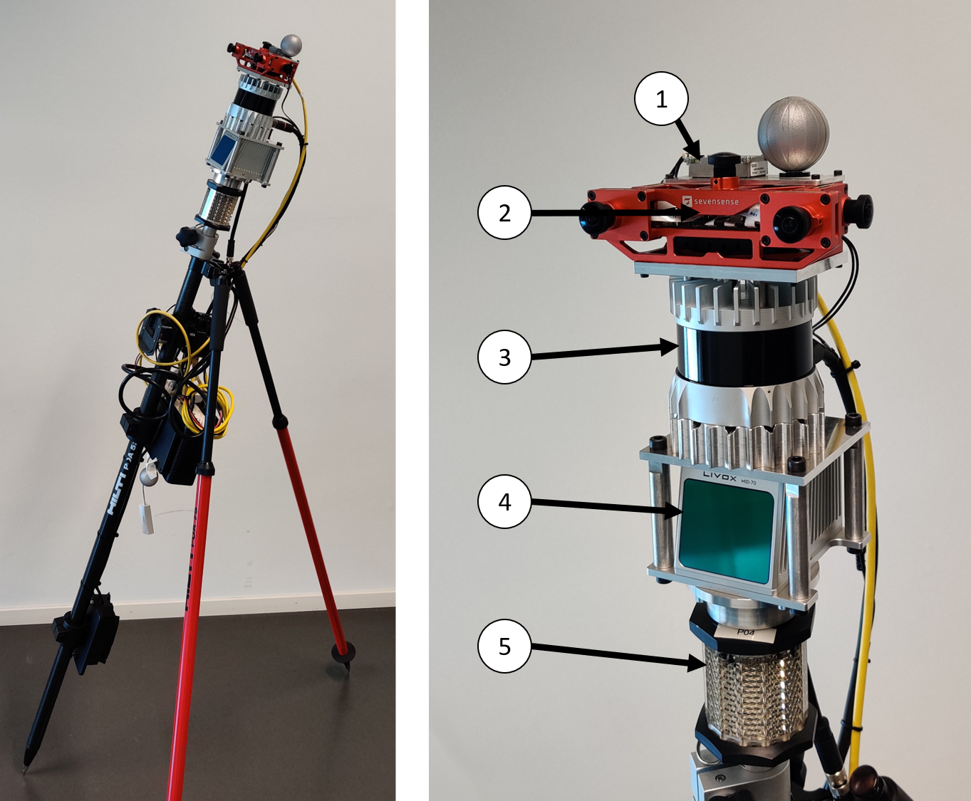
Figure 1: Left: The full sensor stick resting on a tripod. Right: (1) ADIS16445 IMU (2) AlphaSense 5-camera module (3) Ouster OS0-64 LiDAR (4) Livox MID70 LiDAR (5) prism for the Total Station.

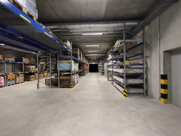
(a) Basement

(b) Campus

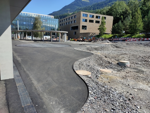
(c) Construction Site

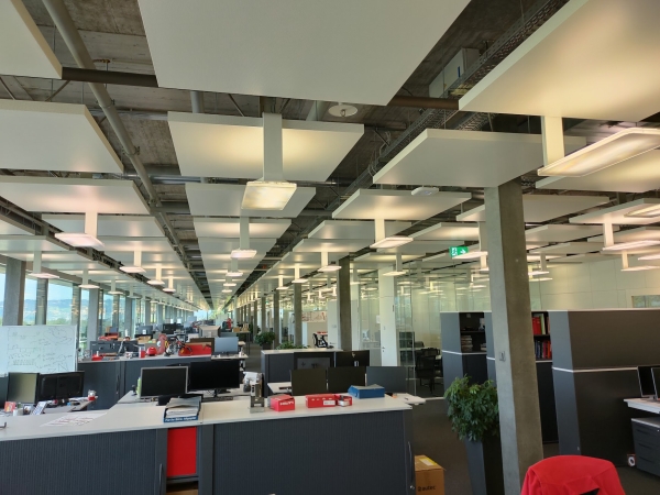
(d) IC Office

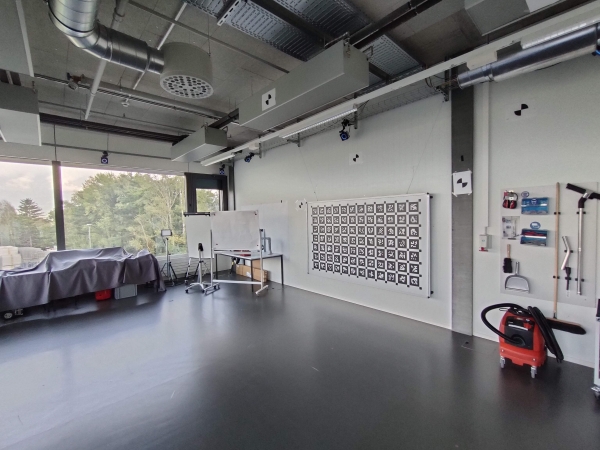
(e) Lab

(f) Office Mitte

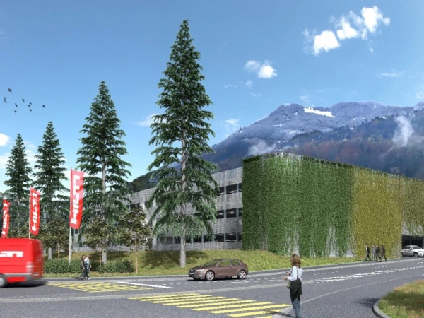
(g) Parking

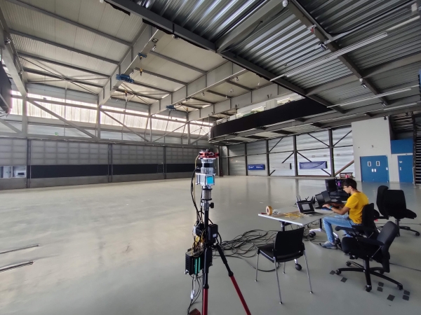
(h) RPG Tracking Area

Figure 2: Locations where the dataset have been captured.

Many SLAM datasets have been proposed over the past years [7, 8, 9, 10, 11, 12, 13, 14, 15, 16, 17, 18], each of them has specific contributions on the availability of multiple sensors and the type of scenarios and motions. Most of the datasets [7, 9, 12, 13, 14, 15, 16, 17] focus on visual and inertial data, while only a few [8, 10, 11] also provide LiDAR data. Depending on the type of environment and motion, each dataset poses different challenges to SLAM. Visual and inertial data recorded onboard an unmanned aerial vehicle (UAV) in [7, 17] bring difficulties to visual-inertial odometry (VIO) and SLAM systems because of fast motions. Varying illumination conditions and moving objects are the main challenges of datasets recorded in autonomous driving scenarios [9, 8, 19]. Sudden motions and low texture, as well as dynamic illumination conditions, are the main challenges of datasets recorded with a handheld sensor platform [10, 11, 12, 14, 15].

We propose the Hilti SLAM Challenge Dataset. The purpose of this dataset is to foster the research in sensor fusion to develop SLAM algorithms that can be deployed in tasks where high accuracy, at millimeter level, and robustness are required, e.g., in construction environments. Our dataset contains indoor sequences of construction sites, offices, and labs and outdoor sequences of construction environments and parking areas (in Fig.  2). All these sequences are characterized by featureless areas and varying illumination conditions that are typical of real-world scenarios and pose challenges to SLAM algorithms that have been developed in confined lab environments. Millimeter accurate ground truth by mean of a motion capture system (MoCap) or a Total Station [20], is provided for each sequence. To record the data, we have created a suite of sensors including a number of visual, LiDAR, and inertial sensors, using the latest products in commercially available sensing technologies with particular attention made to time synchronization and spatial calibration. With the use of redundant sensors, this dataset also directly compares sensor performance in different environments, which can be informative for the design of SLAM systems. With this dataset, we aim to stimulate research on robust indoor positioning, mapping, and navigation with the particular application to construction environments.

This dataset was used in the Hilti SLAM Challenge, where many academic and industrial groups submitted their SLAM systems. The results of the challenge, which are summarized in Section V, show that the proposed dataset can be an important asset in the development of new SLAM algorithms that are ready to be deployed in the real-world.

To summarize, the main contributions of the Hilti SLAM Challenge Dataset are:

• Real-world sequences recorded in indoor offices and labs, indoor and outdoor construction environments, and outdoor parking areas containing challenging featureless areas and varying illumination conditions.

• Sensor suite containing 5 cameras (1 stereo pair), 2 lidars, and 3 IMUs with accurate spatial and temporal calibration.

• The Hilti SLAM Challenge. Many academic and industrial groups used this dataset to further develop their SLAM systems and take part in the Hilti SLAM Challenge competition.

II Related Work

TABLE I: Comparison of SLAM datasets

Dataset	Num. seq,	Environment	Motion	Sensors	Synchronization	Ground truth
EuRoC [7]	11	Indoor	UAV	1 Stereo camera 1 IMU	Hw	Laser tracker, MoCap
KITTI [8]	22	Outdoor	Car	1 Stereo camera 1 Stereo RGB camera 1 Lidar 1 IMU	Sw	GNSS-INS
Malaga [9]	15	Outdoor	Car	1 Stereo RGB camera 1 IMU	Sw	GPS
The Newer College Dataset [11]	3	In- / Outdoor	Handheld	4 Cameras 1 Lidars 2 Imus	Hw / Sw	3D imaging laser scanner, ICP
PennCOSYVIO [12]	4	In- / Outdoor	Handheld	4 RGB cameras 1 Stereo camera 1 Fisheye camera 2 IMUs	Hw / Sw	Fiducial markers
TartanAir [13]	30	In- / Outdoor	Simulation	Synthetic 1 stereo RGB camera	Sim.	Simulation
TUM VIO [14]	28	In- / Outdoor	Handheld	1 Stereo camera 1 IMU	Hw	MoCap (start, end)
UMA VI [15]	32	In- / Outdoor	Handheld	1 Stereo RGB camera 1 Stereo camera 1 IMU	Hw	Pose alignment (start, end)
UMich [16]	27	In- / Outdoor	UGV	6 RGB cameras 1 IMU	Sw	Fusion of GPS, IMU, laser
UZH-FPV [17]	28	In- / Outdoor	UAV	1 Stereo camera 1 Event camera 2 IMUs	Hw / Sw	Fusion of vision, IMU, laser
The Hilti SLAM Challenge Dataset (Ours)	12	In- / Outdoor	Handheld	5 Cameras 2 Lidars 3 Imus	Hw / Sw	MoCap, Total Station

Among the plethora of datasets proposed to benchmark SLAM, as well as VIO, systems, [7, 8, 9, 10, 11, 12, 13, 14, 15, 16, 17, 18] are the ones that mostly relate to the Hilti SLAM Challenge Dataset. Many datasets [7, 9, 12, 13, 14, 15, 16, 17] focus on visual and inertial data. The datasets [7, 17] provide hardware-synchronized visual, from a stereo camera, and inertial data recorded on board an UAV. They challenge SLAM algorithms because of fast motions, with [17] containing the most aggressive maneuvers. For both datasets, the ground truth is generated by solving a bundle adjustment problem including visual, inertial, and laser tracker data. In [7], some sequences provide ground truth data for a MoCap system. The datasets [12, 14, 15] provide visual and inertial data recorded using a handheld sensor platform. In all these datasets, the sensor platform includes a stereo camera and an IMU. In addition, stereo RGB cameras are also available in [12, 15]. The ground truth in [12] is obtained by localizing to fiducial markers, which are placed along the trajectory. The ground truth at the start and end of the trajectory is obtained by pose alignment with respect to fiducial markers and using a MoCap system in [15] and [14], respectively. In [13], it was proposed a large (30 sequences) simulated dataset containing a broad range of scenarios. The dataset in [18] includes data from an event camera, a survey on event vision is presented in  [21], as well as a standard camera and IMU. It was designed to incentivize researchers to investigate the use of event cameras in SLAM. The datasets [9, 8, 16] contain data recorded in autonomous driving, and ground robot navigation, scenarios. They all include RGB cameras and an IMU. The dataset [8] is one of the most used datasets for benchmarking SLAM systems in autonomous driving. It also includes LiDAR data. The ground truth for these datasets is provided by inertial navigation systems (INS) aided by global navigation satellite systems (GNSS). The dataset proposed in [11], which is an extension of [10], is the closest to our dataset. It contains sequences recorded in a university campus. The sensor platform includes 4 cameras, 1 LiDAR, and 2 IMUs. The ground truth is provided by an iterative closest point [22] (ICP) algorithm that registers the LiDAR point cloud to a prior map. Differently from [11], our dataset provides millimeter accurate ground truth from the Hilti PLT 300  automated Total Station or a MoCap system. In fact, the focus of our dataset is to advance the state-of-the-art in SLAM in terms of accuracy with the final target of developing systems that are able to achieve millimeter level accuracy as required in construction environments.

III Hardware

Our sensor suite (the ’Phasma’ stick, Fig. 1) consists of 3 categories of sensing modalities operating with different ranges and noise levels. These include:

III-A Passive Visual

• Alphasense by Sevensense
  The visual data is collected from an array of rigidly mounted 1.3 MP global shutter cameras. This module consists of 5 wide field-of-view cameras mounted to give an approximate 270 deg continuous field of view. Within this configuration, a stereo pair is present. Images are synchronously collected at 10 Hz. While the Alphasense can capture at a higher frame rate, doing so would have required using a lower resolution. Since this dataset aims for maximum accuracy, the higher resolution was chosen.

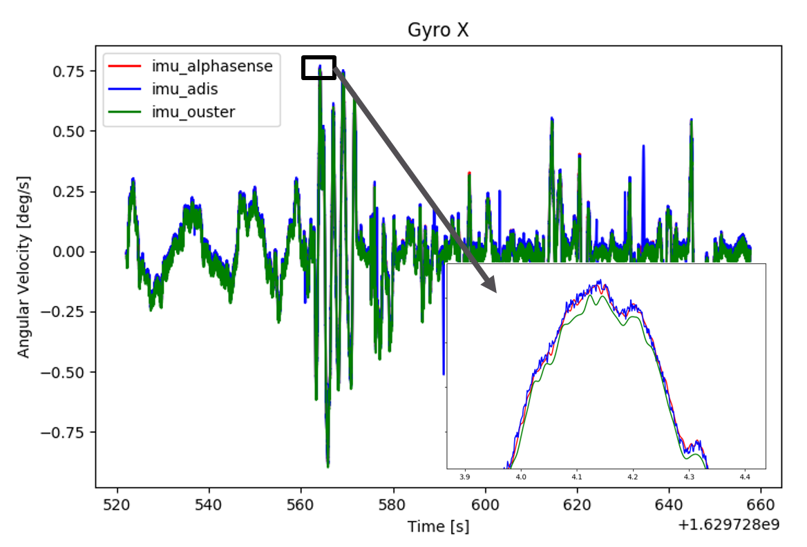
Figure 3: Verification of the time synchronization between the LiDAR and the camera module. The gyroscope data show a difference of <1ms.

III-B Active Optical

• Ouster OS0-64
  Long-range point cloud data is collected by the 360 deg scanning LiDAR sensor. This unit has a scan repetition of 10 Hz, and a point data rate of 1,300,000 points/second. Ranges are recorded from 0.3 to 50 m, with typical lowest noise returns greater than 1 m. Range accuracy is 1.5-5 cm.
  

• Livox MID70
  This unit is a LiDAR sensor with a 70 deg circular field of view and a non-repeating scan pattern. Point data rate is 100,000 points/second. Ranges are recorded from 0.02 to 200 m, with typical returns between 1 and 50 m. Range accuracy is 2-5 cm.

III-C Inertial Sensors

• Analog Devices ADIS16445
  This IMU is rigidly mounted to the AlphaSense module. It is a high-performing MEMS based sensor with relatively low noise and sensor bias drift rates. The data from this IMU is tightly timestamped to the AlphaSense timing system. Data is collected at 800 Hz.
  

• Bosch BMI085
  This IMU is embedded in the AlphaSense module. It provides a modest level of performance in terms of noise and bias stability. The data from this IMU is tightly timestamped to the AlphaSense timing system. Data is collected at 200 Hz.
  

• InvenSense ICM-20948
  This IMU is embedded in the Ouster LiDAR. It provides a more modest level of performance than the ADIS16445 in terms of noise and bias stability. The data from this IMU is tightly timestamped to the Ouster timing system. Data is collected at 100 Hz.

III-D Ground Truth System

For testing and validation, 2 systems are used to capture the ground truth:

• Total Station
  A survey grade prism is attached to the Phasma stick, tracked by the Hilti PLT 300 automated Total Station. Ground truth data is collected in a ”stop ’n  go” fashion, where the total station precisely measures the prism during the ’stop’ periods. The stick is gravity aligned, using a mechanical system, before collecting each ground truth measurement. The total station range and angle measurements are processed to generate XYZ position information. In this situation, the range measurements of the static prism have accuracy of 3 mm.

• Optical Tracking
  Optical tracking targets are attached to the Phasma stick. When operated in a motion capture space, the multiple targets allow for the direct computation of the 6-DOF pose. Those ground truth data-points have a position accuracy of <1mm and are collected at 200 Hz.

III-E DATA SYNCHRONIZATION AND LOGGING

In a dynamic multi-sensor system, time synchronization between sensors is critical to make the best use of sensors fusion. Special care was given to synchronization of the Phasma stick to ensure maximum performance:

• AlphaSense, Bosch IMU and ADIS IMU
  The AlphaSense manages time synchronization at the hardware level via an FPGA implementation. Camera times are computed to the mid-exposure pulse (MEP). Imu data is time tagged on arrival to the FPGA data bus. Overall time synchronization between the cameras and IMUs is <1 ms.
  

• Ouster LiDAR and Invensense IMU
  The Ouster module includes an integrated IMU. The Ouster point data and IMU are hardware synchronized to the Ouster internal clock. Time synchronization between the two sensors is <1ms.
  

• Cross Module Synchronization
  Synchronization between modules (AlphaSense, Ouster, Livox) is provided by the supported PTP network time protocol [23]. Each module is attached via wired Ethernet cable to the data logging device, which hosts the PTP master clock. With this setup, the time alignment between the modules is observed to be <1 ms, as shown in Fig.  3. For verification, we adopted the approach from [24] and used optimization tools over the correlation signal of gyroscope data.
  

Data logging occurs on a dedicated computer connected to the Phasma stick. The logging computer, with the Ubuntu 18.04 OS, runs the Robotic Operating System (ROS) during the data capture. Sensing modules are connected to the data logger, and data streams are directly recorded in ROS bag files.

III-F CALIBRATION

Accurate intrinsic and extrinsic sensors calibration is critical to achieving the highest system performance. Each respective manufacturer conducted intrinsic sensor calibration. We re-run the intrinsic calibration of the cameras using a standard checkerboard calibration. For LiDARs, proprietary calibration models were used and corrections applied to the data at the time of capture.
The reference point of the body frame of the Phasma stick is defined at the AlphaSense Bosch IMU center. All other sensors are transformed back to this point. Extrinsic calibrations were determined from the CAD model of the Phasma design. The calibration procedure proposed in [25] was used to refine the cameras-IMUs extrinsic calibrations. Calibration files, CAD Models, and sensor noise parameters are provided on the dataset website.

IV Dataset

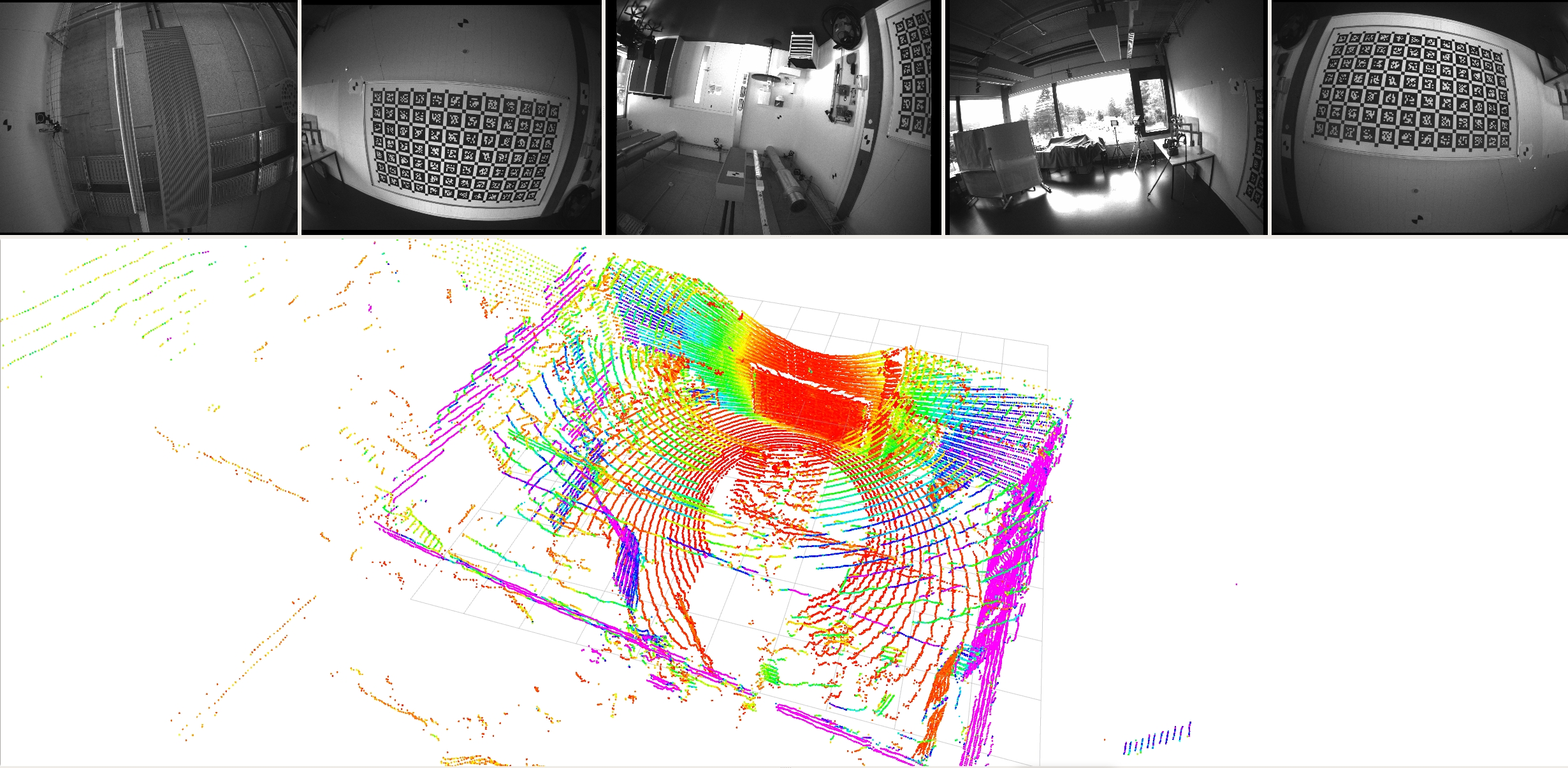
Figure 4: Example from the dataset ’Lab Survey 2’: images from the 5 cameras and the Ouster OS0 point cloud

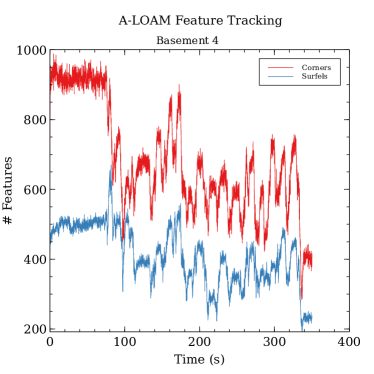
(a)

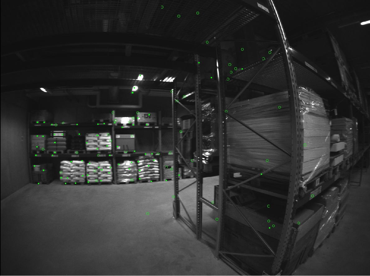
(b)

Figure 5: (a) Features tracked in ’Basement 4’ using the LiDAR-based SLAM algorithm A-LOAM. (b) the local environment during a low LiDAR feature event (time approx. 336 s). Close walls and structures reduce the LiDAR measurements, whereas vision based algorithms can still operate normally (the feature tracks of SVO2 [26] are shown).

Data was collected under various conditions in indoor, outdoor, and mixed indoor-outdoor environments. The data shows practical challenges in different stages of constructions. Challenges include variable lighting, limited features and/or highly reflective and transparent surfaces.

Data descriptions (see Fig. 2):

• Basement
  Data was collected in a windowless room (approx. 20x40 m). No natural light, mixed illumination brightness. Concrete space with building infrastructure. Basement 1 is a short and easy path. In Basement 3 and Basement 4, we mounted the sensor platform on a moving base instead of operating it handheld. Basement 3 and 4 also allow to exploit loop closure capabilities of the SLAM systems.

• Campus
  Data was collected outdoors in a courtyard setting (approx. 40x60 m). Good natural lighting with high illumination. Mixed features with building structure and natural flora.

• Construction Site
  Mostly outdoors with some covered areas (approx. 40x80 m). Strong natural light with high illumination. Unfinished natural surfaces with limited features above the ground plane.

• IC Office
  Indoor space with many windows and reflective surfaces (approx. 10x70 m). Mix of natural and artificial light. Strong illumination at the windows, modest illumination indoors.

• Lab
  Indoor space dominated by large windows (approx. 10x10 m). Strong natural light and reflective surfaces. Optitrack 6-DOF ground truth.

• Office Mitte
  Indoor space in finished office building (approx. 30x50 m). Mix of natural and artificial light. Lots of building structure.

• Parking
  Mix of indoor and outdoor space (approx. 100x100 m). Parking garage from the top floor to the bottom floor. Lighting varies from extreme bright to modest darkness. Ground plane structure on top floor and plenty of building structure on the lower floor.

• RPG Tracking Area
  Indoor test facility (approx. 30x30 m). Mostly artificial light with some natural. Single large room with random motion path throughout. MoCap 6-DOF ground truth.

IV-A Dataset Format

Datasets are stored in binary format (rosbags) which contain images and IMU and LiDAR data. For the data from the Livox a custom message was chosen as it contains additional timing information compared to the standard ROS PointCloud2 message. Fig. 4 shows an example of the camera and LiDAR data from the Lab Survey 2 dataset. Ground truth data is given in a separate file for each dataset, with the filename indicating the reference source (e.g. Construction_Site_prism.txt means the ground truth is in the prism frame). All topics in the bag are listed in Table II.

TABLE II: Message topics and types of the rosbags

Topic	Type	Description
/alphasense/cam0/image_raw	sensor_msgs/Image	front facing camera 1 (right)
/alphasense/cam1/image_raw	sensor_msgs/Image	front facing camera 2 (left)
/alphasense/cam2/image_raw	sensor_msgs/Image	upward facing camera
/alphasense/cam3/image_raw	sensor_msgs/Image	right facing camera
/alphasense/cam4/image_raw	sensor_msgs/Image	left facing camera
/alphasense/imu	sensor_msgs/Imu	Bosch IMU, 200Hz
/alphasense/imu_adis	sensor_msgs/Imu	ADIS16445, 800Hz
/livox/lidar	livox_ros_driver/CustomMsg	Livox MID70
/os_cloud_node/imu	sensor_msgs/Imu	Ivensense, 100Hz
/os_cloud_node/points	sensor_msgs/PointCloud2	Ouster OS0-64
tf_static	tf2_msgs/TFMessage	all transforms between frames

IV-B Challenges

This section includes an example of the challenges contained in our dataset and highlights the need of multiple sensors fusion. In the sequence Basement 4, the number feature tracks by the LiDAR odometry algorithm, A-LOAM [27], remains high (around 1000 per frame) while the Phasma device is in the centre of the room, but it decreases significantly when the device approaches a wall or a close overhang, see in Fig. 5 left. In this case, the accuracy of the estimated trajectory by A-LOAM is negatively affected. However, the decrease of the LiDAR feature tracks can be compensated by the increase of the visual features, see Fig. 5 right. In this case, the best performance can be achieved by an algorithm that fuses camera and LiDAR measurements.

V The Hilti SLAM Challenge

TABLE III: Results of the Hilti SLAM Challenge. The reports including the description of each submission can be found on the dataset website.

Team	Method	Description	Sensors	RMSE [m]	Score
Megvii3D	based on [28]	IEFK based	LiDAR + imu	0,0774	461
Bosch Research	closed-source	graph optimization, Manhattan world	LiDAR + imu	0,0957	457
Vision & Robotics GmbH	based on [29]	tightly coupled MHE, loop closure, BA	LiDAR + imu	0,1010	406
GeoSLAM	closed-source	sliding window, loop closure, BA	LiDAR + imu	0,2602	389
Oxford Robotics Institute	VILENS [30]	tightly coupled, based on factor graphs	camera + LiDAR + imu	0,1546	378
Nanyang Technological University	VIRAL [31]	sliding window, BA	camera + LiDAR + imu	0,2024	346
CMU Doom	closed-source	sliding window + loop closure	camera + LiDAR + imu	0,3592	333
ETH Zürich	Maplab [32]	tightly coupled, graph based	camera + LiDAR + imu	0,7467	288
NPM3D Team, MINES ParisTech	CT-ICP [33]	scan-to-map, no loop closure, no ba	LiDAR	3,6302	273
UC San Diego	closed-source	scan-to-map, imu for undistortion	LiDAR + imu	0,0838	258
C.F Rubio et.al	based on [34]	optimization based	LiDAR + imu	8,6470	228
IVISO	closed-source	graph based approach, no loop closing	camera + imu	0,6135	219
Spectacular AI	HybVIO [35]	MSCKF [36] based, no global ba	camera + imu	0,6758	216

The proposed dataset was used in the Hilti SLAM challenge, which first edition took place at the 2021 IEEE/RSJ IROS conference. Academic and industrial groups submitted the solutions of their SLAM algorithms on all the sequences of the dataset. Participants had access to the ground truth of half of the sequences. The other half was used for evaluation (similarly to what is done in KITTI [8]). An accuracy-dependent score was computed for ranking teams: after SO3 alignment [37] of the estimated trajectory with the ground truth, every single point scored between 10 and 0 points: 10 points for errors below 1 cm, 6 points between 1 cm and 10 cm and 3 points for errors up to 1 m. This format was chosen, instead of computing the ranking based on the RMSE, because in this way we could also consider non-complete or missing trajectories, which would have distorted the ranking otherwise. The choice of the thresholds was based our use-case, which requires sub-cm accuracy. In total, 27 teams participated in the challenge, with 7 commercial companies among them, see Table III. The first four places have been taken by commercial algorithms, which all focused on LiDAR-IMU odometry, showing the maturity and robustness of these approaches. The best team, Megvii, used a variant of FAST-LIO2 [28] and achieved an average error of 9.3 cm on all sequences. Megvii was one of the few teams that merged the Ouster and the Livox LiDAR data, which, together with using all LiDAR points for state estimation, gave them a significant advantage. The best algorithm that fuses vision with LiDAR and imu ranked 5th, VILENS [30] by the Oxford Robotics Institute. The best vision-only solution ranked 12th, with the majority of errors larger than 50 cm. The results show that, unsurprisingly, commercial algorithms outperform academic algorithms. The exact gap, however, was not clear prior to this challenge. The results also show that there is still room for improvement since the winning team did not fuse camera data. Table III shows an overview of the teams and their approaches (teams who decided to stay anonymously are not shown in the table).

VI Known Issues

Despite careful design and execution of the data collection experiments, we are aware of some issues which pose additional challenges for SLAM algorithms and limit the achievable. These include:

• Clock drift and offset: The clock from MoCap and the data logging computer are not hardware-synchronized. We used Ethernet connection and a time-of-arrival time stamping to keep the offset to a minimum, however we observed a difference of around 1-3ms in the two clocks.

• Some frames in the LiDAR, camera and IMU data were dropped due to high load on the controller.

VII Conclusion

In this paper, we described a new public dataset captured with a redundant multi-sensor platform containing visual, inertial, and LiDAR data. The dataset includes a series of real-world scenarios collected with state-of-the-art sensing technologies and high-quality time-synchronization. Our goal is to foster research in SLAM to advance the current state-of-the-art and make SLAM systems ready to be deployed in real-world applications with demanding requirements in terms of accuracy and robustness, such as in construction robotics. The dataset was used in the Hilti SLAM Challenge. The results of the challenge show a picture of the capabilities of the current SLAM algorithms, from both academia and industry, and potential improvements, such as multi-sensors fusion.

VIII Acknowledgments

We thank Danwei Wang from Nanyang Technological University, Singapore, and Yufeng Yue from Beijing Institute of Technology, China, for hosting the challenge in their IROS 2021 workshop.

References

- [1] Cesar Cadena et al. “Past, Present, and Future of Simultaneous Localization and Mapping: Toward the Robust-Perception Age” In IEEE Trans. Robot. 32.6, 2016, pp. 1309–1332
- [2] Hilti AG “Hilti Jaibot”, 2020 URL: https://www.hilti.ca/content/hilti/W1/CA/en/business/business/trends/jaibot.html
- [3] SLAMcore “SLAMcore Spatial Intelligence for Robots and Machines” URL: https://www.slamcore.com/
- [4] S. Leutenegger et al. “Keyframe-Based Visual-Inertial SLAM using Nonlinear Optimization” In Int. J. Robot. Research, 2015
- [5] Giovanni Cioffi, Titus Cieslewski and Davide Scaramuzza “Continuous-Time vs. Discrete-Time Vision-based SLAM: A Comparative Study” In IEEE Robot. Autom. Lett. IEEE, 2022
- [6] César Debeunne and Damien Vivet “A review of visual-LiDAR fusion based simultaneous localization and mapping” In Sensors 20.7 Multidisciplinary Digital Publishing Institute, 2020, pp. 2068
- [7] Michael Burri et al. “The EuRoC micro aerial vehicle datasets” In The International Journal of Robotics Research, 2016
- [8] Andreas Geiger, Philip Lenz and Raquel Urtasun “Are we ready for Autonomous Driving? The KITTI Vision Benchmark Suite” In Conference on Computer Vision and Pattern Recognition (CVPR), 2012
- [9] José-Luis Blanco-Claraco, Francisco-Angel Moreno-Duenas and Javier González-Jiménez “The Málaga urban dataset: High-rate stereo and LiDAR in a realistic urban scenario” In Int. J. Robot. Research 33.2 SAGE Publications Sage UK: London, England, 2014, pp. 207–214
- [10] Milad Ramezani et al. “The newer college dataset: Handheld lidar, inertial and vision with ground truth” In 2020 IEEE/RSJ International Conference on Intelligent Robots and Systems (IROS), 2020, pp. 4353–4360 IEEE
- [11] Lintong Zhang, Marco Camurri and Maurice Fallon “Multi-camera LiDAR inertial extension to the newer college dataset” In arXiv preprint arXiv:2112.08854, 2021
- [12] Bernd Pfrommer, Nitin Sanket, Kostas Daniilidis and Jonas Cleveland “Penncosyvio: A challenging visual inertial odometry benchmark” In 2017 IEEE International Conference on Robotics and Automation (ICRA), 2017, pp. 3847–3854 IEEE
- [13] Wenshan Wang et al. “TartanAir: A Dataset to Push the Limits of Visual SLAM” In 2020 IEEE/RSJ International Conference on Intelligent Robots and Systems (IROS), 2020
- [14] David Schubert et al. “The TUM VI benchmark for evaluating visual-inertial odometry” In 2018 IEEE/RSJ International Conference on Intelligent Robots and Systems (IROS), 2018, pp. 1680–1687 IEEE
- [15] David Zuñiga-Noël, Alberto Jaenal, Ruben Gomez-Ojeda and Javier Gonzalez-Jimenez “The UMA-VI dataset: Visual–inertial odometry in low-textured and dynamic illumination environments” In The International Journal of Robotics Research 39.9 SAGE Publications Sage UK: London, England, 2020, pp. 1052–1060
- [16] Nicholas Carlevaris-Bianco, Arash K Ushani and Ryan M Eustice “University of Michigan North Campus long-term vision and lidar dataset” In The International Journal of Robotics Research 35.9 Sage Publications Sage UK: London, England, 2016, pp. 1023–1035
- [17] Jeffrey Delmerico et al. “Are We Ready for Autonomous Drone Racing? The UZH-FPV Drone Racing Dataset” In IEEE Int. Conf. Robot. Autom. (ICRA), 2019
- [18] Elias Mueggler et al. “The event-camera dataset and simulator: Event-based data for pose estimation, visual odometry, and SLAM” In The International Journal of Robotics Research 36.2 SAGE Publications, 2017, pp. 142–149
- [19] Joel Janai, Fatma Güney, Aseem Behl and Andreas Geiger “Computer vision for autonomous vehicles: Problems, datasets and state of the art” In Foundations and Trends® in Computer Graphics and Vision 12.1–3 Now Publishers, Inc., 2020, pp. 1–308
- [20] Christoph Klug, Clemens Arth, Dieter Schmalstieg and Thomas Gloor “Measurement Uncertainty Analysis of a Robotic Total Station Simulation” In IECON 2018 - 44th Annual Conference of the IEEE Industrial Electronics Society, 2018, pp. 2576–2582
- [21] Guillermo Gallego et al. “Event-based vision: A survey” In IEEE transactions on pattern analysis and machine intelligence 44.1 IEEE, 2020, pp. 154–180
- [22] Paul J Besl and Neil D McKay “Method for registration of 3-D shapes” In Sensor fusion IV: control paradigms and data structures 1611, 1992, pp. 586–606 Spie
- [23] “IEEE Standard for a Precision Clock Synchronization Protocol for Networked Measurement and Control Systems” In IEEE Std 1588-2008 (Revision of IEEE Std 1588-2002), 2008, pp. 1–269
- [24] Marsel Faizullin, Anastasiia Kornilova, Azat Akhmetyanov and Gonzalo Ferrer “Twist-n-Sync: Software Clock Synchronization with Microseconds Accuracy Using MEMS-Gyroscopes” In Sensors 21.1, 2021
- [25] P. Furgale, J. Rehder and R. Siegwart “Unified Temporal and Spatial Calibration for Multi-Sensor Systems”, 2013 DOI: 10.1109/IROS.2013.6696514
- [26] Christian Forster et al. “SVO: Semidirect Visual Odometry for Monocular and Multicamera Systems” In IEEE Transactions on Robotics 33.2, 2017, pp. 249–265
- [27] Ji Zhang and Sanjiv Singh “LOAM: Lidar Odometry and Mapping in real-time” In Robotics: Science and Systems Conference (RSS), 2014, pp. 109–111
- [28] Wei Xu et al. “FAST-LIO2: Fast Direct LiDAR-inertial Odometry” In IEEE Transactions on Robotics abs/2107.06829, 2022
- [29] Frank Neuhaus, Tilman Koß, Robert Kohnen and Dietrich Paulus “MC2SLAM: Real-Time Inertial Lidar Odometry Using Two-Scan Motion Compensation” In GCPR, 2018
- [30] David Wisth, Marco Camurri and Maurice Fallon “VILENS: Visual, Inertial, Lidar, and Leg Odometry for All-Terrain Legged Robots”, 2021 arXiv:2107.07243 [cs.RO]
- [31] Thien-Minh Nguyen et al. “VIRAL SLAM: Tightly Coupled Camera-IMU-UWB-Lidar SLAM”, 2021 arXiv:2105.03296 [cs.RO]
- [32] Thomas Schneider et al. “Maplab: An Open Framework for Research in Visual-Inertial Mapping and Localization” In IEEE Robotics and Automation Letters 3.3 Institute of ElectricalElectronics Engineers (IEEE), 2018, pp. 1418–1425
- [33] Pierre Dellenbach, Jean-Emmanuel Deschaud, Bastien Jacquet and François Goulette “CT-ICP: Real-time Elastic LiDAR Odometry with Loop Closure”, 2021 arXiv:2109.12979 [cs.RO]
- [34] Ji Zhang and Sanjiv Singh “LOAM : Lidar Odometry and Mapping in real-time” In Robotics: Science and Systems Conference (RSS), 2014, pp. 109–111
- [35] Otto Seiskari et al. “HybVIO: Pushing the Limits of Real-time Visual-inertial Odometry” In Proceedings of the IEEE/CVF Winter Conference on Applications of Computer Vision, 2022, pp. 701–710
- [36] Anastasios I. Mourikis and Stergios I. Roumeliotis “A Multi-State Constraint Kalman Filter for Vision-aided Inertial Navigation” In Proceedings 2007 IEEE International Conference on Robotics and Automation, 2007, pp. 3565–3572
- [37] Zichao Zhang and Davide Scaramuzza “A Tutorial on Quantitative Trajectory Evaluation for Visual(-Inertial) Odometry” In 2018 IEEE/RSJ International Conference on Intelligent Robots and Systems (IROS), 2018, pp. 7244–7251