Unbiased Loss Functions for Multilabel Classification with Missing Labels

Abstract

This paper considers binary and multilabel classification problems in a setting where labels are missing independently and with a known rate. Missing labels are a ubiquitous phenomenon in extreme multi-label classification (XMC) tasks, such as matching Wikipedia articles to a small subset out of the hundreds of thousands of possible tags, where no human annotator can possibly check the validity of all the negative samples. For this reason, propensity-scored precision – an unbiased estimate for precision-at-k under a known noise model – has become one of the standard metrics in XMC. Few methods take this problem into account already during the training phase, and all are limited to loss functions that can be decomposed into a sum of contributions from each individual label. A typical approach to training is to reduce the multilabel problem into a series of binary or multiclass problems, and it has been shown that if the surrogate task should be consistent for optimizing recall, the resulting loss function is not decomposable over labels. Therefore, this paper derives the unique unbiased estimators for the different multilabel reductions, including the non-decomposable ones. These estimators suffer from increased variance and may lead to ill-posed optimization problems, which we address by switching to convex upper-bounds. The theoretical considerations are further supplemented by an experimental study showing that the switch to unbiased estimators significantly alters the bias-variance trade-off and may thus require stronger regularization, which in some cases can negate the benefits of unbiased estimation.

1 Introduction

Extreme multilabel classification (XMC) is a machine learning setting in which the goal is to predict a small subset of positive (or relevant) labels for each data instance out of a very large (thousands to millions) set of possible labels. Such problems arise for example when annotating large encyclopedia (Dekel and Shamir, 2010; Partalas et al., 2015), in fine-grained image classification (Deng et al., 2010), and next-word prediction (Mikolov et al., 2013). Further applications of XMC are recommendation systems, web-advertising and prediction of related searches in a search engine (Agrawal et al., 2013; Prabhu and Varma, 2014; Jain et al., 2019; Dahiya et al., 2021).

Typical datasets in these scenarios are very large, resulting in possibly billions of (data, label) pairs. This means that it is not possible for human annotators to check each pair, and thus the available training data is likely to contain some errors. Even annotating only a few samples in order to generate a clean test set can be prohibitively expensive. Fortunately, in many cases it is possible to constrain the structure of the labeling errors. Consider, for example, the case of tagging documents. Here, we can assume that each label with which the document has been tagged has been deemed relevant by the annotator, and thus is relatively surely a correct label. On the other hand, the annotator cannot possibly check hundreds of thousands of negative labels. This leads to the setting of missing labels investigated in this paper, where only positive labels are affected by noise (they can go missing), whereas negative labels remain unchanged (no spurious labels). For a formal definition of the setting we refer the reader to section 2, and for a more thorough discussion of prior works on missing labels and related settings to section 8.

Many machine learning methods are based on minimizing an expected loss over the data distribution, typically by using the empirical risk as a statistical estimator. Thus, a natural extension to the missing-labels setting is to construct an unbiased estimator of the true risk given noisy data. In the XMC context, such an approach has been introduced by Jain et al. (2016), who constructed propensity-scored versions for some common loss functions. They achieve this under the assumption that the probabilities for each label to not go missing (called its propensity) is known, and developed an empirical model to estimate these propensities from data statistics. The model assumes that propensities are identical for every data point (labels go missing independently of features) and contains two dataset-dependent parameters that have only been determined and made available for a few benchmark datasets. Despite these shortcomings, the resulting propensity-scored metrics have found widespread use in the XMC setting (Bhatia et al., 2016).

However, many loss functions that are employed for training, such as binary cross-entropy or the squared-hinge loss, do not fall within the scope of Jain et al. (2016). Consequently, many methods that use propensity-scored precision as an evaluation metric still perform training using a loss function designed for clean-label training (Dahiya et al., 2021; Guo et al., 2019; You et al., 2019; Babbar and Schölkopf, 2019).

Based on the unbiased estimators given in Natarajan et al. (2017) for the setting of class-conditional noise, Qaraei et al. (2021) provide unbiased versions for several common loss functions. Similar to related learning settings (Kiryo et al., 2017; Chou et al., 2020), they observed that the unbiased estimates may be non-convex, non-lower-bounded, and lead to severe overfitting due to high variance. This paper provides some additional analysis in the form of a uniqueness result Theorem 7 that implies that there are no other unbiased estimates with reduced variance, and a generalization bound Theorem 6 which suggests the bias-variance trade-off observed in practice. A mitigation strategy is to interpret the loss functions as convex surrogates of the 0-1 loss, and switch from unbiased estimates of surrogates to convex surrogates of the unbiased estimate (Qaraei et al., 2021; Chou et al., 2020).

Often, XMC problems are formulated as ranking tasks in which the goal is to maximize either recall or precision within the top-k predictions. Instead of optimizing this metrics directly, the task is typically reduced to a series of binary or multiclass problems, with different reductions consistent for either recall or precision Menon et al. (2019). The reductions consistent for precision lead to loss functions that can be decomposed into a sum of contributions from each label which makes them amenable to the methods of Natarajan et al. (2017). In contrast, the reductions consistent for recall contain a normalization term that is the inverse of the total number of true labels. This term is also necessary for calculating the recall metric itself, demonstrating the need for unbiased estimates for true, non-decomposable multilabel loss functions.

The unique, unbiased estimate for the generic multilabel case is provided by Theorem 12. This result can be seen as a special case of Van Rooyen and Williamson (2017, Theorem 5), which states that the unbiased estimate can be calculated applying the inverse of the adjoint of the label-corruption operator, a $2^{l}\times 2^{l}$ matrix for a problem with $l$ possible labels, to the vector of all $2^{l}$ possible loss values for a given prediction. The solution that comes out of our direct computations requires computation exponential only in the number of observed labels. In large-scale multilabel problems, the number of relevant labels is typically much smaller than that of possible labels (Jain et al., 2016). If it grows logarithmically, then our approach requires only $O(l)$ evaluations of the loss function.

We derive these results on the basis of modelling the observed labels as the product of the true labels and an (unknown) mask variable. Note that this is different from semi-supervised learning with labelled and unlabelled data, as the mask is only used as a mathematical convenience, but no knowledge of the actual mask values is assumed. The advantage of this formulation is that we can choose a realization of the mask variable such that it is independent of all other random variables, even though the modeled noise is class-conditional.

In order to judge the severity of the variance and overfitting problems in practice, we conducted two experiments. In the first, we conducted two experiments. First, in a pure evaluation setting, we calculated the unbiased recall@k for a varying fraction of missing labels, which shows that once this fraction becomes too large, the variance of the estimate explodes and it becomes unusable. As a consequence, this metric can only be calculated on datasets with moderate propensities and many data points. The second experiment serves as a demonstration for the change in bias-variance trade-off as a result from switching to unbiased estimates. Here we trained a linear model with varying $L_{2}$-regularization using the different versions of the loss functions. We find that training with noisy labels generally shifts the trade-off towards higher regularization, and that for the high-variance unbiased estimates of non-decomposable losses, the original version of the loss function works better than the unbiased one.

To summarize, the key contributions of this paper are

1. The model for missing labels as a product of true labels and an independent mask variable (2), which allows for convenient handling of expectations in proofs and derivations. We first demonstrate its usefulness in the binary case, where we derive new results on unqiueness (Theorem 7) and variance of the unbiased estimators, and provide a generalization bound (Theorem 6) which is a corrected version of Natarajan et al. (2017, Lemma 8).

2. The unbiased estimates for general multilabel functions (Theorem 12). These can be applied to the normalized loss reductions (Menon et al., 2019), which are required for training that is consistent for recall@k. It turns out that even the unbiased estimation of recall@k becomes a very involved procedure (in constrast to precision@k) that requires summing over contributions from all subsets of the observed labels.

3. The investigation of the influence of missing labels and unbiased estimates on the bias-variance trade-off. We confirm the intuition given by the generalization bound that training with the unbiased losses can lead to severe overfitting, requiring a re-tuning of regularization, and in some cases entirely negating the benefit of unbiased estimation. In situations where they are available, convex upper-bounds can be used to mitigate this problem.

2 Notation and Setting

In this paper, random variables will be denoted by capital letters $X,Y,\ldots$, whereas calligraphic letters denote sets and lower case letters their elements, $x\in\mathcal{X},\ldots$. Vectors will be denoted by bold font, $\mathbf{y}\in\mathcal{Y}$, if we plan to make use of the fact that they can be decomposed into components $y_{1},\ldots,y_{k}$. The letters $f$, $g$, and $h$ are reserved for functions, $i$, $j$, $k$ denote integers. With $[k]$ we denote the set $\left\{1,\ldots,k\right\}$, and $\mathcal{M}(\mathcal{A},\mathcal{B})$ is the set of all measurable mappings from $\mathcal{A}$ to $\mathcal{B}$.

There are two natural ways to express a multilabel data point for $l$ possible labels: Either as vectors from $\left\{0,1\right\}^{l}$ or as subsets of $[l]$. We will mostly use the former, and thus set $\mathcal{Y}=\left\{0,1\right\}^{l}$. In cases where the subset notation is convenient, we use the symbol $\mathcal{I}(\mathbf{v})\coloneqq\left\{i\in[l]:v_{i}=1\right\}$ to denote conversion from subset to vector representation, and $\mathbf{1}^{\!(\mathcal{I}(v))}=v$ for the reverse operation.

Throughout this paper, we assume an abstract probability space $(\Omega,\mathcal{F},\mathds{P})$. We further denote with $\mathcal{X}$ the data space, $\mathcal{Y}$ the label space and $\hat{\mathcal{Y}}$ the prediction space. A dataset is defined through the three random variables $X\in\mathcal{X}$, $\mathbf{Y}\in\mathcal{Y}$, and $\mathbf{Y^{*}}\in\mathcal{Y}$, that represent the data, observed label, and ground truth label. We will generally mark quantities pertaining to the unobservable ground-truth with a superscript star and call $(X,\mathbf{Y^{*}})$ the clean data.

For a given loss function $f:\mathcal{Y}\times\hat{\mathcal{Y}}\longrightarrow$, we denote the true and observed risks of a classifier $h:\mathcal{X}\longrightarrow\hat{\mathcal{Y}}$ as

$$\operatorname{R}\!{}^{*}_{f}\!\left[h\right]\coloneqq\operatorname{\mathds{E}}\!\left[f(\mathbf{Y^{*}},h(X))\right],\operatorname{R}_{f}\!\left[h\right] \coloneqq\operatorname{\mathds{E}}\!\left[f(\mathbf{Y},h(X))\right],$$

and mark their empirical counterparts as $\operatorname{\hat{R}}\!{}^{*}_{f}$ and $\operatorname{\hat{R}}_{f}$.

In this paper, we are interested in noisy labels where the noise is such that labels can only go missing. This is described by the next two definitions, where the first gives a phenomenological characterization of the setting, whereas the second defines the mathematical model we use to describe the setting.

Definition 1 (Propensity).

The missing-labels setting we described informally in the introduction leads to the following conditions on the $l$ random variables

$$\mathds{P}\!\left\{Y_{j}=1\mid Y^{*}_{j}=1,X\right\} \eqqcolon p_{j}$$ labels may go missing, (1)

$$\mathds{P}\!\left\{Y_{j}=1\mid Y^{*}_{j}=0,X\right\} =0$$ but no spurious labels. (2)

The value $p_{j}\in(0,1]$ is called the propensity of the label $j$.

In the model of Jain et al. (2016), for a dataset of $n$ points in which the label $j$ occurs $n_{j}$ times, and given dataset dependent constants $a,b$ and $c\coloneqq(\log n-1)(b+1)^{a}$ the propensity is determined by

$$p_{j}=(1+c\exp(-a\log(n_{j}+b))^{-1}.$$ (3)

Definition 2 (Masking Model).

The relation between $\mathbf{Y^{*}}$ and $\mathbf{Y}$ can be modelled by a set of mask random variables $\mathbf{M}\in\left\{0,1\right\}^{l}$ such that $\mathbf{Y}=\mathbf{M}\odot\mathbf{Y^{*}}$. We require that the masks be independent of data and labels.

This might seem like a restriction compared to Jain et al. (2016), as they do not appear to make any independence assumptions. However, note that their theorems require fixed predictions, which in our notation corresponds to constant $X$, such that the independence of $X$ is implicitly fulfilled. Further, they assume per-example knowledge of propensities, i.e. given a dataset $((x_{1},\mathbf{y_{1}}),\ldots,(x_{n},\mathbf{y_{n}}))$ they assume knowledge of an entire propensity matrix $p_{ij}$, $i\in[n],j\in[l]$, i.e. the propensity needs to be known for each instance $i$ and label $j$. Their empirical model for estimating propensities only produces per-dataset values, resulting in the implicit assumption that $p_{ij}=p_{kj}$ $\forall i,k\in[n],j\in[l]$.

To fulfill the conditions of our one-sided class-conditional noise model, we require

$$\mathds{P}\!\left\{Y_{j}=1\mid Y^{*}_{j}=1\right\} =\mathds{P}\!\left\{Y^{*}_{j}=1,M_{j}=1\mid Y^{*}_{j}=1\right\}=\mathds{P}\!\left\{M_{i}=1\mid Y^{*}_{j}=1\right\}\stackrel{{\scriptstyle!}}{{=}}p_{j}$$ (4)

$$\mathds{P}\!\left\{Y_{j}=1\mid Y^{*}_{j}=0\right\} =\mathds{P}\!\left\{Y^{*}_{j}=1,M_{j}=1\mid Y^{*}_{j}=0\right\}=0,$$ (5)

where we have left out the conditioning on $X$ for notational convenience. Thus we can choose $\mathbf{M}$ such that

$$p_{j}=\mathds{P}\!\left\{M_{j}=1\mid Y^{*}_{j}=1\right\}=\mathds{P}\!\left\{M_{j}=1\mid Y^{*}_{j}=0\right\}=\mathds{P}\!\left\{M_{j}=1\right\}=\operatorname{\mathds{E}}\!\left[M_{j}\right],$$ (6)

which means that $M_{j}$ is independent of the vector of true labels $\mathbf{Y^{*}}$ and data point $X$.

3 Unbiased Estimation for Binary Losses

In this section, we first derive a general solution for the unbiased estimation of binary losses and show its uniqueness. Furthermore, we prove a generalization bound that demonstrates a bias-variance trade-off between the unbiased and the original loss. Finally, we show how the binary results can be applied to multilabel cases where the loss decomposes, which corresponds to the one-vs-all (OvA) and pick-all-labels (PAL) reductions (Menon et al., 2019).

The technique used here relies heavily on two properties of the problem:

• The label space is discrete, so we can rewrite the loss function as a sum over contributions for each individual label setting.

• The independence properties of $\mathbf{M}$, which allows replacing expectations over products containing $M_{i}$ by a multiplication with $p_{i}$.

3.1 Derivation of Unbiased Binary Losses

As the considerations here are limited to the binary case, we will drop the vector notation and corresponding subscripts for the labels. Note that binary is to be understood in the sense of detecting the presence of absence of some label ("is there a dog in this picture?"), not as a decision between two classes ("does this picture show a dog or a cat?").

First, we define a propensity-scoring operator that maps a function to a surrogate function that can be used to compensate for missing labels, and prove that this does lead to unbiased estimates.

Definition 3 (PS Operator).

Let $\mathcal{Z}$ be an arbitrary set$,\mathcal{V}$ a vector space, and $f^{*}:\left\{0,1\right\}\times\mathcal{Z}\longrightarrow\mathcal{V}$ be some function. Since the first argument can only take the two different values 0 and 1, we can decompose

$$f^{*}(y,z)\eqqcolon yf^{*}_{+}(z)+(1-y)f^{*}_{-}(z).$$ (7)

Then, for any $$p\in(0,1] f:\{0,1\}\times\mathcal{Z}\longrightarrow\mathcal{V}$$, we call defined as

$$f(y,z)\coloneqq y\frac{f^{*}_{+}(z)+(p-1)f^{*}_{-}(z)}{p}+(1-y)f^{*}_{-}(z)$$ (8)

a propensity-scored version of $f^{*}$, and the mapping $\mathfrak{P}_{p}:f^{*}\mapsto f$ the propensity-scoring (PS) operator for propensity $p$.

Note that, in general, convexity and non-negativeness of $f^{*}$ need not result in convexity and non-negativeness of $f$, cf. section 3.2. The PS operator results in unbiased estimates, as shown below:

Theorem 4 (Unbiased Estimates with Missing Binary Labels).

Assuming the masking model, let $k\in\mathds{N}$ and $f^{*}:\{0,1\}\times\mathcal{X}\longrightarrow^{k}$, then $f\coloneqq\mathfrak{P}_{p}(f^{*})$ allows to calculate an unbiased estimate of $f^{*}$ by

$$\operatorname{\mathds{E}}\!\left[f^{*}(Y^{*},X)\right]=\operatorname{\mathds{E}}\!\left[f(Y,X)\right].$$ (9)

Proof  Using the linearity of the expectation and independence of $M$, we can calculate

$$\operatorname{\mathds{E}}\!\left[f(Y,X)\right]=\operatorname{\mathds{E}}\!\left[MY^{*}f_{+}(X)+(1-MY^{*})f_{-}(X))\right]$$

$$=\operatorname{\mathds{E}}\!\left[M\right]\operatorname{\mathds{E}}\!\left[Y^{*}(f_{+}(X)-f^{*}_{-}(X))\right]+\operatorname{\mathds{E}}\!\left[f^{*}_{-}(X)\right]$$

$$=p\operatorname{\mathds{E}}\!\left[Y^{*}(p^{-1}\left(f^{*}_{+}(X)+(p-1)f^{*}_{-}(X)\right)-f^{*}_{-}(X)\right]+\operatorname{\mathds{E}}\!\left[f^{*}_{-}(X)\right]$$

$$=\operatorname{\mathds{E}}\!\left[Y^{*}\left(f^{*}_{+}(X)-f^{*}_{-}(X)\right)\right]+\operatorname{\mathds{E}}\!\left[f^{*}_{-}(X)\right]$$

$$=\operatorname{\mathds{E}}\!\left[f^{*}(Y^{*},X)\right].$$

 

This theorem corresponds to Natarajan et al. (2017, Lemma 7). In practice, the argument to the loss function is a prediction given by some classifier $\phi$, so what we need is the following

Corollary 5 (Binary Loss Function’s Gradient).

Let $\phi:\mathcal{X}\times^{k}\longrightarrow$ be a binary classifier with $k\in\mathds{N}$ parameters, and $\ell^{*}:\left\{0,1\right\}\times\longrightarrow$ be a loss function, $\ell=\mathfrak{P}_{p}(\ell^{*})$. Assume that the mask $M$ is independent of $(X,Y^{*},\mathbf{W})$. Then

$$\operatorname{\mathds{E}}\!\left[\ell^{*}(Y^{*},\phi(X,\mathbf{W}))\right] =\operatorname{\mathds{E}}\!\left[\ell(Y,\phi(X,\mathbf{W}))\right]$$

$$\operatorname{\mathds{E}}\!\left[\nabla_{\mathbf{W}}\ell^{*}(Y^{*},\phi(X,\mathbf{W}))\right] =\operatorname{\mathds{E}}\!\left[\nabla_{\mathbf{W}}\ell(Y,\phi(X,\mathbf{W}))\right].$$

Proof  The independence of $X,\mathbf{W}$ and $M$ implies the independence of $\phi(X;\mathbf{W})$ and $M$. For the second equation, apply Theorem 4 with $\mathcal{X}^{\prime}=\mathcal{X}\times^{k}$ to the gradient of the loss function and use linearity of the $\mathfrak{P}_{p}$ operator, expectation, and gradient. For details, see appendix B.1.  

3.2 Examples

Squared Error

Figure 1: Propensity-scored squared error loss. The dashed lines denote the loss for $y=1$, the solid ones for $y=0$. The propensity was chosen as $p=0.66$.

For the squared error $f^{*}_{\mathrm{SE}}(y,\hat{y})=(y-\hat{y})^{2}$ the unbiased estimate is

$$f_{\mathrm{SE}}(y,\hat{y})=\frac{y}{p}\left(1-2\hat{y}\right)+\hat{y}^{2},$$ (10)

where we used $y^{2}=y$ because $y\in\left\{0,1\right\}$. In case the label is present ($y=1$), this is minimized for $\hat{y}=\frac{y}{p}$. The minimum is outside the interval $[0,1]$, as shown in Figure 1.

Binary Cross-Entropy

The BCE loss is given by

$$f^{*}_{\mathrm{BCE}}(y,\hat{y})=-y\log(\hat{y})-(1-y)\log(1-\hat{y}).$$ (11)

Since this is linear in $y$, we can directly write down the unbiased estimate as

$$f_{\mathrm{BCE}}(y,\hat{y})=-\frac{y}{p}\log(\hat{y})-\left(1-\frac{y}{p}\right)\log(1-\hat{y}).$$ (12)

Note that, since the BCE loss is not upper-bounded, the unbiased BCE loss is not lower-bounded, which may be bad from an optimization perspective.

3.3 Properties of the Unbiased Estimator

Even though the unbiased estimate guarantees to give correct results in the case of unlimited data, it is not directly clear how helpful it is in the finite data regime. In the related problems of PU-learning and learning from complementary labels, unbiased estimators are known but they have been found to be problematic in practice (Kiryo et al., 2017; Chou et al., 2020).

A first problem is that even if the original loss has been chosen as a convex function, the unbiased estimator may not be convex. A sufficient condition for convexity is given in Natarajan et al. (2017, Lemma 10). In fact, if the original loss is not upper-bounded (e.g. hinge-loss, logistics loss, squared loss), then the unbiased estimate may not even be lower-bounded, thus rendering the optimization-problem ill-defined. A way of addressing this problem is to forgo the unbiasedness and switch to convex surrogate losses as discussed in section 5.

Variance

A second potential problem with unbiased estimators is their variance. In the regime of $p\rightarrow 0$, we can show that in the binary case the variance grows with $p^{-1}$ compared to the evaluation on clean data. For the noiseless case, the variance is given by

$$\operatorname{\mathds{V}}\!\left[f^{*}(\hat{y},Y^{*})\right] =\operatorname{\mathds{V}}\!\left[Y^{*}f^{*}_{+}(\hat{y})+(1-Y^{*})f^{*}_{-}(\hat{y})\right]$$

$$=\operatorname{\mathds{V}}\!\left[Y^{*}\right]\left(f^{*}_{+}(\hat{y})-f^{*}_{-}(\hat{y})\right)^{2}$$ (13)

whereas the noisy estimator has a variance of

$$\operatorname{\mathds{V}}\!\left[f(\hat{y},Y)\right] =\operatorname{\mathds{V}}\!\left[Y\frac{f^{*}_{+}(\hat{y})+(p-1)f^{*}_{-}(\hat{y})}{p}+(1-Y)f^{*}_{-}(\hat{y})\right]$$

$$=\operatorname{\mathds{V}}\!\left[Y\right]\left(\frac{f^{*}_{+}(\hat{y})+(p-1)f^{*}_{-}(\hat{y})}{p}\right)^{2}+\operatorname{\mathds{V}}\!\left[Y\right]f^{*}_{-}(\hat{y})^{2}$$

$$=\operatorname{\mathds{V}}\!\left[Y\right]\frac{\left(f^{*}_{+}(\hat{y})+(p-1)f^{*}_{-}(\hat{y})\right)^{2}+p^{2}f^{*}_{-}(\hat{y})^{2}}{p^{2}}.$$ (14)

For propensities much smaller than 1, this can be approximated by (recall that $$q\coloneqq\operatorname{\mathds{E}}\!\left[Y\right]$$)

$$\approx\operatorname{\mathds{V}}\!\left[Y\right]\frac{\left(f^{*}_{+}(\hat{y})-f^{*}_{-}(\hat{y})\right)^{2}}{p^{2}}=q(1-q)\frac{\left(f^{*}_{+}(\hat{y})-f^{*}_{-}(\hat{y})\right)^{2}}{p^{2}}.$$ (15)

Setting $q^{*}\coloneqq\operatorname{\mathds{E}}\!\left[Y^{*}\right]=q/p$, and using $1-q=1-pq^{*}\approx 1$ we get

$$\operatorname{\mathds{V}}\!\left[f(\hat{y},Y)\right]\approx\frac{q(1-q)}{p^{2}}\frac{\operatorname{\mathds{V}}\!\left[f^{*}(\hat{y},Y^{*})\right]}{q^{*}(1-q^{*})}\approx\frac{1}{p(1-q^{*})}\operatorname{\mathds{V}}\!\left[f^{*}(\hat{y},Y^{*})\right],$$ (16)

which means that the variance increases linearly with inverse propensity.

Generalization

The preceding argument indicates that there might be a bias-variance trade-off between using the unbiased loss that may overfit more strongly on the observed noise, and using the original loss function which gives wrong results even if $n\rightarrow\infty$. A first step toward understanding this is to determine upper bounds on the generalization errors (proof in appendix 19):

Theorem 6 (Generalization bounds).

Let $\mathcal{H}$ be a function class with Rademacher complexity $\operatorname{\mathfrak{R}}_{n}(\mathcal{H})$. Let $f^{*}:\mathcal{Y}\times\hat{\mathcal{Y}}\longrightarrow[a,b]$ for $a<b\in$ be a loss function that is $\rho-$Lipschitz continuous in its second argument. Let $f\coloneqq\mathfrak{P}_{p}f^{*}$ and denote

$$r^{\star}\coloneqq\inf_{h\in\mathcal{H}}\operatorname{R}\!{}^{*}_{f^{*}}\!\left[h\right],\quad\hat{h}\coloneqq\operatorname*{\mathrm{argmin}}_{h\in\mathcal{H}}\operatorname{\hat{R}}_{f}\!\left[h\right],\quad\tilde{h}\coloneqq\operatorname*{\mathrm{argmin}}_{h\in\mathcal{H}}\operatorname{\hat{R}}_{f^{*}}\!\left[h\right].$$ (17)

as well as

$$\begin{aligned} c&\coloneqq\rho\operatorname{\mathfrak{R}}_{n}(\mathcal{H})+(b-a)\sqrt{\frac{\log(2/\delta)}{2n}}\\ m&\coloneqq\sup_{x\in\mathcal{X}}(\left|f^{*}(1,x)-f^{*}(0,x)\right|).\end{aligned}$$ (18)

For a given sample of $n$ points, it holds with probability at least $1-\delta$

$$\hat{r} \coloneqq\operatorname{R}\!{}^{*}_{f^{*}}\!\left[\hat{h}\right] {}\leq{} r^{\star} {}+{} 2\frac{2-p}{p}c$$ (19)

$$\tilde{r} \coloneqq\operatorname{R}\!{}^{*}_{f^{*}}\!\left[\tilde{h}\right] {}\leq{} r^{\star}+ q\frac{1-p}{p}m {}+{} 2c,$$ (20)

where $q\coloneqq\operatorname{\mathds{E}}\!\left[Y\right]\leq 1$.

Given a hypotheses class $\mathcal{H}$, the (expected) Rademacher complexity for $n$ sample points is defined by

$$\operatorname{\mathfrak{R}}_{n}(\mathcal{H})=\operatorname{\mathds{E}}\!\left[\sup_{h\in\mathcal{H}}\sum_{i=1}^{n}\sigma_{i}h(X_{i})\right],$$ (21)

where $\sigma_{i}\in\left\{-1,1\right\}$ are independent Rademacher variables (cf. Shalev-Shwartz and Ben-David (2014, Ch. 26)).

The bound on the original loss function has, in addition to the Bayes and approximation errors error $r^{\star}$, a second bias term $q\frac{1-p}{p}m$ that does not decrease as $n$ increases. On the other hand, the unbiased estimation introduces a factor of $\frac{2-p}{p}$ in front of the sample-size-dependent term. This indicates that, if only few training samples are available, the ERM of the unbiased loss might result in a worse classifier.

Uniqueness

The results above raise the question whether there might be other unbiased estimators with reduced variance and better generalization performance. For example, the conditional expectation $\operatorname{\mathds{E}}\!\left[f^{*}(Y^{*},X)|Y\right]$ also gives an unbiased estimate with lower variance, but cannot be calculated without knowledge of the conditional probabilities $\mathds{P}\!\left\{Y\mid X\right\}$. The following theorem states that $\mathfrak{P}_{p}$ is essentially unique if the marginal probability of the label is known beforehand, and completely unique otherwise, and thus we cannot reduce the variance.

Theorem 7 (Uniqueness).

Let $|\mathcal{X}|\geq 2$, $p\in(0,1]$, $q\in(0,p]$, and $\mathcal{F}=\mathcal{M}(\{0,1\}\times\mathcal{X},)$ be a set of functions. Let $\mathfrak{P}:\mathcal{F}\longrightarrow\mathcal{F}$ be an operator that maps a function to an unbiased estimate in the missing labels setting, such that for all $X,Y,Y^{*}$ that fulfill the masking model with propensity $p$ and marginal $q$, it holds

$$\forall f^{*}\in\mathcal{F}:\operatorname{\mathds{E}}\!\left[f^{*}(Y^{*},X)\right]=\operatorname{\mathds{E}}\!\left[\mathfrak{P}(f^{*})(Y,X)\right].$$ (22)

Then, $\mathfrak{P}$ is related to the propensity scoring operator $\mathfrak{P}_{p}$ by

$$\mathfrak{P}(f^{*})(y,x)=\mathfrak{P}_{p}(f^{*})(y,x)+(y-q)\gamma$$ (23)

for some $\gamma\in$. Since this does not affect the dependency on $x$, from a learning perspective, the propensity-scoring operator $\mathfrak{P}_{p}$ is essentially unique.

Proof  The sufficiency follows from Theorem 4, the necessity can be shown by choosing distributions of $X,Y^{*}$ in which $X$ is concentrated on two points. See B.1.  

3.4 Multilabel Losses that Decompose to Binary Losses

By linearity of the expectation, we can trivially extend the results above to multilabel loss functions of the following form:

Definition 8 (Decomposable Loss Function).

A multilabel loss function $f^{*}:\mathcal{Y}\times^{l}\longrightarrow$ is called decomposable if it can be written as

$$f^{*}(\mathbf{y},\mathbf{\hat{y}})=\sum_{i=1}^{l}f^{*}_{i}(y_{i},\mathbf{\hat{y}}),$$ (24)

with $f^{*}_{i}:\left\{0,1\right\}\times^{l}\longrightarrow$. Other multilabel loss functions are called non-decomposable.

For decomposable loss functions, we can formulate the following

Corollary 9 (Unbiased Estimate for Decomposable Loss).

Let $f^{*}$ be a decomposable multilabel loss function with constituent functions $f^{*}_{i}$ and corresponding propensity scored functions $f_{i}\coloneqq\mathfrak{P}_{p_{i}}(f^{*}_{i})$. Then the function

$$f(\mathbf{y},\mathbf{\hat{y}})\coloneqq\sum_{i=1}^{l}f_{i}(y_{i},\mathbf{\hat{y}}),$$ (25)

results in an unbiased estimate of the true loss when applied to noisy labels generated according to the masking model.

Proof  Linearity of the expectation.  

As corollaries we can write down the unbiased estimates for two important special cases of multilabel reductions: the OvA and the PAL reduction (Menon et al., 2019). In the OvA reduction, both the true/observed labels and the prediction are decomposed into the binary setting, such that the constituent functions are generated from binary losses $g^{*}_{i}:\left\{0,1\right\}\times\longrightarrow$ via $f^{*}_{i}(y_{i},\mathbf{\hat{y}})=g^{*}_{i}(y_{i},\hat{y}_{i})$. In the typical case, the binary losses are identical for all labels, but we keep the more general formulation to allow for different weightings or margin parameters depending on label frequency as a mitigation for label imbalance.

Corollary 10 (One-vs-All).

For the one-vs-all reduction with binary losses $g^{*}_{i}$, an unbiased estimate can be calculated by

$$f(\mathbf{y},\mathbf{\hat{y}})\coloneqq\sum_{i=1}^{l}\mathfrak{P}_{p_{i}}\left(g^{*}_{i}\right)(y_{i},\hat{y}_{i}).$$ (26)

The pick-all-labels reduction also imposes a restriction on the structure of $f^{*}_{i}$, as the PAL reduction only gets nonzero contributions when the label is present.

Corollary 11 (Pick-all-Labels).

For a PAL loss function

$$f^{*}(\mathbf{y},\mathbf{\hat{y}})=\sum_{i=1}^{l}y_{i}f^{*}_{i}(\mathbf{\hat{y}}),$$ (27)

the unbiased estimate is given by the function

$$f(\mathbf{y},\mathbf{\hat{y}})\coloneqq\sum_{i=1}^{l}\frac{y_{i}}{p_{i}}f^{*}_{i}(\mathbf{\hat{y}}).$$ (28)

This means that in the PAL setting, the unbiased estimate is just a weighted sum of the original constituent functions. In particular, if these are convex (bounded), then the unbiased estimate will also be convex (bounded).

4 Unbiased Estimation for Multilabel Losses

In this section we consider the general multilabel case in which we cannot decompose the loss into per-label contributions. We first derive a generic expression and properties, then apply it to two special cases that serve as building blocks for many concrete multilabel losses. At the end of the section we derive expressions for normalized PAL and OvA decompositions as well as recall and pairwise losses.

4.1 Generic Multilabel Case

For the general multilabel case, we can state

Theorem 12 (Multilabel Loss).

Let $l\in\mathds{N}$ and $f^{*}:\left\{0,1\right\}^{l}\times\mathcal{X}\longrightarrow$ be some mapping. An unbiased estimate of this function can be calculated using the propensity-scored expression $\mathfrak{P}_{\mathbf{p}}(f^{*})=f$ given by

$$(\mathbf{y},x)\mapsto\left(\prod_{i\in\mathcal{I}(\mathbf{y})}\frac{1}{p_{i}}\right)\cdot\sum_{\mathclap{\mathcal{J}\subset\mathcal{I}(\mathbf{y})}}f^{*}(\mathbf{1}^{\!(\mathcal{J})},x)\prod_{j\in\mathcal{I}(\mathbf{y})\setminus\mathcal{J}}\left(p_{j}-1\right),$$ (29)

where $\mathbf{1}^{\!(\mathcal{J})}\in\left\{0,1\right\}^{l}$ has entry one for all indices $j\in\mathcal{J}$.

Proof  Decompose the function $f^{*}$ into contributions for each possible value of $\mathbf{Y}$ as $f^{*}(\mathbf{Y},X)=\sum_{\mathbf{y}}\mathds{1}\!\left\{\mathbf{Y}=\mathbf{y}\right\}f^{*}(\mathbf{y},X)$ and write the indicator as products of $Y_{i}$ and $1-Y_{i}$. Then use the linearity of the expected value as well as the independence of $\mathbf{M}$. For details, see supplementary B.3.  

If we apply Theorem 12 to the binary case, we get

$$f(0,x) =f^{*}(0,x)\qquad(J=\emptyset)$$ (30)

$$f(1,x) =\frac{p-1}{p}\cdot\left(f^{*}(0,x)+f^{*}(1,x)\left(p-1\right)^{-1}\right)$$

$$=p^{-1}\cdot\left(f^{*}(0,x)(p-1)+f^{*}(1,x)\right),$$ (31)

thus recovering Theorem 4.

Unfortunately, the sum-over-all-subsets structure makes computation of this estimate expensive. However, in cases with large label spaces, the actual label vectors typically become quite sparse, which mitigates the impact to some degree, see 16. This is still much more efficient than the general solution in Van Rooyen and Williamson (2017, Theorem 5), which is given in terms of transitions between observations. In our case, each of the $2^{l}$ possible combination of relevant labels corresponds to one distinct observation. Their unbiased estimate is

$$\mathbf{f}(\hat{y})=R^{*}\mathbf{f^{*}}(\hat{y}),$$ (32)

where $R^{*}$ denotes the adjoint of the inverse of the corruption matrix, and $\mathbf{f}$ and $\mathbf{f^{*}}$ denote vectors that contain the loss for every possible observation. This means that naively, one would need to evaluate all $2^{l}$ possible values of $f^{*}(\cdot,\mathbf{y})$ and combine them using a (sparse) $2^{l}\times 2^{l}$ matrix.

As in the binary case, we can state a uniqueness theorem :

Theorem 13 (Multilabel Uniqueness).

Let $\mathfrak{P}_{\mathbf{p}}$ denote the propensity scoring operator from Theorem 12, and $\mathfrak{P}$ another operator such that

$$\operatorname{\mathds{E}}\!\left[f^{*}(\mathbf{Y}^{*},X)\right]=\operatorname{\mathds{E}}\!\left[\mathfrak{P}(f^{*})(\mathbf{Y},X)\right]$$ (33)

for all $f^{*}$, and all distributions of $\mathbf{Y}^{*}$ and $X$. Then $\mathfrak{P}(f^{*})=\mathfrak{P}_{\mathbf{p}}(f^{*})$.

Proof  Since $\mathfrak{P}$ needs to work for all possible distributions of $X$ and $\mathbf{Y}^{*}$, it needs to work in particular also for $\mathds{P}\!\left\{X=x,\mathbf{Y^{*}}=\mathbf{y}\right\}=1$. Since $\mathbf{Y}$ can take only finitely many states, we can decompose $\mathfrak{P}(f^{*})$ into a sum over these states. The claim can then be shown by induction over the number of nonzero elements in $\mathbf{y}$, which always introduces only a single new summand in the decomposition. Details can be found in the supplementary B.3.  

4.2 Normalized Multilabel Reductions

We first introduce a general form of a normalized reduction, which allows unified treatment of PAL-N and OvA-N reductions, as well as (per instance) recall as a concrete loss functions. The normalized reductions are derived from the basic reductions by replacing the label $Y^{*}$ with a rescaled variable $\tilde{Y^{*}_{i}}=\frac{Y^{*}_{i}}{\sum_{j=1}^{l}Y^{*}_{j}}$.

Definition 14.

A multilabel loss $f^{*}$ is considered to be a normalized reduction if there exist functions $g_{i}$ and $h$ such that

$$f^{*}(\mathbf{y},\hat{\mathbf{y}})=h(\hat{\mathbf{y}})+\sum_{i=1}^{l}\frac{y_{i}}{\sum_{j=1}^{l}y_{j}}g_{i}(\hat{\mathbf{y}}).$$ (34)

By defining a set of random variables $T^{*}_{i}$ as

$$T^{*}_{i}\coloneqq\frac{Y^{*}_{i}}{\sum_{j=1}^{l}Y^{*}_{j}}$$ (35)

we can write the value of such a loss as $f^{*}(Y^{*},\hat{\mathbf{y}})=\sum_{i=1}^{l}T^{*}_{i}g_{i}(\hat{\mathbf{y}})+h(\hat{\mathbf{y}})$. Thus, for calculating the unbiased estimates it suffices to apply the generic formula of Theorem 12 to $T^{*}_{i}$ and use the linearity. We get

$$T_{i}=\left(\prod_{j\in\mathcal{I}(\mathbf{y})}\frac{1}{p_{j}}\right)\cdot\sum_{\mathclap{\mathcal{J}\subset\mathcal{I}(\mathbf{y})}}\frac{\mathds{1}\!\left\{i\in\mathcal{J}\right\}}{|\mathcal{J}|}\prod_{k\in\mathcal{I}(\mathbf{y})\setminus\mathcal{J}}\left(p_{k}-1\right).$$ (36)

Therefore, the corresponding unbiased loss function is

$$f(\mathbf{y},\hat{\mathbf{y}})=h(\hat{\mathbf{y}})+\left(\prod_{j\in\mathcal{I}(\mathbf{y})}\frac{1}{p_{j}}\right)\sum_{\mathclap{\mathcal{J}\subset\mathcal{I}(\mathbf{y})}}\;\,\frac{\sum_{j\in\mathcal{J}}g_{j}(\hat{\mathbf{y}})}{|\mathcal{J}|}\prod_{\mathclap{k\in\mathcal{I}(\mathbf{y})\setminus\mathcal{J}}}\left(p_{k}-1\right).$$ (37)

One-vs-All-Normalized

Let $g_{\mathrm{BC}}$ be a binary loss function. Then the OvA-N reduction is defined as

$$f^{*}_{\mathrm{OvA-N}}(\mathbf{y},\hat{\mathbf{y}})\coloneqq\sum_{i=1}^{l}\frac{y_{i}}{\sum_{j=1}^{l}y_{j}}g_{\mathrm{BC}}(1,\hat{y}_{i})+\left(1-\frac{y_{i}}{\sum_{j=1}^{l}y_{j}}\right)g_{\mathrm{BC}}(0,\hat{y}_{i}).$$ (38)

By comparing terms, we see that this corresponds to $g_{i}(\hat{\mathbf{y}})=g_{\mathrm{BC}}(1,\hat{y}_{i})-g_{\mathrm{BC}}(0,\hat{y}_{i})$ and $h(\hat{\mathbf{y}})=\sum_{i=1}^{l}g_{\mathrm{BC}}(0,\hat{y}_{i})$.

Pick-All-Labels-Normalized

For a given multiclass loss $g_{\mathrm{MC}}$, the PAL-N reduction is given by

$$f^{*}(\mathbf{y},\hat{\mathbf{y}})\coloneqq\sum_{i=1}^{l}\frac{y_{i}}{\sum_{j=1}^{l}y_{j}}g_{\mathrm{MC}}(i,\hat{\mathbf{y}}),$$ (39)

which immediately gives the correspondence $g_{i}(\hat{\mathbf{y}})=g_{\mathrm{MC}}(i,\hat{\mathbf{y}})$ and $h\equiv 0$.

Per-Example Recall

In a multilabel setting, we can define the recall (for a single example and for all labels, as opposed to for a single label over the entire dataset) as the fraction of relevant labels that have been predicted (Lapin et al., 2018). Thus for $\mathbf{\hat{y}}\in\left\{0,1\right\}^{l}$

$$\operatorname{Rec}^{*}(\mathbf{y},\mathbf{\hat{y}})\coloneqq|\mathcal{I}(\mathbf{y})|^{-1}\sum_{\mathclap{i\in\mathcal{I}(\mathbf{y})}}\hat{y}_{i}.$$ (40)

This corresponds to the normalized PAL reduction with $g_{\mathrm{MC}}(i,\hat{\mathbf{y}})=\hat{y}_{i}$.

Note that $\mathbf{\hat{y}}$ usually is also a sparse vector, e.g. when calculating recall@k, it has exactly $k$ nonzero entries. This may allow for a slightly more efficient calculation. Setting $\mathcal{S}\coloneqq\mathcal{I}(\mathbf{y})\cap\mathcal{I}(\mathbf{\hat{y}})$ and $\mathcal{T}=\mathcal{I}(\mathbf{y})\setminus\mathcal{S}$ and rearranging terms (see appendix A.1), the propensity-scored recall is given by

$$\operatorname{Rec}(\mathbf{y},\mathbf{\hat{y}})=\prod_{i\in\mathcal{I}(\mathbf{y})}\frac{p_{i}-1}{p_{i}}\cdot\sum_{s=1}^{|\mathcal{S}|}\sum_{\begin{subarray}{c}\mathcal{K}\subset\mathcal{S}\\ |\mathcal{K}|=s\end{subarray}}\prod_{k\in\mathcal{K}}\frac{1}{p_{k}-1}\cdot s\left(\sum_{{\mathcal{J}\subset\mathcal{T}}}\frac{\prod_{j\in\mathcal{J}}\left(p_{j}-1\right)^{-1}}{|\mathcal{J}|+s}\right).$$ (41)

One caveat of the unbiased estimate is that even though its expectation is confined to the interval $[0,1]$, the value for individual instances may be very far away from that interval. As an illustration, consider this

Example

Assume that $l=3$ and with probability 1 we have $Y^{*}_{0}=Y^{*}_{1}=1-Y^{*}_{2}=1$. Let the prediction be $\hat{y}_{0}=1,\hat{y}_{1}=\hat{y}_{2}=0$. For any observation $Y_{0}=0$, $\mathcal{S}$ is empty and we get $0$ recall. For $Y_{0}=1$ and $Y_{1}=0$, we have $\mathcal{S}=\left\{0\right\},\mathcal{T}=\emptyset$ so that

$$\operatorname{Rec}=\frac{p_{0}-1}{p_{0}}\cdot 1\cdot\frac{1}{p_{0}-1}=\frac{1}{p_{0}}.$$ (42)

Finally, if both $Y_{0}Y_{1}=1$, then $\mathcal{S}=\left\{0\right\},\mathcal{T}=\left\{1\right\}$ and

$$\operatorname{Rec}=\frac{p_{0}-1}{p_{0}}\frac{p_{1}-1}{p_{1}}\left(1+\frac{(p_{1}-1)^{-1}}{2}\right)\cdot\frac{1}{p_{0}-1}=\frac{2(p_{1}-1)+1}{2p_{0}p_{1}}.$$ (43)

In Table 1 the different states are listed explicitly for a propensity of $1/3$. The expectation becomes

$$\operatorname{\mathds{E}}\!\left[\operatorname{Recall}\right]=\frac{2}{9}\cdot 3+\frac{1}{9}\cdot\frac{-3}{2}=\frac{2}{3}-\frac{1}{6}=\frac{1}{2},$$ (44)

which is the true recall. However, note the strong increase in variance, such that the standard deviation is larger than the interval in which we know the true value to reside.

Table 1: Probability, vanilla recall, and propensity scored recall for different observed labels, given that the prediction is label 0 and the ground truth is labels 0 and 1.

$Y_{0}$	$Y_{1}$	$Y_{2}$	$\mathds{P}$	R@1	PsR@1
$0$	$0$	$0$	$4/9$	$0$	$0$
$0$	$1$	$0$	$2/9$	$0$	$0$
$1$	$0$	$0$	$2/9$	$1$	$3$
$1$	$1$	$0$	$1/9$	$0.5$	$-3/2$

5 Upper-Bounds

5.1 Convex Upper Bounds for OvA Losses

Many binary losses used in machine learning are convex surrogates of the 0-1-loss, for example the logistic loss, (squared) hinge loss, and squared error. Thus, one way to arrive at convex loss functions adapted to missing labels is to switch the order of operations: Instead of calculating unbiased estimates of convex surrogates, we calculate the unbiased estimate of the 0-1-loss and take a convex surrogate of the resulting expression.

To that end, first consider the binary case: Let $f^{*}:\left\{0,1\right\}\times\longrightarrow$ be a function that is convex in its second argument and forms an upper-bound on the 0-1 loss. The unbiased estimator for the 0-1 loss for positive label is given by

$$\mathfrak{P}_{p}(f_{01})(1,\hat{y}) =p^{-1}\left(\mathds{1}\!\left\{\hat{y}\leq 0\right\}+(p-1)\mathds{1}\!\left\{\hat{y}>0\right\}\right)$$

$$=p^{-1}\left(\mathds{1}\!\left\{\hat{y}\leq 0\right\}+(p-1)(1-\mathds{1}\!\left\{\hat{y}\leq 0\right\})\right)$$

$$=p^{-1}\left((2-p)\mathds{1}\!\left\{\hat{y}\leq 0\right\}+p-1)\right)$$

$$=\left(2/p-1\right)\mathds{1}\!\left\{\hat{y}\leq 0\right\}+\text{const.}$$ (45)

From an empirical-risk minimization perspective, the constant does not affect the outcome, so it can be ignored. Therefore, a convex upper-bound to this unbiased 0-1 loss (with the constant removed) is given by

$$f(y,\hat{y})=y\left(\frac{2}{p}-1\right)f^{*}(1,\hat{y})+(1-y)f^{*}(0,\hat{y}).$$ (46)

5.2 Upper Bounds for Normalized Multilabel Reductions

We have formulated the normalized multilabel reductions in terms of the variable

$$T^{*}_{i}=\frac{Y^{*}_{i}}{\sum_{j=1}^{l}Y^{*}_{j}}=\frac{Y^{*}_{i}}{1+\sum_{j\neq i}Y^{*}_{j}}.$$ (47)

A naive attempt of correcting for the noisy labels is to replace $Y^{*}$ by $Y/p$, given by

$$\tilde{T}_{i}\coloneqq\frac{Y_{i}/p_{i}}{1+\sum_{j\neq i}Y_{j}/p_{j}},$$ (48)

which is not unbiased. We can show, however, that this expression fulfills

$$\operatorname{\mathds{E}}\!\left[\tilde{T}_{i}\right] =\operatorname{\mathds{E}}\!\left[\frac{M_{i}Y^{*}_{i}/p_{i}}{1+\sum_{j\neq i}M_{j}Y^{*}_{j}/p_{j}}\right]$$ (49)

$$=\operatorname{\mathds{E}}\!\left[M_{i}/p_{i}\right]\operatorname{\mathds{E}}\!\left[\frac{Y^{*}_{i}}{1+\sum_{j\neq i}M_{j}Y^{*}_{j}/p_{j}}\right]$$ (independence)

$$=\operatorname{\mathds{E}}\!\left[\operatorname{\mathds{E}}\!\left[\frac{Y^{*}_{i}}{1+\sum_{j\neq i}M_{j}Y^{*}_{j}/p_{j}}\Bigm{|}\mathbf{Y^{*}}\right]\right]$$ (tower)

$$=\operatorname{\mathds{E}}\!\left[Y^{*}_{i}\operatorname{\mathds{E}}\!\left[\frac{1}{1+\sum_{j\neq i}M_{j}Y^{*}_{j}/p_{j}}\Bigm{|}\mathbf{Y^{*}}\right]\right]$$ (measurable factor)

Now we can apply Jensen’s inequality for the second factor

$$\operatorname{\mathds{E}}\!\left[\tilde{T}_{i}\right] \geq\operatorname{\mathds{E}}\!\left[\frac{Y^{*}_{i}}{1+\operatorname{\mathds{E}}\!\left[\sum_{j\neq i}M_{j}Y^{*}_{j}/p_{j}\mid\mathbf{Y^{*}}\right]}\right]$$ (convexity)

$$=\operatorname{\mathds{E}}\!\left[\frac{Y^{*}_{i}}{1+\operatorname{\mathds{E}}\!\left[\sum_{j\neq i}Y^{*}_{j}\mid\mathbf{Y^{*}}\right]}\right]$$ (masking model)

$$=\operatorname{\mathds{E}}\!\left[\frac{Y^{*}_{i}}{1+\sum_{j\neq i}Y^{*}_{j}}\right].$$ (50)

Remark 15.

Note that this is different from taking the naive formula and replacing $Y^{*}\leftarrow Y/p$, which results in an expression that is not an upper bound:

$$\frac{Y_{i}/p_{j}}{\sum_{j=1}^{l}Y_{j}/p_{j}}=\frac{Y_{i}/p_{j}}{p_{i}^{-1}+\sum_{j\neq i}Y_{j}/p_{j}}.$$ (51)

The value of $T^{*}_{i}$ can appear in the expression for the loss function either with positive or negative prefactor. Thus, an upper bound for (37) is given by

$$\tilde{f}(\mathbf{y},\hat{\mathbf{y}})\coloneqq h(\hat{\mathbf{y}})+\sum_{i=1}^{l}\frac{y_{i}/p_{i}}{1+\sum_{j=1}^{l}y_{j}/p_{j}}g_{i}(\hat{\mathbf{y}}).$$ (52)

Applying to OvA-N and PAL-N, this results in the two expressions

$$\tilde{f}_{\mathrm{OvA-N}}(\mathbf{y},\hat{\mathbf{y}}) \coloneqq\sum_{i=1}^{l}\frac{y_{i}/p_{i}}{1+\sum_{j=1}^{l}y_{j}/p_{j}}(g_{\mathrm{BC}}(1,\hat{y}_{i})-g_{\mathrm{BC}}(0,\hat{y}_{i}))+g_{\mathrm{BC}}(0,\hat{y}_{i})$$ (53)

$$\tilde{f}_{\mathrm{PAL-N}}(\mathbf{y},\hat{\mathbf{y}}) \coloneqq\sum_{i=1}^{l}\frac{y_{i}/p_{i}}{1+\sum_{j=1}^{l}y_{j}/p_{j}}g_{\mathrm{MC}}(i,\hat{\mathbf{y}}).$$ (54)

Compared to the unbiased estimates, these expressions have the advantage of not incurring computational overhead, and are advantageous also from the perspective of variance.

6 Evaluation Experiments

In this section, we validate the result of Theorem 12 experimentally using the example of recall. We first provide a look at synthetic data, where propensities are exactly known and we can calculate reference ground-truth values. This will show that even in an ideal setting, if the propensities get too low, the variance of the estimate increases so much that it can become unusable. Then we apply the estimator to real predictions, demonstrating that it is applicable for some datasets, but useless for others.

Consider a setting in which there are 100 different labels, which are independent and each has a probability of 10%. We randomly draw $10\,000$ ground-truth label vectors, and generate observed labels by removing according to a propensity $p$ that is identical for all labels. The predictions are generated by randomly choosing a label from the ground-truth. We calculate the average per-example recall using the vanilla estimator, the unbiased estimator, and the upper bound, and plot the results in Figure 2.

Figure 2: Unbiased estimate of per-example recall with artificial data as described in the main text. The shaded region corresponds to one standard deviation, estimated over 100 repetitions. The black line denotes the true recall.

The figure shows that for propensities lower than $0.4$, the unbiased estimate’s variance becomes too large. The upper bound also becomes unsuitable, because it deviates strongly from the actual value, and the (biased) vanilla estimate ends up closest to the true value. For medium propensity, the unbiased estimator still has little variance, but noticeable better accuracy than the vanilla one. Together with the uniqueness Theorem 13, these results suggest that for datasets with very low propensity, unbiased estimates are ill-suited to calculate the per-example recall.

Table 2: Propensity-scored (41) and vanilla (40) recall at $k$ for DiSMEC-style models trained using the squared hinge convex surrogate Qaraei et al. (2021). The Filter column indicates the fraction of data points that had to be removed as outliers to decrease the variance to reasonable levels.

	PsRec@k			Rec@k			Filter
Dataset/k	1	3	5	1	3	5
Bibtex	$42.1$	$65.9$	$78.3$	$33.6$	$53.0$	$62.0$	0%
Mediamill	$21.6$	$49.2$	$61.9$	$23.3$	$52.6$	$65.6$	0%
RCV1-2K	$42.4$	$78.1$	$82.3$	$40.4$	$74.4$	$80.7$	1%
AmazonCat-13K	$24.2$	$57.1$	$72.3$	$26.4$	$59.7$	$75.0$	0.05%
AmazonCat-14K	$38.8$	$68.1$	$83.0$	$39.4$	$69.3$	$83.9$	0.01%

Looking at the results presented in Bhatia et al. (2016), one notices that recall metrics are conspicuously absent. This is presumably because they are not straightforward to compute. In Jain et al. (2016) there is a section that argues how to calculate this in cases where the total number of labels is available, but for other cases this paper leaves a gap, which is filled by Theorem 12. Unfortunately, as the results with synthetic data suggest, once the propensities become too low, the method becomes unusable. This precludes its application to datasets like Amazon-670K or EURLex-4K.

To generate the predictions, we trained a DiSMEC (Babbar and Schölkopf, 2017) model using a convex surrogate unbiased loss function (Qaraei et al., 2021) for the squared-hinge loss. Two difficulties arise when when calculating the unbiased recall estimate: First, even if the average number of relevant labels is low, there still can be some samples with a high number of true labels, which becomes prohibitively expensive in computation. This can be handled by a sampling approach. The second problem is that the unbiased estimate comes at the cost of vastly increased variance. In fact, we observed that the mean is dominated by very few outlier samples, and obtained nonsensical values. Therefore, we filtered out values in the lowest and highest quantiles. This results in a biased estimate, but gives much reduced variance. Details can be found in supplementary C.1.

Table 2 shows that the recall values for vanilla and unbiased estimation are close except for the Bibtex dataset. A possible reason could be that the propensity model, which was empirically found for very large datasets, does not fit appropriately for this small dataset. For other datasets on the repository (Bhatia et al., 2016), Amazon-670K, WikiLSHTC-325K and EURLex-4K, the variance in the unbiased estimate is too large to get a meaningful result.

7 Training Experiments

Ideally, we would benchmark our loss functions on a task based on real data. However, for those these we neither know the exact propensities, nor can we validate that the unbiased estimates and upper bounds produce reasonable results, since the fully-labeled ground truth is unknown.

7.1 Experimental Setup

Instead of using fully artificial data, we have chosen to construct a dataset based on existing realistic data: We take the AmazonCat-13k data and consider only the 100 most common labels, which are the ones with the highest propensity according to the Jain et al. (2016) model. We artificially remove labels according to inverse propensity, which increases linearly based on the ordering of label frequencies, such that the most common label has an inverse propensity of two and the 100th most common one has an inverse propensity of 20. This process partially preserves the strong imbalances that are typical of extreme classification datasets.

On this data, we perform the following experiment: We train a linear classifier with $L_{2}$-regularization using different basis loss functions with a) the vanilla version of the loss on clean training data and b) noisy training data, as well as c) the unbiased version and d) the upper-bound version on noisy data. For each training run, we evaluate training loss, as well as the task losses precision and recall at k, on noisy and clean training and test data. For the evaluation on noisy data, the corresponding unbiased estimators are used.

By training with the vanilla loss, we get an upper bound how well the given network could do without noise (config a) and how poorly it would perform without any mitigations (config b). In the first setting, we expect the calculated loss on clean and noisy data to match, since the model cannot overfit to the specific noise pattern in the training data, whereas in configurations b) to d) we expect to see a difference. As we remove labels independently of features, the unbiased estimate on noisy test data should be equal to the actual value on clean test data, if the test set contains sufficient samples to result in accurate estimates.

We took 30% of the original training data and used them as validation data to determine the optimal value for the strength of $L_{2}$-regularization. As the choice of loss function influences the bias-variance trade-off, this value needs to be determined for each configuration. Note that when we train with noisy data, we also use noisy data for validation, i.e. we assume a setting in which no clean data is available at all.

The network is optimized using Adam (Kingma and Ba, 2017) with an initial learning rate of $10^{-4}$ for the first $15$ epochs and $10^{-5}$ for the remaining five epochs, with a mini-batch size of 512.

7.2 Overfitting to Sample and Noise Pattern

Figure 3: Binary cross-entropy for different regularization strengths, evaluated on noisy training data, clean training data, and clean test data. The gap between the dashed and the dotted lines corresponds to the overfitting to the noise pattern, the much smaller gap between dotted and solid lines shows the additional generalization gap due to the finite training sample.

In addition to the overfitting that is due to the finiteness of the training data, the missing-labels setting causes additional overfitting because only a single realization of the noise pattern is observed.

Let $h$ be a classifier that depends on the observed data $Y$, and $f^{*}$ a loss function with estimator $f=\mathfrak{P}_{p}(f^{*})$. Then the generalization decomposes into

$$\operatorname{R}\!{}^{*}_{f*}\!\left[h\right]-\operatorname{\hat{R}}_{f}\!\left[h\right]=\underbrace{\operatorname{R}\!{}^{*}_{f*}\!\left[h\right]-\operatorname{\hat{R}}\!{}^{*}_{f*}\!\left[h\right]}_{\text{finite sample}}+\underbrace{\operatorname{\hat{R}}\!{}^{*}_{f*}\!\left[h\right]-\operatorname{\hat{R}}_{f}\!\left[h\right]}_{\text{noise pattern}},$$ (55)

the difference between the true risk $\operatorname{R}\!{}^{*}_{f*}\!\left[h\right]$ and the empirical risk on clean training data $\operatorname{\hat{R}}\!{}^{*}_{f*}\!\left[h\right]$, and the difference between that and the estimated empirical risk on observed data $\operatorname{\hat{R}}_{f}\!\left[h\right]$. Because the classifier $h$ depends (through $Y=\mathbf{M}\odot Y^{*}$) on the mask variables, $f$ does not give an unbiased estimate (on training data) and thus the second term is non-zero even in expectation.

In fact, in the linear classifier experiment described here, the noise-pattern overfitting is much stronger than the overfitting due to finite sampling. Figure 3 shows this for the case of the BCE loss in OvA-reduction, though the same effect can be seen also for the other loss functions, see supplementary. For the classifier trained on clean data (blue), the weights are independent of the noise pattern and thus the dashed and dotted lines coincide in expectation.

We can see that the label noise acts as an implicit regularizer, in the sense that for low regularization, the gap between clean test and clean training data is much lower when the classifier is trained on noisy data as compared to clean training data.

7.3 Results for Loss Minimization

Figure 4: Comparison of different loss functions, evaluated on clean test data, in combination with different schemes for addressing missing labels. Details are in the main text.

As Figure 3 shows, for the case of OvA reduction using the BCE loss, the training loss gets reduced much further using the unbiased loss function or the upper-bound loss function than using the vanilla loss. This decrease more than compensates the increase in generalization gap, and as such the minimal loss, i.e. the loss at optimal regularization, is better with these two variants of the loss function.

Does this improvement also occur for other reductions and loss functions? This question is addressed by Figure 4, which plots the loss on clean test data over varying $L_{2}$ regularization strength for different base losses.

The first row of graphs shows BCE-based losses, with the left graph depicting the same data as Figure 3. The right graph is for the normalized reduction, where the increased overfitting exceeds the improvement in training loss, and overall the unbiased training produces worse results than just training with the vanilla loss. We have also included an evaluation using the upper-bound formula (48). Note that for the normalized BCE loss, that formula does not result in an upper bound, but the graph shows that it empirically works better than the unbiased loss, yet still worse than vanilla.

A surprising feature of the normalized BCE result is that even for very strong regularization, the unbiased estimate underperforms vanilla loss. We attribute this to the non-convexity of (38) because the increase in loss is due to large training loss as opposed to the generalization gap. By choosing different initial weights (see supplementary C.2), we can reduce the training loss for unbiased training to that of vanilla training, supporting the hypothesis that sub-optimal minima are the problem. Compared to the decomposable case (which is also non-convex), the normalized case requires scaling by products of several inverse propensities, and thus induces much larger prefactors in front of the terms that cause the non-convexity, which might explain why the same phenomenon does not occur in the decomposable reduction.

The second row shows squared-hinge based losses, which are also subject to the One-vs-All reduction. The main difference between this loss and BCE is that squared-hinge is even more susceptible to overfitting in the unbiased case. Whereas for BCE the unbiased and upper-bound variations give roughly comparable results, in this case the upper-bound loss proved to be much more stable. In the normalized setting, the unbiased loss becomes very large for even larger regularization strength ($\approx 10^{-1}$) compared to the decomposable variant ($\approx 10^{-2}$). As in the BCE-normalized setting, the expression in (48) is not actually an upper bound, and we can see empirically that it does not work well here. We again can observe that the vanilla loss performs better than the unbiased loss.

The third row shows categorical cross-entropy, which differs from the other two rows in that it results in a Pick-all-Labels reduction. In the non-normalized case, the upper bound and unbiased loss are identical and outperform the vanilla loss. The normalized case shows the same problems as above for the unbiased loss, but the upper bound (54) successfully improves on the vanilla loss.

In terms of the bias-variance trade-off, the graphs show a clear trend: The optimal regularization for training on noisy data is larger than on clean data. It is also larger when using the unbiased or upper-bound loss as compared to vanilla loss.

7.4 Task Losses

Figure 5: Precision at $k$ for training with binary cross-entropy (normalized reduction) for the different loss variations.

Even though the training process on clean data is based on the optimization of a decomposition into a differentiable loss, this is typically not the quantity that is ultimately of interest. Instead, what we really want is a maximization of precision or recall at the top.

The behaviour of precision at k in dependence of the regularization is depicted in Figure 5 for the BCE loss. There are some notable differences in the behaviour of the P@k metrics compared to the loss function: Whereas the increased overfitting for low regularization results in a strong deterioration in the loss function, the corresponding decrease in precision metrics is relatively mild. For the loss function, the unbiased estimate works better at higher regularization and worse at lower regularization than the upper bound, but here the situation is reversed.

Figure 6: Precision and recall at the optimal (for loss minimization) regularization strength for decomposable (left) and normalized (right) training losses. These values have been calculated on clean test data. The error intervals denote standard deviation and have been determined using 5 runs.

The full results for precision and recall at the optimal regularization parameter are presented in Figure 6. In this context, optimal is to be understood as the value for which the unbiased estimate of the loss function on noisy validation data is minimized. These values might be slightly different than the optimal values for a specific P@k or R@k metric. The same data, along with the corresponding value of the loss function and the optimal regularization parameter, has been summarized in Table 3.

Comparing the decomposable and the normalized settings, we can see that the normalized losses induce larger fluctuations (measured in standard deviation) for the OvA settings and the unbiased PAL setting, with the exception of vanilla training on noisy data (b) for BCE loss. This holds across all six task losses. Note that this cannot be explained by the variance in the unbiased estimators, as the values presented here have been calculated directly on the clean ground-truth test data.

The graph also shows that the ordering of settings a)-d) is mostly stable (for fixed loss function) over the six different metrics, but differs when switching loss function. For OvA-BCE, the unbiased and upper-bound losses c) and d) are almost equal, but for OvA-SQH the unbiased performs far worse, and with much larger fluctuations, which is consistent with the observations in Figure 4. For PAL-CCE, the two settings are the same.

In the normalized cases, we can see that the OvA-N reduction results in mostly the same ordering for both BCE and SQH: The vanilla loss b) is better than applying (54) d), which in turn is better than the unbiased loss c). The exception are the recall metrics for BCE, where the unbiased loss appears to give better results.

For the PAL-N reduction we can see that the upper bound d) does result in better task loss than using vanilla loss b), but as with the other normalized setups the unbiased loss c) performs worse.

Table 3: Training results on modified AmazonCat-13K data for using different loss functions in their Vanilla, Unbiased or Upper-Bounded variants. BCE denotes the binary cross-entropy and SQH the squared-hinge loss corresponding to a OvA decomposition, and CCE denotes (softmax) categorical cross-entropy corresponding to a PaL decomposition. The settings marked with a* denote reference runs on clean data.

Setting	Precision			Recall			Loss	Reg.
	P@1	P@3	P@5	R@1	R@3	R@5
B-BCE	$86.4$	$57.1$	$40.7$	$46.1$	$75.9$	$84.4$	$6.3\cdot 10^{-2}$	$3.16\cdot 10^{-4}$
B-NBCE	$75.8$	$45.9$	$32.1$	$37.1$	$60.0$	$67.5$	$5.6\cdot 10^{-2}$	$3.4\cdot 10^{-4}$
U-BCE	$86.9$	$57.5$	$40.9$	$46.2$	$76.1$	$84.5$	$5.8\cdot 10^{-2}$	$3.16\cdot 10^{-4}$
U-NBCE	$72.5$	$45.3$	$32.3$	$40.5$	$64.5$	$72.3$	$6.2\cdot 10^{-2}$	$3.41\cdot 10^{-5}$
V-BCE*	$91.7$	$61.2$	$43.3$	$50.0$	$81.0$	$88.9$	$4.1\cdot 10^{-2}$	$1.26\cdot 10^{-5}$
V-NBCE*	$87.7$	$58.7$	$41.9$	$48.6$	$79.1$	$87.3$	$2.8\cdot 10^{-2}$	$4.73\cdot 10^{-6}$
V-BCE	$83.9$	$53.9$	$38.3$	$43.8$	$71.7$	$80.2$	$8.9\cdot 10^{-2}$	$6.31\cdot 10^{-5}$
V-NBCE	$83.6$	$53.6$	$38.1$	$43.9$	$71.9$	$80.3$	$3.9\cdot 10^{-2}$	$2.1\cdot 10^{-5}$
B-CCE	$86.4$	$56.9$	$40.6$	$46.3$	$76.0$	$84.5$	$6.4$	$3.98\cdot 10^{-2}$
B-NCCE	$86.7$	$56.3$	$40.0$	$46.7$	$75.9$	$84.1$	$1.9$	$2.39\cdot 10^{-2}$
U-CCE	$86.4$	$56.9$	$40.6$	$46.3$	$76.0$	$84.5$	$6.4$	$3.98\cdot 10^{-2}$
U-NCCE	$71.9$	$43.8$	$30.9$	$40.6$	$64.3$	$71.7$	$3.3$	$0.13$
V-CCE*	$89.4$	$59.9$	$42.8$	$48.8$	$79.9$	$88.2$	$5.7$	$7.94\cdot 10^{-3}$
V-NCCE*	$88.9$	$59.8$	$42.6$	$49.0$	$80.2$	$88.5$	$1.6$	$4.43\cdot 10^{-4}$
V-CCE	$85.0$	$53.9$	$38.3$	$44.8$	$72.2$	$80.5$	$7$	$7.94\cdot 10^{-3}$
V-NCCE	$85.6$	$54.9$	$39.1$	$45.7$	$74.1$	$82.5$	$2.1$	$2.06\cdot 10^{-3}$
B-SQH	$86.2$	$56.5$	$40.4$	$45.8$	$75.0$	$83.8$	$5.7\cdot 10^{-2}$	$7.94\cdot 10^{-3}$
B-NSQH	$60.9$	$38.1$	$28.3$	$28.4$	$49.0$	$58.7$	$3.8\cdot 10^{-2}$	$0.21$
U-SQH	$73.2$	$48.7$	$36.2$	$36.8$	$64.5$	$76.1$	$1.7\cdot 10^{-1}$	$0.1$
U-NSQH	$49.9$	$32.6$	$24.1$	$26.5$	$47.9$	$56.9$	$1.9\cdot 10^{-1}$	$0.43$
V-SQH*	$91.7$	$61.0$	$43.1$	$49.9$	$80.7$	$88.5$	$4.3\cdot 10^{-2}$	$3.16\cdot 10^{-4}$
V-NSQH*	$89.2$	$58.1$	$41.2$	$49.4$	$78.8$	$86.5$	$2.6\cdot 10^{-2}$	$7.44\cdot 10^{-4}$
V-SQH	$82.4$	$52.1$	$37.4$	$42.5$	$69.4$	$78.3$	$8.3\cdot 10^{-2}$	$1.58\cdot 10^{-3}$
V-NSQH	$79.7$	$49.7$	$35.8$	$40.7$	$66.6$	$75.9$	$3.4\cdot 10^{-2}$	$1.07\cdot 10^{-2}$

Finally, we want to know in which circumstances the normalized variations perform better than the decomposable ones. The results in Menon et al. (2019) prove that in the asymptotic case the normalized reductions are consistent for recall whereas the others are consistent for precision. However, as seen above, despite the large number of training instances in the dataset, overfitting is still a major problem, and thus it may well be that a method that is consistent for recall also gets better results in precision if its generalization gap is significantly smaller.

From Table 3 we can see that for the BCE loss the normalized reduction generally results in worse performance for both precision and recall, with the notable exception of using vanilla loss on noisy data, where there is a slight increase in recall. Nonetheless, using unbiased or upper-bound losses for the decomposable reduction results in overall better performance. For the squared hinge (SQH) loss, the normalized reduction performs worse for all variations and all metrics.

For the decomposable CCE reduction, the upper bound is equal to the unbiased loss. Compared with the bound for the normalized reduction, the latter gives better values in P@1 and R@1, but worse for the other metrics. The unbiased normalized reduction performs much worse across all metrics. For the vanilla loss , the results are as expected according to Menon et al. (2019) with the normalized version yielding better recall. Interestingly, when used on noisy data, it also gives better precision.

8 Related Work

Unbiased Estimates for Noisy Labels

Learning with missing labels is a specific instance of learning with class-conditional noise. For the case of binary labels, unbiased estimates of the loss function can be found in Natarajan et al. (2017). Note that the generalization bound given therein (Lemma 8) is missing a factor of max norm of the adapted loss function $\|\tilde{f}\|_{\infty}$, cf. Theorem 6.

An even more general approach is given in Van Rooyen and Williamson (2017). In their notation, $f$ is a function and $\mathds{P}$ the probability distribution over clean data, that is transformed by the invertible operator $\mathsf{T}$ into a corrupted probability distribution. Let $\mathsf{R}$ be the inverse of $\mathsf{T}$, and $\mathsf{R}^{*}$ its adjoint, then it holds

$$\langle\mathds{P},f\rangle=\langle\mathsf{R}\circ\mathsf{T}(\mathds{P}),f\rangle=\langle\mathsf{T}(\mathds{P}),\mathsf{R}^{*}(f)\rangle.$$ (56)

This equation forms the basis for their “Theorem 5 (Corruption Corrected Loss)”, which states that a corruption corrected function $l_{\mathrm{R}}$ is given by

$$l_{\mathrm{R}}(\cdot,a)=\mathsf{R}^{*}(l(\cdot,a))\;\forall a\in\mathcal{A},$$ (57)

where $\mathcal{A}$ denotes the set of possible actions that will be evaluated by the loss functions. For a finite label space with $n$ possible, the operator $\mathsf{R}^{*}$ can be represented with an $n\times n$ matrix.

In the specific case of multilabel classification, our results Theorem 12 show that out of the $2^{l}$ possible values of the label vector that are necessary to evaluate (57) in the general case, in fact only these that are a subset of the observed labels need to be taken into account, thus requiring only $2^{\|y\|_{0}}$ evaluations.

Robust Loss-Functions

An even more robust approach than choosing a loss function which compensates for noisy labels is to use a learning algorithm that is inherently noise tolerant. This has the advantage that one does not need to estimate the noise rate, and cannot introduce additional error by misspecification. For symmetric label noise with rates less than 50%, Ghosh et al. (2015) proved that methods minimizing losses which fulfill a symmetry condition $f(0,\cdot)+f(1,\cdot)=c$ for some constant $c$ are noise tolerant. Certain performance objectives such as the balanced error or the AUC are noise robust even under the more general setting of mutually contaminated distributions as shown in Menon et al. (2015).

Data Re-Calibration

A data re-calibration approach tries to identify from the training data which samples are corrupted (Han et al., 2018; Zheng et al., 2020; Jiang et al., 2018). The co-teaching approach (Han et al., 2018) maintains two interacting networks: For each minibatch, each network selects a subset of examples with low loss value, which is assumed to indicate that these are clean instances. The weights of the other network are then updated by training only on these selected examples. Given that deep neural networks have been observed to initially fit clean data and start overfitting on noise as the training process progresses (Arpit et al., 2017), they decrease the selected fraction of the minibatch over time.

Some theoretical justification for these approaches is provided by Zheng et al. (2020) in cases where the probability mass for instances very close to the decision boundary is low. For noisy labels with transition probabilities that are independent of the features, a sufficiently accurate model for predicting the true class-conditional probability $\eta(X)=\mathds{P}\!\left\{Y=1\mid X\right\}$ can identify mislabeled samples. Based on that, they developed a likelihood-ratio test to decide whether a label in the training data should be flipped. Despite the theoretical foundation of their approach, they still need some empirical adjustments to make the method work in practice, e.g. they introduced an additional retroactive loss term in order to stabilize training.

Post-Processing

It is also possible to first train a scorer on the noisy data naively, from which a classifier adapted to a given rate of missing labels can be constructed by choosing an appropriate threshold. For a naive scorer that predicts the class probabilities for each data point, the corrected threshold is given in Menon et al. (2015). Similarly, the inference procedure of probabilistic label trees can be adapted to take into account a propensity model (Wydmuch et al., 2021).

Other approaches are to try to design new losses specifically tailored to deal with missing labels, such as a group-lasso based formulation (Bucak et al., 2011).

Positive-Unlabeled Learning

Learning with missing labels is highly related to the problem of learning from positive and unlabeled (PU) data. This can be interpreted in two ways, the censoring setting which is identical to learning with missing labels, and the case-control setting in which the positive labels are drawn independently from the unlabeled data (Elkan and Noto, 2008). In the latter case the marginal of the true labels of the training and test data might be different. In that setting, instead of a noise rate, the class prior $\pi$ needs to be known (or estimated), then a corrected loss function can be determined as in Du Plessis et al. (2015). The appearing difficulties, that non-negativity and convexity need not be preserved in the new loss, are the same as in our setting (Kiryo et al., 2017; Chou et al., 2020).

Semi-Supervised Learning

A slightly different setting with missing labels is given by semi-supervised learning. Here, for each example the values of only a (known) subset of the labels are available, that is label can be one of three values 1 (positive), -1 (negative), and 0 (unknown). If the loss function decomposes over labels, then one strategy for coping with this situation, taken in Yu et al. (2014), is to only sum up the contributions where the label is known, i.e. the unknown labels are masked out.

9 Summary and Discussion

We have shown that the modelling of missing label learning problems using a mask variable provides an easy way of deriving unbiased estimators for both the binary and the multilabel setting, if labels go missing independently. These unbiased estimators are unique, and may show undesired properties: Even if the original loss function was convex and lower-bounded, the estimate can be non-convex and unbounded. Even in a pure evaluation setting, where these properties are not required, increasing variance as the propensity decreases poses a significant problem and may preclude the use of unbiased estimates.

As a mitigation, we propose to use convex upper-bounds. For the binary case we can write down a general solution given in (46). In the multilabel setting, we have considered four important cases that arise out of the multilabel reductions given in Menon et al. (2019). Particularly favourable among them is the Pick-all-Labels reduction, as it directly leads to a convex function. For its corresponding normalized form, we still can construct a convex upper-bound. In the One-vs-All case without normalization, the binary convex upper-bound can be applied, but finding a bound with normalization is still an open problem. An overview of the reductions is given in Table 4.

Table 4: Overview of multilabel loss reductions.

Reduction	Base	Consistency	Convexity
One-vs-All	Binary	Precision	Upper-Bound
OvA-Norm	Binary	Recall	?
Pick-all-Labels	Multiclass	Precision	Yes
PaL-Norm	Multiclass	Recall	Upper-Bound

These results suggest that asymptotically, PaL reductions are preferable over OvA reductions. In practice, however, the situation is less clear. In our experiments we observed that unnormalized OvA produced the best results in terms of recall, even though this loss is in fact not consistent for recall. The most clear recommendation that can be drawn from our results is that if you want to use a normalized reduction, PaL-Norm is to be preferred over OvA-Norm because we currently lack a convex surrogate for the latter.

As suggested by theoretical results (Theorem 6) and corroborated by the experiments, missing labels lead to a shift in the bias-variance trade-off. If the data has missing labels, more regularization is required, irrespective of whether training uses vanilla-, unbiased-, or convex upper-bound losses. Looking more closely at the overfitting phenomenon, we found that the generalization error can be split into two parts: the difference between the empirical errors on the noisy and the clean (finite) data, and the difference between the clean empirical error and the true risk. We found that the overfitting to the specific noise pattern substantially exceeded the overfitting to the finite sample. Our findings agree with the observation of Arpit et al. (2017) which found that typical regularizers prevent a deep network from memorizing noisy examples, while not hindering the learning of patterns from clean instances.

Due to the uniqueness results, the problems mentioned above are unavoidable when using unbiased estimates. This suggests that further research should look into loss functions that allow tuning the trade-off between bias and variance. Having a slight bias in the loss function would usually not be problematic, especially considering that the propensity values which we have assumed to be given in this paper will in practice actually be only estimates, so that the unbiased estimates derived here will also have a slight bias due to misspecification.

A Examples of Loss Functions

A.1 Multilabel Losses

Remark 16 (Computational Complexity).

The computation required to calculate the unbiased estimate for a general multilabel loss according to Theorem 12 scales exponentially with the number of observed labels. For large label spaces, this is typically far less than the number of true labels (Jain et al., 2016). If we assume this to be $O(\log(l))$ and have $f^{*}$ be computable in $O(l^{k})$, then we need computation on the order of

$$2^{O(\log(l))}\cdot\left(O(\log(l))+O(l^{k})\right)=O\left(l^{1+k}\right).$$ (58)

Per-Example Recall

Applying the general solution from Theorem 12 to the definition of per-example Recall as given in equation (40) results in

$$\operatorname{Recall}(\mathbf{y},\mathbf{\hat{y}})=\left(\prod_{i\in\mathcal{I}(\mathbf{y})}\frac{p_{i}-1}{p_{i}}\right)\cdot\sum_{\mathclap{\mathcal{J}\subset\mathcal{I}(\mathbf{y})}}|\mathcal{J}|^{-1}\!\left(\sum_{k\in\mathcal{J}}\hat{y}_{k}\right)\!\prod_{j\in\mathcal{J}}\left(p_{j}-1\right)^{-1}.$$ (59)

Note that the predictions $\mathbf{\hat{y}}$ usually are a sparse vector, e.g. when calculating recall@k, there are exactly $k$ nonzero entries. This may allow for a slightly more efficient calculation. We denote the set of correct predictions as $\mathcal{S}\coloneqq\mathcal{I}(\mathbf{y})\cap\mathcal{I}(\mathbf{\hat{y}})$ and the missed labels as $\mathcal{T}=\mathcal{I}(\mathbf{y})\setminus\mathcal{S}$, such that $\mathcal{I}(\mathbf{y})=\mathcal{S}\cup\mathcal{T}$ and the sum over subsets of $\mathcal{I}(\mathbf{y})$ can be written as a nested sum for $\mathcal{S}$ and $\mathcal{T}$. For convenience, we abbreviate the common factor as $c(\mathbf{y})\coloneqq\prod_{i\in\mathcal{I}(\mathbf{y})}\frac{p_{i}-1}{p_{i}}$, and set $d(U)\coloneqq\prod_{j\in\mathcal{U}}\left(p_{j}-1\right)$. This results in

$$\operatorname{Recall}(\mathbf{y},\mathbf{\hat{y}})=c(\mathbf{y})\sum_{\mathclap{\begin{subarray}{c}\mathcal{U}\subset\mathcal{T}\\ \mathcal{V}\subset\mathcal{S}\end{subarray}}}\frac{|\mathcal{V}|}{|\mathcal{U}|+|\mathcal{V}|}\left(\prod_{j\in\mathcal{U}}\frac{1}{p_{j}-1}\right)\left(\prod_{k\in\mathcal{V}}\frac{1}{p_{k}-1}\right)=c(\mathbf{y})\sum_{\mathclap{\mathcal{V}\subset\mathcal{S}}}\frac{|\mathcal{V}|}{d(\mathcal{V})}\sum_{\mathclap{\mathcal{U}\subset\mathcal{T}}}\frac{d(\mathcal{U})^{-1}}{|\mathcal{U}|+|\mathcal{V}|}.$$ (60)

The second sum is almost independent of the first: If the number of elements in $\mathcal{V}$ were constant, we could change the nested sums into a product of two single sums. Therefore, we collect terms based on the number of elements in $\mathcal{V}$ and rearrange to recover the result given in the main text

$$\operatorname{Recall}(\mathbf{y},\mathbf{\hat{y}})=c(\mathbf{y})\sum_{s=1}^{|\mathcal{S}|}\sum_{\begin{subarray}{c}\mathcal{V}\subset\mathcal{S}\\ |\mathcal{V}|=s\end{subarray}}\frac{s}{d(\mathcal{V})}\cdot\sum_{\mathclap{\mathcal{U}\subset\mathcal{T}}}\frac{d(\mathcal{U})^{-1}}{|\mathcal{U}|+s}=c(\mathbf{y})\sum_{s=1}^{|\mathcal{S}|}\left(\sum_{{\mathcal{U}\subset\mathcal{T}}}\frac{d(\mathcal{U})^{-1}}{|\mathcal{U}|+s}\right)\sum_{\begin{subarray}{c}\mathcal{V}\subset\mathcal{S}\\ |\mathcal{V}|=s\end{subarray}}\frac{s}{d(\mathcal{V})}.$$ (61)

Pairwise Loss Functions

We can also consider loss functions of the form

$$f^{*}(\mathbf{y},\mathbf{\hat{y}})=\sum_{i=1}^{l}\sum_{j=i+1}^{l}g_{y_{i},y_{j}}(\hat{y}_{i},\hat{y}_{j})=\sum_{a,b=0}^{1}\sum_{i=1}^{l}\sum_{j=i+1}^{l}\mathds{1}\!\left\{y_{i}=a\right\}\mathds{1}\!\left\{y_{j}=b\right\}g_{a,b}(\hat{y}_{i},\hat{y}_{j})$$ (62)

for four given functions $g_{ab}:\hat{\mathcal{Y}}\times\hat{\mathcal{Y}}\longrightarrow$. As before, we can rewrite the indicators as linear functions $\mathds{1}{y=a}=ya+(1-y)(1-a)$ since the components of the label vector $\mathbf{y}$ are either zero or one. This leads to the expression

$$f^{*}(\mathbf{y},\mathbf{\hat{y}})=\sum_{a,b=0}^{1}\sum_{i=1}^{l}\sum_{j=i+1}^{l}[y_{i}a+(1-y_{i})(1-a)][y_{j}b+(1-y_{j})(1-b)]g_{a,b}(\hat{y}_{i},\hat{y}_{j})\\ =\sum_{a,b=0}^{1}\sum_{i=1}^{l}\sum_{j=i+1}^{l}[y_{i}(2a-1)+1-a)][y_{j}(2b-1)+1-b]g_{a,b}(\hat{y}_{i},\hat{y}_{j}).$$ (63)

Instead of applying Theorem 12, we can use that the preceding equation is linear in each label separately (the summation limits exclude $i=j$), so by the independence of the mask variables we can directly write down

$$f(\mathbf{y},\mathbf{\hat{y}})=\sum_{a,b=0}^{1}\sum_{i=1}^{l}\sum_{j=i+1}^{l}\left(\frac{y_{i}}{p_{i}}(2a-1)+1-a\right)\left(\frac{y_{j}}{p_{j}}(2b-1)+1-b\right)g_{a,b}(\hat{y}_{i},\hat{y}_{j})\\ =\sum_{i=1}^{l}\sum_{j=i+1}^{l}p_{i}^{-1}p_{j}^{-1}\sum_{a,b=0}^{1}\left((2a-1)y_{i}+p_{i}(1-a)\right)\left((2b-1)y_{j}+p_{j}(1-b)\right)g_{a,b}(\hat{y}_{i},\hat{y}_{j}).$$ (64)

An example is the Kendall-Tau loss (Shalev-Shwartz and Ben-David, 2014, p. 202), which is used for ranking applications and counts how many pairs of labels are ranked differently in the prediction than in the ground truth. Multilabel classification can be interpreted as a form of bipartite ranking, where no loss is incurred if both labels have the same ground-truth independent of their predictions (Bucak et al., 2009). In that case, we have

$$g_{00}(p,q) =0 g_{10}(p,q) =\mathds{1}\!\left\{q>p\right\}$$ (65)

$$g_{01}(p,q) =\mathds{1}\!\left\{p>q\right\} g_{11}(p,q) =0.$$ (66)

Using the zeros for equal ground-truth ranking, the unbiased estimate can be simplified to

$$\operatorname{KT}(\mathbf{y},\mathbf{\hat{y}})=\sum_{i=1}^{l}\sum_{j=i+1}^{l}p_{i}^{-1}p_{j}^{-1}\left(p_{i}-y_{i}\right)y_{j}g_{01}(\hat{y}_{i},\hat{y}_{j})+y_{i}\left(p_{j}-y_{j}\right)g_{10}(\hat{y}_{i},\hat{y}_{j}),$$ (67)

where in a training application the discontinuous $g_{01},g_{10}$ from above would be replaced by a convex upper-bound. Note that, contrary to the general solution as given by Theorem 12, this equation contains only the product of two inverses of the propensity. Thus, we can expect that the increase in variance should be less severe than the one we observed for recall, but more than we get for the binary losses. OF course, due to the uniqueness Theorem 13, when plugging in the definition of a pairwise loss, the general solution will be the same as the one given here. The reason we did not take this approach is that it would be more work to try and simplify the sum-over-subsets structure than it is to derive the solution from scratch, though using the same principles, i.e. the independent mask and the linearization that is possible because the label set is discrete.

B Theorems and Proofs

B.1 Unbiased Estimates for Binary Setting

See 5

Proof  The independence of $X,\mathbf{W}$ and $M$ implies the independence of $\phi(X;\mathbf{W})$ and $M$, so the first equation follows directly from Theorem 4. For the second, set $\mathcal{X}^{\prime}=\mathcal{X}\times^{k}$, $X^{\prime}=(X,\mathbf{W})$ and define

$$g^{*}:\mathcal{Y}\times\mathcal{X}^{\prime} \longrightarrow^{k}$$ (68)

$$(y,(x,\mathbf{w})) \mapsto\nabla_{\mathbf{w}}\ell^{*}(y,\phi(x,\mathbf{w})).$$ (69)

We can apply Theorem 4 to $X^{\prime}$, where we set $g=\mathfrak{P}_{p}(g^{*})$. It remains to be shown that $g$ has the required structure, which follows from the linearity of the derivative through

$$g(1,x,\mathbf{w}) =p^{-1}\left(g^{*}(1,x,\mathbf{w})+(p-1)g^{*}(0,x,\mathbf{w})\right)$$ (70)

$$=p^{-1}\left(\nabla_{\mathbf{w}}\ell^{*}(1,\phi(x,\mathbf{w}))+(p-1)\nabla_{\mathbf{w}}\ell^{*}(0,\phi(x,\mathbf{w}))\right)$$ (71)

$$=\nabla_{\mathbf{w}}\left(p^{-1}\left(\ell^{*}(1,\phi(x,\mathbf{w}))+(p-1)\ell^{*}(0,\phi(x,\mathbf{w}))\right)\right)$$ (72)

$$=\nabla_{\mathbf{w}}\ell(1,\phi(x,\mathbf{w})).$$ (73)

 

See 7

Proof  The fact that $\mathfrak{P}_{p}$ fulfills the condition (22) follows from Theorem 4. Because $\operatorname{\mathds{E}}\!\left[Y\right]=q$, the additional term has expectation zero.

Let $\mathfrak{P}$ be another operator for which the condition holds, then (22) is in particular also fulfilled for distributions of the form

$$X,Y^{*}\sim q^{*}\delta(x_{1},1)+(1-q^{*})\delta(x_{2},0),$$ (74)

where $\delta(x,y)$ denotes the Dirac measure of point $(x,y)$ and $q^{*}\coloneqq q/p$. These are valid because $q\stackrel{{\scriptstyle!}}{{=}}\mathds{P}\!\left\{Y=1\right\}=\mathds{P}\!\left\{Y^{*}=1,M=1\right\}=p\cdot q^{*}=q$.

Let us further write $f=\mathfrak{P}(f^{*})$, $f^{*}(y,x)=yg^{*}(x)+h^{*}(x)$ and $f(x,y)=yg(x)+h(x)$. Since $y\in\left\{0,1\right\}$, the decomposition into $g$ and $h$ is always possible.

In this notation, we can explicitly calculate the expectations

$$\operatorname{\mathds{E}}\!\left[f^{*}(Y^{*},X)\right] =\operatorname{\mathds{E}}\!\left[Y^{*}g^{*}(X)+h^{*}(X)\right]=q^{*}(g^{*}(x_{1})+h^{*}(x_{1}))+(1-q^{*})h^{*}(x_{2})$$ (75)

$$\operatorname{\mathds{E}}\!\left[f(Y,X)\right] =\operatorname{\mathds{E}}\!\left[MY^{*}g(X)+h(X)\right]=q^{*}(pg(x_{1})+h(x_{1}))+(1-q^{*})h(x_{2}).$$ (76)

By assumption on $\mathfrak{P}$ these two are equal:

$$q^{*}(g^{*}(x_{1})+h^{*}(x_{1}))+(1-q^{*})h^{*}(x_{2})=q^{*}(pg(x_{1})+h(x_{1}))+(1-q^{*})h(x_{2})$$ (77)

$$q^{*}(g^{*}(x_{1})+h^{*}(x_{1})-h(x_{1}))+(1-q^{*})(h^{*}(x_{2})-h(x_{2}))=p\,q^{*}g(x_{1}).$$ (78)

Setting $x_{1}=x_{2}\eqqcolon x$ gives

$$q^{*}(g^{*}(x)-pg(x))=h(x)-h^{*}(x),$$ (79)

which can be plugged back into (78)

$$q^{*}(g^{*}(x_{1})-q^{*}(g^{*}(x_{1})-pg(x_{1})))+(1-q^{*})(q^{*}(g^{*}(x_{2})-pg(x_{2}))) =pq^{*}g(x_{1})$$ (80)

$$(1-q^{*})g^{*}(x_{1})+(q^{*}-1)pg(x_{1})+(1-q^{*})(g^{*}(x_{2})-pg(x_{2})) =0$$ (81)

$$g^{*}(x_{1})-pg(x_{1})+g^{*}(x_{2})-pg(x_{2}) =0.$$ (82)

Since this equation holds for all $x_{1},x_{2}\in\mathcal{X}$, it determines $g$ up to a constant shift. Let $x_{0}\in\mathcal{X}$ be fixed and denote $c=g^{*}(x_{0})/p-g(x_{0})$, then for arbitrary $x\in\mathcal{X}$

$$g(x)=g^{*}(x)/p+c.$$ (83)

Putting this back into (79) gives

$$h(x)=h^{*}(x)-pcq^{*}=h^{*}(x)-qc.$$ (84)

Combining these two expressions shows the claim

$$\mathfrak{P}(f^{*})(y,x)=yg(x)+h(x)=\frac{yg^{*}(x)}{p}+yc+h^{*}(x)-qc=\frac{y}{p}g^{*}(x)+h^{*}(x)+(y-q)c.$$ (85)

 

B.2 Generalization Bound

In this section we present a proof for Theorem 6. To that end, we first proof some helper results as presented below:

Theorem 17.

Let $\mathcal{H}\subset\mathcal{M}(\mathcal{X},\hat{\mathcal{Y}})$ be a function class, and $f:\mathcal{Y}\times\hat{\mathcal{Y}}\longrightarrow[a,b]$ be a bounded, $\rho$-Lipschitz continuous (in the second argument) function. Denote $\tilde{f}\coloneqq\mathfrak{P}_{p}f$. Given a sample of $n$ noisy training points, it holds with probability of at least $1-\delta$ that

$$\sup_{h\in\mathcal{H}}\left(\operatorname{\hat{R}}_{\tilde{f}}\!\left[h\right]-\operatorname{R}_{\tilde{f}}\!\left[h\right]\right) \leq\frac{4-2p}{p}\rho\operatorname{\mathfrak{R}}_{n}(\mathcal{H})+\frac{(2-p)(b-a)}{p}\sqrt{\frac{\log(1/\delta)}{2n}}$$ (86)

$$\sup_{h\in\mathcal{H}}\left(\operatorname{R}_{\tilde{f}}\!\left[h\right]-\operatorname{\hat{R}}_{\tilde{f}}\!\left[h\right]\right) \leq\frac{4-2p}{p}\rho\operatorname{\mathfrak{R}}_{n}(\mathcal{H})+\frac{(2-p)(b-a)}{p}\sqrt{\frac{\log(1/\delta)}{2n}}.$$ (87)

Proof  First, we determine the Lipschitz-constant of $\tilde{f}$. For $y=0$, it is the same as that of $f$, so we only need to consider the $y=1$ case.

$$\left|\tilde{f}(1,x_{1})-\tilde{f}(1,x_{2})\right| =\frac{f(1,x_{1})+(p-1)f(0,x_{1})-f(1,x_{2})-(p-1)f(0,x_{2})}{p}$$ (88)

$$\leq\frac{1}{p}\left|f(1,x_{1})-f(1,x_{2})\right|+\frac{1-p}{p}\left|f(0,x_{1})-f(0,x_{2})\right|$$ (89)

$$\leq\left(\frac{1}{p}+\frac{1-p}{p}\right)\rho\|x_{1}-x_{2}\|.$$ (90)

In (89) we made use of the fact that $0<p\leq 1$. This also implies that $\frac{2-p}{p}\geq 1$, and thus the Lipschitz constant of $\tilde{f}$ is given by $\frac{2-p}{p}\rho$.

Next we calculate the range of $\tilde{f}$. We have $\forall x\in\mathcal{X}$, that

$$\tilde{a}\coloneqq\frac{a+(p-1)b}{p}\leq a\leq\tilde{f}(1,x)\leq b\leq\frac{b+(p-1)a}{p}\eqqcolon\tilde{b}.$$ (91)

Here, the first and last inequality follow from $p\in(0,1]$ and $a\leq b$. Define $c\coloneqq\tilde{b}-\tilde{a}$.

Finally, we can construct a function $f_{01}:\mathcal{Y}\times\hat{\mathcal{Y}}\longrightarrow[0,1]$ by the affine transformation $f_{01}=c^{-1}(\tilde{f}-\tilde{a})$ such that

$$\operatorname{R}_{\tilde{f}}\!\left[h\right]-\operatorname{\hat{R}}_{\tilde{f}}\!\left[h\right]=c\left(\operatorname{R}_{f_{01}}\!\left[h\right]-\operatorname{\hat{R}}_{f_{01}}\!\left[h\right]\right).$$ (92)

The right hand side can be bounded with probability $1-\delta$ using Mohri et al. (2018, Theorem 3.3) by

$$\operatorname{R}_{f_{01}}\!\left[h\right]-\operatorname{\hat{R}}_{f_{01}}\!\left[h\right]\leq\operatorname{\mathfrak{R}}_{n}(f_{01}\circ\mathcal{H})+\sqrt{\frac{\log(1/\delta)}{2n}}.$$ (93)

As the Lipschitz-constant of $f_{01}$ is $c^{-1}p^{-1}(2-p)$, by the contraction lemma (Shalev-Shwartz and Ben-David, 2014, Lemma 26.9) we have

$$\operatorname{\mathfrak{R}}_{n}(f_{01}\circ\mathcal{H})\leq c^{-1}\frac{2-p}{p}\rho\operatorname{\mathfrak{R}}_{n}(\mathcal{H}).$$ (94)

Thus with probability $1-\delta$ and $\forall h\in\mathcal{H}$

$$\operatorname{R}_{\tilde{f}}\!\left[h\right]-\operatorname{\hat{R}}_{\tilde{f}}\!\left[h\right] \leq cc^{-1}\frac{2-p}{p}\rho\operatorname{\mathfrak{R}}_{n}(\mathcal{H})+c\sqrt{\frac{\log(1/\delta)}{2n}}$$ (95)

$$=\frac{2-p}{p}\rho\operatorname{\mathfrak{R}}_{n}(\mathcal{H})+\frac{(2-p)(b-a)}{p}\sqrt{\frac{\log(1/\delta)}{2n}}$$ (96)

The second bound follows by replacing $f$ with $-f$.  

This result is very similar to Natarajan et al. (2017, Lemma 8). However, that theorem is missing a scaling factor with the range of the loss function, as argued below. For reference, the original statement of the theorem is

Theorem 18 (Natarajan et al. (2017, Lemma 8)).

Let $l(t,y)$ be $L$-Lipschitz in $t$ (for every $y$). Then, for any $\alpha\in(0,1)$, with probability at least $1-\delta$,

$$\max_{f\in\mathcal{F}}\left|\hat{R}_{\tilde{l}_{\alpha}}(f)-R_{\tilde{l}_{\alpha},D_{\rho}}(f)\right|\leq 2L_{\rho}\operatorname{\mathfrak{R}}_{n}(\mathcal{F})+\mathbf{}\sqrt{\frac{\log(1/\delta)}{2n}},$$ (97)

where $L_{\rho}\leq 2L/(1-\rho_{+1}-\rho_{-1})$ is the Lipschitz constant of $\tilde{l}_{\alpha}$.

In the first step of the proof, they invoke a “Basic Rademacher bound between risks and empirical risks” that states

$$\max_{f\in\mathcal{F}}\left|\hat{R}_{\tilde{l}_{\alpha}}(f)-R_{\tilde{l}_{\alpha},D_{\rho}}(f)\right|\leq 2\operatorname{\mathfrak{R}}_{n}(\tilde{l}_{\alpha}\circ\mathcal{F})+\sqrt{\frac{\log(1/\delta)}{2n}}$$ (98)

However, such a bound either requires the range of $\tilde{l}_{\alpha}$ to be a subset of $[0,1]$ (Mohri et al., 2018, Thm 3.3), or introduces an additional factor in front of the square root term as in Shalev-Shwartz and Ben-David (2014, Thm 26.5). Also, they are using a two-sided bound instead of a one-sided one as in the two cited theorems, which means that $\delta$ needs to be replaced with $\delta/2$ because the square-root term comes from an application of Mc. Diamids inequality.

Lemma 19.

For any $f\in\mathcal{M}(\mathcal{Y}\times\mathcal{X},)$, $p\in(0,1]$ and $\operatorname{\mathds{E}}\!\left[Y\right]=q$, it holds

$$\operatorname{\mathds{E}}\!\left[\left|\mathfrak{P}_{p}(f)(Y,X)-f(Y,X)\right|\right]\leq q\frac{1-p}{p}m\quad\text{with}\quad m\coloneqq\sup_{x\in\mathcal{X}}(\left|f(1,x)-f(0,x)\right|).$$ (99)

Proof  For notational convenience denote $U\coloneqq f(1,X)$ and $V\coloneqq f(0,X)$. Substituting $\mathfrak{P}_{p}(f)$, difference can be simplified to

$$\mathfrak{P}_{p}(f)(Y,X)-f(Y,X)$$

$$=Yp^{-1}\left(f(1,X)+(p-1)f(0,X)\right)+(1-Y)f(0,X)-f(Y,X)$$

$$=Yp^{-1}\left(U+(p-1)V\right)+(1-Y)V-YU-(1-Y)V$$

$$=(p^{-1}-1)(YU)+\frac{p-1}{p}YV=\frac{1-p}{p}(Y(U-V)).$$

As by definition of $m$ it holds that $\left|U-V\right|\leq m$, the expectation is bounded by

$$\operatorname{\mathds{E}}\!\left[\left|\mathfrak{P}_{p}(f)(Y,X)-f(Y,X)\right|\right]=\frac{1-p}{p}\operatorname{\mathds{E}}\!\left[\left|Y(U-V)\right|\right]\leq\frac{1-p}{p}\operatorname{\mathds{E}}\!\left[Ym\right]\leq\frac{1-p}{p}qm.$$ (100)

 

See 6

Proof  Let $\epsilon>0$ and choose $h^{\prime}$ such that

$$wever\operatorname{R}\!{}^{*}_{f^{*}}\!\left[h^{\prime}\right]\leq r^{\prime}+\epsilon.$$ (101)

From this follows $\hat{r}-r^{\prime}\leq\operatorname{R}\!{}^{*}_{f^{*}}\!\left[\hat{h}\right]-\operatorname{R}\!{}^{*}_{f^{*}}\!\left[h^{\prime}\right]+\epsilon$ and $\tilde{r}-r^{\prime}\leq\operatorname{R}\!{}^{*}_{f^{*}}\!\left[\tilde{h}\right]-\operatorname{R}\!{}^{*}_{f^{*}}\!\left[h^{\prime}\right]+\epsilon$.

We can apply Theorem 17 to the function class $\{h^{\prime}\}$ using that $\operatorname{\mathfrak{R}}_{n}(\{h^{\prime}=0\})=0$ to get with probability $1-\delta/2$

$$\operatorname{\hat{R}}_{f}\!\left[h^{\prime}\right]-\operatorname{R}_{f}\!\left[h^{\prime}\right]\leq\frac{(2-p)(b-a)}{p}\sqrt{\frac{\log(2/\delta)}{2n}}.$$ (102)

For the first inequality, we can use the unbiasedness of $f$, and the near optimality of $\hat{h}$ regarding $\operatorname{\hat{R}}_{f}$ to bound

$$\operatorname{R}\!{}^{*}_{f^{*}}\!\left[\hat{h}\right]-\operatorname{R}\!{}^{*}_{f^{*}}\!\left[h^{\prime}\right] =\operatorname{R}_{f}\!\left[\hat{h}\right]-\operatorname{R}_{f}\!\left[h^{\prime}\right]$$ (unbiasedness)

$$=\operatorname{R}_{f}\!\left[\hat{h}\right]-\operatorname{\hat{R}}_{f}\!\left[\hat{h}\right]+\operatorname{\hat{R}}_{f}\!\left[\hat{h}\right]-\operatorname{\hat{R}}_{f}\!\left[h^{\prime}\right]+\operatorname{\hat{R}}_{f}\!\left[h^{\prime}\right]-\operatorname{R}_{f}\!\left[h^{\prime}\right]$$

$$\leq\operatorname{R}_{f}\!\left[\hat{h}\right]-\operatorname{\hat{R}}_{f}\!\left[\hat{h}\right]+\operatorname{\hat{R}}_{f}\!\left[h^{\prime}\right]-\operatorname{R}_{f}\!\left[h^{\prime}\right]$$ (optimality)

$$\leq\sup_{h\in\mathcal{H}}\left(\operatorname{R}_{f}\!\left[h\right]-\operatorname{\hat{R}}_{f}\!\left[h\right]\right)+\operatorname{\hat{R}}_{f}\!\left[h^{\prime}\right]-\operatorname{R}_{f}\!\left[h^{\prime}\right].$$

Applying a union bound to the remaining two terms, with probability $1-\delta$

$$\hat{r}-r^{\prime} \leq\epsilon+\frac{4-2p}{p}\operatorname{\mathfrak{R}}(\mathcal{H})+\frac{(2-p)(b-a)}{p}\sqrt{\frac{\log(2/\delta)}{2n}}+\frac{(2-p)(b-a)}{p}\sqrt{\frac{\log(2/\delta)}{2n}}$$

$$=\epsilon+\frac{4-2p}{p}\left(\operatorname{\mathfrak{R}}_{n}(\mathcal{H})+(b-a)\sqrt{\frac{\log(2/\delta)}{2n}}\right).$$ (103)

With $\epsilon\rightarrow 0$ the first claim follows.

For $\tilde{h}$ we can decompose the risk difference into

$$\operatorname{R}\!{}^{*}_{f^{*}}\!\left[\tilde{h}\right]-\operatorname{R}\!{}^{*}_{f^{*}}\!\left[h^{\prime}\right]=\underbrace{\operatorname{R}\!{}^{*}_{f^{*}}\!\left[\tilde{h}\right]-\operatorname{\hat{R}}_{f^{*}}\!\left[\tilde{h}\right]}_{a}+\underbrace{\operatorname{\hat{R}}_{f^{*}}\!\left[\tilde{h}\right]-\operatorname{\hat{R}}_{f^{*}}\!\left[h^{\prime}\right]}_{b}+\underbrace{\operatorname{\hat{R}}_{f^{*}}\!\left[h^{\prime}\right]-\operatorname{R}\!{}^{*}_{f^{*}}\!\left[h^{\prime}\right]}_{c}$$ (104)

and look at the contributions separately. Because $\tilde{h}$ is an ERM, we have

$$b=\operatorname{\hat{R}}_{f^{*}}\!\left[\tilde{h}\right]-\operatorname{\hat{R}}_{f^{*}}\!\left[h^{\prime}\right]\leq 0.$$ (105)

Further, using the unbiasedness and applying 19 to the function $(x,y)\mapsto f(y,\tilde{h}(x))$

$$a=\operatorname{R}\!{}^{*}_{f^{*}}\!\left[\tilde{h}\right]-\operatorname{\hat{R}}_{f^{*}}\!\left[\tilde{h}\right] =\operatorname{R}_{f}\!\left[\tilde{h}\right]-\operatorname{\hat{R}}_{f^{*}}\!\left[\tilde{h}\right]$$ (unbiasedness)

$$=\operatorname{R}_{f}\!\left[\tilde{h}\right]-\operatorname{R}_{f^{*}}\!\left[\tilde{h}\right]+\operatorname{R}_{f^{*}}\!\left[\tilde{h}\right]-\operatorname{\hat{R}}_{f^{*}}\!\left[\tilde{h}\right]$$ (106)

$$\leq q\frac{1-p}{p}m+\operatorname{R}_{f^{*}}\!\left[\tilde{h}\right]-\operatorname{\hat{R}}_{f^{*}}\!\left[\tilde{h}\right]$$ (19)

$$\leq q\frac{1-p}{p}m+\sup_{h\in\mathcal{H}}\left(\operatorname{R}_{f^{*}}\!\left[h\right]-\operatorname{\hat{R}}_{f^{*}}\!\left[h\right]\right)$$ (107)

We can apply Theorem 17 with $p=1$ to get corresponding bounds for $f^{*}=\mathfrak{P}_{0}f^{*}$ so that with probability $1-\delta/2$ each

$$\sup_{h\in\mathcal{H}}\left(\operatorname{R}_{f^{*}}\!\left[h\right]-\operatorname{\hat{R}}_{f^{*}}\!\left[h\right]\right) \leq\frac{4-2}{1}\operatorname{\mathfrak{R}}_{n}(\mathcal{H})+\frac{(2-1)(b-a)}{1}\sqrt{\frac{\log(2/\delta)}{2n}}$$ (108)

$$c=\operatorname{\hat{R}}_{f^{*}}\!\left[h^{\prime}\right]-\operatorname{R}\!{}^{*}_{f^{*}}\!\left[h^{\prime}\right] \leq\frac{(2-1)(b-a)}{1}\sqrt{\frac{\log(2/\delta)}{2n}}.$$ (109)

Thus, by union bound, with probability $1-\delta$, it holds that

$$\operatorname{R}\!{}^{*}_{f^{*}}\!\left[\tilde{h}\right]-\operatorname{R}\!{}^{*}_{f^{*}}\!\left[h^{\prime}\right]\leq q\frac{1-p}{p}m+2\operatorname{\mathfrak{R}}_{n}(\mathcal{H})+2(b-a)\sqrt{\frac{\log(2/\delta)}{2n}}+\epsilon.$$ (110)

Letting $\epsilon\rightarrow 0$ proves the claim.  

B.3 Unbiased Estimates for Multilabel Setting

See 12

Proof  As in the binary case, we can use the finiteness of $\left\{0,1\right\}^{l}$ to write $f^{*}$ as

$$f^{*}(y,x) =\sum_{\mathcal{I}\subset[l]}\mathds{1}\!\left\{y=\mathbf{1}^{\!(\mathcal{I})}\right\}f^{*}(\mathbf{1}^{\!(\mathcal{I})},x)$$ (111)

$$=\sum_{\mathcal{I}\subset[l]}f^{*}(\mathbf{1}^{\!(\mathcal{I})},x)\left(\prod_{i\in\mathcal{I}}y_{i}\right)\prod_{j\in\overline{\mathcal{I}}}\left(1-y_{j}\right)$$ (112)

by rewriting the indicator function as products of $y_{i}$ and $1-y_{j}$.

First, we show the unbiasedness for the expression

$$\tilde{f}(\mathbf{y},x)\coloneqq\sum_{\mathcal{I}\subset[l]}f^{*}(\mathbf{1}^{\!(\mathcal{I})},x)\left(\prod_{i\in\mathcal{I}}\frac{y_{i}}{p_{i}}\right)\prod_{j\in\overline{\mathcal{I}}}\left(1-\frac{y_{j}}{p_{j}}\right).$$ (113)

Later, we will show that this is in fact equivalent to (29). Using the linearity of the expectation we can explicitly calculate

$$\operatorname{\mathds{E}}\!\left[\tilde{f}(\mathbf{Y},X)\right]=\sum_{\mathcal{I}\subset[l]}\operatorname{\mathds{E}}\!\left[f^{*}(\mathbf{1}^{\!(\mathcal{I})},X)\left(\prod_{i\in\mathcal{I}}\frac{M_{i}Y^{*}_{i}}{p_{i}}\right)\prod_{j\in\overline{\mathcal{I}}}\left(1-\frac{M_{j}Y^{*}_{j}}{p_{j}}\right)\right]\\$$ (114)

For a fixed subset $\mathcal{I}$ we can rewrite

$$f^{*}(\mathbf{1}^{\!(\mathcal{I})},X)\left(\prod_{i\in\mathcal{I}}\frac{M_{i}Y^{*}_{i}}{p_{i}}\right)\prod_{j\in\overline{\mathcal{I}}}\left(1-\frac{M_{j}Y^{*}_{j}}{p_{j}}\right)=\sum_{\mathcal{J}\subset[l]}f^{*}(\mathbf{1}^{\!(\mathcal{I})},X)\prod_{i\in\mathcal{J}}\alpha_{\mathcal{J}}{M_{i}Y^{*}_{i}}$$ (115)

for appropriately chosen coefficients $\alpha_{\mathcal{J}}\in$. Using the independence of $\mathbf{M}$, it follows that

$$\operatorname{\mathds{E}}\!\left[f^{*}(\mathbf{1}^{\!(\mathcal{I})},X)\prod_{i\in\mathcal{J}}\alpha_{\mathcal{J}}{M_{i}Y^{*}_{i}}\right]=\operatorname{\mathds{E}}\!\left[\prod_{i\in\mathcal{J}}M_{i}\right]\operatorname{\mathds{E}}\!\left[f^{*}(\mathbf{1}^{\!(\mathcal{I})},X)\prod_{j\in\mathcal{J}}\alpha_{\mathcal{J}}{Y^{*}_{j}}\right]$$ (116)

$$=\left(\prod_{i\in\mathcal{J}}q_{i}\right)\operatorname{\mathds{E}}\!\left[f^{*}(\mathbf{1}^{\!(\mathcal{I})},X)\prod_{j\in\mathcal{J}}\alpha_{\mathcal{J}}{Y^{*}_{j}}\right]=\operatorname{\mathds{E}}\!\left[f^{*}(\mathbf{1}^{\!(\mathcal{I})},X)\prod_{j\in\mathcal{J}}\alpha_{\mathcal{J}}{p_{j}Y^{*}_{j}}\right].$$ (117)

Therefore, we can replace all occurrences of $M_{i}$ in the expectation with $p_{i}$ and compare the result to (112)

$$\operatorname{\mathds{E}}\!\left[\tilde{f}(\mathbf{Y},X)\right] =\sum_{\mathcal{I}\subset[l]}\operatorname{\mathds{E}}\!\left[f^{*}(\mathbf{1}^{\!(\mathcal{I})},X)\left(\prod_{i\in\mathcal{I}}\frac{p_{i}Y^{*}_{i}}{p_{i}}\right)\prod_{j\in\overline{\mathcal{I}}}\left(1-\frac{p_{j}Y^{*}_{j}}{p_{j}}\right)\right]$$ (118)

$$=\sum_{\mathcal{I}\subset[l]}\operatorname{\mathds{E}}\!\left[f^{*}(\mathbf{1}^{\!(\mathcal{I})},X)\left(\prod_{i\in\mathcal{I}}Y^{*}_{i}\right)\prod_{j\in\overline{\mathcal{I}}}\left(1-Y^{*}_{j}\right)\right]$$ (119)

$$=\operatorname{\mathds{E}}\!\left[f^{*}(\mathbf{Y}^{*},X)\right].$$ (120)

Now we show that $\tilde{f}=f$: For any $\mathcal{J}\not\subset\mathcal{I}(\mathbf{y})$ there is a $j\in\mathcal{J}$ such that $y_{j}=0$, so the contribution of that summand is zero. Therefore

$$\tilde{f}(\mathbf{y},x) =\sum_{\mathclap{\mathcal{J}\subset\mathcal{I}(\mathbf{y})}}f^{*}(\mathbf{1}^{\!(\mathcal{J})},x)\left(\prod_{i\in\mathcal{J}}\frac{1}{p_{i}}\right)\prod_{j\in\overline{\mathcal{J}}}\left(1-\frac{y_{j}}{p_{j}}\right).$$ (121)

Now, for every $$j\in\overline{\mathcal{I}(\mathbf{y})} y_{j}=0$$ we know that , so we can simplify further

$$=\sum_{\mathclap{\mathcal{J}\subset\mathcal{I}(\mathbf{y})}}f^{*}(\mathbf{1}^{\!(\mathcal{J})},x)\left(\prod_{i\in\mathcal{J}}\frac{1}{p_{i}}\right)\prod_{k\in\mathcal{I}(\mathbf{y})\setminus\mathcal{J}}\left(1-\frac{1}{p_{k}}\right).$$ (122)

Finally, note that

$$\left(\prod_{i\in\mathcal{J}}\frac{1}{p_{i}}\right)\prod_{k\in\mathcal{I}(\mathbf{y})\setminus\mathcal{J}}\left(1-\frac{1}{p_{k}}\right)=\left(\prod_{i\in\mathcal{J}}\frac{1}{p_{i}}\left(\frac{p_{i}-1}{p_{i}}\right)^{-1}\right)\prod_{k\in\mathcal{I}(\mathbf{y})}\left(\frac{p_{k}-1}{p_{k}}\right),$$ (123)

which proves the statement.  

See 13

Proof  Let $f^{*}$ be an arbitrary function $f^{*}:\mathcal{Y}\times\mathcal{X}\longrightarrow$. We need to show that

$$\tilde{f}\coloneqq\mathfrak{P}(f^{*})=\mathfrak{P}_{\mathbf{p}}(f^{*})\eqqcolon f.$$ (124)

Since (33) needs to work for all possible distributions of $X$ and $\mathbf{Y}^{*}$, it needs to work in particular also for $\mathds{P}\!\left\{X=x,\mathbf{Y^{*}}=\mathbf{y}^{*}\right\}=1$. Since $\mathbf{Y}$ can take only finitely many states, we can decompose $\mathfrak{P}(f^{*})$ into a sum over these states. Since $f$ is known to fulfill (33), the equation for $\tilde{f}$ becomes

$$0=\operatorname{\mathds{E}}\!\left[\tilde{f}(\mathbf{Y},X)-f(\mathbf{Y},X)\right]=\sum_{\mathbf{y}\in 2^{\mathcal{Y}}}\operatorname{\mathds{E}}\!\left[(\tilde{f}(x,\mathbf{y})-f(x,\mathbf{y}))\mathds{1}\!\left\{\mathbf{y}=Y\right\}\right]=\sum_{\mathbf{y}^{\prime}\in 2^{\mathcal{Y}}}(\tilde{f}(x,\mathbf{y}^{\prime})-f(x,\mathbf{y}^{\prime}))\mathds{P}\!\left\{\mathbf{y}^{\prime}=Y\right\}$$ (125)

Next we show that for all $\mathbf{y}\in\mathcal{Y}$ it holds that $\tilde{f}(x,\mathbf{y})-f(x,\mathbf{y})=0$ via induction. First, assume that $\mathbf{y}^{*}=\mathbf{0}$. Then $\mathds{P}\!\left\{\mathbf{y}^{\prime}=Y\right\}=\mathds{1}\!\left\{\mathbf{y}^{\prime}=\mathbf{0}\right\}$, and (125) simplifies to

$$0=\tilde{f}(x,\mathbf{0})-f(x,\mathbf{0}),$$ (126)

and therefore $\tilde{f}$ and $f$ are equal for this $\mathbf{y}^{*}$.

Next, assume that $\tilde{f}(\mathbf{y}^{\prime},x)=f(\mathbf{y}^{\prime},x)$ for all $\mathbf{y}^{\prime}$ that have at most $m$ nonzero entries. Let $\mathbf{y}$ be a vector with $m+1$ nonzero entries, then (125) can be written as

$$0=\sum_{\smash{\begin{subarray}{c}\vspace{2ex}\\ \mathbf{y}^{\prime}\in 2^{\mathcal{Y}}\\ \left|\mathbf{y}^{\prime}\right|\leq m\end{subarray}}}(\tilde{f}(x,\mathbf{y}^{\prime})-f(x,\mathbf{y}^{\prime}))\mathds{P}\!\left\{\mathbf{y}^{\prime}=Y\right\}+(\tilde{f}(x,\mathbf{y}^{*})-f(x,\mathbf{y}^{*}))\mathds{P}\!\left\{\mathbf{y}^{*}=Y\right\}\\ =(\tilde{f}(x,\mathbf{y}^{*})-f(x,\mathbf{y}^{*}))\mathds{P}\!\left\{\mathbf{y}^{*}=Y\right\}.$$ (127)

Here, the first sum vanishes because all the summands are using a vector $\mathbf{y}^{\prime}$ with at most $m$ elements. Because we assume that all propensities are nonzero, the $\mathds{P}\!\left\{\mathbf{y}^{*}=Y\right\}$ factor is nonzero, which implies that $\tilde{f}(x,\mathbf{y}^{*})-f(x,\mathbf{y}^{*})$ has to be zero.

Therefore, $\tilde{f}$ and $f$ are identical. Since this holds for all $x\in\mathcal{X}$, the operators $\mathfrak{P}$ and $\mathfrak{P}_{\mathbf{p}}$ have to be identical.  

C Experiments

C.1 Models used for PsRecall estimation

The networks used to generate the results in Table 2 were trained using the DiSMEC (Babbar and Schölkopf, 2017) algorithm, with the loss function being either the squared-hinge-loss (VN) or a squared-hinge-loss based convex surrogate of the unbiased estimate of the 0-1 loss as described in Qaraei et al. (2021) The datasets have been taken from the Extreme Classification Repository (Bhatia et al., 2016), and preprocessed by doing a tf-idf transformation.

We can still calculate an unbiased estimate in these cases, at the cost at even further increase in variance: For these examples, we artificially generate subsample ground truths where even more labels have gone missing, and adjust the propensity accordingly. In practice, our implementation divides all propensities by two and drops each ground truth label with a chance of 50% if the ground truth has more than 25 labels. To reduce the increase in variance slightly, we average 100 subsamplings. This technique can be used recursively if the resulting subsample still has too many labels.

The final calculation of the PsRecall values as given in Table 2 include outlier filtering. For the AmazonCat-13K dataset the corresponding histograms are shown in Figure 7.

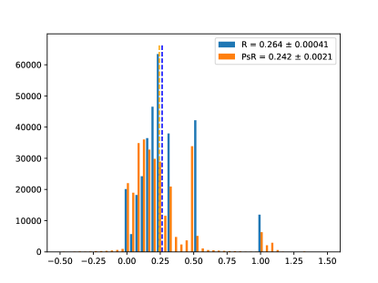
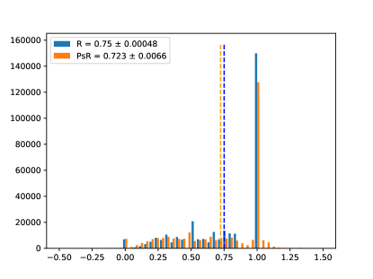
Figure 7: Histograms of propensity-scored (PsR) and vanilla recall (R) for top-1 (left) and top-5 (right) predictions for the AmazonCat-13K dataset for a DiSMEC model trained with a convex surrogate of the propensity-scored 0-1 loss. The y-axis denotes the number of examples in the test set for which the estimate falls into the corresponding bin. The errors have been calculated by boostrapping a 95 % confidence interval. The dashed vertical lines denote the mean.

C.2 Normalized BCE

In the main text, we claim that the low performance of unbiased training with normalized BCE in the high-regularization regime is due to bad local minima. Here we present supporting evidence.

Figure 8: Normalized Binary cross-entropy for different regularization strengths, evaluated on noisy training data, clean training data, and clean test data. Setting c’) corresponds to unbiased training with vanilla pre-training.

As shown in Figure 8, the low performance is caused by high loss on training data (dashed lines) as opposed to generalization. However, for training with vanilla loss b), the loss on noisy training data (i.e. the unbiased estimate computed on noisy training data) is much lower than for training with the unbiased loss c), where we directly try to optimize this quantity. There are two possible explanations for this behaviour: Either the switch to the unbiased loss shifts the balance of loss to regularizer such that the regularizer attains much more weight overall, and thus results in less optimization for the loss, or the optimization procedure gets stuck in a local minimum.

These two causes can be distinguished by an experiment where the initial weights are chosen by pre-training with vanilla loss for ten epochs. If the reason for the bad performance were the regularization trade-off, then the following 20 epochs of unbiased training would increase the training loss until the trade-off is reached. On the other hand, if the reason were local minima, then starting out close to a known "good" minimum would result in converging to that minimum.

Figure 8 exhibits the behaviour of the second case, thus validating the local-minima hypothesis.

References

- Agrawal et al. (2013) Rahul Agrawal, Archit Gupta, Yashoteja Prabhu, and Manik Varma. Multi-label learning with millions of labels: Recommending advertiser bid phrases for web pages. In Proceedings of the 22nd International Conference on World Wide Web, WWW ’13, page 13–24, New York, NY, USA, 2013. Association for Computing Machinery. ISBN 9781450320351. doi: 10.1145/2488388.2488391. URL https://doi.org/10.1145/2488388.2488391.
- Arpit et al. (2017) Devansh Arpit, Stanisław Jastrzębski, Nicolas Ballas, David Krueger, Emmanuel Bengio, Maxinder S. Kanwal, Tegan Maharaj, Asja Fischer, Aaron Courville, Yoshua Bengio, and Simon Lacoste-Julien. A Closer Look at Memorization in Deep Networks. In Doina Precup and Yee Whye Teh, editors, Proceedings of the 34th International Conference on Machine Learning, volume 70 of Proceedings of Machine Learning Research, pages 233–242. PMLR, 06–11 Aug 2017.
- Babbar and Schölkopf (2017) Rohit Babbar and Bernhard Schölkopf. Dismec: Distributed sparse machines for extreme multi-label classification. In WSDM, pages 721–729, 2017.
- Babbar and Schölkopf (2019) Rohit Babbar and Bernhard Schölkopf. Data scarcity, robustness and extreme multi-label classification. Machine Learning, 108(8):1329–1351, September 2019. ISSN 1573-0565. doi: 10.1007/s10994-019-05791-5. URL https://doi.org/10.1007/s10994-019-05791-5.
- Bhatia et al. (2016) Kush Bhatia, Kunal Dahiya, Himanshu Jain, Yashoteja Prabhu, and Manik Varma. The extreme classification repository: Multi-label datasets and code. http://manikvarma.org/downloads/XC/XMLRepository.html, 2016.
- Bucak et al. (2009) Serhat S Bucak, Pavan Kumar Mallapragada, Rong Jin, and Anil K Jain. Efficient multi-label ranking for multi-class learning: application to object recognition. In 2009 IEEE 12th International Conference on Computer Vision, pages 2098–2105. IEEE, 2009.
- Bucak et al. (2011) Serhat Selcuk Bucak, Rong Jin, and Anil K Jain. Multi-label learning with incomplete class assignments. In CVPR 2011, pages 2801–2808. IEEE, 2011.
- Chou et al. (2020) Yu-Ting Chou, Gang Niu, Hsuan-Tien Lin, and Masashi Sugiyama. Unbiased Risk Estimators Can Mislead: A Case Study of Learning with Complementary Labels. In International Conference on Machine Learning, pages 1929–1938. PMLR, November 2020. URL https://proceedings.mlr.press/v119/chou20a.html. ISSN: 2640-3498.
- Dahiya et al. (2021) K. Dahiya, A. Agarwal, D. Saini, K. Gururaj, J. Jiao, A. Singh, S. Agarwal, P. Kar, and M Varma. Siamesexml: Siamese networks meet extreme classifiers with 100m labels. In Proceedings of the International Conference on Machine Learning, July 2021.
- Dekel and Shamir (2010) Ofer Dekel and Ohad Shamir. Multiclass-multilabel classification with more classes than examples. In Proceedings of the Thirteenth International Conference on Artificial Intelligence and Statistics, pages 137–144, 2010.
- Deng et al. (2010) Jia Deng, Alexander C Berg, Kai Li, and Li Fei-Fei. What does classifying more than 10,000 image categories tell us? In ECCV, 2010.
- Du Plessis et al. (2015) Marthinus Du Plessis, Gang Niu, and Masashi Sugiyama. Convex formulation for learning from positive and unlabeled data. In International conference on machine learning, pages 1386–1394, 2015.
- Elkan and Noto (2008) Charles Elkan and Keith Noto. Learning classifiers from only positive and unlabeled data. In Proceedings of the 14th ACM SIGKDD international conference on Knowledge discovery and data mining, KDD ’08, pages 213–220, New York, NY, USA, August 2008. Association for Computing Machinery. ISBN 978-1-60558-193-4. doi: 10.1145/1401890.1401920. URL https://doi.org/10.1145/1401890.1401920.
- Ghosh et al. (2015) Aritra Ghosh, Naresh Manwani, and P. S. Sastry. Making risk minimization tolerant to label noise. Neurocomputing, 160:93–107, 2015. Publisher: Elsevier.
- Guo et al. (2019) Chuan Guo, Ali Mousavi, Xiang Wu, Daniel N. Holtmann-Rice, Satyen Kale, Sashank Reddi, and Sanjiv Kumar. Breaking the Glass Ceiling for Embedding-Based Classifiers for Large Output Spaces. Advances in Neural Information Processing Systems, 32, 2019. URL https://proceedings.neurips.cc/paper/2019/hash/78f7d96ea21ccae89a7b581295f34135-Abstract.html.
- Han et al. (2018) Bo Han, Quanming Yao, Xingrui Yu, Gang Niu, Miao Xu, Weihua Hu, Ivor Tsang, and Masashi Sugiyama. Co-teaching: Robust training of deep neural networks with extremely noisy labels. In S. Bengio, H. Wallach, H. Larochelle, K. Grauman, N. Cesa-Bianchi, and R. Garnett, editors, Advances in Neural Information Processing Systems, volume 31. Curran Associates, Inc., 2018. URL https://proceedings.neurips.cc/paper/2018/file/a19744e268754fb0148b017647355b7b-Paper.pdf.
- Jain et al. (2016) Himanshu Jain, Yashoteja Prabhu, and Manik Varma. Extreme multi-label loss functions for recommendation, tagging, ranking and other missing label applications. In KDD, August 2016.
- Jain et al. (2019) Himanshu Jain, Venkatesh Balasubramanian, Bhanu Chunduri, and Manik Varma. Slice: Scalable linear extreme classifiers trained on 100 million labels for related searches. In WSDM, pages 528–536, 2019.
- Jiang et al. (2018) Lu Jiang, Zhengyuan Zhou, Thomas Leung, Li-Jia Li, and Li Fei-Fei. MentorNet: Learning data-driven curriculum for very deep neural networks on corrupted labels. In Jennifer Dy and Andreas Krause, editors, Proceedings of the 35th International Conference on Machine Learning, volume 80 of Proceedings of Machine Learning Research, pages 2304–2313. PMLR, 10–15 Jul 2018. URL https://proceedings.mlr.press/v80/jiang18c.html.
- Kingma and Ba (2017) Diederik P. Kingma and Jimmy Ba. Adam: A method for stochastic optimization, 2017.
- Kiryo et al. (2017) Ryuichi Kiryo, Gang Niu, Marthinus C du Plessis, and Masashi Sugiyama. Positive-Unlabeled Learning with Non-Negative Risk Estimator. In I. Guyon, U. V. Luxburg, S. Bengio, H. Wallach, R. Fergus, S. Vishwanathan, and R. Garnett, editors, Advances in Neural Information Processing Systems 30, pages 1675–1685. Curran Associates, Inc., 2017. URL http://papers.nips.cc/paper/6765-positive-unlabeled-learning-with-non-negative-risk-estimator.pdf.
- Lapin et al. (2018) M. Lapin, M. Hein, and B. Schiele. Analysis and optimization of loss functions for multiclass, top-k, and multilabel classification. IEEE Transactions on Pattern Analysis and Machine Intelligence, 40(7):1533–1554, 2018. doi: 10.1109/TPAMI.2017.2751607.
- Menon et al. (2015) Aditya Menon, Brendan Van Rooyen, Cheng Soon Ong, and Bob Williamson. Learning from corrupted binary labels via class-probability estimation. In International Conference on Machine Learning, pages 125–134, 2015.
- Menon et al. (2019) Aditya K. Menon, Ankit Singh Rawat, Sashank Reddi, and Sanjiv Kumar. Multilabel reductions: what is my loss optimising? Advances in Neural Information Processing Systems, 32, 2019. URL https://papers.nips.cc/paper/2019/hash/da647c549dde572c2c5edc4f5bef039c-Abstract.html.
- Mikolov et al. (2013) Tomas Mikolov, Kai Chen, Greg Corrado, and Jeffrey Dean. Efficient estimation of word representations in vector space. arXiv preprint arXiv:1301.3781, 2013.
- Mohri et al. (2018) Mehryar Mohri, Afshin Rostamizadeh, and Ameet Talwalkar. Foundations of machine learning. MIT press, 2018.
- Natarajan et al. (2017) Nagarajan Natarajan, Inderjit S. Dhillon, Pradeep Ravikumar, and Ambuj Tewari. Cost-sensitive learning with noisy labels. The Journal of Machine Learning Research, 18(1):5666–5698, 2017. Publisher: JMLR. org.
- Partalas et al. (2015) Ioannis Partalas, Aris Kosmopoulos, Nicolas Baskiotis, Thierry Artieres, George Paliouras, Eric Gaussier, Ion Androutsopoulos, Massih-Reza Amini, and Patrick Galinari. Lshtc: A benchmark for large-scale text classification. arXiv preprint arXiv:1503.08581, 2015.
- Prabhu and Varma (2014) Yashoteja Prabhu and Manik Varma. Fastxml: A fast, accurate and stable tree-classifier for extreme multi-label learning. In KDD, pages 263–272. ACM, 2014.
- Qaraei et al. (2021) Mohammadreza Qaraei, Erik Schultheis, Priyanshu Gupta, and Rohit Babbar. Convex Surrogates for Unbiased Loss Functions in Extreme Classification With Missing Labels. In Proceedings of the Web Conference 2021, pages 3711–3720, Ljubljana Slovenia, April 2021. ACM. ISBN 978-1-4503-8312-7. doi: 10.1145/3442381.3450139. URL https://dl.acm.org/doi/10.1145/3442381.3450139.
- Shalev-Shwartz and Ben-David (2014) Shai Shalev-Shwartz and Shai Ben-David. Understanding machine learning: From theory to algorithms. Cambridge university press, 2014.
- Van Rooyen and Williamson (2017) Brendan Van Rooyen and Robert C. Williamson. A theory of learning with corrupted labels. 18(1):8501–8550, 2017. ISSN 1532-4435.
- Wydmuch et al. (2021) Marek Wydmuch, Kalina Jasinska-Kobus, Rohit Babbar, and Krzysztof Dembczynski. Propensity-Scored Probabilistic Label Trees, page 2252–2256. Association for Computing Machinery, New York, NY, USA, 2021. ISBN 9781450380379. URL https://doi.org/10.1145/3404835.3463084.
- You et al. (2019) Ronghui You, Zihan Zhang, Ziye Wang, Suyang Dai, Hiroshi Mamitsuka, and Shanfeng Zhu. Attentionxml: Label tree-based attention-aware deep model for high-performance extreme multi-label text classification. In H. Wallach, H. Larochelle, A. Beygelzimer, F. d'Alché-Buc, E. Fox, and R. Garnett, editors, Advances in Neural Information Processing Systems, volume 32. Curran Associates, Inc., 2019. URL https://proceedings.neurips.cc/paper/2019/file/9e6a921fbc428b5638b3986e365d4f21-Paper.pdf.
- Yu et al. (2014) Hsiang-Fu Yu, Prateek Jain, Purushottam Kar, and Inderjit Dhillon. Large-scale multi-label learning with missing labels. In International conference on machine learning, pages 593–601, 2014.
- Zheng et al. (2020) Songzhu Zheng, Pengxiang Wu, Aman Goswami, Mayank Goswami, Dimitris Metaxas, and Chao Chen. Error-bounded correction of noisy labels. In International Conference on Machine Learning, pages 11447–11457. PMLR, 2020.