Anisotropy of the proton kinetic energy as a tool for capturing structural transition in nanoconfined H₂O

Abstract

The proton dynamics of a 2D water monolayer confined inside a graphene slit pore is studied in Cartesian and molecular frames of reference using molecular dynamics simulations. The vibrational density of states of the proton was calculated versus temperature and was further used to deduce the mean kinetic energy of the hydrogen atoms, Ke(H), in both frames of reference. The directional components of Ke(H) are in good agreement with experimental observations for bulk as well as nanoconfined water. Nonetheless, while in the molecular frame of reference the effect of temperature on the anisotropy ratios of Ke(H) (the ratio between its directional components) are practically invariant between the 2D and 3D cases, those in the Cartesian frame of reference reveal a rather notable reduction across 200K, indicating the occurrence of an order-disorder transition. This result is further supported by the calculated entropy and enthalpy of the confined water molecules. Overall it is shown that Ke(H) anisotropy ratios may serve as a valuable order parameter for detecting structural transformations in hydrogen bonds containing molecular systems.

Water in confined geometries exhibit intriguing behaviors, much different from the ordinary bulk, hence studies of nanoconfined water provide valuable information regarding the physico-chemical nature of water dynamics, e.g. freezingDavid2019 , fluid organizationMochizuki2015 ; Koga2001 ; Algara2015 , mobilityHolt2006 ; Tunuguntla2017 ; Secchi2016 ; Mukherjee2007 ; Bonthuis2011 ; Naskar2020 and structural and dynamical transitionsNoon2002 ; Bai2006 ; Nomura2017 ; Majumdar2021 ; Joseph2008 . Structural transitions of confined water strongly depend on the nature and scale of confinementShiomi2007 ; Chakraborty2017 ; Mukherjee2008 . An interesting feature of confinement that receives a detailed attention in recent years, regards the fluid-solid interface, with the goal of understanding how the hydrophobicity and hydrophilicity of the confining lattice surface affects the structure and dynamics of guest water moleculesSchlaich2016 ; kayal2015 ; Lupi2014 . An exemplifying and well-studied example is water inside single wall carbon nanotubes (SWCNTs)Mochizuki2015 ; Whitby2008 ; Falk2010 .

Deep inelastic neutron scattering (DINS) is an exclusive experimental technique which is extensively used to explore proton dynamics in hydrogen bonds (HBs) containing systems. It allows for probing the dynamics of protons, as well as possible related nuclear (NQEs) and competing (CQEs) quantum effects, via a measurement of the proton momentum distribution and hence of its mean kinetic energy, Ke(H). This parameter was proved to be a fairly sensitive probe of H-dynamics, which by itself is dominated by the way the HBs network into three or reduced (two and one) dimensional phases. Up until now, the accumulated DINS findings suggest that when water is confined in 3D spaces of effective pore diameter less than 20Å, Ke(H) assumes anomalous values compared to those occurring in ice and liquid bulksReiter2012 ; Kolesnikov2016 ; Senesi2007 ; Pantalei2011 . In one of the DINS studies an attempt was made to probe the effect of 2D confinement on the H-dynamics in liquid (293K) and ice (20K), both confined between 12Å separated hydrophilic surfaces of graphene oxide sponges (GOs) at ambient pressureRomanelli2015 ; Andreani2017 . However, the measured Ke(H) values [summarized in Table 1] did not reveal any evidence of Ke(H) anomaly as compared to regular bulk water phasesColognesi2011 ; Finkelstein2014 ; Flammini2012 ; Andreani2013 . Note that for bulk water, the value of Ke(H) remains practically constant between 5K and 300K due to the dominance of the zero point value of Ke(H) in waterFinkelstein2014 .

The neutron scattered intensities in DINS experiments were also used to resolve the three Cartesian components of Ke(H), i.e. those along and perpendicular to the OH bond direction in 2D confined H₂O moleculesRomanelli2015 . It was found that the directional components of Ke(H) show a similar anisotropy as those previously reported for bulk iceFlammini2012 and waterAndreani2013 in the molecular frame of reference. The existing data is summarized in Table 1 with the orthogonal directions in the molecular frame of reference defined in Fig. 1(c).

In recent years, the partial vibrational density of states (pVDOS) approach was utilized for studying proton dynamics in various H containing systemsFlammini2012 ; Senesi2013 ; Pietropaolo2009 ; Andreani2016 ; Moid2020 , and is applied here for studying proton dynamics in nanoconfined water under 2D topology.

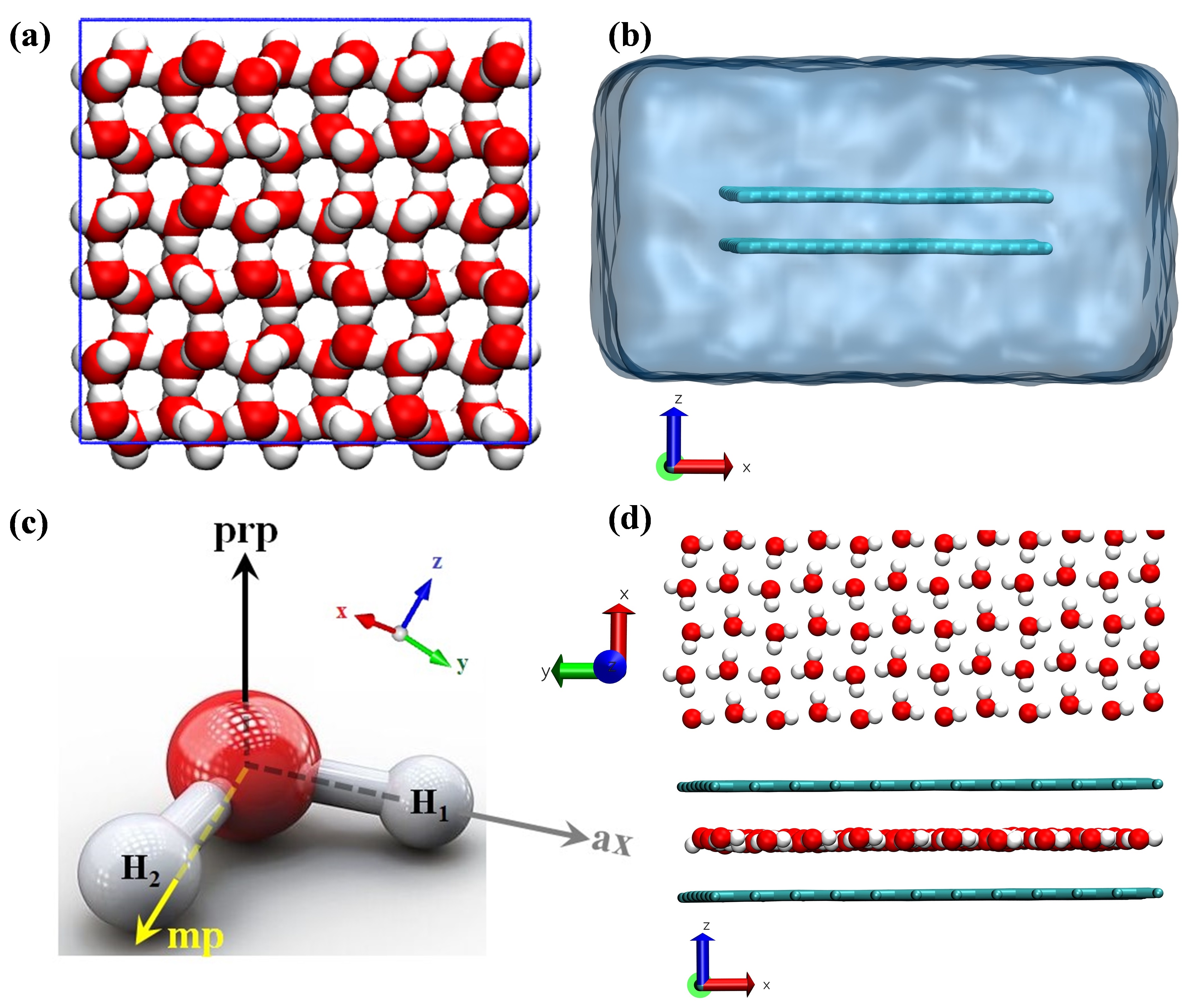
Figure 1: The initial structure of a 3D hexagonal bulk ice (a) and of 2D square ice confined inside a graphene slit-pore (b). Red and white colors denote oxygen and hydrogen atoms respectively. Gray lines and cyan background in (b) denote the graphene sheet and the water bath respectively. (c) the H₂O molecular frame of reference, as defined for an arbitrary orientation of a water molecule relative to the Cartesian frame of reference: ax (grey) is directed along one of the OH bonds, mp (yellow) lays in the H₂O molecular plane but extends normal to ax, and prp (black) is perpendicular to the H₂O plane. The relative orientations of the sandwiched ice monolayer and the confining graphene layers is given in (d). Note that in the simulation the Cartesian directions are fixed whereas those of the molecular frame of reference are updated with time according to the reorientation of molecules during the simulation.

Using this approach, we computed Ke(H) in two coordinate system, namely the Cartesian and Molecular frames of reference. To simulate the directional components of Ke(H) in any of the above coordinate system, we start by constructing the kinetic energy tensor whose principal components determine the kinetic energy values along the orthogonal direction of that coordinate system[see Appendix 1 for details]. For the simulation of both bulk and nanoconfined water phases, the flexible TIP4P-2005 water modelAbascal2005 ; Gonzalez2011 was utilized. For the 2D ice structureAlgara2015 ; Mario2015 ; Pascal2019 , simulations were performed using a 4x4 nm² graphene nanoslit pore of a 6.8 Å separation distance, embedded in a water bath [see Appendix 2 for further details of the simulation].

The upper panel of Fig. 2 depicts a total (spatial averaged) H-VDOS of an arbitrary H atom at 5 K, illustrating the typical pVDOS spectra used to deduce the temperature dependence of Ke(H) in bulk ice. Also shown in the lower panels of Fig. 2 are the directional VDOS profiles, computed for the H1 proton in a single H₂O in bulk ice at 5 K. The VDOS profiles were calculated for all water molecules composing the 3D and 2D model systems and then utilized to deduce the average total and directional Ke(H) values versus temperature. The temperature dependence of the directional Ke(H) values is presented in Fig. 3b.

We first note in the 3D bulk (solid lines in Fig. 3a) all directional Ke(H) components practically have the same value irrespective of the temperature, which well accords with the fact that on average, in bulk water phases, the H₂O molecules are isotropically oriented. In clear contrast, however, for the 2D confined water monolayer (dashed lines in Fig. 3a), marked differences are noted between the Ke(H) components along the (z) direction and perpendicular to it (x,y). Moreover, the two ”in-plane” monolayer components, Ke_x(H) and Ke_y(H), practically show the same values irrespective of the temperature due to the isotropy of the H₂O planes along the (x,y) plane, whereas those along the confining (”out-of-plane”) direction, Ke_z(H), show far much lower values. Also, the in-plane and out-of-plane Ke(H) components reveal an anti correlated, or mirror image behavior [Fig. 3(a)]. The isotropy, which leads to similar Ke(H) values along the X and Y directions, can be easily understood if one considers that the H₂O molecules composing the 2D monolayer, lay rather flat with respect to the graphene surface and on average, with no preferable in-plane orientation.

Table 1: Calculated and measured Ke(H) components in the molecular frame of reference of water under 3D (bulk) and 2D (H₂O@GOs) topologies. The ax, prp, mp directions with respect to the water molecule are defined in Fig. 1 and accord with those of Refs. Finkelstein2019 and Romanelli2015 . Ke_tot(H) is the algebraic sum over the three directional components. PIMD, INS and SE stand for the path integral molecular dynamics calculation, inelastic neutron scattering, and the semi empirical approach respectively. The SE values of the 271 solid 293 K liquid were calculated using the formulation presented in the supporting information of Ref. Parmentier2015 and by utilizing the structural and spectroscopic parameters of liquid water.

	3D								2D
	Ice						Liquid		H2O@GOs
Ke(H)	271K						285K	293K	20K	293K
	Calc.				Exp.		Exp.	Calc.	Exp.
	DFT	SE		PIMD	DINS	DINS	DINS	SE	DINS
		INS	Present
prp	30.9	21.6 $\pm$ 0.3	23 $\pm$ 3	24.2	28 $\pm$ 2	28.9 $\pm$ 2	18.3 $\pm$ 2	17.7 $\pm$ 3	26 $\pm$ 7	24 $\pm$ 6
mp	37.4	34.4 $\pm$ 1.2	36 $\pm$ 3	31.8	38 $\pm$ 5	38.1 $\pm$ 3	51.8 $\pm$ 4	38.9 $\pm$ 3	45 $\pm$ 9	45 $\pm$ 9
ax	87.7	98.8 $\pm$ 1.2	93 $\pm$ 3	99.5	91 $\pm$ 5	86.7 $\pm$ 3	83.8 $\pm$ 3	99.8 $\pm$ 3	84 $\pm$ 12	86 $\pm$ 12
Ketot(H)	156	154 $\pm$ 2	152 $\pm$ 5	155.5	157 $\pm$ 2	153.7 $\pm$ 2	153.9 $\pm$ 3	156.4 $\pm$ 5	154.9 $\pm$ 2	156.1 $\pm$ 2

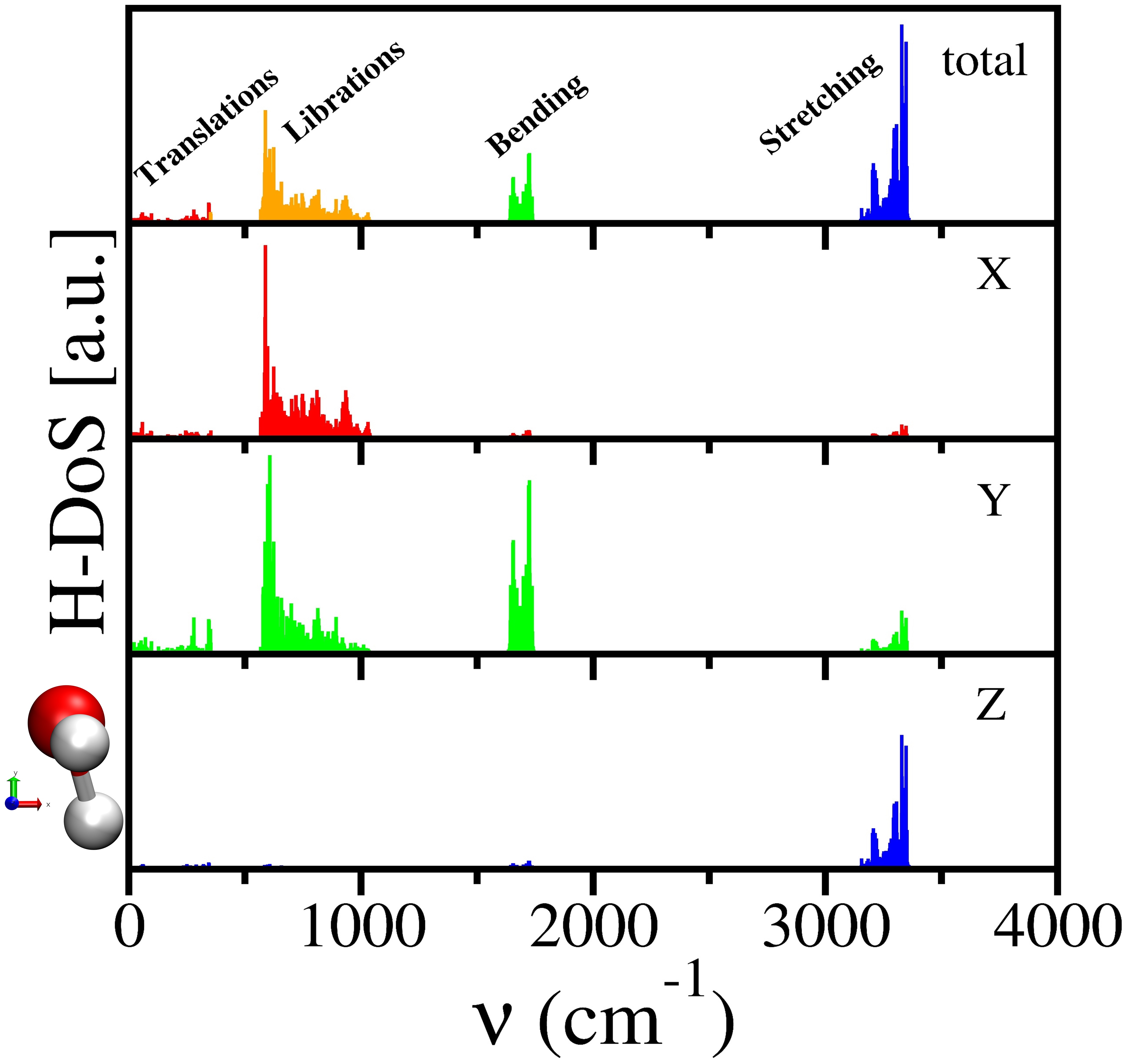
Figure 2: The upper panel depict the total H-VDOS resulting from a 500ps trajectory, computed for bulk ice at 5 K. The frequency bands at $\sim$[0-350] cm^-1 (red) and $\sim$[350-1250] cm^-1 (orange) comprise the lattice modes of translation and libration repectively. The peaks centered around $\sim$1700 (green) and 3300 (blue) cm^-1 arise from the molecular HOH bending and two OH stretching modes. The lower panels correspond to the computed projections in the molecular frame of reference of the H1-VDOS of an arbitrary H₂O molecule in bulk ice at 5K. Its individual orientation is depicted on the left. The noticeable differences between the three directional components of the H-VDOS illustrate the strong anisotropy of Ke(H) occurring in the molecular frame of reference.

It is also interesting to note that the 2D case reveals a phase transition occurring across the $\sim$ [170K-230K] temperature range. This is nicely reflected also by the instantaneous snapshots of the system at 170 K and 230 K [Fig. 3(b)] that illustrate a order-disorder transition. To characterise this transition, we computed the entropy and enthalpylin2003two ; lin2010two of the confined water, both characterized by a clear jump at 200 K. These jumps reveal a first order phase transition of the water molecules inside the graphene nanoporekumar2018 . Furthermore, the calculated water density inside the graphene nanopore and number of HBs per H₂O molecule versus temperature [Fig. 3(b)], are also both in accordance with a order-disorder phase transition around 200 K. While the number of HBs per H₂O is constant up to 170 K, it decreases rather sharply above that temperature. In order to quantify the structural changes across the transition, the calculation was supplemented with that of the radial distribution function at 170 and 230 K [Fig. 3(c)], showing a loss of ordering above 170 K. All in all, we quantified this transition as a first-order phase transition.

It is interesting to note that this transition is also captured by the variation in the kinetic energy tensor which changes upon confinement, depending on the order of confinement as well as on the dimension and nature of the confining geometry.Chakraborty2017 ; kumar2018 ; de2012 ; xu2011 The alteration in the kinetic energy tensor reflects a changed in the proton dynamics of the confined H₂O. In particular, it is seen in Fig. 3(a) that while the directional components of Ke(H) in the case of the 3D bulk possess fairly equal magnitudes and monotonically evolve with temperature, those in the 2D case noticeably differ in magnitude and are accompanied by step like abruptions across the phase transition temperature. The findings of Fig. 3 hint for an insightful way to capture the dynamics, namely to look at the evolution of the Ke(H) anisotropy versus temperature in both Cartesian and molecular frames of reference. In doing so we refer to three Ke(H) anisotropy ratios. The first one, in the Cartesian frame of reference, is of more relevance to the case of the lower dimensionality, and is defined [see Fig. 4] as the ratio between the average in-plane, K_a (H)=(Ke_x (H)+Ke_y (H))/2, and out of plane, K_c (H)=Ke_z (H), components. It evaluates the ratio between the average projections of Ke(H) along and perpendicular to the confining plane (z = constant). Hence, for the monolayer water that lays parallel to the graphene planes, a noticeable anisotropy may be expected, and moreover, any significant modification of the anisotropy ratio may suggest the occurrence of a structural reordering in the monolayer. In contrast, for the 3D case one may expect a practical isotropy, namely a unity ratio. The above is nicely evident by the red data points in Fig. 4 where K_a(H)/K_c(H) is nearly unity across the whole temperature range for the 3D case [Fig 4(a)], while exhibiting a rich temperature dependence in the confined case [Fig. 4(b)]. The temperature effect on the anisotropy ratio in the 2D case [red square in Fig. 4(b)] is ”commenced” at 5K with a rather large value of $\sim$3.9, moderately decreasing to $\sim$3.1 at 170K, then steeply declines down to $\sim$1.7 at 230K, hence nicely accords with the above discussed phase transition, and again continuously, but moderately, falls down to $\sim$1.5 at room temperature (RT).

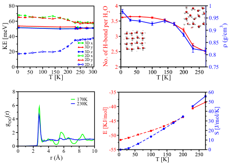
Figure 3: (a) Temperature dependence of the directional component of Ke(H) for the 2D and bulk cases. (b) Number of hydrogen bond per water molecules (red) and density of water inside the nanopore (blue) are constant up to 170 K and decreases rapidly above that temperature. (c) Oxygen-Oxygen 2D radial distribution function of water confined inside graphene nanoslit. (d) Entropy (blue) and enthalpy (red) with varying temperature reveals discontinuity around 200 K.

The other two anisotropy ratios [circles and triangles in Fig. 4] are defined in the molecular frame of reference [see Fig. 1(c)] which provides a means to look for signatures of competing quantum effects in Ke(H) such as those reported by DINS to occur upon melting of heavy water.Romanelli2013 The first ratio is defined between K_ax(H), the component of Ke(H) along the OH bond, and K_prp(H), that along the normal to the H₂O plane. Similarly, the remaining anisotropy ratio is defined as that between K_ax(H) and K_mp(H), the component of Ke(H) that lays in the H₂O plane but directed normal to K_ax(H). A marked but rather similar K_ax(H)/K_prp(H) anisotropy [green curves in Figs. 4(a) and (b)] is noticed for the 3D and 2D cases, which accords with the fact that up to 300K the molecular structure is after all preserved regardless of the water phase. This ratio depicts in fact the difference between the OH bond strength and that corresponding to the motions of the proton out of the H₂O molecular plane. In either of the 2D and 3D cases, the average number of HBs per water molecule decreases with increasing temperature [Fig. 3(b)], increasing in turn the OH bond strength. At the same time, however, the translational and librational motions are gradually diminished due to increased out of plane thermal motions, therefore the anisotropy is overall depressed. Since the average number of HBs at any given temperature is smaller in the 2D water monolayer, the OH bonds are strengthened compared to the 3D case, which increases the K_ax of 2D confined water compared to the bulk phase. As a result, the K_ax(H)/K_prp(H) anisotropy in the molecular frame of reference in the 2D case is relatively higher compared to the 3D bulk [Fig 4]. The calculated values of the anisotropy ratios versus temperature are shown in Fig. 4.

Finally, the K_ax(H)/K_mp(H) ratio (blue curves in Fig. 4) increases between 5 K and 300 K as a gradual and monotonous function, from $\sim$1.7 to $\sim$2.2 and from $\sim$2.1 to $\sim$2.9, for the 2D [Fig. 4(b)] and bulk [Fig. 4(a)] cases respectively. Interestingly, the K_ax(H)/K_mp(H) curve of the 2D system intersects that of K_ax(H)/K_prp(H) at about the median temperature of the transition range [Fig. 4(b)] across which the phase transition is detected.

It would be interesting to validate the findings of Fig 4 against experiment, namely DINS results. Unfortunately the DINS reports on water phases provide the directional Ke(H) values only in the molecular frame of reference. Nonetheless, an indirect experimental evidence for the above may be obtained by accounting for a very recent DINS study which was focused on investigating the effective isotropy of the proton local potential in a biphenyl hydrocarbon.Finkelstein1999 As in biphenyl, here too, the anisotropy is gradually diminished as the number of water units increase on going from the confined case of a water monolayer to the 3D bulk. This scenario is clearly reflected in Fig 4 for the molecular frame of reference, where the anisotropy ratio is insensitive in the 3D case [Fig. 4(a)] to the solid liquid transition, while revealing a clear sensitivity in the 2D case for the order-disorder transition [Fig. 4(b)].

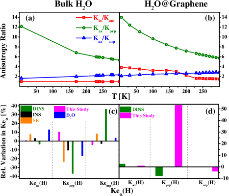
Figure 4: Anisotropy ratios of Ke(H) versus T for the 3D bulk (a) and the confined 2D monolayer (b), in the molecular (circles and triangles) and Cartesian (squares) frames of reference. The percentage variation of Ke(H) components across phase transitions occurring in bulk (c) and confined (d) water, as measured by DINS (green) and INS (black) and calculated by SE (orange) and in the present study (red). Left (c) and right (d) Y-axes values correspond to a relative increase and decrease in the Ke(H) component respectively. For bulk water, the values correspond to temperatures increasing from 250 to 300K (present calculation), 271 to 285K (INS and DINS) and 271 to 293K (SE). Similarly, for the confined case, the involved temperatures are: 140 to 230K (present study) and 20 to 293K (DINS). Blue bars correspond to DINS results of bulk D₂O (see text).Romanelli2013

Lastly, in former DINS studies the relative values of the directional Ke(H) components in the molecular frame of reference, as assumed by the protons across phase transitions of 2D and bulk water, were understood as signatures of competing quantum effects (CQEs) on Ke(H) upon the transition. It is thus of interest to examine also here how the directional components of Ke(H) in the molecular frame of reference vary across the phase transition in view of those reported by DINS for bulk water and water@Graphene. In the following discussion we also refer to the values presented in Table 1 which include SE calculations using INS dataAndreani2017 . The data points in Fig. 4 depict the percentage by which the Ke(H) components, for the molecular frame of reference in bulk water and in water@Graphene, vary across phase transition temperatures.

By reviewing the values of Figs. 4(c) and 4(d), no detectable distinction is noticed between the 3D and 2D systems, however the following three common features may be noted for the two cases. First, K_prp(H), the out of plane component of Ke(H), and K_ax(H), along the OH bond, seem to undergo the largest and smallest relative variations respectively across the phase transition. Second, in all cases at least one of the three components varies in opposite direction compared to the remaining two components. Lastly, the overall effect of these variations is of a compensating nature, namely such that impose a very small change in the total Ke(H) across the phase transition, hence the total Ke(H) reveals an overall picture of the same dynamics for the cases of the bulk and confined water. These particular features were previously observed by DINS measurements on bulk D₂O across the melting point.Romanelli2013 The directional components of the kinetic energy of the deutron, in the molecular frame of reference, were extracted in Ref. Romanelli2013 (as in Refs. Romanelli2015 ; Flammini2012 ; Andreani2013 ; Andreani2016 ) from the experimental momentum distribution by accounting for its measured profile as arising from the spherical average of an anisotropic Gaussian distribution. The [K_ax(D), K_prp(D), K_mp(D)] values (in meV units) were [48.1$\pm$3.4, 22.5$\pm$1.8, 37.4$\pm$2.5] and [54.2$\pm$2.4, 18.8$\pm$1.1, 38.6$\pm$2.5] at 274K (solid) and 280K (liquid) respectively. In comparison to Fig. 4(c), namely in terms of the percentage change going from the solid to the liquid phase in bulk H₂O, K_ax(D), K_prp(D) and K_mp(D) vary by $+$12.7%, -16.4% and +3.2% respectively [denoted by blue bars in Fig. 4(c)], with a corresponding total Ke(D) increment of ca. 3.3%, from 108.0$\pm$2.0 to 111.6$\pm$2.0 meV. This generic behaviour is generally used to assign the CQEs on Ke(H) upon melting,Romanelli2013 a behaviour which also has been observed in the present calculation.

In the present study, we explored the directional components of the ke(H) tensor for the cases of bulk water and a 2D water monolayer confined inside a graphene slit pore. We show that the flexible TIP4P-2005 model provides general good agreement with DINS measured values for bulk Ice-Ih and liquid over the entire studied temperature range between 5K and RT. More importantly, the calculated temperature effect on the directional Ke(H) tensor in water clearly reveals a significant change near 200 K which is indicative of a order-disorder phase transition. This transition is also reflected in the water density and average number of HBs per water molecule.

Interestingly, we also found that only a particular anisotropy ratio, namely that in the Cartesian frame of reference, acquires a sharp jump near the transition temperature, while that in the molecular frame of reference remains practically intact, that is, insensitive to the phase transition. Hence, we can conclude that depending on the geometry of confinement, Ke(H) anisotropy ratios may be used as a valuable choice of an order parameter for detecting order-disorder phase transitions.

I ACKNOWLEDGMENT

We acknowledge DST, India, for the computational support through TUECMS machine, IISc. We thank the DAE, India, and DST, India, for financial support. M.M. acknowledges the Councel of Sceintific and Industrial Research (CSIR), India, for financial support.

II Appendix

II.1 1. Theoretical Framework

To simulate the directional components of Ke(H) we start by constructing the kinetic energy tensor, whose principal components determine the kinetic energy values along the orthogonal direction of that coordinate system. The kinetic energy tensor in the Cartesian coordinate system may be expressed as:

$$\begin{pmatrix}Ke_{xx}&Ke_{xy}&Ke_{xz}\\ Ke_{yx}&Ke_{yy}&Ke_{yz}\\ Ke_{zx}&Ke_{zy}&Ke_{zz}\\ \end{pmatrix}$$

$Ke_{ij}$ denotes the atomic kinetic energy along that direction, with i and j standing for x,y or z direction.

Atomic kinetic energies in various phases can be calculated using different methods as discussed in detail in the literature.Finkelstein2019 ; Parmentier2015 Here, Ke(H) in condensed water phases is computed from the simulated pVDOS of the system, g${}^{H}_{ij}(n)$, i.e. the average projection of the total VDOS of the protons, by taking each vibrational state as a quantum harmonic oscillator using following equation:

$$Ke_{ij}(H)=\frac{\frac{3}{2}\int_{\nu_{\scaleobj{.6}0}}^{\nu_{\scaleobj{.6}f}}\text{g}^{H}_{ij}(\nu)\alpha(\nu,T)d\nu}{\int_{\nu_{\scaleobj{.6}0}}^{\nu_{\scaleobj{.6}f}}\text{g}^{H}_{ij}(\nu)d\nu}$$ (1)

where, g${}_{ij}^{H}$($\nu$) is the partial vibrational density of state (VDOS) of H atom with $\nu_{0}$ and $\nu_{f}$ frequency limits, and $\alpha$($\nu$,$T$) is the total energy of the quantum harmonic oscillator of frequency, $\nu$, at temperature $T$ given by

$$\alpha(\nu,T)=h\nu\left(\frac{1}{exp(\beta h\nu)-1}+\frac{1}{2}\right),$$ (2)

where, $\beta=\frac{1}{k_{B}T}$ and h is plank constant.

The partial VDOS, g${}_{ij}^{H}$($\nu$), (H-VDOS of atom H) is calculated in MD simulation using the mass weighted sum of atomic spectral densities:

$$\text{g}_{ij}^{H}(\nu)=\frac{2}{KT}\sum_{j=1}^{N}\sum_{k=1}^{3}m_{k}s_{ij}^{k}(\nu),$$ (3)

Where, m_k, is the atomic mass, k stands for the atom index for $k^{th}$ hydrogen in the system (e.g., 2N hydrogen atoms in a system comprising a total number of N water molecules). s${}_{ij}^{k}$($\nu$) is defined as the spectral density of the k^th H-atom, and is computed from the square of the Fourier transform of the corresponding velocities:

$$s_{ij}^{k}(\nu)=\lim_{\tau\to\infty}\frac{1}{2\tau}{\int_{-\tau}^{\tau}\int_{-\tau}^{\tau}V_{i}^{k}(t).V_{j}^{k}(t+t^{{}^{\prime}})dt^{{}^{\prime}}}e^{-\iota 2\pi\nu t}dt,$$ (4)

Where, V${}_{i}^{k}$ is the velocity of the $k^{th}$ H-atom along the $i^{th}$ direction at time $t$. The momentum-momentum correlation in two different directions does not correlate in a classical picture hence the off-diagonal term of the kinetic energy matrix becomes zero. Accordingly, the tensor can be rewritten in the form of a diagonalized tensor as follows:

$$\begin{pmatrix}Ke_{x}&0&0\\ 0&Ke_{y}&0\\ 0&0&Ke_{z}\\ \end{pmatrix}$$

$Ke_{i}$ the kinetic energy value along the i = x,y,z direction. Note that the spectral density of atoms can also be deduced from the velocity-velocity autocorrelation. One can write the total Ke(H) by summing over the directional components:

$$Ke(H)=Ke_{x}(H)+Ke_{y}(H)+Ke_{z}(H),$$ (5)

Integrating the VDOS over the whole frequency range will provide the total number of degrees of freedom of the system in the i^th direction: One can write the total Ke(H) by summing over the directional components:

$$\int_{0}^{\infty}g_{x}(\nu)d(\nu)=3N$$ (6)

II.2 2. Molecular Simulation details

We have performed MD simulation for hexagonal ice of 432 water molecules (3D case) and monolayer of water confined inside the graphene nano slit pore separated by 6.8 Å (2D case). For 3D water, we initiated the simulation at 5 K and 1 bar pressure with the initial hexagonal ice structures in the NPT ensemble. After 50 ns long NPT simulation, the final configuration from 5 K run was used as input to the next higher temperature of 100 K and so on. The simulations were performed at 100, 140, 170, 230, 240, 250, 270, 280, 300 K. NVT simulation was performed for 50 ns for each of the above mentioned temperature using the equilibrated configuration obtained in the NPT ensemble. The velocity-rescaleBussi2007 thermostat and Parrinello-Rahman barostat were used in NPT simulation with a temperature coupling constant of 1.3 ps and pressure coupling constant of 2 ps with the integration time step of 1 fs. Periodic boundary condition was used in all the three directions.

For 2D case, we initiated the simulation at 5 K and 1 bar pressure with the initial square ice structures between two graphene sheet separated by 6.8 Å, embedded in a 70 $\times$ 70 $\times$ 37 ų water bath. We performed 40 ns NPT simulation at 5, 30, 60, 100, 140, 170, 200, 230, 240, 250, 260, 270, 280, 290 and 300 K at 1 atm pressure in the NPT ensemble. After 40 ns equilibrium simulation in the NPT ensemble, we performed 10ns long NVT run. Throughout the simulation, graphene sheets were held fixed to its initial position using a harmonic restraint using a force constant of 1000 KJ/mol/nm² in each direction. We used Visual Molecular Dynamics (VMD) softwareHumphrey1996 to build graphene sheet of 4 $\times$ 4 nm² and xLeap module of AMBERCase2020 to solvate the nanopore using the TIP4P-2005 flexible water model.Abascal2005 ; Gonzalez2011

In each case, After NVT simulation, we performed another set of NVT simulation for 500 ps and save trajectory in every 2 femtosecond to compute density of state using velocity autocorrelation. A similar protocol was used in our earlier simulations of bulk and confined water.Moid2021 ; Raghav2015 ; Majumdar2021 The directional component of Ke(H) is averaged over at least 10 molecules for high temperature ($>$200 K) and up to 100 molecules at low temperature ($<$200 K).

References

- (1) R. O. David, C. Marcolli, J. Fahrni, Y. Qiu, Y. A. P. Sirkin, V. Molinero, F. Mahrt, D. Brühwiler, U. Lohmann, and Z. A. Kanji, “Pore condensation and freezing is responsible for ice formation below water saturation for porous particles,” Proceedings of the National Academy of Sciences, vol. 116, no. 17, pp. 8184–8189, 2019.
- (2) K. Mochizuki and K. Koga, “Solid- liquid critical behavior of water in nanopores,” Proceedings of the National Academy of Sciences, vol. 112, no. 27, pp. 8221–8226, 2015.
- (3) K. Koga, G. Gao, H. Tanaka, and X. C. Zeng, “Formation of ordered ice nanotubes inside carbon nanotubes,” Nature, vol. 412, no. 6849, pp. 802–805, 2001.
- (4) G. Algara-Siller, O. Lehtinen, F. Wang, R. R. Nair, U. Kaiser, H. Wu, A. K. Geim, and I. V. Grigorieva, “Square ice in graphene nanocapillaries,” Nature, vol. 519, no. 7544, pp. 443–445, 2015.
- (5) J. K. Holt, H. G. Park, Y. Wang, M. Stadermann, A. B. Artyukhin, C. P. Grigoropoulos, A. Noy, and O. Bakajin, “Fast mass transport through sub-2-nanometer carbon nanotubes,” Science, vol. 312, no. 5776, pp. 1034–1037, 2006.
- (6) R. H. Tunuguntla, R. Y. Henley, Y.-C. Yao, T. A. Pham, M. Wanunu, and A. Noy, “Enhanced water permeability and tunable ion selectivity in subnanometer carbon nanotube porins,” Science, vol. 357, no. 6353, pp. 792–796, 2017.
- (7) E. Secchi, S. Marbach, A. Niguès, D. Stein, A. Siria, and L. Bocquet, “Massive radius-dependent flow slippage in carbon nanotubes,” Nature, vol. 537, no. 7619, pp. 210–213, 2016.
- (8) B. Mukherjee, P. K. Maiti, C. Dasgupta, and A. Sood, “Strong correlations and fickian water diffusion in narrow carbon nanotubes,” The Journal of chemical physics, vol. 126, no. 12, p. 124704, 2007.
- (9) D. J. Bonthuis, K. F. Rinne, K. Falk, C. N. Kaplan, D. Horinek, A. N. Berker, L. Bocquet, and R. R. Netz, “Theory and simulations of water flow through carbon nanotubes: prospects and pitfalls,” Journal of Physics: Condensed Matter, vol. 23, no. 18, p. 184110, 2011.
- (10) S. Naskar, A. K. Sahoo, M. Moid, and P. K. Maiti, “Ultra-high permeable phenine nanotube membranes for water desalination,” arXiv preprint arXiv:2005.12145, 2020.
- (11) W. H. Noon, K. D. Ausman, R. E. Smalley, and J. Ma, “Helical ice-sheets inside carbon nanotubes in the physiological condition,” Chemical Physics Letters, vol. 355, no. 5-6, pp. 445–448, 2002.
- (12) J. Bai, J. Wang, and X. C. Zeng, “Multiwalled ice helixes and ice nanotubes,” Proceedings of the National Academy of Sciences, vol. 103, no. 52, pp. 19664–19667, 2006.
- (13) K. Nomura, T. Kaneko, J. Bai, J. S. Francisco, K. Yasuoka, and X. C. Zeng, “Evidence of low-density and high-density liquid phases and isochore end point for water confined to carbon nanotube,” Proceedings of the National Academy of Sciences, vol. 114, no. 16, pp. 4066–4071, 2017.
- (14) J. Majumdar, M. Moid, C. Dasgupta, and P. K. Maiti, “Dielectric profile and electromelting of a monolayer of water confined in graphene slit pore,” The Journal of Physical Chemistry B, 2021.
- (15) S. Joseph and N. Aluru, “Why are carbon nanotubes fast transporters of water?,” Nano letters, vol. 8, no. 2, pp. 452–458, 2008.
- (16) J. Shiomi, T. Kimura, and S. Maruyama, “Molecular dynamics of ice-nanotube formation inside carbon nanotubes,” The Journal of Physical Chemistry C, vol. 111, no. 33, pp. 12188–12193, 2007.
- (17) S. Chakraborty, H. Kumar, C. Dasgupta, and P. K. Maiti, “Confined water: structure, dynamics, and thermodynamics,” Accounts of chemical research, vol. 50, no. 9, pp. 2139–2146, 2017.
- (18) B. Mukherjee, P. K. Maiti, C. Dasgupta, and A. K. Sood, “Strongly anisotropic orientational relaxation of water molecules in narrow carbon nanotubes and nanorings,” Acs Nano, vol. 2, no. 6, pp. 1189–1196, 2008.
- (19) A. Schlaich, E. W. Knapp, and R. R. Netz, “Water dielectric effects in planar confinement,” Physical review letters, vol. 117, no. 4, p. 048001, 2016.
- (20) A. Kayal and A. Chandra, “Exploring the structure and dynamics of nano-confined water molecules using molecular dynamics simulations,” Molecular Simulation, vol. 41, no. 5-6, pp. 463–470, 2015.
- (21) L. Lupi and V. Molinero, “Does hydrophilicity of carbon particles improve their ice nucleation ability?,” The Journal of Physical Chemistry A, vol. 118, no. 35, pp. 7330–7337, 2014.
- (22) M. Whitby, L. Cagnon, M. Thanou, and N. Quirke, “Enhanced fluid flow through nanoscale carbon pipes,” Nano letters, vol. 8, no. 9, pp. 2632–2637, 2008.
- (23) K. Falk, F. Sedlmeier, L. Joly, R. R. Netz, and L. Bocquet, “Molecular origin of fast water transport in carbon nanotube membranes: superlubricity versus curvature dependent friction,” Nano letters, vol. 10, no. 10, pp. 4067–4073, 2010.
- (24) G. F. Reiter, A. I. Kolesnikov, S. J. Paddison, P. Platzman, A. P. Moravsky, M. A. Adams, and J. Mayers, “Evidence for an anomalous quantum state of protons in nanoconfined water,” Physical Review B, vol. 85, no. 4, p. 045403, 2012.
- (25) A. I. Kolesnikov, G. F. Reiter, N. Choudhury, T. R. Prisk, E. Mamontov, A. Podlesnyak, G. Ehlers, A. G. Seel, D. J. Wesolowski, and L. M. Anovitz, “Quantum tunneling of water in beryl: a new state of the water molecule,” Physical review letters, vol. 116, no. 16, p. 167802, 2016.
- (26) R. Senesi, A. Pietropaolo, A. Bocedi, S. Pagnotta, and F. Bruni, “Proton momentum distribution in a protein hydration shell,” Physical review letters, vol. 98, no. 13, p. 138102, 2007.
- (27) C. Pantalei, R. Senesi, C. Andreani, P. Sozzani, A. Comotti, S. Bracco, M. Beretta, P. E. Sokol, and G. Reiter, “Interaction of single water molecules with silanols in mesoporous silica,” Physical Chemistry Chemical Physics, vol. 13, no. 13, pp. 6022–6028, 2011.
- (28) G. Romanelli, R. Senesi, X. Zhang, K. P. Loh, and C. Andreani, “Probing the effects of 2d confinement on hydrogen dynamics in water and ice adsorbed in graphene oxide sponges,” Physical Chemistry Chemical Physics, vol. 17, no. 47, pp. 31680–31684, 2015.
- (29) C. Andreani, R. Senesi, M. Krzystyniak, G. Romanelli, and F. Fernandez-Alonso, “Atomic quantum dynamics in materials research,” in Experimental Methods in the Physical Sciences, vol. 49, pp. 403–457, Elsevier, 2017.
- (30) D. Colognesi, “Extraction of single-particle mean kinetic energy from macroscopic thermodynamic data,” Physica B: Condensed Matter, vol. 406, no. 14, pp. 2723–2730, 2011.
- (31) Y. Finkelstein and R. Moreh, “Temperature dependence of the proton kinetic energy in water between 5 and 673 k,” Chemical Physics, vol. 431, pp. 58–63, 2014.
- (32) D. Flammini, A. Pietropaolo, R. Senesi, C. Andreani, F. McBride, A. Hodgson, M. A. Adams, L. Lin, and R. Car, “Spherical momentum distribution of the protons in hexagonal ice from modeling of inelastic neutron scattering data,” The Journal of chemical physics, vol. 136, no. 2, p. 024504, 2012.
- (33) C. Andreani, G. Romanelli, and R. Senesi, “A combined ins and dins study of proton quantum dynamics of ice and water across the triple point and in the supercritical phase,” Chemical Physics, vol. 427, pp. 106–110, 2013.
- (34) R. Senesi, G. Romanelli, M. Adams, and C. Andreani, “Temperature dependence of the zero point kinetic energy in ice and water above room temperature,” Chemical Physics, vol. 427, pp. 111–116, 2013.
- (35) A. Pietropaolo, R. Senesi, C. Andreani, and J. Mayers, “Quantum effects in water: proton kinetic energy maxima in stable and supercooled liquid,” Brazilian Journal of Physics, vol. 39, pp. 318–321, 2009.
- (36) C. Andreani, G. Romanelli, and R. Senesi, “Direct measurements of quantum kinetic energy tensor in stable and metastable water near the triple point: An experimental benchmark,” The journal of physical chemistry letters, vol. 7, no. 12, pp. 2216–2220, 2016.
- (37) M. Moid, Y. Finkelstein, R. Moreh, and P. K. Maiti, “Microscopic study of proton kinetic energy anomaly for nanoconfined water,” The Journal of Physical Chemistry B, vol. 124, no. 1, pp. 190–198, 2019.
- (38) J. L. Abascal and C. Vega, “A general purpose model for the condensed phases of water: Tip4p/2005,” The Journal of chemical physics, vol. 123, no. 23, p. 234505, 2005.
- (39) M. A. González and J. L. Abascal, “A flexible model for water based on tip4p/2005,” The Journal of chemical physics, vol. 135, no. 22, p. 224516, 2011.
- (40) M. S. F. Mario, M. Neek-Amal, and F. Peeters, “Aa-stacked bilayer square ice between graphene layers,” Physical Review B, vol. 92, no. 24, p. 245428, 2015.
- (41) T. A. Pascal, C. P. Schwartz, K. V. Lawler, and D. Prendergast, “The purported square ice in bilayer graphene is a nanoscale, monolayer object,” The Journal of chemical physics, vol. 150, no. 23, p. 231101, 2019.
- (42) Y. Finkelstein, R. Moreh, F. Bianchini, and P. Vajeeston, “Anisotropy of the proton kinetic energy in ice ih,” Surface Science, vol. 679, pp. 174–179, 2019.
- (43) A. Parmentier, J. Shephard, G. Romanelli, R. Senesi, C. Salzmann, and C. Andreani, “Evolution of hydrogen dynamics in amorphous ice with density,” The journal of physical chemistry letters, vol. 6, no. 11, pp. 2038–2042, 2015.
- (44) Y. Finkelstein, R. Moreh, and O. Shahal, “Out-of-plane orientation of multilayer n2 films adsorbed on grafoil at 20 k,” Surface science, vol. 437, no. 3, pp. 265–276, 1999.
- (45) V. Kapil, A. Cuzzocrea, and M. Ceriotti, “Anisotropy of the proton momentum distribution in water,” The Journal of Physical Chemistry B, vol. 122, no. 22, pp. 6048–6054, 2018.
- (46) S.-T. Lin, M. Blanco, and W. A. Goddard III, “The two-phase model for calculating thermodynamic properties of liquids from molecular dynamics: Validation for the phase diagram of lennard-jones fluids,” The Journal of chemical physics, vol. 119, no. 22, pp. 11792–11805, 2003.
- (47) S.-T. Lin, P. K. Maiti, and W. A. Goddard III, “Two-phase thermodynamic model for efficient and accurate absolute entropy of water from molecular dynamics simulations,” The Journal of Physical Chemistry B, vol. 114, no. 24, pp. 8191–8198, 2010.
- (48) H. Kumar, C. Dasgupta, and P. K. Maiti, “Phase transition in monolayer water confined in janus nanopore,” Langmuir, vol. 34, no. 40, pp. 12199–12205, 2018.
- (49) E. de la Llave, V. Molinero, and D. A. Scherlis, “Role of confinement and surface affinity on filling mechanisms and sorption hysteresis of water in nanopores,” The Journal of Physical Chemistry C, vol. 116, no. 2, pp. 1833–1840, 2012.
- (50) L. Xu and V. Molinero, “Is there a liquid–liquid transition in confined water?,” The Journal of Physical Chemistry B, vol. 115, no. 48, pp. 14210–14216, 2011.
- (51) G. Romanelli, M. Ceriotti, D. E. Manolopoulos, C. Pantalei, R. Senesi, and C. Andreani, “Direct measurement of competing quantum effects on the kinetic energy of heavy water upon melting,” The Journal of Physical Chemistry Letters, vol. 4, no. 19, pp. 3251–3256, 2013.
- (52) G. Bussi, D. Donadio, and M. Parrinello, “Canonical sampling through velocity rescaling,” The Journal of chemical physics, vol. 126, no. 1, p. 014101, 2007.
- (53) W. Humphrey, A. Dalke, and K. Schulten, “Vmd: visual molecular dynamics,” Journal of molecular graphics, vol. 14, no. 1, pp. 33–38, 1996.
- (54) D. A. Case, K. Belfon, I. Ben-Shalom, S. R. Brozell, D. Cerutti, T. Cheatham, V. W. D. Cruzeiro, T. Darden, R. E. Duke, G. Giambasu, et al., “Amber 2020,” 2020.
- (55) M. Moid, S. Sastry, C. Dasgupta, T. A. Pascal, and P. K. Maiti, “Dimensionality dependence of the kauzmann temperature: A case study using bulk and confined water,” The Journal of Chemical Physics, vol. 154, no. 16, p. 164510, 2021.
- (56) N. Raghav, S. Chakraborty, and P. K. Maiti, “Molecular mechanism of water permeation in a helium impermeable graphene and graphene oxide membrane,” Physical Chemistry Chemical Physics, vol. 17, no. 32, pp. 20557–20562, 2015.