Nonlinear waves in a hot, viscous and non-extensive quark-gluon plasma

Abstract

The effects of the non-extensive statistics on the nonlinear propagation of perturbations have been studied within the scope of relativistic second order dissipative hydrodynamics with the non-extensive equation of state. We have shown that the equations, describing the propagation of nonlinear waves under such situation are KdV-type (Korteweg-De Vries). Apart from their preserved solitonic behaviour the dissipative nature of these waves are also observed. The waves with larger amplitude and width dissipate less and propagate faster and these waves deplete more for both smaller values of Tsallis parameter ($q$) and temperature ($T$) of the medium. For vanishingly small transport coefficients the nonlinear waves show breaking nature. These findings suggest that the nature of the propagation of the nonlinear waves may serve as a good probe to differentiate between the extensive and non-extensive thermodynamic nature of a fluid, such as the quark-gluon plasma, produced in relativistic nuclear collisions.

I Introduction

The propagation of perturbations in fluids have been widely used to unveil the thermodynamic state of the fluid. Depending on the magnitude of the perturbation, it has been categorized as linear Kirtskhalia (2016); Lick (1990) or nonlinear. If the magnitude of the perturbation is small compared to the average value of the corresponding physical quantities then it is categorized as linear. On the other hand, if the perturbation is comparable to the corresponding average value then it has to be treated as nonlinear. In the context of quark-gluon plasma (QGP), formed in relativistic heavy-ion collisions (RHICs) and Large Hadron Collider (LHC), the response of QGP to the perturbations may help in characterizing the medium. The locally equilibrated system of QGP responds to its high internal pressure by rapid expansion against the vacuum. The QGP formed in the violent collisions of nuclei cools due to expansion and subsequently transforms to hadronic matter via a cross over transition or through an intermediary coexisting phase (of QGP and hadrons) depending on the value of temperature ($T$) and baryonic chemical potential ($\mu$) attained in these collisions. When these hadrons cease to interact, their momenta get frozen to certain value and finally move freely to the detector. The momentum spectra of these detected hadrons are analyzed to understand the dynamics of the collisions. In addition to the hadrons, penetrating probes, such as photons and lepton pairs emanated from each space time point of the medium, are also detected to shed light on the early hot and dense phase of QGP Busza et al. (2018).

The pressure gradient in QGP can be anisotropic and the degree of anisotropy depends on the value of impact parameter of the collisions. An anisotropic interacting system of quarks and gluons created after the collisions will develop a pressure gradient of different magnitudes along different directions. This anisotropic pressure gradient will result in different expansion rate which in turn will induce anisotropy in momentum distribution of the hadrons originating from the system on hadronization. For the small initial spatial anisotropy, the produced momentum anisotropy could be interpreted as linear response to the initial spatial anisotropy. However, nonlinear effects will be crucial if the anisotropy in initial geometry is large due to collisions at large impact parameter. Moreover, quarks and gluons produced in the early stage of collision with high momenta, do not equilibrate but propagate as jets through the thermal medium created due to the rescattering of the low momentum quarks and gluons. These jets, while propagating, deposit energy in the medium Shuryak (2009); Betz (2009). If the magnitude of the energy density resulting from the jet-medium interaction is comparable to the energy density of the medium, then the effects of jet propagation on the medium needs to be treated as nonlinear. On the other hand, smaller value of the deposited energy density allows the study of the jet-medium interaction within the domain of linear response theory. The propagation of linear perturbations in QGP has been studied extensively by several authors Staig and Shuryak (2011a, b); Sarwar and Alam (2018); Rafiei and Javidan (2016); Hasanujjaman et al. (2020, 2021); Minami and Kunihiro (2010); Rahaman and Alam (2018). However, the nonlinear aspects of the perturbations in QGP have been studied only by a few authors Raha et al. (1985); Fowler et al. (1982); Raha and Weiner (1983); Hefter et al. (1985); Fogaça et al. (2010, 2014); Sarwar et al. (2021). In Refs. Raha et al. (1985); Fowler et al. (1982) the authors have considered the background medium to be an ideal fluid and found that the nature of perturbations is solitonic. Fogaca et. al. in Refs. Fogaça et al. (2010, 2014) went further and introduced the shear viscous effects in the medium and considered the perturbations up to second order. They too, found the solitonic nature of the perturbations. In these studies, the local equilibrium is treated within the scope of Gibbs-Boltzmann (GB) extensive distribution. However, particle spectra from small systems produced in $p+p$ collision are found to be well described by non-extensive equilibrium distribution suggested by Tsallis Tsallis (1988); Constantino (2009); Khachatryan et al. (2010); Acharya et al. (2018); Biro et al. (2009); Cleymans et al. (2013); Marques et al. (2015); Bhattacharyya et al. (2016a); Tripathy et al. (2016); Grigoryan (2017); Bhattacharyya et al. (2018); Azmi et al. (2020). In fact, the data is better reproduced Wong et al. (2015); Azmi and Cleymans (2015); Bhattacharyya et al. (2018); Cleymans and Worku (2012); Zheng and Zhu (2016) with Tsallis distribution than the GB distribution.

The appearance of the entropic index, $q\neq 1$ (also called non-extensive parameter) in Tsallis distribution is attributed to the local fluctuations in the system Wilk and Wlodarczyk (2000). It is important to recall at this point that, in the limit of $q\rightarrow 1$, the Tsallis distribution approaches the GB distribution. In principle, $q$ can be determined from the dynamics of the system. For some cases, like non-linear Fokker-Planck equation Tsallis and Bukman (1996), Boltzmann lattice model Boghosian et al. (2003), cold atoms in optical lattices Douglas et al. (2006) etc, the $q$ is known analytically in terms of microscopic or mesoscopic quantities. A relation between the entropic index $q$ and the basic parameters of the QCD has been established in Refs. Deppman et al. (2020a, b). Furthermore, it was shown that, this value of $q$ can be used to reproduce the transverse momentum spectra of hadrons produced in relativistic proton+proton collisions Deppman et al. (2020c). The value of $q$ for a many body system has been expressed in terms of the number of particles ($N$) as, $q=1+2N^{-1}/3$ and it was shown that, the two particle correlation becomes weaker as $N\rightarrow\infty$ i.e. when the system approaches the domain of molecular chaos Lima and Deppman (2020). This nicely depicts the importance of non-extensitivity of a system with finite number of particles and has relevance for system formed in high energy collisions of protons and nuclei. It has been shown in Ref. Wilk and Wlodarczyk (2000) that, in a system with fluctuating temperature zones, $q$ is related to the relative variance in temperature. The interplay between the parameter $q$ and the QCD dynamics has been studied in Refs. Rozynek and Wilk (2016); Rożynek and Wilk (2019). In relativistic nuclear collisions, the $q$ is treated as a parameter to fit the transverse momentum spectra of hadrons, which can in principle vary from 0 to $\infty$. However, for the phenomenological studies, the values of $q$ are generally greater than one and from the thermodynamic considerations it has an upper bound of 4/3 Bhattacharyya et al. (2016b). The descriptions of different experimental observables, which carry the effect of fluctuations, require $q\neq 1$ as argued in Refs. Wilk and Wlodarczyk (2000); Navarra et al. (2003, 2004); Biyajima et al. (2005, 2006); Wilk and Wlodarczyk (2002, 2009); Biro and Jakovac (2005). The value of $q$ varies with collision centrality, energy and system size Biyajima et al. (2005, 2006). It has been reported that the system size alone is not sufficient to explain the value of non-extensive parameter Deb et al. (2021).

Moreover, there are other observables advocated for choosing the non-extensive local thermal equilibrium. The system size dependence of quantum fluctuations has been studied theoretically in Refs. Das et al. (2020a, 2021a, 2021b). These fluctuations may be represented by the $q$ parameter. The particle spectra for small systems depends on the $q-$parameter. A similar situation may arise in bigger systems also as the spatial inhomogeneity created in such systems (produced in nuclear collisions) may contain some smaller zones of size similar to that of the entire system produced in a $p+p$ collision. This indicates that the local equilibrium of such systems may be considered to be non-extensive in nature. At this stage one should find out ways to distinguish whether non-extensive local equilibrium is the underlying nature or an extensive local equilibrium is the correct situation for the fluid. This requires investigations of the effect of non-extensivity on the response of the fluid to the perturbations.

To understand the distinguishing effects between the non-extensivity end extensivity in locally equilibrated fluid, one considers two aspects in this regard: a) the equation of state to be of a non-extensive form, and b) the fluid dynamic equations should also be of non-extensive type, i.e., to say that the fluid velocity must also be defined by taking into account the non-extensivity, which will clearly be different from the extensive one Osada and Wilk (2008).

Recently, the study of the propagation of non-linear waves has considered only the first order deviation from the extensive one, where the non-linear wave equation for first-order perturbation has been derived for the ideal fluid background with fixed thermodynamic quantities Bhattacharyya and Mukherjee (2020). In Ref. Bhattacharyya and Mukherjee (2020) breaking wave solution has been obtained for non-dissipative propagation of the nonlinear waves. However, it has been shown in Ref. Osada and Wilk (2008) that the ideal non-extensive hydrodynamics ($q$-hydrodynamics) is equivalent to extensive dissipative hydrodynamics ($d$-hydrodynamics). The corresponding dissipation should result from the non-extensive nature of fluid velocity field Osada and Wilk (2008). Therefore, even in ideal non-extensive background, one expects dissipative propagations of perturbations. Moreover, the local equilibrium leads to inherent gradients in the dynamical fields of fluid which leads to transport phenomenon. Therefore, it is important to investigate the dissipative propagation of nonlinear waves in the non-extensive background to understand the role of non-extensivity on the propagation of perturbations.

In this work, we proceed to investigate the propagation of nonlinear waves in QGP with non-extensive equation of state (EoS) and also with viscous-coefficients appearing from non-extensive nature of fluid. The aim is to find how the conclusion changes with the change in background (either extensive or non-extensive) and how $q$ affects the propagation of the nonlinear waves. The required equations for propagation (of nonlinear waves) are derived from Müller-Israel-Stewart (MIS) hydrodynamics and the order of perturbations are considered up to the second order.

The paper is organized as follows: in the next section, i.e in Sec. II, we derive the required equations for nonlinear waves from MIS theory with all the relevant transport coefficients. In the subsection II.A we discuss the MIS relativistic causal hydrodynamics. Subsection II.B contains the equation of motion of the fluid in (1+1) dimension. In subsection II.C, the non-linear equations governing the propagation of the perturbations through the fluid have been provided. The Equation of State (EoS) for the non-extensive fluid has been discussed in Sec. III. We present our results in Sec. IV and finally summarize the findings in Sec. V. Some of the mathematical equations and expressions are presented in Appendix A, B and C. We have used natural units ($\hbar=c=1,k_{B}=1$) and the signature of the Minkowski metric as: $g^{\mu\nu}=(1,-1,-1,-1)$.

II Framework of relativistic viscous hydrodynamics

In the following subsections we derive the equation of motions of non-linear perturbations propagating through a relativistic viscous fluid.

II.1 Hydrodynamic equations

The non-extensive version of ideal and first order dissipative hydrodynamics have been investigated in Ref. Osada and Wilk (2008) and Ref. Biro and Molnar (2012) respectively. It is found in Ref. Biro and Molnar (2012) that in the $q$-hydrodynamics, the main tensorial structure of energy momentum tensor remains same as the $d$-hydrodynamics whereas, changes appear only in thermodynamic quantities and EoS. Here we use this observation and derive the nonlinear wave equation from same tensorial structure of second order MIS theory, with thermodynamic quantities and equation of state from non-extensive thermodynamics. The fluid velocity field considered here has non-extensive nature.

Relativistic viscous hydrodynamics is a useful tool to describe the space-time evolution of the fluid created in relativistic heavy-ion collisions (RHICs). Depending on the magnitude of the expansion gradient, the order of the theory is being anticipated. Navier-Stokes (NS) theory deals with first-order gradients of hydrodynamic fields, usually designated as the first-order viscous hydrodynamics Eckart (1940); Landau and Lifshitz (1987). The solution of the NS equation is acausal and unstable. However, there are recently developed theories which shows that the first-order hydrodynamics can be stable as well as causal Bemfica et al. (2018, 2019, 2020); Kovtun (2019); Das et al. (2020b, c).

The second-order hydrodynamics takes into account the second order gradient in hydrodynamic fields and the relaxation effects were introduced to attain causality and stability. Several prescriptions of the second-order hydrodynamics can be found in Refs. Israel and Stewart (1979); Hiscock and Lindblom (1983); Koide et al. (2007); Romatschke (2010); Van and Biro (2008); Tsumura and Kunihiro (2010). In this work, the second-order MIS hydrodynamics Israel and Stewart (1979) is used to obtain the required evolution equations for nonlinear waves. For a fluid without conserved quantum number, the choice of Landau frame Landau and Lifshitz (1987) is very natural. However, Landau choice does not lead to a simple behaviour in the limit of low viscosities. But with the presence of high baryon number in a system, and with the presence of the other viscosities such as shear and bulk viscosities (which are not so low), our obvious choice of defining the fluid four-velocity is Eckart’s choice of frame Eckart (1940). Eckart frame represents a local rest frame where the net charge dissipation is vanishing but the energy dissipation is non-vanishing. Although we will use Eckart frame here, one may choose the Landau frame as well. In Eckart frame, the energy-momentum tensor (EMT) and particle current can be written as:

$$T^{\mu\nu} = \epsilon u^{\mu}u^{\nu}-p\Delta^{\mu\nu}+\Delta T^{\mu\nu}~{},$$ (1)

$$J^{\mu} = nu^{\mu}~{},$$ (2)

where, $\epsilon$ is the local energy density field, $u^{\mu}$ is the fluid four velocity, $p$ is the local pressure, and $\Delta T^{\mu\nu}$ is the correction to the EMT due to dissipation. The $u^{\mu}$ satisfies the condition $u^{\mu}u_{\mu}=1$, implying, $u^{\mu}\partial_{\nu}u_{\mu}=0$. The projection operator normal to $u^{\mu}$ is defined as $\Delta^{\mu\nu}=g^{\mu\nu}-u^{\mu}u^{\nu}$ such that, $\Delta^{\mu\nu}u_{\nu}=0$ and $\Delta^{\mu\nu}\Delta_{\mu\nu}=3$. The symmetric traceless projection normal to $u^{\mu}$ is defined as, $\Delta^{\mu\nu}_{\alpha\beta}=\frac{1}{2}(\Delta^{\nu}_{\alpha}\Delta^{\mu}_{\beta}+\Delta^{\mu}_{\alpha}\Delta^{\nu}_{\beta}-\frac{2}{3}\Delta^{\mu\nu}\Delta_{\alpha\beta})~{}$.

The dissipative part in $T^{\mu\nu}$ can be decomposed in terms of scalar, vector and tensor as:

$$\Delta T^{\mu\nu}=-\Pi\Delta^{\mu\nu}+q^{\mu}u^{\nu}+q^{\nu}u^{\mu}+\pi^{\mu\nu}~{}.$$ (3)

The energy momentum tensor in Eckart frame then reads as:

$$T^{\mu\nu}=\epsilon u^{\mu}u^{\nu}-(p+\Pi)\Delta^{\mu\nu}+q^{\mu}u^{\nu}+q^{\nu}u^{\mu}+\pi^{\mu\nu}~{}.$$ (4)

In the fluid rest frame, the vector and tensor form of dissipations are considered to be non-existent that is, $u_{\mu}q^{\mu}=0$, $u_{\mu}\pi^{\mu\nu}=0$. The scalar dissipation ($\Pi$) corresponds to the non-equilibrium pressure perturbation, which can not be made to relate to energy density using the EoS. It is related to volume expansion of the fluid, triggers small non-equilibrium perturbation, which tends to bring a new equilibrium state through the dissipative correction. The vector $q^{\mu}$ and the $\pi^{\mu\nu}$ correspond to dissipative energy flow and the shear stress tensor respectively. The relations between energy density, pressure and the dissipative fluxes and EMT are given by the following relations:

$$u_{\mu}T^{\mu\nu}u_{\nu} = \epsilon,\,\,\,\,q_{\alpha}=u_{\mu}T^{\mu\nu}\Delta_{\nu\alpha}=u_{\mu}\Delta T^{\mu\nu}\Delta_{\nu\alpha},$$

$$p+\Pi = -\frac{1}{3}\Delta_{\mu\nu}T^{\mu\nu},\,\,\,\,\Pi=-\frac{1}{3}\Delta_{\mu\nu}\Delta T^{\mu\nu},\,\,\,\,u_{\mu}\Delta T^{\mu\nu}=q^{\nu}~{}.$$ (5)

The equation of motion are obtained from the conservation of EMT and the net charge density (here the net baryon number) density as:

$$\partial_{\mu}T^{\mu\nu} = 0~{},$$ (6)

$$\partial_{\mu}J^{\mu} = 0~{}.$$ (7)

The dissipative fluxes Israel and Stewart (1979) are given by,

$$\Pi = -\frac{1}{3}\zeta\Big{[}\partial_{\mu}u^{\mu}+\beta_{0}D\Pi-\tilde{\alpha_{0}}\partial_{\mu}q^{\mu}\Big{]}~{},$$ (8)

$$\pi^{\lambda\mu} = -2\eta\Delta^{\lambda\mu\alpha\beta}\Big{[}\partial_{\alpha}u_{\beta}+\beta_{2}D\pi_{\alpha\beta}-\tilde{\alpha_{1}}\partial_{\alpha}q_{\beta}\Big{]}~{},$$ (9)

$$q^{\lambda} = -\kappa T\Delta^{\lambda\mu}\Big{[}\frac{1}{T}\partial_{\mu}T+Du_{\mu}+\tilde{\beta_{1}}D{q_{\mu}}-\tilde{\alpha_{0}}\partial_{\mu}\Pi-\tilde{\alpha_{1}}\partial_{\nu}\pi^{\nu}_{\mu}~{}.\Big{]}$$ (10)

Here, $\eta$, $\zeta$, $\kappa$ are the coefficient of shear viscosity, bulk viscosity and thermal conductivity respectively. $D\equiv u^{\mu}\partial_{\mu}$, is the co-moving derivative and in the local rest frame (LRF) it represents the time derivative, $D\Pi=\dot{\Pi}$. The quantities, $\beta_{0},\tilde{\beta_{1}},\beta_{2}$ are relaxation coefficients, $\tilde{\alpha_{0}}$ and $\tilde{\alpha_{1}}$ are coupling coefficients. The $\beta_{0},\tilde{\beta_{1}}$ and $\beta_{2}$ are also related to the relaxation time scale as Muronga (2004, 2002):

$$\tau_{\Pi}=\zeta\beta_{0},\,\,\,\,\tau_{q}=\kappa T\beta_{1},\,\,\,\,\tau_{\pi}=2\eta\beta_{2}$$ (11)

And the coupling coefficients are related to the relaxation lengths, which couple to heat flux, and bulk pressure $(l_{q\Pi},l_{\Pi q})$, the heat flux, and shear tensor $(l_{q\pi},l_{\pi q})$ by the following relation

$$l_{\Pi q}=\zeta\alpha_{0},\,\,\,\,l_{q\Pi}=\kappa T\alpha_{0},\,\,\,\,l_{q\pi}=\kappa T\alpha_{1},\,\,\,\,l_{\pi q}=2\eta\alpha_{1}~{}.$$ (12)

The expressions for relaxation and coupling coefficients are given in Appendix-A.

II.2 1-D flow equations

In this section the relevant equations are derived to study the propagation of nonlinear perturbation in a fluid in $(1+1)$ dimension. The evolution equations of energy density and fluid velocity are obtained from the Eqs.(6) and (7) by taking projection along the directions parallel and perpendicular to $u^{\mu}$ as:

$$D\epsilon=-(\epsilon+p)\theta+(\partial_{\mu}u_{\nu})\Delta T^{\nu\mu}-(\partial_{\mu}q^{\mu})~{},$$ (13)

$$(\epsilon+p)Du^{\alpha}=\Delta^{\alpha\mu}\partial_{\mu}-\Delta^{\alpha}_{\nu}\partial_{\mu}\Delta T^{\nu\mu}~{},$$ (14)

where, $u^{\mu}=(\gamma,\gamma v,0,0),\,\,\,\,\gamma=1/\sqrt{1-v^{2}}$ and

$$\theta = \partial_{\mu}u^{\mu}=v\gamma^{3}\frac{\partial v}{\partial t}+\gamma^{3}\frac{\partial v}{\partial x}~{},$$ (15)

$$\partial_{\mu}q^{\mu} = q^{x}\frac{\partial v}{\partial t}+v\frac{\partial q^{x}}{\partial t}+\frac{\partial q^{x}}{\partial x}~{}.$$ (16)

Here,

$$u_{\mu}q^{\nu}=0,\,\,\,u_{\mu}\pi^{\mu\nu}=0,\,\,\,g_{\mu\nu}\pi^{\mu\nu}=0,\,\,\,\pi^{xy}=\pi^{zx}=\pi^{yz}=0,\,\,\,\pi^{yy}=\pi^{zz}=\pi^{T}$$ (17)

which leads to,

$$\pi^{00}=v^{2}\pi^{xx},\,\,\,\pi^{xt}=\pi^{tx}=v^{2}\pi^{xx},\,\,\,\pi^{T}=\pi^{tx}=\frac{(v^{2}-1)}{2}\pi^{xx}~{},$$ (18)

and

$$q^{t}=vq^{x},\,\,\,q^{y}=q^{z}=q^{T}~{}.$$ (19)

Now from the energy-momentum conservation equations i.e from Eqs.(13), and (14), we get,

$$\gamma v\Big{(}\frac{\partial\epsilon}{\partial t}+\frac{\partial\epsilon}{\partial x}\Big{)}= \Big{[}(h+\Pi)v\gamma^{3}+v\gamma\pi^{xx}+q^{x}\}\frac{\partial v}{\partial t}\Big{]}$$ (20)

$$+\Big{[}(h+\Pi)\gamma^{3}+\gamma\pi^{xx}\Big{]}\frac{\partial v}{\partial x}+v\frac{\partial q^{x}}{\partial t}+\frac{\partial q^{x}}{\partial x},$$

$$\Big{[}(h+\Pi)v\gamma^{4}+v\gamma^{2}(1-2v^{2})v\pi^{xx}+\gamma^{3}(1+v^{2})vq^{x}\Big{]}\frac{\partial v}{\partial t}+\Big{[}(h+\Pi)v\gamma^{4}-\gamma^{2}v^{2}\pi^{xx}$$

$$+\gamma v(1+2\gamma^{2})q^{x}\Big{]}\frac{\partial v}{\partial x}=-v^{2}\Big{[}\gamma^{2}\frac{\partial p_{\zeta}}{\partial t}+\frac{\gamma^{2}}{v}\frac{\partial p_{\zeta}}{\partial x}+\frac{\partial\pi^{xx}}{\partial t}+\frac{1}{v}\frac{\partial\pi^{xx}}{\partial x}+\frac{\gamma}{v}\frac{\partial q^{x}}{\partial t}-\gamma\frac{\partial q^{x}}{\partial x}\Big{]}$$ (21)

where $h=\epsilon+p$ is the enthalpy density. We define $p+\Pi=p_{\zeta}$. The equation governing the net baryon number conservation reads,

$$\frac{\partial n}{\partial t}+v\frac{\partial n}{\partial x}=-n\gamma^{2}\Big{[}v\frac{\partial v}{\partial t}+\frac{\partial v}{\partial x}\Big{]}~{},$$ (22)

The other three equations originating from dissipative fluxes are given by the Eqs.(8), (9), and (10), which can be written as:

$$\Pi+\zeta\beta_{0}\Big{[}\gamma\frac{\partial\Pi}{\partial t}+v\frac{\partial\Pi}{\partial x}\Big{]} = -\zeta\Big{[}\{v\gamma^{3}-\alpha_{0}q^{x}\}\frac{\partial v}{\partial t}+\{\gamma^{3}\}\frac{\partial v}{\partial x}-\alpha_{0}v\frac{\partial q^{x}}{\partial t}-\alpha_{0}\frac{\partial q^{x}}{\partial x}\Big{]}~{},$$ (23)

$$q^{x}+\kappa T\beta_{1}\Big{[}\gamma\frac{\partial q^{x}}{\partial t}+v\frac{\partial q^{x}}{\partial x}\Big{]} = \kappa T\Big{[}\{-\gamma^{4}+\beta_{1}\gamma^{3}vq^{x}+\alpha_{1}(2-\gamma^{2})\pi^{xx}\}\frac{\partial v}{\partial t}+\{-v\gamma^{4}$$ (24)

$$+\beta_{1}\gamma^{3}v^{2}q^{x}-\alpha_{1}\gamma^{2}v\pi^{xx}\}\frac{\partial v}{\partial x}+\alpha_{1}v\frac{\partial\pi^{xx}}{\partial t}+\alpha_{1}\frac{\partial\pi^{xx}}{\partial x}$$

$$-\alpha_{0}v\gamma^{2}\frac{\partial\Pi}{\partial t}-\alpha_{0}\gamma^{2}\frac{\partial\Pi}{\partial x}+\frac{1}{T}v\gamma^{2}\frac{\partial T}{\partial t}+\frac{1}{T}\gamma^{2}\frac{\partial T}{\partial x}\Big{]}~{},$$

$$\pi^{xx}+\frac{4}{3}\eta\beta_{2}\Big{[}\gamma\frac{\partial\pi^{xx}}{\partial t}+v\frac{\partial\pi^{xx}}{\partial x}\Big{]} = \frac{4}{3}\eta\Big{[}\{\gamma^{5}+\alpha_{1}\gamma^{4}vq^{x}+2\beta_{2}\gamma^{3}\pi^{xx}\}\frac{\partial v}{\partial t}+\{\gamma^{5}+\alpha_{1}\gamma^{4}vq^{x}$$ (25)

$$+2\beta_{2}\gamma^{3}v^{2}\pi^{xx}\}\frac{\partial v}{\partial x}-\alpha_{1}\gamma^{2}v\frac{\partial q^{x}}{\partial t}-\alpha_{1}\gamma^{2}\frac{\partial q^{x}}{\partial x}]~{}.$$

II.3 Derivation of nonlinear wave equations

The above hydrodynamic equations from MIS causal theory is used to derive the nonlinear equations governing the motion of the perturbations in the fluid. We have adapted Reductive Perturbative Method (RPM) Washimi and Taniuti (1966); Davidson (1972); Leblond (2008); Kraenkel et al. (1995). To proceed further we need to define ‘stretched co-ordinates’ as,

$$X=\frac{\sigma^{1/2}}{L}(x-c_{s}t),\text{and}\hskip 11.38092ptY=\frac{\sigma^{3/2}}{L}(c_{s}t)~{},$$ (26)

where, $L$ is the characteristic length and $c_{s}$ is the speed of sound. Therefore, from the above equations we get

$$\frac{\partial}{\partial x}=\frac{\sigma^{1/2}}{L}\frac{\partial}{\partial X},\text{and}\hskip 11.38092pt\frac{\partial}{\partial t}=-c_{s}\frac{\sigma^{1/2}}{L}\frac{\partial}{\partial X}+c_{s}\frac{\sigma^{3/2}}{L}\frac{\partial}{\partial Y}~{},$$ (27)

where $\sigma$ is the expansion parameter. The coordinate $X$ is measured from the frame of propagating sound waves, whereas the $Y$ represents fast moving coordinate. The RPM technique is devised to preserve the structural form of the parent equation. Now we perform the simultaneous series expansion of hydrodynamic quantities in powers of $\sigma$ to get,

$$\hat{\epsilon} = \frac{\epsilon}{\epsilon_{0}}=1+\sigma\epsilon_{1}+\sigma^{2}\epsilon_{2}+\sigma^{3}\epsilon_{3}+...,\,\,\,\hat{p}=\frac{p}{p_{0}}=1+\sigma p_{1}+\sigma^{2}p_{2}+\sigma^{3}p_{3}+...,$$

$$\hat{v} = \frac{v}{c_{s}}=\sigma v_{1}+\sigma^{2}v_{2}+\sigma^{3}v_{3}+...,\,\,\,\,\,\,\,\,\,\,\,\,\hat{\Pi}=\frac{\Pi}{p_{0}}=\sigma\Pi_{1}+\sigma^{2}\Pi_{2}+\sigma^{3}\Pi_{3}+...,$$

$$\hat{q}^{x} = \frac{q^{x}}{\epsilon_{0}}=\sigma q^{x}_{1}+\sigma^{2}q^{x}_{2}+\sigma^{3}q^{x}_{3}+...,\,\,\,\,\,\,\,\hat{\pi}^{xx}=\frac{\pi^{xx}}{p_{0}}=\sigma\pi^{xx}_{1}+\sigma^{2}\pi^{xx}_{2}+\sigma^{3}\pi^{xx}_{3}+...$$ (28)

By collecting terms with different order of $\sigma$ from the perturbation series different types of equation like Breaking wave equation, Burgers equation or KdV equation, etc can be obtained Fogaça et al. (2010); Lick (1990); Bhattacharyya and Mukherjee (2020).

We rewrite the equations of motions (Eqs. 20, II.2, 22, 23, 24, 25) using Eqs. 27, 28 and collect terms with order upto $\sigma^{3}$ and finally revert from $(X,Y)\to(t,x)$ to get the following equations for the perturbation in the energy density ($\hat{\epsilon}$) as:

$$\frac{\partial\hat{\epsilon_{1}}}{\partial t}+\left[1+(1-c_{s}^{2})\frac{\epsilon_{0}}{\epsilon_{0}+p_{0}}\hat{\epsilon_{1}}\right]c_{s}\frac{\partial\hat{\epsilon_{1}}}{\partial x}-\left[\frac{1}{2(\epsilon_{0}+p_{0})}(\zeta+\frac{4}{3}\eta)\right]\frac{\partial^{2}\hat{\epsilon_{1}}}{\partial x^{2}}=0,$$ (29)

and

$$\frac{\partial\hat{\epsilon_{2}}}{\partial t}+\mathcal{S}_{1}\frac{\partial\hat{\epsilon_{2}}}{\partial x}+\mathcal{S}_{2}\frac{\partial\hat{\epsilon_{1}}}{\partial x}+\mathcal{S}_{3}\frac{\partial^{2}\hat{\epsilon_{1}}}{\partial x^{2}}+\mathcal{S}_{4}\frac{\partial^{3}\hat{\epsilon_{1}}}{\partial x^{3}}+\mathcal{S}_{5}\frac{\partial^{2}\hat{\epsilon_{2}}}{\partial x^{2}}=0~{}.$$ (30)

where $\hat{\epsilon_{i}}=\sigma^{i}\epsilon_{i}$ for $i=1,2,.....$. The coefficients $\mathcal{S}_{i}$’s for $i=1$ to $5$ are given in Appendix-B. Eqs. (29) and (30) have been solved to investigate the fate of the nonlinear waves propagating through a relativistic viscous and non-extensive fluid. The relevant EoS and the initial conditions required to solve these equations are discussed in section III and IV respectively.

III Tsallis MIT bag equation of state

We assume that the quarks and gluons in the viscous plasma medium follow the quantum Tsallis Fermionic ($F$) and Bosonic ($B$) single particle distributions given by Rahaman et al. (2021),

$$f_{Fq}=\frac{1}{\left[1+(q-1)\frac{E_{p}-\mu}{T}\right]^{\frac{q}{q-1}}+1}$$

$$f_{Bq}=\frac{1}{\left[1+(q-1)\frac{E_{p}-\mu}{T}\right]^{\frac{q}{q-1}}-1},$$ (31)

where, $E_{p}=\sqrt{p^{2}+m^{2}}$ is the single particle energy of a particle of mass $m$, $\mu$ is the (baryonic) chemical potential (assumed to be zero in the present work), $q$ is the Tsallis (non-extensitivity) parameter and $T$ is the Tsallis temperature. The $\epsilon$ and $p$ of a system of quarks and gluons in MIT bag model  Chodos et al. (1974) is given by,

$$\epsilon_{\mathrm{}} = \mathcal{B}+\epsilon_{B}+2\epsilon_{F},$$ (32)

$$P_{\mathrm{}} = -\mathcal{B}+P_{B}+2P_{F},$$ (33)

where $\mathcal{B}$ is the bag constant ($\mathcal{B}^{1/4}=200$ MeV). The $\epsilon_{i}$ and $P_{i}$ are given by,

$$\epsilon_{i}=g\int\frac{d^{3}p}{(2\pi)^{3}}E_{p}f_{iq},~{}\ \ \ \ P_{i}=g\int\frac{d^{3}p}{(2\pi)^{3}}\frac{p^{2}}{3E_{p}}f_{iq},$$ (34)

where $g$ is the degeneracy factor and $i=B,F$.

The factor 2 in front of the Fermionic contributions in Eqs. (32) and  (33) takes into account both quarks and anti-quarks. The net baryonic number density, $n$ is assumed to be zero here. The Fermionic thermodynamic variables have been evaluated up to $\mathcal{O}(m^{2}T^{2})$. It is assumed that the quark-gluon plasma consists of the up quark, down quark and gluons. It has been verified that for a wide range of the values of $q$ and $T$ relevant for phenomenological studies of high-energy collisions, the $\mathcal{O}(m^{2}T^{2})$ approximated results overlap with the exact results when the mass is small ($\sim$10 MeV). We write down the expressions for the energy density and pressure in the non-extensive bag model Lavagno et al. (2010); Cardoso et al. (2017) as:

$$\epsilon_{\mathrm{}} = \mathcal{B}+\epsilon_{B,1}T^{4}+2(\epsilon_{F,1}T^{4}+\epsilon_{F,2}m^{2}T^{2})=\mathcal{B}+\epsilon_{\alpha}T^{4}+\epsilon_{\beta}m^{2}T^{2}~{},$$ (35)

$$P_{\mathrm{}} = -\mathcal{B}+P_{B,1}T^{4}+2(P_{F,1}T^{4}+P_{F,2}m^{2}T^{2})=-\mathcal{B}+P_{\alpha}T^{4}+P_{\beta}m^{2}T^{2}.$$ (36)

where,

$$\epsilon_{\alpha} = \epsilon_{B,1}+2\epsilon_{F,1},~{}P_{\alpha}=P_{B,1}+2P_{F,1},$$

$$~{}\epsilon_{\beta} = 2\epsilon_{F,2},~{}P_{\beta}=2P_{F,2}.$$ (37)

The expressions for $\epsilon_{i,\ell}$ and $P_{i,\ell}$ ($i=F,B$; $\ell=1,2$) are given in the Appendix-C.

The expressions for pressure and energy density obtained in this section are used to solve the Eqs. (29) and (30), governing the evolution of the nonlinear perturbations

IV Results and discussion

We present here the results on the fate of the nonlinear perturbations in the QGP fluid at zero baryonic chemical potential which leads to the vanishing thermal conductivity of the medium. We solve the equations describing the evolution of $\hat{\epsilon_{i}}$ for the following initial profile of the perturbations:

$$\hat{\epsilon}_{1} = A_{1}\big{[}\mathrm{sech}\frac{(x-x_{0})}{B_{1}}\big{]}^{2}$$

$$\hat{\epsilon}_{2} = A_{2}\big{[}\mathrm{sech}\frac{(x-x_{0})}{B_{2}}\big{]}^{2}$$ (38)

where, we have taken $x_{0}=10$ fm. The Eqs.(29), and (30) will reduce to KdV type equations for small dissipations. We assume that the initial profile of the perturbations are $\mathrm{sech}$ function as the solitonic solution of the KdV equation involves $\mathrm{sech}$ functional dependence.

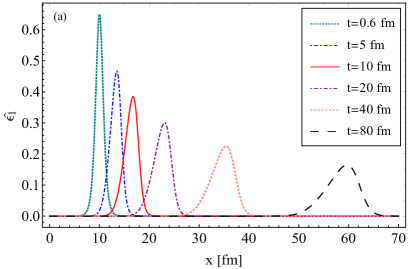
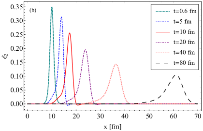
Figure 1: (Color online) (a) $\hat{\epsilon}_{1}$ as a function of $x$ at different time for $A_{1}=0.65$ and $B_{1}=1$ fm. (b) $\hat{\epsilon}_{2}$ as a function of $x$ at different time for $A_{2}=0.35$ and $B_{2}=1$ fm. (c) $\hat{\epsilon}=1+\hat{\epsilon}_{1}+\hat{\epsilon}_{2}$ as a function of $x$ at different time for $A_{1}=0.65,B_{1}=1$ fm, $A_{2}=0.35$ $B_{2}=1$ fm. The background temperature, $T=200$ MeV and $q=1.08$ here.

Firstly, we investigate the effects of non-extensivity only through the EoS, keeping the value of the shear viscosity at the KSS bound Kovtun et al. (2005), $\eta/s=1/4\pi$. The bulk viscosity is taken as $\zeta/s=1/4\pi$ and $\kappa=0$. The value of $T$ and $q$ are taken as $T=200MeV$ and $q=1.08$. Fig. 1(a) and Fig. 1(b) show the time evolution of the spatial shape of the first-order $(\hat{\epsilon_{1}})$ and the second-order $(\hat{\epsilon_{2}})$ perturbations respectively. The initial profile is given by the Eq. (38). In Fig. 1(a), the initial magnitude $(A)$ and width $(B)$ of the first-order perturbation are taken as $A=0.65$, $B=1fm$, whereas in Fig. 1(b), the initial magnitude of the second-order perturbation is taken as $A=0.35$ and width is kept at $B=1fm$. Comparison of results depicted in Fig. 1(a) and Fig. 1(b) indicate that the dissipation of the second-order perturbation is less as compared to first order. This can be understood from the Eq. (30), which indicates that $\hat{\epsilon_{2}}$ gets contributions from $\hat{\epsilon_{1}}$ which contains terms with third-order derivatives in space, known as dispersive term, responsible for preserving the shape of the propagating nonlinear wave. Fig. 1(c) shows the evolution of the energy density up to second order scaled by the background energy density. Though the QGP system produced in heavy-ion collisions has a lifetime of the order of $10-15fm$, we have considered the time evolution up to $80fm$ to have a better understanding of the late time behaviour. It is evident from the results that with time, amplitude decreases and width increases indicating towards the possibility of complete dissipation, unlike the case studied earlier in Ref. Bhattacharyya and Mukherjee (2020). It may be noted that up to $15fm$ the dissipation of the nonlinear wave is not very drastic. The change in amplitude is faster in the beginning than later times. At later time the smaller propagation speed is also noticed. The slowing down of the dissipation can be understood from a comparison of the results displayed in Fig. 1(c), Fig. 2, Fig. 3(a), and Fig. 3(b). In Fig. 1(c) and Fig. 2, the amplitudes of the initial perturbations are taken to be different with the same value of the width, whereas in Fig. 1(c), the amplitude is taken as $A=2$ and in Fig. 2 it is considered to be $A=4$. It is observed that with larger amplitude, the speed of propagation is larger, which is clearly seen in Fig. 2 (the result with $t=80$ fm provides better visibility). This is due to amplitude dependent propagation of nonlinear waves, a well known feature of the nonlinear propagation. The nonlinear waves become slower as the amplitude reduces due to dissipation.

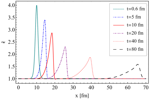
Figure 2: (Color online) $\hat{\epsilon}$ as a function of $x$ at different time for $T=200MeV$, $q=1.08$, $A_{1}=1.65,B_{1}=1,A_{2}=1.35,B_{2}=1$ (parameters are same as in Fig.1(c) but with higher amplitude). We observe that with larger amplitude the speed is larger.

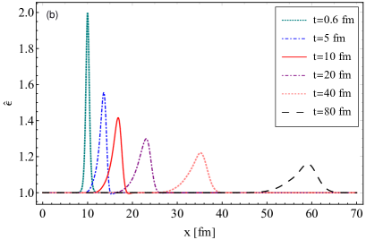
Figure 3: (Color online) (a) $\hat{\epsilon}$ as a function of $x$ at different time for $T=200MeV$, $q=1.08$ $A_{1}=0.65,B_{1}=2,A_{2}=0.35$ and $B_{2}=2$ (parameters are same as in Fig.1 (c)) but with higher width). We observe that the wave propagates faster with lower dissipation as the width increases. (b) Same as Fig. 1(c) with $A_{1}=0.65,B_{1}=0.5,A_{2}=0.35,$ and $B_{2}=0.5$. In this case larger dissipation and smaller speed of propagation is observed.

In Fig. 3(a) and Fig. 3(b), we compare the results for the widths taken as $B=2fm$ and $B=0.5fm$ respectively with the same value of the amplitude ($A=2$). It is observed that the increase in width of the initial perturbation causes less dissipation with the progression of time for the same background fluid conditions. The propagation speed is found to be greater for perturbation with larger width. This is because, the perturbation with larger width dissipates less, and thus due to amplitude dependent speed of propagation, it propagates faster in space. Comparison of results presented in Fig. 2 and Fig. 3 indicates that the increase in amplitude or in width reduces the damping but increases the speed of the peak position.

Now we move to discuss the role of the background of the fluid, inscribed through $q$ and $T$, on the perturbations. We take the same values of $A_{1}$, $A_{2}$, $B_{1}$ and $B_{2}$ as in Fig.1(c) to study the fate of the perturbations after $t=10$ fm for three different values of the background temperatures and fixed value of $q=1.08$. The result is displayed in Fig. 4. We find that the dissipation decreases with increase in the background temperature but the perturbation in the front becomes steep. However, for ideal background, the magnitude as well as the tilting remain unchanged with the variation of the background temperature. In the present work we consider the background energy density as a function of temperature in contrast to previous work Bhattacharyya and Mukherjee (2020) on ideal hydrodynamic background at fixed background energy density with varying temperature.

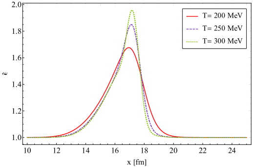
Figure 4: (Color online) $\hat{\epsilon}$ as a function of $x$ at time $t=10$ fm for different $T$. Other parameters are $q=1.08$, $A_{1}=0.65,B_{1}=1,A_{2}=0.35,B_{2}=1$. We observe smaller dissipation at larger temperature.

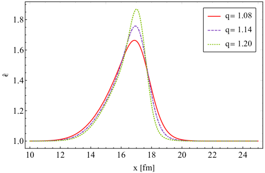
Figure 5: (Color online) $\hat{\epsilon}$ as a function of $x$ at time $t=10$ fm and $T=200$ MeV for different values of $q$. The amplitudes and the widths of the perturbations are defined by Eq. (38) with $A_{1}=0.65,B_{1}=1,A_{2}=0.35,B_{2}=1$. Smaller dissipation and tilting along $x$ axis have been seen for larger $q$.

Figure 6: (Color online) $\hat{\epsilon}$ as a function of $x$ for different time for ideal fluid ($\eta=\zeta=0$). We take $T=200$ MeV, $q=1.08$, $A_{1}=0.65,B_{1}=1,A_{2}=0.35$ and $B_{2}=1$. We observe that the waves tend to loose their localization with time.

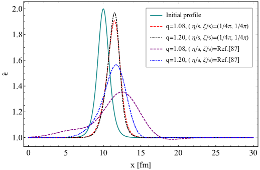
Figure 7: (Color online) The variation of $\hat{\epsilon}$ with spatial coordinate ($x$) at $t=2$ fm for different values of $q$ and viscous coefficients have been shown here. The temperature of the fluid, $T=200$ MeV. The values of $A_{1},A_{2}$, $B_{1}$, and $B_{2}$ are same as Fig.1(c).

Fig. 5 shows the fate of the same initial perturbation as that of displayed in Fig. 1(c) after a time of $10$ fm for three different values of $q$ for $T=200$ MeV. In the presence of dissipation the $q$ plays an interesting role. Namely for higher values of $q$ the dissipation is lower and the stiffness is more. In the absence of dissipation (ideal background) we also find more stiffness for higher $q$ Bhattacharyya and Mukherjee (2020). Indicating that the effects of dissipation can be reduced by increasing $q$, or in other words systems with higher $q$ imitate lower dissipation. It is also to be noted from the results shown in Fig. 5 that the propagation speed of the peak increases with $q$ if the $q$ dependence is considered only through EoS. The results of ideal $q$-hydrodynamics can be obtained from our results by setting the values of the transport coefficients to zero. In Fig. 6 the results for vanishingly small transport coefficients have been shown. In such cases we find that the waves loose their localization (breaking waves) and the shape preserving nature no longer survives.

So far we have discussed the effects of non-extensivity on the propagation of nonlinear waves only through the EoS. Since the EoS and transport coefficients control the bulk evolution of a system, therefore, for a thorough treatment of the propagation of nonlinear waves in a non-extensive background ($q$-background), one should consider the effects of non-extensivity, not only through the EoS ($q$-EoS) but also on the transport coefficients ($q$-viscosities) which are estimated for $q$-background (see Biro and Molnar (2012); Kadam and Mishra (2015) for details). The results with the $q$-viscosities ($q$-dependence of viscous coefficients) along with the $q$-EoS (as discussed in section III) are presented in Fig. 7 (purple and blue dashed lines) for the initial profile shown by green line. The results obtained with the effects of $q$-EoS only is compared (black and red dashed lines). It is found that the dissipation of nonlinear waves is more when non-extensivity is introduced via the $q$-EoS and the $q$-viscosities together. Interestingly, here, the propagation speed of the peak of the perturbations decrease with the increasing value of $q$ when the effects of $q$-viscosity is introduced. Along with the reduction of the dissipation the higher values of $q$ also reduces the speed of the propagation. This means that the introduction of non-extensivity favours the non-dissipative (or anti-dissipative) slowing down of nonlinear perturbations. Considering the fact that for an extensive background, the slowing down is caused by the dissipative effects Sarwar et al. (2021), the results displayed in Fig. 7 reveal that the propagation of non-linear wave can be useful to distinguish between the extensive and the non-extensive background. We also find that the dissipation is more for smaller $q$-values (compare with Fig. 5). With the q-viscosities along with q-EoS, the relative dissipation with $q$ is more than that of the q-EoS only. This is in contrast to the expectation from the notion that the non-extensive distribution is treated as a non-equilibrium deviation from the extensive one. In such a scenario the dissipative correction is interpreted as a result of $q\neq 1$. These findings are opposite to the normal expectations. Rather, it indicates that $q$-equilibrium should not always be interpreted as a dissipative non-equilibrium form of extensive statistics.

In a system with $q$-background, the higher values of $q$ is accompanied by less dissipation in the system. This can be understood from the fact that the enhanced correlation in a system can be represented by higher $q$-values Lima and Deppman (2020); Abe (1999). The correlations enhance the fluctuations, which can also be represented by a value of $q\neq 1$ Wilk and Wlodarczyk (2000). The correlations opposes the entropy generation in a system and hence dissipation. Therefore, a higher value of $q$ parameter representing a higher degree of correlation which is expected to results in less dissipation, this is manifested in the variation of viscosity to entropy ratio ($\eta/s$) with $q$ Biro and Molnar (2012). The $\eta/s$ decreases with increasing $q$ due to greater rate of change of non-extensive entropy with $q$ than of the bulk and shear viscosities, thereby reducing the dissipation.

The second and higher order space derivatives in the evolution equations contain the effects of dissipation. Without the presence of the viscous terms, the $q$ alone (through $q$-EoS only) can not produce such dissipative nature, i.e, $q$ can only have a role in dissipation in the presence of explicit dissipative terms. That is why, without considering the $q$-viscosities (or any dissipative effects arising from $d$-hydrodynamics), the authors in Bhattacharyya and Mukherjee (2020) do not find any dissipation with $q$-EoS alone. Also they have considered only the first order of energy perturbation and found that the equation to be of the breaking-wave type, causing a tilting (ultimately breaking) of nonlinear waves without any dissipation. Whereas, in this work we have obtained KdV type equation by considering perturbations up to second-order with the inclusion of all the relevant transport coefficients and found to produce prominent dissipative effects without much tilting.

In such a scenario, one may be tempted to think that, perhaps, less dissipation is the unique signature of presence of finite $q$ (increasing $q$-values). However, it may be noted that the less dissipation may be accounted through the smaller values of the transport coefficients also. So there may be an ambiguity behind the observed smaller dissipation in a system, whether it is a non-extensive system with larger values of $q$ or it is an extensive system with lower viscosity. Such ambiguity can be removed through other effects which can distinguish these two separate situations. The role of higher values of $q$ as the cause of less dissipation can be mimicked by reducing the values of the transport coefficients, but it may possess other distinct effects which will help in removing the ambiguity. In the case of nonlinear wave propagation, the nature of the nonlinear wave will provide the relevant distinct feature. With less dissipation in extensive background (i.e without $q$-background) the nonlinear wave will not preserve the solitonic nature due to breaking of the wave (see Fig. 6), whereas the $q$ makes the dissipation less with preserving the solitonic nature (see Fig. 7). Therefore, the causes for less dissipation with Tsallis background can be distinguished with the propagation of a nonlinear wave. This may pave the way for investigation to ascertain whether the viscosity of the QGP is really low or it has $q$-thermalized local equilibrium with not so low transport coefficients. Since $p+p$ collision admits $q$-distributed particle spectra, therefore, one would argue for consideration of $q$-thermalized local equilibrium. In that case it is very important to remove the ambiguity about viscosities of QGP estimated by fitting the experimental results. Another important point to be noted is that, when the ideal $q$-hydrodynamics is interpreted as equivalent to $d$-hydrodynamics, one should not take $q$ as a cause of dissipation in general sense. This is so because, $q$ does not necessarily represents dissipation, especially when the background is in $q$ equilibrium.

V Summary and conclusion

In summary, we have derived the equations for the propagation of nonlinear waves in a dissipative fluid involving shear viscosity, bulk viscosity and thermal conductivity. The effect of the $q-$statistics is incorporated by taking into account the $q-$EoS and $q$-viscosities. We find that the equation for the second order perturbation is similar to the KdV equation resulting in the solitonic nature of nonlinear waves. It is observed that the dissipation of the wave is more in first order than the second order. For larger amplitude of the perturbations, we find that the speed of the propagation is larger, whereas for broader perturbations, the dissipation is comparatively less and propagation is faster. As far as the background temperature of the medium is concerned, dissipation is less for higher temperature. The effect of $q$ is evident from the results shown in Fig.5, where we see more dissipation of nonlinear waves for smaller values of $q$. This is in line with the interpretation of $q$ as representative of correlations as well as fluctuations in a system. The larger values of $q$ may imitate the situation with smaller values of the transport coefficients. This is reflected through the maintenance of solitonic nature of the nonlinear waves. Moreover, it is found that the non-extensivity favours the non-dissipative slowing down of nonlinear perturbations. This is in contrast to the extensive background where the slowing down comes with the dissipation Sarwar et al. (2021). This may be a useful criterion for making distinction between the extensive and non-extensive background. So the nature of propagation of a nonlinear wave can be potentially used to distinguish a non-extensive medium from an extensive one, which could be especially helpful in situations where momentum distribution of particles can not distinguish the nature of underlying statistics (Gibbs-Boltzmann or Tsallis). This indistinguishability may occur when there is an uncertainty on whether the equilibration is complete or not and when there are other sources of power law distributions such as the radiation from particles with high momentum or jets moving through the QGP, instead of the presence of correlations that causes non-extensivity of the medium.

VI Acknowledgement

MH, MR would like to thank Department of Higher Education, Govt. of West Bengal, India. TB acknowledges partial support from the joint project between the JINR and IFIN-HH. The work of AB is supported by Alexander von Humboldt (AvH) foundation and Federal Ministry of Education and Research (Germany) through Research Group Linkage programme.

Appendix A

In this appendix we provide the expressions for the relaxation and coupling coefficients Israel and Stewart (1979) required to solve the Israel-Stewart hydrodynamical equations.

$$\alpha_{0} = (D_{41}D_{20}-D_{31}D_{30})\Lambda\phi\Omega J_{21}J_{31}~{},$$

$$\alpha_{1} = (J_{41}J_{42}-J_{31}J_{52})\Lambda\phi J_{21}J_{31}~{},$$

$$\beta_{0} = \frac{3\beta}{\phi^{2}\Omega^{2}}[5J_{52}-\frac{3}{D_{20}}\{J_{31}(J_{31}J_{30}-J_{41}J_{20})+J_{41}(J_{41}J_{10}-J_{31}J_{20})\}]~{},$$

$$\beta_{1} = \frac{D_{41}}{\Lambda^{2}nmJ_{21}J_{31}}~{},$$

$$\beta_{2} = \frac{\beta J_{52}}{2\phi^{2}}~{},$$ (39)

where,

$$D_{rs} = J_{r+1,s}J_{r-1,s}-(J_{rs})^{2},\,\,\,\,\phi=T(\epsilon+P),\,\,\,\,\psi=\frac{\epsilon+p}{n_{i}m_{i}},$$

$$\Lambda = 1+5(\frac{\phi}{nm})-\psi^{2},\,\,\,\,\Omega=3\Big{(}\frac{\partial ln\phi}{\partial lnn}\Big{)}-5~{},$$ (40)

where $r$, $s$ are integers, $m_{i}$ and $n_{i}$ are respectively the mass and density of $i$-th type particle. The quantities, $\phi,\psi$ and $\Lambda$ are calculated by using their relations with $\epsilon$, $p$ and $n_{i}$. We take the current quark mass of up and down flavors as 10 MeV. $J_{rs}$ is defined as,

$$J_{rs}=\frac{A_{0}}{(2s+1)!!}\int_{0}^{\infty}N\Delta Sinh^{2(s+1)}\mathcal{R}Cosh^{r-2s}\mathcal{R}d\mathcal{R}~{},$$ (41)

and

$$N=\frac{1}{exp_{q}(\beta Cosh\mathcal{R}-\alpha)-\epsilon}~{},$$ (42)

where, $q$-deformed exponential is defined as,

$$exp_{q}(x)=\big{[}1+(1-q)x\big{]}^{1/(1-q)}~{},$$ (43)

and

$$\Delta=1+\epsilon N,\,\,\,\,A_{0}=4\pi m_{i}^{3}~{}.$$ (44)

These coupling and relaxation coefficients in Landau frame are connected to the coupling and relaxation coefficients in the Eckart frame by the following relation Israel and Stewart (1979)

$$\tilde{\alpha_{0}}-\alpha_{0}=\tilde{\alpha_{1}}-\alpha_{1}=-(\tilde{\beta_{1}}-\beta_{0})=-[(\epsilon+p)]^{-1}$$ (45)

Appendix B

The coefficients $\mathcal{S}_{i}$’s for $i=1$ to $5$ appearing in Eq. (30) are given in this appendix.

$$\mathcal{S}_{1} = \frac{1}{\epsilon_{0}+p_{0}}\Big{[}c_{s}\{\epsilon_{0}\left(1-\hat{\epsilon}_{1}\left(c_{s}^{2}-1\right)\right)+p_{0}\}\Big{]};$$

$$\mathcal{S}_{2} = \frac{1}{\epsilon_{0}+p_{0}}\Big{[}\epsilon_{0}c_{s}\{c_{s}^{2}-1\}\{\epsilon_{0}\left(\left(2c_{s}^{2}+1\right)\hat{\epsilon}_{1}{}^{2}-\hat{\epsilon}_{2}\right)-p_{0}\hat{\epsilon}_{2}\}\Big{]};$$

$$\mathcal{S}_{3} = \frac{1}{12(\epsilon_{0}+p_{0})^{2}}\Big{[}\epsilon_{0}\hat{\epsilon}_{1}\{3c_{s}^{2}(7\zeta+8\eta)+3\zeta+4\eta\}\Big{]};$$

$$\mathcal{S}_{4} = -\frac{1}{72c_{s}c_{V}(\epsilon_{0}+p_{0})^{2}}\Big{[}4c_{V}c_{s}^{2}\{3\kappa T\epsilon_{0}(3\alpha_{0}\zeta+4\alpha_{1}\eta)+3\kappa T(3\zeta+4\eta)+3\kappa Tp_{0}(3\alpha_{0}\zeta+4\alpha_{1}\eta)$$

$$+(\epsilon_{0}+p_{0})(9\beta_{0}\zeta^{2}+16\beta_{2}\eta^{2})\}-c_{V}(3\zeta+4\eta)^{2}+12\kappa\{\epsilon_{0}+p_{0}\}\{\epsilon_{0}(3\alpha_{0}\zeta+4\alpha_{1}\eta)+3\zeta+4\eta$$

$$+p_{0}(3\alpha_{0}\zeta+4\alpha_{1}\eta)\}\Big{]};$$

$${\text{a}nd}$$ (46)

$$\mathcal{S}_{5} = -\frac{3\zeta+4\eta}{6\left(p_{0}+\epsilon_{0}\right)}~{}.$$ (47)

Appendix C

In this appendix the expressions for $\epsilon_{i,\ell}$ and $P_{i,\ell}$ ($i=F,B$; $\ell=1,2$) are provided as follows. ($i=F,B$; $\ell=1,2$) are given by Bhattacharyya and Mukherjee (2020),

$$\epsilon_{B,1} = \frac{g}{2\pi^{2}(q-1)^{3}q}\left[3\psi^{(0)}\left(\frac{3}{q}-2\right)+\psi^{(0)}\left(\frac{1}{q}\right)\right.\left.-3\psi^{(0)}\left(\frac{2}{q}-1\right)-\psi^{(0)}\left(\frac{4}{q}-3\right)\right],$$ (48)

$$\epsilon_{F,1} = \frac{g}{2\pi^{2}(q-1)^{3}q}\left[3\Phi\left(-1,1,\frac{2}{q}-1\right)-3\Phi\left(-1,1,\frac{3}{q}-2\right)+\Phi\left(-1,1,\frac{4}{q}-3\right)\right.$$ (49)

$$\left.-\Phi\left(-1,1,\frac{1}{q}\right)\right],$$

$$\epsilon_{F,2} = -\frac{g}{4\pi^{2}(q-1)q}\left[\Phi\left(-1,1,\frac{2}{q}-1\right)\right.\left.-\Phi\left(-1,1,\frac{1}{q}\right)\right],$$ (50)

$$P_{B,1} = \frac{\epsilon_{B,1}}{3},~{}P_{F,1}=\frac{\epsilon_{F,1}}{3},~{}P_{F,2}=\epsilon_{F,2}~{},$$ (51)

where $\psi^{(0)}$ is the digamma function, and $\Phi$ is another special function known as Lerch’s transcendent W. Magnus (1981).

References

- Kirtskhalia (2016) V. Kirtskhalia, Journal of Fluids 2016, 1 (2016), URL https://app.dimensions.ai/details/publication/pub.1002429324andhttp://downloads.hindawi.com/archive/2016/4519201.pdf.
- Lick (1990) W. Lick, Wave Propagation (Springer US, Boston, MA, 1990), pp. 815–877, ISBN 978-1-4684-1423-3, URL https://doi.org/10.1007/978-1-4684-1423-3_15.
- Busza et al. (2018) W. Busza, K. Rajagopal, and W. van der Schee, Ann. Rev. Nucl. Part. Sci. 68, 339 (2018), eprint 1802.04801.
- Shuryak (2009) E. Shuryak, Phys. Rev. C 80, 054908 (2009), [Erratum: Phys.Rev.C 80, 069902 (2009)], eprint 0903.3734.
- Betz (2009) B. Betz, Ph.d. thesis (2009), eprint 0910.4114.
- Staig and Shuryak (2011a) P. Staig and E. Shuryak, Phys. Rev. C 84, 034908 (2011a), eprint 1008.3139.
- Staig and Shuryak (2011b) P. Staig and E. Shuryak, Phys. Rev. C 84, 044912 (2011b), eprint 1105.0676.
- Sarwar and Alam (2018) G. Sarwar and J.-e. Alam, Int. J. Mod. Phys. A 33, 1850040 (2018), eprint 1503.06019.
- Rafiei and Javidan (2016) A. Rafiei and K. Javidan, Phys. Rev. C 94, 034904 (2016).
- Hasanujjaman et al. (2020) M. Hasanujjaman, M. Rahaman, A. Bhattacharyya, and J.-e. Alam, Phys. Rev. C 102, 034910 (2020), eprint 2003.07575.
- Hasanujjaman et al. (2021) M. Hasanujjaman, G. Sarwar, M. Rahaman, A. Bhattacharyya, and J.-e. Alam, Eur. Phys. J. A 57, 283 (2021), eprint 2008.03931.
- Minami and Kunihiro (2010) Y. Minami and T. Kunihiro, Prog. Theor. Phys. 122, 881 (2010), eprint 0904.2270.
- Rahaman and Alam (2018) M. Rahaman and J.-e. Alam, Phys. Rev. C 97, 054906 (2018), eprint 1712.09175.
- Raha et al. (1985) S. Raha, K. Wehrberger, and R. M. Weiner, Nucl. Phys. A 433, 427 (1985).
- Fowler et al. (1982) G. N. Fowler, S. Raha, N. Stelte, and R. M. Weiner, Phys. Lett. B 115, 286 (1982).
- Raha and Weiner (1983) S. Raha and R. M. Weiner, Phys. Rev. Lett. 50, 407 (1983).
- Hefter et al. (1985) E. F. Hefter, S. Raha, and R. M. Weiner, Phys. Rev. C 32, 2201 (1985).
- Fogaça et al. (2010) D. A. Fogaça, L. G. Ferreira Filho, and F. S. Navarra, Phys. Rev. C 81, 055211 (2010), eprint 0908.4215.
- Fogaça et al. (2014) D. A. Fogaça, H. Marrochio, F. S. Navarra, and J. Noronha, Nucl. Phys. A 934, 18 (2014), eprint 1402.5548.
- Sarwar et al. (2021) G. Sarwar, M. Hasanujjaman, M. Rahaman, A. Bhattacharyya, and J.-e. Alam, Phys. Lett. B 820, 136583 (2021), eprint 2012.12668.
- Tsallis (1988) C. Tsallis, J. Statist. Phys. 52, 479 (1988).
- Constantino (2009) T. Constantino, Introduction to Nonextensive Statistical Mechanics (Springer-Verlag New York, 2009).
- Khachatryan et al. (2010) V. Khachatryan et al. (CMS), Phys. Rev. Lett. 105, 022002 (2010), eprint 1005.3299.
- Acharya et al. (2018) S. Acharya et al. (ALICE), Phys. Rev. C 97, 024615 (2018), eprint 1709.08522.
- Biro et al. (2009) T. S. Biro, G. Purcsel, and K. Urmossy, Eur. Phys. J. A 40, 325 (2009), eprint 0812.2104.
- Cleymans et al. (2013) J. Cleymans, G. I. Lykasov, A. S. Parvan, A. S. Sorin, O. V. Teryaev, and D. Worku, Phys. Lett. B 723, 351 (2013), eprint 1302.1970.
- Marques et al. (2015) L. Marques, J. Cleymans, and A. Deppman, Phys. Rev. D 91, 054025 (2015), eprint 1501.00953.
- Bhattacharyya et al. (2016a) T. Bhattacharyya, J. Cleymans, A. Khuntia, P. Pareek, and R. Sahoo, Eur. Phys. J. A 52, 30 (2016a), eprint 1507.08434.
- Tripathy et al. (2016) S. Tripathy, T. Bhattacharyya, P. Garg, P. Kumar, R. Sahoo, and J. Cleymans, Eur. Phys. J. A 52, 289 (2016), eprint 1606.06898.
- Grigoryan (2017) S. Grigoryan, Phys. Rev. D 95, 056021 (2017), eprint 1702.04110.
- Bhattacharyya et al. (2018) T. Bhattacharyya, J. Cleymans, L. Marques, S. Mogliacci, and M. W. Paradza, J. Phys. G 45, 055001 (2018), eprint 1709.07376.
- Azmi et al. (2020) M. D. Azmi, T. Bhattacharyya, J. Cleymans, and M. Paradza, J. Phys. G 47, 045001 (2020), eprint 1911.04878.
- Wong et al. (2015) C.-Y. Wong, G. Wilk, L. J. L. Cirto, and C. Tsallis, Phys. Rev. D 91, 114027 (2015), eprint 1505.02022.
- Azmi and Cleymans (2015) M. D. Azmi and J. Cleymans, Eur. Phys. J. C 75, 430 (2015), eprint 1501.07127.
- Cleymans and Worku (2012) J. Cleymans and D. Worku, Eur. Phys. J. A 48, 160 (2012), eprint 1203.4343.
- Zheng and Zhu (2016) H. Zheng and L. Zhu, Adv. High Energy Phys. 2016, 9632126 (2016), eprint 1512.03555.
- Wilk and Wlodarczyk (2000) G. Wilk and Z. Wlodarczyk, Phys. Rev. Lett. 84, 2770 (2000), eprint hep-ph/9908459.
- Tsallis and Bukman (1996) C. Tsallis and D. J. Bukman, Physical Review E 54, R2197 (1996), ISSN 1095-3787, URL http://dx.doi.org/10.1103/PhysRevE.54.R2197.
- Boghosian et al. (2003) B. M. Boghosian, P. J. Love, P. V. Coveney, I. V. Karlin, S. Succi, and J. Yepez, Phys. Rev. E 68, 025103 (2003), URL https://link.aps.org/doi/10.1103/PhysRevE.68.025103.
- Douglas et al. (2006) P. Douglas, S. Bergamini, and F. Renzoni, Phys. Rev. Lett. 96, 110601 (2006).
- Deppman et al. (2020a) A. Deppman, E. Megías, and D. P. Menezes, Phys. Scripta 95, 094006 (2020a), eprint 2002.12667.
- Deppman et al. (2020b) A. Deppman, E. Megías, and D. P. Menezes, Phys. Rev. D 101, 034019 (2020b), eprint 1908.08799.
- Deppman et al. (2020c) A. Deppman, E. Megías, and D. P. Menezes, MDPI Physics 2, 455 (2020c), eprint 2008.03236.
- Lima and Deppman (2020) J. A. S. Lima and A. Deppman, Phys. Rev. E 101, 040102 (2020), eprint 2004.12534.
- Rozynek and Wilk (2016) J. Rozynek and G. Wilk, Eur. Phys. J. A 52, 294 (2016), eprint 1606.09033.
- Rożynek and Wilk (2019) J. Rożynek and G. Wilk, Symmetry 11, 401 (2019), eprint 1810.07008.
- Bhattacharyya et al. (2016b) T. Bhattacharyya, J. Cleymans, and S. Mogliacci, Phys. Rev. D 94, 094026 (2016b), eprint 1608.08965.
- Navarra et al. (2003) F. S. Navarra, O. V. Utyuzh, G. Wilk, and Z. Wlodarczyk, Phys. Rev. D 67, 114002 (2003), eprint hep-ph/0301258.
- Navarra et al. (2004) F. S. Navarra, O. V. Utyuzh, G. Wilk, and Z. Wlodarczyk, Physica A 344, 568 (2004), eprint hep-ph/0312136.
- Biyajima et al. (2005) M. Biyajima, M. Kaneyama, T. Mizoguchi, and G. Wilk, Eur. Phys. J. C 40, 243 (2005), eprint hep-ph/0403063.
- Biyajima et al. (2006) M. Biyajima, T. Mizoguchi, N. Nakajima, N. Suzuki, and G. Wilk, Eur. Phys. J. C 48, 597 (2006), eprint hep-ph/0602120.
- Wilk and Wlodarczyk (2002) G. Wilk and Z. Wlodarczyk, Chaos Solitons Fractals 13, 581 (2002), eprint hep-ph/0004250.
- Wilk and Wlodarczyk (2009) G. Wilk and Z. Wlodarczyk, Phys. Rev. C 79, 054903 (2009), eprint 0902.3922.
- Biro and Jakovac (2005) T. S. Biro and A. Jakovac, Phys. Rev. Lett. 94, 132302 (2005), eprint hep-ph/0405202.
- Deb et al. (2021) S. Deb, G. Sarwar, R. Sahoo, and J.-e. Alam, Eur. Phys. J. A 57, 195 (2021), eprint 1909.02837.
- Das et al. (2020a) A. Das, W. Florkowski, R. Ryblewski, and R. Singh (2020a), eprint 2012.05662.
- Das et al. (2021a) A. Das, W. Florkowski, R. Ryblewski, and R. Singh, Phys. Rev. D 103, L091502 (2021a), eprint 2103.01013.
- Das et al. (2021b) A. Das, W. Florkowski, R. Ryblewski, and R. Singh (2021b), eprint 2105.02125.
- Osada and Wilk (2008) T. Osada and G. Wilk, Phys. Rev. C 77, 044903 (2008), [Erratum: Phys.Rev.C 78, 069903 (2008)], eprint 0710.1905.
- Bhattacharyya and Mukherjee (2020) T. Bhattacharyya and A. Mukherjee, Eur. Phys. J. C 80, 656 (2020), eprint 2003.10692.
- Biro and Molnar (2012) T. S. Biro and E. Molnar, Phys. Rev. C 85, 024905 (2012), eprint 1109.2482.
- Eckart (1940) C. Eckart, Phys. Rev. 58, 919 (1940).
- Landau and Lifshitz (1987) L. Landau and E. Lifshitz (Pergamon, 1987), second edition ed., ISBN 978-0-08-033933-7.
- Bemfica et al. (2018) F. S. Bemfica, M. M. Disconzi, and J. Noronha, Phys. Rev. D 98, 104064 (2018), eprint 1708.06255.
- Bemfica et al. (2019) F. S. Bemfica, M. M. Disconzi, and J. Noronha, Phys. Rev. D 100, 104020 (2019), eprint 1907.12695.
- Bemfica et al. (2020) F. S. Bemfica, M. M. Disconzi, and J. Noronha (2020), eprint 2009.11388.
- Kovtun (2019) P. Kovtun, JHEP 10, 034 (2019), eprint 1907.08191.
- Das et al. (2020b) A. Das, W. Florkowski, J. Noronha, and R. Ryblewski, Phys. Lett. B 806, 135525 (2020b), eprint 2001.07983.
- Das et al. (2020c) A. Das, W. Florkowski, and R. Ryblewski, Phys. Rev. D 102, 031501 (2020c), eprint 2006.00536.
- Israel and Stewart (1979) W. Israel and J. M. Stewart, Annals Phys. 118, 341 (1979).
- Hiscock and Lindblom (1983) W. A. Hiscock and L. Lindblom, Annals Phys. 151, 466 (1983).
- Koide et al. (2007) T. Koide, G. S. Denicol, P. Mota, and T. Kodama, Phys. Rev. C 75, 034909 (2007), eprint hep-ph/0609117.
- Romatschke (2010) P. Romatschke, Int. J. Mod. Phys. E 19, 1 (2010), eprint 0902.3663.
- Van and Biro (2008) P. Van and T. S. Biro, Eur. Phys. J. ST 155, 201 (2008), eprint 0704.2039.
- Tsumura and Kunihiro (2010) K. Tsumura and T. Kunihiro, Phys. Lett. B 690, 255 (2010), eprint 0906.0079.
- Muronga (2004) A. Muronga, Phys. Rev. C 69, 034903 (2004), eprint nucl-th/0309055.
- Muronga (2002) A. Muronga, Phys. Rev. Lett. 88, 062302 (2002), [Erratum: Phys.Rev.Lett. 89, 159901 (2002)], eprint nucl-th/0104064.
- Washimi and Taniuti (1966) H. Washimi and T. Taniuti, Phys. Rev. Lett. 17, 996 (1966), URL https://link.aps.org/doi/10.1103/PhysRevLett.17.996.
- Davidson (1972) R. C. Davidson, Methods in Nonlinear Plasma Theory, vol. 37 (Academic Press, New York, 1972).
- Leblond (2008) H. Leblond, Journal of Physics B 41, 043001 (2008), URL https://doi.org/10.1088/0953-4075/41/4/043001.
- Kraenkel et al. (1995) R. A. Kraenkel, M. A. Manna, J. C. Montero, and J. G. Pereira, arXiv e-prints patt-sol/9509003 (1995), eprint patt-sol/9509003.
- Rahaman et al. (2021) M. Rahaman, T. Bhattacharyya, and J.-e. Alam, Int. J. Mod. Phys. A 36, 2150154 (2021), eprint 1906.02893.
- Chodos et al. (1974) A. Chodos, R. L. Jaffe, K. Johnson, C. B. Thorn, and V. F. Weisskopf, Phys. Rev. D 9, 3471 (1974), URL https://link.aps.org/doi/10.1103/PhysRevD.9.3471.
- Lavagno et al. (2010) A. Lavagno, D. Pigato, and P. Quarati, J. Phys. G 37, 115102 (2010), eprint 1005.4643.
- Cardoso et al. (2017) P. H. G. Cardoso, T. Nunes da Silva, A. Deppman, and D. P. Menezes, Eur. Phys. J. A 53, 191 (2017), eprint 1706.02183.
- Kovtun et al. (2005) P. Kovtun, D. T. Son, and A. O. Starinets, Phys. Rev. Lett. 94, 111601 (2005), eprint hep-th/0405231.
- Kadam and Mishra (2015) G. P. Kadam and H. Mishra, Phys. Rev. C 92, 035203 (2015), eprint 1506.04613.
- Abe (1999) S. Abe, Physica A 269, 403 (1999), ISSN 0378-4371, URL https://www.sciencedirect.com/science/article/pii/S0378437199000643.
- W. Magnus (1981) F. T. W. Magnus, F. Oberhettinger, Higher Transcendental Functions, vol. 1 (Krieger Publishing Company, 1981).