Rank Overspecified Robust Matrix Recovery: Subgradient Method and Exact Recovery

Abstract

We study the robust recovery of a low-rank matrix from sparsely and grossly corrupted Gaussian measurements, with no prior knowledge on the intrinsic rank. We consider the robust matrix factorization approach. We employ a robust $\ell_{1}$ loss function and deal with the challenge of the unknown rank by using an overspecified factored representation of the matrix variable. We then solve the associated nonconvex nonsmooth problem using a subgradient method with diminishing stepsizes. We show that under a regularity condition on the sensing matrices and corruption, which we call restricted direction preserving property (RDPP), even with rank overspecified, the subgradient method converges to the exact low-rank solution at a sublinear rate. Moreover, our result is more general in the sense that it automatically speeds up to a linear rate once the factor rank matches the unknown rank. On the other hand, we show that the RDPP condition holds under generic settings, such as Gaussian measurements under independent or adversarial sparse corruptions, where the result could be of independent interest. Both the exact recovery and the convergence rate of the proposed subgradient method are numerically verified in the overspecified regime. Moreover, our experiment further shows that our particular design of diminishing stepsize effectively prevents overfitting for robust recovery under overparameterized models, such as robust matrix sensing and learning robust deep image prior. This regularization effect is worth further investigation.

1 Introduction

Robust low rank matrix recovery problems are ubiquitous in computer vision [1], signal processing [2], quantum state tomography [3], etc. In the vanilla setting, the task is to recover a rank $r$ positive semidefinite (PSD) matrix $X_{\natural}\in\mathbb{R}^{d\times d}$ ($r\ll d$) from a few corrupted linear measurements $\{(y_{i},A_{i})\}_{i=1}^{n}$ of the form

$$y_{i}=\left\langle A_{i},X_{\natural}\right\rangle+s_{i},\quad i=1,\dots,m,$$ (1.1)

where $\left\{s_{i}\right\}_{i=1}^{m}$ are the corruptions. This model can be written succinctly as $y=\mathcal{A}(X_{\natural})+s$, where $\mathcal{A}:\mathbb{R}^{d\times d}\to\mathbb{R}^{m}$ is the measurement operator. Recently, tremendous progress has been made on this problem, leveraging advances on convex relaxation [1, 2], nonconvex optimization [4, 5, 6, 7], and high dimension probability [8, 9, 10, 11]. However, several practical challenges remain:

• Nonconvex and nonsmooth optimization for sparse corruptions. For computational efficiency, we often exploit the low-rank structure via the factorization $X=FF^{\top}$ with $F\in\mathbb{R}^{d\times r}$, and solve the problem with respect to $F$ via nonconvex optimization. This problem is challenging since the corruption can be arbitrary. Fortunately, the corruptions $s_{i}$ are sparse [1]. This motivates us to consider the $\ell_{1}$ loss function and lead to a nonsmooth nonconvex problem.

• Unknown rank and overspecification. Another major challenge in practice is that the exact true rank $r$ is usually unknown apriori. To deal with this issue, researchers often solve the problem in rank overspecified regime, using a factor variable $F\in\mathbb{R}^{d\times k}$ with a larger inner dimension $k>r$. Most existing analysis relies on the $k$-th eigenvalue of $X_{\natural}$ being nonzero and is inapplicable in this setting. Recent work studied the problem either in some special case (e.g., rank one) [13] or under unrealistic communitability conditions [14].

Our approach and contributions.

To deal with these challenges, we consider the following nonconvex and nonsmooth formulation with overspecified rank $k\geq r$,

$$\min_{F\colon F\in\mathbb{R}^{d\times k}}f(F):=\frac{1}{2m}\sum_{i=1}^{m}\left|\left\langle A_{i},FF^{\top}\right\rangle-y_{i}\right|=\frac{1}{2m}\left\|\mathcal{A}(FF^{\top})-y\right\|_{1},$$ (1.2)

and solve the problem using a subgradient method with adaptive stepsize. We summarize our contributions as follows.

• Exact recovery with rank overspecification. In 3.2, we show that under Gaussian measurements and sparse corruptions, with $m=\tilde{\mathcal{O}}(dk^{3})$ samples, even with overspecified rank $k>r$, our subgradient method with spectral initialization converges to the ground truth $X_{\natural}$ exactly. When $k>r$, the convergence rate is $\mathcal{O}(\frac{1}{t})$ in the operator norm error $\left\|F_{t}F_{t}^{\top}-X_{\natural}\right\|$. When $k=r$, the convergence rate boosts to a linear (geometric) rate.

• Convergence under a regularity condition. Our convergence result is established under a regularity condition termed restricted direction preserving property (RDPP); see Definition 2.1. RDPP ensures that the direction of the finite-sample subgradient stays close to its population version along the algorithm’s iteration path. The key to our proof is to use this property to leverage a recent result on rank overspecification under smooth formulations [15]. Moreover, we show that RDPP holds with high probability under arbitrary sparse corruptions and Gaussian measurement matrices.

• Adaptive stepsize and implicit regularization. As shown in [14, 13], for overparametrized robust matrix recovery problems, subgradient methods with constant stepsizes suffer from overfitting, even when initialized near the origin. In contrast, numerical experiments demonstrate that our theory-inspired diminishing stepsize rule has an implicit regularization effect that prevents overfitting. Our stepsize rule is easy to implement and almost tuning-free, and performs better than other non-adaptive stepsize rules (e.g., sublinear or geometric decaying stepsizes). We demonstrate similar good performance of our method (with a fixed decaying stepsize) in image recovery with a robust deep image prior (DIP) [16].

Related work.

The nonconvex, factorized formulation (1.2) is computationally more efficient than convex relaxation approaches [17, 1, 18, 19], as it involves a smaller size optimization variable and only requires one partial singular value decomposition (SVD) in the initialization phase. In the corruption-free ($s_{i}\equiv 0$) and exact rank ($k=r$) setting, provably efficient methods have been studied for the smooth, least squares version of (1.2) [20, 21, 22, 23]; in this case, the loss function has no spurious local minimum and is locally strongly convex[24, 25]. For smooth formulations with rank overspecification ($k\geq r$ or even $k=d$), gradient descent initialized near the origin is shown to approximately recover the ground truth matrix [26, 27].

When the rank $r$ is known and measurement corruption is present, the work [4] considers the smooth formulation and proposes a gradient descent method with a robust gradient estimator using median truncation. The nonsmooth formulation (1.2) is considered in a recent line of work [5, 6, 7], again in the known rank setting ($k=r$), where they show that the loss function satisfies certain sharpness [28] properties and hence subgradient methods converge locally at a linear rate. The number of samples required in these works for exact recovery of $X_{\natural}$ is $\mathcal{O}(dr^{2})$ when the corruption rate is sufficiently small. The $\mathcal{O}(r^{2})$ dependence is due to their initialization procedure. We emphasize that the above results crucially rely on knowing and using the exact true rank. When the rank is unknown, the work [14] considers a doubly over-parameterized formulation but requires a stringent, commutability assumptions on the measurement matrices; moreover, their analysis concerns continuous dynamic of gradient descent and is hard to generalize to discrete case. Our results only impose standard measurement assumptions and apply to the usual discrete dynamic of subgradient methods.

	[4, 5, 6, 7]	[13]	Ours
Rank Specification	$k=r$	$k\geq r=1$	$k\geq r$
Exact Recovery	$\checkmark$	✗	$\checkmark$
Sample Complexity	$\tilde{\mathcal{O}}(dr^{2})$	$\tilde{\mathcal{O}}\left(\frac{dk}{\delta^{4}}\right)$	$\tilde{\mathcal{O}}(dk^{3})$

Table 1: Comparison of results on robust matrix sensing.

The work most related to ours is [13], which studies subgradient methods for the nonsmooth formulation (1.2) in the rank-one case ($r=1$). Even in this special case, only approximate recovery is guaranteed (i.e., finding an $F$ with $\|FF^{\top}-X_{\natural}\|_{\mathrm{F}}\lesssim\delta\log(\frac{1}{\delta})$ for a fixed $\delta>0$). Additionally, the number of samples required in [13] for this approximate recovery is $\tilde{\mathcal{O}}\left(\frac{dk}{\delta^{4}}\right)$ when the corruption rate is sufficiently small. We note that the lack of exact recovery is inherent to their choice of stepsizes, and spectral initialization already guarantees $\|FF^{\top}-X_{\natural}\|_{\mathrm{F}}\lesssim\delta$ [13, Equation (85)]. In contrast, our result applies beyond rank-1 case and guarantees exact recovery thanks to the proposed adaptive diminishing stepsize rule. We summarize the above comparisons in Table 1.

2 Models, regularity, and identifiability

In this section, we formally describe our model and assumptions. We then introduce the restricted direction preserving property and establish a basic identifiability result under rank overspecification, both key to the convergence analysis of our algorithm given in Section 3 to follow.

2.1 Observation and corruption models

In this work, we study subgradient methods for the robust low-rank matrix recovery problem (1.2) under the observation model (1.1). Throughout this paper, we assume that the sensing matrices $A_{i}\in\mathbb{R}^{d\times d},i=1,\dots,m$ are generated i.i.d. from the Gaussian Orthogonal Ensemble (GOE). That is, each $A_{i}$ is symmetric, with the diagonal entries being i.i.d. standard Gaussian $N(0,1)$, and the upper triangular entries are i.i.d. $N(0,\frac{1}{2})$ independent of the diagonal. We consider two models for the corruption $s=(s_{1},\ldots,s_{m})^{\top}$: (i) arbitrary corruption (AC) and (ii) random corruption (RC).

Model 1 (AC model).

Under the model AC($X_{\natural},\mathcal{A},p,m$), the index set $S\subset\{1,\dots,m\}$ of nonzero entries of $s$ is uniformly random with size $\lfloor pm\rfloor$, independently of $\mathcal{A}$, and the values of the nonzero entries are arbitrary.

Model 2 (RC model).

Under the model RC($X_{\natural},\mathcal{A},p,m$), each $s_{i}$, $i=1,\dots,m$, is a random variable, independent of $\mathcal{A}$ and each other, with probability $p\in(0,1)$ being nonzero.

In the AC model, the values of the nonzero entries of $s$ can be chosen in a coordinated and potentially adversarial manner dependent on $\{A_{i}\}$ and $X_{\natural}$, whereas their locations are independent. Therefore, this model is more general than those in [1, 29], which assume random signs. The RC model puts no restriction on the random variables $\{s_{i}\}$ except for independence, and hence is more general than the model in [13]. In particular, the distributions of $\{s_{i}\}$ can be heavy-tailed, non-identical and have non-zero means (where the means cannot depend on $\{A_{i}\}$). Under the RC model, we can allow the corruption rate $p$ to be close to $\frac{1}{2}$ and still achieve exact recovery (see 3.2).

2.2 Restricted direction preserving property (RDPP)

When the true rank $r$ is known, existing work [5, 6] on subgradient methods typically makes use of the so-called $\ell_{1}/\ell_{2}$-restricted isometry property (RIP), which ensures that the function $g(X)=\frac{1}{m}\left\|\mathcal{A}(X)-y\right\|_{1}$ concentrates uniformly around its expectation. Note that the factorized objective $f$ in (1.2) is related to $g$ by $f(F)=\frac{1}{2}g(FF^{\top})$. With $\ell_{1}/\ell_{2}$-RIP, existing work establishes the sharpness of $g$ when $k=r$, i.e., linear growth around the minimum [5, Proposition 2]. In the rank-overspecification setting, however, $g$ is not sharp, as it grows more slowly than linear in the direction of superfluous eigenvectors of $F$. We address this challenge by directly analyzing the subgradient dynamics, detailed in Section 3, and establishing concentration of the subdifferential of $g$ rather than $g$ itself.

Recall the regular subdifferential of $g(X)$ [30] is

$$\mathcal{D}(X):=\frac{1}{m}\sum_{i=1}^{m}\overline{\mathrm{sign}}(\left\langle A_{i},X\right\rangle-s_{i})A_{i},\quad\text{and}\quad\overline{{\mathrm{sign}}}(x)\;:=\;\begin{cases}\{-1\},&x<0\\ [-1,1],&x=0\\ \{1\},&x>0\end{cases}.$$ (2.1)

Since our goal is to study the convergence of the subgradient method, which utilizes only one member $D(X)$ and will be illustrated in Section 3.1, it is enough to consider this member $D(X)$ by setting $\mathrm{sign}(x)=\begin{cases}-1,&x<0\\ 1,&x\geq 0\end{cases}$. We are now ready to state the RDPP condition.

Definition 2.1 (RDPP).

The measurements and corruption $\{(A_{i},s_{i})\}_{i=1}^{m}$ are said to satisfy restricted direction preserving property with parameters $(k^{\prime},\delta)$ and a scaling function $\psi:\mathbb{R}^{d\times d}\rightarrow\mathbb{R}$ if for every symmetric matrix $X\in\mathbb{R}^{d\times d}$ with rank no more than $k^{\prime}$, we have

$$D(X):=\frac{1}{m}\sum_{i=1}^{m}{\mathrm{sign}}(\left\langle A_{i},X\right\rangle-s_{i})A_{i},\quad\text{and}\quad\left\|D(X)-\psi(X)\frac{X}{\|X\|_{\mathrm{F}}}\right\|\leq\delta.$$ (2.2)

Here, the scaling function accounts for the fact that the expectation is not exactly $\frac{X}{\|X\|_{\mathrm{F}}}$, e.g., when no corruption, $\nabla\mathbb{E}(g(X))=\sqrt{\frac{2}{\pi}}\frac{X}{\|X\|_{\mathrm{F}}}$. How does RDPP relate to the $\ell_{1}/\ell_{2}$-RIP? In the absence of corruption, as shown in Appendix H, RDPP implies $\ell_{1}/\ell_{2}$-RIP for $\delta\lesssim\frac{1}{\sqrt{r}}$. Conversely, we know if $\ell_{1}/\ell_{2}$-RIP condition holds for all rank $d$ matrices, then RDPP holds when $p=0$ [13, Proposition 9].

Our RDPP is inspired by the condition sign-RIP introduced in the recent work [13, Definition 1]. The two conditions are similar, with the difference that RDPP is based on the operator norm (see the inequality in equation (2.2)), whereas sign-RIP uses the Frobenius norm, hence a more stringent condition. In fact, the numerical results in Table 2 suggest that such a Frobenius norm bound cannot hold if $m$ is on the order $\mathcal{O}(dr)$ even for a fixed rank-1 $X_{\natural}$—in our experiments $\|D(X_{\natural})-\sqrt{\frac{2}{\pi}}\frac{X_{\natural}}{\|X_{\natural}\|_{\mathrm{F}}}\|_{\mathrm{F}}$ is always larger than $1$. In contrast, standard Gaussian/GOE sensing matrices satisfy RDPP for any rank $k^{\prime}\geq 1$, and it suffices for our analysis. Indeed, we can show the following.

$d$	$d=50$	$d=100$	$d=200$	$d=300$
RDPP: $\left\|D(X_{\natural})-\sqrt{\frac{2}{\pi}}\frac{X_{\natural}}{\|X_{\natural}\|_{\mathrm{F}}}\right\|$	$0.62/0.27$	$0.62/0.28$	$0.63/0.28$	$0.63/0.28$
sign-RIP [13]: $\|D(X_{\natural})-\sqrt{\frac{2}{\pi}}\frac{X_{\natural}}{\|X_{\natural}\|_{\mathrm{F}}}\|_{\mathrm{F}}$	$2.26/1.01$	$3.17/1.42$	$4.48/2.00$	$5.49/2.45$

Table 2: Comparison of RDPP and sign-RIP for $d\in\{50,100,200,300\}$ and $r\in\{1,5\}$. For each entry with two numbers, the left corresponds to $r=1$ and the right corresponds to $r=5$. We set $p=0$ and $m=5dr$. Note sign-RIP is never satisfied as the above entries for sign-RIP has value larger than or equal to $1$.

Proposition 2.2.

Let $m\gtrsim\frac{dk^{\prime}\left(\log(\frac{1}{\delta})\vee 1\right)}{\delta^{4}}$. For Model 1, $(k^{\prime},\delta+3\sqrt{\frac{dp}{m}}+3p)$-RDPP holds with a scaling function $\psi(X)=\sqrt{\frac{2}{\pi}}$ with probability at least $1-\exp(-(pm+d))-\exp(-c^{\prime}m\delta^{4})$. For Model 2, $(k^{\prime},\delta)$-RDPP holds with a scaling function $\psi(X)=\frac{1}{m}\sum_{i=1}^{m}\sqrt{\frac{2}{\pi}}\left(1-p+p\mathbb{E}_{s_{i}}\left[\exp(-\frac{s_{i}^{2}}{2\|X\|_{\mathrm{F}}^{2}})\right]\right)$ with probability at least $1-Ce^{-cm\delta^{4}}$. Here $c,c^{\prime},C$ are universal constants.

Our proof of Proposition 2.2 follows that of [13, Proposition 5] with minor modifications accounting for our corruption models and the definition of RDPP. For completeness we provide the proof in Appendix C. The operator norm bound in the definition (2.2) of RDPP turns out to be sufficient for our purpose in approximating the population subgradient of $f$ for our factor $F$.

2.3 Identifiability of the ground truth $X_{\natural}$

If the exact rank is given (i.e., $(k=r)$), it is known that our objective function (1.2) indeed identifies $X_{\natural}$, in the sense that any global optimal solution $F_{\star}$ coincides with $X_{\natural}=F_{\star}F_{\star}^{\top}$[5]. When $k>r$, one may suspect that there might be an idenitfiability or overfitting issue due to rank oversepcification and the presence of corruptions, i.e., there might be a factor $F$ that has better objective value than $F_{\star}$, where $F_{\star}F_{\star}^{\top}=X_{\natural}$. However, so long as the number of samples are sufficiently large $m=\Omega(dk)$, we show that the identifiability of $X_{\natural}$ is ensured. We defer the proof to Appendix F.

Theorem 2.3.

Fix any $p<\frac{1}{2}$. Under either Model 1 or Model 2 with corruption rate $p$, if $m\geq cdk$, then with probability at least $1-e^{-c_{1}m}$, any global optimizer $F_{\star}$ of (1.2) satisfies $F_{\star}F_{\star}^{\top}=X_{\natural}$. Here, the constants $c,c_{1}>0$ only depend on $p$.

Here, overfitting does not occur since sample size $m$ matches the degree of freedom of our formulation $\mathcal{O}(dk)$, making it possible to guarantee success of the algorithm described in Section 3. On the other hand, if we are in the heavily overparameterized regime with $m=\mathcal{O}(dr)\ll dk$ (e.g., $k=d$), the above identifiability result should not be expected to hold. Perhaps surprisingly, in Section 4 we empirically show that the proposed method works even in this heavy overparametrization regime with $k=d$. This is in contrast to the overfitting behavior of subgradient methods with constant stepsizes observed in [14], and it indicates an implicit regularization effect of our adaptive stepsize rule.

3 Main results and analysis

In this section, we first introduce the subgradient method with implementation details. We then show our main convergence results, that subgradient method with diminishing stepsizes converge to the exact solutions even under the setting of overspecified rank. Finally, we sketch the high-level ideas and intuitions of our analysis. All the technical details are postponed to the appendices.

3.1 Subgradient method with diminishing stepsizes

A natural idea of optimizing the problem (1.2) is to deploy the subgradient method starting from some initialization $F_{0}\in\mathbb{R}^{d\times k}$, and iterate

$$F_{t+1}=F_{t}-\eta_{t}g_{t},\quad g_{t}=D(FF^{\top}-X_{\natural})F,\quad,t=0,1,2,\dots.$$ (3.1)

with certain stepsize rule $\eta_{t}\geq 0$. The vector $g_{t}$ indeed belongs to the regular subdifferential of $\partial f(F_{t})=\mathcal{D}(F_{t}F_{t}^{\top}-X_{\natural})F_{t}$ by chain rule (recall $\mathcal{D}$ in (2.1)).

For optimizing a nonconvex and nonsmooth problem with subgradient methods, it should be noted that the choice of initialization and stepsize is critical for algorithmic success. As observed in Section 4.1, a fixed stepsize rule, i.e., stepsize determined before seeing iterates, such as geometric or sublinear decaying stepsize, cannot perform uniformly well in various rank specification settings, e.g., $k=r,r\leq k=\mathcal{O}(r),k=d$. Hence it is important to have an adaptive stepsize rule.

Initialization

We initialize $F_{0}$ by a spectral method similar to [13], yet we do not require $F_{0}F_{0}^{\top}$ to be close to $X_{\natural}$ even in operator norm. We discuss the initialization in more detail in Section 3.4.

Stepsize choice

To obtain exact recovery, we deploy a simple and adaptive diminishing stepsize rule for $\eta_{t}$, which is inspired by our analysis and is easy to tune. As we shall see in Theorem 3.1 and its proof intuition in Section 3.3, the main requirement for stepsize is that it scales with $\|FF^{\top}-X_{\natural}\|_{\mathrm{F}}$ for an iterate $F$, and hence diminishing and adaptive as $FF^{\top}\rightarrow X_{\natural}$. To estimate $\|FF^{\top}-X_{\natural}\|_{\mathrm{F}}$ when corruption exists, we define an operator $\tau_{\mathcal{A},y}(F):\mathbb{R}^{d\times k}\rightarrow\mathbb{R}$ and the corresponding stepsize:

$$\tau_{\mathcal{A},y}(F)=\xi_{\frac{1}{2}}\left(\{|\left\langle A_{i},FF^{\top}\right\rangle-y_{i}|\}_{i=1}^{m}\right),\quad\text{and}\quad\eta_{t}=C_{\eta}\tau_{\mathcal{A},y}(F_{t}),$$ (3.2)

where $\xi_{\frac{1}{2}}(\cdot)$ is the median operator, and $C_{\eta}>0$ is a free parameter to be chosen. As without corruption $\mathbb{E}{|\left\langle A_{1},FF^{\top}\right\rangle-y_{1}|}=\sqrt{\frac{2}{\pi}}\|FF^{\top}-X_{\natural}\|_{\mathrm{F}}$, we expect $\tau_{\mathcal{A},y}(F)$ to estimate $\|FF^{\top}-X_{\natural}\|_{\mathrm{F}}$ up to some scalar when corruption exists since the median is robust to corruptions.

3.2 Main theoretical guarantees

First, we present our main convergence result, that ensures that the iterate $F_{t}F_{t}^{\top}$ in subgradient method (3.1) converges to the rank $r$ ground-truth $X_{\natural}$, based on conditions on initialization, stepsize, and RDPP. Let the condition number of $X_{\natural}$ be $\kappa:=\frac{\sigma_{1}(X_{\natural})}{\sigma_{r}(X_{\natural})}$, our result can be stated as follows.

Theorem 3.1.

Suppose the following conditions hold:

• The initialization $F_{0}$ satisfies

  $$\|F_{0}F_{0}^{\top}-c^{*}X_{\natural}\|\;\leq\;c_{0}\sigma_{r}/\kappa.$$ (3.3)

  with some constant $c^{*}\in[\epsilon,\frac{1}{\epsilon}]$ and $c_{0}=\tilde{c}_{0}\epsilon$ for some sufficiently small $\tilde{c}_{0}$, which only depends on $c_{1}$ below and $0<\epsilon<1$ is a fixed parameter. Moreover, all the constants $c_{i},i\geq 3$ in the following depend only on $\epsilon$ and $c_{1}$.

• The stepsize satisfies $0<c_{1}\frac{\sigma_{r}}{\sigma_{1}^{2}}\leq\frac{\eta_{t}}{\|F_{t}F_{t}^{\top}-X_{\natural}\|_{\mathrm{F}}}\leq c_{2}\frac{\sigma_{r}}{\sigma_{1}^{2}}$ for some small numerical constants $c_{1}<c_{2}\leq 0.01$ and all $t\geq 0$.

• The $(r+k,\delta)$-RDPP holds for $\{A_{i},s_{i}\}_{i=1}^{m}$ with $\delta\leq\frac{c_{3}}{\kappa^{3}\sqrt{k}}$ and a scaling function $\psi\in\big{[}\sqrt{\frac{1}{2\pi}},\sqrt{\frac{2}{\pi}}\big{]}.$

Define $\mathcal{T}=c_{4}\kappa^{2}\log\kappa$. Then we have a sublinear convergence in the sense that for any $t\geq 0$,

$$\left\|F_{t+\mathcal{T}}F_{t+\mathcal{T}}^{\top}-X_{\natural}\right\|\leq c_{5}\sigma_{1}\frac{\kappa}{\kappa^{3}+t}.$$

Moreover, if $k=r$, then under the same set of condition, we have convergence at a linear rate

$$\left\|F_{t+\mathcal{T}}F_{t+\mathcal{T}}^{\top}-X_{\natural}\right\|\leq\frac{c_{6}\sigma_{r}}{\kappa}\left(1-\frac{c_{7}}{\kappa^{2}}\right)^{t},\quad t\geq 0.$$

We sketch the high-level ideas of the proof in Section 3.3, and postpone all the details to Appendix A. In the last, we show that the conditions of 3.1 can be met with our model assumptions in Section 2, our initialization scheme in Section 3.4, and our stepsize choice (3.2), with sufficient number of samples $m$ and proper sparsity level $p$ of the corruption $s$. Define $\theta_{\epsilon}$ to be the left quantile of the folded normal distribution $|Z|$, $Z\sim N(0,1)$, i.e., $\mathbb{P}(Z\leq\theta_{\epsilon})=\epsilon$. The quantile function is used for the stepsize condition.  For both RC and AC models, we now state our results as follows.

Theorem 3.2.

Suppose under Model 1, we have $m\geq c_{1}dk^{3}\kappa^{12}(\log\kappa+\log k)\log d$ and $p\leq\frac{c_{2}}{\kappa^{3}\sqrt{k}}$ for some universal constants $c_{1},c_{2}$. On the other hand, suppose under Model 2, we have fixed $p<\frac{1}{2}$ and $m\geq c_{3}dk^{3}\kappa^{12}(\log\kappa+\log k)\log d$ for some $c_{3}>0$ depending only on $p$. Then for both models, with probability at least $1-c_{4}\exp(-c_{5}\frac{m}{\kappa^{12}k^{2}})-\exp(-(pm+d))$ for some universal constants $c_{4},c_{5}$, our subgradient method (3.1) with the initialization in Algorithm 1, and the adaptive stepsize choice (3.2) with $C_{\eta}\in[\frac{c_{6}}{\theta_{1-\frac{0.5-p}{3}}}\frac{\sigma_{r}}{\sigma_{1}^{2}},\frac{c_{7}}{\theta_{1-\frac{0.5-p}{3}}}\frac{\sigma_{r}}{\sigma_{1}^{2}},]$ with some universal $c_{6},c_{7}\leq 0.001$, converges as stated in 3.1.

The proof follows by verifying the three conditions in 3.1. The initialization scheme is verified in Proposition 3.3 in Section 3.4. The RDPP is verified in Proposition 2.2. We defer the verification of the validity of our stepsize rule (3.2) to Appendix D.

Note that the initialization condition in 3.1 is weaker than those in the literature [4, 5], which requires $F_{0}F_{0}^{\top}$ to be close to $X_{\natural}$. Instead, we allow a constant multiple $c^{*}$ in the initialization condition (3.3). This means we only require $F_{0}F_{0}^{\top}$ to be accurate in the direction of $X_{\natural}$ and allows a crude estimate of the scale $\|X_{\natural}\|_{\mathrm{F}}$. This in turn allows us to have $p$ close to $\frac{1}{2}$ in 3.2 for the RC Model. If we require $p\lesssim\frac{1}{\kappa\sqrt{r}}$ in both models, which is assumed in [4, 5], then the sample complexity can be improved to $O(dk^{3}\kappa^{4}(\log\kappa+\log k)\log d)$ and the convergence rate can also be improved. See Appendix G for more details.

3.3 A sketch of analysis for 3.1

In the following, we briefly sketch the high-level ideas of the proof for 3.1.

Closeness of the subgradient dynamics to its smooth counterpart.

To get the main intuition of our analysis, for simplicity let us first consider the noiseless case, i.e., $s_{i}=0$ for all $i$. Now the objective $f(F)$ in (1.2) has expectation $\mathbb{E}f(F)=\frac{1}{2}\mathbb{E}\left|\left\langle A_{1},FF^{\top}-X_{\natural}\right\rangle\right|=\sqrt{\frac{1}{2\pi}}\|FF^{\top}-X_{\natural}\|_{\mathrm{F}}$. Hence, when minimizing this expected loss, the subgradient update at $F_{t}$ with $F_{t}F_{t}^{\top}\neq X_{\natural}$ becomes

$$F_{0}\in\mathbb{R}^{d\times k};\quad F_{t+1}=F_{t}-\eta_{t}\nabla\mathbb{E}f(F)\,\mid_{F=F_{t}}=F_{t}-\eta_{t}\sqrt{\frac{2}{\pi}}\frac{\left(F_{t}F_{t}^{\top}-X_{\natural}\right)}{\|F_{t}F_{t}^{\top}-X_{\natural}\|_{\mathrm{F}}}F_{t},\;t=0,1,2,\dots.$$

If we always have $\eta_{t}\sqrt{\frac{2}{\pi}}=\gamma\|F_{t}F_{t}^{\top}-X_{\natural}\|_{\mathrm{F}}$ for some $\gamma>0$, then the above iteration scheme becomes the gradient descent for the smooth problem $\min_{F\in\mathbb{R}^{d\times k}}\|FF^{\top}-X_{\natural}\|_{\mathrm{F}}^{2}$:

$$F_{0}\in\mathbb{R}^{d\times k};\qquad F_{t+1}=F_{t}-\gamma\left(F_{t}F_{t}^{\top}-X_{\natural}\right)F_{t},\;t=0,1,2,\dots.$$ (3.4)

Recent work [15] showed that when no corruption presents, the gradient decent dynamic (3.4) converges to the exact rank solution in the rank overspecified setting. Thus, under the robustness setting, the major intuition of our stepsize design for the subgradient methods is to ensure that subgradient dynamics (3.1) for finite samples mimic the gradient descent dynamic (3.4). To show this, we need $\eta_{t}g_{t}$ in (3.1) to approximate $\left(F_{t}F_{t}^{\top}-X_{\natural}\right)F_{t}$ up to some multiplicative constant $\gamma$, which is indeed ensured by the conditions (ii) and (iii) in 3.1. Detailed analysis appears in Appendix A.

Three-stage analysis of the subgradient dynamics.

However, recall our condition (i) in 3.1 only ensures that the initial $F_{0}F_{0}^{\top}$ is close to the ground truth $X_{\natural}$ up to some constant scaling factor. Thus, different from the analysis for matrix sensing with no corruptions [15], here we need to deal with the issue where the initial $\left\|F_{0}F_{0}^{\top}-X_{\natural}\right\|$ could be quite large. To deal with this challenge, inspired by the work  [15], we introduce extra technicalities by decomposing the iterate $F_{t}$ into two parts, and conduct a three-stage analysis of the iterates. More specifically, since $X_{\natural}$ is rank $r$ and PSD, let its SVD be

$$X_{\natural}=\begin{bmatrix}U&V\end{bmatrix}\begin{bmatrix}D_{S}^{*}&0\\ 0&0\end{bmatrix}\begin{bmatrix}U&V\end{bmatrix}^{\top},$$ (3.5)

where $D_{S}^{*}\in\mathbb{R}^{r\times r},\;U\in\mathbb{R}^{d\times r}$, and $V\in\mathbb{R}^{d\times(d-r)}$. Here $U$ and $V$ are orthonormal matrices and complement to each other, i.e., $U^{\top}V=0$. Thus, for any $F_{t}\in\mathbb{R}^{d\times r}$, we can always decompose it as

$$F_{t}=US_{t}+VT_{t},$$ (3.6)

where $S_{t}=U^{\top}F_{t}\in\mathbb{R}^{r\times k}$ stands for the signal term and $T_{t}=V^{\top}F_{t}\in\mathbb{R}^{(d-r)\times k}$ stands for an error term. Based on this, we show the following (we refer to Appendix A for the details.):

• We characterize the evolution of the smallest singular value $\sigma_{r}(S_{t})$, showing that it will increase above a certain threshold, so that $F_{t}F_{t}^{\top}$ is moving closer to the scaling of $X_{\natural}$.

• We show that the quantity $Q_{t}=\max\{\left\|S_{t}S_{t}^{\top}-D_{S}^{*}\right\|,\left\|S_{t}T_{t}^{\top}\right\|\}$ decrease geometrically. In the analysis, for first two stages, $T_{t}$ may not decrease, and the first two stages consist of the burn-in phase $\mathcal{T}$.

• We control $E_{t}=\max\{\left\|S_{t}S_{t}^{\top}-D_{S}^{*}\right\|,\left\|S_{t}T_{t}^{\top}\right\|,\left\|T_{t}T_{t}^{\top}\right\|\}$, showing that $E_{t}\rightarrow 0$ at a rate $O(1/t)$ due to the slower convergence of $\left\|T_{t}T_{t}^{\top}\right\|$. This further implies that $\left\|F_{t}F_{t}^{\top}-X_{\natural}\right\|$ converges to $0$ at a sublinear rate $O(1/t)$. For the case $k=r$, the convergence speeds up to linear due to a better control of $\left\|T_{t}T_{t}^{\top}\right\|$.

3.4 Initialization schemes

  Input: the sensing matrix $\{A_{i}\}_{i=1}^{m}$ and observations $\{y_{i}\}_{i=1}^{m}$

      Compute the top-$k$ eigenpairs of the matrix $D\;=\;\frac{1}{m}\sum_{i=1}^{m}\mathrm{sign}(y_{i})A_{i}$. Collect the eigenvectors as $U\in\mathbb{R}^{d\times k}$, and the eigenvalues as the diagonals of $\Sigma$ $\in\mathbb{R}^{k\times k}$.

      Compute $B=U(\Sigma_{+})^{\frac{1}{2}}$ where $\Sigma_{+}$ is the nonnegative part of $\Sigma$.

      Compute the median $\xi_{\frac{1}{2}}(\{|y_{i}|\}_{i=1}^{m})$, and set $\gamma=\xi_{\frac{1}{2}}(\{|y_{i}|\}_{i=1}^{m})/(\sqrt{2/\pi}\theta_{\frac{1}{2}})$.

  Output: $F_{0}=\sqrt{\gamma}B$.

Algorithm 1 Spectral Initialization

In this section, we introduce a spectral initialization method as presented in Algorithm 1. The main intuition is that the cooked up matrix $D$ in Algorithm 1 has an expectation $\mathbb{E}(D)=\psi(X)\frac{X}{\|X\|_{\mathrm{F}}}$, so that the obtained factor $BB^{\top}$ from $D$ should be pointed to the same direction as $X_{\natural}$ up to a scaling. We then multiply $B$ by a suitable quantity to produce an initialization ${F}_{0}$ on the same scale as $X_{\natural}$. More specifically, given that $\theta_{\epsilon}$ is the left quantile of folded normal distribution introduced before 3.2, we state our result as follows.

Proposition 3.3.

Let $F_{0}$ be the output of Algorithm 1. Fix constant $c_{0}<0.1$. For model 1 with $p\leq\frac{\tilde{c}_{0}}{\kappa^{2}\sqrt{r}}$ where $\tilde{c}_{0}$ depends only on $c_{0}$, there exist constants $c_{1},c_{2},c_{3}$ depending only on $c_{0}$ such that whenever $m\geq c_{1}dr\kappa^{4}(\log\kappa+\log r)\log d$, we have

$$\|F_{0}F_{0}^{\top}-c^{*}X_{\natural}\|\;\leq\;c_{0}\sigma_{r}/\kappa.$$ (3.7)

with probability (w.p.) at least $1-c_{2}\exp(-\frac{c_{3}m}{\kappa^{4}r})-\exp(-(pm+d))$, where $c^{*}=1$. For Model 2 with a fixed $p<0.5$ and $m\geq c_{4}dr\kappa^{4}(\log\kappa+\log r)\log d$. Then (3.7) also holds for $c^{*}\in\Big{[}\sqrt{\frac{1}{2\pi}}\cdot\frac{\theta_{\frac{0.5-p}{3}}}{\theta_{\frac{1}{2}}},\sqrt{\frac{2}{\pi}}\cdot\frac{\theta_{1-\frac{0.5-p}{3}}}{\theta_{\frac{1}{2}}}\Big{]}$ w.p. at least $1-c_{5}\exp(-\frac{c_{6}m}{\kappa^{4}r})$, where the constants $c_{4},c_{5},c_{6}$ depend only on $p$ and $c_{0}$.

The details of the proof can be found in Appendix E. It should be noted in (3.7) that our guarantee ensures $F_{0}F_{0}^{\top}$ is close to $X_{\natural}$ up to a scalar multiple $c^{*}$, instead of the usual guarantees on $\left\|F_{0}F_{0}^{\top}-X_{\natural}\right\|$ [4, 5]. If $p\lesssim\frac{1}{\sqrt{r}\kappa}$, we obtain $\left\|F_{0}F_{0}^{\top}-X_{\natural}\right\|\leq c_{0}\sigma_{r}$ in Proposition E.2 and the sample complexity $m$ improves to $\mathcal{O}(dr\kappa^{2}\log d(\log\kappa+\log r))$.

4 Experiments

In this section, we provide numerical evidence to verify our theoretical discoveries on robust matrix recovery in the rank overspecified regime. First, for robust low-rank matrix recovery, Section 4.1 shows that the subgradient method with proposed diminishing stepsizes can $(i)$ exactly recover the underlying low-rank matrix from its linear measurements even in the presence of corruptions and the rank is overspecified, and $(ii)$ prevent overfitting and produce high-quality solution even in the highly over-parameterized regime $k=d$. Furthermore, we apply the strategy of diminishing stepsizes for robust image recovery with DIP [16, 32, 14] in Section 4.2, demonstrating its effectiveness in alleviating overfitting. The experiments are conducted with Matlab 2018a and Google Colab [33].

4.1 Robust recovery of low-rank matrices

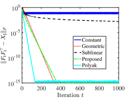
(a) $k=r$

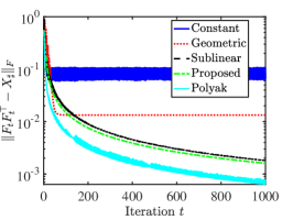
(b) $k=2r$

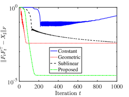
(c) $k=d$

Figure 1: Convergence of the subgradient method (3.1) with different stepsize rules in the regimes of $(a)$ exact-parameterization $k=r$, $(b)$ rank overspecication $k=2r$, and $(c)$ over-parameterization $k=d$. We use the following stepsizes: constant stepsizes $\eta_{t}=\eta_{0}$, geometric diminishing stepsizes $\eta_{t}=\eta_{0}\cdot 0.9^{t}$, sublinear diminishing stepsizes $\eta_{t}=\eta_{0}/t$, the proposed stepsizes (3.2), and the Polyaks’s stepsize.

Data generation and experiment setup.

For any given $d$ and $r$, we generate the ground truth $X_{\natural}=F_{\natural}F_{\natural}^{\top}$ with entries of $F_{\natural}\in\mathbb{R}^{d\times r}$ i.i.d. from standard normal distribution, and then normalize $X_{\natural}$ such that $\|X_{\natural}\|_{\mathrm{F}}=1$. Similarly, we generate the $m$ sensing matrices $A_{1},\ldots,A_{m}$ to be GOE matrices discussed in Section 2.1. For any given corruption ratio $p$, we generate the corruption vector $s\in\mathbb{R}^{m}$ according to the AC model, by randomly selecting $\lfloor pm\rfloor$ locations to be nonzero and generating those entries from a i.i.d. zero-mean Gaussian distribution with variance 100. We then generate the measurement according to (1.1), i.e., $y_{i}=\left\langle A_{i},X_{\natural}\right\rangle+s_{i},i=1,\dots,m$, and we set $n=100$, $p=0.2$, and $m=10nr$. We run the subgradient methods for $10^{3}$ iterations using the following different stepsizes: $(i)$ the constant stepsize $\eta_{t}=0.1$ for all $t\geq 0$, $(ii)$ sublinear diminishing stepsizes $\eta_{t}=\eta_{0}/t$, $(iii)$ geometrically diminishing stepsizes $\eta_{t}=\eta_{0}\cdot 0.9^{t}$, $(iv)$ the proposed stepsizes (3.2) with $C_{\eta}=\frac{1}{2}$, and $(v)$ the Polyak stepsize rule [34] which is given by $\eta_{t}=\frac{f(F)-f^{\star}}{\|g_{t}\|_{\mathrm{F}}^{2}}$, where $f^{\star}$ is the optimal value of (1.2) and $g_{t}$ is the subgradient in (3.1). We use the spectral initialization illustrated in Section 3.4 to generate the initialization $F_{0}$.

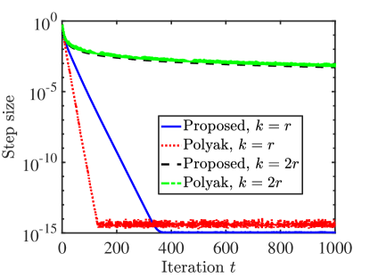
Figure 2: Comparison of the proposed stepsize in (3.2) and the Polyak stepsize in the regimes of the exact-parameterization $k=r$ and the rank overspecification $k=2r$.

Observations from the experimental results.

We run the subgradient method with different stepsize rules and different rank $k=r,\;2r,$ and $d$, and compute the reconstruction error $\|F_{t}F_{t}^{\top}-X_{\natural}\|_{\mathrm{F}}$ for the output of the algorithms. From Figure 1 and Figure 2, our observations are the follows.

• Exact rank case $k=r$. As shown in Figure 1a, we can see that (i) the subgradient method with constant stepsizes does not converge to the target matrix, (ii) using sublinear diminishing stepsizes results in a sublinear convergence rate, (iii) geometrically diminishing or Polyak stepsizes converge at a linear rate, consistent with the observation in [5], and (iv) the proposed stepsize rule also leads to convergence to the ground-truth at a linear rate, which is consistent with 3.1.

• Overspecified rank case $k=2r$. As shown in Figure 1b, the subgradient method with any stepsize rule converges at most a sublinear rate, while constant or geometrically diminishing stepsizes result in poor solution accuracy. The proposed stepsize rule achieves on par convergence performance with the sublinear stepsize rule, which also demonstrates our 3.1 on the sublinear convergence in the rank overspecified setting. As shown in Figure 2, the proposed strategy (3.2) gives stepsizes similar to Polyak’s, and thus both resulting in a similar convergence rate (or the Polyak’s is slightly better). However, the Polyak stepsize rule requires knowing the optimal value of the objective function, which is usually unknown a prior in practice.

• Overparameterized case $k=d$. The results are shown in Figure 1c. In this case, inspired by [27, 13], we use an alternative tiny initialization $F_{0}$ by drawing its entries from i.i.d. zero-mean Gaussian distribution with standard deviation $10^{-7}$. We first note that the constant stepsize rule results in overfitting. In contrast, the proposed diminishing stepsizes can prevent overfitting issues and find a very high-quality solution. We conjecture this is due to certain implicit regularization effects [26, 27, 14] and we leave thorough theoretical analysis as future work.

4.2 Robust recovery of natural images with deep image prior

Finally, we conduct an exploratory experiment on robust image recovery with DIP [16, 14]. Here, the goal is to recover a natural image $X_{\natural}$ from its corrupted measurement $y=X_{\natural}+s$, where $s$ denotes noise corruptions. To achieve this, the DIP fits the observation by a highly overparameterized deep U-Net $\phi(\Theta)$ by solving $\min_{\Theta}\|y-\phi(\Theta)\|_{\square}$ [37], where $\Theta$ denotes network parameters and the norm $\left\|\cdot\right\|_{\square}$ can be either $\ell_{2}$ or $\ell_{1}$ depending on the type of noises. As shown in [16, 32, 14], by learning the parameters $\Theta$, the network first reveals the underlying clear image and then overfits due to overparameterization, so that in many cases early stopping is crucially needed for its success.

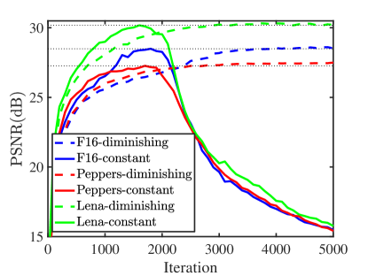
Figure 3: Learning curves for robust image recovery with DIP on different test images with 50% salt-and-pepper noise. Here, we compare the constant and diminishing stepsize rules for DIP.

In contrast to the constant stepsize rule, here we show a surprising result that, for sparse corruptions, optimizing a robust loss using the subgradient method with a diminishing stepsize rule does not overfit. In particular, we consider a sparse corruption $s$ by impulse salt-and-pepper noise, and solve the robust DIP problem $\min_{\Theta}\|y-\phi(\Theta)\|_{1}$ using the subgradient method with a diminishing stepsize rule. We test the performance using three images, “F16”, “Peppers” and “Lena” from a standard dataset [38], where we contaminate the image with salt-and-pepper noise by randomly replacing $50\%$ pixels with either $1$ or $0$ (each happens with $50\%$ probability). We compare the subgradient method with constant stepsize $0.01$ (or learning rate) and diminishing stepsize (we use an initial stepsize $0.05$ which is then scaled by $0.96$ for every $50$ iterations). As shown in Figure 3, the subgradient method with constant stepsize eventually overfits so that it requires early stopping. In comparison, optimization with diminishing stepsize prevents overfitting in the sense that the performance continues to improve as training proceeds, and it achieves on par performance with that of constant stepsizes when the learning is early stopped at the optimal PSNR. However, early stopping is not easy to implement in practice without knowing the clean image a priori.

5 Discussion

In this work, we designed and analyzed a subgradient method for the robust matrix recovery problem under the rank overspecified setting, showing that it converges to the exact solution with a sublinear rate. Based on our results, there are several directions worth further investigation.

• Better sample complexity. Our exact recovery result in Theorem 3.2 requires $\tilde{\mathcal{O}}(dk^{3})$ many samples. When the rank is exactly specified ($k=r$), for factor approaches with corrupted measurements, the best sample complexity result is $\tilde{\mathcal{O}}(dr^{2})$ [2, 4]. Hence there is an extra $k$ factor in the rank overspecified setting. Such a worse dependence may come from the $\delta^{-4}$ dependence of the sample complexity of RDPP in Proposition 2.2. More specifically, the Cauchy-Schwartz inequality we applied in (C.30) might make the dependence on $\delta$ (and hence $k$) not tight enough. We leave the improvements for future work.

• Implicit regularization. As explored and demonstrated in our experiments in Section 4, our stepsize choice combined with random initialization recovers $X_{\natural}$ with high accuracy, even if $k\geq r$ and the number of samples $m$ is way less than the degree of freedom (i.e., $m=O(dr)$). Theoretically justifying this phenomenon in the overparameterized regime would be of great interest.

• Other sensing matrix. In this work, we assume $A_{i}$ to be a GOE matrix. This specific assumption on the measurement matrix still seems to be restrictive. For other measurements such as matrices with i.i.d. sub-Gaussian entries, we believe that RDPP has to be modified. Empirically, we find that the algorithm is applicable to a broader setting (e.g., Robust PCA) even if the RDPP does not hold. Generalizing our results to more generic sensing matrices would also be an interesting future direction.

• Rectangular matrices. In this work, we utilize the fact that $X_{\natural}$ is PSD, and optimize over one factor $F$. This is consistent with much existing analysis with rank overspecification [27, 15, 13]. For rectangular $X_{\natural}$, we need to optimize over two factors $U,V$. How to combine the analysis here with an extra regularization $\|UU^{\top}-VV^{\top}\|_{\mathrm{F}}^{2}$ in the objective is another interesting direction to pursue.

Appendix A Analysis of algorithm under conditions of Theorem 3.1

To set the stage, we introduce some notations. Let the singular value decomposition of $X_{\natural}$ be

$$X_{\natural}=\begin{bmatrix}U&V\end{bmatrix}\begin{bmatrix}D_{S}^{*}&0\\ 0&0\end{bmatrix}\begin{bmatrix}U&V\end{bmatrix}^{\top},$$ (A.1)

where $U\in\mathbb{R}^{d\times r},V\in\mathbb{R}^{d\times d-r},D_{S}^{*}\in\mathbb{R}^{r\times r}$. $U$ and $V$ has orthonormal columns and $U^{\top}V=0$. Denote $\sigma_{i}$ the singular values of $X_{\natural}$, thus $\sigma_{1}$ and $\sigma_{r}$ are the largest and smallest values in $D_{S}^{*}$. Since $X_{\natural}$ is assumed to have rank $r$, we have $\sigma_{r+1}=\sigma_{r+2}=\ldots=\sigma_{d}=0$. The condition number is defined to be $\kappa=\frac{\sigma_{1}}{\sigma_{r}}$. Since union of column space of $U$ and $V$ spans the whole space, for any $F_{t}\in\mathbb{R}^{d\times r}$, we can write

$$F_{t}=US_{t}+VT_{t},$$ (A.2)

where $S_{t}=U^{\top}F_{t}\in\mathbb{R}^{r\times k}$ and $T_{t}=V^{\top}F_{t}\in\mathbb{R}^{(d-r)\times k}$.
First of all, our initialization strategy will give us the following initialization quality.

Proposition A.1 (Initialization quality).

Under the condition on $F_{0}$, we have

$$4\left\|T_{0}\right\|^{2} \leq 0.001\sigma_{r}(S_{0})\frac{\sigma_{r}}{\sqrt{\sigma_{1}}}$$ (A.3)

$$\left\|T_{0}\right\| \leq\min\{0.1\sqrt{\sigma_{1}},\frac{\sigma_{r}}{200\sqrt{\sigma_{1}}}\}=\frac{\sigma_{r}}{200\sqrt{\sigma_{1}}}$$ (A.4)

$$\left\|S_{0}\right\| \leq 2\sqrt{\sigma_{1}}.$$ (A.5)

In the analysis, we will take $c_{\rho}$ and $\rho$ such that

$$\sigma_{r}(S_{0}) =\rho$$ (A.6)

$$\left\|T_{0}\right\| \leq c_{\rho}\rho=\frac{\sigma_{r}}{200\sqrt{\sigma_{1}}}$$ (A.7)

$$\left\|S_{0}\right\| \leq 2\sqrt{\sigma_{1}}.$$ (A.8)

The parameters satisfy $4(c_{\rho}\rho)^{2}\leq 0.001\rho\frac{\sigma_{r}}{\sqrt{\sigma_{1}}}$ and $c_{\rho}\rho\leq\min\{0.1\sqrt{\sigma_{1}},\frac{\sigma_{r}}{200\sqrt{\sigma_{1}}}\}=\frac{\sigma_{r}}{200\sqrt{\sigma_{1}}}$.

By assumptin, the RDPP holds with parameters $(k+r,\sqrt{\frac{1}{2\pi}}\delta)$ and $\delta=\frac{c}{\kappa^{3}\sqrt{k}}$ for some small constant $c$ depending on $c_{3}$ in Theorem 3.1. Since the RDPP holds, let

$$\gamma_{t}=\frac{\eta_{t}\psi(F_{t}F_{t}^{\top}-X_{\natural})}{\|F_{t}F_{t}^{\top}-X_{\natural}\|_{\mathrm{F}}},\quad D_{t}\in D(F_{t}F_{t}^{\top}-X_{\natural}),$$ (A.9)

we have

$$\left\|\eta_{t}D_{t}-\gamma_{t}(F_{t}F_{t}^{\top}-X_{\natural})\right\|_{F,k+r} \leq\eta_{t}\sqrt{\frac{1}{2\pi}}\delta$$ (A.10)

$$\leq\eta_{t}\psi(F_{t}F_{t}^{\top}-X_{\natural})\delta$$ (A.11)

$$=\delta\gamma_{t}\|F_{t}F_{t}^{\top}-X_{\natural}\|_{\mathrm{F}}.$$ (A.12)

Define the following shorthand $\Delta_{t}$,

$$\Delta_{t}=\frac{\eta_{t}}{\gamma_{t}}D_{t}-(F_{t}F_{t}^{\top}-X_{\natural}).$$ (A.13)

Using that fact that the subgradient we used in algorithm 3.1 can be written as $g_{t}=D_{t}F_{t}$, we have

$$F_{t+1} =F_{t}-\gamma_{t}(F_{t}F_{t}^{\top}-X_{\natural})F_{t}+\gamma_{t}\Delta_{t}F_{t},\quad\text{and}$$ (A.14)

$$\left\|\Delta\right\| \leq\delta\|F_{t}F_{t}^{\top}-X_{\natural}\|_{\mathrm{F}}\overset{(a)}{\leq}\delta\sqrt{k+r}\left\|F_{t}F_{t}^{\top}-X_{\natural}\right\|$$ (A.15)

Here step $(a)$ is because $F_{t}F_{t}^{\top}-X_{\natural}$ has rank no more than $k+r$. Note that $\tilde{F}_{t+1}=F_{t}-\gamma_{t}\left(F_{t}F_{t}^{\top}-X_{\natural}\right)F_{t}$ is the update if we apply gradient descent to smooth function $\tilde{f}(F)=\frac{1}{4}\|FF^{\top}-X_{\natural}\|_{\mathrm{F}}^{2}$. We will leverage the properties of this population level update throughout the analysis. The next proposition illustrates the evolution of $S_{t}$ and $T_{t}$.

Proposition A.2 (Updates of $S_{t},T_{t}$).

For any $t\geq 0$, we have

$$S_{t+1} =S_{t}-\gamma_{t}\left(S_{t}S_{t}^{\top}S_{t}+S_{t}T_{t}^{\top}T_{t}-D_{S}^{*}S_{t}\right)+\gamma_{t}U^{\top}\Delta_{t}F_{t},$$ (A.16)

$$T_{t+1} =T_{t}-\gamma_{t}\left(T_{t}T_{t}^{\top}T_{t}+T_{t}S_{t}^{\top}S_{t}\right)+\gamma_{t}V^{\top}\Delta_{t}F_{t}.$$ (A.17)

We introduce notations

$$\mathcal{M}_{t}(S_{t}) =S_{t}-\gamma_{t}\left(S_{t}S_{t}^{\top}S_{t}+S_{t}T_{t}^{\top}T_{t}-D_{S}^{*}S_{t}\right)$$ (A.18)

$$\mathcal{N}_{t}(T_{t}) =T_{t}-\gamma_{t}\left(T_{t}T_{t}^{\top}T_{t}+T_{t}S_{t}^{\top}S_{t}\right).$$ (A.19)

They are "population-level" updates for $S_{t}$ and $T_{t}$.

Proposition A.3 (Uniform upper bound).

Suppose $\gamma_{t}$ satisfies $\gamma_{t}\leq\frac{0.01}{\sigma_{1}}$ for all $t\geq 0$ and $(50\sqrt{k}\delta)^{\frac{1}{3}}\leq\frac{c_{\rho}\rho}{2\sqrt{\sigma_{1}}}=\frac{\sigma_{r}}{400\sigma_{1}}$, we have

$$\left\|T_{t}\right\| \leq c_{\rho}\rho\leq 0.1\sqrt{\sigma_{r}}\leq 0.1\sqrt{\sigma_{1}}$$ (A.20)

$$\left\|S_{t}\right\| \leq 2\sqrt{\sigma_{1}}$$ (A.21)

for all $t\geq 0$.

The analysis of algorithm consists of three stages:

• In stage $1$, we show at $\sigma_{r}(S_{t})$ increases geometrically to level $\sqrt{\frac{\sigma_{r}}{2}}$ by time $\mathcal{T}_{1}^{\prime}$, then $\left\|S_{t}S_{t}^{\top}-D_{S}^{*}\right\|$ will decrease geometrically to $\frac{100(c_{\rho}\rho)^{2}\sigma_{1}}{\sigma_{r}}(\leq\frac{\sigma_{r}}{100})$by $\mathcal{T}_{1}$. The iterate will then enter a good region.

• In stage $2$, we show that $D_{t}=\max\{\left\|S_{t}S_{t}^{\top}-D_{S}^{*}\right\|,\left\|S_{t}T_{t}^{\top}\right\|\}$ decreases geometrically if it is bigger than $10\delta\sqrt{2k}\sigma_{1}$, which is the computational threshold. In other words, $\left\|S_{t}S_{t}^{\top}-D_{S}^{*}\right\|$ decrease to a $\frac{100(c_{\rho}\rho)^{2}\sigma_{1}}{\sigma_{r}}$ geometrically, and this will happen by $\mathcal{T}_{2}$.

• In stage $3$, after $\mathcal{T}_{2}$, $E_{t}=\max\{\left\|S_{t}S_{t}^{\top}-D_{S}^{*}\right\|,\left\|S_{t}T_{t}^{\top}\right\|,\left\|T_{t}T_{t}^{\top}\right\|\}$ converges to $0$ sublinearly.

In the above statement,

$$\mathcal{T}_{1}^{\prime}=\left\lceil\log\left(\frac{\sqrt{\sigma_{r}}}{\sqrt{2}\rho}\right)/\log\left(1+\frac{c_{\gamma}\sigma_{r}^{2}}{6\sigma_{1}^{2}}\right)\right\rceil,$$ (A.22)

$$\mathcal{T}_{1}=\mathcal{T}_{1}^{\prime}+\left\lceil\frac{\log(\frac{20(c_{\rho}\rho)^{2}}{\sigma_{r}})}{\log\left(1-\frac{c_{\gamma}\sigma_{r}^{2}}{2\sigma_{1}^{2}}\right)}\right\rceil$$ (A.23)

and

$$\mathcal{T}_{2}=\mathcal{T}_{1}+\left\lceil\frac{\log\left(\frac{1000\delta\sqrt{k}\sigma_{1}}{\sigma_{r}}\right)}{\log\left(1-\frac{c_{\gamma}\sigma_{r}^{2}}{6\sigma_{1}^{2}}\right)}\right\rceil.$$ (A.24)

Stage $1$ consists of all the iterations up to time $\mathcal{T}_{1}$. Stage $2$ consists of all the iterations between $\mathcal{T}_{1}+1$ and $\mathcal{T}_{2}$. Stage $3$ consists of all the iterations afterwards.

A.1 Analysis of $\mathcal{M}_{t}(S_{t})$ and $\mathcal{N}_{t}(T_{t})$.

In this sections we prove some facts about $\mathcal{M}_{t}(S_{t})$ and $\mathcal{N}_{t}(T_{t})$ that will be useful in the analysis.

Proposition A.4.

Suppose $\gamma_{t}\leq\min\{\frac{0.01}{\sigma_{1}},\frac{0.01\sigma_{r}}{\sigma_{1}^{2}}\}$, $\left\|S_{t}\right\|\leq 2\sqrt{\sigma_{1}}$, $\sigma_{r}(S_{t})\geq\sqrt{\frac{\sigma_{r}}{2}}$ and $\left\|T_{t}\right\|\leq 0.1\sqrt{\sigma_{r}}$, we have the following:

1. $\left\|\mathcal{M}_{t}(S_{t})\mathcal{M}_{t}(S_{t})^{\top}-D^{*}_{S}\right\|\leq(1-\frac{3\gamma_{t}\sigma_{r}}{4})\left\|S_{t}S_{t}^{\top}-D_{S}^{*}\right\|+3\gamma_{t}\left\|S_{t}T_{t}^{\top}\right\|^{2}$.

Suppose $\gamma_{t}\leq\frac{0.01}{\sigma_{1}}$, $\left\|S_{t}\right\|\leq 2\sqrt{\sigma_{1}}$, and $\left\|T_{t}\right\|\leq 0.1\sqrt{\sigma_{r}}$, we have the following:

1. $\left\|\mathcal{N}_{t}(T_{t})\mathcal{N}_{t}(T_{t})^{\top}\right\|\leq\left\|T_{t}\right\|^{2}(1-\frac{3\gamma_{t}}{2}\left\|T_{t}\right\|^{2})=\left\|T_{t}T_{t}^{\top}\right\|\left(1-\frac{3\gamma_{t}}{2}\left\|T_{t}T_{t}^{\top}\right\|\right)$.

Furthermore, suppose $\gamma_{t}\leq\frac{0.01}{\sigma_{1}}$, $\left\|S_{t}\right\|\leq 2\sqrt{\sigma_{1}}$, $\sigma_{r}(S_{t})\geq\sqrt{\frac{\sigma_{r}}{2}}$, $\left\|T_{t}\right\|\leq 0.1\sqrt{\sigma_{r}}$, and $\left\|S_{t}S_{t}^{\top}-D_{S}^{*}\right\|\leq\frac{\sigma_{r}}{10}$, we have same inequalities as $1$, $2$ and

1. $\left\|\mathcal{M}_{t}(S_{t})\mathcal{N}_{t}(T_{t})^{\top}\right\|\leq(1-\frac{\gamma_{t}\sigma_{r}}{3})\left\|S_{t}T_{t}^{\top}\right\|$.

Proposition A.5.

Suppose $\gamma_{t}\leq\frac{0.01}{\sigma_{1}}$, $\left\|S_{t}\right\|\leq 2\sqrt{\sigma_{1}}$, $\sigma_{r}(S_{t})\geq\sqrt{\frac{\sigma_{r}}{2}}$ and $\left\|T_{t}\right\|\leq 0.1\sqrt{\sigma_{r}}$, we have the following:

1. $\left\|D_{S}^{*}-\mathcal{M}_{t}(S_{t})S_{t}^{\top}\right\|\leq\left(1-\frac{\gamma\sigma_{r}}{2}\right)\left\|D_{S}^{*}-S_{t}S_{t}^{\top}\right\|+\gamma_{t}\left\|S_{t}T_{t}^{\top}\right\|^{2}$.

2. $\left\|\mathcal{M}_{t}(S_{t})T_{t}^{\top}\right\|\leq 2\left\|S_{t}T_{t}^{\top}\right\|$.

3. $\left\|\mathcal{N}_{t}(T_{t})S_{t}^{\top}\right\|\leq\left\|T_{t}S_{t}^{\top}\right\|$.

4. $\left\|\mathcal{N}_{t}(T_{t})T_{t}^{\top}\right\|\leq\left\|T_{t}\right\|^{2}(1-\gamma_{t}\left\|T_{t}\right\|^{2})=\left\|T_{t}T_{t}^{\top}\right\|\left(1-\gamma_{t}\left\|T_{t}T_{t}^{\top}\right\|\right).$

A.2 Analysis of Stage 1

The following proposition characterize the evolution of $\sigma_{r}(S_{t})$. In stage one, we start with a initialization satisfies conditions in Proposition A.1.

Proposition A.6.

Suppose there is some constant $c_{\gamma}>0$ such that the parameters satisfy $\frac{c_{\gamma}\sigma_{r}}{\sigma_{1}^{2}}\leq\gamma_{t}\leq\min\{\frac{1}{100\sigma_{1}},\frac{\sigma_{r}}{100\sigma_{1}^{2}}\}=\frac{\sigma_{r}}{100\sigma_{1}^{2}}$, $(50\sqrt{k}\delta)^{\frac{1}{3}}\leq\frac{c_{\rho}\rho}{2\sqrt{\sigma_{1}}}=\frac{\sigma_{r}}{400\sigma_{1}}$, we have

$$\sigma_{r}(S_{t})\geq\min\left\{(1+\frac{\sigma_{r}^{2}c_{\gamma}}{6\sigma_{1}^{2}})^{t}\sigma_{r}(S_{0}),\sqrt{\frac{\sigma_{r}}{2}}\right\}$$ (A.25)

for all $t\geq 0$. In particular, we have

$$\sigma_{r}(S_{\mathcal{T}_{1}^{\prime}}+t) \geq\sqrt{\frac{\sigma_{r}}{2}}.$$ (A.26)

for all $t\geq 0$.

Next, we show that $\left\|S_{t}S_{t}^{\top}-D_{S}^{*}\right\|$ decays geometrically to $\frac{100(c_{\rho}\rho)^{2}\sigma_{1}}{\sigma_{r}}$.

Proposition A.7.

Suppose there is some constant $c_{\gamma}>0$ such that the parameters satisfy $\frac{c_{\gamma}\sigma_{r}}{\sigma_{1}^{2}}\leq\gamma_{t}\leq\min\{\frac{1}{100\sigma_{1}},\frac{\sigma_{r}}{100\sigma_{1}^{2}}\}=\frac{\sigma_{r}}{100\sigma_{1}^{2}}$, $(50\sqrt{k}\delta)^{\frac{1}{3}}\leq\frac{c_{\rho}\rho}{2\sqrt{\sigma_{1}}}$, we have for any $t\geq 0$, we have

$$\left\|S_{\mathcal{T}_{1}+t}S_{\mathcal{T}_{1}+t}^{\top}-D_{S}^{*}\right\|\leq\max\{5\sigma_{1}(1-\frac{c_{\gamma}\sigma_{r}^{2}}{2\sigma_{1}^{2}})^{t},\frac{100(c_{\rho}\rho)^{2}\sigma_{1}}{\sigma_{r}}\}.$$ (A.27)

In particular, for $\mathcal{T}_{1}=\mathcal{T}_{1}^{\prime}+\left\lceil\frac{\log(\frac{20(c_{\rho}\rho)^{2}}{\sigma_{r}})}{\log\left(1-\frac{c_{\gamma}\sigma_{r}^{2}}{2\sigma_{1}^{2}}\right)}\right\rceil$, we have

$$\left\|S_{t}S_{t}^{\top}-D_{S}^{*}\right\|\leq\frac{100(c_{\rho}\rho)^{2}\sigma_{1}}{\sigma_{r}}\leq\frac{\sigma_{r}}{100},\qquad\forall t\geq\mathcal{T}_{1}.$$ (A.28)

When $t=\mathcal{T}_{1}$, by Proposition A.7,

$$\left\|D_{S}^{*}-S_{\mathcal{T}_{1}}S_{\mathcal{T}_{1}}^{\top}\right\|\leq\frac{\sigma_{r}}{100}.$$ (A.29)

By Proposition A.3 and our assumption that $c_{\rho}\rho\leq\frac{\sigma_{r}}{200\sqrt{\sigma_{1}}}$,

$$\left\|S_{\mathcal{T}_{1}}T_{\mathcal{T}_{1}}\right\|\leq 2(c_{\rho}\rho)\sqrt{\sigma_{1}}\leq\frac{\sigma_{r}}{100}.$$ (A.30)

Combining, we obtain

$$D_{\mathcal{T}_{1}}\leq\frac{\sigma_{r}}{100}.$$ (A.31)

A.3 Analysis of Stage 2

Recall

$$D_{t}=\max\{\left\|S_{t}S_{t}^{\top}-D_{S}^{*}\right\|,\left\|S_{t}T_{t}^{\top}\right\|\}.$$ (A.32)

We show that $D_{t}$ decreases to $10\delta\sqrt{k+r}\sigma_{1}$ geometrically after $\mathcal{T}_{1}$.

Proposition A.8.

Suppose there is some constant $c_{\gamma}>0$ such that the parameters satisfy $\frac{c_{\gamma}\sigma_{r}}{\sigma_{1}^{2}}\leq\gamma_{t}\leq\frac{0.01}{\sigma_{1}}$, $\delta\sqrt{k+r}\leq\frac{0.001\sigma_{r}}{\sigma_{1}}$. Also, we suppose $\left\|T_{t}\right\|\leq 0.1\sqrt{\sigma_{r}}$ for all $t$. If for some $\mathcal{T}_{1}>0$,

$$D_{\mathcal{T}_{1}}\leq\max\{\frac{\sigma_{r}}{100},10\delta\sqrt{k+r}\sigma_{1}\}=\frac{\sigma_{r}}{100},$$ (A.33)

then for any $t\geq 0$, we have

$$D_{\mathcal{T}_{1}+t}\leq\max\left\{\left(1-\frac{c_{\gamma}\sigma_{r}^{2}}{6\sigma_{1}^{2}}\right)^{t}\cdot\frac{\sigma_{r}}{100},10\delta\sqrt{k+r}\sigma_{1}\right\}.$$ (A.34)

In particular, for $\mathcal{T}_{2}=\mathcal{T}_{1}+\left\lceil\frac{\log\left(\frac{1000\delta\sqrt{k+r}\sigma_{1}}{\sigma_{r}}\right)}{\log\left(1-\frac{c_{\gamma}\sigma_{r}^{2}}{6\sigma_{1}^{2}}\right)}\right\rceil$, we have

$$\left\|S_{t}S_{t}^{\top}-D_{S}^{*}\right\| \leq 10\delta\sqrt{k+r}\sigma_{1},$$ (A.35)

$$\left\|S_{t}T_{t}^{\top}\right\| \leq 10\delta\sqrt{k+r}\sigma_{1},\qquad\forall t\geq\mathcal{T}_{2}.$$ (A.36)

A.4 Analysis of Stage 3

Define

$$E_{t}=\max\{\left\|S_{t}S_{t}^{\top}-D_{S}^{*}\right\|,\left\|S_{t}T_{t}^{\top}\right\|,\left\|T_{t}T_{t}^{\top}\right\|\}.$$ (A.37)

We are going to show the sublinear convergence of $E_{t}$ in stage three.

Proposition A.9.

Suppose we have $\gamma_{t}\leq\frac{0.01}{\sigma_{1}}$, $\delta\sqrt{k+r}\leq\frac{0.001\sigma_{r}}{\sigma_{1}}$ and $E_{t}\leq 0.01\sigma_{r}$ for some $t>0$. Then we have

$$E_{t+1}\leq\max\{(1-\frac{\gamma_{t}\sigma_{r}}{6})E_{t},E_{t}(1-\gamma_{t}E_{t})\}=E_{t}(1-\gamma_{t}E_{t}).$$ (A.38)

Indeed, we can prove a better rate if there is no overparametrization.

Proposition A.10.

Suppose we have $\gamma_{t}\leq\frac{0.01}{\sigma_{1}}$, $\delta\sqrt{k+r}\leq\frac{0.001\sigma_{r}}{\sigma_{1}}$ and $E_{t}\leq 0.01\sigma_{r}$ for some $t>0$. If $k=r$, then we have

$$E_{t+1}\leq(1-\frac{\gamma_{t}\sigma_{r}}{3})E_{t}.$$ (A.39)

A.5 Proof of Theorem 3.1

The proof is a combination of all the propositions in this section. First, we show that under suitable choice of $c_{0}$ and $c_{3}$, all the assumptions are satisfied. First, if we take $c_{3}$ to be small enough, we know that $(50\sqrt{k}\delta)^{\frac{1}{3}}\leq\frac{\sigma_{r}}{400\sigma_{1}}$ holds. Hence, all the conditions related to $\delta$ are satisfied. Next, by definition, $\gamma_{t}=\frac{\eta_{t}\psi(F_{t}F_{t}^{\top}-X_{\natural})}{\|F_{t}F_{t}^{\top}-X_{\natural}\|_{\mathrm{F}}}$. By the second assumption and the assumption on range of $\psi$, we know

$$\gamma_{t}\in[c_{1}\sqrt{\frac{1}{2\pi}}\frac{\sigma_{r}}{\sigma_{1}^{2}},c_{2}\sqrt{\frac{2}{\pi}}\frac{\sigma_{r}}{\sigma_{1}^{2}}].$$ (A.40)

Since we assumed $c_{2}\leq 0.01$, so the step size condition $\gamma_{t}\leq\frac{\sigma_{r}}{100\sigma_{1}^{2}}$ is satisfied. Moreover, $c_{\gamma}\geq c_{1}\sqrt{\frac{1}{2\pi}}$. Now, applying theorems for initialization, stage 1 and stage 2, we know that

$$\left\|S_{\mathcal{T}_{2}}S_{\mathcal{T}_{2}}^{\top}-D_{S}^{*}\right\| \leq 10\delta\sqrt{k+r}\sigma_{1}\leq\frac{0.01\sigma_{r}^{2}}{\sigma_{1}},$$ (A.41)

$$\left\|S_{\mathcal{T}_{2}}T_{\mathcal{T}_{2}}^{\top}\right\| \leq 10\delta\sqrt{k+r}\sigma_{1}\leq\frac{0.01\sigma_{r}^{2}}{\sigma_{1}}.$$ (A.42)

In addition, by Proposition A.3, we know

$$\left\|T_{\mathcal{T}_{2}}T_{\mathcal{T}_{2}}^{\top}\right\|=\left\|T_{\mathcal{T}_{2}}\right\|^{2}\leq(c_{\rho}\rho)^{2}\leq\frac{0.01\sigma_{r}^{2}}{\sigma_{1}}.$$ (A.43)

Hence, $E_{\mathcal{T}_{2}}\leq\frac{0.01\sigma_{r}^{2}}{\sigma_{1}}$. Here are two cases:

• $k>r$, By Proposition A.9 and induction, we know

  $$E_{t+1}\leq E_{t}(1-\gamma_{t}E_{t})\leq E_{t}(1-\frac{c_{\gamma}\sigma_{r}}{\sigma_{1}^{2}}E_{t}),\qquad\forall t\geq\mathcal{T}_{2}.$$ (A.44)

  where $c_{1}\sqrt{\frac{2}{\pi}}\leq c_{\gamma}\leq 0.01$. Define $G_{t}=\frac{c_{\gamma}\sigma_{r}}{\sigma_{1}^{2}}E_{t}$, then we have $G_{\tau_{2}}<1$ and

  $$G_{t+1}\leq G_{t}(1-G_{t}),\qquad\forall t\geq\mathcal{T}_{2}.$$ (A.45)

  Taking reciprocal, we obtain

  $$\frac{1}{G_{t+1}}\geq\frac{1}{G_{t}}+\frac{1}{1-G_{t}}\geq\frac{1}{G_{t}}+1,\qquad\forall t\geq\mathcal{T}_{2}$$ (A.46)

  So we obtain

  $$G_{\mathcal{T}_{2}+t}\leq\frac{1}{\frac{1}{G_{\mathcal{T}_{2}}}+t},\qquad\forall t\geq 0.$$ (A.47)

  Plugging in the definition of $G_{t}$, we obtain

  $$E_{\tau_{2}+t}\leq\frac{\sigma_{1}^{2}}{c_{\gamma}\sigma_{r}}\frac{1}{\frac{\sigma_{1}^{2}}{c_{\gamma}\sigma_{r}E_{\mathcal{T}_{2}}}+t}\leq\frac{\sigma_{1}^{2}}{c_{\gamma}\sigma_{r}}\frac{1}{\frac{100\sigma_{1}^{3}}{c_{\gamma}\sigma_{r}^{3}}+t}=\frac{\sigma_{1}}{c_{\gamma}}\frac{\kappa}{\frac{100}{c_{\gamma}}\kappa^{3}+t}\leq\frac{\sigma_{1}}{c_{\gamma}}\frac{\kappa}{\kappa^{3}+t}.$$ (A.48)

  Since $c_{\gamma}\geq c_{1}\sqrt{\frac{2}{\pi}}$, we can simply take $c_{5}=\frac{1}{4c_{1}}\sqrt{\frac{\pi}{2}}$, $\mathcal{T}=\mathcal{T}_{2}$, apply Lemma I.5, and get

  $$\left\|F_{\mathcal{T}+t}F_{\mathcal{T}+t}^{\top}-X_{\natural}\right\|\leq c_{5}\sigma_{1}\frac{\kappa}{\kappa^{3}+t},\qquad\forall t\geq 0.$$ (A.49)

  The last thing to justify is $\mathcal{T}_{2}\lesssim\kappa^{2}\log\kappa$. Recall

  $$\mathcal{T}_{1}^{\prime}=\left\lceil\log\left(\frac{\sqrt{\sigma_{r}}}{\sqrt{2}\rho}\right)/\log\left(1+\frac{c_{\gamma}\sigma_{r}^{2}}{6\sigma_{1}^{2}}\right)\right\rceil,$$ (A.50)

  $$\mathcal{T}_{1}=\mathcal{T}_{1}^{\prime}+\left\lceil\frac{\log(\frac{20(c_{\rho}\rho)^{2}}{\sigma_{r}})}{\log\left(1-\frac{c_{\gamma}\sigma_{r}^{2}}{2\sigma_{1}^{2}}\right)}\right\rceil$$ (A.51)

  and

  $$\mathcal{T}_{2}=\mathcal{T}_{1}+\left\lceil\frac{\log\left(\frac{1000\delta\sqrt{k}\sigma_{1}}{\sigma_{r}}\right)}{\log\left(1-\frac{c_{\gamma}\sigma_{r}^{2}}{6\sigma_{1}^{2}}\right)}\right\rceil.$$ (A.52)

  Simple calculus yield that each integer above is $O(\kappa^{2}\log\kappa)$. So the proof is complete in overspecified case.

• $k=r$. By Proposition A.10 and induction, we obtain

  $$E_{t+1}\leq(1-\frac{\gamma_{t}\sigma_{r}}{3})E_{t}\leq(1-\frac{c_{\gamma}\sigma_{r}^{2}}{\sigma_{1}^{2}})E_{t},\forall t\geq\mathcal{T}_{2}.$$ (A.53)

  Applying this inequality recursively and noting $c_{\gamma}\geq c_{1}\sqrt{\frac{2}{\pi}}$, we obtain

  $$E_{\mathcal{T}_{2}+t}\leq(1-\frac{c_{\gamma}\sigma_{r}^{2}}{\sigma_{1}^{2}})^{t}E_{\mathcal{T}_{2}}\leq\left(1-\frac{c_{1}\sqrt{\frac{2}{\pi}}}{\kappa^{2}}\right)^{t}\frac{0.01\sigma_{r}}{\kappa},\forall t\geq 0.$$ (A.54)

  Thus, we can take $c_{6}=0.01/4$, $c_{7}=c_{1}\sqrt{\frac{2}{\pi}}$, $\mathcal{T}=\mathcal{T}_{2}$, apply Lemma I.5 and get

  $$\left\|F_{\mathcal{T}+t}F_{\mathcal{T}+t}^{\top}-X_{\natural}\right\|\leq\frac{c_{6}\sigma_{r}}{\kappa}\left(1-\frac{c_{7}}{\kappa^{2}}\right)^{t},\qquad\forall t\geq 0.$$ (A.55)

  The validity of $\mathcal{T}$ is proved in the last part. The proof is complete.

Appendix B Proof of Propositions

B.1 Proof of Proposition A.1

First, we note that the $r$-th singular value of $c^{*}X_{\natural}$ is at least $\epsilon\sigma_{r}$. By almost the same proof as Lemma I.5, we get

$$\max\{\left\|S_{0}S_{0}^{\top}-c^{*}D_{S}^{*}\right\|,\left\|S_{0}T_{0}^{\top}\right\|,\left\|T_{0}T_{0}^{\top}\right\|\}\leq\left\|F_{0}F_{0}^{\top}-c^{*}X_{\natural}\right\|\leq\frac{\tilde{c}_{0}\epsilon\sigma_{r}}{\kappa}.$$ (B.1)

We take $\tilde{c}_{0}=\left(\frac{1}{200}\right)^{2}$. By Weyl’s inequality (I.3),

$$\sigma_{r}(S_{0}S_{0}^{\top})\geq\sigma_{r}(c^{*}D_{S}^{*})-\left\|S_{0}S_{0}^{\top}-c^{*}D_{S}^{*}\right\|\geq\frac{c^{*}\sigma_{r}}{4}\geq\frac{\epsilon\sigma_{r}}{4}.$$ (B.2)

Hence, $\rho=\sigma_{r}(S_{0})\geq\frac{\sqrt{\epsilon\sigma_{r}}}{2}$. On the other hand,

$$\left\|T_{0}\right\| \leq\sqrt{\frac{\tilde{c}_{0}\epsilon\sigma_{r}}{\kappa}}$$ (B.3)

$$\leq\frac{\sigma_{r}}{200\sqrt{\sigma_{1}}}$$ (B.4)

We can simply assume $\sigma_{1}(S_{0})\leq 2\sqrt{\sigma_{1}}$. If not so, we can normalize $F_{0}$ so that $\sigma_{1}(S_{0})=2\sqrt{\sigma_{1}}$ and use normalized $F_{0}$ as our initialization. By Weyl’s inequality (I.3),

$$\sigma_{1}(S_{0}S_{0}^{\top})\leq 1.01c^{*}\sigma_{1}.$$ (B.5)

Hence, $c^{*}\geq 3$. In this case, the factor we use to normalize $S_{0}$ is propotional to $c^{*}\geq 3$. It’s easy to show that $\rho=\sigma_{r}(S_{0})\geq\frac{\sqrt{\epsilon\sigma_{r}}}{2}$ and $\left\|T_{0}\right\|\leq\frac{\sigma_{r}}{200\sqrt{\sigma_{1}}}$ still holds. Therefore, the initialization quality is proved.

B.2 Proof of Proposition A.2

The algorithm A.14 updates $F_{t}$ by

$$F_{t+1}=F_{t}-\gamma_{t}\left(F_{t}F_{t}^{\top}-X_{\natural}\right)F_{t}+\gamma_{t}\Delta_{t}F_{t}.$$ (B.6)

Using the definition of $U,V,S_{t},T_{t}$, we have

$$S_{t+1} =U^{\top}F_{t+1}$$

$$=U^{\top}F_{t}-\gamma_{t}U^{\top}\left(F_{t}F_{t}^{\top}-X_{\natural}\right)F_{t}+\gamma_{t}U^{\top}\Delta_{t}F_{t}$$

$$=U^{\top}(US_{t}+VT_{t})-\gamma_{t}U^{\top}\left[(US_{t}+VT_{t})(US_{t}+VT_{t})^{\top}-UD^{*}_{S}U^{\top}-VD^{*}_{T}V^{\top}\right](US_{t}+VT_{t})$$

$$\qquad+\gamma_{t}U^{\top}\Delta_{t}F_{t}$$

$$\overset{(\sharp)}{=}S_{t}-\gamma_{t}(S_{t}S_{t}^{\top}S_{t}+S_{t}T_{t}^{\top}T_{t}-D_{S}^{*}S_{t})+\gamma_{t}U^{\top}\Delta_{t}F_{t}.$$

Here $(\sharp)$ follows from the fact that $U^{\top}V=0$ and $U,V$ are orthonormal.
By the same token, we can show

$$T_{t+1}=T_{t}-\gamma_{t}\left(T_{t}T_{t}^{\top}T_{t}+T_{t}S_{t}^{\top}S_{t}\right)+\gamma_{t}V^{\top}\Delta_{t}F_{t}.$$ (B.7)

B.3 Proof of Proposition A.3

We prove the proposition by induction. By Proposition A.1, it’s clear that the proposition holds for $t=0$. Suppose for $t\geq 0$, we have

$$\left\|T_{t}\right\| \leq c_{\rho}\rho\leq 0.1\sqrt{\sigma_{1}}$$ (B.8)

$$\left\|S_{t}\right\| \leq 2\sqrt{\sigma_{1}}.$$ (B.9)

By Proposition A.2, we know

$$S_{t+1}=S_{t}-\gamma_{t}(S_{t}S_{t}^{\top}S_{t}+S_{t}T_{t}^{\top}T_{t}-D_{S}^{*}S_{t})+\gamma_{t}U^{\top}\Delta_{t}F_{t}.$$ (B.10)

Since $\|T_{t}\|\leq c_{\rho}\rho\leq 0.1\sqrt{\sigma_{1}}$, $\|S_{t}\|\leq 2\sqrt{\sigma_{1}}$ and our assumption that $\gamma_{t}\leq\frac{0.01}{\sigma_{1}}$, $I-\gamma_{t}S_{t}^{\top}S_{t}-\gamma_{t}T_{t}^{\top}T_{t}$ is a PSD matrix. By lemma I.2,

$$\left\|S_{t}\left(I-\gamma_{t}S_{t}^{\top}S_{t}-\gamma_{t}T_{t}^{\top}T_{t}\right)\right\| \leq\left\|S_{t}\left(I-\gamma_{t}S_{t}^{\top}S_{t}\right)\right\|+\gamma_{t}\left\|S_{t}\right\|\left\|T_{t}\right\|^{2}$$ (B.11)

$$=\left\|S_{t}\right\|-\gamma_{t}\left\|S_{t}\right\|^{3}+0.1\gamma_{t}\sigma_{1}^{\frac{3}{2}}.$$ (B.12)

On the other hand, simple triangle inequality yields

$$\left\|F_{t}\right\|=\left\|US_{t}+VT_{t}\right\|\leq\left\|S_{t}\right\|+\left\|T_{t}\right\|\leq 3\sqrt{\sigma_{1}}.$$ (B.13)

By A.15 and lemma I.4, we get

$$\left\|\Delta_{t}F_{t}\right\| \leq\left\|\Delta_{t}\right\|\left\|F_{t}\right\|$$ (B.14)

$$\leq 3\sigma_{1}^{\frac{1}{2}}\delta\|F_{t}F_{t}^{\top}-X_{\natural}\|_{\mathrm{F}}$$ (B.15)

$$\leq 3\sigma_{1}^{\frac{1}{2}}\delta\sqrt{k+r}\left\|F_{t}F_{t}^{\top}-X_{\natural}\right\|$$ (B.16)

$$\leq 3\sigma_{1}^{\frac{1}{2}}\delta\sqrt{k+r}\left(\left\|F_{t}\right\|^{2}+\left\|X_{\natural}\right\|\right)$$ (B.17)

$$\leq 50\delta\sqrt{k}\sigma_{1}^{\frac{3}{2}}$$ (B.18)

$$\leq 0.1\sigma_{1}^{\frac{3}{2}}$$ (B.19)

Combining, we have

$$\left\|S_{t+1}\right\| \leq\left\|S_{t}\left(I-\gamma_{t}S_{t}^{\top}S_{t}-\gamma_{t}T_{t}^{\top}T_{t}\right)\right\|+\gamma_{t}\left\|D_{S}^{*}S_{t}\right\|+\gamma_{t}\left\|U^{\top}\Delta_{t}F_{t}\right\|$$ (B.20)

$$\leq\left\|S_{t}\right\|-\gamma_{t}\left\|S_{t}\right\|^{3}+\gamma_{t}\sigma_{1}\left\|S_{t}\right\|+0.2\gamma_{t}\sigma_{1}^{\frac{3}{2}}$$ (B.21)

$$=\left\|S_{t}\right\|\left(1+\gamma_{t}\sigma_{1}-\gamma_{t}\left\|S_{t}\right\|^{2}\right)+0.2\gamma_{t}\sigma_{1}^{\frac{3}{2}}.$$ (B.22)

We consider two different cases:

• $\|S_{t}\|\leq 1.5\sqrt{\sigma_{1}}$. By the inequality above, we have

  $$\left\|S_{t+1}\right\|\leq\left\|S_{t}\right\|(1+\gamma_{t}\sigma_{1})+0.1\gamma_{t}\sigma_{1}^{\frac{3}{2}}\leq 1.6\sqrt{\sigma_{1}}+0.2\sqrt{\sigma_{1}}\leq 2\sqrt{\sigma_{1}}$$ (B.23)

• $1.5\sqrt{\sigma_{1}}<\|S_{t}\|\leq 2\sqrt{\sigma_{1}}$. In this case, we have

  $$\left\|S_{t+1}\right\| \leq\left\|S_{t}\right\|(1+\gamma_{t}\sigma_{1}-2.25\gamma_{t}\sigma_{1})+0.2\gamma_{t}\sigma_{1}^{\frac{3}{2}}$$ (B.24)

  $$\leq\left\|S_{t}\right\|(1-\gamma_{t}\sigma_{1})+0.2\gamma_{t}\sigma_{1}\left\|S_{t}\right\|$$ (B.25)

  $$\leq\left\|S_{t}\right\|$$ (B.26)

  $$\leq 2\sqrt{\sigma_{1}}.$$ (B.27)

The desired bound for $S_{t+1}$ is established. For $T_{t+1}$, we note

$$T_{t+1}=T_{t}(I-\gamma_{t}T_{t}^{\top}T_{t}-\gamma_{t}S_{t}^{\top}S_{t})+\gamma_{t}V^{\top}\Delta_{t}F_{t}.$$ (B.28)

We expand $T_{t+1}T_{t+1}^{\top}$ and obtain

$$T_{t+1}T_{t+1}^{\top} =(\mathcal{N}_{t}(T_{t})+\gamma_{t}V^{\top}\Delta_{t}F_{t})(\mathcal{N}_{t}(T_{t})+\gamma_{t}V^{\top}\Delta_{t}F_{t})^{\top}$$ (B.29)

$$\leq\underbrace{\mathcal{N}_{t}(T_{t})\mathcal{N}_{t}(T_{t})^{\top}}_{Z_{1}}+\underbrace{\gamma_{t}V^{\top}\Delta_{t}F_{t}\mathcal{N}_{t}(T_{t})^{\top}+\gamma_{t}\mathcal{N}_{t}(T_{t})F_{t}^{\top}\Delta_{t}^{\top}V}_{Z_{2}}$$ (B.30)

$$\qquad+\underbrace{\gamma_{t}^{2}V^{\top}\Delta_{t}F_{t}F_{t}^{\top}\Delta_{t}^{\top}V}_{Z_{3}}$$ (B.31)

By Proposition A.4, we have $\|Z_{1}\|\leq\|T_{t}T_{t}^{\top}\|(1-\frac{3\gamma_{t}}{2}\|T_{t}T_{t}^{\top}\|).$ By induction hypothesis and triangle inequality, we have

$$\left\|Z_{2}\right\| \leq 2\gamma_{t}50\delta\sqrt{k}\sigma_{1}^{\frac{3}{2}}\|\mathcal{N}_{t}(T_{t})\|$$ (B.32)

$$\leq 2\gamma_{t}50\delta\sqrt{k}\sigma_{1}^{\frac{3}{2}}\|T_{t}\|$$ (B.33)

and

$$\left\|Z_{3}\right\|\leq\gamma_{t}^{2}\left(50\delta\sqrt{k}\sigma_{1}^{\frac{3}{2}}\right)^{2}\leq 0.01\gamma_{t}(c_{\rho}\rho)^{4}.$$ (B.34)

By triangle inequality, we have

$$\left\|T_{t+1}T_{t+1}^{\top}\right\| \leq\|Z_{1}\|+\|Z_{2}\|+\|Z_{3}\|$$ (B.35)

$$\leq\|T_{t}T_{t}^{\top}\|(1-\frac{3\gamma_{t}}{2}\|T_{t}T_{t}^{\top}\|)+2\gamma_{t}50\delta\sqrt{k}\sigma_{1}^{\frac{3}{2}}\|T_{t}\|+0.01\gamma_{t}(c_{\rho}\rho)^{4}$$ (B.36)

We consider two different cases:

• $\left\|T_{t}T_{t}^{\top}\right\|\leq\frac{(c_{\rho}\rho)^{2}}{2}$. We have

  $$\left\|T_{t+1}T_{t+1}^{\top}\right\| \leq\|T_{t}T_{t}^{\top}\|+2\gamma_{t}50\delta\sqrt{k}\sigma_{1}^{\frac{3}{2}}\|T_{t}\|+0.01\gamma_{t}(c_{\rho}\rho)^{4}$$ (B.37)

  $$\leq\frac{(c_{\rho}\rho)^{2}}{2}+\frac{\gamma_{t}(c_{\rho}\rho)^{4}}{4}+0.01\gamma_{t}(c_{\rho}\rho)^{4}$$ (B.38)

  $$\leq(c_{\rho}\rho)^{2}.$$ (B.39)

• $\frac{(c_{\rho}\rho)^{2}}{2}<\left\|T_{t}T_{t}^{\top}\right\|\leq(c_{\rho}\rho)^{2}$. We have

  $$\left\|T_{t+1}T_{t+1}^{\top}\right\| \leq\|T_{t}T_{t}^{\top}\|(1-\frac{3\gamma_{t}}{2}\|T_{t}T_{t}^{\top}\|)+2\gamma_{t}50\delta\sqrt{k}\sigma_{1}^{\frac{3}{2}}\|T_{t}\|+0.01\gamma_{t}(c_{\rho}\rho)^{4}$$ (B.40)

  $$\leq\|T_{t}T_{t}^{\top}\|-\frac{3\gamma_{t}}{8}(c_{\rho}\rho)^{4}+2\gamma_{t}50\delta\sqrt{k}\sigma_{1}^{\frac{3}{2}}\|T_{t}\|+0.01\gamma_{t}(c_{\rho}\rho)^{4}$$ (B.41)

  $$\leq\|T_{t}T_{t}^{\top}\|-\frac{3\gamma_{t}}{8}(c_{\rho}\rho)^{4}+\frac{\gamma_{t}(c_{\rho}\rho)^{4}}{4}+0.01\gamma_{t}(c_{\rho}\rho)^{4}$$ (B.42)

  $$\leq\|T_{t}T_{t}^{\top}\|^{2}$$ (B.43)

  $$\leq(c_{\rho}\rho)^{2}.$$ (B.44)

Hence, we proved the inequality for $\left\|T_{t+1}\right\|$. By induction, the proof is complete.

B.4 Proof of Proposition A.4

1. $\left\|\mathcal{M}_{t}(S_{t})\mathcal{M}_{t}(S_{t})^{\top}-D^{*}_{S}\right\|\leq(1-\frac{3\gamma_{t}\sigma_{r}}{4})\left\|S_{t}S_{t}^{\top}-D_{S}^{*}\right\|+3\gamma_{t}\left\|S_{t}T_{t}^{\top}\right\|^{2}$.
   First, we suppose that we have $\gamma_{t}\leq\min\{\frac{0.01}{\sigma_{1}},\frac{0.01\sigma_{r}}{\sigma_{1}^{2}}\}$. By definition,

   $$\mathcal{M}_{t}(S_{t})=S_{t}-\gamma_{t}\left(S_{t}S_{t}^{\top}S_{t}+S_{t}T_{t}^{\top}T_{t}-D_{S}^{*}S_{t}\right).$$ (B.45)

   This yields

   $$D_{S}^{*}-\mathcal{M}_{t}(S_{t})\mathcal{M}_{t}(S_{t})^{\top}$$ (B.46)

   $$=D_{S}^{*}-\left[S_{t}-\gamma_{t}\left(S_{t}S_{t}^{\top}S_{t}+S_{t}T_{t}^{\top}T_{t}-D_{S}^{*}S_{t}\right)\right]\left[S_{t}-\gamma_{t}\left(S_{t}S_{t}^{\top}S_{t}+S_{t}T_{t}^{\top}T_{t}-D_{S}^{*}S_{t}\right)\right]^{\top}$$ (B.47)

   $$=Z_{1}+Z_{2}+Z_{3},$$ (B.48)

   where

   $$Z_{1} =D_{S}^{*}-S_{t}S_{t}^{\top}-\gamma_{t}(D_{S}^{*}-S_{t}S_{t}^{\top})S_{t}S_{t}^{\top}-\gamma_{t}S_{t}S_{t}^{\top}(D_{S}^{*}-S_{t}S_{t}^{\top}),$$ (B.49)

   $$Z_{2} =2\gamma_{t}S_{t}T_{t}^{\top}T_{t}S_{t}^{\top},$$ (B.50)

   and

   $$Z_{3}=-\gamma_{t}^{2}(S_{t}S_{t}^{\top}S_{t}+S_{t}T_{t}^{\top}T_{t}-D_{S}^{*}S_{t})(S_{t}S_{t}^{\top}S_{t}+S_{t}T_{t}^{\top}T_{t}-D_{S}^{*}S_{t})^{\top}.$$ (B.51)

   We bound each of them separately. For $Z_{1}$, by triangle inequality,

   $$\left\|Z_{1}\right\| =\left\|\left(D_{S}^{*}-S_{t}S_{t}^{\top}\right)\left(\frac{1}{2}I-\gamma_{t}S_{t}S_{t}^{\top}\right)+\left(\frac{1}{2}I-\gamma_{t}S_{t}S_{t}^{\top}\right)\left(D_{S}^{*}-S_{t}S_{t}^{\top}\right)\right\|$$ (B.52)

   $$\leq\left\|\left(D_{S}^{*}-S_{t}S_{t}^{\top}\right)\left(\frac{1}{2}I-\gamma_{t}S_{t}S_{t}^{\top}\right)\right\|+\left\|\left(\frac{1}{2}I-\gamma_{t}S_{t}S_{t}^{\top}\right)\left(D_{S}^{*}-S_{t}S_{t}^{\top}\right)\right\|$$ (B.53)

   $$\leq(\frac{1}{2}-\gamma_{t}\sigma_{r}^{2}(S_{t}))\left\|D_{S}^{*}-S_{t}S_{t}^{\top}\right\|+(\frac{1}{2}-\gamma_{t}\sigma_{r}^{2}(S_{t}))\left\|D_{S}^{*}-S_{t}S_{t}^{\top}\right\|$$ (B.54)

   $$\leq(1-\gamma_{t}\sigma_{r})\left\|D_{S}^{*}-S_{t}S_{t}^{\top}\right\|$$ (B.55)

   The norm of $Z_{2}$ can be simply bounded by

   $$\left\|Z_{2}\right\|\leq 2\gamma_{t}\left\|S_{t}T_{t}^{\top}\right\|^{2}$$ (B.56)

   For $Z_{3}$, we can split it as

   $$Z_{3} =-\gamma_{t}^{2}(S_{t}S_{t}^{\top}-D_{S}^{*})S_{t}S_{t}^{\top}(S_{t}S_{t}^{\top}-D_{S}^{*})^{\top}-\gamma_{t}^{2}S_{T}T_{t}^{\top}T_{t}T_{t}^{\top}T_{t}S_{t}^{\top}$$ (B.57)

   $$\qquad-\gamma_{t}^{2}\left(S_{t}T_{t}^{\top}T_{t}\left(S_{t}^{\top}S_{t}S_{t}^{\top}-S_{t}^{\top}D_{S}^{*}\right)+\left(S_{t}S_{t}^{\top}S_{t}-D_{S}^{*}S_{t}\right)T_{t}^{\top}T_{t}S_{t}^{\top}\right)$$ (B.58)

   By triangle inequality and our assumption that $\left\|S_{t}\right\|\leq 2\sqrt{\sigma_{1}}$, we have $\left\|S_{t}S_{t}^{\top}-D_{S}^{*}\right\|\leq 5\sigma_{1}$. Hence

   $$\left\|Z_{3}\right\| \leq 20\gamma_{t}^{2}\sigma_{1}^{2}\left\|S_{t}S_{t}^{\top}-D_{S}^{*}\right\|+0.01\gamma_{t}^{2}\sigma_{1}\left\|S_{t}T_{t}^{\top}\right\|^{2}+2\gamma_{t}^{2}\left\|S_{t}S_{t}^{\top}-D_{S}^{*}\right\|\left\|S_{t}T_{t}^{\top}\right\|^{2}$$ (B.59)

   $$\overset{(\sharp)}{\leq}20\gamma_{t}^{2}\sigma_{1}^{2}\left\|S_{t}S_{t}^{\top}-D_{S}^{*}\right\|+0.01\gamma_{t}^{2}\sigma_{1}\left\|S_{t}T_{t}^{\top}\right\|^{2}+\gamma_{t}^{2}\sigma_{1}\sigma_{r}\left\|S_{t}S_{t}^{\top}-D_{S}^{*}\right\|$$ (B.60)

   $$\leq(20\gamma_{t}^{2}\sigma_{1}^{2}+\gamma_{t}^{2}\sigma_{1}\sigma_{r})\left\|S_{t}S_{t}^{\top}-D_{S}^{*}\right\|+\gamma_{t}\left\|S_{t}T_{t}^{\top}\right\|^{2}$$ (B.61)

   $$\leq(\frac{20}{100}\gamma_{t}\sigma_{r}+\frac{1}{100}\gamma_{t}\sigma_{r})\left\|S_{t}S_{t}^{\top}-D_{S}^{*}\right\|+\gamma_{t}\left\|S_{t}T_{t}^{\top}\right\|^{2}$$ (B.62)

   Here $(\sharp)$ follows from our assumption that $\left\|S_{t}\right\|\leq 2\sqrt{\sigma_{1}}$ and $\left\|T_{t}\right\|\leq 0.1\sqrt{\sigma_{r}}$. Combining, we have

   $$\left\|D_{S}^{*}-S_{t+1}S_{t+1}^{\top}\right\| \leq\left\|Z_{1}\right\|+\left\|Z_{2}\right\|+\left\|Z_{3}\right\|$$ (B.63)

   $$\leq(1-\gamma_{t}\sigma_{r}+\frac{21}{100}\gamma_{t}\sigma_{r})\left\|D_{S}^{*}-S_{t}S_{t}^{\top}\right\|+(2\gamma_{t}+\gamma_{t})\left\|S_{t}T_{t}^{\top}\right\|^{2}$$ (B.64)

   $$\leq\left(1-\frac{3\gamma_{t}\sigma_{r}}{4}\right)\left\|D_{S}^{*}-S_{t}S_{t}^{\top}\right\|+3\gamma_{t}\left\|S_{t}T_{t}^{\top}\right\|^{2}$$ (B.65)

   If we assume $\left\|S_{t}S_{t}^{\top}-D_{S}^{*}\right\|\leq\frac{\sigma_{r}}{10}$ and $\gamma_{t}\leq\frac{0.01}{\sigma_{1}}$ instead, the only bound that will change is

   $$\left\|Z_{3}\right\| \leq 4\gamma_{t}^{2}\sigma_{1}\left\|S_{t}S_{t}^{\top}-D_{S}^{*}\right\|^{2}+0.01\gamma_{t}^{2}\sigma_{r}\left\|S_{t}T_{t}^{\top}\right\|^{2}+2\gamma_{t}^{2}\left\|S_{t}S_{t}^{\top}-D_{S}^{*}\right\|\left\|S_{t}T_{t}^{\top}\right\|^{2}$$ (B.66)

   $$\leq 4\gamma_{t}^{2}\sigma_{1}\frac{\sigma_{r}}{10}\left\|S_{t}S_{t}^{\top}-D_{S}^{*}\right\|+0.01\gamma_{t}^{2}\sigma_{1}\left\|S_{t}T_{t}^{\top}\right\|^{2}+\gamma_{t}^{2}\sigma_{1}\sigma_{r}\left\|S_{t}S_{t}^{\top}-D_{S}^{*}\right\|$$ (B.67)

   $$\leq\left(\frac{4}{1000}\gamma_{t}\sigma_{r}+\frac{1}{100}\gamma_{t}\sigma_{r}\right)\left\|S_{t}S_{t}^{\top}-D_{S}^{*}\right\|+\gamma_{t}\left\|S_{t}T_{t}^{\top}\right\|^{2}.$$ (B.68)

   With this bound, we can do same argument except only with $\gamma_{t}\leq\frac{0.01}{\sigma_{1}}$ to get same bound

   $$\left\|D_{S}^{*}-S_{t+1}S_{t+1}^{\top}\right\|\leq\left(1-\frac{3\gamma_{t}\sigma_{r}}{4}\right)\left\|D_{S}^{*}-S_{t}S_{t}^{\top}\right\|+3\gamma_{t}\left\|S_{t}T_{t}^{\top}\right\|^{2}$$ (B.69)

2. $\left\|\mathcal{N}_{t}(T_{t})\mathcal{N}_{t}(T_{t})^{\top}\right\|\leq\left\|T_{t}\right\|^{2}(1-\gamma_{t}\left\|T_{t}\right\|^{2})=\left\|T_{t}T_{t}^{\top}\right\|\left(1-\gamma_{t}\left\|T_{t}T_{t}^{\top}\right\|\right)$.
   By definition,

   $$\mathcal{N}_{t}(T_{t})=T_{t}-\gamma_{t}(T_{t}T_{t}^{\top}T_{t}+T_{t}S_{t}^{\top}S_{t}).$$ (B.70)

   Plug this into $\mathcal{N}_{t}(T_{t})\mathcal{N}_{t}(T_{t})^{\top}$, we obtain

   $$\mathcal{N}_{t}(T_{t})\mathcal{N}_{t}(T_{t})^{\top} =\left(T_{t}-\gamma_{t}(T_{t}T_{t}^{\top}T_{t}+T_{t}S_{t}^{\top}S_{t})\right)\left(T_{t}-\gamma_{t}(T_{t}T_{t}^{\top}T_{t}+T_{t}S_{t}^{\top}S_{t})\right)^{\top}$$ (B.71)

   $$=Z_{4}+Z_{5}+Z_{6}$$ (B.72)

   where

   $$Z_{4}=T_{t}T_{t}^{\top}-2\gamma_{t}T_{t}T_{t}^{\top}T_{t}T_{t}^{\top},$$ (B.73)

   $$Z_{5}=-2\gamma_{t}T_{t}S_{t}^{\top}S_{t}T_{t}^{\top}+\gamma_{t}^{2}T_{t}S_{t}^{\top}S_{t}S_{t}^{\top}S_{t}T_{t}^{\top},$$ (B.74)

   and

   $$Z_{6}=\gamma_{t}^{2}\left[T_{t}T_{t}^{\top}\left(T_{t}S_{t}^{\top}S_{t}T_{t}^{\top}\right)+\left(T_{t}S_{t}^{\top}S_{t}T_{t}^{\top}\right)T_{t}T_{t}^{\top}\right]$$ (B.75)

   We bound each of them separately. By lemma I.1, we obtain

   $$\left\|Z_{4}\right\| \leq\left\|T_{t}T_{t}^{\top}-2\gamma_{t}T_{t}T_{t}^{\top}T_{t}T_{t}^{\top}\right\|$$ (B.76)

   $$\leq\left\|T_{t}T_{t}^{\top}\right\|(1-2\gamma_{t}\left\|T_{t}T_{t}^{\top}\right\|)$$ (B.77)

   $$=\left\|T_{t}\right\|^{2}(1-2\gamma_{t}\left\|T_{t}\right\|^{2}).$$ (B.78)

   On the other hand,

   $$Z_{5} =-2\gamma_{t}T_{t}S_{t}^{\top}S_{t}T_{t}^{\top}+\gamma_{t}^{2}T_{t}S_{t}^{\top}S_{t}S_{t}^{\top}S_{t}T_{t}^{\top}$$ (B.79)

   $$=-2\gamma_{t}T_{t}S_{t}^{\top}(I-\gamma_{t}S_{t}S_{t}^{\top})S_{t}T_{t}^{\top}$$ (B.80)

   $$\preceq 0.$$ (B.81)

   Furthermore,

   $$\left\|Z_{6}\right\| \leq\gamma_{t}^{2}\left\|S_{t}^{\top}S_{t}\right\|\left\|T_{t}T_{t}^{\top}\right\|^{2}$$ (B.82)

   $$\leq\frac{\gamma_{t}}{2}\left\|T_{t}T_{t}^{\top}\right\|^{2}.$$ (B.83)

   Combining, we obtain

   $$\left\|\mathcal{N}_{t}(T_{t})\mathcal{N}_{t}(T_{t})^{\top}\right\| =\left\|Z_{4}+Z_{5}+Z_{6}\right\|$$ (B.84)

   $$\leq\left\|Z_{4}+Z_{5}\right\|+\left\|Z_{6}\right\|$$ (B.85)

   $$\leq\left\|Z_{4}\right\|+\left\|Z_{6}\right\|$$ (B.86)

   $$\leq\left\|T_{t}T_{t}^{\top}\right\|(1-\frac{3\gamma_{t}}{2}\left\|T_{t}T_{t}^{\top}\right\|).$$ (B.87)

   The second inequality follows from the fact that $Z_{5}\preceq 0$. In this proof, we only need $\gamma_{t}\leq\frac{0.01}{\sigma_{1}}$.

3. $\left\|\mathcal{M}_{t}(S_{t})\mathcal{N}_{t}(T_{t})^{\top}\right\|\leq(1-\frac{\gamma_{t}\sigma_{r}}{3})\left\|S_{t}T_{t}^{\top}\right\|$.
   By definition of $\mathcal{M}_{t}(S_{t}),\mathcal{N}_{t}(T_{t})$, we have

   $$\mathcal{M}_{t}(S_{t})\mathcal{N}_{t}(T_{t})^{\top} =\left(S_{t}-\gamma_{t}(S_{t}S_{t}^{\top}S_{t}+S_{t}T_{t}^{\top}T_{t}-D_{S}^{*}S_{t})\right)\left(T_{t}-\gamma_{t}(T_{t}T_{t}^{\top}T_{t}+T_{t}S_{t}^{\top}S_{t})\right)^{\top}$$ (B.88)

   $$=Z_{7}+Z_{8}+Z_{9},$$ (B.89)

   where

   $$Z_{7}=(I-\gamma_{t}S_{t}S_{t}^{\top})S_{t}T_{t}^{\top},$$ (B.90)

   $$Z_{8}=\gamma_{t}(D_{S}^{*}-S_{t}S_{t}^{\top})S_{t}T_{t}^{\top}$$ (B.91)

   and

   $$Z_{9}=-2\gamma_{t}S_{t}T_{t}^{\top}T_{t}T_{t}^{\top}+\gamma_{t}^{2}(S_{t}S_{t}^{\top}S_{t}+S_{t}T_{t}^{\top}T_{t}-D_{S}^{*}S_{t})(T_{t}T_{t}^{\top}T_{t}+T_{t}S_{t}^{\top}S_{t})^{\top}.$$ (B.92)

   We bound each of them. By our assumption that $\sigma_{r}(S_{t})\geq\sqrt{\frac{\sigma_{r}}{2}}$,

   $$\left\|Z_{7}\right\|\leq(1-\frac{\gamma_{t}\sigma_{r}}{2})\left\|S_{t}T_{t}^{\top}\right\|.$$ (B.93)

   By the assumption that $\left\|D_{S}^{*}-S_{t}S_{t}^{\top}\right\|\leq\frac{\sigma_{r}}{10}$,

   $$\left\|Z_{8}\right\|\leq\frac{\gamma_{t}\sigma_{r}}{10}\left\|S_{t}T_{t}^{\top}\right\|.$$ (B.94)

   For $Z_{9}$, we use triangle inequality and get

   $$\left\|Z_{9}\right\| \leq\left\|2\gamma_{t}S_{t}T_{t}^{\top}T_{t}T_{t}^{\top}\right\|+\gamma_{t}^{2}\left\|(S_{t}S_{t}^{\top}-D_{S}^{*})S_{t}T_{t}^{\top}T_{t}T_{t}^{\top}\right\|$$ (B.95)

   $$\qquad+\gamma_{t}^{2}\left\|(S_{t}S_{t}^{\top}-D_{S}^{*})S_{t}S_{t}^{\top}S_{t}T_{t}^{\top})\right\|+\gamma_{t}^{2}\left\|S_{t}T_{t}^{\top}T_{t}(T_{t}^{\top}T_{t}T_{t}^{\top}+S_{t}^{\top}S_{t}T_{t}^{\top})\right\|$$ (B.96)

   $$\overset{(\sharp)}{\leq}\frac{2}{100}\gamma_{t}\sigma_{r}\left\|S_{t}T_{t}^{\top}\right\|+\gamma_{t}^{2}\frac{\sigma_{r}}{10}\frac{\sigma_{r}}{100}\left\|S_{t}T_{T}^{\top}\right\|+4\gamma_{t}^{2}\frac{\sigma_{r}}{10}\sigma_{1}\left\|S_{t}T_{t}^{\top}\right\|$$ (B.97)

   $$\qquad+\gamma_{t}^{2}\left(\frac{\sigma_{r}}{100}\right)^{2}\left\|S_{t}T_{t}^{\top}\right\|+\gamma_{t}^{2}\left(\frac{2\sqrt{\sigma_{1}\sigma_{r}}}{10}\right)^{2}\left\|S_{t}T_{t}^{\top}\right\|$$ (B.98)

   $$\overset{(\star)}{\leq}\frac{\gamma_{t}\sigma_{r}}{20}\left\|S_{t}T_{t}^{\top}\right\|$$ (B.99)

   In $(\sharp)$, we used the bound that $\left\|S_{t}T_{t}^{\top}\right\|\leq\left\|S_{t}\right\|\left\|T_{t}\right\|\leq\frac{2\sqrt{\sigma_{1}\sigma_{r}}}{10}$ and $\left\|T_{t}T_{t}^{\top}\right\|\leq\frac{\sigma_{r}}{100}$. $(\star)$ follows from our assumption that $\gamma_{t}\leq\frac{0.01}{\sigma_{1}}$. Combining, we obtain

   $$\left\|\mathcal{M}_{t}(S_{t})\mathcal{N}_{t}(T_{t})^{\top}\right\| \leq\left\|Z_{7}\right\|+\left\|Z_{8}\right\|+\left\|Z_{9}\right\|$$ (B.100)

   $$\leq\left(1-\frac{\gamma_{t}\sigma_{r}}{3}\right)\left\|S_{t}T_{t}^{\top}\right\|.$$ (B.101)

B.5 Proof of Proposition A.5

We prove them one by one.

1. $\left\|D_{S}^{*}-\mathcal{M}_{t}(S_{t})S_{t}^{\top}\right\|\leq(1-\frac{\gamma_{t}\sigma_{r}}{2})\left\|D_{S}^{*}-S_{t}S_{t}^{\top}\right\|+\gamma_{t}\left\|S_{t}T_{t}^{\top}\right\|^{2}$. By definition of $\mathcal{M}_{t}(S_{t})$, we know that

   $$\mathcal{M}_{t}(S_{t})S_{t}^{\top}-D_{S}^{*} =S_{t}S_{t}^{\top}-\gamma_{t}(S_{t}S_{t}^{\top}S_{t}+S_{t}T_{t}^{\top}T_{t}-D_{S}^{*}S_{t})S_{t}^{\top}-D_{S}^{*}$$ (B.102)

   $$=(S_{t}S_{t}^{\top}-D_{S}^{*})(I-\gamma_{t}S_{t}S_{t}^{\top})-\gamma_{t}S_{t}T_{t}^{\top}T_{t}S_{t}^{\top}.$$ (B.103)

   By our assumption that $\sigma_{r}(S_{t})\geq\sqrt{\frac{\sigma_{r}}{2}}$, we know

   $$\left\|(S_{t}S_{t}^{\top}-D_{S}^{*})(I-\gamma_{t}S_{t}S_{t}^{\top})\right\|\leq(1-\frac{\sigma_{r}}{2})\left\|S_{t}S_{t}^{\top}-D_{S}^{*}\right\|.$$ (B.104)

   By triangle inequality, the result follows.

2. $\left\|\mathcal{M}_{t}(S_{t})T_{t}^{\top}\right\|\leq 2\left\|S_{t}T_{t}^{\top}\right\|$. By definition of $\mathcal{M}_{t}(S_{t})$, we have

   $$\mathcal{M}_{t}(S_{t})T_{t}^{\top}=S_{t}T_{t}^{\top}-\gamma_{t}(S_{t}S_{t}^{\top}S_{t}+S_{t}T_{t}^{\top}T_{t}-D_{S}^{*}S_{t})T_{t}^{\top}$$ (B.105)

   Triangle inequality yields

   $$\gamma_{t}\left\|(S_{t}S_{t}^{\top}S_{t}+S_{t}T_{t}^{\top}T_{t}-D_{S}^{*}S_{t})T_{t}^{\top}\right\| \leq\gamma_{t}(\left\|S_{t}\right\|^{2}+\left\|T_{t}\right\|^{2}+\left\|D_{S}^{*}\right\|)\left\|S_{t}T_{t}^{\top}\right\|$$ (B.106)

   $$\leq\gamma_{t}(4\sigma_{1}+0.01\sigma_{r}+\sigma_{1})\left\|S_{t}T_{t}^{\top}\right\|$$ (B.107)

   $$\leq\left\|S_{t}T_{t}^{\top}\right\|$$ (B.108)

   The last inequality follows from our assumption that $\gamma_{t}\leq\frac{0.01}{\sigma_{1}}$. By triangle inequality again, we obtain

   $$\left\|\mathcal{M}_{t}(S_{t})T_{t}^{\top}\right\|\leq\left\|S_{t}T_{t}^{\top}\right\|+\left\|S_{t}T_{t}^{\top}\right\|=2\left\|S_{t}T_{t}^{\top}\right\|.$$ (B.109)

3. $\left\|\mathcal{N}_{t}(T_{t})S_{t}^{\top}\right\|\leq\left\|T_{t}S_{t}^{\top}\right\|$. By definition of $\mathcal{N}_{t}(T_{t})$,

   $$\mathcal{N}_{t}(T_{t})S_{t}^{\top} =T_{t}S_{t}^{\top}-\gamma_{t}(T_{t}T_{t}^{\top}T_{t}+T_{t}S_{t}^{\top}S_{t})S_{t}^{\top}$$ (B.110)

   $$=\left(\frac{1}{2}I-\gamma_{t}T_{t}T_{t}^{\top}\right)T_{t}S_{t}^{\top}+T_{t}S_{t}^{\top}\left(\frac{1}{2}I-\gamma_{t}S_{t}S_{t}^{\top}\right)$$ (B.111)

   By triangle inequality,

   $$\left\|\mathcal{N}_{t}(T_{T})S_{t}^{\top}\right\| \leq\left\|\left(\frac{1}{2}I-\gamma_{t}T_{t}T_{t}^{\top}\right)T_{t}S_{t}^{\top}\right\|+\left\|T_{t}S_{t}^{\top}\left(\frac{1}{2}I-\gamma_{t}S_{t}S_{t}^{\top}\right)\right\|$$ (B.112)

   $$\leq\left\|T_{t}S_{t}^{\top}\right\|.$$ (B.113)

   The last inequality follows from the choice of $\gamma_{t}$ and the fact that $\left\|\left(\frac{1}{2}I-\gamma_{t}T_{t}T_{t}^{\top}\right)\right\|\leq\frac{1}{2}$, $\left\|\left(\frac{1}{2}I-\gamma_{t}S_{t}S_{t}^{\top}\right)\right\|\leq\frac{1}{2}$.

4. $\left\|\mathcal{N}_{t}(T_{t})T_{t}^{\top}\right\|\leq\left\|T_{t}\right\|^{2}(1-\gamma_{t}\left\|T_{t}\right\|^{2})=\left\|T_{t}T_{t}^{\top}\right\|\left(1-\gamma_{t}\left\|T_{t}T_{t}^{\top}\right\|\right).$ By definition of $\mathcal{N}_{t}(T_{t})$, we have

   $$\mathcal{N}_{t}(T_{t})T_{t}^{\top} =T_{t}T_{t}^{\top}-\gamma_{t}(T_{t}T_{t}^{\top}T_{t}+T_{t}S_{t}^{\top}S_{t})T_{t}^{\top}$$ (B.114)

   $$=T_{t}T_{t}^{\top}(I-\gamma_{t}T_{t}T_{t}^{\top})-\gamma_{t}T_{t}S_{t}^{\top}S_{t}T_{t}^{\top}$$ (B.115)

   $$\preceq T_{t}T_{t}^{\top}(I-\gamma_{t}T_{t}T_{t}^{\top})$$ (B.116)

   As a result of lemma I.1, we have

   $$\left\|\mathcal{N}_{t}(T_{t})T_{t}^{\top}\right\|\leq\left\|T_{t}T_{t}^{\top}\right\|(1-\gamma_{t}\left\|T_{t}T_{t}^{\top}\right\|)=\left\|T_{t}\right\|^{2}(1-\gamma_{t}\left\|T_{t}\right\|^{2}).$$ (B.117)

B.6 Proof of Proposition A.6

We prove this proposition by induction. Note that the inequality A.25 holds trivially when $s=0$. Suppose it holds for $t\geq 0$. By Proposition A.2, we can write $S_{t+1}$ as

$$S_{t+1} =\left(I-\gamma_{t}S_{t}S_{t}^{\top}+\gamma_{t}D_{S}^{*}\right)S_{t}-\gamma_{t}S_{t}T_{t}^{\top}T_{t}+\gamma_{t}U^{\top}\Delta_{t}F_{t}$$ (B.118)

$$=\left(I+\gamma_{t}D_{S}^{*}\right)S_{t}(I-\gamma_{t}S_{t}^{\top}S_{t})+\gamma_{t}^{2}D_{S}^{*}S_{t}S_{t}^{\top}S_{t}-\gamma_{t}S_{t}T_{t}^{\top}T_{t}+\gamma_{t}U^{\top}\Delta_{t}F_{t}$$ (B.119)

These two ways of expressing $S_{t+1}$ are crucial to the proof.
For the ease of notation, we introduce some notations. Let

$$H_{t} =I-\gamma_{t}S_{t}S_{t}^{\top}+\gamma_{t}D_{S}^{*}$$ (B.120)

$$E_{t} =S_{t}T_{t}^{\top}T_{t}-U^{\top}\Delta_{t}F_{t}$$ (B.121)

By Proposition A.3 and our assumption that $(50\sqrt{k}\delta)^{\frac{1}{3}}\leq\frac{c_{\rho}\rho}{2\sqrt{\sigma_{1}}}$, we have

$$\left\|E_{t}\right\| \leq\left\|S_{t}\right\|\left\|T_{t}\right\|^{2}+\left\|\Delta_{t}F_{t}\right\|$$ (B.122)

$$\leq 2(c_{\rho}\rho)^{2}\sqrt{\sigma_{1}}+50\delta\sqrt{k}\sigma_{1}^{\frac{3}{2}}$$ (B.123)

$$\leq 2(c_{\rho}\rho)^{2}\sqrt{\sigma_{1}}+\frac{(c_{\rho}\rho)^{3}}{8}$$ (B.124)

$$\leq 3(c_{\rho}\rho)^{2}\sqrt{\sigma_{1}}.$$ (B.125)

In the last inequality, we used our assumption that $c_{\rho}\rho\leq 0.1\sqrt{\sigma_{1}}$. By lemma I.1 and our choice of $\gamma_{t}$, we know $H_{t}$ is invertible and

$$\left\|H_{t}^{-1}\right\|\leq\frac{1}{1-\gamma_{t}\left\|S_{t}\right\|^{2}-\gamma_{t}\left\|D_{S}^{*}\right\|}\leq\frac{1}{1-0.04-0.01}\leq 2.$$ (B.126)

By B.118, we can write

$$S_{t}=H_{t}^{-1}S_{t+1}+\gamma_{t}H_{t}^{-1}E_{t}$$ (B.127)

Plug this in to B.119 and rearrange, we get

$$\left(I-\gamma_{t}^{2}D_{S}^{*}S_{t}S_{t}^{\top}H_{t}^{-1}\right)S_{t+1}=\underbrace{\left(I+\gamma_{t}D_{S}^{*}\right)S_{t}(I-\gamma_{t}S_{t}^{\top}S_{t})}_{Z_{1}}+\underbrace{\gamma_{t}^{3}D_{S}^{*}S_{t}S_{t}^{\top}H_{t}^{-1}E_{t}-\gamma_{t}E_{t}}_{Z_{2}}$$ (B.128)

Let’s consider the $r$-th singular value of both sides. For LHS, by lemma I.2 and lemma I.1

$$\sigma_{r}(\left(I-\gamma_{t}^{2}D_{S}^{*}S_{t}S_{t}^{\top}H_{t}^{-1}\right)S_{t+1}) \leq\left\|\left(I-\gamma_{t}^{2}D_{S}^{*}S_{t}S_{t}^{\top}H_{t}^{-1}\right)\right\|\sigma_{r}(S_{t+1})$$ (B.129)

$$\leq\frac{1}{1-\gamma_{t}^{2}\left\|D_{S}^{*}S_{t}S_{t}^{\top}H_{t}^{-1}\right\|}\sigma_{r}(S_{t+1})$$ (B.130)

$$\leq\frac{1}{1-8\gamma_{t}^{2}\sigma_{1}^{2}}\sigma_{r}(S_{t+1}).$$ (B.131)

For RHS, we consider $Z_{1}$ and $Z_{2}$ separately. For $Z_{1}$, by lemma I.2, we have

$$\sigma_{r}(Z_{1}) \geq\sigma_{r}(I+\gamma_{t}D_{S}^{*})\cdot\sigma_{r}(S_{t}(I-\gamma_{t}S_{t}^{\top}S_{t}))$$ (B.132)

$$=(1+\gamma_{t}\sigma_{r})\sigma_{r}(S_{t})(1-\gamma_{t}\sigma_{r}^{2}(S_{t}))$$ (B.133)

For $Z_{2}$, by triangle inequality,

$$\left\|\gamma_{t}^{3}D_{S}^{*}S_{t}S_{t}^{\top}H_{t}^{-1}E_{t}-\gamma_{t}E_{t}\right\| \leq\gamma_{t}^{3}\left\|D_{S}^{*}S_{t}S_{t}^{\top}H_{t}^{-1}E_{t}\right\|+\gamma_{t}\left\|E_{t}\right\|$$ (B.134)

$$\leq(8\gamma_{t}^{3}\sigma_{1}^{2}+\gamma_{t})\left\|E_{t}\right\|$$ (B.135)

$$\leq 3(8\gamma_{t}^{3}\sigma_{1}^{2}+\gamma_{t})(c_{\rho}\rho)^{2}\sqrt{\sigma_{1}}.$$ (B.136)

Combining, by lemma I.3, we obtain

$$\;\;\;\;\sigma_{r}(\left(I+\gamma_{t}D_{S}^{*}\right)S_{t}(I-\gamma_{t}S_{t}^{\top}S_{t})+\gamma_{t}^{3}D_{S}^{*}S_{t}S_{t}^{\top}H_{t}^{-1}E_{t}-\gamma_{t}E_{t})$$ (B.137)

$$\geq\sigma_{r}\left(Z_{1}\right)-\gamma_{t}\left\|E_{t}\right\|-\left\|Z_{2}\right\|$$ (B.138)

$$\geq(1+\gamma_{t}\sigma_{r})\sigma_{r}(S_{t})(1-\gamma_{t}\sigma_{r}^{2}(S_{t}))-3(8\gamma_{t}^{3}\sigma_{1}^{2}+\gamma_{t})(c_{\rho}\rho)^{2}\sqrt{\sigma_{1}}.$$ (B.139)

By induction hypothesis, we know $\sigma_{r}(S_{t})\geq\rho$. Note we assumed that $4c_{\rho}^{2}\rho\leq 0.01\frac{\sigma_{r}}{\sqrt{\sigma_{1}}}$, so we have

$$3(8\gamma_{t}^{3}\sigma_{1}^{2}+\gamma_{t})(c_{\rho}\rho)^{2}\sqrt{\sigma_{1}}\leq 4\gamma_{t}(c_{\rho}\rho)^{2}\sqrt{\sigma_{1}}\leq 0.01\gamma_{t}\sigma_{r}\sigma_{r}(S_{t})$$ (B.140)

Consequently, we get

$$\;\;\;\;\sigma_{r}(\left(I+\gamma_{t}D_{S}^{*}\right)S_{t}(I-\gamma_{t}S_{t}^{\top}S_{t})+\gamma_{t}^{3}D_{S}^{*}S_{t}S_{t}^{\top}H_{t}^{-1}E_{t}-\gamma_{t}E_{t})$$ (B.141)

$$\geq(1+\gamma_{t}\sigma_{r})\sigma_{r}(S_{t})(1-\gamma_{t}\sigma_{r}^{2}(S_{t}))-0.01\sigma_{r}\sigma_{r}(S_{t})$$ (B.142)

$$=\sigma_{r}(S_{t})\left(1+0.99\gamma_{t}\sigma_{r}-\gamma_{t}\sigma_{r}^{2}(S_{t})-\gamma_{t}^{2}\sigma_{r}\sigma_{r}^{2}(S_{t})\right)$$ (B.143)

Combining the LHS and RHS, we finally get

$$\sigma_{r}(S_{t+1})\geq(1-8\gamma_{t}^{2}\sigma_{1}^{2})\left(1+0.99\gamma_{t}\sigma_{r}-\gamma_{t}\sigma_{r}^{2}(S_{t})-\gamma_{t}^{2}\sigma_{r}\sigma_{r}^{2}(S_{t})\right)\sigma_{r}(S_{t})$$ (B.144)

We consider two cases(recall $\sigma_{r}=\frac{1}{\kappa}$):

• $\sigma_{r}(S_{t})\geq\sqrt{\frac{3\sigma_{r}}{4}}$. By B.144, we know that

  $$\sigma_{r}(S_{t+1})\geq(1-8\gamma_{t}^{2}\sigma_{1}^{2})(1-5\gamma_{t}\sigma_{1})\sigma_{r}(S_{t}).$$ (B.145)

  Here we used Proposition A.3 to bound $\sigma_{r}(S_{t})$ by $2\sqrt{\sigma_{1}}$. Since $\gamma_{t}\leq\frac{0.01}{\sigma_{1}}$, simple calculation shows that

  $$\sigma_{r}(S_{t+1})\geq(1-8\gamma_{t}^{2}\sigma_{1}^{2})(1-5\gamma_{t}\sigma_{1})\sqrt{\frac{3\sigma_{r}}{4}}\geq\sqrt{\frac{\sigma_{r}}{2}}.$$ (B.146)

• $\sigma_{r}(S_{t})<\sqrt{\frac{3\sigma_{r}}{4}}$. By B.144 and induction hypothesis, we know

  $$\sigma_{r}(S_{t+1}) \geq(1-8\gamma_{t}^{2}\sigma_{1}^{2})\left(1+0.99\gamma_{t}\sigma_{r}-\gamma_{t}\sigma_{r}^{2}(S_{t})-\gamma_{t}^{2}\sigma_{r}\sigma_{r}^{2}(S_{t})\right)\sigma_{r}(S_{t})$$ (B.147)

  $$\geq(1-8\gamma_{t}^{2}\sigma_{1}^{2})\left(1+\frac{\gamma_{t}\sigma_{r}}{5}\right)\sigma_{r}(S_{t})$$ (B.148)

  $$\geq\left(1+\frac{\gamma_{t}\sigma_{r}^{2}}{6\sigma_{1}^{2}}\right)\sigma_{r}(S_{t})$$ (B.149)

  $$\geq\min\{(1+\frac{c_{\gamma}\sigma_{r}^{2}}{6\sigma_{1}^{2}})^{t+1}\sigma_{r}(S_{0}),\sqrt{\frac{\sigma_{r}}{2}}\}.$$ (B.150)

  We used the bound $\gamma_{t}\geq\frac{c_{\gamma}\sigma_{r}}{\sigma_{1}^{2}}$ in the last inequality.

By induction, we proved inequality A.25 for $\sigma_{r}(S_{t})$. By our choice of $\mathcal{T}_{1}$, it’s easy to verify that

$$\sigma_{r}(S_{\mathcal{T}_{1}+t})\geq\sqrt{\frac{\sigma_{r}}{2}},\qquad\forall t\geq 0.$$ (B.151)

B.7 Proof of Proposition A.7

We prove it by induction. For the ease of notation, we use index $t$ for $t\geq\mathcal{T}_{1}^{\prime}$ instead of $\mathcal{T}_{1}^{\prime}+t$. The inequality A.27 holds for $t=\mathcal{T}_{1}^{\prime}$ by Proposition A.3 and triangle inequality that

$$\left\|S_{\mathcal{T}_{1}}S_{\mathcal{T}_{1}}^{\top}-D_{S}^{*}\right\|\leq\left\|S_{\mathcal{T}_{1}}\right\|^{2}+\left\|D_{S}^{*}\right\|\leq 5\sigma_{1}.$$ (B.152)

Suppose that A.27 holds for some $t\geq\mathcal{T}_{1}^{\prime}$. By Proposition A.2, we have

$$S_{t+1}=\mathcal{M}_{t}(S_{t})+\gamma_{t}U^{\top}\Delta_{t}F_{t}.$$ (B.153)

As a result,

$$S_{t+1}S_{t+1}^{\top}-D_{S}^{*} =\underbrace{\mathcal{M}_{t}(S_{t})\mathcal{M}_{t}(S_{t})^{\top}-D_{S}^{*}}_{Z_{1}}+\underbrace{\gamma_{t}(U^{\top}\Delta_{t}F_{t}\mathcal{M}_{t}(S_{t})^{\top}+\mathcal{M}_{t}(S_{t})F_{t}^{\top}\Delta_{t}^{\top}U)}_{Z_{2}}$$ (B.154)

$$\qquad+\underbrace{\gamma_{t}^{2}U^{\top}\Delta_{t}F_{t}F_{t}^{\top}\Delta_{t}^{\top}U}_{Z_{3}}$$ (B.155)

By Proposition A.4, we know

$$\left\|Z_{1}\right\| \leq(1-\frac{3\gamma_{t}\sigma_{r}}{4})\left\|S_{t}S_{t}^{\top}-D_{S}^{*}\right\|+3\gamma_{t}\left\|S_{t}T_{t}^{\top}\right\|^{2}$$ (B.156)

$$\overset{(\sharp)}{\leq}(1-\frac{3\gamma_{t}\sigma_{r}}{4})\left\|S_{t}S_{t}^{\top}-D_{S}^{*}\right\|+12\gamma_{t}\sigma_{1}(c_{\rho}\rho)^{2}$$ (B.157)

Here $(\sharp)$ follows from Proposition A.3.
On the other hand, it’s easy to see $\left\|\mathcal{M}_{t}(S_{t})\right\|\leq 3\sqrt{\sigma_{1}}$ by its definition and Proposition A.3. By triangle inequality,

$$\left\|Z_{2}\right\| \leq 2\gamma_{t}\left\|U^{\top}\Delta_{t}F_{t}\mathcal{M}_{t}(S_{t})^{\top}\right\|$$ (B.158)

$$\leq 2\gamma_{t}\left\|\Delta_{t}\right\|\left\|US_{t}+VT_{t}\right\|\left\|\mathcal{M}_{t}(S_{t})\right\|$$ (B.159)

$$\leq 18\gamma_{t}\left\|\Delta_{t}\right\|\sigma_{1}$$ (B.160)

$$\overset{(\sharp)}{\leq}18\gamma_{t}\delta\sqrt{k+r}\left\|F_{t}F_{t}^{\top}-X_{\natural}\right\|\sigma_{1}$$ (B.161)

$$\overset{(\star)}{\leq}270\gamma_{t}\delta\sqrt{k}\sigma_{1}^{2}$$ (B.162)

$$\overset{(*)}{\leq}\gamma_{t}(c_{\rho}\rho)^{3}\sqrt{\sigma_{1}}$$ (B.163)

Here $(\sharp)$ follows from A.15, $(\star)$ follows from uniform bound $\left\|F_{t}\right\|\leq 3\sqrt{\sigma_{1}}$, and $(*)$ follows from the assumption that $(50\sqrt{k}\delta)^{\frac{1}{3}}\leq\frac{c_{\rho}\rho}{2\sqrt{\sigma_{1}}}$.
Furthermore,

$$\left\|Z_{3}\right\| \leq\gamma_{t}^{2}\left\|\Delta_{t}\right\|^{2}\left\|F_{t}\right\|^{2}$$ (B.164)

$$\leq 9\gamma_{t}^{2}(10\delta\sqrt{k+r})^{2}\sigma_{1}^{3}$$ (B.165)

$$\leq\gamma_{t}^{2}(c_{\rho}\rho)^{6}$$ (B.166)

The last inequality follows simply from our assumption that $(50\sqrt{k}\delta)^{\frac{1}{3}}\leq\frac{c_{\rho}\rho}{2\sqrt{\sigma_{1}}}$. Combining, we obtain

$$\left\|S_{t+1}S_{t+1}^{\top}-D_{S}^{*}\right\| \leq\left\|Z_{1}\right\|+\left\|Z_{2}\right\|+\left\|Z_{3}\right\|$$ (B.167)

$$\leq(1-\frac{3\gamma_{t}\sigma_{r}}{4})\left\|S_{t}S_{t}^{\top}-D_{S}^{*}\right\|+12\gamma_{t}(c_{\rho}\rho)^{2}\sigma_{1}+\gamma_{t}(c_{\rho}\rho)^{3}\sqrt{\sigma_{1}}+\gamma_{t}^{2}(c_{\rho}\rho)^{6}$$ (B.168)

$$\leq(1-\frac{3\gamma_{t}\sigma_{r}}{4})\left\|S_{t}S_{t}^{\top}-D_{S}^{*}\right\|+13\gamma_{t}(c_{\rho}\rho)^{2}\sigma_{1}$$ (B.169)

In the last inequality, we used $c_{\rho}\rho\leq 0.1\sqrt{\sigma_{1}}$ and $\gamma_{t}\leq\frac{0.01}{\sigma_{1}}$. We consider two cases:

• $\left\|S_{t}S_{t}^{\top}-D_{S}^{*}\right\|\leq\frac{52(c_{\rho}\rho)^{2}\sigma_{1}}{\sigma_{r}}$. By above inequality, we simply have

  $$\left\|S_{t+1}S_{t+1}^{\top}-D_{S}^{*}\right\|\leq\left\|S_{t}S_{t}^{\top}-D_{S}^{*}\right\|+13\gamma_{t}(c_{\rho}\rho)^{2}\sigma_{1}\leq\frac{100(c_{\rho}\rho)^{2}\sigma_{1}}{\sigma_{r}}.$$ (B.170)

  The last inequality follows from the assumption that $\gamma_{t}\leq\frac{0.01}{\sigma_{1}}\leq\frac{0.01}{\sigma_{r}}$.

• $\left\|S_{t}S_{t}^{\top}-D_{S}^{*}\right\|>\frac{52(c_{\rho}\rho)^{2}\sigma_{1}}{\sigma_{r}}$. In this case, $13\gamma_{t}(c_{\rho}\rho)^{2}\sigma_{1}\leq\frac{\gamma_{t}\sigma_{r}}{4}\left\|S_{t}S_{t}^{\top}-D_{S}^{*}\right\|$. Consequently,

  $$\left\|S_{t+1}S_{t+1}^{\top}-D_{S}^{*}\right\| \leq(1-\frac{3\gamma_{t}\sigma_{r}}{4})\left\|S_{t}S_{t}^{\top}-D_{S}^{*}\right\|+\frac{\gamma_{t}\sigma_{r}}{4}\left\|S_{t}S_{t}^{\top}-D_{S}^{*}\right\|$$ (B.171)

  $$\leq(1-\frac{\gamma_{t}\sigma_{r}}{2})\left\|S_{t}S_{t}^{\top}-D_{S}^{*}\right\|$$ (B.172)

  $$\leq\max\{5(1-\frac{c_{\gamma}\sigma_{r}^{2}}{2\sigma_{1}^{2}})^{t+1-\mathcal{T}_{1}^{\prime}},\frac{100(c_{\rho}\rho)^{2}\sigma_{1}}{\sigma_{r}}\}.$$ (B.173)

  We used the induction hypothesis in the last inequality. By induction, inequality A.27 is proved. Moreover, $\mathcal{T}_{2}^{\prime}$ is the smallest integer such that

  $$5(1-\frac{c_{\gamma}\sigma_{r}^{2}}{2\sigma_{1}^{2}})^{t-\mathcal{T}_{1}^{\prime}}\leq\frac{100(c_{\rho}\rho)^{2}\sigma_{1}}{\sigma_{r}}.$$ (B.174)

  Therefore, the second claim in Proposition A.7 follows from A.27.

B.8 Proof of Proposition A.8

We prove it by induction. For the ease of notation, we use index $t$ for $t\geq\mathcal{T}_{1}$ instead of $\mathcal{T}_{1}+t$. When $t=\mathcal{T}_{1}$, A.34 holds by assumption. Now suppose A.34 holds for some $t\geq\mathcal{T}_{1}$. By induction hypothesis, we have

$$\left\|S_{t}T_{t}^{\top}\right\|\leq 0.01\sigma_{r}.$$ (B.175)

Moreover,

$$\left\|S_{t}S_{t}^{\top}\right\|\leq\left\|D_{S}^{*}\right\|+\left\|S_{t}S_{t}^{\top}-D_{S}^{*}\right\|\leq 1.01\sigma_{1}.$$ (B.176)

Therefore, $\left\|S_{t}\right\|\leq 2\sqrt{\sigma_{1}}$. Also,

$$\sigma_{r}(S_{t}S_{t}^{\top})\geq\sigma_{r}(D_{S}^{*})-\left\|S_{t}S_{t}^{\top}-D_{S}^{*}\right\|\geq\frac{\sigma_{r}}{2}.$$ (B.177)

Hence, $\sigma_{r}(S_{t})\geq\sqrt{\frac{\sigma_{r}}{2}}$ and the conditions of Proposition A.4 and Proposition A.5 are satisfied. We consider $\left\|S_{t+1}S_{t+1}^{\top}-D_{S}^{*}\right\|$ and $\left\|S_{t+1}T_{t+1}^{\top}\right\|$ separately.

1. For $\left\|S_{t+1}S_{t+1}^{\top}-D_{S}^{*}\right\|$, we apply the same idea as proof of Proposition A.7 and write

   $$S_{t+1}S_{t+1}^{\top}-D_{S}^{*} =\underbrace{\mathcal{M}_{t}(S_{t})\mathcal{M}_{t}(S_{t})^{\top}-D_{S}^{*}}_{Z_{1}}-\underbrace{\gamma_{t}(U^{\top}\Delta_{t}F_{t}\mathcal{M}_{t}(S_{t})^{\top}+\mathcal{M}_{t}(S_{t})F_{t}^{\top}\Delta_{t}^{\top}U)}_{Z_{2}}$$ (B.178)

   $$\qquad+\underbrace{\gamma_{t}^{2}U^{\top}\Delta_{t}F_{t}F_{t}^{\top}\Delta_{t}^{\top}U}_{Z_{3}}$$ (B.179)

   By Proposition A.4, we know

   $$\left\|Z_{1}\right\| \leq(1-\frac{3\gamma_{t}\sigma_{r}}{4})\left\|S_{t}S_{t}^{\top}-D_{S}^{*}\right\|+3\gamma_{t}\left\|S_{t}T_{t}^{\top}\right\|^{2}$$ (B.180)

   $$\leq(1-\frac{3\gamma_{t}\sigma_{r}}{4})\left\|S_{t}S_{t}^{\top}-D_{S}^{*}\right\|+0.03\gamma_{t}\sigma_{r}\left\|S_{t}T_{t}^{\top}\right\|$$ (B.181)

   $$\leq(1-\frac{3\gamma_{t}\sigma_{r}}{4}+0.03\gamma_{t}\sigma_{r})D_{t}.$$ (B.182)

   On the other hand, By triangle inequality,

   $$\left\|Z_{2}\right\| \leq 2\gamma_{t}\left\|U^{\top}\Delta_{t}F_{t}\mathcal{M}_{t}(S_{t})^{\top}\right\|$$ (B.183)

   $$\leq 2\gamma_{t}\left\|\Delta_{t}\right\|\left\|US_{t}+VT_{t}\right\|\left\|\mathcal{M}_{t}(S_{t})\right\|$$ (B.184)

   $$\leq 18\gamma_{t}\sigma_{1}\left\|\Delta_{t}\right\|$$ (B.185)

   $$\overset{(\sharp)}{\leq}18\gamma_{t}\sigma_{1}\delta\sqrt{k+r}\left\|F_{t}F_{t}^{\top}-X_{\natural}\right\|$$ (B.186)

   Here $(\sharp)$ follows from A.15. By lemma I.5, we see that

   $$\left\|F_{t}F_{t}^{\top}-X_{\natural}\right\| \leq\left\|S_{t}S_{t}^{\top}-D_{S}^{*}\right\|+2\left\|S_{t}T_{t}^{\top}\right\|+\left\|T_{t}T_{t}^{\top}\right\|$$ (B.188)

   $$\leq\frac{3\sigma_{r}}{100}+\frac{\sigma_{r}}{100}$$ (B.189)

   $$\leq\frac{4\sigma_{r}}{100}.$$ (B.190)

   Hence, we obtain

   $$\left\|Z_{2}\right\|\leq\frac{72}{100}\gamma_{t}\sigma_{r}\delta\sqrt{k+r}\sigma_{1}.$$ (B.191)

   Similarly,

   $$\left\|Z_{3}\right\| \leq\gamma_{t}^{2}\left\|\Delta_{t}\right\|^{2}\left\|F_{t}\right\|^{2}$$ (B.192)

   $$\leq 9\sigma_{1}\gamma_{t}^{2}(\delta\sqrt{k+r})^{2}\left\|F_{t}F_{t}^{\top}-X_{\natural}\right\|^{2}$$ (B.193)

   $$\leq 9\sigma_{1}\gamma_{t}^{2}(\delta\sqrt{k+r})^{2}(\frac{4\sigma_{r}}{100})^{2}$$ (B.194)

   $$\leq\frac{1}{100}\gamma_{t}\sigma_{r}\delta\sqrt{k+r}\sigma_{1}.$$ (B.195)

   In the last inequality, we used our assumption that $\gamma_{t}\sigma_{r}\leq\gamma_{t}\sigma_{1}\leq 0.01$ and $\delta\sqrt{k+r}\leq 0.001$. Combining, we obtain

   $$\left\|S_{t+1}S_{t+1}^{\top}-D_{S}^{*}\right\| \leq(1-\frac{\gamma_{t}\sigma_{r}}{2})D_{t}+\gamma_{t}\sigma_{r}\delta\sqrt{k+r}\sigma_{1}.$$ (B.196)

   We consider two cases:

   • $D_{t}\leq 3\delta\sqrt{k+r}\sigma_{1}$. In this case, we simply have

     $$\left\|S_{t+1}S_{t+1}^{\top}-D_{S}^{*}\right\|\leq D_{t}+3\gamma_{t}\sigma_{r}\delta\sqrt{k+r}\sigma_{1}\leq D_{t}+\delta\sqrt{k+r}\sigma_{1}\leq 10\delta\sqrt{k+r}\sigma_{1}.$$ (B.197)

   • $3\delta\sqrt{k+r}\sigma_{1}<D_{t}\leq 10\delta\sqrt{k+r}\sigma_{1}$. In this case, we clearly have

     $$\gamma_{t}\delta\sqrt{k+r}\sigma_{1}\sigma_{r}\leq\frac{\gamma_{t}\sigma_{r}}{3}D_{t}.$$ (B.198)

     Consequently,

     $$\left\|S_{t+1}S_{t+1}^{\top}-D_{S}^{*}\right\|\leq(1-\frac{\gamma_{t}\sigma_{r}}{6\sigma_{1}})D_{t}\leq\max\left\{\left(1-\frac{c_{\gamma}\sigma_{r}^{2}}{6\sigma_{1}^{2}}\right)^{t+1-\mathcal{T}_{1}}\cdot\frac{\sigma_{r}}{10},10\delta\sqrt{k+r}\sigma_{1}\right\}.$$ (B.199)

     Here we used the induction hypothesis on $D_{t}$.

2. For $\left\|S_{t+1}T_{t+1}^{\top}\right\|$, we can expand it and get

   $$S_{t+1}T_{t+1}^{\top} =(\mathcal{M}_{t}(S_{t})+\gamma_{t}U^{\top}\Delta_{t}F_{t})(\mathcal{N}_{t}(T_{t})+\gamma_{t}V^{\top}\Delta_{t}F_{t})^{\top}$$ (B.200)

   $$=\underbrace{\mathcal{M}_{t}(S_{t})\mathcal{N}_{t}(T_{t})^{\top}}_{Z_{4}}+\underbrace{\gamma_{t}U^{\top}\Delta_{t}F_{t}\mathcal{N}_{t}(T_{t})+\gamma_{t}\mathcal{M}_{t}(S_{t})F_{t}^{\top}\Delta_{t}^{\top}V}_{Z_{5}}$$ (B.201)

   $$\qquad+\underbrace{\gamma_{t}^{2}U^{\top}\Delta_{t}F_{t}F_{t}^{\top}\Delta_{t}^{\top}V}_{Z_{6}}.$$ (B.202)

   By assumption, we have

   $$\left\|S_{t}S_{t}^{\top}-D_{S}^{*}\right\| \leq D_{t}$$ (B.203)

   $$\leq\max\{\frac{\sigma_{r}}{100},10\delta\sqrt{k+r}\sigma_{1}\}$$ (B.204)

   $$\leq\frac{\sigma_{r}}{100}.$$ (B.205)

   By Proposition A.4, we know

   $$\left\|Z_{4}\right\|\leq(1-\frac{\gamma_{t}\sigma_{r}}{3})\left\|S_{t}T_{t}^{\top}\right\|\leq(1-\frac{\gamma_{t}\sigma_{r}}{3})D_{t}$$ (B.206)

   On the other hand, it’s easy to see the $\left\|\mathcal{M}_{t}(S_{t})\right\|\leq 3\sqrt{\sigma_{1}}$ and $\left\|\mathcal{N}_{t}(T_{t})\right\|\leq\sqrt{\sigma_{1}}$, by triangle inequality and the same argument as $\left\|S_{t+1}S_{t+1}^{\top}-D_{S}^{*}\right\|$,

   $$\left\|Z_{5}\right\| \leq\gamma_{t}\left(\left\|F_{t}\right\|\left\|\mathcal{N}_{t}(T_{t})\right\|+\left\|F_{t}\right\|\left\|\mathcal{M}_{t}(S_{t})\right\|\right)\left\|\Delta_{t}\right\|$$ (B.207)

   $$\leq 12\gamma_{t}\sigma_{1}\left\|\Delta_{t}\right\|$$ (B.208)

   $$\leq 12\gamma_{t}\sigma_{1}\delta\sqrt{k+r}\left\|F_{t}F_{t}^{\top}-X_{\natural}\right\|$$ (B.209)

   $$\leq\frac{48}{100}\gamma_{t}\sigma_{r}\delta\sqrt{k+r}\sigma_{1}.$$ (B.210)

   We used $\left\|F_{t}F_{t}^{\top}-X_{\natural}\right\|\leq\frac{4\sigma_{r}}{100}$, which was proved above. Similar as calculation for $\left\|S_{t+1}S_{t+1}^{\top}-D_{S}^{*}\right\|$, we have

   $$\left\|Z_{6}\right\|\leq\frac{1}{100}\gamma_{t}\sigma_{r}\delta\sqrt{k+r}\sigma_{1}.$$ (B.211)

   Combining, we obtain

   $$\left\|S_{t+1}T_{t+1}^{\top}\right\| \leq\left\|Z_{4}\right\|+\left\|Z_{5}\right\|+\left\|Z_{6}\right\|$$ (B.212)

   $$\leq\left(1-\frac{\gamma_{t}\sigma_{r}}{3}\right)D_{t}+\gamma_{t}\sigma_{r}\delta\sqrt{k+r}\sigma_{1}.$$ (B.213)

   We consider two cases:

   • $D_{t}\leq 6\delta\sqrt{k}\sigma_{1}$. In this case, we simply have

     $$\left\|S_{t+1}T_{t+1}^{\top}\right\|\leq D_{t}+\gamma_{t}\sigma_{r}\delta\sqrt{k+r}\sigma_{1}\leq D_{t}+\delta\sqrt{k+r}\sigma_{1}\leq 10\delta\sqrt{k+r}\sigma_{1}.$$ (B.214)

   • $6\delta\sqrt{k+r}\sigma_{1}<D_{t}\leq 10\delta\sqrt{k+r}\sigma_{1}$. In this case, we clearly have

     $$\gamma_{t}\sigma_{r}\delta\sqrt{k+r}\sigma_{1}\leq\frac{\gamma_{t}\sigma_{r}}{6}D_{t}.$$ (B.215)

     Consequently,

     $$\left\|S_{t+1}T_{t+1}^{\top}\right\|\leq(1-\frac{\gamma_{t}\sigma_{r}}{6})D_{t}\leq\max\left\{\left(1-\frac{c_{\gamma}\sigma_{r}^{2}}{6\sigma_{1}^{2}}\right)^{t+1-\mathcal{T}_{1}}\cdot\frac{\sigma_{r}}{10},10\delta\sqrt{k+r}\sigma_{1}\right\}.$$ (B.216)

     Here we used the induction hypothesis on $D_{t}$.

Combining, we see that

$$D_{t+1}\leq\max\left\{\left(1-\frac{c_{\gamma}\sigma_{r}^{2}}{6\sigma_{1}^{2}}\right)^{t+1-\mathcal{T}_{1}}\cdot\frac{\sigma_{r}}{10},10\delta\sqrt{k+r}\sigma_{1}\right\}.$$ (B.217)

So the induction step is proved. Note that $\mathcal{T}_{2}$ is chosen to be the smallest integer $t$ that

$$\left(1-\frac{c_{\gamma}\sigma_{r}^{2}}{6\sigma_{1}^{2}}\right)^{t-\mathcal{T}_{1}}\cdot\frac{\sigma_{r}}{10}\leq 10\delta\sqrt{k+r}\sigma_{1},$$ (B.218)

the second part of Proposition A.8 follows.

B.9 Proof of Proposition A.9

The proof is inspired by [15]. By our assumption that $E_{t}\leq 0.01\sigma_{r}$, we have

$$\left\|S_{t}S_{t}^{\top}\right\|\leq\left\|S_{t}S_{t}^{\top}-D_{S}^{*}\right\|+\left\|D_{S}^{*}\right\|\leq 1.01\sigma_{1}.$$ (B.219)

As a result, $\left\|S_{t}\right\|\leq 2\sqrt{\sigma_{1}}$. Similarly,

$$\left\|T_{t}\right\|\leq\sqrt{\left\|T_{t}T_{t}^{\top}\right\|}\leq 0.1\sqrt{\sigma_{r}}.$$ (B.220)

Moreover,

$$\sigma_{r}(S_{t}S_{t}^{\top})\geq\sigma_{r}(D_{S}^{*})-\left\|S_{t}S_{t}^{\top}-D_{S}^{*}\right\|\geq\frac{\sigma_{r}}{2}.$$ (B.221)

We obtain

$$\sigma_{r}(S_{t})\geq\sqrt{\frac{\sigma_{r}}{2}}.$$ (B.222)

Thus, $S_{t},T_{t}$ satisfy all the conditions in Proposition A.4 and Proposition A.5. We will bound $\left\|S_{t+1}S_{t+1}^{\top}-D_{S}^{*}\right\|$, $\left\|S_{t+1}T_{t+1}^{\top}\right\|$, $\left\|T_{t+1}T_{t+1}^{\top}\right\|$ separately.

• $\left\|S_{t+1}S_{t+1}^{\top}-D_{S}^{*}\right\|$. Simple algebra yields

  $$S_{t+1}S_{t+1}^{\top}-D_{S}^{*} =\underbrace{\mathcal{M}_{t}(S_{t})\mathcal{M}_{t}(S_{t})^{\top}-D_{S}^{*}}_{Z_{1}}+\underbrace{\gamma_{t}(U^{\top}\Delta_{t}F_{t}\mathcal{M}_{t}(S_{t})^{\top}+\mathcal{M}_{t}(S_{t})F_{t}^{\top}\Delta_{t}^{\top}U)}_{Z_{2}}$$ (B.223)

  $$\qquad+\underbrace{\gamma_{t}^{2}U^{\top}\Delta_{t}F_{t}F_{t}^{\top}\Delta_{t}^{\top}U}_{Z_{3}}$$ (B.224)

  By Proposition A.4, we obtain

  $$\left\|Z_{1}\right\| \leq(1-\frac{3\gamma_{t}\sigma_{r}}{4})\left\|S_{t}S_{t}^{\top}-D_{S}^{*}\right\|+3\gamma_{t}\left\|S_{t}T_{t}^{\top}\right\|^{2}$$ (B.225)

  $$\overset{(\sharp)}{\leq}(1-\frac{3\gamma_{t}\sigma_{r}}{4})\left\|S_{t}S_{t}^{\top}-D_{S}^{*}\right\|+0.03\gamma_{t}\sigma_{r}\left\|S_{t}T_{t}^{\top}\right\|$$ (B.226)

  $$\leq(1-\frac{3\gamma_{t}\sigma_{r}}{4}+0.03\gamma_{t}\sigma_{r})E_{t}.$$ (B.227)

  In $(\sharp)$, we used our assumption that $\left\|S_{t}T_{t}^{\top}\right\|\leq 0.01\sigma_{r}$. On the other hand, it’s easy to see $\left\|\mathcal{M}_{t}(S_{t})\right\|\leq 3\sqrt{\sigma_{1}}$ by its definition and the fact that $\left\|S_{t}\right\|\leq 2\sqrt{\sigma_{r}}$. By triangle inequality,

  $$\left\|Z_{2}\right\| \leq 2\gamma_{t}\left\|U^{\top}\Delta_{t}F_{t}\mathcal{M}_{t}(S_{t})^{\top}\right\|$$ (B.228)

  $$\leq 2\gamma_{t}\left\|\Delta_{t}\right\|\left\|US_{t}+VT_{t}\right\|\left\|\mathcal{M}_{t}(S_{t})\right\|$$ (B.229)

  $$\leq 18\gamma_{t}\sigma_{1}\left\|\Delta_{t}\right\|$$ (B.230)

  $$\overset{(\sharp)}{\leq}18\gamma_{t}\sigma_{1}\delta\sqrt{k+r}\left\|F_{t}F_{t}^{\top}-X_{\natural}\right\|$$ (B.231)

  $$\overset{(\star)}{\leq}0.018\gamma_{t}\sigma_{r}\left\|F_{t}F_{t}^{\top}-X_{\natural}\right\|$$ (B.232)

  Here $(\sharp)$ follows from A.15. $(\star)$ follows from our assumption that $\delta\sqrt{k+r}\leq\frac{0.001\sigma_{r}}{\sigma_{1}}$. By lemma I.5, we see that

  $$\left\|F_{t}F_{t}^{\top}-X_{\natural}\right\| \leq\left\|S_{t}S_{t}^{\top}-D_{S}^{*}\right\|+2\left\|S_{t}T_{t}^{\top}\right\|+\left\|T_{t}T_{t}^{\top}\right\|$$ (B.233)

  $$\leq 4E_{t}$$ (B.234)

  Hence, we obtain

  $$\left\|Z_{2}\right\|\leq 0.1\gamma_{t}\sigma_{r}E_{t}.$$ (B.235)

  Similarly,

  $$\left\|Z_{3}\right\| \leq\gamma_{t}^{2}\left\|\Delta_{t}\right\|^{2}\left\|F_{t}\right\|^{2}$$ (B.236)

  $$\leq 9\sigma_{1}\gamma_{t}^{2}(\delta\sqrt{k+r})^{2}\left\|F_{t}F_{t}^{\top}-X_{\natural}\right\|^{2}$$ (B.237)

  $$\leq 144\sigma_{1}\gamma_{t}^{2}(\delta\sqrt{k+r})^{2}E_{t}^{2}$$ (B.238)

  $$\leq 0.1\gamma_{t}\sigma_{r}E_{t}.$$ (B.239)

  In the last inequality, we used our assumption that $\delta\sqrt{k+r}\leq\frac{0.001\sigma_{r}}{\sigma_{1}}\leq 0.001$, $\gamma_{t}\leq\frac{0.01}{\sigma_{1}}$ and $\left\|E_{t}\right\|\leq 0.01\sigma_{r}$. Combining, we obtain

  $$\left\|S_{t+1}S_{t+1}^{\top}-D_{S}^{*}\right\| \leq\left\|Z_{1}\right\|+\left\|Z_{2}\right\|+\left\|Z_{3}\right\|$$ (B.240)

  $$\leq(1-\frac{\gamma_{t}\sigma_{r}}{2})E_{t}$$ (B.241)

• $\left\|S_{t+1}T_{t+1}^{\top}\right\|$. We can expand it and get

  $$S_{t+1}T_{t+1}^{\top} =(\mathcal{M}_{t}(S_{t})+\gamma_{t}U^{\top}\Delta_{t}F_{t})(\mathcal{N}_{t}(T_{t})+\gamma_{t}V^{\top}\Delta_{t}F_{t})^{\top}$$ (B.242)

  $$=\underbrace{\mathcal{M}_{t}(S_{t})\mathcal{N}_{t}(T_{t})^{\top}}_{Z_{4}}+\underbrace{\gamma_{t}U^{\top}\Delta_{t}F_{t}\mathcal{N}_{t}(T_{t})+\gamma_{t}\mathcal{M}_{t}(S_{t})F_{t}^{\top}\Delta_{t}^{\top}V}_{Z_{5}}$$ (B.243)

  $$\qquad+\underbrace{\gamma_{t}^{2}U^{\top}\Delta_{t}F_{t}F_{t}^{\top}\Delta_{t}^{\top}V}_{Z_{6}}.$$ (B.244)

  By Proposition A.4, we know

  $$\left\|Z_{4}\right\|\leq(1-\frac{\gamma_{t}\sigma_{r}}{3})\left\|S_{t}T_{t}^{\top}\right\|\leq(1-\frac{\gamma_{t}\sigma_{r}}{3})E_{t}$$ (B.245)

  On the other hand, we see that $\left\|\mathcal{M}_{t}(S_{t})\right\|\leq 3\sqrt{\sigma_{1}}$ and $\left\|\mathcal{N}_{t}(T_{t})\right\|\leq\sqrt{\sigma_{1}}$(by bound on $S_{t}$ and $T_{t}$ and the update rule), by triangle inequality and the same argument as $\left\|S_{t+1}S_{t+1}^{\top}-D_{S}^{*}\right\|$,

  $$\left\|Z_{5}\right\| \leq\gamma_{t}\left(\left\|F_{t}\right\|\left\|\mathcal{N}_{t}(T_{t})\right\|+\left\|F_{t}\right\|\left\|\mathcal{M}_{t}(S_{t})\right\|\right)\left\|\Delta_{t}\right\|$$ (B.246)

  $$\leq 12\gamma_{t}\sigma_{1}\left\|\Delta_{t}\right\|$$ (B.247)

  $$\leq 12\gamma_{t}\sigma_{1}\delta\sqrt{k+r}\left\|F_{t}F_{t}^{\top}-X_{\natural}\right\|$$ (B.248)

  $$\leq 0.05\gamma_{t}\sigma_{r}E_{t}.$$ (B.249)

  Same as calculation for $\left\|S_{t+1}S_{t+1}^{\top}-D_{S}^{*}\right\|$, we have

  $$\left\|Z_{6}\right\|\leq 0.1\gamma_{t}\sigma_{r}E_{t}.$$ (B.250)

  Combining, we obtain

  $$\left\|S_{t+1}T_{t+1}^{\top}\right\| \leq\left\|Z_{4}\right\|+\left\|Z_{5}\right\|+\left\|Z_{6}\right\|$$ (B.251)

  $$\leq\left(1-\frac{\gamma_{t}\sigma_{r}}{6}\right)E_{t}.$$ (B.252)

• $\left\|T_{t+1}T_{t+1}^{\top}\right\|$. We expand it and obtain

  $$T_{t+1}T_{t+1}^{\top} =(\mathcal{N}_{t}(T_{t})+\gamma_{t}V^{\top}\Delta_{t}F_{t})(\mathcal{N}_{t}(T_{t})+\gamma_{t}V^{\top}\Delta_{t}F_{t})^{\top}$$ (B.253)

  $$\leq\underbrace{\mathcal{N}_{t}(T_{t})\mathcal{N}_{t}(T_{t})^{\top}}_{Z_{7}}+\underbrace{\gamma_{t}V^{\top}\Delta_{t}F_{t}\mathcal{N}_{t}(T_{t})^{\top}+\gamma_{t}\mathcal{N}_{t}(T_{t})F_{t}^{\top}\Delta_{t}^{\top}V}_{Z_{8}}$$ (B.254)

  $$\qquad+\underbrace{\gamma_{t}^{2}V^{\top}\Delta_{t}F_{t}F_{t}^{\top}\Delta_{t}^{\top}V}_{Z_{9}}$$ (B.255)

  By Proposition A.4,

  $$\left\|Z_{7}\right\|\leq\left\|T_{t}T_{t}^{\top}\right\|(1-2\gamma_{t}\left\|T_{t}T_{t}^{\top}\right\|)\leq E_{t}(1-2\gamma_{t}E_{t}).$$ (B.256)

  The last inequality follows from the fact that $x\rightarrow x(1-2\gamma_{t}x)$ is non-decreasing on interval $[0,\frac{1}{4\gamma_{t}}]$. On the other hand,

  $$V^{\top}\Delta_{t}F_{t}\mathcal{N}_{t}(T_{t})^{\top} =V^{\top}\Delta_{t}(US_{t}+VT_{t})\mathcal{N}_{t}(T_{t})^{\top}$$ (B.257)

  $$=V^{\top}\Delta_{t}US_{t}\mathcal{N}_{t}(T_{t})^{\top}+V^{\top}\Delta_{t}VT_{t}\mathcal{N}_{t}(T_{t})^{\top}$$ (B.258)

  By Proposition A.5, we obtain

  $$\left\|V^{\top}\Delta_{t}F_{t}\mathcal{N}_{t}(T_{t})^{\top}\right\| \leq\left\|V^{\top}\Delta_{t}US_{t}\mathcal{N}_{t}(T_{t})^{\top}\right\|+\left\|V^{\top}\Delta_{t}VT_{t}\mathcal{N}_{t}(T_{t})^{\top}\right\|$$ (B.259)

  $$\leq\left(\left\|S_{t}\mathcal{N}_{t}(T_{t})^{\top}\right\|+\left\|T_{t}\mathcal{N}_{t}(T_{t})^{\top}\right\|\right)\left\|\Delta_{t}\right\|$$ (B.260)

  $$\leq\left(\left\|S_{t}T_{t}^{\top}\right\|+\left\|T_{t}T_{t}^{\top}\right\|\right)\delta\sqrt{k+r}\left\|F_{t}F_{t}^{\top}-X_{\natural}\right\|$$ (B.261)

  $$\leq 8\delta\sqrt{k+r}E_{t}^{2}.$$ (B.262)

  $$\leq 0.01E_{t}^{2}$$ (B.263)

  Consequently,

  $$\left\|Z_{8}\right\|\leq 2\gamma_{t}\left\|V^{\top}\Delta_{t}F_{t}\mathcal{N}_{t}(T_{t})^{\top}\right\|\leq 0.02\gamma_{t}E_{t}^{2}.$$ (B.264)

  Furthermore,

  $$\left\|Z_{9}\right\| \leq\gamma_{t}^{2}\left\|F_{t}\right\|^{2}\left\|\Delta_{t}\right\|^{2}$$ (B.265)

  $$\leq 9\gamma_{t}^{2}\sigma_{1}(\delta\sqrt{k+r})^{2}\left\|F_{t}F_{t}^{\top}-X_{\natural}\right\|^{2}$$ (B.266)

  $$\leq 144\gamma_{t}^{2}\sigma_{1}(\delta\sqrt{k+r})^{2}E_{t}^{2}$$ (B.267)

  $$\leq 0.1\gamma_{t}E_{t}^{2}.$$ (B.268)

  In the last inequality, we used our assumption that $\gamma_{t}\leq 0.01\sigma_{1}$ and $\delta\sqrt{k+r}\leq 0.001$. Combining, we obtain

  $$\left\|T_{t+1}T_{t+1}^{\top}\right\|\leq E_{t}(1-\gamma_{t}E_{t}).$$ (B.269)

The result follows.

B.10 Proof of Proposition A.10

The proof of this proposition has lots of overlap with Proposition A.9. By our assumption that $E_{t}\leq 0.01\sigma_{r}$, we have

$$\left\|S_{t}S_{t}^{\top}\right\|\leq\left\|S_{t}S_{t}^{\top}-D_{S}^{*}\right\|+\left\|D_{S}^{*}\right\|\leq 1.01\sigma_{1}.$$ (B.270)

As a result, $\left\|S_{t}\right\|\leq 2\sqrt{\sigma_{1}}$. Similarly,

$$\left\|T_{t}\right\|\leq\sqrt{\left\|T_{t}T_{t}^{\top}\right\|}\leq 0.1\sqrt{\sigma_{r}}.$$ (B.271)

Moreover,

$$\sigma_{r}(S_{t}S_{t}^{\top})\geq\sigma_{r}(D_{S}^{*})-\left\|S_{t}S_{t}^{\top}-D_{S}^{*}\right\|\geq\frac{\sigma_{r}}{2}.$$ (B.272)

We obtain

$$\sigma_{r}(S_{t})\geq\sqrt{\frac{\sigma_{r}}{2}}.$$ (B.273)

Thus, $S_{t},T_{t}$ satisfy all the conditions in Proposition A.4 and Proposition A.5. We will bound $\left\|S_{t+1}S_{t+1}^{\top}-D_{S}^{*}\right\|$, $\left\|S_{t+1}T_{t+1}^{\top}\right\|$, $\left\|T_{t+1}T_{t+1}^{\top}\right\|$ separately. Note that the proof of Proposition A.9 doesn’t use $k>r$, so it also holds for the case when $k=r$. So, we already have

$$\left\|S_{t+1}S_{t+1}^{\top}-D_{S}^{*}\right\|\leq(1-\frac{\gamma_{t}\sigma_{r}}{2})E_{t}$$ (B.274)

and

$$\left\|S_{t+1}T_{t+1}^{\top}\right\|\leq(1-\frac{\gamma_{t}\sigma_{r}}{3})E_{t}.$$ (B.275)

Next, we obtain a better bound for $\left\|T_{t+1}T_{t+1}^{\top}\right\|$. We expand $T_{t+1}T_{t+1}^{\top}$ and obtain

$$T_{t+1}T_{t+1}^{\top} =(\mathcal{N}_{t}(T_{t})+\gamma_{t}V^{\top}\Delta_{t}F_{t})(\mathcal{N}_{t}(T_{t})+\gamma_{t}V^{\top}\Delta_{t}F_{t})^{\top}$$ (B.276)

$$=\underbrace{\mathcal{N}_{t}(T_{t})\mathcal{N}_{t}(T_{t})^{\top}}_{Z_{1}}+\underbrace{\gamma_{t}V^{\top}\Delta_{t}F_{t}\mathcal{N}_{t}(T_{t})^{\top}+\gamma_{t}\mathcal{N}_{t}(T_{t})F_{t}^{\top}\Delta_{t}^{\top}V}_{Z_{2}}$$ (B.277)

$$\qquad+\underbrace{\gamma_{t}^{2}V^{\top}\Delta_{t}F_{t}F_{t}^{\top}\Delta_{t}^{\top}V}_{Z_{3}}$$ (B.278)

By definition,

$$\mathcal{N}_{t}(T_{t})=T_{t}-\gamma_{t}(T_{t}T_{t}^{\top}T_{t}+T_{t}S_{t}^{\top}S_{t}).$$ (B.279)

Plug this into $\mathcal{N}_{t}(T_{t})\mathcal{N}_{t}(T_{t})^{\top}$, we obtain

$$Z_{1} =\mathcal{N}_{t}(T_{t})\mathcal{N}_{t}(T_{t})^{\top}$$ (B.280)

$$=\left(T_{t}-\gamma_{t}(T_{t}T_{t}^{\top}T_{t}+T_{t}S_{t}^{\top}S_{t})\right)\left(T_{t}-\gamma_{t}(T_{t}T_{t}^{\top}T_{t}+T_{t}S_{t}^{\top}S_{t})\right)^{\top}$$ (B.281)

$$=Z_{4}+Z_{5},$$ (B.282)

where

$$Z_{4}=T_{t}T_{t}^{\top}-2\gamma_{t}T_{t}T_{t}^{\top}T_{t}T_{t}^{\top}-\gamma_{t}T_{t}S_{t}^{\top}S_{t}T_{t}^{\top}$$ (B.283)

and

$$Z_{5}=-\gamma_{t}T_{t}S_{t}^{\top}S_{t}T_{t}^{\top}+\gamma_{t}^{2}(T_{t}T_{t}^{\top}T_{t}+T_{t}S_{t}^{\top}S_{t})(T_{t}T_{t}^{\top}T_{t}+T_{t}S_{t}^{\top}S_{t})^{\top}.$$ (B.284)

We bound each of them separately. Since $k=r$, $S_{t}^{\top}S_{t}$ is a $r$-by-$r$. Moreover,

$$\sigma_{r}(S_{t}^{\top}S_{t})=\sigma_{r}(S_{t})^{2}\geq\frac{\sigma_{r}}{2},$$ (B.285)

By $\gamma_{t}\leq\frac{0.01}{\sigma_{1}}$,

$$\left\|I-\gamma_{t}S_{t}^{\top}S_{t}-2\gamma_{t}T_{t}T_{t}^{\top}\right\| \leq\left\|I-\gamma_{t}S_{t}^{\top}S_{t}\right\|$$ (B.286)

$$\leq 1-\frac{\gamma_{t}\sigma_{r}}{2}.$$ (B.287)

Consequently,

$$\left\|Z_{4}\right\| =\left\|T_{t}(I-\gamma_{t}S_{t}^{\top}S_{t}-2\gamma_{t}T_{t}^{\top}T_{t})T_{t}^{\top}\right\|$$ (B.288)

$$\leq\left\|T_{t}\right\|^{2}\left\|(I-\gamma_{t}S_{t}^{\top}S_{t}-2\gamma_{t}T_{t}^{\top}T_{t})\right\|$$ (B.289)

$$\leq(1-\frac{\gamma_{t}\sigma_{r}}{2})\left\|T_{t}\right\|^{2}.$$ (B.290)

In addition,

$$Z_{5} =-\gamma_{t}T_{t}S_{t}^{\top}S_{t}T_{t}^{\top}+\gamma_{t}^{2}\left[T_{t}T_{t}^{\top}\left(T_{t}S_{t}^{\top}S_{t}T_{t}^{\top}\right)+\left(T_{t}S_{t}^{\top}S_{t}T_{t}^{\top}\right)T_{t}T_{t}^{\top}\right]+\gamma_{t}^{2}T_{t}S_{t}^{\top}S_{t}S_{t}^{\top}S_{t}T_{t}^{\top}$$ (B.291)

$$\preceq(-\gamma_{t}+\frac{2}{100}\gamma_{t}^{2}\sigma_{r}+4\sigma_{1}\gamma_{t}^{2})T_{t}S_{t}^{\top}S_{t}T_{t}^{\top}$$ (B.292)

$$\preceq 0$$ (B.293)

Combining, we obtain

$$\left\|\mathcal{N}_{t}(T_{t})\mathcal{N}_{t}(T_{t})^{\top}\right\|\leq\left\|Z_{4}\right\|\leq(1-\frac{\gamma_{t}\sigma_{r}}{2})\left\|T_{t}T_{t}^{\top}\right\|.$$ (B.294)

On the other hand, we see that $\left\|\mathcal{M}_{t}(S_{t})\right\|\leq 3\sqrt{\sigma_{1}}$ and $\left\|\mathcal{N}_{t}(T_{t})\right\|\leq\sqrt{\sigma_{1}}$(by bound on $S_{t}$ and $T_{t}$ and the update rule). As a result,

$$\left\|V^{\top}\Delta_{t}F_{t}\mathcal{N}_{t}(T_{t})^{\top}\right\| \leq\left\|F_{t}\right\|\left\|\mathcal{N}_{t}(T_{t})\right\|\left\|\Delta_{t}\right\|$$ (B.295)

$$\leq(\left\|S_{t}\right\|+\left\|T_{t}\right\|)\left\|\mathcal{N}_{t}(T_{t})\right\|\delta\sqrt{k+r}\left\|F_{t}F_{t}^{\top}-X_{\natural}\right\|$$ (B.296)

$$\leq 3\sigma_{1}\delta\sqrt{k+r}\left\|F_{t}F_{t}^{\top}-X_{\natural}\right\|.$$ (B.297)

$$\leq 12\sigma_{1}\delta\sqrt{k+r}E_{t}.$$ (B.298)

Consequently,

$$\left\|Z_{2}\right\|\leq 2\gamma_{t}\left\|V^{\top}\Delta_{t}F_{t}\mathcal{N}_{t}(T_{t})^{\top}\right\|\leq 0.03\gamma_{t}\sigma_{r}E_{t}$$ (B.299)

Furthermore,

$$\left\|Z_{3}\right\| \leq\gamma_{t}^{2}\left\|F_{t}\right\|^{2}\left\|\Delta_{t}\right\|^{2}$$ (B.300)

$$\leq 9\gamma_{t}^{2}\sigma_{1}(\delta\sqrt{k+r})^{2}\left\|F_{t}F_{t}^{\top}-X_{\natural}\right\|^{2}$$ (B.301)

$$\leq 144\gamma_{t}^{2}\sigma_{1}(\delta\sqrt{k+r})^{2}E_{t}^{2}$$ (B.302)

$$\leq 0.01\gamma_{t}\sigma_{r}E_{t}.$$ (B.303)

In the last inequality, we used our assumption that $\gamma_{t}\leq 0.01\sigma_{1}$ and $\delta\sqrt{k+r}\leq 0.001$. Combining, we obtain

$$\left\|T_{t+1}T_{t+1}^{\top}\right\| \leq\left\|Z_{1}\right\|+\left\|Z_{2}\right\|+\left\|Z_{3}\right\|$$ (B.304)

$$\leq(1-\frac{\gamma_{t}\sigma_{r}}{3})\left\|T_{t}T_{t}^{\top}\right\|$$ (B.305)

Appendix C Proof of RDPP

Throughout this section, we denote

$$\mathbb{S}\;:=\;\{X\in\mathcal{S}^{d\times d}\colon\|X\|_{\mathrm{F}}=1\},\quad\mathbb{S}_{r}\;:=\;\{X\in\mathcal{S}^{d\times d}\colon\|X\|_{\mathrm{F}}=1,\mathrm{rank}(X)\leq r\}.$$

Here we split the Proposition 2.2 into two parts and prove them separately. For the ease of notation, we use $r$ to denote the rank, instead of $k^{\prime}$.

Proposition C.1.

Assume that the sensing matrix $A_{i}\overset{i.i.d.}{\sim}\textit{GOE}(d)$, and the corruption is from model 2. Then RDPP holds with parameters $(r,\delta)$ and a scaling function $\psi(X)=\frac{1}{m}\sum_{i=1}^{m}\sqrt{\frac{2}{\pi}}\left(1-p+p\mathbb{E}_{s_{i}\sim\mathbb{P}_{i}}\left[\exp(-\frac{s_{i}^{2}}{2\|X\|_{\mathrm{F}}^{2}})\right]\right)$ with probability at least $1-Ce^{-cm\delta^{4}}$, given $m\gtrsim\frac{dr\left(\log(\frac{1}{\delta})\vee 1\right)}{\delta^{4}}$.

Proposition C.2.

Assume that the sensing matrices $\{A_{i}\}_{i=1}^{m}$ have i.i.d. standard Gaussian entries, and the corruption is from model 1. Moreover, we modify function $\mathrm{sign}(x)$ such that $\mathrm{sign}(x)=\begin{cases}\{-1\}&x<0\\ \{-1,1\}&x=0\\ \{1\}&x>0\end{cases}$ . Then, RDPP-II holds with parameter $(r,\delta+3\sqrt{\frac{dp}{m}}+3p)$ and a scaling function $\psi(X)=\sqrt{\frac{2}{\pi}}$ with probability at least $1-\exp(-(pm+d))-\exp(-c^{\prime}m\delta^{4})$, given $m\gtrsim\frac{dr\left(\log(\frac{1}{\delta})\vee 1\right)}{\delta^{4}}$.

C.1 Proof of Proposition C.1

In the probability bounds that we obtained, the $c$ might be different from bounds to bounds, but they are all universal constants.

Lemma C.3.

Suppose that we are under Model 2. Then, for every nonzero $X\in\mathbb{S}^{d\times d}$, and every $D\in\mathcal{D}(X)$, the expectation $\mathbb{E}\left[D\right]$ is

$$\mathbb{E}\left[D\right]=\psi(X)\frac{X}{\|X\|_{\mathrm{F}}},\,\text{where $\psi(X)=\frac{1}{m}\sum_{i=1}^{m}\sqrt{\frac{2}{\pi}}\left(1-p+p\mathbb{E}_{s_{i}\sim\mathbb{P}_{i}}\left[e^{-s_{i}^{2}/2\|X\|_{\mathrm{F}}^{2}}\right]\right)$.}$$ (C.1)

Proof.

We may drop the subscript under expectation when the distribution is clear. Firstly, we show that for any $X,Y\in\mathbb{S}^{d\times d}$, if $s$ follows distribution $\mathbb{P}$, $A$ is GOE matrix and they are independent, then

$$\mathbb{E}\left[\mathrm{sign}(\left\langle A,X\right\rangle-s)\left\langle A,Y\right\rangle\right]=\sqrt{\frac{2}{\pi}}\mathbb{E}\left[e^{-s^{2}/2\|X\|_{\mathrm{F}}^{2}}\right]\left\langle\frac{X}{\|X\|_{\mathrm{F}}},Y\right\rangle.$$ (C.2)

In this section, $\mathrm{sign}(\left\langle A,x\right\rangle-s)$ should be thought of as any element chosen from the corresponding set. There is ambiguity when $\left\langle A,x\right\rangle-s=0$, but this happens with probability 0, so it won’t affect the result. Without loss of generality, we assume $\|X\|_{\mathrm{F}}=\|Y\|_{\mathrm{F}}=1$. To leverage the fact that $A$ is GOE matrix, we denote $u=\left\langle A,X\right\rangle$, $v=\left\langle A,Y\right\rangle$ and $\rho=\text{cov}(u,v)$. Simple calculation yields $u\sim N(0,1)$, $v\sim N(0,1)$ and $\rho=\left\langle X,Y\right\rangle$. By coupling, we can write $v=\rho u+\sqrt{1-\rho^{2}}w$, where $w$ is another standard Gaussian independent of others. Using the definition of $u,v,\rho,w$, we have

$$\mathbb{E}\left[\mathrm{sign}(\left\langle A,X\right\rangle-s)\left\langle A,Y\right\rangle\right]=\mathbb{E}\left[\mathrm{sign}(u-s)v\right]=\rho\mathbb{E}\left[\mathrm{sign}(u-s)u\right].$$ (C.3)

We continue the above equality using the properties of Gaussian:

$$\rho\mathbb{E}\left[\mathrm{sign}(u-s)u\right]= \rho\mathbb{E}_{s}\left[\int_{s}^{+\infty}u\frac{1}{\sqrt{2\pi}}e^{-u^{2}/2}du-\int_{-\infty}^{s}u\frac{1}{\sqrt{2\pi}}e^{-u^{2}/2}du\right]$$ (C.4)

$$\overset{(a)}{=} \rho\mathbb{E}_{s}\left[\int_{s}^{+\infty}u\frac{1}{\sqrt{2\pi}}e^{-u^{2}/2}du+\int_{-s}^{+\infty}u\frac{1}{\sqrt{2\pi}}e^{-u^{2}/2}du\right]$$ (C.5)

$$\overset{(b)}{=} 2\rho\mathbb{E}_{s}\left[\int_{|s|}^{+\infty}u\frac{1}{\sqrt{2\pi}}e^{-u^{2}/2}du\right]$$ (C.6)

$$= \sqrt{\frac{2}{\pi}}\rho\mathbb{E}_{s}\left[\int_{|s|}^{+\infty}d(-e^{-u^{2}/2})\right]=\sqrt{\frac{2}{\pi}}\rho\mathbb{E}_{s}\left[e^{-s^{2}/2}\right].$$ (C.7)

Here, in the steps $(a)$, we do a change of variable $u\mapsto-u$. In the step $(b)$, we use the fact that the density of standard Gaussian is symmetric. Recall that $\rho=\left\langle X,Y\right\rangle$. Hence, the equation (C.2) follows from (C.3) - (C.7). Since it holds for all symmetric $Y$, we obtain

$$\mathbb{E}\left[\mathrm{sign}(\left\langle A,X\right\rangle-s)A\right]=\sqrt{\frac{2}{\pi}}\mathbb{E}\left[e^{-s^{2}/2\|X\|_{\mathrm{F}}^{2}}\right]\frac{X}{\|X\|_{\mathrm{F}}}.$$ (C.8)

On the other hand, if we apply the above result to the case when $s\equiv 0$, we get

$$\mathbb{E}\left[\mathrm{sign}(\left\langle A,X\right\rangle)A\right]=\sqrt{\frac{2}{\pi}}\frac{X}{\|X\|_{\mathrm{F}}}.$$ (C.9)

When $s_{i}$’s are form model 2, by tower property and results above,

$$\mathbb{E}\left[\mathrm{sign}(\left\langle A_{i},X\right\rangle-s_{i})A_{i}\right] =\mathbb{E}\left[\mathbb{E}[\mathrm{sign}(\left\langle A_{i},X\right\rangle-s_{i})A_{i}\mid s_{i}]\right]$$ (C.10)

$$=(1-p)\mathbb{E}\left[\mathrm{sign}(\left\langle A_{i},X\right\rangle)A_{i}\right]+p\mathbb{E}_{s_{i}\sim\mathbb{P}_{i},A_{i}}\left[\mathrm{sign}(\left\langle A_{i},X\right\rangle-s_{i})A_{i}\right]$$ (C.11)

$$=\sqrt{\frac{2}{\pi}}\left((1-p)+p\mathbb{E}\left[e^{-s^{2}/2\|X\|_{\mathrm{F}}^{2}}\right]\right)\frac{X}{\|X\|_{\mathrm{F}}}$$ (C.12)

The lemma follows from the linearity of expectation. ∎

Lemma C.3 is an analogue of [13, Lemma 3]. Note that the function $\psi$ is not necessarily the quantity $\sqrt{\frac{2}{\pi}}\left((1-p)+p\mathbb{E}\left[e^{-s_{i}^{2}/2\|X\|_{\mathrm{F}}^{2}}\right]\right)\frac{X}{\|X\|_{\mathrm{F}}}$, which appears in [13, Lemma 3], since the corruptions are not assumed to be i.i.d in this paper.

Next, we prove a probability bound that holds for any fixed $X,Y\in\mathbb{S}$.

Lemma C.4.

Under Model 2, there exists a universal constant $c$ such that for any $\delta>0,X\in\mathbb{S},Y\in\mathbb{S}$, with probablity at most $2e^{-cm\delta^{2}}$, the following event happens

$$\left|\frac{1}{m}\sum_{i=1}^{m}\mathrm{sign}\left(\left\langle A_{i},X\right\rangle-s_{i}\right)\left\langle A_{i},Y\right\rangle-\psi(X)\left\langle X,Y\right\rangle\right|>\delta,$$ (C.13)

where $\psi(X)=\frac{1}{m}\sum_{i=1}^{m}\sqrt{\frac{2}{\pi}}\left(1-p+p\mathbb{E}_{s_{i}\sim\mathbb{P}_{i}}\left[e^{-s^{2}_{i}/2\|X\|_{\mathrm{F}}^{2}}\right]\right)$.

Proof.

We first show that $\mathrm{sign}(\left\langle A_{i},X\right\rangle-s_{i})\left\langle A_{i},Y\right\rangle$ is a sub-Gaussian random variable. Let consider the Orlicz norm  [11] with $\psi_{2}(x)=e^{x^{2}}-1$. $\left\langle A_{i},Y\right\rangle$ is standard Gaussian, so it has sub-Gaussian parameter $1$. By property of Orlicz norm, $\left\|\left\langle A_{i},Y\right\rangle\right\|_{\psi_{2}}\leq C$ for some constant $C$. Moreover, $\left|\mathrm{sign}(\left\langle A_{i},X\right\rangle-s_{i})\right|\leq 1$, so

$$\left\|\mathrm{sign}(\left\langle A_{i},X\right\rangle-s_{i})\left\langle A_{i},Y\right\rangle\right\|_{\psi_{2}}\leq\left\|\left\langle A_{i},Y\right\rangle\right\|_{\psi_{2}}\leq C.$$ (C.14)

By property of Orlicz norm again, we know $\mathrm{sign}(\left\langle A_{i},X\right\rangle-s_{i})\left\langle A_{i},Y\right\rangle$ is sub-Gaussian with constant sub-Gaussian parameter. By Lemma C.3, we have

$$\mathbb{E}\left[\frac{1}{m}\sum_{i=1}^{m}\mathrm{sign}\left(\left\langle A_{i},X\right\rangle-s_{i}\right)\left\langle A_{i},Y\right\rangle\right]=\psi(X)\left\langle X,Y\right\rangle.$$ (C.15)

By Chernoff bound, we can find some constant $c>0$ such that

$$P\left(\left|\frac{1}{m}\sum_{i=1}^{m}\mathrm{sign}\left(\left\langle A_{i},X\right\rangle-s_{i}\right)\left\langle A_{i},Y\right\rangle-\psi(X)\left\langle X,Y\right\rangle\right|\geq\delta\right)$$ (C.16)

$$\leq 2e^{-cm\delta^{2}}$$ (C.17)

∎

Lemma C.4 is an analogue of [13, Lemma 4]. Since the corruptions are not assumed to be i.i.d., the function $\psi$ is different from the quantity $\sqrt{\frac{2}{\pi}}\left((1-p)+p\mathbb{E}\left[e^{-s_{i}^{2}/2\|X\|_{\mathrm{F}}^{2}}\right]\right)\frac{X}{\|X\|_{\mathrm{F}}}$, which appears in [13, Lemma 3]. Moreover, we need to apply a (generalized) Chernoff bound for a sum of random variables with different sub-Gaussian parameters in the end of our proof rather than a concentration bound for i.i.d. random variables as done in [13, Lemma 4].

Proof of Proposition C.1.

Without loss of generality, we only need to prove the bound holds for all $X\in\mathbb{S}_{r}$ with high probability. By Lemma I.8, we can find $\epsilon$-nets $\mathbb{S}_{\epsilon,r}\subset\mathbb{S}_{r}$, $\mathbb{S}_{\epsilon,1}\subset\mathbb{S}_{1}$ with respect to Frobenius norm and satisfy $\left|\mathbb{S}_{\epsilon,r}\right|\leq\left(\frac{9}{\epsilon}\right)^{(2d+1)r}$, $\left|\mathbb{S}_{\epsilon,1}\right|\leq\left(\frac{9}{\epsilon}\right)^{2d+1}$. For any $\bar{X}\in\mathbb{S}_{\epsilon,r}$, define $B_{r}(\bar{X},\epsilon)=\{X\in\mathbb{S}_{r}\colon\|X-\bar{X}\|_{\mathrm{F}}\leq\epsilon\}$. $B_{1}(\bar{X},\epsilon)$ is defined similarly by $B_{1}(\bar{X},\epsilon)=\{X\in\mathbb{S}_{1}\colon\|X-\bar{X}\|_{\mathrm{F}}\leq\epsilon\}$. Then, for any $\bar{X},\bar{Y}$ and $X\in B_{r}(\bar{X},\epsilon)$, $Y\in B_{1}(\bar{Y},\epsilon)$, we have $\left\langle X,Y\right\rangle-\left\langle\bar{X},\bar{Y}\right\rangle=\left\langle X,Y-\bar{Y}\right\rangle+\left\langle X-\bar{X},\bar{Y}\right\rangle$. By bounding the two terms on the RHS of the previous equality via the Cauchy-Schwarz’s inequality, we have

$$\left|\left\langle X,Y\right\rangle-\left\langle\bar{X},\bar{Y}\right\rangle\right|\leq 2\epsilon.$$ (C.18)

Let us also decompose the quantity of interest, $R:=\frac{1}{m}\sum_{i=1}^{m}\mathrm{sign}(\left\langle A_{i},X\right\rangle-s_{i})\left\langle A_{i},Y\right\rangle-\psi(X)\left\langle X,Y\right\rangle$, into four terms:

$$R :\,=\frac{1}{m}\sum_{i=1}^{m}\mathrm{sign}(\left\langle A_{i},X\right\rangle-s_{i})\left\langle A_{i},Y\right\rangle-\psi(X)\left\langle X,Y\right\rangle$$ (C.19)

$$= \underbrace{\frac{1}{m}\sum_{i=1}^{m}\mathrm{sign}(\left\langle A_{i},\bar{X}\right\rangle-s_{i})\left\langle A_{i},\bar{Y}\right\rangle-\psi(\bar{X})\left\langle\bar{X},\bar{Y}\right\rangle}_{=:R_{1}}$$ (C.20)

$$+ \underbrace{\frac{1}{m}\sum_{i=1}^{m}\mathrm{sign}(\left\langle A_{i},\bar{X}\right\rangle-s_{i})\left\langle A_{i},Y\right\rangle-\mathrm{sign}(\left\langle A_{i},\bar{X}\right\rangle-s_{i})\left\langle A_{i},\bar{Y}\right\rangle}_{=:R_{2}}$$ (C.21)

$$+ \underbrace{\frac{1}{m}\sum_{i=1}^{m}\mathrm{sign}(\left\langle A_{i},X\right\rangle-s_{i})\left\langle A_{i},Y\right\rangle-\mathrm{sign}(\left\langle A_{i},\bar{X}\right\rangle-s_{i})\left\langle A_{i},Y\right\rangle}_{=:R_{3}}$$ (C.22)

$$+ \underbrace{\psi(\bar{X})\left\langle\bar{X},\bar{Y}\right\rangle-\psi(X)\left\langle X,Y\right\rangle}_{=:R_{4}}$$ (C.23)

Recall our goal is to give a high probablity bound on $\sup_{X\in\mathbb{S}_{r},Y\in\mathbb{S}_{1}}\left|R\right|$. To achieve this goal, we use the above decomposition and the triangle inequality, and have the following bound.

$$\sup_{X\in\mathbb{S}_{r},Y\in\mathbb{S}_{1}}\left|R\right|=\sup_{\begin{subarray}{c}\bar{X}\in\mathbb{S}_{\epsilon,r}\\ \bar{Y}\in\mathbb{S}_{\epsilon,1}\end{subarray}}\sup_{\begin{subarray}{c}X\in B_{r}(\bar{X},\epsilon)\\ Y\in B_{1}(\bar{Y},\epsilon)\end{subarray}}\left|R\right|$$ (C.24)

$$\leq \underbrace{\sup_{\begin{subarray}{c}\bar{X}\in\mathbb{S}_{\epsilon,r}\\ \bar{Y}\in\mathbb{S}_{\epsilon,1}\end{subarray}}\left|R_{1}\right|}_{Z_{1}}+\underbrace{\sup_{\begin{subarray}{c}\bar{X}\in\mathbb{S}_{\epsilon,r}\\ \bar{Y}\in\mathbb{S}_{\epsilon,1}\end{subarray}}\sup_{Y\in B_{r}(\bar{Y},\epsilon)}\left|R_{2}\right|}_{Z_{2}}+\underbrace{\sup_{\begin{subarray}{c}\bar{X}\in\mathbb{S}_{\epsilon,r}\\ Y\in\mathbb{S}_{1}\end{subarray}}\sup_{X\in B_{r}(\bar{X},\epsilon)}\left|R_{3}\right|}_{Z_{3}}+\underbrace{\sup_{\begin{subarray}{c}\bar{X}\in\mathbb{S}_{\epsilon,r}\\ \bar{Y}\in\mathbb{S}_{\epsilon,1}\end{subarray}}\sup_{\begin{subarray}{c}X\in B_{r}(\bar{X},\epsilon)\\ Y\in B_{1}(\bar{Y},\epsilon)\end{subarray}}\left|R_{4}\right|}_{Z_{4}}$$ (C.25)

By C.18 and $\psi(X)=\psi(\bar{X})\leq 1$, we obtain

$$Z_{4}\leq 2\epsilon.$$ (C.26)

Then we hope to bound $Z_{1},Z_{2},Z_{3}$ separately. By union bound and Lemma C.4, we have $Z_{1}\leq\delta_{1}$ with probability at least $1-2\left|S_{\epsilon,r}\right|\left|S_{\epsilon,1}\right|e^{-cm\delta_{1}^{2}}$. On the other hand, by $\ell_{1}/\ell_{2}$-rip (I.6),

$$Z_{2} \leq\sup_{\bar{Y}\in\mathbb{S}_{\epsilon,1},Y\in B_{1}(\bar{Y},\epsilon)}\frac{1}{m}\sum_{i=1}^{m}\left|\left\langle A_{i},Y-\bar{Y}\right\rangle\right|$$ (C.27)

$$\leq\epsilon\sup_{Z\in\mathbb{S}_{2}}\frac{1}{m}\sum_{i=1}^{m}\left|\left\langle A_{i},Z\right\rangle\right|$$ (C.28)

$$\leq\epsilon\left(\sqrt{\frac{2}{\pi}}+\delta_{2}\right)$$ (C.29)

with probability at least $1-e^{-cm\delta_{2}^{2}}$, given $m\gtrsim d$.
Moreover, by Cauchy-Schwartz inequality,

$$Z_{3}\leq\sup_{\begin{subarray}{c}\bar{X}\in S_{\epsilon,r}\\ X\in B_{r}(\bar{X},\epsilon)\end{subarray}}\left(\frac{1}{m}\sum_{i=1}^{m}\left(\mathrm{sign}(\left\langle A_{i},\bar{X}\right\rangle-s_{i})-\mathrm{sign}(\left\langle A_{i},X\right\rangle-s_{i})\right)^{2}\right)^{\frac{1}{2}}\sup_{Y\in\mathbb{S}_{1}}\left(\frac{1}{m}\sum_{i=1}^{m}\left\langle A_{i},Y\right\rangle^{2}\right)^{\frac{1}{2}}.$$ (C.30)

By $\ell_{2}$-rip (I.7), we know

$$\sup_{Y\in\mathbb{S}_{1}}\frac{1}{m}\sum_{i=1}^{m}\left\langle A_{i},Y\right\rangle^{2}\leq 1+\delta_{3}$$ (C.31)

with probability $1-C\exp(-Dm)$ given $m\gtrsim\frac{1}{\delta_{3}^{2}}\log(\frac{1}{\delta_{3}})d$. Note that $\mathrm{sign}(\left\langle A_{i},\bar{X}\right\rangle-s_{i})=\mathrm{sign}(\left\langle A_{i},X\right\rangle-s_{i})$ if $\left|\left\langle A_{i},X-\bar{X}\right\rangle\right|\leq\left|\left\langle A_{i},\bar{X}\right\rangle-s_{i}\right|$, as a result, for any $t>0$,

$$\sup_{\begin{subarray}{c}\bar{X}\in S_{\epsilon,r}\\ X\in B_{r}(\bar{X},\epsilon)\end{subarray}}\frac{1}{m}\sum_{i=1}^{m}\left(\mathrm{sign}(\left\langle A_{i},\bar{X}\right\rangle-s_{i})-\mathrm{sign}(\left\langle A_{i},X\right\rangle-s_{i})\right)^{2}$$ (C.32)

$$\leq\sup_{\begin{subarray}{c}\bar{X}\in S_{\epsilon,r}\\ X\in B_{r}(\bar{X},\epsilon)\end{subarray}}\frac{4}{m}\sum_{i=1}^{m}1\left(\left|\left\langle A_{i},X-\bar{X}\right\rangle\right|\geq\left|\left\langle A_{i},\bar{X}\right\rangle-s_{i}\right|\right)$$ (C.33)

$$\leq\sup_{\begin{subarray}{c}\bar{X}\in S_{\epsilon,r}\\ X\in B_{r}(\bar{X},\epsilon)\end{subarray}}\frac{4}{m}\sum_{i=1}^{m}1\left(\left|\left\langle A_{i},X-\bar{X}\right\rangle\right|\geq t\right)+1\left(\left|\left\langle A_{i},\bar{X}\right\rangle-s_{i}\right|\leq t\right)$$ (C.34)

$$\leq\underbrace{\sup_{Z\in\epsilon\mathbb{S}_{2r}}\frac{4}{m}\sum_{i=1}^{m}1\left(\left|\left\langle A_{i},Z\right\rangle\right|\geq t\right)}_{Z_{5}}+\underbrace{\sup_{\bar{X}\in\mathbb{S}_{\epsilon,r}}\frac{4}{m}\sum_{i=1}^{m}1\left(\left|\left\langle A_{i},\bar{X}\right\rangle-s_{i}\right|\leq t\right)}_{Z_{6}}$$ (C.35)

For $Z_{5}$, we use the simple inequality $1(\left|\left\langle A_{i},Z\right\rangle\right|\geq t)\leq\frac{\left|\left\langle A_{i},Z\right\rangle\right|}{t}$ and $\ell_{1}/\ell_{2}$-rip (I.6) and obtain

$$Z_{5} \leq\sup_{Z\in\epsilon\mathbb{S}_{2r}}\frac{4}{m}\sum_{i=1}^{m}\frac{\left|\left\langle A_{i},Z\right\rangle\right|}{t}$$ (C.36)

$$\leq\sup_{Z\in\mathbb{S}_{2r}}\frac{4\epsilon}{m}\sum_{i=1}^{m}\frac{\left|\left\langle A_{i},Z\right\rangle\right|}{t}$$ (C.37)

$$\leq\frac{4\epsilon(1+\delta_{4})}{t}$$ (C.38)

with probability at least $1-e^{-cm\delta_{4}^{2}}$ given $m\gtrsim dr$.
For $Z_{6}$, we firstly use Chernoff’s bound for each fixed $\bar{X}$ and get

$$\frac{1}{m}\sum_{i=1}^{m}1\left(\left|\left\langle A_{i},\bar{X}\right\rangle-s_{i}\right|\leq t\right)\leq\mathbb{E}\left[1\left(\left|\left\langle A_{i},\bar{X}\right\rangle-s_{i}\right|\leq t\right)\right]+\delta_{5}$$ (C.39)

with probability at least $1-e^{cm\delta_{5}^{2}}$. On the other hand, for fixed $\bar{X}\in\mathbb{S}_{\epsilon,r}$, $\left\langle A_{i},\bar{X}\right\rangle$ is standard Gaussian. Since the density function of Gaussian is bounded above by $\frac{1}{2\pi}$, we always have

$$\mathbb{E}\left[1\left(\left|\left\langle A_{i},\bar{X}\right\rangle-s_{i}\right|\leq t\right)\right]\leq\frac{2}{\sqrt{2\pi}}t\leq t.$$ (C.40)

Consequently,

$$\frac{1}{m}\sum_{i=1}^{m}1\left(\left|\left\langle A_{i},\bar{X}\right\rangle-s_{i}\right|\leq t\right)\leq t+\delta_{5}$$ (C.41)

with probability at least $1-e^{-cm\delta_{5}^{2}}$. By union bound, we have

$$Z_{6}\leq 4t+4\delta_{5}$$ (C.42)

with probability at least $1-\left|\mathbb{S}_{\epsilon,r}\right|e^{-cm\delta_{5}^{2}}$. Combining, we have

$$\sup_{X,Y\in\mathbb{S}_{r}}\left|\frac{1}{m}\sum_{i=1}^{m}\mathrm{sign}(\left\langle A_{i},X\right\rangle-s_{i})\left\langle A_{i},Y\right\rangle-\psi(X)\left\langle X,Y\right\rangle\right|$$ (C.43)

$$\leq\delta_{1}+\epsilon\left(\sqrt{\frac{2}{\pi}}+\delta_{2}\right)+\sqrt{1+\delta_{3}}\sqrt{\frac{4\epsilon(1+\delta_{4})}{t}+4t+4\delta_{5}}+2\epsilon$$ (C.44)

with probability as least $1-2\left|S_{\epsilon,r}\right|\left|S_{\epsilon,1}\right|e^{-cm\delta_{1}^{2}}-e^{-cm\delta_{2}^{2}}-C\exp(-Dm)-e^{-cm\delta_{4}^{2}}-\left|\mathbb{S}_{\epsilon,r}\right|e^{-cm\delta_{5}^{2}}$, given $m\gtrsim\max\{\frac{1}{\delta_{3}^{2}}\log\left(\frac{1}{\delta_{3}}\right)d,dr\}$. Take $\delta_{1}=\delta,\delta_{2}=\delta_{3}=\delta_{4}=\frac{1}{2},\delta_{5}=\delta^{2},t=\delta^{2},\epsilon=\delta^{4}$, we have

$$\sup_{X,Y\in\mathbb{S}_{r}}\left|\frac{1}{m}\sum_{i=1}^{m}\mathrm{sign}(\left\langle A_{i},X\right\rangle-s_{i})\left\langle A_{i},Y\right\rangle-\psi(X)\left\langle X,Y\right\rangle\right|\lesssim\delta$$ (C.45)

with probability at least(given $m\gtrsim dr$)

$$\qquad 1-2\left(\frac{9}{\delta^{4}}\right)^{(r+1)(2d+1)}e^{-cm\delta^{2}}-C^{\prime}\exp(-D^{\prime}m)-\left(\frac{9}{\delta^{4}}\right)^{(2d+1)r}e^{-cm\delta^{4}}$$ (C.46)

Given $m\gtrsim dr\delta^{4}\log\left(\frac{1}{\delta}\right)$, we have

$$\qquad 2\left(\frac{9}{\delta^{4}}\right)^{(r+1)(2d+1)}e^{-cm\delta^{2}}+C^{\prime}\exp(-D^{\prime}m)+\left(\frac{9}{\delta^{4}}\right)^{(2d+1)r}e^{-cm\delta^{4}}$$ (C.47)

$$\lesssim\exp\left(8r(2d+1)\log\left(\frac{9}{\delta}\right)-cm\delta\right)+\exp\left(4r(2d+1)\log\left(\frac{9}{\delta}\right)-cm\delta^{4}\right)$$ (C.48)

$$\lesssim\exp(-c^{\prime}m\delta^{4})$$ (C.49)

So if $m\gtrsim dr\delta^{4}\log\left(\frac{1}{\delta}\right)$,

$$\sup_{X\in\mathbb{S}_{r},Y\in\mathbb{S}_{1}}\left|\frac{1}{m}\sum_{i=1}^{m}\mathrm{sign}(\left\langle A_{i},X\right\rangle-s_{i})\left\langle A_{i},Y\right\rangle-\psi(X)\left\langle X,Y\right\rangle\right|\lesssim\delta$$ (C.50)

with probability at least $1-C\exp(-c^{\prime}m\delta^{4})$. This implies

$$\sup_{X\in\mathbb{S}_{r}}\left\|\frac{1}{m}\sum_{i=1}^{m}\mathrm{sign}(\left\langle A_{i},X\right\rangle-s_{i})A_{i}-\psi(X)X\right\|\lesssim\delta$$ (C.51)

by variational expression of operator norm. The proof is complete since we only need to prove RDPP for matrices with unit Frobenius norm.

∎

Proposition C.1 is an analogue of [13, Proposition 5]. Note that the function $\psi$ is different from the function $\psi$ in [13, Proposition 5] as the corruptions are not assumed to be i.i.d. in this paper. Our proof also deviates from the proof of [13, Proposition 5] in bounding the term $Z_{5}$, which appears in (C.35). This term corresponds to the first term on the RHS of the last line of eq. (38) in [13]. In [13], this term is bounded by [13, Lemma 8] using empirical processes tools such as Talagrand’s inequality. Here, we bound the term $Z_{5}$ using a simple contraction argument (stated as an inline inequality before (C.36)) and the $\ell_{1}/\ell_{2}$-RIP; see (C.36)-(C.38).

C.2 Proof of Proposition C.2

We assume for simplicity that $pm$ and $(1-p)m$ are integers. Note that

$$\qquad\frac{1}{m}\sum_{i=1}^{m}\mathrm{sign}(\left\langle A_{i},X\right\rangle-s_{i})A_{i}-\psi(X)\frac{X}{\|X\|_{\mathrm{F}}}$$ (C.52)

$$=\frac{1}{m}\sum_{i\in S}\mathrm{sign}(\left\langle A_{i},X\right\rangle-s_{i})A_{i}+\frac{1}{m}\sum_{i\notin S}\mathrm{sign}(\left\langle A_{i},X\right\rangle-s_{i})A_{i}-\sqrt{\frac{2}{\pi}}\frac{X}{\|X\|_{\mathrm{F}}}$$ (C.53)

$$=\underbrace{\frac{1}{m}\sum_{i\in S}\mathrm{sign}(\left\langle A_{i},X\right\rangle-s_{i})A_{i}}_{Z_{1}}+\underbrace{\frac{1}{m}\sum_{i\notin S}\mathrm{sign}(\left\langle A_{i},X\right\rangle)A_{i}-(1-p)\sqrt{\frac{2}{\pi}}\frac{X}{\|X\|_{\mathrm{F}}}}_{Z_{2}}$$ (C.54)

$$\qquad-\underbrace{p\sqrt{\frac{2}{\pi}}\frac{X}{\|X\|_{\mathrm{F}}}}_{Z_{3}}$$ (C.55)

We bound $Z_{1},Z_{2},Z_{3}$ separately.

• For $Z_{1}$, we observe the following fact: let $e_{i}\in\{-1,1\}$ be sign variables. For any fixed $\{e_{i}\}_{i\in S}$, $\sum_{i\in S}e_{i}A_{i}$ is a GOE matrix with $N(0,pm)$ diagonal elements and $N(0,\frac{pm}{2})$ off-diagonal elements. By lemma I.10, we have

  $$P\left(\left\|\sum_{i\in S}e_{i}A_{i}\right\|\geq\sqrt{pm}(\sqrt{d}+t)\right)\leq e^{-\frac{t^{2}}{2}}.$$ (C.56)

  Take $t=2\sqrt{pm+d}$, we obtain

  $$P\left(\left\|\sum_{i\in S}e_{i}A_{i}\right\|\geq\sqrt{pm}(\sqrt{d}+2\sqrt{pm+d})\right)\leq e^{-2(pm+d)}.$$ (C.57)

  As a result, by union bound(the union of all the possible signs), with probability at least $1-2^{pm}e^{-2(pm+d)}\geq 1-e^{-(pm+d)}$,

  $$\left\|\sum_{i\in S}\mathrm{sign}(\left\langle A_{i},X\right\rangle-s_{i})A_{i}\right\|\leq\sqrt{pm}(\sqrt{d}+2\sqrt{pm+d})$$ (C.58)

  for any $X$. Note also that $\sqrt{d}+2\sqrt{pm+d}\leq 3\sqrt{d}+2\sqrt{pm}$, so with probability at least $1-\exp(-(pm+d))$,

  $$\left\|Z_{1}\right\|\leq 3\sqrt{\frac{dp}{m}}+2p$$ (C.59)

  for any $X$.

• For $Z_{2}$, applying Proposition C.1 with zero corruption and the assumption that $p<\frac{1}{2}$, we obtain that with probability exceeding $1-\exp(-cm(1-p)\delta^{2})\geq 1-\exp(-c^{\prime}m\delta^{4})$, the following holds for all matrix $X$ with rank at most $r$,

  $$\left\|\frac{1}{(1-p)m}\sum_{i\notin S}\mathrm{sign}(\left\langle A_{i},X\right\rangle)A_{i}-\sqrt{\frac{2}{\pi}}\frac{X}{\|X\|_{\mathrm{F}}}\right\|\leq\delta,$$ (C.60)

  given $m\gtrsim\frac{dr\left(\log(\frac{1}{\delta})\vee 1\right)}{\delta^{4}}$. Consequently, given $m\gtrsim\frac{dr\left(\log(\frac{1}{\delta})\vee 1\right)}{\delta^{4}}$, with probability exceeding $1-\exp(-cm(1-p)\delta^{2})\geq 1-\exp(-c^{\prime}m\delta^{4})$,

  $$\left\|Z_{2}\right\|\leq\delta$$ (C.61)

  for any $X$ with rank at most $r$.

• For $Z_{3}$, we have a deterministic bound

  $$\left\|Z_{3}\right\|\leq\sqrt{\frac{2}{\pi}}p.$$ (C.62)

  Combining, we obtain that given $m\gtrsim\frac{dr\left(\log(\frac{1}{\delta})\vee 1\right)}{\delta^{4}}$, then with probability exceeding $1-\exp(-(pm+d))-\exp(-c^{\prime}m\delta^{4})$,

  $$\left\|\frac{1}{m}\sum_{i=1}^{m}\mathrm{sign}(\left\langle A_{i},X\right\rangle-s_{i})A_{i}-\psi(X)\frac{X}{\|X\|_{\mathrm{F}}}\right\|\leq 3\sqrt{\frac{dp}{m}}+3p+\delta$$ (C.63)

  for any $X$ with rank at most $r$.

Appendix D Choice of stepsize

First, we present a proposition that is the cornerstone for the choice of stepsize.

Proposition D.1.

Fix $p\in(0,1)$, $\epsilon\in(0,1)$. If $m\geq c_{0}(\epsilon^{-2}\log\epsilon^{-1})dr\log d$ for some large enough constant $c_{0}$, then with probability at least $1-c_{1}\exp(-c_{2}m\epsilon^{2})$, where $c_{1}$ and $c_{2}$ are some constants, we have for all symmetric matrix $G\in\mathbb{R}^{d\times d}$ with rank at most $r$,

$$\xi_{p}\left(\{\left|\left\langle A_{i},G\right\rangle\right|\}_{i=1}^{m}\right)\in[\theta_{p}-2\epsilon,\theta_{p}+2\epsilon]\|G\|_{\mathrm{F}},$$ (D.1)

where $\xi_{p}(\{\left|\left\langle A_{i},G\right\rangle\right|\}_{i=1}^{m})$ is $p$-quantile of samples. (see Definition 5.1 in [4])

Next, we prove a proposition that can be used to estimate $\|F_{t}F_{t}^{\top}-X^{*}\|_{\mathrm{F}}$ and $\|X^{*}\|_{\mathrm{F}}$ under corruption model 1.

Proposition D.2.

Suppose we are under model 1 and $y_{i}=\left\langle A_{i},G\right\rangle+s_{i}$’s are given. Fix $\epsilon<0.1$ and corruption probability $p<0.1$. Then if $m\geq c_{0}(\epsilon^{-2}\log\epsilon^{-1})dr\log d$ for some large enough constant $c_{0}$, then with probability at least $1-c_{1}\exp(-c_{2}m\epsilon^{2})$, where $c_{1}$ and $c_{2}$ are some constants, we have for any symmetric matrix $G\in\mathbb{R}^{d\times d}$ with rank at most $r$,

$$\xi_{\frac{1}{2}}\left(\{|y_{i}|\}_{i=1}^{m}\right) \in[\theta_{\frac{1}{2}-p-\epsilon},\theta_{\frac{1}{2}+p+\epsilon}]\|G\|_{\mathrm{F}}$$ (D.2)

$$\subset[\theta_{\frac{1}{2}}-L(p+\epsilon),\theta_{\frac{1}{2}}+L(p+\epsilon)]\|G\|_{\mathrm{F}},$$ (D.3)

where $L>0$ is some universal constant.

The following proposition can be used to estimate $\|F_{t}F_{t}^{\top}-X^{*}\|_{\mathrm{F}}$ and $\|X^{*}\|_{\mathrm{F}}$ under corruption model 2.

Proposition D.3.

Suppose we are under model 2 and $y_{i}=\left\langle A_{i},G\right\rangle+s_{i}$’s are given. Fix corruption probability $p<0.5$. Let $\epsilon=\frac{0.5-p}{3}$. Then if $m\geq c_{0}dr\log d$ for some large enough constant $c_{0}$ depending on $p$, then with probability at least $1-c_{1}\exp(-c_{2}m\epsilon^{2})$, where $c_{1}$ and $c_{2}$ are some constants, we have for all symmetric matrix $G\in\mathbb{R}^{d\times d}$ with rank at most $r$,

$$\xi_{\frac{1}{2}}\left(\{|y_{i}|\}_{i=1}^{m}\right)\in[\theta_{\frac{0.5-p}{3}},\theta_{1-\frac{0.5-p}{3}}]\|G\|_{\mathrm{F}}.$$ (D.4)

D.1 Proof of Proposition D.1

The proof is modified from Proposition 5.1 in [4]. We first note $\left\langle A_{i},G\right\rangle\sim N(0,\|G\|_{\mathrm{F}}^{2})$ and

$$\theta_{p}(|N(0,\|G\|_{\mathrm{F}}^{2})|)=\theta_{p}\cdot\|G\|_{\mathrm{F}}.$$ (D.5)

Here $\theta_{p}(|N(0,\|G\|_{\mathrm{F}}^{2})|)$ denote the $p$-quantile of folded $N(0,\|G\|_{\mathrm{F}}^{2})$. It suffices to prove the bound for all symmetric matrices that have rank at most $r$ and unit Frobenius norm. For each fixed symmetric $G_{0}$ with $\|G_{0}\|_{\mathrm{F}}=1$, we know from Lemma I.9 that

$$\xi_{p}\left(\{\left|\left\langle A_{i},G\right\rangle\right|\}_{i=1}^{m}\right)\in[\theta_{p}-\epsilon,\theta_{p}+\epsilon]$$ (D.6)

with probability at least $1-2\exp(-cm\epsilon^{2})$ for some constant $c$ that depends on $p$. Next, we extend this result to all symmetric matrices with rank at most $r$ via a covering argument. Let $S_{\tau,r}$ be a $\tau$-net for all symmetric matrices with rank at most $r$ and unit Frobenius norm. By Lemma I.8, $\left|S_{\tau,r}\right|\leq\left(\frac{9}{\tau}\right)^{r(2d+1)}$. Taking union bound, we obtain

$$\xi_{p}\left(\{\left|\left\langle A_{i},G_{0}\right\rangle\right|\}_{i=1}^{m}\right)\in[\theta_{p}-\epsilon,\theta_{p}+\epsilon],\qquad\forall G_{0}\in\mathbb{S}_{\tau,r}$$ (D.7)

with probability at least $1-2\left(\frac{9}{\tau}\right)^{r(2d+1)}\exp(-cm\epsilon^{2})$. Set $\tau=\epsilon/(2\sqrt{d(d+m)})$. Under this event and the event that

$$\max_{i=1,2,\ldots,m}\|A_{i}\|_{\mathrm{F}}\leq 2\sqrt{d(d+m)},$$ (D.8)

which holds with probability at least $1-m\exp(-d(d+m)/2)$ by Lemma I.12, for any rank-$r$ matrix $G$ with $\|G\|_{\mathrm{F}}=1$, there exists $G_{0}\in\mathbb{S}_{\tau,r}$ such that $\|G-G_{0}\|_{\mathrm{F}}\leq\tau$, and

$$\left|\xi_{p}\left(\{\left|\left\langle A_{i},G\right\rangle\right|\}_{i=1}^{m}\right)-\xi_{p}\left(\{\left|\left\langle A_{i},G_{0}\right\rangle\right|\}_{i=1}^{m}\right)\right| \leq\max_{i=1,2,\ldots,m}\left|\left|\left\langle A_{i},G\right\rangle\right|-\left|\left\langle A_{i},G_{0}\right\rangle\right|\right|$$ (D.9)

$$\leq\max_{i=1,2,\ldots,m}\left|\left\langle A_{i},G-G_{0}\right\rangle\right|$$ (D.10)

$$\leq\|G_{0}-G\|_{\mathrm{F}}\max_{i=1,2,\ldots,m}\|A_{i}\|_{\mathrm{F}}$$ (D.11)

$$\leq\tau 2\sqrt{d(d+m)}$$ (D.12)

$$\leq\epsilon.$$ (D.13)

The first inequality follows from Lemma I.13. Combining with (D.6), we obtain that for all symmetric with rank at most $r$ and unit Frobenius norm,

$$\xi_{p}\left(\{\left|\left\langle A_{i},G\right\rangle\right|\}_{i=1}^{m}\right)\in[\theta_{p}-2\epsilon,\theta_{p}+2\epsilon].$$ (D.14)

The rest of the proof is to show that the above bound holds with probability at least $1-c_{1}\exp(-c_{2}m\epsilon^{2})$ for some constants $c_{1}$ and $c_{2}$ which follows exactly the same argument as proof of Proposition 5.2 in [4].

D.2 Proof of Proposition D.2

Let $\tilde{y}_{i}=\left\langle A_{i},G\right\rangle$ be clean samples. By lemma I.14, we have

$$\xi_{\frac{1}{2}}\left(\{|y_{i}|\}_{i=1}^{m}\right)\in[\xi_{\frac{1}{2}-p}\left(\{|\tilde{y}_{i}|\}_{i=1}^{m}\right),\xi_{\frac{1}{2}+p}\left(\{|\tilde{y}_{i}|\}_{i=1}^{m}\right)].$$ (D.15)

Moreover, applying Proposition D.1 to $(\xi_{\frac{1}{2}-p}\left(\{|\tilde{y}_{i}|\}_{i=1}^{m}\right),\frac{\epsilon}{2})$ and $(\xi_{\frac{1}{2}+p}\left(\{|\tilde{y}_{i}|\}_{i=1}^{m}\right),\frac{\epsilon}{2})$ , we know that if $m\gtrsim(\epsilon^{-2}\log\epsilon^{-1})dr\log d$, the we can find constants $c_{1}$, $c_{2}$ that with probability at least $1-c_{1}\exp(-c_{2}m\epsilon^{2})$,

$$\xi_{\frac{1}{2}-p}\left(\{|\tilde{y}_{i}|\}_{i=1}^{m}\right)\geq\theta_{\frac{1}{2}-p-\epsilon}\|G\|_{\mathrm{F}},\qquad\xi_{\frac{1}{2}+p}\left(\{|\tilde{y}_{i}|\}_{i=1}^{m}\right)\leq\theta_{\frac{1}{2}+p-\epsilon}\|G\|_{\mathrm{F}}$$ (D.16)

holds for any symmetric matrix $G$ with rank at most $r$. Combining, we obtain

$$\xi_{\frac{1}{2}}\left(\{|y_{i}|\}_{i=1}^{m}\right)\in[\theta_{\frac{1}{2}-p-\epsilon},\theta_{\frac{1}{2}+p+\epsilon}]\|G\|_{\mathrm{F}}.$$ (D.17)

In addition, we easily see that $p\rightarrow\theta_{p}$ is a Lipschitz function with some universal Lipschitz constant $L$ in interval $[0.3,0.7]$. As a result,

$$[\theta_{\frac{1}{2}-p-\epsilon},\theta_{\frac{1}{2}+p+\epsilon}]\|G\|_{\mathrm{F}}\subset[\theta_{\frac{1}{2}}-L(p+\epsilon),\theta_{\frac{1}{2}}+L(p+\epsilon)]\|G\|_{\mathrm{F}}.$$ (D.18)

We are done.

D.3 Proof of Proposition D.3

Let $z_{i}$ be the indicator random variable that

$$z_{i}=\begin{cases}1&\text{$s_{i}$ is drawn from some corruption distribution $\mathbb{P}_{i}$}\\ 0&\text{$s_{i}=0$}\end{cases}.$$ (D.19)

Under corruption model 1, $z_{i}$’s are i.i.d. Bernoulli random variables with parameter $p$. By standard Chernoff inequality, we obtain

$$P\left(\sum_{i=1}^{m}z_{i}-pm\geq\frac{0.5-p}{3}m\right) =P\left(\sum_{i=1}^{m}z_{i}-pm\geq\epsilon m\right)$$ (D.20)

$$\leq\exp(-m\epsilon^{2}/2).$$ (D.21)

Therefore, with probability at least $1-\exp(-m\epsilon^{2}/2)$, the corruption fraction is less than $p+\frac{0.5-p}{3}$. Let $\tilde{y}_{i}=\left\langle A_{i},G\right\rangle$ be clean samples. By Lemma I.14, we have

$$\xi_{\frac{1}{2}}\left(\{|y_{i}|\}_{i=1}^{m}\right)\in[\xi_{\frac{1}{2}-p-\frac{0.5-p}{3}}(\{|\tilde{y}_{i}|\}_{i=1}^{m}),\xi_{\frac{1}{2}+p+\frac{0.5-p}{3}}(\{|\tilde{y}_{i}|\}_{i=1}^{m})]\|G\|_{\mathrm{F}}.$$ (D.22)

In addition, applying Proposition D.1 to $(\xi_{\frac{1}{2}-p-\frac{0.5-p}{3}}(\{|\tilde{y}_{i}|\}_{i=1}^{m}),\frac{\epsilon}{2})$ and $(\xi_{\frac{1}{2}+p+\frac{0.5-p}{3}}(\{|\tilde{y}_{i}|\}_{i=1}^{m}),\frac{\epsilon}{2})$ , we know that($\epsilon=\frac{0.5-p}{3}$) if $m\gtrsim(\epsilon^{-2}\log\epsilon^{-1})dr\log d\gtrsim dr\log d$, the we can find constants $c_{1}$, $c_{2}$ that with probability at least $1-c_{1}\exp(-c_{2}m\epsilon^{2})$,

$$\xi_{\frac{1}{2}-p-\frac{0.5-p}{3}}\left(\{|\tilde{y}_{i}|\}_{i=1}^{m}\right) \geq\theta_{\frac{1}{2}-p-\frac{0.5-p}{3}-\epsilon}\|G\|_{\mathrm{F}},$$ (D.23)

$$\xi_{\frac{1}{2}+p+\frac{0.5-p}{3}}\left(\{|\tilde{y}_{i}|\}_{i=1}^{m}\right) \leq\theta_{\frac{1}{2}+p+\frac{0.5-p}{3}+\epsilon}\|G\|_{\mathrm{F}}$$ (D.24)

holds for any symmetric matrix $G$ with rank at most $r$. Plug in $\epsilon=\frac{0.5-p}{3}$, we obtain

$$\xi_{\frac{1}{2}}\left(\{|y_{i}|\}_{i=1}^{m}\right)\in[\theta_{\frac{0.5-p}{3}},\theta_{1-\frac{0.5-p}{3}}]\|G\|_{\mathrm{F}}$$ (D.25)

for any symmetric $G$ with rank at most $r$ with the desired probability.

Appendix E Proof of Initialization

Throughout this section, we denote

$$\mathbb{S}\;:=\;\{X\in\mathcal{S}^{d\times d}\colon\|X\|_{\mathrm{F}}=1\},\quad\mathbb{S}_{r}\;:=\;\{X\in\mathcal{S}^{d\times d}\colon\|X\|_{\mathrm{F}}=1,\mathrm{rank}(X)\leq r\}.$$

Recall that, we construct the matrix

$$D\;=\;\frac{1}{m}\sum_{i=1}^{m}\mathrm{sign}(y_{i})A_{i}.$$

Based on this, we consider its eigen decomposition

$$D\;=\;U\Sigma U^{\top}$$

Let $\Sigma_{+}^{k}$ be the top $k\times k$ submatrix of $\Sigma$, whose diagonal entries correspond to $k$ largest eigenvalues of $\Sigma$ with negative values replaced by $0$. Accordingly, we let $U_{k}\in\mathbb{R}^{d\times k}$ be the submatrix of $U$, formed by its leftmost $k$ columns. Then we cook up a key ingredient of initialization:

$$B\;=\;U_{k}(\Sigma_{+}^{k})^{1/2}.$$

In the following, we show that the initialization is close to the ground truth solution.

Proposition E.1 (random corruption).

Let $F_{0}$ be the output of Algorithm 1. Fix constant $c_{0}<0.1$. For Model 2 with a fixed $p<0.5$ and $m\geq c_{1}dr\kappa^{4}(\log\kappa+\log r)\log d$. Then

$$\|F_{0}F_{0}^{\top}-c^{*}X_{\natural}\|\;\leq\;c_{0}\sigma_{r}/\kappa.$$ (E.1)

holds for $c^{*}\in\Big{[}\sqrt{\frac{1}{2\pi}}\cdot\frac{\theta_{\frac{0.5-p}{3}}}{\theta_{\frac{1}{2}}},\sqrt{\frac{2}{\pi}}\cdot\frac{\theta_{1-\frac{0.5-p}{3}}}{\theta_{\frac{1}{2}}}\Big{]}$ w.p. at least $1-c_{2}\exp(-\frac{c_{3}m}{\kappa^{4}r})$, where the constants $c_{1},c_{2},c_{3}$ depend only on $p$ and $c_{0}$.

Proof.

By Lemma E.1 with $\delta=\frac{c_{0}}{3\theta_{1-\frac{0.5-p}{3}}}\frac{\sigma_{r}}{\sigma_{1}\kappa\sqrt{r}}$ and Proposition D.3, we know that there exists constants $c_{1},c_{2},c_{3}$ depending on $p$ and $c_{0}$ such that whenever $m\geq c_{1}dr\kappa^{4}(\log\kappa+\log r)\log d$, then with probability at least $1-c_{2}\exp(-\frac{c_{3}m}{\kappa^{4}r})$, we have

$$\|BB^{\top}-\psi(X_{\natural})X_{\natural}/\|X_{\natural}\|_{F}\|\;\leq\;\frac{c_{0}}{\theta_{1-\frac{0.5-p}{3}}}\frac{\sigma_{r}}{\sigma_{1}\kappa\sqrt{r}}$$ (E.2)

and

$$\theta_{\frac{1}{2}}(\{|y_{i}|\}_{i=1}^{m})\in[\theta_{\frac{0.5-p}{3}},\theta_{1-\frac{0.5-p}{3}}]\|X_{\natural}\|_{\mathrm{F}}.$$ (E.3)

Combing with the fact that $\psi(X_{\natural})\in[\sqrt{\frac{1}{2\pi}},\sqrt{\frac{2}{\pi}}]$, we obtain

$$\;\;\;\left\|\frac{\xi_{\frac{1}{2}}(\{|y_{i}|\}_{i=1}^{m})}{\theta_{\frac{1}{2}}}BB^{\top}-\frac{\xi_{\frac{1}{2}}(\{|y_{i}|\}_{i=1}^{m})}{\theta_{\frac{1}{2}}}\psi(X_{\natural})X_{\natural}/\|X_{\natural}\|_{F}\right\|$$ (E.4)

$$\leq\frac{c_{0}}{\theta_{1-\frac{0.5-p}{3}}(F)}\frac{\sigma_{r}}{\sigma_{1}\kappa\sqrt{r}}\frac{\xi_{\frac{1}{2}}(\{|y_{i}|\}_{i=1}^{m})}{\theta_{\frac{1}{2}}}$$ (E.5)

$$\leq\frac{c_{0}}{\theta_{1-\frac{0.5-p}{3}}(F)}\frac{\sigma_{r}}{\sigma_{1}\kappa\sqrt{r}}\frac{\theta_{1-\frac{0.5-p}{3}}}{\theta_{\frac{1}{2}}}\|X_{\natural}\|_{\mathrm{F}}$$ (E.6)

$$\leq c_{0}\frac{\sigma_{r}}{\sigma_{1}\kappa\sqrt{r}}\sqrt{r}\sigma_{1}$$ (E.7)

$$\leq c_{0}\sigma_{r}/\kappa.$$ (E.8)

Let $c_{*}=\frac{\xi_{\frac{1}{2}}(\{|y_{i}|\}_{i=1}^{m})\psi(X_{\natural})}{\theta_{\frac{1}{2}}\|X_{\natural}\|_{F}}$, clearly we have

$$c^{*}\in[(1-p)\theta_{\frac{0.5-p}{3}}(F),\theta_{1-\frac{0.5-p}{3}}(F)]\subset[\frac{1}{2}\theta_{\frac{0.5-p}{3}}(F),\theta_{1-\frac{0.5-p}{3}}(F)].$$ (E.9)

The result follows. ∎

Lemma E.1 (random corrpution).

Suppose we are under model 2 with fixed $p<0.5$, and we are given $\delta\leq\frac{1}{10\kappa\sqrt{r}}$. Then we have universal constants $c_{1},c_{2},c_{3}$ such that whenever $m\geq c_{1}\frac{d\left(\log(\frac{1}{\delta})\vee 1\right)}{\delta^{2}}$, with probability at least $1-c_{2}\exp(-c_{3}m\delta^{2})$, we have $\tilde{X}_{0}=BB^{\top}$ satisfying the following

$$\|\tilde{X}_{0}-\bar{X}\|\;\leq\;3\delta,$$ (E.10)

where $\bar{X}=\psi(X_{\natural})X_{\natural}/\|X_{\natural}\|_{F}$, and $\psi(X)=\frac{1}{m}\sum_{i=1}^{m}\sqrt{\frac{2}{\pi}}\left(1-p+p\mathbb{E}_{s_{i}\sim\mathbb{P}_{i}}\left[\exp(-\frac{s_{i}^{2}}{2\|X\|_{\mathrm{F}}^{2}})\right]\right)$.

Proof.

By Lemma E.2, we know that with probability at least $1-C\exp(-c^{\prime}m\delta^{2})$,

$$\left\|D-\bar{X}\right\|{}\leq\delta.$$ (E.11)

Here $c^{\prime}$ and $C$ are some universal constants. On the other hand, $\psi(X_{\natural})\geq(1-p)\sqrt{\frac{2}{\pi}}\geq\sqrt{\frac{1}{2\pi}}$, so $\lambda_{r}(\bar{X})\geq\sqrt{\frac{1}{2\pi}}\frac{\sigma_{r}}{\sigma_{1}\sqrt{r}}=\sqrt{\frac{1}{2\pi}}\frac{1}{\kappa\sqrt{r}}$. By Lemma I.3 and our assumption that $\delta\leq\frac{1}{10\kappa\sqrt{r}}$, we know that the top $r$ eigenvalues of $D$ are positive. Let $C$ be the best symmetric rank $r$ approximation of $D$ with $\lambda_{r}(C)>0$ and

$$U_{k}\;=\;\begin{bmatrix}U_{r}&U_{k-r}\end{bmatrix},$$ (E.12)

then we can write

$$BB^{\top}\;=\;C+U_{k-r}\Sigma_{k-r}U_{k-r}^{\top},$$ (E.13)

where $\Sigma_{k-r}={\rm diag}((\lambda_{r+1}(D))_{+},\cdots,(\lambda_{k}(D))_{+})$. Then we have

$$\|BB^{\top}-\bar{X}\|\;\leq\;\|C-\bar{X}\|\;+\;\|\Sigma_{k-r}\|.$$ (E.14)

Finally, given that $C$ is the best symmetric rank-$r$ approximation of $D$, we have

$$\left\|C-D\right\|\;\leq\;\sigma_{r+1}(D)=\left|\sigma_{r+1}(D)-\sigma_{r+1}(\bar{X})\right|\;\leq\;\left\|D-\bar{X}\right\|\;\leq\;\delta,$$ (E.15)

where for the equality, we used the fact that $\sigma_{r+1}(\bar{X})=0$. Combining, we obtain

$$\left\|C-\bar{X}\right\|\;\leq\;\left\|C-D\right\|+\left\|D-\bar{X}\right\|\;\leq\;2\delta,$$ (E.16)

and

$$\|\Sigma_{k-r}\|\;\leq\;\left\|D-\bar{X}\right\|{}\;\leq\;\delta.$$ (E.17)

Therefore, we have

$$\left\|BB^{\top}-\bar{X}\right\|{}\;\leq\;3\delta$$ (E.18)

with probability at least $1-C\exp(-c^{\prime}m\delta^{2})$, given $m\gtrsim\frac{d\left(\log(\frac{1}{\delta})\vee 1\right)}{\delta^{2}}$. ∎

Lemma E.2 (perturbation bound under random corruption).

For any $\delta>0$, whenever $m\gtrsim\frac{d\left(\log(\frac{1}{\delta})\vee 1\right)}{\delta^{2}}$, we have

$$\left\|D-\bar{X}\right\|{}\leq\delta$$ (E.19)

holds with probability at least $1-C\exp(-c^{\prime}m\delta^{2})$. Here, $\bar{X}=\psi(X_{\natural})X_{\natural}/\|X_{\natural}\|_{F}$, and $c^{\prime}$, and $C>0$ are some positive numerical constants.

Proof.

Without loss of generality, we assume $\|X_{\natural}\|_{\mathrm{F}}=1$. First, we prove $\left\|D-\bar{X}\right\|{}\leq\delta$ by invoking Lemma C.4, then follow by a union bound. For each $Y\in\mathbb{S}_{1}$, let $B_{1}(\bar{Y},\epsilon)=\{Z\in\mathbb{S}_{1}\colon\|Z-\bar{Y}\|_{\mathrm{F}}\leq\epsilon\}$. By Lemma I.8, we can always find an $\epsilon$-net $\mathbb{S}_{\epsilon,1}\subset\mathbb{S}_{1}$ with respect to Frobenius norm and satisfy $\left|\mathbb{S}_{\epsilon,1}\right|\leq\left(\frac{9}{\epsilon}\right)^{2d+1}$. Based on the $\epsilon$-net and triangle inequality, one has

$$\left\|D-\bar{X}\right\| =\sup_{Y\in\mathbb{S}_{1}}\left|\frac{1}{m}\sum_{i=1}^{m}\mathrm{sign}(\left\langle A_{i},X_{\natural}\right\rangle+s_{i})\left\langle A_{i},Y\right\rangle-\psi(X_{\natural})\left\langle X_{\natural},Y\right\rangle\right|$$ (E.20)

$$=\sup_{\bar{Y}\in\mathbb{S}_{\epsilon,1}}\sup_{Y\in B_{1}(\bar{Y},\epsilon)}\left|\frac{1}{m}\sum_{i=1}^{m}\mathrm{sign}(\left\langle A_{i},X_{\natural}\right\rangle+s_{i})\left\langle A_{i},Y\right\rangle-\psi(X_{\natural})\left\langle X_{\natural},Y\right\rangle\right|$$ (E.21)

$$\leq\underbrace{\sup_{\bar{Y}\in\mathbb{S}_{\epsilon,1}}\left|\frac{1}{m}\sum_{i=1}^{m}\mathrm{sign}(\left\langle A_{i},X_{\natural}\right\rangle+s_{i})\left\langle A_{i},\bar{Y}\right\rangle-\psi(X_{\natural})\left\langle X_{\natural},\bar{Y}\right\rangle\right|}_{Z_{1}}$$ (E.22)

$$+\underbrace{\sup_{\bar{Y}\in\mathbb{S}_{\epsilon,1}}\sup_{Y\in B_{r}(\bar{Y},\epsilon)}\left|\frac{1}{m}\sum_{i=1}^{m}\mathrm{sign}(\left\langle A_{i},X_{\natural}\right\rangle+s_{i})\left\langle A_{i},Y\right\rangle-\mathrm{sign}(\left\langle A_{i},X_{\natural}\right\rangle+s_{i})\left\langle A_{i},\bar{Y}\right\rangle\right|}_{Z_{2}}$$ (E.23)

$$+\underbrace{\sup_{\bar{Y}\in\mathbb{S}_{\epsilon,1}}\sup_{Y\in B_{1}(\bar{Y},\epsilon)}\left|\psi(X_{\natural})\left\langle X_{\natural},\bar{Y}\right\rangle-\psi(X_{\natural})\left\langle X_{\natural},Y\right\rangle\right|}_{Z_{3}}$$ (E.24)

Since $\psi(X)=\psi(\bar{X})\leq 1$, we obtain

$$Z_{3}\leq\|X_{\natural}\|_{\mathrm{F}}\|\bar{Y}-Y\|_{\mathrm{F}}\leq\epsilon.$$ (E.25)

Then we hope to bound $Z_{1},Z_{2}$ separately. By union bound and Lemma C.4, we have $Z_{1}\leq\tilde{\delta}$ with probability at least $1-2\left|S_{\epsilon,1}\right|e^{-cm\tilde{\delta}^{2}}$. On the other hand, by $\ell_{1}/\ell_{2}$-rip (I.6),

$$Z_{2} \leq\sup_{\bar{Y}\in\mathbb{S}_{\epsilon,1},Y\in B_{1}(\bar{Y},\epsilon)}\frac{1}{m}\sum_{i=1}^{m}\left|\left\langle A_{i},Y-\bar{Y}\right\rangle\right|$$ (E.26)

$$\leq\epsilon\sup_{Z\in\mathbb{S}_{2}}\frac{1}{m}\sum_{i=1}^{m}\left|\left\langle A_{i},Z\right\rangle\right|$$ (E.27)

$$\leq\epsilon\left(\sqrt{\frac{2}{\pi}}+1\right)$$ (E.28)

with probability at least $1-e^{-cm}$, given $m\gtrsim d$.
Combining, we have

$$\left\|D-\bar{X}\right\|\leq\delta_{1}+\epsilon\left(\sqrt{\frac{2}{\pi}}+1\right)+\epsilon$$ (E.29)

with probability as least $1-2\left|S_{\epsilon,1}\right|e^{-cm\tilde{\delta}^{2}}-e^{-cm}$, given $m\gtrsim d$. Take $\tilde{\delta}=\delta/3,\epsilon=\delta/10$, we have

$$\left\|D-\bar{X}\right\|\leq\delta$$ (E.30)

with probability at least(given $m\gtrsim d$)

$$\qquad 1-2\left(\frac{90}{\delta}\right)^{(2d+1)}e^{-cm\delta^{2}}-e^{-cm}$$ (E.31)

Given $m\gtrsim\frac{d\left(\log(\frac{1}{\delta})\vee 1\right)}{\delta^{2}}$, we have

$$\qquad 2\left(\frac{90}{\delta}\right)^{(2d+1)}e^{-cm\delta^{2}}+e^{-cm}$$ (E.32)

$$\lesssim\exp\left((2d+1)\log\left(\frac{90}{\delta}\right)-cm\delta^{2}\right)+\exp(-cm)$$ (E.33)

$$\lesssim\exp(-c^{\prime}m\delta^{2})$$ (E.34)

So if $m\gtrsim\frac{d\log\left(\frac{1}{\delta}\right)}{\delta^{2}}$,

$$\left\|D-\bar{X}\right\|\leq\delta$$ (E.35)

with probability at least $1-C\exp(-c^{\prime}m\delta^{2})$. ∎

Proposition E.2 (arbitrary corruption).

Let $F_{0}$ be the output of Algorithm 1. Fix constant $c_{0}<0.1$. For model 1 with $p\leq\frac{\tilde{c}_{0}}{\kappa^{2}\sqrt{r}}$ where $\tilde{c}_{0}$ depends only on $c_{0}$, there exist constants $c_{1},c_{2},c_{3}$ depending only on $c_{0}$ such that whenever $m\geq c_{1}dr\kappa^{2}\log d(\log\kappa+\log r)$, we have

$$\|F_{0}F_{0}^{\top}-c^{*}X_{\natural}\|\;\leq\;c_{0}\sigma_{r}/\kappa.$$ (E.36)

with probability at least $1-c_{2}\exp(-c_{3}\frac{m}{\kappa^{4}r})-\exp(-(pm+d))$. Here $c^{*}=1$.

Proof.

Taking $\epsilon=\frac{c_{0}\theta_{\frac{1}{2}}}{4L\kappa^{2}}$ in Proposition D.2, where $L$ is a universal constant doesn’t depend on anything from Proposition D.2, we know that with probability at least $1-c_{5}\exp(-c_{6}\frac{m}{\kappa^{4}})$

$$\xi_{\frac{1}{2}}\left(\{|y_{i}|\}_{i=1}^{m}\right)\in[\theta_{\frac{1}{2}}-L(p+\epsilon),\theta_{\frac{1}{2}}+L(p+\epsilon)]\|X_{\natural}\|_{\mathrm{F}},$$ (E.37)

given $m\geq c_{7}dr\kappa^{4}\log d\log\kappa$. Here $c_{5},c_{6},c_{7}$ are constants depending only on $c_{0}$. Given $\tilde{c}_{0}=\frac{c_{0}}{4L}$, the above inclusion implies that

$$\left|1-\frac{\xi_{\frac{1}{2}}\left(\{|y_{i}|\}_{i=1}^{m}\right)}{\|X_{\natural}\|_{\mathrm{F}}\theta_{\frac{1}{2}}}\right|\leq\frac{L(p+\epsilon)}{\theta_{\frac{1}{2}}}\leq\frac{c_{0}}{2\kappa^{2}}.$$ (E.38)

Take $\delta=\frac{c_{0}\sqrt{\frac{2}{\pi}}}{12(1+\frac{L}{\theta_{\frac{1}{2}}})}\frac{\sigma_{r}}{\sigma_{1}\kappa\sqrt{r}}$ in lemma E.3, we know that with probability at least $1-c_{8}\exp(-c_{9}\frac{m}{\kappa^{4}r})-\exp(-(pm+d))$ for constants $c_{8},c_{9}$ depending only on $c_{0}$,

$$\left\|BB^{\top}-\sqrt{\frac{2}{\pi}}X_{\natural}/\|X_{\natural}\|_{F}\right\|\leq\frac{c_{0}\sqrt{\frac{2}{\pi}}}{2(1+\frac{L}{\theta_{\frac{1}{2}}})}\frac{\sigma_{r}}{\sigma_{1}\kappa\sqrt{r}},$$ (E.39)

given $m\gtrsim dr\kappa^{4}(\log\kappa+\log r)$. The above inequality implies that

$$\left\|\frac{\theta_{\frac{1}{2}}(\{|y_{i}|\}_{i=1}^{m})}{\sqrt{\frac{2}{\pi}}\theta_{\frac{1}{2}}}BB^{\top}-\frac{\theta_{\frac{1}{2}}(\{|y_{i}|\}_{i=1}^{m})X_{\natural}}{\|X_{\natural}\|_{\mathrm{F}}\theta_{\frac{1}{2}}}\right\| \leq\frac{1+\frac{L}{\theta_{\frac{1}{2}}}}{\sqrt{\frac{2}{\pi}}}\frac{c_{0}\sqrt{\frac{2}{\pi}}}{2(1+\frac{L}{\theta_{\frac{1}{2}}})}\frac{\sigma_{r}}{\sigma_{1}\sqrt{r}}\|X_{\natural}\|_{\mathrm{F}}$$ (E.40)

$$\leq\frac{c_{0}\sigma_{r}}{2}.$$ (E.41)

∎

Combining, we can find some constants $c_{1},c_{2},c_{3}$ depending only on $c_{0}$ such that whenever $m\geq c_{1}dr\kappa^{4}\log d(\log\kappa+\log r)$, then with probability at least $1-c_{2}\exp(-c_{3}\frac{m}{\kappa^{4}r})-\exp(-(pm+d))$ ,

$$\;\;\;\left\|\frac{\theta_{\frac{1}{2}}(\{|y_{i}|\}_{i=1}^{m})}{\sqrt{\frac{2}{\pi}}\theta_{\frac{1}{2}}}BB^{\top}-X_{\natural}\right\|$$ (E.42)

$$\leq\left\|\frac{\theta_{\frac{1}{2}}(\{|y_{i}|\}_{i=1}^{m})}{\sqrt{\frac{2}{\pi}}\theta_{\frac{1}{2}}}BB^{\top}-\frac{\theta_{\frac{1}{2}}(\{|y_{i}|\}_{i=1}^{m})X_{\natural}}{\|X_{\natural}\|_{\mathrm{F}}\theta_{\frac{1}{2}}}\right\|+\left\|\left(1-\frac{\theta_{\frac{1}{2}}\left(\{|y_{i}|\}_{i=1}^{m}\right)}{\|X_{\natural}\|_{\mathrm{F}}\theta_{\frac{1}{2}}}\right)X_{\natural}\right\|$$ (E.43)

$$\leq\frac{c_{0}\sigma_{r}}{2\kappa}+\frac{L(p+\epsilon)}{\theta_{\frac{1}{2}}}\sigma_{1}$$ (E.44)

$$\leq\frac{c_{0}\sigma_{r}}{\kappa}.$$ (E.45)

Lemma E.3 (arbitrary corrpution).

Suppose we are given $\delta\leq\frac{1}{10\kappa\sqrt{r}}$. Suppose we are under model 1 with fixed $p<\delta/10$. Then we have universal constants $c_{1},c_{2},c_{3}$ such that whenever $m\geq c_{1}\frac{d\left(\log(\frac{1}{\delta})\vee 1\right)}{\delta^{2}}$, with probability at least $1-c_{2}\exp(-c_{3}m\delta^{2})-\exp(-(pm+d))$, we have $\tilde{X}_{0}=BB^{\top}$ satisfying the following

$$\|\tilde{X}_{0}-\bar{X}\|\;\leq\;6\delta,$$ (E.46)

where $\bar{X}=\psi(X_{\natural})X_{\natural}/\|X_{\natural}\|_{F}$, and $\psi(X)=\frac{1}{m}\sum_{i=1}^{m}\sqrt{\frac{2}{\pi}}\left(1-p+p\mathbb{E}_{s_{i}\sim\mathbb{P}_{i}}\left[\exp(-\frac{s_{i}^{2}}{2\|X\|_{\mathrm{F}}^{2}})\right]\right)$.

Proof.

By Lemma E.4, given $m\geq c_{1}\frac{d\left(\log(\frac{1}{\delta})\vee 1\right)}{\delta^{2}}$, we know that with probability at least $1-\exp(-(pm+d))-\exp(-c_{2}m\delta^{2})$,

$$\left\|D-\bar{X}\right\|{}\leq 2\delta.$$ (E.47)

On the other hand, $\psi(X_{\natural})\geq(1-p)\sqrt{\frac{2}{\pi}}\geq\sqrt{\frac{1}{2\pi}}$, so $\lambda_{r}(\bar{X})\geq\sqrt{\frac{1}{2\pi}}\frac{\sigma_{r}}{\sigma_{1}\sqrt{r}}=\sqrt{\frac{1}{2\pi}}\frac{1}{\kappa\sqrt{r}}$. By Lemma I.3 and our assumption that $\delta\leq\frac{1}{10\kappa\sqrt{r}}$, we know that the top $r$ eigenvalues of $D$ are positive. Let $C$ be the best symmetric rank $r$ approximation of $D$ with $\lambda_{r}(C)>0$ and

$$U_{k}\;=\;\begin{bmatrix}U_{r}&U_{k-r}\end{bmatrix},$$ (E.48)

then we can write

$$BB^{\top}\;=\;C+U_{k-r}\Sigma_{k-r}U_{k-r}^{\top},$$ (E.49)

where $\Sigma_{k-r}={\rm diag}((\lambda_{r+1}(D))_{+},\cdots,(\lambda_{k}(D))_{+})$. Then we have

$$\|BB^{\top}-\bar{X}\|\;\leq\;\|C-\bar{X}\|\;+\;\|\Sigma_{k-r}\|.$$ (E.50)

Finally, given that $C$ is the best symmetric rank-$r$ approximation of $D$, we have

$$\left\|C-D\right\|\;\leq\;\sigma_{r+1}(D)=\left|\sigma_{r+1}(D)-\sigma_{r+1}(\bar{X})\right|\;\leq\;\left\|D-\bar{X}\right\|\;\leq\;2\delta,$$ (E.51)

where for the equality, we used the fact that $\sigma_{r+1}(\bar{X})=0$. Combining, we obtain

$$\left\|C-\bar{X}\right\|\;\leq\;\left\|C-D\right\|+\left\|D-\bar{X}\right\|\;\leq\;4\delta,$$ (E.52)

and

$$\|\Sigma_{k-r}\|\;\leq\;\left\|D-\bar{X}\right\|{}\;\leq\;2\delta.$$ (E.53)

Therefore, we have

$$\left\|BB^{\top}-\bar{X}\right\|{}\;\leq\;6\delta$$ (E.54)

with probability at least $1-\exp(-(pm+d))-\exp(-c_{2}m\delta^{2})$, given $m\geq c_{1}\frac{d\left(\log(\frac{1}{\delta})\vee 1\right)}{\delta^{2}}$. ∎

Lemma E.4 (perturbation bound under arbitrary corruption).

Given a fixed constant $\delta>0$. Suppose the measurements ${A_{i}}$’s are i.i.d. GOE, $s_{i}$’s are from model 1 with fixed $p\leq\delta/10$. There exist universal constants $c_{1}$ and $c_{2}$ such that whenever $m\geq c_{1}\frac{d\left(\log(\frac{1}{\delta})\vee 1\right)}{\delta^{2}}$, with probability with probability at least $1-\exp(-(pm+d))-\exp(-c_{2}m\delta^{2})$, we have $D=\frac{1}{m}\sum_{i=1}^{m}\mathrm{sign}(y_{i})A_{i}.$ satisfying the following

$$\|D-\bar{X}\|\;\leq\;2\delta,$$ (E.55)

where $\bar{X}=\sqrt{\frac{2}{\pi}}X_{\natural}/\|X_{\natural}\|_{F}$.

Proof.

Let $S$ be the set of indices that the corresponding observations are corrupted. We assume for simplicity that $pm$ and $(1-p)m$ are integers. Note that

$$D-\bar{X} =\frac{1}{m}\sum_{i=1}^{m}\mathrm{sign}(\left\langle A_{i},X_{\natural}\right\rangle+s_{i})A_{i}-\sqrt{\frac{2}{\pi}}\frac{X_{\natural}}{\|X_{\natural}\|_{\mathrm{F}}}$$ (E.56)

$$=\frac{1}{m}\sum_{i\in S}\mathrm{sign}(\left\langle A_{i},X_{\natural}\right\rangle+s_{i})A_{i}+\frac{1}{m}\sum_{i\notin S}\mathrm{sign}(\left\langle A_{i},X_{\natural}\right\rangle)A_{i}-\sqrt{\frac{2}{\pi}}\frac{X_{\natural}}{\|X_{\natural}\|_{\mathrm{F}}}$$ (E.57)

$$=\underbrace{\frac{1}{m}\sum_{i\in S}\mathrm{sign}(\left\langle A_{i},X_{\natural}\right\rangle+s_{i})A_{i}}_{Z_{1}}+\underbrace{\frac{1}{m}\sum_{i\notin S}\mathrm{sign}(\left\langle A_{i},X_{\natural}\right\rangle)A_{i}-(1-p)\sqrt{\frac{2}{\pi}}\frac{X_{\natural}}{\|X_{\natural}\|_{\mathrm{F}}}}_{Z_{2}}$$ (E.58)

$$\qquad-\underbrace{p\sqrt{\frac{2}{\pi}}\frac{X_{\natural}}{\|X_{\natural}\|_{\mathrm{F}}}}_{Z_{3}}$$ (E.59)

We bound $Z_{1},Z_{2},Z_{3}$ separately.

• For $Z_{1}$, we observe the following fact: let $e_{i}\in\{-1,1\}$ be sign variables. For any fixed $\{e_{i}\}_{i\in S}$, $\sum_{i\in S}e_{i}A_{i}$ is a GOE matrix with $N(0,pm)$ diagonal elements and $N(0,\frac{pm}{2})$ off-diagonal elements. By lemma I.10, we have

  $$P\left(\left\|\sum_{i\in S}e_{i}A_{i}\right\|\geq\sqrt{pm}(\sqrt{d}+t)\right)\leq e^{-\frac{t^{2}}{2}}.$$ (E.60)

  Take $t=2\sqrt{pm+d}$, we obtain

  $$P\left(\left\|\sum_{i\in S}e_{i}A_{i}\right\|\geq\sqrt{pm}(\sqrt{d}+2\sqrt{pm+d})\right)\leq e^{-2(pm+d)}.$$ (E.61)

  As a result, by union bound(the union of all the possible signs), with probability at least $1-2^{pm}e^{-2(pm+d)}\geq 1-e^{-(pm+d)}$,

  $$\left\|\sum_{i\in S}\mathrm{sign}(\left\langle A_{i},X_{\natural}\right\rangle-s_{i})A_{i}\right\|\leq\sqrt{pm}(\sqrt{d}+2\sqrt{pm+d}).$$ (E.62)

  Note also that $\sqrt{d}+2\sqrt{pm+d}\leq 3\sqrt{d}+2\sqrt{pm}$, so with probability at least $1-\exp(-(pm+d))$,

  $$\left\|Z_{1}\right\|\leq 3\sqrt{\frac{dp}{m}}+2p$$ (E.63)

  for any $X$.

• For $Z_{2}$, by the proof of Lemma E.2 with zero corruption and the assumption that $p<\frac{1}{2}$, we obtain that with probability exceeding $1-\exp(-cm(1-p)\delta^{2})\geq 1-\exp(-c^{\prime}m\delta^{2})$, the following holds,

  $$\left\|\frac{1}{(1-p)m}\sum_{i\notin S}\mathrm{sign}(\left\langle A_{i},X_{\natural}\right\rangle)A_{i}-\sqrt{\frac{2}{\pi}}\frac{X_{\natural}}{\|X_{\natural}\|_{\mathrm{F}}}\right\|\leq\delta,$$ (E.64)

  given $m\gtrsim\frac{d\left(\log(\frac{1}{\delta})\vee 1\right)}{\delta^{2}}$. Consequently, given $m\gtrsim\frac{d\left(\log(\frac{1}{\delta})\vee 1\right)}{\delta^{2}}$, with probability exceeding $1-\exp(-cm(1-p)\delta^{2})\geq 1-\exp(-c^{\prime}m\delta^{2})$,

  $$\left\|Z_{2}\right\|\leq\delta$$ (E.65)

  for any $X$ with rank at most $r$.

• For $Z_{3}$, we have a deterministic bound

  $$\left\|Z_{3}\right\|\leq\sqrt{\frac{2}{\pi}}p.$$ (E.66)

  Combining, we obtain that given $m\gtrsim\frac{d\left(\log(\frac{1}{\delta})\vee 1\right)}{\delta^{2}}$, then with probability exceeding $1-\exp(-(pm+d))-\exp(-c^{\prime}m\delta^{2})$,

  $$\left\|\frac{1}{m}\sum_{i=1}^{m}\mathrm{sign}(\left\langle A_{i},X_{\natural}\right\rangle-s_{i})A_{i}-\psi(X_{\natural})\frac{X_{\natural}}{\|X_{\natural}\|_{\mathrm{F}}}\right\|\leq 3\sqrt{\frac{dp}{m}}+3p+\delta.$$ (E.67)

  Take $\delta=\frac{c_{0}}{3\kappa\sqrt{r}}$ and let $m\gtrsim\frac{d\left(\log(\frac{1}{\delta})\vee 1\right)}{\delta^{2}}$, we know that if $p\leq\delta/10$, we have

  $$\left\|\frac{1}{m}\sum_{i=1}^{m}\mathrm{sign}(\left\langle A_{i},X_{\natural}\right\rangle-s_{i})A_{i}-\psi(X_{\natural})\frac{X_{\natural}}{\|X_{\natural}\|_{\mathrm{F}}}\right\|\leq 2\delta$$ (E.68)

  with probability at least $1-\exp(-(pm+d))-\exp(-c^{\prime}m\delta^{2})$.

∎

Appendix F Proof of 2.3

Here we prove the identifiability result in Section 2.

Proof.

Using Lemma I.6, we know that the $\ell_{1}/\ell_{2}$-RIP conditions holds for $\mathcal{A}$: for some universal $c>0$, with probability at least $1-\exp(-cm\delta^{2})$, there holds.

$$\left|\frac{1}{m}\left\|\mathcal{A}(X)\right\|_{1}-\sqrt{\frac{2}{\pi}}\left\|X\right\|_{F}\right|\leq\delta\left\|X\right\|_{F},\quad\forall X\in\mathbb{R}^{d\times d}:\textup{rank}(X)\leq k+r.$$

Now for any subset $L\subset\{1,\dots,m\}$, we can define $\mathcal{A}_{L}$ as $[\mathcal{A}(X)]_{i}=\left\langle A_{i},X\right\rangle$ if $i\in L$ and $0$ otherwise. Then if the size of $L$ satisfies that $|L|\geq Cd(r+k)\log d$ for some universal constant, using Lemma I.6 again, we have with probability at least $1-\exp(-c|L|\delta^{2})$, there holds

$$\left|\frac{1}{|L|}\left\|\mathcal{A}_{L}(X)\right\|_{1}-\sqrt{\frac{2}{\pi}}\left\|X\right\|_{F}\right|\leq\delta\left\|X\right\|_{F},\quad\forall X\in\mathbb{R}^{d\times d}:\textup{rank}(X)\leq k+r,$$

Note that the above holds for each fixed $L$. If we choose $S$ to be the set of indices of nonzero $s_{i}$. Using Bernstein’s inequality, we know with probability at least $1-\exp(-c\epsilon^{2}m(1-p))$, $|L|\geq(1-\epsilon)(1-p)m$. Due to our model assumptions, $S$ is independent of $\mathcal{A}$. Hence, the above displayed inequality does hold for $L=S^{c}$ with probability at least $1-\exp(-c_{1}(\epsilon^{2}+\delta^{2})m(1-p))$.

Let us assume the above two displayed inequalities, the second one with $L=S^{c}$ in the following derivation. Let $F$ is optimal for (1.2). Starting from the optimality of $F$ and $X_{\natural}$ has rank $r\leq k$, we have

$$0 \geq\frac{1}{m}\left\|\mathcal{A}(FF^{\top})-y\right\|_{1}-\frac{1}{m}\left\|\mathcal{A}(X_{\natural})-y\right\|_{1}$$

$$=\frac{1}{m}\left\|\mathcal{A}(FF^{\top}-X_{\natural})-s\right\|_{1}-\frac{1}{m}\left\|s\right\|_{1}$$

$$=\frac{1}{m}\left\|\left[\mathcal{A}_{S^{c}}(FF^{\top}-X_{\natural})\right]\right\|_{1}+\frac{1}{m}\left\|\left[\mathcal{A}_{S}(FF^{\top}-X_{\natural})\right]-s\right\|_{1}-\frac{1}{m}\left\|s\right\|_{1}$$

$$\geq\frac{1}{m}\left\|\left[\mathcal{A}_{S^{c}}(FF^{\top}-X_{\natural})\right]\right\|_{1}-\frac{1}{m}\left\|\left[\mathcal{A}_{S}(FF^{\top}-X_{\natural})\right]\right\|_{1}$$

$$=\frac{2}{m}\left\|\left[\mathcal{A}_{S^{c}}(FF^{\top}-X_{\natural})\right]\right\|_{1}-\frac{1}{m}\left\|\mathcal{A}(FF^{\top}-X_{\natural})\right\|_{1}$$

$$\geq\left(2(1-p)(1-\epsilon)\left(\sqrt{\frac{2}{\pi}}-\delta\right)-\left(\sqrt{\frac{2}{\pi}}+\delta\right)\right)\left\|FF^{\top}-X_{\natural}\right\|_{F}.$$

Hence so long as $2(1-p)(1-\epsilon)\left(\sqrt{\frac{2}{\pi}}-\delta\right)-\left(\sqrt{\frac{2}{\pi}}+\delta\right)>0$, we know $FF^{\top}=X_{\natural}$. The condition $2(1-p)(1-\epsilon)\left(\sqrt{\frac{2}{\pi}}-\delta\right)-\left(\sqrt{\frac{2}{\pi}}+\delta\right)>0$ is satisfied with probability at least $1-\exp(-c^{\prime}m)$ and $m\geq C^{\prime}(r+k)d\log d$ for some $c^{\prime}$ and $C^{\prime}$ depending on $p$.

∎

Appendix G Results under better initialization

As indicated in remarks under Theorem 3.2, we can show that the sample complexity for provable convergence is indeed $O(dk^{3}\kappa^{4}(\log\kappa+\log k)\log d$, given $p\lesssim\frac{1}{\kappa\sqrt{r}}$ in either model. The proof consists of two theorems stated below.

Theorem G.1.

Suppose the following conditions hold:

• Suppose $F_{0}$ satisfies

  $$\|F_{0}F_{0}^{\top}-X_{\natural}\|\;\leq\;c_{0}\sigma_{r}$$ (G.1)

  for small sufficiently small universal constant $c_{0}$.

• The stepsize satisfies $0<\frac{c_{1}}{\sigma_{1}}\leq\frac{\eta_{t}}{\|F_{t}F_{t}^{\top}-X_{\natural}\|_{\mathrm{F}}}\leq\frac{c_{2}}{\sigma_{1}}$ for some small numerical constants $c_{1}<c_{2}\leq 0.01$ and all $t\geq 0$.

• $(r+k,\delta)$-RDPP holds for $\{A_{i},s_{i}\}_{i=1}^{m}$ with $\delta\leq\frac{c_{3}}{\kappa\sqrt{k+r}}$ and a scaling function $\psi\in\big{[}\sqrt{\frac{1}{2\pi}},\sqrt{\frac{2}{\pi}}\big{]}.$ Here $c_{3}$ is some sufficiently small universal constant.

Then, we have a sublinear convergence in the sense that for any $t\geq 0$,

$$\left\|F_{t}F_{t}^{\top}-X_{\natural}\right\|\leq c_{5}\sigma_{1}\frac{1}{\kappa+t}.$$

Moreover, if $k=r$, then under the same set of condition, we have convergence at a linear rate

$$\left\|F_{t}F_{t}^{\top}-X_{\natural}\right\|\leq c_{6}\sigma_{r}\left(1-\frac{c_{7}}{\kappa}\right)^{t},\qquad\forall t\geq 0.$$

Here $c_{5},c_{6}$ and $c_{7}$ are universal constants.

Proof.

Take $c_{0}=0.01$ and $c_{3}=0.001$. Next, by definition, $\gamma_{t}=\frac{\eta_{t}\psi(F_{t}F_{t}^{\top}-X_{\natural})}{\|F_{t}F_{t}^{\top}-X_{\natural}\|_{\mathrm{F}}}$. By the second assumption and the assumption on range of $\psi$, we know

$$\gamma_{t}\in[\sqrt{\frac{1}{2\pi}}\frac{c_{1}}{\sigma_{1}},\sqrt{\frac{2}{\pi}}\frac{c_{2}}{\sigma_{1}}].$$ (G.2)

Since we assumed $c_{2}\leq 0.01$, so the stepsize condition $\gamma_{t}\leq\frac{0.01}{\sigma_{1}}$ is satisfied. Hence, both Proposition A.9 and Proposition A.10 hold for $t=0$. We consider two cases separately.

• $k>r$, By Proposition A.9 and induction, we know

  $$E_{t+1}\leq E_{t}(1-\gamma_{t}E_{t})\leq E_{t}(1-\frac{c_{\gamma}}{\sigma_{1}}E_{t}),\qquad\forall t\geq 0.$$ (G.3)

  where $c_{1}\sqrt{\frac{2}{\pi}}\leq c_{\gamma}\leq 0.01$. Define $G_{t}=\frac{c_{\gamma}}{\sigma_{1}}E_{t}$, then we have $G_{0}<1$ and

  $$G_{t+1}\leq G_{t}(1-G_{t}),\qquad\forall t\geq 0.$$ (G.4)

  Taking reciprocal, we obtain

  $$\frac{1}{G_{t+1}}\geq\frac{1}{G_{t}}+\frac{1}{1-G_{t}}\geq\frac{1}{G_{t}}+1,\qquad\forall t\geq 0.$$ (G.5)

  So we obtain

  $$G_{t}\leq\frac{1}{\frac{1}{G_{0}}+t},\qquad\forall t\geq 0.$$ (G.6)

  Plugging in the definition of $G_{t}$, we obtain

  $$E_{\tau_{2}+t}\leq\frac{\sigma_{1}}{c_{\gamma}}\frac{1}{\frac{\sigma_{1}}{c_{\gamma}E_{0}}+t}\leq\frac{\sigma_{1}}{c_{\gamma}}\frac{1}{\frac{100\sigma_{1}}{c_{\gamma}\sigma_{r}}+t}=\frac{\sigma_{1}}{c_{\gamma}}\frac{1}{\frac{100}{c_{\gamma}}\kappa+t}\leq\frac{\sigma_{1}}{c_{\gamma}}\frac{1}{\kappa+t}.$$ (G.7)

  Since $c_{\gamma}\geq c_{1}\sqrt{\frac{2}{\pi}}$, we can simply take $c_{5}=\frac{1}{4c_{1}}\sqrt{\frac{\pi}{2}}$, apply Lemma I.5, and get

  $$\left\|F_{t}F_{t}^{\top}-X_{\natural}\right\|\leq c_{5}\sigma_{1}\frac{1}{\kappa+t},\qquad\forall t\geq 0.$$ (G.8)

  So the proof is complete in overspecified case.

• $k=r$. By Proposition A.10 and induction, we obtain

  $$E_{t+1}\leq(1-\frac{\gamma_{t}\sigma_{r}}{3})E_{t}\leq(1-\frac{c_{\gamma}\sigma_{r}}{\sigma_{1}})E_{t},\forall t\geq 0.$$ (G.9)

  Applying this inequality recursively and noting $c_{\gamma}\geq c_{1}\sqrt{\frac{2}{\pi}}$, we obtain

  $$E_{\mathcal{T}_{2}+t}\leq(1-\frac{c_{\gamma}\sigma_{r}}{\sigma_{1}})^{t}E_{\mathcal{T}_{2}}\leq\left(1-\frac{c_{1}\sqrt{\frac{2}{\pi}}}{\kappa}\right)^{t}0.01\sigma_{r},\forall t\geq 0.$$ (G.10)

  Thus, we can take $c_{6}=0.01/4$, $c_{7}=c_{1}\sqrt{\frac{2}{\pi}}$, apply Lemma I.5 and get

  $$\left\|F_{t}F_{t}^{\top}-X_{\natural}\right\|\leq c_{6}\sigma_{r}\left(1-\frac{c_{7}}{\kappa}\right)^{t},\qquad\forall t\geq 0.$$ (G.11)

The proof is complete. ∎

Theorem G.2.

Suppose under either Model 1 or 2, we have $m\geq c_{1}^{\prime}dk^{2}\kappa^{4}(\log\kappa+\log k)\log d$ and $p\leq\frac{c_{2}^{\prime}}{\kappa\sqrt{k}}$ for some constants $c_{1}^{\prime},c_{2}^{\prime}$ depending only on $c_{0}$ and $c_{3}$. Then under both models, with probability at least $1-c_{4}^{\prime}\exp(-c_{5}^{\prime}\frac{m}{k^{2}\kappa^{4}})-\exp(-(pm+d))$ for some constants $c_{4}^{\prime},c_{5}^{\prime}$ depending only on $c_{0}$ and $c_{3}$, our subgradient method (3.1) with the initialization in Algorithm 1 and the adaptive stepsize choice (3.2) with $C_{\eta}\in[\frac{c_{6}^{\prime}}{\theta_{\frac{1}{2}}\sigma_{1}},\frac{c_{7}^{\prime}}{\theta_{\frac{1}{2}}\sigma_{1}}]$ with some universal $c_{6}^{\prime},c_{7}^{\prime}\leq 0.001$, converges as stated in G.1.

Proof.

We can WLOG only prove this for model 1 because model 2 can be reduced to model 1 by adding a small failure probability. Taking $\epsilon=\frac{c_{0}\theta_{\frac{1}{2}}}{4L\kappa}$ in Proposition D.2, where $L$ is a universal constant doesn’t depend on anything from Proposition D.2, we know that with probability at least $1-c_{8}^{\prime}\exp(-c_{9}^{\prime}\frac{m}{\kappa^{2}})$

$$\xi_{\frac{1}{2}}\left(\{|y_{i}|\}_{i=1}^{m}\right)\in[\theta_{\frac{1}{2}}-L(p+\epsilon),\theta_{\frac{1}{2}}+L(p+\epsilon)]\|X_{\natural}\|_{\mathrm{F}},$$ (G.12)

given $m\geq c_{10}^{\prime}dr\kappa^{2}\log d\log\kappa$. Here $c_{8}^{\prime},c_{9}^{\prime},c_{10}^{\prime}$ are constants depending only on $c_{0}$. Given $c_{2}^{\prime}\leq\frac{c_{0}\theta_{\frac{1}{2}}}{4L}$, the above inclusion implies that

$$\left|1-\frac{\xi_{\frac{1}{2}}\left(\{|y_{i}|\}_{i=1}^{m}\right)}{\|X_{\natural}\|_{\mathrm{F}}\theta_{\frac{1}{2}}}\right|\leq\frac{L(p+\epsilon)}{\theta_{\frac{1}{2}}}\leq\frac{c_{0}}{2\kappa}.$$ (G.13)

Take $\delta=\frac{c_{0}\sqrt{\frac{2}{\pi}}}{12(1+\frac{L}{\theta_{\frac{1}{2}}})}\frac{\sigma_{r}}{\sigma_{1}\sqrt{r}}$ in lemma E.3, we know that with probability at least $1-c_{11}^{\prime}\exp(-c_{12}^{\prime}\frac{m}{\kappa^{2}r})-\exp(-(pm+d))$ for constants $c_{11}^{\prime},c_{12}^{\prime}$ depending only on $c_{0}$,

$$\left\|BB^{\top}-\sqrt{\frac{2}{\pi}}X_{\natural}/\|X_{\natural}\|_{F}\right\|\leq\frac{c_{0}\sqrt{\frac{2}{\pi}}}{2(1+\frac{L}{\theta_{\frac{1}{2}}})}\frac{\sigma_{r}}{\sigma_{1}\sqrt{r}},$$ (G.14)

given $m\geq c_{13}^{\prime}dr\kappa(\log\kappa+\log r)$ with $c_{13}^{\prime}$ depending only on $c_{0}$. The above inequality implies that

$$\left\|\frac{\theta_{\frac{1}{2}}(\{|y_{i}|\}_{i=1}^{m})}{\sqrt{\frac{2}{\pi}}\theta_{\frac{1}{2}}}BB^{\top}-\frac{\theta_{\frac{1}{2}}(\{|y_{i}|\}_{i=1}^{m})X_{\natural}}{\|X_{\natural}\|_{\mathrm{F}}\theta_{\frac{1}{2}}}\right\| \leq\frac{1+\frac{L}{\theta_{\frac{1}{2}}}}{\sqrt{\frac{2}{\pi}}}\frac{c_{0}\sqrt{\frac{2}{\pi}}}{2(1+\frac{L}{\theta_{\frac{1}{2}}})}\frac{\sigma_{r}}{\sigma_{1}\sqrt{r}}\|X_{\natural}\|_{\mathrm{F}}$$ (G.15)

$$\leq\frac{c_{0}\sigma_{r}}{2}.$$ (G.16)

Combining, we can find some constants $c_{14}^{\prime},c_{15}^{\prime},c_{16}^{\prime}$ depending only on $c_{0}$ such that whenever $m\geq c_{14}^{\prime}dr\kappa^{2}\log d(\log\kappa+\log r)$, then with probability at least $1-c_{15}^{\prime}\exp(-c_{16}^{\prime}\frac{m}{\kappa^{4}r})-\exp(-(pm+d))$ ,

$$\;\;\;\left\|\frac{\theta_{\frac{1}{2}}(\{|y_{i}|\}_{i=1}^{m})}{\sqrt{\frac{2}{\pi}}\theta_{\frac{1}{2}}}BB^{\top}-X_{\natural}\right\|$$ (G.17)

$$\leq\left\|\frac{\theta_{\frac{1}{2}}(\{|y_{i}|\}_{i=1}^{m})}{\sqrt{\frac{2}{\pi}}\theta_{\frac{1}{2}}}BB^{\top}-\frac{\theta_{\frac{1}{2}}(\{|y_{i}|\}_{i=1}^{m})X_{\natural}}{\|X_{\natural}\|_{\mathrm{F}}\theta_{\frac{1}{2}}}\right\|+\left\|\left(1-\frac{\theta_{\frac{1}{2}}\left(\{|y_{i}|\}_{i=1}^{m}\right)}{\|X_{\natural}\|_{\mathrm{F}}\theta_{\frac{1}{2}}}\right)X_{\natural}\right\|$$ (G.18)

$$\leq\frac{c_{0}\sigma_{r}}{2}+\frac{L(p+\epsilon)}{\theta_{\frac{1}{2}}}\sigma_{1}$$ (G.19)

$$\leq c_{0}\sigma_{r}.$$ (G.20)

Thus, $\left\|F_{0}F_{0}^{\top}-X_{\natural}\right\|\leq c_{0}\sigma_{r}$, which is the first condition.
Recall stepsize rule (3.2),

$$\tau_{\mathcal{A},y}(F)=\xi_{\frac{1}{2}}\left(\{|\left\langle A_{i},FF^{\top}\right\rangle-y_{i}|\}_{i=1}^{m}\right),\quad\text{and}\quad\eta_{t}=C_{\eta}\tau_{\mathcal{A},y}(F_{t}).$$ (G.21)

By Proposition D.2, with same choice of $\epsilon$, we know that with probability at least least $1-c_{17}^{\prime}\exp(-c_{18}^{\prime}\frac{m}{\kappa^{2}})$

$$\tau_{\mathcal{A},y}(F_{t})\in[\theta_{\frac{1}{2}}-L(p+\epsilon),\theta_{\frac{1}{2}}+L(p+\epsilon)]\|F_{t}F_{t}^{\top}-X_{\natural}\|_{\mathrm{F}},\qquad\forall t\geq 0,$$ (G.22)

given $m\geq c_{19}^{\prime}dr\kappa^{2}\log d\log\kappa$. Here $c_{17}^{\prime},c_{18}^{\prime},c_{19}^{\prime}$ are constants depending only on $c_{0}$. By our condition on $C_{\eta}$, we know

$$\frac{\eta_{t}}{\|F_{t}F_{t}^{\top}-X_{\natural}\|_{\mathrm{F}}}\in\left[\frac{c_{6}^{\prime}(1-\frac{c_{0}}{2\kappa})}{\sigma_{1}},\frac{c_{7}^{\prime}(1+\frac{c_{0}}{2\kappa})}{\sigma_{1}}\right]$$ (G.23)

Hence, the second condition in Theorem G.1 is satisfied.
By Proposition 2.2, we know that whenever $m\gtrsim c_{20}^{\prime}dk^{2}\kappa^{4}(\log k+\log\kappa)$ for some constant depending on $c_{3}$ and $c_{2}^{\prime}\leq c_{3}/10$, $(r+k,\delta)$-RDPP holds with $\delta\leq\frac{c_{3}}{\kappa\sqrt{k+r}}$ and $\psi(X)=\sqrt{\frac{2}{\pi}}$ with probability at least $1-\exp(-(pm+d))-\exp(-\frac{c_{21}m}{k^{2}\kappa^{4}})$ for some constant $c_{21}$ depending only on $c_{3}$.
Since all the constants we introduced in this proof depend only on $c_{0}$ and $c_{3}$, so we can combing them and find desired $c_{i}^{\prime},i\geq 1$. ∎

Appendix H RDPP and $\ell_{1}/\ell_{2}$-RIP

Recall our definition of $(k^{\prime},\delta)$ RDPP states that for all rank at most $k^{\prime}$ matrix $X$, the following holds:

$$D(X):=\frac{1}{m}\sum_{i=1}^{m}{\mathrm{sign}}(\left\langle A_{i},X\right\rangle-s_{i})A_{i},\quad\text{and}\quad\left\|D(X)-\psi(X)\frac{X}{\|X\|_{\mathrm{F}}}\right\|\leq\delta.$$ (H.1)

The $(k^{\prime},\delta)\;\ell_{1}/\ell_{2}$-RIP states that for all rank $k^{\prime}$ matrix $X$, the following holds.

$$\left(\sqrt{\frac{2}{\pi}}-\delta\right)\|X\|_{\mathrm{F}}\leq\frac{1}{m}\sum_{i=1}^{m}\left|\left\langle A_{i},X\right\rangle\right|\leq\left(\sqrt{\frac{2}{\pi}}+\delta\right)\|X\|_{\mathrm{F}}.$$ (H.2)

We shall utilize the following top $k^{\prime}$ Frobenius norm: for an matrix $Y\in\mathbb{R}^{d\times d}$

$$\|Y\|_{\mathrm{F,k^{\prime}}}:=\sqrt{\sum_{i=1}^{k^{\prime}}\sigma_{i}^{2}(Y)}=\sup_{\mathrm{rank}(Z)\leq k^{\prime},\|Z\|_{\mathrm{F}}=1}\left\langle Y,Z\right\rangle.$$

Here $\sigma_{i}(Y)$ is the $i$-th largest singular value of $Y$. The second variational characterization can be proved by considering the orthogonal projection of the rank $k^{\prime}$ singular vector space of $Y$ and its complement.

Now suppose there holds the $(k^{\prime},\frac{\delta}{\sqrt{k^{\prime}}})$ RDPP with corruption always $0$ and scale function being $\sqrt{\frac{2}{\pi}}$. Then we have

$$\frac{\delta}{\sqrt{k^{\prime}}} \overset{(a)}{\geq}\left\|D(X)-\psi(X)\frac{X}{\|X\|_{\mathrm{F}}}\right\|$$ (H.3)

$$\overset{(b)}{=}\left\|\frac{1}{m}\sum_{i=1}^{m}{\mathrm{sign}}(\left\langle A_{i},X\right\rangle)A_{i}-\sqrt{\frac{2}{\pi}}\frac{X}{\|X\|_{\mathrm{F}}}\right\|$$

$$\overset{(c)}{\geq}\frac{1}{\sqrt{k^{\prime}}}\|\frac{1}{m}\sum_{i=1}^{m}{\mathrm{sign}}(\left\langle A_{i},X\right\rangle)A_{i}-\sqrt{\frac{2}{\pi}}\frac{X}{\|X\|_{\mathrm{F}}}\|_{\mathrm{F,k^{\prime}}}$$

$$\overset{(d)}{=}\frac{1}{\sqrt{k^{\prime}}}\sup_{\mathrm{rank}(Y)\leq k^{\prime},\|Y\|_{\mathrm{F}}\leq 1}\left\langle\frac{1}{m}\sum_{i=1}^{m}{\mathrm{sign}}(\left\langle A_{i},X\right\rangle)A_{i}-\sqrt{\frac{2}{\pi}}\frac{X}{\|X\|_{\mathrm{F}}},Y\right\rangle$$

$$\overset{(e)}{\geq}\frac{1}{\sqrt{k^{\prime}}}\left\langle\frac{1}{m}\sum_{i=1}^{m}{\mathrm{sign}}(\left\langle A_{i},X\right\rangle)A_{i}-\sqrt{\frac{2}{\pi}}\frac{X}{\|X\|_{\mathrm{F}}},\frac{X}{\|X\|_{\mathrm{F}}}\right\rangle$$

$$=\frac{1}{\sqrt{k^{\prime}}}\left(\frac{1}{m}\sum_{i=1}^{m}\frac{\left|\left\langle A_{i},X\right\rangle\right|}{\|X\|_{\mathrm{F}}}-\sqrt{\frac{2}{\pi}}\right).$$

Here in the step $(a)$, we use the definition of RDPP. In the step $(b)$, we use the assumption on $s_{i}=0$ always and $\psi=\sqrt{\frac{2}{\pi}}$. In $(c)$, we use the relationship between operator norm and top $k^{\prime}$ Frobenius norm. In step $(d)$, we use the variational characterization of top $k^{\prime}$ Frobenius norm. In step $(e)$, we use the fact that $X$ is rank at most $k^{\prime}$. The above derivation completes one side of the $\ell_{1}/\ell_{2}$-RIP. The other side can be proved by taking $Y=-\frac{X}{\|X\|_{\mathrm{F}}}$ in the above step $(e)$.

Appendix I Auxiliary Lemmas

This section contains lemmas that will be useful in the proof.

Lemma I.1.

Let $A$ be an $n\times n$ symmetric matrix. Suppose that $\|A\|\leq\frac{1}{2\eta}$, the largest singular value and the smallest singular value of $A(I-\eta A)$ are $\sigma_{1}(A)-\eta\sigma_{1}^{2}(A)$ and $\sigma_{m}(A)-\eta\sigma_{m}^{2}(A)$.

Proof.

Let $U_{A}\Sigma_{A}U_{A}^{\top}$ be the SVD of $A$. Simple algebra shows that

$$A\left(I-\eta A\right)=U_{A}\left(\Sigma_{A}-\eta\Sigma_{A}^{2}\right)U_{A}^{\top}.$$ (I.1)

This is exactly the SVD of $A\left(I-\eta A\right)$. Let $g(x)=x-\eta x^{2}$. By taking derivative, $g$ is monotone increasing in interval $[-\infty,\frac{1}{2\eta}]$. Since the singular values of $A(I-\eta A)$ are exactly the singular values of $A$ mapped by $g$, the result follows. ∎

Lemma I.2.

Let $A$ be an $m\times n$ matrix. Suppose that $\|A\|\leq\sqrt{\frac{1}{3\eta}}$, the largest singular value and the smallest singular value of $A(I-\eta A^{\top}A)$ are $\sigma_{1}(A)-\eta\sigma_{1}^{3}(A)$ and $\sigma_{m}(A)-\eta\sigma_{m}^{3}(A)$.

Proof.

Let $U_{A}\Sigma_{A}V_{A}^{\top}$ be the SVD of $A$. Simple algebra shows that

$$A\left(I-\eta A^{\top}A\right)=U_{A}\left(\Sigma_{A}-\eta\Sigma_{A}^{3}\right)V_{A}^{\top}.$$ (I.2)

This is exactly the SVD of $A\left(I-\eta A^{\top}A\right)$. Let $g(x)=x-\eta x^{3}$. By taking derivative, $g$ is monotone increasing in interval $[-\sqrt{\frac{1}{3\eta}},\sqrt{\frac{1}{3\eta}}]$. Since the singular values of $A(I-\eta A^{\top}A)$ are exactly the singular values of $A$ mapped by $g$, the result follows. ∎

Lemma I.1.

Let $A$ be an $n\times n$ matrix such that $\left\|A\right\|<1$. Then $I+A$ is invertible and

$$\left\|(I+A)^{-1}\right\|\leq\frac{1}{1-\left\|A\right\|}.$$ (I.3)

Proof.

Since $\left\|A\right\|<1$, the matrix $B=\sum_{i=0}^{\infty}(-1)^{i}A^{i}$ is well defined and indeed $B$ is the inverse of $I+A$. By continuity, subaddivity and submultiplicativity of operator norm,

$$\left\|(I+A)^{-1}\right\|=\left\|B\right\|\leq\sum_{i=0}^{\infty}\left\|A^{i}\right\|\leq\sum_{i=0}^{\infty}\left\|A\right\|^{i}=\frac{1}{1-\left\|A\right\|}.$$ (I.4)

∎

Lemma I.2.

Let $A$ be an $r\times r$ matrix and $B$ be an $r\times k$ matrix. Then

$$\sigma_{r}(AB)\leq\left\|A\right\|\sigma_{r}(B).$$ (I.5)

Proof.

For any $r\times k$ matrix $C$, the variational expression of $r$-th singular value is

$$\sigma_{r}(C)=\sup_{\begin{subarray}{c}\text{subspace }S\subset\mathbb{R}^{k}\\ \dim(S)=r\end{subarray}}\inf_{\begin{subarray}{c}x\in S\\ x\neq 0\end{subarray}}\frac{\left\|Cx\right\|}{\left\|x\right\|}.$$ (I.6)

Applying this variational result twice, we obtain

$$\sigma_{r}(AB) =\sup_{\begin{subarray}{c}\text{subspace }S\subset\mathbb{R}^{k}\\ \dim(S)=r\end{subarray}}\inf_{\begin{subarray}{c}x\in S\\ x\neq 0\end{subarray}}\frac{\left\|ABx\right\|}{\left\|x\right\|}$$ (I.7)

$$\leq\sup_{\begin{subarray}{c}\text{subspace }S\subset\mathbb{R}^{k}\\ \dim(S)=r\end{subarray}}\inf_{\begin{subarray}{c}x\in S\\ x\neq 0\end{subarray}}\frac{\left\|A\right\|\left\|Bx\right\|}{\left\|x\right\|}$$ (I.8)

$$=\left\|A\right\|\sigma_{r}(B).$$ (I.9)

∎

Lemma I.3 (Weyl’s Inequality).

Let $A$ and $B$ be any $m\times n$ matrices. Then

$$\sigma_{i}(A-B)\leq\left\|A-B\right\|,\qquad\forall 1\leq i\leq\min\{m,n\}.$$ (I.10)

When both $A$ and $B$ are symmetric matrices, the singular value can be replaced by eigenvalue.

Lemma I.4.

Let $A$ be any $m\times n$ matrix with rank $r$. Then

$$\left\|A\right\|\leq\|A\|_{\mathrm{F}}\leq\sqrt{r}\left\|A\right\|.$$ (I.11)

Proof.

Let $\sigma_{1}\geq\sigma_{2}\geq\ldots\geq\sigma_{r}>0$ be singular values of $A$. Then we know $\left\|A\right\|=\sigma_{1}$ and $\|A\|_{\mathrm{F}}=\sqrt{\sum_{i=1}^{r}\sigma_{i}^{2}}$. The result follows from Cauchy’s inequality. ∎

Lemma I.5.

Let $F_{t}$ be the iterates defined by algorithm 3.1. Then we have

$$\left\|F_{t}F_{t}^{\top}-X_{\natural}\right\|\leq\left\|S_{t}S_{t}^{\top}-D_{S}^{*}\right\|+2\left\|S_{t}T_{t}^{\top}\right\|+\left\|T_{t}T_{t}^{\top}\right\|.$$ (I.12)

Moreover,

$$\max\{\left\|S_{t}S_{t}^{\top}-D_{S}^{*}\right\|,\left\|S_{t}T_{t}^{\top}\right\|,\left\|T_{t}T_{t}^{\top}\right\|\}\leq\left\|F_{t}F_{t}^{\top}-X_{\natural}\right\|.$$ (I.13)

Proof.

Recall that $F_{t}=US_{t}+VT_{t}$ and $X_{\natural}=UD_{S}^{*}U^{\top}$, so we have

$$F_{t}F_{t}^{\top}-X_{\natural} =(US_{t}+VT_{t})(US_{t}+VT_{t})^{\top}-UD_{S}^{*}$$ (I.14)

$$=U(S_{t}S_{t}^{\top}-D_{S}^{*})U^{\top}+US_{t}V_{t}^{\top}V^{\top}+VT_{t}S_{t}^{\top}U^{\top}+VT_{t}T_{t}^{\top}V^{\top}$$ (I.15)

By triangle inequality and the fact that $\left\|U\right\|=\left\|V\right\|=1$, we obtain

$$\left\|F_{t}F_{t}^{\top}-X_{\natural}\right\|\leq\left\|S_{t}S_{t}^{\top}-D_{S}^{*}\right\|+2\left\|S_{t}T_{t}^{\top}\right\|+\left\|T_{t}T_{t}\right\|.$$ (I.16)

For the second statement, we observe

$$\left\|S_{t}S_{t}^{\top}-D_{S}^{*}\right\| =\sup_{x\in\mathbb{R}^{r},\left\|x\right\|=1}x^{T}\left(S_{t}S_{t}^{\top}-D_{S}^{*}\right)x$$ (I.17)

$$\leq\sup_{y\in\mathbb{R}^{d},\left\|y\right\|=1}y^{\top}U\left(S_{t}S_{t}^{\top}-D_{S}^{*}\right)U^{\top}y$$ (I.18)

The last inequality follows from the fact that for any $x\in\mathbb{R}^{r}$, we can find a $y\in\mathbb{R}^{d}$ such that $U^{\top}y=x$ and $\left\|y\right\|=\left\|x\right\|$. Indeed, we can simply take $y=Ux$. On the other hand,

$$\sup_{y\in\mathbb{R}^{d},\left\|x\right\|=1}y^{\top}U\left(S_{t}S_{t}^{\top}-D_{S}^{*}\right)U^{\top}y =\left\|U(S_{t}S_{t}^{\top}-D_{S}^{*})Y^{\top}\right\|$$ (I.19)

$$\leq\left\|S_{t}S_{t}^{\top}-D_{S}^{*}\right\|,$$ (I.20)

so actually we have equality

$$\sup_{x\in\mathbb{R}^{r},\left\|x\right\|=1}x^{T}\left(S_{t}S_{t}^{\top}-D_{S}^{*}\right)x=\sup_{y\in\mathbb{R}^{d},\left\|y\right\|=1}y^{\top}U\left(S_{t}S_{t}^{\top}-D_{S}^{*}\right)U^{\top}y.$$ (I.21)

Clearly, the sup can be attained, let $y_{*}=\text{argmax}_{y\in\mathbb{R}^{d},\left\|y\right\|=1}y^{\top}U\left(S_{t}S_{t}^{\top}-D_{S}^{*}\right)U^{\top}y$. Then we claim that $y_{*}$ must lie in the column space of $U$. If not so, we can always take the projection of $y_{*}$ onto the column space of $U$ and normalize it, which will give a larger objective value, contradiction. As a result, $V^{\top}y^{*}=0$ and we obtain

$$\left\|S_{t}S_{t}^{\top}-D_{S}^{*}\right\| =y_{*}^{\top}U(S_{t}S_{t}^{\top}-D_{S}^{*})U^{\top}y_{*}$$ (I.22)

$$=y_{*}^{\top}\left(F_{t}F_{t}^{\top}-X_{\natural}\right)y_{*}$$ (I.23)

$$\leq\left\|F_{t}F_{t}^{\top}-X_{\natural}\right\|.$$ (I.24)

We can apply the same argument to get $\left\|S_{t}T_{t}^{\top}\right\|\leq\left\|F_{t}F_{t}^{\top}-X_{\natural}\right\|$ and $\left\|T_{t}T_{t}^{\top}\right\|\leq\left\|F_{t}F_{t}^{\top}-X_{\natural}\right\|$. ∎

Lemma I.6 ($\ell_{1}/\ell_{2}$-RIP, [5, Proposition 1 ]).

Let $r\geq 1$ be given, suppose sensing matrices $\{A_{i}\}_{i=1}^{m}$ have i.i.d. standard Gaussian entries with $m\gtrsim dr$. Then for any $0<\delta<\sqrt{\frac{2}{\pi}}$, there exists a universal constant $c>0$, such that with probability exceeding $1-\exp(-cm\delta^{2})$, we have

$$\left(\sqrt{\frac{2}{\pi}}-\delta\right)\|X\|_{\mathrm{F}}\leq\frac{1}{m}\sum_{i=1}^{m}\left|\left\langle A_{i},X\right\rangle\right|\leq\left(\sqrt{\frac{2}{\pi}}+\delta\right)\|X\|_{\mathrm{F}}$$ (I.25)

for any rank $2r$-matrix $X$.

Lemma I.7 ($\ell_{2}$-RIP, [39, Theorem 2.3]).

Fix $0<\delta<1$, suppose that sensing matrices $\{A_{i}\}_{i=1}^{m}$ have i.i.d. standard Gaussian entries with $m\gtrsim\frac{1}{\delta^{2}}\log\left(\frac{1}{\delta}\right)dr$. Then with probability exceeding $1-C\exp\left(-Dm\right)$, we have

$$(1-\delta)\|X\|_{\mathrm{F}}^{2}\leq\frac{1}{m}\sum_{i=1}^{m}\left\langle A_{i},X\right\rangle^{2}\leq(1+\delta)\|X\|_{\mathrm{F}}^{2}$$ (I.26)

for any rank-$r$ matrix $X$. Here $C,D$ are universal constants.

Proof.

This lemma is not exactly as Theorem 2.3 in [39] stated, but it’s straight forward from the proof of this theorem. All we need to note in that paper is that the sample complexity we need is $m\gtrsim\frac{\log(\frac{1}{\delta})}{c}$, where $c$ is the constant defined in Theorem 2.3 [39] for $t$ chosen to be $\delta$. By standard concentration, $c\lesssim\frac{1}{\delta^{2}}$ and the result follows. ∎

Lemma I.8 (Covering number for symmetric low rank matrices).

Let $\mathbb{S}_{r}=\{X\in\mathbb{S}^{d\times d}\colon\mathrm{rank}(X)\leq r,\|X\|_{\mathrm{F}}=1\}$. Then, there exists an $\epsilon$-net $\mathbb{S}_{\epsilon,r}$ with respect to the Frobenius norm satisfying $|\mathbb{S}_{\epsilon,r}|\leq\left(\frac{9}{\epsilon}\right)^{(2d+1)r}$.

Proof.

The proof is the same as the proof of lemma 3.1 in [39], except that we will do eigenvalue decomposition, instead of SVD. ∎

Lemma I.9 ( [4, Lemma A.1]).

Suppose $F(\cdot)$ is cumulative distribution function with continuous density function $f(\cdot)$. Assume the samples $\{x_{i}\}_{i=1}^{m}$ are i.i.d. drawn from $f$. Let $0<p<1$. If $l<f(\theta)<L$ for all $\theta$ in $\{\theta\colon|\theta-\theta_{p}|\leq\epsilon\}$, then

$$|\theta_{p}(\{x_{i}\}_{i=1}^{m})-\theta_{p}(F)|<\epsilon$$ (I.27)

holds with probability at least $1-2\exp(-2m\epsilon^{2}l^{2})$. Here $\theta_{p}(\{x_{i}\}_{i=1}^{m})$ and $\theta_{p}(F)$ are $p$-quantiles of samples and distribution $F$ (see Definition 5.1 in [4])

Lemma I.10 (Concentration of operator norm).

Let $A$ be a $d$-by-$d$ GOE matrix having $N(0,1)$ diagonal elements and $N(0,\frac{1}{2})$ off-diagonal elements. Then we have

$$\mathbb{E}\left[\left\|A\right\|\right]\leq\sqrt{d}$$ (I.28)

and

$$P\left(\left\|A\right\|-\mathbb{E}\left[\left\|A\right\|\right]\geq t\right)\leq e^{-\frac{t^{2}}{2}}.$$ (I.29)

Proof.

We will use the following two facts [11]:

1. For a $d$-by-$d$ matrix $B$ with i.i.d. $N(0,1)$ entries,

   $$\mathbb{E}\left[\left\|B\right\|\right]\leq 2\sqrt{d}.$$ (I.30)

2. Suppose $f$ is $L$-Lipschitz(with respect to the Euclidean norm) function and $a$ is a standard normal vector, then

   $$P\left(f(a)-\mathbb{E}\left[f(a)\right]\geq t\right)\leq e^{-\frac{t^{2}}{2L}}.$$ (I.31)

Now we can prove the lemma. Firstly, we note that $A$ has the same distribution as $\frac{B+B^{\top}}{4}$ where $B$ has i.i.d. standard normal entries. By the first fact, we obtain

$$\mathbb{E}\left[\left\|A\right\|\right]\leq\mathbb{E}\left[\frac{\left\|B\right\|+\left\|B^{\top}\right\|}{4}\right]\leq\sqrt{d}.$$ (I.32)

On the other hand, $\left\|A\right\|$ can be written as a function of $\{A_{ii}\}$ and $\{\sqrt{2}A_{ij}\}_{i<j}$, which are i.i.d. standard normal random variables. Simple algebra yields that this function is $1$-Lipschitz. By the second fact,

$$P\left(\left\|A\right\|\geq\sqrt{d}+t\right) \leq P\left(\left\|A\right\|\geq\mathbb{E}\left[\left\|A\right\|\right]+t\right)$$ (I.33)

$$\leq e^{-\frac{t^{2}}{2}}.$$ (I.34)

∎

Lemma I.11 (Concentration for $\chi^{2}$ distribution).

Let $Y\sim\chi^{2}(n)$ be a $\chi^{2}$ random variable. Then we have

$$P\left(Y\geq(1+2\sqrt{\lambda}+2\lambda)n\right)\leq\exp(-\lambda n/2).$$ (I.35)

Proof.

It follows from standard sub-exponential concentration inequality and the fact that the square of a standard normal random variable is sub-exponential [11]. ∎

Lemma I.12 ([4, Lemma A.8]).

Suppose $A_{i}\in\mathbb{R}^{d\times d}$’s are independnet GOE sensing matrices having $N(0,1)$ diagonal elements and $N(0,\frac{1}{2})$ off-diagonal elements, for $i=1,2,\ldots,m$ and $m\geq d$. Then

$$\max_{i=1,2,\ldots,m}\|A_{i}\|_{\mathrm{F}}\leq 2\sqrt{d(d+m)}$$ (I.36)

holds with probability exceeding $1-m\exp(-d(d+m)/2)$.

Proof.

Let $A$ be a GOE sensing matrix described in this lemma, and $A_{ij}$ be the $ij$-th entry of $A$. Since

$$\|A\|_{\mathrm{F}}^{2}=\sum_{i=1}^{d}A_{ii}^{2}+2\sum_{i<j}A_{ij}^{2}=\sum_{i=1}^{d}A_{ii}^{2}+\sum_{i<j}(\sqrt{2}A_{ij})^{2},$$ (I.37)

we see that $\|A\|_{\mathrm{F}}^{2}$ is a $\chi^{2}(d(d+1)/2)$ random variable. By Lemma I.11, we have

$$P\left(\|A\|_{\mathrm{F}}^{2}\geq\left(1+2\sqrt{\lambda}+2\lambda\right)d^{2}\right)\leq\exp(-\lambda d^{2}/2)$$ (I.38)

for any $\lambda>0$. Take $\lambda=\frac{d+m}{d}\geq 2.$ Simple calculus shows $2\lambda\geq 2\sqrt{\lambda}+1$. Thus, we obtain

$$P\left(\|A\|_{\mathrm{F}}^{2}\geq 4d(d+m)\right)\leq\exp(-d(d+m)/2).$$ (I.39)

Therefore, the proof is completed by applying the union bound. ∎

Lemma I.13 ([4, Lemma A.2]).

Given vectors $x=[x_{1},x_{2},\ldots,x_{n}]$ and $y=[y_{1},y_{2},\ldots,y_{n}]$. We reorder them so that

$$x_{(1)}\leq x_{(2)}\leq\ldots\leq x_{(n)},\qquad\text{and}\qquad y_{(1)}\leq y_{(2)}\leq\ldots\leq y_{(n)}.$$ (I.40)

Then

$$\left|x_{(k)}-y_{(k)}\right|\leq\left\|x-y\right\|_{\infty},\qquad\forall k=1,2,\ldots,n.$$ (I.41)

Lemma I.14 ([4, Lemma A.3]).

Consider corrupted samples $y_{i}=\left\langle A_{i},X_{\natural}\right\rangle+s_{i}$ and clean samples $\tilde{y}_{i}=\left\langle A_{i},X_{\natural}\right\rangle$, $i=1,2,\ldots,m$. If $\mu<\frac{1}{2}$ is the fraction of samples that are corrupted by outliers, for $\mu<p<1-\mu$, we have

$$\theta_{p-\mu}(\{|\tilde{y}_{i}|\}_{i=1}^{m})\leq\theta_{p}(\{|y_{i}|\}_{i=1}^{m})\leq\theta_{p+\mu}(\{|\tilde{y}_{i}|\}_{i=1}^{m})$$ (I.42)

References

- [1] Emmanuel J Candès, Xiaodong Li, Yi Ma, and John Wright. Robust principal component analysis? Journal of the ACM (JACM), 58(3):1–37, 2011.
- [2] Yuanxin Li, Yue Sun, and Yuejie Chi. Low-rank positive semidefinite matrix recovery from corrupted rank-one measurements. IEEE Transactions on Signal Processing, 65(2):397–408, 2016.
- [3] Markus Rambach, Mahdi Qaryan, Michael Kewming, Christopher Ferrie, Andrew G White, and Jacquiline Romero. Robust and efficient high-dimensional quantum state tomography. Physical Review Letters, 126(10):100402, 2021.
- [4] Yuanxin Li, Yuejie Chi, Huishuai Zhang, and Yingbin Liang. Non-convex low-rank matrix recovery with arbitrary outliers via median-truncated gradient descent. Information and Inference: A Journal of the IMA, 9(2):289–325, 2020.
- [5] Xiao Li, Zhihui Zhu, Anthony Man-Cho So, and Rene Vidal. Nonconvex robust low-rank matrix recovery. SIAM Journal on Optimization, 30(1):660–686, 2020.
- [6] Vasileios Charisopoulos, Yudong Chen, Damek Davis, Mateo Díaz, Lijun Ding, and Dmitriy Drusvyatskiy. Low-rank matrix recovery with composite optimization: good conditioning and rapid convergence. Foundations of Computational Mathematics, pages 1–89, 2021.
- [7] Tian Tong, Cong Ma, and Yuejie Chi. Low-rank matrix recovery with scaled subgradient methods: Fast and robust convergence without the condition number. IEEE Transactions on Signal Processing, 2021.
- [8] Roman Vershynin. Introduction to the non-asymptotic analysis of random matrices. arXiv preprint arXiv:1011.3027, 2010.
- [9] Joel A Tropp. User-friendly tail bounds for sums of random matrices. Foundations of computational mathematics, 12(4):389–434, 2012.
- [10] Roman Vershynin. High-dimensional probability: An introduction with applications in data science, volume 47. Cambridge university press, 2018.
- [11] Martin J Wainwright. High-dimensional statistics: A non-asymptotic viewpoint, volume 48. Cambridge University Press, 2019.
- [12] John C Duchi and Feng Ruan. Solving (most) of a set of quadratic equalities: Composite optimization for robust phase retrieval. Information and Inference: A Journal of the IMA, 8(3):471–529, 2019.
- [13] Jianhao Ma and Salar Fattahi. Implicit regularization of sub-gradient method in robust matrix recovery: Don’t be afraid of outliers. arXiv preprint arXiv:2102.02969v2, 2021.
- [14] Chong You, Zhihui Zhu, Qing Qu, and Yi Ma. Robust recovery via implicit bias of discrepant learning rates for double over-parameterization. In Advances in Neural Information Processing Systems, 2020.
- [15] Jiacheng Zhuo, Jeongyeol Kwon, Nhat Ho, and Constantine Caramanis. On the computational and statistical complexity of over-parameterized matrix sensing. arXiv preprint arXiv:2102.02756, 2021.
- [16] Dmitry Ulyanov, Andrea Vedaldi, and Victor Lempitsky. Deep image prior. In Proceedings of the IEEE conference on computer vision and pattern recognition, pages 9446–9454, 2018.
- [17] Benjamin Recht, Maryam Fazel, and Pablo A Parrilo. Guaranteed minimum-rank solutions of linear matrix equations via nuclear norm minimization. SIAM review, 52(3):471–501, 2010.
- [18] Yudong Chen, Ali Jalali, Sujay Sanghavi, and Constantine Caramanis. Low-rank matrix recovery from errors and erasures. IEEE Transactions on Information Theory, 59(7):4324–4337, 2013.
- [19] Guangcan Liu and Wayne Zhang. Recovery of future data via convolution nuclear norm minimization. arXiv preprint arXiv:1909.03889, 2019.
- [20] Ruoyu Sun and Zhi-Quan Luo. Guaranteed matrix completion via non-convex factorization. IEEE Transactions on Information Theory, 62(11):6535–6579, 2016.
- [21] Srinadh Bhojanapalli, Behnam Neyshabur, and Nathan Srebro. Global optimality of local search for low rank matrix recovery. In Proceedings of the 30th International Conference on Neural Information Processing Systems, pages 3880–3888, 2016.
- [22] Rong Ge, Chi Jin, and Yi Zheng. No spurious local minima in nonconvex low rank problems: A unified geometric analysis. In International Conference on Machine Learning, pages 1233–1242. PMLR, 2017.
- [23] Zhihui Zhu, Qiuwei Li, Gongguo Tang, and Michael B Wakin. Global optimality in low-rank matrix optimization. IEEE Transactions on Signal Processing, 66(13):3614–3628, 2018.
- [24] Yuejie Chi, Yue M Lu, and Yuxin Chen. Nonconvex optimization meets low-rank matrix factorization: An overview. IEEE Transactions on Signal Processing, 67(20):5239–5269, 2019.
- [25] Yuqian Zhang, Qing Qu, and John Wright. From symmetry to geometry: Tractable nonconvex problems. arXiv preprint arXiv:2007.06753, 2020.
- [26] Suriya Gunasekar, Blake Woodworth, Srinadh Bhojanapalli, Behnam Neyshabur, and Nathan Srebro. Implicit regularization in matrix factorization. In 2018 Information Theory and Applications Workshop (ITA), pages 1–10. IEEE, 2018.
- [27] Yuanzhi Li, Tengyu Ma, and Hongyang Zhang. Algorithmic regularization in over-parameterized matrix sensing and neural networks with quadratic activations. In Conference On Learning Theory, pages 2–47. PMLR, 2018.
- [28] James V Burke and Michael C Ferris. Weak sharp minima in mathematical programming. SIAM Journal on Control and Optimization, 31(5):1340–1359, 1993.
- [29] Yuxin Chen, Jianqing Fan, Cong Ma, and Yuling Yan. Bridging convex and nonconvex optimization in robust pca: Noise, outliers, and missing data. arXiv preprint arXiv:2001.05484, 2020.
- [30] Francis H Clarke, Yuri S Ledyaev, Ronald J Stern, and Peter R Wolenski. Nonsmooth analysis and control theory, volume 178. Springer Science & Business Media, 2008.
- [31] Jianhao Ma and Salar Fattahi. Sign-rip: A robust restricted isometry property for low-rank matrix recovery. arXiv preprint arXiv:2102.02969v3, 2021.
- [32] Reinhard Heckel and Mahdi Soltanolkotabi. Denoising and regularization via exploiting the structural bias of convolutional generators. arXiv preprint arXiv:1910.14634, 2019.
- [33] Ekaba Bisong. Google colaboratory. In Building Machine Learning and Deep Learning Models on Google Cloud Platform, pages 59–64. Springer, 2019.
- [34] Boris Teodorovich Polyak. Minimization of unsmooth functionals. USSR Computational Mathematics and Mathematical Physics, 9(3):14–29, 1969.
- [35] https://github.com/DmitryUlyanov/deep-image-prior/blob/master/LICENSE.
- [36] Diederik P Kingma and Jimmy Ba. Adam: A method for stochastic optimization. arXiv preprint arXiv:1412.6980, 2014.
- [37] Olaf Ronneberger, Philipp Fischer, and Thomas Brox. U-net: Convolutional networks for biomedical image segmentation. In International Conference on Medical image computing and computer-assisted intervention, pages 234–241. Springer, 2015.
- [38] http://www.cs.tut.fi/~foi/GCF-BM3D/index.html#ref_results/.
- [39] Emmanuel J Candes and Yaniv Plan. Tight oracle inequalities for low-rank matrix recovery from a minimal number of noisy random measurements. IEEE Transactions on Information Theory, 57(4):2342–2359, 2011.