Understanding the index theorems with massive fermions

Abstract

The index theorems relate the gauge field and metric on a manifold to the solution of the Dirac equation on it. In the standard approach, the Dirac operator must be massless in order to make the chirality operator well-defined. In physics, however, the index theorem appears as a consequence of chiral anomaly, which is an explicit breaking of the symmetry. It is then natural to ask if we can understand the index theorems in a massive fermion system which does not have chiral symmetry. In this review, we discuss how to reformulate the chiral anomaly and index theorems with massive Dirac operators, where we find nontrivial mathematical relations between massless and massive fermions. A special focus is placed on the Atiyah-Patodi-Singer index, whose original formulation requires a physicist-unfriendly boundary condition, while the corresponding massive domain-wall fermion reformulation does not. The massive formulation provides a natural understanding of the anomaly inflow between the bulk and edge in particle and condensed matter physics.

PACS numbers:

1 Introduction

The Atiyah-Singer (AS) index theorem [1, 2] on a manifold without boundary is well understood and appreciated in physics. The theorem relates the number of solutions of a Dirac equation having a definite chirality to the topological invariant given by the gauge field and metric on it. In particle physics, it gives, for example, an essential understanding of a non-perturbative tunneling effect in the vacuum of quantum chromodynamics (QCD) through instantons.

The Atiyah-Patodi-Singer (APS) index theorem [3, 4, 5], which is an extension of the AS theorem to a manifold with boundaries is, however, not very physicist-friendly. In order to keep the chirality well-defined, a nonlocal boundary condition is imposed by hand, which is known as the APS boundary condition. In relativistic physics, any condition on fields must be locally given, otherwise, the causality may be lost as information propagates faster than the speed of light.

For an intuitive understanding, let us consider a massless free fermionic particle reflecting at a boundary, which is a flat Euclidean compact manifold $Y$. To conserve the energy and momentum in the horizontal directions, the particle must flip the momentum in the normal direction to $Y$. On the other hand, the spin of the particle should not change as $Y$ has a rotational symmetry with the axis perpendicular to $Y$. In this case, the helicity or the spin in the moving direction of the particle flips and the chiral symmetry is lost. This simple example tells us that it is natural to lose chiral symmetry on a manifold with boundary when a local and physically sensible boundary condition is imposed. Otherwise, a non-local and physically implausible boundary condition is needed.

It is interesting to note that the index theorems appear in physics as a consequence of quantum anomaly[6, 7] of the chiral symmetry. The index itself counts the mismatch of the left-handed and right-handed modes of fermions. We may say that the index is defined with a symmetry, which is explicitly broken by quantum anomaly. Then it is natural to ask if we can reformulate the index theorems without chiral symmetry from the beginning, or equivalently, if we can reformulate them with massive fermions. In this review, we would like to show that the answer is “Yes, we can.”

The key to describe the index theorems without chiral symmetry is the so-called domain-wall fermion [8, 9, 10]. The domain-wall fermion is a massive fermion with a mass term flipping its sign at some codimension-one submanifold. Inside bulk, or regions far from the wall, the fermion is gapped or massive, while a massless edge mode appears localized at the domain-wall. The domain-wall fermion provides a good model for a topological insulator surrounded by a normal insulator. We can regard the negative mass (compared to that of regulator) regions as a topological matter and the positive ones as in the normal phase.

In Ref. 11, we perturbatively showed that the $\eta$ invariant of a massive domain-wall fermion Dirac operator on a flat four-dimensional Euclidean manifold coincides with the APS index on a “half” of the same manifold or the negative mass region with the APS boundary condition assigned to the location of the domain-wall. After Ref. 11, three mathematicians joined our collaboration and we achieved a mathematical proof [12] that the equality is mathematically justified: for any APS index on a general Riemannian manifold with boundary, there exists a domain-wall Dirac operator on an extended manifold attaching “outside” of the original one, whose $\eta$ invariant is equal to the original APS index. Our massive formulation is so physicist-friendly that application to lattice gauge theory is straightforward [13] (see Ref. 14 for a relation to the Berry phase). Recently we extended our work to the mod-two APS index[15], which is defined on odd-dimensional manifolds.

Our work has a tight connection to the anomaly inflow[9, 16], or anomaly matching [17] between bulk and edge [18] fermions, which attracts a significant attention in particle physics [19, 20, 21, 22, 23, 24, 25] and condensed matter physics [26, 27, 28, 29, 30, 31, 32, 33, 34]. As will be shown below, the roles of bulk and edge modes are manifest in our massive reformulation and we can intuitively understand how their anomaly is canceled, in contrast to the case with the APS boundary condition, which does not allow any edge-localized modes to exist.

The rest of this article is organized as follows. We start in Sec. 2 with the standard axial $U(1)$ anomaly employing the Pauli-Villars regularization. We will see that the anomaly comes from the mass term of the Pauli-Villars field. In Sec. 3, we try to reformulate the Atiyah-Singer index on a closed manifold with massive Dirac operator. Then we review the original work of APS in Sec. 4 and explain why it is physicist-unfriendly. In Sec. 5, we reformulate the APS index with the domain-wall fermion Dirac operator. The application to the lattice gauge theory (Sec. 6) and mod-two index on odd-dimensional manifold (Sec. 7) are briefly reviewed. Summary and discussion are given in Sec. 8.

2 Perturbative computation of axial $U(1)$ anomaly

As a warm-up, let us discuss the axial $U(1)$ anomaly[6, 7]. In the textbooks, this anomaly is beautifully obtained by the Fujikawa method with the heat-kernel regularization. Here we revisit this computation with the Pauli-Villars(PV) regularization[35], which is slightly tedious but makes it clear that the anomaly is an explicit symmetry breaking of the theory originating from the mass term.

We start with the massless Dirac fermion action

$$S=\int_{X}d^{4}x\;\bar{\psi}D\psi(x),$$ (1)

on a four-dimensional Euclidean flat space $X$, where $\psi$ and $\bar{\psi}$ are four-component spinors on which the Dirac operator $D=\gamma^{\mu}(\partial_{\mu}+iA_{\mu})$ operates. The gamma matrices satisfy $\{\gamma_{\mu},\gamma_{\nu}\}=2\delta_{\mu\nu}$ and we take the $SU(N)$ gauge field $A_{\mu}=\sum_{a}A_{\mu}^{a}T^{a}$ with Hermitian generators $T^{a}$.

With the chirality operator $\gamma_{5}=-\gamma_{1}\gamma_{2}\gamma_{3}\gamma_{4}$, the action is invariant under the axial $U(1)$ rotation:

$$\psi \to\exp(i\alpha\gamma_{5})\psi,\;\;\;\bar{\psi}\to\bar{\psi}\exp(i\alpha\gamma_{5}),$$ (2)

since $e^{i\alpha\gamma_{5}}De^{i\alpha\gamma_{5}}=D$. For $x$-dependent angle $\alpha(x)$ we have

$$e^{i\alpha(x)\gamma_{5}}De^{i\alpha(x)\gamma_{5}}=D+i\gamma^{\mu}\gamma_{5}\partial_{\mu}\alpha(x).$$ (3)

Assuming $\alpha(x)\to 0$ at $|x|\to\infty$ we obtain by a partial integration that

$$S =\int_{X}d^{4}x\;\bar{\psi}D\psi(x)-i\int_{X}d^{4}x\;\alpha(x)\partial_{\mu}\left[\bar{\psi}\gamma^{\mu}\gamma_{5}\psi(x)\right],$$ (4)

from which we may classically conclude the conservation of the axial current $J^{\mu}_{5}(x)=\bar{\psi}\gamma^{\mu}\gamma_{5}\psi(x)$.

However, in quantum field theory, we have to take the path-integral measure into account:

$$Z =\int[D\bar{\psi}D\psi]Je^{-S[\bar{\psi},\psi]+\int d^{4}x\alpha(x)\partial_{\mu}J_{5}^{\mu}(x)},$$ (5)

where $J$ is the Jacobian of the measure. Fujikawa showed that $J\neq 1$ and $\partial_{\mu}J_{5}^{\mu}(x)$ does not conserve. This is the standard derivation of the axial $U(1)$ anomaly.

Here we do not directly compute $J$ but instead introduce a bosonic spinor field $\phi(x)$ and add its action

$$S=\int_{X}d^{4}x\;\bar{\psi}D\psi(x)+\int_{X}d^{4}x\;\bar{\phi}(D+M)\phi(x),$$ (6)

where $M$ is a cut-off scale mass. Then the path-integral becomes

$$Z=\int[D\bar{\psi}D\psi]\int[D\bar{\phi}D\phi]e^{-S}=\frac{\det D}{\det(D+M)}.$$ (7)

Let us perform the axial $U(1)$ rotation on $\psi$ and $\phi$:

$$Z =\int[D\bar{\psi}D\psi]J\int[D\bar{\phi}D\phi]J^{-1}e^{-S[\bar{\psi},\psi,\bar{\phi},\phi]+\int d^{4}x\alpha(x)\left[\partial_{\mu}J_{5,PV}^{\mu}(x)+2i\bar{\phi}M\gamma_{5}\phi(x)\right]},$$ (8)

where $J_{5,{\rm PV}}^{\mu}(x)=\bar{\psi}\gamma^{\mu}\gamma_{5}\psi(x)+\bar{\phi}\gamma^{\mu}\gamma_{5}\phi(x)$ is the PV-regularized axial current. We can see that the Jacobian of $\psi$ field is precisely canceled by that of $\phi$. Instead, we have a change in the mass term $2i\bar{\phi}M\gamma_{5}\phi(x)$.

Now we have a relation

$$\partial_{\mu}\left\langle J_{5,{\rm PV}}^{\mu}(x)\right\rangle =2i\left\langle\bar{\phi}M\gamma_{5}\phi(x)\right\rangle=2M{\rm tr}\left[\gamma_{5}\frac{1}{D+M}\right](x,x),$$ (9)

where $\langle O\rangle$ denotes the functional average of an operator $O$. Is this the axial anomaly? The answer is definitely “yes”. It is a good exercise in the large $M$ limit to reproduce the anomaly. Using the same properties of $f(x)=1/(1+x)$ with the standard heat-kernel $f(x)=e^{-x}$, such as $f(0)=1$, $f(\infty)=0$ and $n$-th derivative $f^{(n)}(x)x|_{x=0}=0$, it is straightforward to confirm the right hand side (RHS) of Eq. (9) becomes

$$=\frac{2}{32\pi^{2}}\varepsilon^{\mu\nu\rho\sigma}{\rm tr}F_{\mu\nu}F_{\rho\sigma}(x),$$ (10)

where $F_{\mu\nu}=\partial_{\mu}A_{\nu}-\partial_{\nu}A_{\mu}+i[A_{\mu},A_{\nu}]$ is the field strength. It is thus obvious that the axial $U(1)$ anomaly is an explicit breaking as it originates from the mass term of the Pauli-Villars field.

Next, let us discuss the integral of the anomaly over a compact and closed manifold $X$,

$$\int_{X}d^{4}xM{\rm tr}\left[\gamma_{5}\frac{1}{D+M}\right](x,x)=\frac{1}{32\pi^{2}}\int_{X}d^{4}x\varepsilon^{\mu\nu\rho\sigma}{\rm tr}F_{\mu\nu}F_{\rho\sigma}(x),$$ (11)

where the RHS is known to give an integer called the winding number. The left hand side (LHS) can be expressed by a spectral decomposition,

$$\int d^{4}xM{\rm tr}\left[\gamma_{5}\frac{1}{D+M}\right](x,x) ={\rm Tr}\left[\gamma_{5}\frac{1}{1-D^{2}/M^{2}}\right]=\sum_{\lambda}\langle\lambda|\gamma_{5}|\lambda\rangle\frac{1}{1+\lambda^{2}/M^{2}}$$ (12)

where ${\rm Tr}=\int_{X}d^{4}x\;{\rm tr}$ and we have inserted the eigenmode complete set of the Dirac operator, $D|\lambda\rangle=i\lambda|\lambda\rangle$. Every nonzero eigenmode $\lambda\neq 0$ makes a pair with the one with the opposite sign since

$$D\gamma_{5}|\lambda\rangle=-\gamma_{5}D|\lambda\rangle=-i\lambda\gamma_{5}|\lambda\rangle\propto|-\lambda\rangle$$ (13)

and therefore, $\langle\lambda|\gamma_{5}|\lambda\rangle\propto\langle\lambda|-\lambda\rangle=0$. We now obtain the Atiyah-Singer index theorem,

$$n_{+}-n_{-}=\frac{1}{32\pi^{2}}\int_{X}d^{4}x\varepsilon^{\mu\nu\rho\sigma}{\rm tr}F_{\mu\nu}F_{\rho\sigma}(x),$$ (14)

where $n_{\pm}$ is the number of zero modes with $\pm$ chirality.

In this section, we have derived the axial $U(1)$ anomaly and Atiyah-Singer index theorem with the Pauli-Villars regularization. We have confirmed that the axial $U(1)$ anomaly is an explicit breaking of the theory, which comes from the mass term of the PV field. The RHS of the index theorem is the winding number of the gauge fields, while the LHS is the index of the Dirac operator. The LHS is given by the zero modes only, which is a “bonus” from a property of the Dirac operator $\{\gamma_{5},D\}=0$. In the following, we will discuss what we can do when this bonus is missing.

3 Atiyah-Singer index with massive Dirac operator

Let us consider a massive fermion action from the beginning,

$$S[m,\theta]=\int_{X}d^{4}x\;\bar{\psi}\left[D+m\exp(i\gamma_{5}\theta)\right]\psi(x)+\int_{X}d^{4}x\;\bar{\phi}(D+M)\phi(x),$$ (15)

where we assign a nontrivial chiral angle $\theta$ to the mass term. By a chiral rotation, the path integral is equal to

$$Z[m,\theta] =\int[D\bar{\psi}D\psi]\int[D\bar{\phi}D\phi]e^{-S[m,\theta]}$$

$$=\int[D\bar{\psi^{\prime}}D\psi^{\prime}]{\color[rgb]{0,0,0}J}\int[D\bar{\phi}^{\prime}D\phi^{\prime}]{\color[rgb]{0,0,0}J^{-1}}e^{-S[{\color[rgb]{0,0,0}m,0}]+\int_{X}d^{4}x\left[\bar{\phi}^{\prime}{\color[rgb]{0,0,0}M(e^{i\gamma_{5}\theta}-1)}\phi^{\prime}(x)\right]}$$

$$=\int[D\bar{\psi^{\prime}}D\psi^{\prime}]\int[D\bar{\phi}^{\prime}D\phi^{\prime}]e^{-S[{\color[rgb]{0,0,0}m},0]+i\theta\int_{X}d^{4}x\left[{\color[rgb]{0,0,0}\frac{1}{32\pi^{2}}\varepsilon^{\mu\nu\rho\sigma}{\rm tr}F_{\mu\nu}F_{\rho\sigma}(x)}\right]}$$

$$=\frac{\det(D+m)}{\det(D+M)}e^{i\theta\int_{X}d^{4}x\left[{\color[rgb]{0,0,0}\frac{1}{32\pi^{2}}\varepsilon^{\mu\nu\rho\sigma}{\rm tr}F_{\mu\nu}F_{\rho\sigma}(x)}\right]}.$$ (16)

For $m=0$, $\theta$ is unphysical being rotated away from the theory. For $m=M$, the fermion is completely decoupled from the theory and its effect is renormalized into the $\theta$ term.

For a general value of $\theta$, the time-reversal $T$ or parity symmetry is broken. At $\theta=0$, the system is $T$ symmetric but trivial, which is expected in a normal insulator. At $\theta=0$, the $T$ invariance is maintained in a nontrivial way,

$$Z[m,\theta=\pi] \propto(-1)^{I_{AS}}=(-1)^{-I_{AS}},$$ (17)

where $I_{AS}$ is the winding number or the RHS of the Atiyah-Singer index. We will see below that $\theta=\pi$ represents physics of the topological insulator.

Note in this section that we have not introduced any notion of chiral or zero modes. Nevertheless, the index is hidden in the massive fermion determinant. Our proposal is then to use the massive Dirac fermion to “define” the index, using anomaly rather than symmetry.

Let us rewrite the determinant above setting $m=M$ and $\theta=\pi$ as below.

$$Z[M,\pi] =\frac{\det(D-M)}{\det(D+M)}=\frac{\det i\gamma_{5}(D-M)}{\det i\gamma_{5}(D+M)}=\frac{\prod_{\lambda_{-M}}i\lambda_{-M}}{\prod_{\lambda_{+M}}i\lambda_{+M}}$$

$$=\exp\left[-\frac{i\pi}{2}\left(\sum_{\lambda_{+M}}{\rm sgn}\lambda_{+M}-\sum_{\lambda_{-M}}{\rm sgn}\lambda_{-M}\right)\right],$$ (18)

where $\lambda_{\pm}$ are the eigenvalues of $H_{\pm}=\gamma_{5}(D\pm M)$. The exponent contains the so-called APS $\eta$ invariant defined by the summation of sign of the eigenvalues, and the “new” definition of the Atiyah-Singer index is given as

$$I_{AS} =-\frac{1}{2}\eta(H_{-})+\frac{1}{2}\eta(H_{+})=:-\frac{1}{2}\eta(H_{-})^{\rm PV.},$$ (19)

where the last equality reminds us that the second term is contribution from the PV fields. This definition does not need chiral symmetry or $\{D,\gamma_{5}\}=0$. Instead, it is no longer given by the zero modes only.

3.1 Perturbative computation

In order to directly confirm that the RHS of Eq. (19) is equivalent to the Atiyah-Singer index, let us express the $\eta$ invariant in an integral form of a “half” Gaussian:

$$\eta(H)={\rm Tr}\frac{H}{\sqrt{H^{2}}}=\frac{2}{\sqrt{\pi}}\int_{0}^{\infty}du\;{\rm Tr}He^{-u^{2}H^{2}},$$ (20)

and perform a weak coupling expansion in $e^{-u^{2}H^{2}}$. Note for very large eigenvalue of $H$ that the short distance behavior $u\sim 0$ is subtle to evaluate. But such a possible UV divergence is precisely canceled between $H_{\pm}$ contributions in Eq. (19).

Using $H_{\pm}^{2}=\gamma_{5}(D\pm M)\gamma_{5}(D\pm M)=-D^{2}+M^{2}$, we have

$$\eta(H_{\pm}) =\pm\frac{2M}{\sqrt{\pi}}\int_{0}^{\infty}du\;{\rm Tr}{\color[rgb]{0,0,0}\gamma_{5}}(1\pm D/M)e^{-u^{2}(-{\color[rgb]{0,0,0}D^{2}}+M^{2})}$$

$$=\pm\frac{2M}{\sqrt{\pi}}\int_{0}^{\infty}du\;e^{-u^{2}M^{2}}{\rm Tr}{\color[rgb]{0,0,0}\gamma_{5}}e^{u^{2}{\color[rgb]{0,0,0}D^{2}}}$$

$$=\frac{\pm 1}{32\pi^{2}}\int d^{4}x\;\;\varepsilon^{\mu\nu\rho\sigma}{\rm tr}F_{\mu\nu}F_{\rho\sigma}(x)+\mathcal{O}(1/M),$$ (21)

where we have used that $D^{2}$ contains only even number of $\gamma_{\mu}$ products. The evaluation of ${\rm Tr}{\color[rgb]{0,0,0}\gamma_{5}}e^{u^{2}{\color[rgb]{0,0,0}D^{2}}}$ is exactly the same as the standard Fujikawa method with the heat kernel regularization. Now we have perturbatively confirmed

$$-\frac{1}{2}\eta(H_{-})^{\rm PV.}=\frac{1}{32\pi^{2}}\int d^{4}x\;\;\varepsilon^{\mu\nu\rho\sigma}{\rm tr}F_{\mu\nu}F_{\rho\sigma}(x),$$ (22)

at least, in the large $M$ limit. The reader may wonder why this $\eta$ invariant is an integer, whereas for a general Hermitian operator $h$, $\eta(h)$ is known to be a non-integer. It is the time-reversal symmetry of the fermion determinant in four dimensions that guarantees that $\eta(H_{-})^{\rm PV.}/2$ is always an integer.

3.2 A nonperturbative proof

If we use the chiral symmetry of $D$, we can easily give a nonperturbative proof for the equality (19) with a finite $M$. From the anti-commutation relation $\{H_{\pm},D\}=0$, it is guaranteed that every eigenmodes of $H_{\pm}$ appear in $\pm$ pairs, except for the zero modes of $D$ (or $\pm M$ modes of $H_{\pm}$). Then we have

$$\eta(H_{\pm})=\pm(n_{+}-n_{-})+(\mbox{cutoff effects}),$$ (23)

where a possible regularization dependent part $(\mbox{cutoff effects})$ is precisely canceled by the difference in Eq. (19).

We, however, would like to try another proof (we showed in our paper [12]), which is a bit tedious but useful in the application to the APS index where we do not have any nice anti-commutation relation. The new proof is also physically interesting as it introduces a similar structure to topological insulator.

To this end, let us treat $H(m)=\gamma_{5}(D+m)$ as a one parameter family in the range $-M\leq m\leq M$. For the zero modes $D\phi=0$, $H(m)\phi=\pm m\phi$, where the sign is equal to the chirality. For the nonzero modes of $D$, every eigenmode of $H(m)$ appear in $\pm$ pairs with $\lambda_{m}=\pm\sqrt{\lambda_{0}^{2}+m^{2}}$, where $\lambda_{0}$ is one of the pair at $m=0$. The spectrum of $\{\lambda_{m}\}$ is shown in Fig. 1. It is important to note that $n_{+}$ eigenmodes cross zero from negative to positive, and $n_{-}$ cross from positive to negative, respectively. In mathematics, the difference of crossings $n_{+}-n_{-}$ is known as the spectral flow of $H(m),\;m\in[-M,+M]$.

In Fig. 1, we may consider the mass parameter as an extra coordinate $x_{5}=m$. Then we notice two domains $x_{5}=m<0$ and $x_{5}=m>0$ where the fermion has a gap. At $x_{5}=m=0$, the gap closes and the fermion system has chiral symmetry. This structure reminds us of the domain-wall fermion, or topological insulator. The result is not special for the linear function $m=x_{5}$ but unchanged for any monotonically increasing function $m(x_{5})$ keeping $m(0)=0$.

In fact, our new proof[12] for Eq. (19) starts with constructing the domain-wall fermion, taking a kink mass $m(x_{5})=M{\rm sgn}(x_{5})$, where $x_{5}\in\mathbb{R}$ is the fifth coordinate on a cylindrical manifold $X\times\mathbb{R}$. On this five-dimensional manifold, we introduce a two-flavor Dirac fermion and a Dirac operator

$$D_{\rm DW}^{\rm 5D}(M) =\tau_{2}\otimes\partial_{x_{5}}+i\tau_{1}\otimes\gamma_{5}(D+M{\rm sgn}(x_{5}))$$

$$=i\left(\begin{array}[]{cc}0&\partial_{x_{5}}+\gamma_{5}(D+M{\rm sgn}(x_{5}))\\ -\partial_{x_{5}}+\gamma_{5}(D+M{\rm sgn}(x_{5}))&0\end{array}\right),$$ (26)

setting $A_{5}=0$ and $\partial_{x_{5}}A_{\mu=1,2,3,4}=0$. This Dirac operator can be also viewed as a massless six-dimensional single-flavor operator with the 6th momentum fixed to $M{\rm sgn}(x_{5})$. In either interpretation, the Dirac operator has a “chiral” symmetry with $\gamma_{7}=\tau_{3}\otimes 1_{4\times 4}$.

Now let us solve the Dirac equation,

$$D_{\rm DW}^{\rm 5D}(M)\phi(x) =\left[\tau_{2}\otimes\partial_{x_{5}}+i\tau_{1}\otimes\gamma_{5}(D+M{\rm sgn}(x_{5}))\right]\phi(x)=0.$$ (27)

In the large $M$ limit, any zero mode must satisfy

$$\tau_{2}[1\otimes\partial_{x_{5}}+\tau_{3}\otimes\gamma_{5}M{\rm sgn}(x_{5})]\phi(x)=0,$$ (28)

to which an edge-localized solution

$$\phi(x)\propto\exp(-M|x_{5}|),\;\;\;\tau_{3}\otimes\gamma_{5}\phi(x)=+\phi(x)$$ (29)

is known [8, 9], and the massless Dirac equation $D\phi(x)=0$. Since $\gamma_{7}=\tau_{3}\otimes 1_{4\times 4}$ and $1_{2\times 2}\otimes\gamma_{5}$ must have the same eigenvalue, we can conclude that their indices are equal:

$${\rm Ind}(D_{\rm DW}^{\rm 5D}(M))={\rm Ind}(D)\;\;\left(\lim_{s\to 0}{\rm Tr}\gamma_{7}e^{sD_{\rm DW}^{\rm 5D}(M)^{2}}=\lim_{s\to 0}{\rm Tr}\gamma_{5}e^{sD^{2}}\right).$$ (30)

In mathematics, this is known as the localization (and product formula) of the zero modes[37, 38]. With the position dependent mass, we can make the zero modes localized on a lower-dimensional surface and the index is given by the product of the one in the lower dimensions, and another in the normal directions. In our case, the index in the normal direction corresponds to the solution to Eq. (28), which is always unity.

Let us take a different view of the same Dirac equation (27). At $x_{5}\sim-\infty$, the equation is

$$0 =\tau_{2}\left[1\otimes\partial_{x_{5}}+\tau_{3}\otimes H(-M)\right]\phi(x).$$ (31)

For the chirality $\gamma_{7}=\tau_{3}\otimes 1_{4\times 4}=\pm 1$, we find solutions of the form

$$\phi\sim\exp(\mp\lambda_{-M}x_{5}),$$ (32)

where $\lambda_{-M}$ is the eigenvalue of $H(-M)$, which is normalizable only when ${\rm sgn}(\lambda_{-M})=\mp 1$.

Similarly, at $x_{5}\sim+\infty$, the equation

$$0 =\tau_{2}\left[1\otimes\partial_{x_{5}}+\tau_{3}\otimes H(+M)\right]\phi(x)$$ (33)

has the solutions for $\gamma_{7}=\tau_{3}\otimes 1_{4\times 4}=\pm 1$ with the eigenvalue $\lambda_{+M}$ of $H(+M)$ such that

$$\phi\sim\exp(\mp\lambda_{+M}x_{5}),$$ (34)

which is normalizable only when ${\rm sgn}(\lambda_{+M})=\pm 1$.

Smoothing the step function and considering an adiabatic $x_{5}$ dependence of the solutions, we can assign a one-to-one correspondence between the solution and the one-parameter family of each eigenvalue $\lambda_{m}$. For a $\gamma_{7}=+1$ zero mode, we have to find a $\lambda_{m}$ with $\lambda_{-M}<0$ and $\lambda_{+M}>0$, while for $\gamma_{7}=-1$ we have to find the one with $\lambda_{-M}>0$ and $\lambda_{+M}<0$. Namely, the index is given by the spectral flow along the path $m\in[-M,+M]$ counting the increased number of the positive eigenvalues subtracted by that of the negative eigenvalues divided by 2:

$${\rm Ind}(D_{\rm DW}^{\rm 5D}(M)) =\frac{1}{2}\left(\sum_{\lambda_{+M}>0}-\sum_{\lambda_{-M}>0}-\sum_{\lambda_{+M}<0}+\sum_{\lambda_{-M}<0}\right)$$

$$=\frac{1}{2}\sum_{\lambda_{+M}}{\rm sgn}(\lambda_{+M})-\frac{1}{2}\sum_{\lambda_{-M}}{\rm sgn}(\lambda_{-M}).$$ (35)

As the last equality leads to the difference of the eta invariants, the proof for Eq.(19) is complete.

In this proof, the original four-dimensional manifold appears as if it were a domain-wall between five-dimensional topological insulator in the $x_{5}<0$ region and normal insulator in the $x_{5}>0$ region. While the standard index of massless Dirac operator is given on the edge or domain-wall, the massive expression corresponds to the evaluation of the same quantity at the bulk. We may call it a “bulk-edge correspondence”.

Before concluding this section, we would like to give two remarks. The first one is about stability of the definitions. Suppose that we choose a regularization of the theory where the chiral symmetry of the massless Dirac operator is explicitly lost, which regularly happens on a lattice. Then the spectrum may be distorted like Fig. 2. It would be difficult to define the chiral zero modes, while it is not difficult to count the spectral flow as far as $H(\pm M)$ are gapped. The massive definition is more stable against the symmetry breaking. The second remark is a relation to K-theory. The equality of the two definitions of the index is a mathematical consequence of the so-called suspension isomorphism between a K group with the $Z_{2}$ grading chirality operator and another without chirality operator on a higher-dimensional manifold called the reduced suspension of the original one.

To summarize this section, we have argued that the Atiyah-Singer index can be described by the eta invariant of the massive Dirac fermion operator without using the chiral symmetry. The equality has been confirmed both perturbatively and nonperturbatively. The nonperturbative proof utilizes a structure similar to a five-dimensional topological insulator and the equality is established by a bulk-edge correspondence. The massive bulk definition is stable against symmetry breaking of the original Dirac operator.

Figure 1: The spectrum of $H(m)=\gamma_{5}(D+m)$ as a function of $m$.

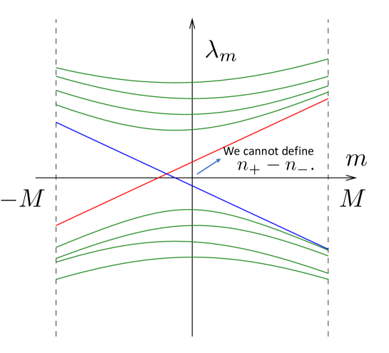
Figure 2: Example of the spectrum of $H(m)=\gamma_{5}(D+m)$ when $D$ does not respect the chiral symmetry. The massive definition or the number of crossings is still easy to count, while it is difficult to find a good definition of the chiral zero modes at $m=0$.

4 Atiyah-Patodi-Singer(APS) index (review)

So far, we have discussed fermions on a closed manifold without boundary. In this section, we consider a manifold with boundary and review the original Atiyah-Patodi-Singer index theorem and discuss why the formulation is physicist-unfriendly.

For simplicity, we consider a four-dimensional flat Euclidean compact manifold $X$ with a three-dimensional boundary $Y$. Let $D_{\rm APS}$ be a Dirac operator for the fermion field on $X$, to which the so-called APS boundary condition is imposed. Then the APS index theorem is

$${\rm Ind}D_{\rm APS}=\frac{1}{32\pi^{2}}\int_{X}d^{4}x\;\;\varepsilon^{\mu\nu\rho\sigma}{\rm tr}F_{\mu\nu}F_{\rho\sigma}(x)-\frac{1}{2}\eta(iD_{Y}),$$ (36)

where $iD_{Y}$ is a boundary Dirac operator on $Y$. As $Y$ is an odd-dimensional manifold, the eta invariant $\eta(iD_{Y})$ is a non-integer in general, which compensates the surface contribution of the first term to make the total RHS an integer.

This APS index theorem has not been that relevant in physics, since we were not interested in manifolds with boundary, which breaks the Lorentz invariance. However, recently, it attracts attention as pointed out in Ref.16 that the APS index is a key to understand the bulk-edge correspondence of topological insulators. In a topological insulator, the electrons in bulk is gapped, while the edge or surface modes become massless showing a good conductivity. The first term of Eq. (36) corresponds to the phase of bulk fermions, while the second term is that of edge modes. Each of them has anomaly in time-reversal $T$ symmetry, but the total contribution makes the theory $T$ invariant.

Let us look into the details. The massless edge mode’s determinant is

$$Z_{\rm edge} =\lim_{\mu\to\infty}\det\frac{D_{Y}}{D_{Y}+\mu}=\lim_{\mu\to\infty}\prod_{\lambda_{Y}}\frac{i\lambda_{Y}}{i\lambda_{Y}+\mu}\sim\lim_{\mu\to\infty}\prod_{\lambda_{Y}}\frac{i\lambda_{Y}}{\mu}$$

$$\propto\exp\left[-\frac{i\pi}{2}\sum_{\lambda_{Y}}{\rm sgn}(-\lambda_{Y})\right]=\exp\left[-\frac{i\pi}{2}\eta(iD_{Y})\right].$$ (37)

For the bulk massive fermions, from the results on a closed manifold we discussed in Eq. (3) setting $m=M$ and $\theta=\pi$ it is natural to assume that

$$Z_{\rm bulk} \propto\exp\left(i\pi\int_{X}d^{4}x\left[{\color[rgb]{0,0,0}\frac{1}{32\pi^{2}}\varepsilon^{\mu\nu\rho\sigma}{\rm tr}F_{\mu\nu}F_{\rho\sigma}(x)}\right]\right),$$ (38)

holds even when $X$ has a boundary. The total partition function is then

$$Z_{\rm bulk}Z_{\rm edge}\propto\exp(i\pi{\rm Ind}D_{\rm APS})=(-1)^{{\rm Ind}D_{\rm APS}},$$ (39)

which is $T$ invariant under the change of ${\rm Ind}D_{\rm APS}\to-{\rm Ind}D_{\rm APS}$.

In this way, the RHS of Eq. (36) has a natural interpretation in physics. But if you look at the definition of LHS, we would feel a bit uncomfortable.

Let us take our coordinate $x_{4}$ in the normal direction of the boundary $Y$ which is located at $x_{4}=0$. The Dirac operator near $x_{4}=0$ is written as

$$D_{\rm APS}=\gamma_{4}\left(\frac{\partial}{\partial x_{4}}+A\right),$$ (40)

where $A=\gamma_{4}\gamma_{i}D^{i}$ is the three-dimensional operator at $x_{4}=0$. The APS boundary condition requires the fermion fields to kill all the positive eigenmode components of $A$:

$$(A+|A|)\psi|_{x_{4}=0}=0,\;\;\;(A+|A|)D_{\rm APS}\psi|_{x_{4}=0}=0.$$ (41)

(For simplicity, we assume $A$ has no zero eigenvalue). This condition is nonlocal, as clear from a nonlocal operator $|A|$, and sensitive to the eigenfunctions of $A$, which is extended in $Y$.

The APS boundary condition keeps the anti-Hermiticity of $D_{\rm APS}$

$$0 =\int_{x_{4}>0}d^{4}x\phi_{2}^{\dagger}(x)D_{\rm APS}\phi_{1}(x)+\int_{x_{4}>0}d^{4}x(D_{\rm APS}\phi_{2})^{\dagger}(x)\phi_{1}(x)$$

$$=\int_{x_{4}=0}d^{3}x\phi_{2}^{\dagger}(x)\gamma_{4}\phi_{1}(x),$$ (42)

since $\{\gamma_{4},A\}=0$, and for any linear combination $\phi_{1}(x)$ of negative eigenmodes of $A$, $\gamma_{4}\phi_{1}(x)$ is that of positive eigenmodes. The condition also keeps the chirality $[\gamma_{5},A]=0$ well-defined, and with the anti-commutation relation $\{\gamma_{5},D_{\rm APS}\}$, the index can be written by the chiral zero modes, as usual: $n_{+}-n_{-}$.

In the standard Fujikawa method, let us perturbatively evaluate the index, with a heat kernel regulator,

$${\rm Ind}D_{\rm APS}=\lim_{s\to 0}{\rm Tr}\gamma_{5}e^{sD_{\rm APS}^{2}}.$$ (43)

Unlike on a closed manifold, the trace must be evaluated with a complete set satisfying the APS boundary condition. In the chiral representation,

$$A=\gamma_{4}\gamma_{i}D^{i}=\left(\begin{array}[]{cc}-i\sigma_{i}D^{i}&0\\ 0&i\sigma_{i}D^{i}\end{array}\right)=:\left(\begin{array}[]{cc}iD_{Y}&0\\ 0&-iD_{Y}\end{array}\right)=\tau_{3}\otimes iD_{Y}$$ (48)

and we can take a basis of the form below.

$$\phi_{\pm}^{\omega,\lambda}(x_{4})\otimes\phi_{\lambda}^{Y}(\bm{x})$$

where the subscript $\pm$ denotes the chirality: $\tau_{3}\phi_{\pm}^{\omega,\lambda}(x_{4})=\pm\phi_{\pm}^{\omega,\lambda}(x_{4})$, $\omega$ is the (absolute value of) momentum in the $x_{4}$ direction, and $\phi_{\lambda}^{Y}(\bm{x})$ is the eigenfunction of the surface Dirac operator $iD_{Y}$ (at $x_{4}=0$) with the eigenvalue $\lambda$: $iD_{Y}\phi_{\lambda}^{Y}(\bm{x})=\lambda\phi_{\lambda}^{Y}(\bm{x})$.

The APS boundary condition reads

$$\phi_{+}^{\omega,\lambda}(x_{4}=0) =0,\;\;\;\left.(\partial_{4}-\lambda)\phi_{-}^{\omega,\lambda}(x_{4})\right|_{x_{4}=0}=0,\;\;\;\mbox{for }\lambda>0,$$

$$\phi_{-}^{\omega,\lambda}(x_{4}=0) =0,\;\;\;\left.(\partial_{4}+\lambda)\phi_{+}^{\omega,\lambda}(x_{4})\right|_{x_{4}=0}=0,\;\;\;\mbox{for }\lambda<0,$$ (49)

to which the solutions are given by

$$\phi_{+}^{\omega,\lambda}(x_{4}) =\frac{e^{i\omega x_{4}}-e^{-i\omega x_{4}}}{\sqrt{2\pi}},\;\phi_{-}^{\omega,\lambda}(x_{4})=\frac{(i\omega+\lambda)e^{i\omega x_{4}}+(i\omega-\lambda)e^{-i\omega x_{4}}}{\sqrt{2\pi(\omega^{2}+\lambda^{2})}}\;\;\;\mbox{for }\lambda>0,$$

$$\phi_{-}^{\omega,\lambda}(x_{4}) =\frac{e^{i\omega x_{4}}-e^{-i\omega x_{4}}}{\sqrt{2\pi}},\;\phi_{+}^{\omega,\lambda}(x_{4})=\frac{(i\omega-\lambda)e^{i\omega x_{4}}+(i\omega+\lambda)e^{-i\omega x_{4}}}{\sqrt{2\pi(\omega^{2}+\lambda^{2})}}\;\;\;\mbox{for }\lambda<0,$$ (50)

where the eigenvalue of $D_{\rm APS}$ is $\pm i\sqrt{\lambda^{2}+\omega^{2}}$.

Interestingly, there is no edge-localized modes in the complete set. In fact, the Dirac equation $D_{\rm APS}\phi=\gamma_{4}(\partial_{4}+A)\phi=0$ has a formal solution $\exp(-\lambda x_{4})\otimes\phi_{\lambda}^{Y}(\bm{x})$ for any eigenvalue $\lambda$ of $A$, but the APS condition does not allow normalizable solutions with $\lambda>0$, which decays at $x_{4}=\infty$.

With the above complete set, we are now ready to compute the index perturbatively. At the leading order of the adiabatic expansion, ignoring the $x_{4}$ dependence of the gauge field, we have

$$\lim_{s\to 0}{\rm Tr}\gamma_{5}e^{sD_{\rm APS}^{2}}|_{LO} =\lim_{s\to 0}\sum_{\lambda}\int dx_{4}{\rm sgn}\lambda e^{-s\lambda^{2}}\int\frac{d\omega}{2\pi}\left(-1+\frac{2i|\lambda|}{\omega+i|\lambda|}e^{-s\omega^{2}+2i\omega x_{4}}\right)$$

$$=\lim_{s\to 0}\sum_{\lambda}{\rm sgn}\lambda\int_{0}^{\infty}dx_{4}\frac{\partial}{\partial x_{4}}\left[\frac{1}{2}e^{2|\lambda|x_{4}}{\rm erfc}(x_{4}\sqrt{s}+|\lambda|\sqrt{s})\right]$$

$$=-\frac{1}{2}\eta(iD_{Y}).$$ (51)

Here ${\rm erfc}(z)$ is the complementary error function,

$${\rm erfc}(x)=\frac{2}{\sqrt{\pi}}\int_{z}^{\infty}d\xi e^{-\xi^{2}},$$

which satisfies ${\rm erfc}(0)=1$ and ${\rm erfc}(\infty)=0$. From the next-to-leading order (NLO) contribution at bulk, we reproduce the curvature term,

$$\lim_{s\to 0}{\rm Tr}\gamma_{5}e^{sD_{\rm APS}^{2}}|_{NLO} =\frac{1}{32\pi^{2}}\int_{X}d^{4}x\;\;\varepsilon^{\mu\nu\rho\sigma}{\rm tr}F_{\mu\nu}F_{\rho\sigma}(x).$$ (52)

See Ref. 39 for the details. Thus we perturbatively confirmed the APS index theorem.

The APS condition has no problem in mathematics. To the first-order differential equations, we can put any boundary condition by hand. In physics, however, it is unnatural to keep helicity of one particle state as described in Sec. 1. Also, in quantum field theory, the quantum correction makes the boundary condition distorted, which could end up with a natural boundary condition in the continuum limit [41]. Specifically, the APS condition would receive a power divergent correction (expected from a naive dimensional analysis),

$$(A+|A|+c/a)\phi=0,$$ (53)

where $a$ is the short-range cut-off of the theory, which would end up with a Dirichlet condition in the continuum limit, unless we fine-tune the coefficient $c$, or require it to vanish imposing some symmetry. It is also clear that even if we could fine-tune $c$ to vanish, the system with the APS boundary condition, under which no edge localized mode can exist, is far different from topological insulators.

As a final discussion of this section, let us consider what is more physical setup. In physics, anything we regard as a boundary has “outside” of it. Topological insulators are nontrivial because their outside is covered by normal insulators (including air). Therefore, it would be better to consider physics with a domain-wall, separating two or more regions with different physical properties, rather than that on a manifold with a boundary. As discussed in this section, we should require angular momentum of particles to be preserved, rather than their helicity. The boundary condition should not be put by hand, but should be automatically chosen by nature. Hopefully the edge localized modes can exist and play a key role. In the next section, we will see that the domain-wall fermion perfectly matches these requirements.

5 APS index with domain-wall fermion

In this section, we show that the domain-wall Dirac operator can describe the APS index with different setup from the original one.

Let us recall Sec. 3, where we have confirmed that the AS index $I_{\rm AS}$ can be expressed by the massive Dirac operator, which is reflected in its determinant,

$$\det\left(\frac{D-M}{D+M}\right)\propto(-1)^{{\color[rgb]{0,0,0}I_{\rm AS}}}.$$ (54)

In this section, we consider a four-dimensional domain-wall fermion determinant,

$$\det\left(\frac{D-\varepsilon M}{D+M}\right),$$ (55)

where $\varepsilon$ denotes a position-dependent step function, for example, $\varepsilon={\rm sgn}(x_{4})$.

From the $\gamma_{5}$ Hermiticity: $\gamma_{5}D\gamma_{5}=-D=D^{\dagger}$, we find that the domain-wall fermion determinant is real, and we may assign an integer $I$

$$\det\left(\frac{D-\varepsilon M}{D+M}\right) =\det\left(\frac{\gamma_{5}(D-\varepsilon M)\gamma_{5}}{\gamma_{5}(D+M)\gamma_{5}}\right)=\det\left(\frac{D-\varepsilon M}{D+M}\right)^{*}\propto(-1)^{I},$$ (56)

to represent its sign. In the same way as in Sec. 3, we can express $I$ by the $\eta$ invariants as follows,

$$I=\frac{1}{2}\eta(H_{\rm DW})^{\rm PV.}=-\frac{1}{2}\eta(H_{\rm DW})+\frac{1}{2}\eta(H_{\rm PV}),$$ (57)

where $H_{\rm DW}=\gamma_{5}(D-\varepsilon M)$ and $H_{\rm PV}=\gamma_{5}(D+M)$. What is $I$ here? In fact, it is the APS index of $\varepsilon=+1$ region as will be shown below.

5.1 Perturbative evaluation of $\eta$ invariant of domain-wall Dirac operator

Let us perturbatively evaluate the $\eta$ invariant of the domain-wall Dirac operator,

$$\frac{1}{2}\eta(H_{DW}) =\frac{1}{2}{\rm Tr}\frac{H_{DW}}{\sqrt{H_{DW}^{2}}}={\rm Tr}\frac{H_{DW}}{\sqrt{\pi}}\int_{0}^{\infty}due^{-u^{2}H^{2}_{DW}}.$$ (58)

The short distance behavior around $u\sim 0$ for the large eigenvalues of $H_{DW}$, is again precisely canceled with that of the Pauli-Villars. In contrast to the AS index, the standard plane wave set does not work in evaluating the trace, since the translational symmetry is broken by the position-dependent mass term.

As an explicit example, we consider a flat four-dimensional torus of size $L^{3}\times 2T$, on which we put two domain-walls at $x_{4}=0$ and $x_{4}=T$. Taking the $A_{4}=0$ gauge, the domain-wall Dirac operator is given by

$$H_{\rm DW}=\gamma_{5}\left[\gamma_{i}D^{i}+\gamma_{4}\partial_{4}-M{\rm sgn}(x_{4}){\rm sgn}(T-x_{4})\right].$$ (59)

Near $x_{4}=0$ and taking the large $T$ limit, the solutions to

$$[H^{\rm free}_{\rm DW}]^{2}\phi=\left[-\partial_{\mu}^{2}+M^{2}+2M\gamma_{4}\delta(x_{4})\right]=\lambda^{2}\phi$$ (60)

are $\varphi^{\omega/{\rm edge}}_{\pm,e/o}(x_{4})\otimes e^{i\bm{p}\cdot\bm{x}}$, where the bulk modes

$$\varphi^{\omega}_{\pm,o}(x_{4}) =\frac{e^{i\omega x_{4}}-e^{-i\omega x_{4}}}{\sqrt{2\pi}},\varphi^{\omega}_{\pm,e}(x_{4})=\frac{(i\omega\pm M)e^{i\omega|x_{4}|}+(i\omega\mp M)e^{-i\omega|x_{4}|}}{\sqrt{2\pi(\omega^{2}+M^{2})}}$$ (61)

have eigenvalues $\lambda^{2}=\bm{p}^{2}+\omega^{2}+M^{2}$, and

$$\varphi^{\rm edge}_{-,e}(x_{4}) =\sqrt{M}e^{-M|x_{4}|},$$ (62)

are the chiral edge localized modes with $\lambda^{2}=\bm{p}^{2}$. Note here that the subscript $\pm$ indicates the eigenvalue of $\gamma_{4}$, and those with $e/o$ are even/odd under the reflection $x_{4}\to-x_{4}$. The edge modes appear only in the $\gamma_{4}=-1$ and even sector.

It is important to note that we did not put any boundary condition by hand. Nevertheless, they automatically satisfy

$$\left[\partial_{4}\mp M\varepsilon\right]\varphi^{\omega/{\rm edge}}_{\pm,e}(x_{4})|_{x_{4}=0}=0,\;\;\;\varphi^{\omega}_{\pm,o}(x_{4}=0)=0,$$ (63)

due to the domain-wall. More importantly, this condition is local and preserves angular-momentum in the $x_{4}$ direction, but does not keep the chirality.

For the edge modes, the domain-wall fermion Dirac operator acts as

$$H_{DW}\phi^{edge}(x) =\gamma_{5}(\gamma_{i}D^{i}+\underbrace{\gamma_{4}\partial_{4}-M\epsilon(x_{4})}_{=0})e^{i\bm{p}\cdot\bm{x}}P^{4}_{-}\varphi_{-,e}^{edge}(x_{4})$$

$$=(\gamma_{5}\gamma_{i}P^{4}_{-})D^{i}e^{i\bm{p}\cdot\bm{x}}\varphi_{-,e}^{edge}(x_{4})$$

$$=\left(\begin{array}[]{cc}0&0\\ 0&iD^{\rm 3D}\end{array}\right)e^{i\bm{p}\cdot\bm{x}}\varphi_{-,e}^{edge}(x_{4}),$$ (66)

where $P^{4}_{-}=\frac{1-\gamma_{4}}{2}$, $iD^{\rm 3D}=-i\sigma_{i}D^{i}(x_{4})$, and we have used notations

$$\gamma_{i} =\tau_{2}\otimes\sigma_{i},\;\gamma_{4}=\tau_{3}\otimes 1,\;\gamma_{5}=\tau_{1}\otimes 1,$$

$$\gamma_{5}\gamma_{i}P_{-}^{4} =(i\tau_{3}\otimes\sigma_{i})P_{-}^{4}=-\frac{1-\tau_{3}}{2}\otimes i\sigma_{i},$$ (67)

where $\sigma_{i}$ and $\tau_{i}$ are the Pauli matrices.

Then the edge mode’s contribution to the $\eta$ invariant is

$$-\frac{1}{2}\eta(H_{DW})^{edge}|_{x_{4}\sim 0} =-\frac{1}{2}\sum_{edgemodes}\phi^{edge}(x)^{\dagger}{\rm sgn}(H_{DW})\phi^{edge}(x)$$

$$=-\frac{1}{2}\sum_{edgemodes}\phi^{edge}(x)^{\dagger}\left[{\rm sgn}(iD^{\rm 3D}|_{x_{4}=0})+O(|x_{4}|)\right]\phi^{edge}(x)$$

$$=-\frac{1}{2}\eta(iD^{\rm 3D})|_{x_{4}=0}\times\left(\underbrace{\int dx_{4}(\varphi^{edge}_{-,e})^{\dagger}\varphi^{edge}_{-,e}(x_{4})}_{=1}+O(1/M)\right),$$ (68)

where we have used a fact that the $x_{4}$ dependence can be treated as an expansion with respect to $1/M$ for the edge modes,

$$\int_{-\infty}^{+\infty}dx_{4}[\varphi^{\rm edge}_{-,e}(x_{4})]^{\dagger}x_{4}^{n}\varphi^{\rm edge}_{-,e}(x_{4}) =M\int_{-\infty}^{+\infty}dx_{4}x_{4}^{n}e^{-2M|x_{4}|}$$

$$<M\int_{-\infty}^{+\infty}dx_{4}|x_{4}|^{n}e^{-2M|x_{4}|} =2M\int_{0}^{+\infty}dx_{4}x_{4}^{n}e^{-2Mx_{4}}$$

$$=2M(-1/2)^{n}\frac{\partial^{n}}{\partial M^{n}}\int_{0}^{+\infty}dx_{4}e^{-2Mx_{4}} =2M(-1/2)^{n}\frac{\partial^{n}}{\partial M^{n}}\left(\frac{1}{2M}\right)$$

$$=\left\{\begin{array}[]{cc}1&(n=0)\\ O(1/M^{n})&(n>0)\end{array}\right..$$ (71)

Adding contribution from another set of edge modes at $x_{4}=T$, we have

$$-\frac{1}{2}\eta(H_{DW})^{edge} =-\frac{1}{2}\eta(iD^{\rm 3D})|_{x_{4}=0}+\frac{1}{2}\eta(iD^{\rm 3D})|_{x_{4}=T},$$ (72)

up to $1/M$ corrections. The sign of the second term is positive, because the mass term changes the sign from negative to positive at $x_{4}=T$.

For the bulk modes, the eigenvalues satisfy $\lambda^{2}=\bm{p}^{2}+\omega^{2}+M^{2}>M^{2}$ and therefore, their contribution is local and it is easier to compute “density”,

$$-\frac{1}{2}\eta(H_{DW})^{bulk}{\color[rgb]{0,0,0}(x)} =-\frac{1}{2}\sum_{bulkmodes}\phi^{bulk}(x)^{\dagger}\frac{H_{DW}}{\sqrt{H_{DW}^{2}}}\phi^{bulk}(x)$$

$$=-\sum_{bulkmodes}\phi^{bulk}(x)^{\dagger}\frac{H_{DW}}{\sqrt{\pi}}\int_{0}^{\infty}due^{-u^{2}H^{2}_{DW}}\phi^{bulk}(x)$$

$$=-\left.\frac{1}{\sqrt{\pi}}\sum_{bulkmodes}\phi^{bulk}(x)^{\dagger}\right[$$

$$\left.({\color[rgb]{0,0,0}-\gamma_{5}M\epsilon(x_{4})}+\gamma_{5}D)\int_{0}^{\infty}due^{-u^{2}(\lambda^{2}+{\color[rgb]{0,0,0}\gamma_{[\mu,\nu]}F_{\mu\nu}})}\right]\phi^{bulk}(x)$$

$$=\frac{1}{64\pi^{2}}{\color[rgb]{0,0,0}\epsilon(x_{4})}\epsilon_{\mu\nu\rho\sigma}{\rm tr}_{c}F^{\mu\nu}F^{\rho\sigma}(x)+O(1/M).$$ (73)

See Ref. 11 for the details. An easier evaluation is to simply take the trace with the plane wave complete set. This should be valid as far as $x_{4}$ is larger than $1/M$, where the boundary effect is exponentially small. The Pauli-Villars contribution can be evaluated with the standard plane waves,

$$\frac{1}{2}\eta(H_{PV})^{bulk}(x) =\frac{1}{64\pi^{2}}\epsilon_{\mu\nu\rho\sigma}{\rm tr}_{c}F^{\mu\nu}F^{\rho\sigma}(x)+O(1/M).$$ (74)

Now the total index becomes

$$-\frac{1}{2}\eta(H_{\rm DW})+\frac{1}{2}\eta(H_{\rm PV}) =\frac{1}{32\pi^{2}}\int_{{\color[rgb]{0,0,0}0<x_{4}<T}}d^{4}x\epsilon_{\mu\nu\rho\sigma}{\rm tr}_{c}F^{\mu\nu}F^{\rho\sigma}(x)$$

$$-\frac{1}{2}\eta(iD^{\rm 3D})|_{x_{4}=0}+\frac{1}{2}\eta(iD^{\rm 3D})|_{x_{4}=T},$$ (75)

which coincides with the APS index on a cylinder $L^{3}\times[0,T]$. Here we have neglected $O(1/M)$ corrections. However, in Ref. 11, we have shown that the left-hand side of Eq. (5.1) is an $M$-independent integer, purely determined by the gauge field.

The boundary $\eta$ invariant represents the anomaly of time-reversal symmetry of the edge-localized mode of topological insulator, which is precisely canceled by that of the bulk modes. The bulk and edge decomposition of the domain-wall fermion Dirac operator matches this physical picture.

5.2 A non-perturbative proof

In the previous subsection, we have perturbatively confirmed the equality

$${\rm Ind}D_{\rm APS}=-\frac{1}{2}\eta(H_{\rm DW})^{\rm PV.}$$ (76)

on a flat four-dimensional manifold. The two quantities are defined on different manifolds. The original APS index is given on a manifold with boundary, while the $\eta$ invariant of the domain-wall Dirac operator is given on a closed manifold. The boundary conditions are also quite different. The readers may wonder if the equality is true on a general manifold or just a coincidence. In Ref. 12 we derived a theorem that for any APS index of a massless Dirac operator on a even-dimensional curved manifold $X_{+}$ with boundary, there exists a massive (domain-wall) Dirac operator on a closed manifold, sharing its half with $X_{+}$, and its $\eta$ invariant is equal to the original index. In this subsection, we give a physicist-friendly sketch of our mathematical proof.

First, we introduce a direct product $X\times\mathbb{R}$, where $X=X_{+}\cup X_{-}$ is a closed $2n$-dimensional manifold on which the domain-wall fermion lives. $X_{\pm}$ denotes the region where the mass term has $\pm$ sign. On this extended manifold, we modify the mass term as

$$m(x,s)=\left\{\begin{array}[]{cc}-M&\mbox{for $s>0$, $x\in X_{+}$}\\ +M&\mbox{otherwise}\end{array}\right.,$$ (79)

as presented in Fig. 3. Here $x$ denotes a coordinate in $X$ and $s$ is in the $\mathbb{R}$ direction. In this setup, we assume that the gauge field and metric on $X$ are just copied in the $s$ direction, and the $s$ component of the gauge field is zero. Note here that on the $s=+1$ slice, the mass term is the same as the original kink mass on $X$ and that on the $s=-1$ slice is positive everywhere in $X$ as in the Dirac operator on the Pauli-Villars field. Compared to the AS index case we discussed in Sec. 3.2, the domain-wall located at $s=0$ (or $x_{5}=0$) is bent and extended towards the $s=+\infty$ direction.

In a similar way as in Sec. 3.2, let us introduce a Dirac operator on a fermion field in $X\times\mathbb{R}$,

$$D_{\rm DW}^{2n+1}(M) =\tau_{2}\otimes\partial_{s}+i\tau_{1}\otimes\gamma_{5}(D+m(x,s))$$

$$=i\left(\begin{array}[]{cc}0&\partial_{s}+\gamma_{5}(D+m(x,s))\\ -\partial_{s}+\gamma_{5}(D+m(x,s))&0\end{array}\right).$$ (82)

We may call it a massless $2n+2$-dimensional Dirac operator, whose $2n+2$-th momentum is fixed to $m(x,s)$. In either interpretation, this Dirac operator $D_{\rm DW}^{2n+1}(M)$ has a chiral symmetry with $\gamma_{7}=\tau_{3}\otimes 1_{4\times 4}$.

Now let us solve the Dirac equation,

$$D_{\rm DW}^{2n+1}(M)\phi(x,s) =\left[\tau_{2}\otimes\partial_{s}+i\tau_{1}\otimes\gamma_{5}(D+m(x,s))\right]\phi(x,s)=0.$$ (83)

In the large $M$ limit, the zero mode solution must shrink around the domain-wall. For $x\in X_{+}$ and $s\sim 0$, they satisfy

$$\tau_{2}[1\otimes\partial_{s}-\tau_{3}\otimes\gamma_{5}M{\rm sgn}(s)]\phi(x,s)=0,$$ (84)

to which we find a edge-localized solution [8, 9] satisfying

$$\phi(x,s)\propto\exp(-M|s|),\;\;\;-\tau_{3}\otimes\gamma_{5}\phi(x,s)=+\phi(x,s)$$ (85)

and the massless Dirac equation $D\phi(x,s)=0$. Note that $\gamma_{7}=-\tau_{3}\otimes 1_{4\times 4}$ and $1_{2\times 2}\otimes\gamma_{5}$ must have the same eigenvalue.

For $x$ near the original domain-wall between $X_{+}$ and $X_{-}$, and $s>0$, the zero modes must satisfy

$$i\tau_{1}\otimes\gamma_{5}\gamma_{4}[\partial_{x_{4}}-\gamma_{4}M{\rm sgn}(x_{4})]\phi(x,s)=0,$$ (86)

where we denote the normal direction to the domain-wall by $x_{4}$, and the corresponding gamma matrix by $\gamma_{4}$. To this equation, we have edge-localized solution

$$\phi(x,s)\propto\exp(-M|x_{4}|),$$ (87)

which is chiral, $-1\otimes\gamma_{4}\phi(x,s)=+\phi(x,s)$. The zero modes also satisfy

$$\tau_{2}\otimes 1\left[1\otimes 1\partial_{s}+\tau_{3}\otimes\gamma_{5}(1\otimes\gamma_{i}D^{i})\right]\phi(x,s)$$

$$=\tau_{2}\otimes 1\left[1\otimes 1\partial_{s}-(1\otimes{\color[rgb]{0,0,0}\gamma_{4}}\gamma_{i}D^{i})(-\tau_{3}\otimes\gamma_{5})\right]\phi(x,s)=0.$$ (88)

Since $\gamma_{4}\gamma_{i}D^{i}$ is $s$-independent, it is natural to assume that the requirement $-\tau_{3}\otimes\gamma_{5}\phi(x,s=0)=\phi(x,s=0)$ at $s=0$ is inherited to the all range of $s>0$.

Here let us define $A=\gamma_{4}\gamma_{i}D^{i}$ and its eigenvalues and states by $\lambda_{A}$ and $\phi_{\lambda_{A}}(\bm{x})$, respectively. The above Dirac equation is now simplified as

$$(\partial_{s}-A)\phi(x)=0,$$ (89)

and the solution is given by a linear combination of $\phi_{\lambda_{A}}(\bm{x})$,

$$\phi(x)=\sum_{\lambda_{A}}\alpha_{\lambda_{A}}\phi_{\lambda_{A}}(\bm{x})\exp(\lambda_{A}s).$$ (90)

Note that the coefficient $\alpha_{\lambda_{A}}$ must be zero for $\lambda_{A}>0$, otherwise, the solution is not normalizable. Interestingly, this constraint is exactly the same as the APS boundary condition at the boundary of $X_{+}$ and $s=0$.

This is not a coincidence but proved in the original APS paper[3, 4, 5]: the APS index is equal to the index on a manifold with an infinite cylinder attached to the original boundary, with respect to the square integrable modes. Here, the gauge field and metric are just copied along the cylinder.

To summarize, the solution to $D_{\rm DW}^{2n+1}(M)\phi(x,s)=0$ with chirality $\gamma_{7}=\pm 1$ must satisfy $D\phi(x,s=0)=0$ with the same chirality of $\gamma_{5}$ in the region $x\in X_{+}$ and satisfy the APS boundary condition at the boundary. Namely, we have shown that ${\rm Ind}(D_{\rm DW}^{2n+1}(M))={\rm Ind}_{\rm APS}(D|_{X_{+}})$.

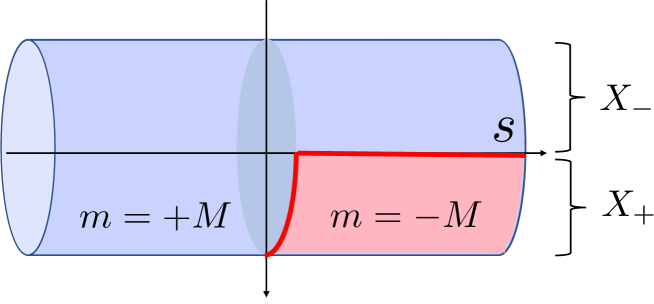
Figure 3: The cylindrical manifold $X\times\mathbb{R}$ and the mass configuration.

Next we consider the same Dirac equation but at $s=\pm\infty$. At $s=-\infty$, the equation is

$$0 =\left[\tau_{2}\otimes\partial_{x_{5}}+i\tau_{1}\otimes\gamma_{5}(D+M)\right]\phi(x)=\tau_{2}\left[1\otimes\partial_{x_{5}}+\tau_{3}\otimes H_{\rm PV}\right]\phi(x).$$ (91)

For $\gamma_{7}=\tau_{3}=\pm 1$, the solution is a linear combination of

$$\exp(\mp\lambda_{\rm PV}s),$$

where $\lambda_{\rm PV}$ is an eigenvalue of $H_{\rm PV}$, which is normalizable only when ${\rm sgn}(\lambda_{\rm PV})=\mp 1$, in the $s\to-\infty$ limit. At $s=+\infty$, the domain-wall fermion Dirac operator appears,

$$0 =\left[\tau_{2}\otimes\partial_{x_{5}}+i\tau_{1}\otimes\gamma_{5}(D-\varepsilon M)\right]\phi(x)=\tau_{2}\left[1\otimes\partial_{x_{5}}+\tau_{3}\otimes H_{\rm DW}\right]\phi(x),$$ (92)

where $\varepsilon(x)=+1$ for $x\in X_{+}$ and -1, otherwise. For $\gamma_{7}=\tau_{3}=\pm 1$, the solution is a linear combination of

$$\exp(\mp\lambda_{\rm DW}s),$$

where $\lambda_{\rm DW}$ is an eigenvalue of $H_{\rm DW}$, which is normalizable only when ${\rm sgn}(\lambda_{\rm DW})=\pm 1$, in the $s\to\infty$ limit.

Now the proof goes the exactly same way as in the AS index shown in Sec. 3.2. Smoothing the step function and considering an adiabatic $s$ dependence of the solutions, we can assign a one-to-one correspondence between the solution and the one-parameter family of each eigenvalue $\lambda_{s}$ of the Hermitian Dirac operator on the slice $s$. For a $\gamma_{7}=+1$ zero mode, we have to find a $\lambda_{s}$ with $\lambda_{\rm PV}<0$ (at $s=-\infty$) and $\lambda_{\rm DW}>0$ (at $s=+\infty$), while for $\gamma_{7}=-1$ we have to find the one with $\lambda_{\rm PV}>0$ and $\lambda_{\rm DW}<0$. The index is given by the spectral flow along the path $s\in[-\infty,+\infty]$ counting the increased number of the positive eigenvalues subtracted by that of the negative eigenvalues divided by 2:

$${\rm Ind}[D_{\rm DW}^{2n+1}(M)] =\frac{1}{2}\sum_{\lambda_{\rm PV}}{\rm sgn}(\lambda_{\rm PV})-\frac{1}{2}\sum_{\lambda_{\rm DW}}{\rm sgn}(\lambda_{\rm DW}),$$ (93)

which is equal to the RHS of Eq. (76). The proof for our main theorem is complete.

In this section, have perturbatively and non-perturbatively shown that

$$\left({\rm Ind}(D_{\rm DW}^{2n+1}(M))=\right){\rm Ind}_{\rm APS}(D|_{X_{+}})=-\frac{1}{2}\eta(H_{\rm DW})+\frac{1}{2}\eta(H_{\rm PV}).$$ (94)

For the massive expression, the chiral symmetry is not crucial at all and we do not need any nonlocal boundary conditions. In the next section, we will see that this massive formulation is valid even on a lattice.

6 APS index on a lattice

After a long history of chiral symmetry in lattice gauge theory since Refs. 44, 45, it is now well-known that the Atiyah-Singer index on an even-dimensional torus can be formulated even with finite lattice spacings[46]. This is possible using the overlap Dirac operator[47] or that in the perfect action[48], satisfying the Ginsparg-Wilson relation[49], as a consequence of the exactness of the modified lattice chiral symmetry[50]. However, its extension to the APS index has been untouched due to the difficulty of the nonlocal boundary condition. In this section, we show that the domain-wall Dirac operator can formulate the APS index even on a lattice[13].

The difficulty of the chiral symmetry originates from the periodic boundary condition of the momentum space in lattice gauge theory. The naive Dirac operator $i\gamma^{\mu}p_{\mu}$ is replaced by $i\gamma^{\mu}\sin(p_{\mu}a)/a$ with a lattice spacing $a$, which has 15 unphysical poles, as $p_{\mu}$ for each direction $\mu$ has two zero points $p_{\mu}=0$ and $p_{\mu}=\pi/a$. To remove the unwanted modes called doublers, one needs to add a momentum-dependent mass term (Wilson term), which explicitly breaks the chiral symmetry. Since the Nielsen-Ninomiya theorem[44, 45] proved that the chiral symmetry must be broken in order to remove the doublers, it has been a challenge to formulate an exactly chiral symmetric fermion on a lattice.

In fact, there is one symmetry which must be explicitly broken on a lattice. It is the axial $U(1)$ symmetry. If there is a lattice Dirac operator free from doublers which breaks the axial $U(1)$ only, we are able to respect all other part of chiral symmetries $SU(N_{f})_{L}\times SU(N_{f})_{R}\times U(1)_{V}$, where $N_{f}$ is the number of flavors, in a lattice gauge theory.

The overlap Dirac operator[47] perfectly meets the desired conditions. It is defined by

$$D_{ov}=\frac{1}{a}\left(1+\gamma_{5}\frac{H_{W}}{\sqrt{H_{W}^{2}}}\right),$$ (95)

where $H_{W}=\gamma_{5}(D_{W}-M)$ is a massive Wilson Dirac operator with a cut-off scale mass $M=1/a$, and satisfies the Ginsparg-Wilson relation

$$\gamma_{5}D_{ov}+D_{ov}\gamma_{5}=aD_{ov}\gamma_{5}D_{ov}.$$ (96)

The overlap fermion action $S=\sum_{x}\bar{\psi}D_{ov}\psi(x)$ is invariant under the modified chiral transformation,

$$\psi\to e^{i\alpha\gamma_{5}(1-aD_{ov})}\psi,\;\;\;\bar{\psi}\to\bar{\psi}e^{i\alpha\gamma_{5}},$$ (97)

but the fermion measure transforms as

$$d\psi d\bar{\psi}\to\exp\left[i\alpha{\rm Tr}(\gamma_{5}+\gamma_{5}(1-aD_{ov}))\right]d\psi d\bar{\psi},$$ (98)

which precisely reproduces the axial $U(1)$ anomaly. Moreover,

$${\rm Tr}\gamma_{5}\left(1-\frac{aD_{ov}}{2}\right),$$ (99)

corresponds to the Atiyah-Singer index. It is known that the eigenvalue spectrum of the overlap Dirac operator makes a circle of radius $1/a$ whose center is located at $1/a$ in the complex plane. We can show that the complex eigenvalues of $D_{\rm ov}$ make $\pm$ pairs of the “chirality” operator $\gamma_{5}\left(1-\frac{aD}{2}\right)$ and the real modes at $2/a$, which corresponds to the doublers, do not contribute. Thus the above trace essentially counts the index of $D_{ov}$.

Despite a remarkable success of the AS index in lattice gauge theory, its extension to the APS has been not known. In continuum theory, the Dirac operator can be decomposed as $D=\gamma^{4}D_{4}+\gamma^{i}D_{i}$, and the APS boundary condition is imposed with respect to the eigenfunctions of $\gamma_{4}\gamma^{i}D_{i}$, which corresponds to the Dirac operator on the boundary. For the lattice Dirac operator $D_{ov}$, there is no simple way to separate the boundary part of the operator. Moreover, it was shown in Ref. 41 that any boundary condition but periodic or anti-periodic boundary conditions breaks the Ginsparg-Wilson relation.

Although formulating the APS index of a massless lattice Dirac operator looks hopeless, a great hint is hidden in the formulation of the AS index. Simply substituting the definition of the overlap Dirac operator into Eq. (99), we end up with the $\eta$ invariant of the massive Wilson Dirac operator,

$${\rm Ind}(D_{ov})=-\frac{1}{2}{\rm Tr}\frac{H_{W}}{\sqrt{H_{W}^{2}}}=-\frac{1}{2}\eta(\gamma_{5}(D_{W}-M)).$$ (100)

Surprisingly, the lattice AS index theorem “knew” that the index can be given with massive Dirac operator and chiral symmetry is not important: the Wilson Dirac operator is enough to define it.

Let us here summarize the situation in Tab. 6 and 6. The standard index theorems with respect to the massless fermion Dirac operator requires much efforts to formulate. The APS index elaborates a nonlocal (and unphysical) boundary condition, the lattice AS needs a complicated chiral Dirac operator satisfying the Ginsparg-Wilson relation, and the lattice version of APS is not even known yet. Instead, the $\eta$ invariant of the massive Dirac operator offers a unified description of the index theorems on a closed manifold. The APS index is obtained by just changing the sign of the mass on a domain-wall. The lattice version of the AS index is given by the Wilson Dirac operator, even without knowing its equivalence to the index of the overlap Dirac operator. As already shown in Fig. 2, the massive bulk definition is stable against symmetry breaking of the original Dirac operator, as it counts one-dimensional objects, the spectral flow, rather than points of the massless Dirac operator spectrum. It is now natural to speculate that the lattice formulation of the APS index is given by the $\eta$ invariant of lattice domain-wall Dirac operator

$$-\frac{1}{2}\eta(\gamma_{5}(D_{W}-\varepsilon M)).$$ (101)

In Ref. 13, by a tedious but straight-forward perturbative computation, we have shown on a four-dimensional Euclidean lattice with periodic boundary conditions (of which continuum limit is $T^{4}$) that

$$-\frac{1}{2}\eta(\gamma_{5}(D_{W}-\varepsilon M_{1}+M_{2}))= \frac{1}{32\pi^{2}}\int_{{\color[rgb]{0,0,0}0<x_{4}<T}}d^{4}x\epsilon_{\mu\nu\rho\sigma}{\rm tr}_{c}F^{\mu\nu}F^{\rho\sigma}(x)$$

$$+\frac{1}{2}\eta(iD^{\rm 3D})|_{x_{4}=0}-\frac{1}{2}\eta(iD^{\rm 3D})|_{x_{4}=T}+O(a),$$ (102)

where $\varepsilon={\rm sgn}(x_{4}-a/2){\rm sgn}(T-x_{4}-a/2)$ represent two domain-walls we put at $x_{4}=a/2$ and $x_{4}=T-a/2$ with the lattice spacing $a$. The LHS is shown in the limit $M_{1}+M_{2}\to\infty$ while $M=M_{1}-M_{2}$ is fixed. Note that the left-hand side is always an integer. Therefore, we expect that this definition of the APS index on the lattice is nonperturbatively valid, with possibly additional requirement on the smoothness of the gauge link variables[56].

The standard formulation with massless Dirac operator continuum lattice AS ${\rm Tr}\gamma_{5}e^{D^{2}/M^{2}}$ ${\rm Tr}\gamma_{5}(1-aD_{ov}/2)$ APS ${\rm Tr}\gamma_{5}e^{D^{2}/M^{2}}$ w/ APS b.c. not known.

The $\eta$ invariant of massive Dirac operator continuum lattice AS $-\frac{1}{2}\eta(\gamma_{5}(D-M))^{\rm PV.}$ $-\frac{1}{2}\eta(\gamma_{5}(D_{W}-M))$ APS $-\frac{1}{2}\eta(\gamma_{5}(D-\varepsilon M))^{\rm PV.}$ $-\frac{1}{2}\eta(\gamma_{5}(D_{W}-\varepsilon M))$

7 Mod-two APS index

So far we have only considered the standard index taking an integer value on an even-dimensional manifold. In Ref. 15, we extended our work to the odd-dimensional cases, which have the so-called mod-two index defined by the number of zero modes mod 2. The mod-two index makes sense only when the Dirac operator is real where every nonzero mode makes a $\pm$ pair: for $D\phi=i\lambda\phi$, we have $D\phi^{*}=-i\lambda\phi^{*}$. If one non-zero mode goes down to zero, so does its pair with the opposite sign. The number of zero modes can change by even numbers only under smooth variation of the gauge field and metric.

In the odd-dimensional case, we cannot use the $\eta$ invariant. Instead, we have the so-called spectral flow. As we have seen in Sec. 5, the $\eta$ invariant is also equivalent to the spectral flow:

$${\rm Sf}[H_{1}]_{H_{0}}=-\frac{1}{2}\eta(H_{1})+\frac{1}{2}\eta(H_{0}),$$ (109)

where the two Hermitian operator $H_{0}$ and $H_{1}$ are smoothly connected by a one-parameter family $H_{t}$.

For a real Dirac operator $D$ (in odd dimensions), we introduce a doubled spinor field and an anti-Hermitian and real massive Dirac operator on it,

$$A(m):=\left(\begin{array}[]{cc}&D+m\\ -(D+m)^{\dagger}&\end{array}\right).$$ (112)

and using the mod-two spectral flow[57, 58], ${\rm Sf}_{\rm 2}[A_{1}]_{A_{0}}$, which is defined by the number of zero-crossing pairs along the one-parameter family $A_{t}$ $t\in[0,1]$, we have proved that

$${\rm Sf}_{\rm 2}[A(-\varepsilon M)]_{A(M)},$$ (113)

is equal to the mod-two APS index ${\rm Ind}^{\rm mod-2}_{\rm APS}(D)$ in the $\varepsilon=+1$ region.

Moreover, we showed that the index is related to the domain-wall fermion determinant by

$$\det\frac{D-\varepsilon M}{D+M}\propto(-1)^{{\rm Ind}^{\rm mod-2}_{\rm APS}(D)},$$ (114)

which allows us to decompose the edge and bulk contributions as

$${\rm Ind}_{\rm APS}(D) = I_{\rm edge}+I_{\rm bulk}\;\;\;(\mbox{mod 2}),$$

$$I_{\rm edge} = \frac{1-{\rm sgn}\left[\det D_{\rm edge}\right]}{2},$$

$$I_{\rm bulk} = \frac{1-{\rm sgn}\left[\det D_{\rm bulk}\right]}{2}.$$ (115)

Here,

$$D_{\rm edge} :=\left(\begin{array}[]{cc}D-\varepsilon M&0\\ 0&\partial+\varepsilon M\end{array}\right)\left(\begin{array}[]{cc}D-\varepsilon M&\mu I\\ \mu I^{-1}&\partial+\varepsilon M\end{array}\right)^{-1},$$ (120)

$$D_{\rm bulk} :=\left(\begin{array}[]{cc}D-\varepsilon M&\mu I\\ \mu I^{-1}&\partial+\varepsilon M\end{array}\right)\left(\begin{array}[]{cc}D+M&0\\ 0&\partial+M\end{array}\right)^{-1},$$ (125)

where $\partial$ denotes the free Dirac operator and the mass $\mu\ll M$, which breaks the gauge symmetry, is introduced to give an ultra-violet cut-off to the edge modes, while it is the infra-red cut-off for the bulk modes. Since $D_{\rm edge}$ and $D_{\rm bulk}$ are both real, the decomposition represents the inflow of the global anomaly[59, 60, 61, 62].

Note that the lattice Wilson Dirac operator inherits the real structure of the operator, and the lattice version of $A(m)$,

$$A_{W}(m):=\left(\begin{array}[]{cc}&D_{W}+m\\ -(D_{W}+m)^{\dagger}&\end{array}\right)$$ (128)

and the corresponding mod-two spectral flow from the spectrum of a reference operator $A_{W}(M)$ can be defined without any difficulty. Therefore, as shown in Tab. 7, this achieves a further unification of the index theorems: the standard/mod-two AS/APS index in continuum/lattice theory can be reformulated by the spectral flow of a massive Dirac operator on a closed manifold without boundary.

The spectral flow of massive Dirac operator continuum lattice AS ${\rm Sf}[\gamma_{5}(D-M)]_{H(M)}$ ${\rm Sf}[\gamma_{5}(D_{W}-M)]_{H_{W}(M)}$ APS ${\rm Sf}[\gamma_{5}(D-\varepsilon M)]_{H(M)}$ ${\rm Sf}(\gamma_{5}(D_{W}-\varepsilon M)]_{H_{W}(M)}$ mod-2 AS ${\rm Sf}_{2}\left[\left(\begin{array}[]{cc}&D-M\\ -(D-M)^{\dagger}&\end{array}\right)\right]_{A(M)}$ ${\rm Sf}_{2}\left[\left(\begin{array}[]{cc}&D_{W}-M\\ -(D_{W}-M)^{\dagger}&\end{array}\right)\right]_{A_{W}(M)}$ mod-2 APS ${\rm Sf}_{2}\left[\left(\begin{array}[]{cc}&D-\varepsilon M\\ -(D-\varepsilon M)^{\dagger}&\end{array}\right)\right]_{A(M)}$ ${\rm Sf}_{2}\left[\left(\begin{array}[]{cc}&D_{W}-\varepsilon M\\ -(D_{W}-\varepsilon M)^{\dagger}&\end{array}\right)\right]_{A_{W}(M)}$

8 Summary and discussion

In this review, we have shown that the axial anomaly and index theorems can be understood with massive fermions. The $\eta$ invariant or spectral flow of the massive Dirac operator, including the domain-wall Dirac operator, on a closed manifold without boundary, gives a unified view of different types of index theorems. The formulation is physicist-friendly enough that the application to lattice gauge theory is straightforward.

The massive formulation of the index theorems have a tight connection to physics of topological insulators. The edge-localized modes appear at the domain-wall, and describe the $\eta$ invariant of the boundary operator. Unlike the original formulation of APS, the non-locality of the $\eta$ invariant is not a consequence of the boundary condition, but reflects the massless nature of the edge modes. From the bulk mode contribution, which is massive, we obtain a local expression of the curvature term.

In order to identify the topological and normal phases of massive fermions, it is essential to choose a regularization of the $\eta$ invariant that distinguishes the sign of the mass. In this paper, we have chosen the Pauli-Villars subtraction in continuum theory, and Wilson Dirac operator on a lattice. We have set the coefficients of the Pauli-Villars mass and the Wilson term positive, and the domain of the topological phase is identified as that having negative fermion mass. It may be difficult to formulate the anomaly (inflow) with regularizations which cannot distinguish the sign of the mass, such as dimensional or heat kernel regularizations.

The equivalence of the massive formulation to the original AS or APS has been proven through the index of a higher-dimensional Dirac operator $D_{\rm DW}^{2n+1}(M)$ on $X\times\mathbb{R}$. Since the extended manifold has cylindrical ends at $s\to\pm\infty$, the index is equal to the index on $X\times[-1,1]$, where the APS boundary condition is imposed at $s=\pm 1$. Then an interesting question is if we can express this higher-dimensional index by the $\eta$ invariant again:

$${\rm Ind}_{\rm APS}(D_{\rm DW}^{2n+1}(M)|_{X\times[-1,1]})=-\frac{1}{2}\eta(\gamma_{7}(D_{\rm DW}^{2n+1}(M)-\mu\kappa))^{\rm PV.},$$ (142)

where we have introduced a second mass term $\mu\kappa$ with $\kappa=1$ in $s\in[-1,1]$, and $-1$, otherwise. In this “doubly” domain-wall fermion, the original edge mode localized in $2n-1$ dimensional manifold $Y$ becomes the edge-of-edge states[63, 64, 65] of $\gamma_{7}(D_{\rm DW}^{2n+1}(M)-\mu\kappa)$, which is localized at the junction of the first and second domain-walls. This recursive structure might be useful for understanding physics of higher order topological insulators[66, 67].

Our work is limited to the real and pseudo-real fermions. In the literature[68, 69, 42], it is claimed that the phase of the massive complex fermion is controlled by the $\eta$ invariant of a massless Dirac operator with the APS boundary condition. It would be interesting to study if the domain-wall fermion can reformulate the phase of the complex fermion determinant without any nonlocal boundary conditions.

As a final discussion, let us reconsider the difference between massless and massive systems. In physics, we have been imprinted that a symmetry makes some particle fields massless, which leads to a good control of understanding nature. For example, the gauge symmetry in the Yang-Mills fields makes gauge bosons massless, which guarantees that the theory renormalizable. Even when the symmetry is broken, if it is spontaneous, we still have a good control of the theory, thanks to the Nambu-Goldstone theorem[70, 71]. Such a “symmetry fundamentalism” that massless is better than massive, has been a driving force in particle physics and successful for 50 years. However, we have also experienced problems where we cannot find any relevant symmetry to explain the small scales of the particles, such as the Higgs boson mass. In this review, we have seen that massive fermion is not always inferior to the massless chiral fermion, but sometimes gives mathematically equal or better understanding of physics. In the systems we used in this article, the symmetry appears not as a guiding principle of the theory but as an accidental consequence of the localization of edge modes in the massive system. It would be nice if our works could give a hint for the “post-symmetry” era of new physics.

References

- [1] M. F. Atiyah and I. M. Singer, “The index of elliptic operators on compact manifolds,” Bull. Am. Math. Soc. 69, 422 (1963). doi:10.1090/S0002-9904-1963-10957-X
- [2] M. F. Atiyah and I. M. Singer, “The Index of elliptic operators. 1,” Annals Math. 87, 484 (1968). doi:10.2307/1970715
- [3] M. F. Atiyah, V. K. Patodi and I. M. Singer, “Spectral asymmetry and Riemannian Geometry I,” Math. Proc. Cambridge Phil. Soc. 77, 43 (1975). doi:10.1017/S0305004100049410
- [4] M. F. Atiyah, V. K. Patodi and I. M. Singer, “Spectral asymmetry and Riemannian geometry II,” Math. Proc. Cambridge Phil. Soc. 78, 405 (1975). doi:10.1017/S0305004100051872
- [5] M. F. Atiyah, V. K. Patodi and I. M. Singer, “Spectral asymmetry and Riemannian geometry. III,” Math. Proc. Cambridge Phil. Soc. 79, 71 (1976). doi:10.1017/S0305004100052105
- [6] S. L. Adler, “Axial vector vertex in spinor electrodynamics,” Phys. Rev. 177, 2426-2438 (1969) doi:10.1103/PhysRev.177.2426
- [7] J. Bell and R. Jackiw, “A PCAC puzzle: in the model,” Nuovo Cim. A 60, 47-61 (1969) doi:10.1007/BF02823296
- [8] R. Jackiw and C. Rebbi, “Solitons with Fermion Number 1/2,” Phys. Rev. D 13, 3398-3409 (1976) doi:10.1103/PhysRevD.13.3398
- [9] C. G. Callan, Jr. and J. A. Harvey, “Anomalies and Fermion Zero Modes on Strings and Domain Walls,” Nucl. Phys. B 250, 427-436 (1985) doi:10.1016/0550-3213(85)90489-4
- [10] D. B. Kaplan, “A Method for simulating chiral fermions on the lattice,” Phys. Lett. B 288, 342 (1992) doi:10.1016/0370-2693(92)91112-M [hep-lat/9206013].
- [11] H. Fukaya, T. Onogi and S. Yamaguchi, “Atiyah-Patodi-Singer index from the domain-wall fermion Dirac operator,” Phys. Rev. D 96, no.12, 125004 (2017) doi:10.1103/PhysRevD.96.125004 [arXiv:1710.03379 [hep-th]]; “Atiyah-Patodi-Singer index theorem for domain-wall fermion Dirac operator,” EPJ Web Conf. 175, 11009 (2018) doi:10.1051/epjconf/201817511009 [arXiv:1712.03679 [hep-lat]].
- [12] H. Fukaya, M. Furuta, S. Matsuo, T. Onogi, S. Yamaguchi and M. Yamashita, “The Atiyah-Patodi-Singer index and domain-wall fermion Dirac operators,” Commun. Math. Phys. 380, no.3, 1295-1311 doi:10.1007/s00220-020-03806-0 [arXiv:1910.01987 [math.DG]].
- [13] H. Fukaya, N. Kawai, Y. Matsuki, M. Mori, K. Nakayama, T. Onogi and S. Yamaguchi, “Atiyah-Patodi-Singer index on a lattice,” PTEP 2020, no.4, 043B04 (2020) doi:10.1093/ptep/ptaa031 [arXiv:1910.09675 [hep-lat]].
- [14] T. Onogi and T. Yoda, “Comments on the Atiyah-Patodi-Singer index theorem, domain wall, and Berry phase,” JHEP 12, 096 (2021) doi:10.1007/JHEP12(2021)096 [arXiv:2109.08274 [hep-th]].
- [15] H. Fukaya, M. Furuta, Y. Matsuki, S. Matsuo, T. Onogi, S. Yamaguchi and M. Yamashita, “Mod-two APS index and domain-wall fermion,” [arXiv:2012.03543 [hep-th]].
- [16] E. Witten, “Fermion Path Integrals And Topological Phases,” Rev. Mod. Phys. 88, no.3, 035001 (2016) doi:10.1103/RevModPhys.88.035001 [arXiv:1508.04715 [cond-mat.mes-hall]].
- [17] G. ’t Hooft, “Naturalness, chiral symmetry, and spontaneous chiral symmetry breaking,” NATO Sci. Ser. B 59, 135-157 (1980)
- [18] Y. Hatsugai, “Chern number and edge states in the integer quantum Hall effect,” Phys. Rev. Lett. 71, no. 22, 3697 (1993). doi:10.1103/PhysRevLett.71.3697; “Edge states in the integer quantum Hall effect and the Riemann surface of the Bloch function,” Phys. Rev. B 48, no. 16, 11851 (1993). doi:10.1103/PhysRevB.48.11851
- [19] M. Kurkov and D. Vassilevich, “Gravitational parity anomaly with and without boundaries,” JHEP 03, 072 (2018) doi:10.1007/JHEP03(2018)072 [arXiv:1801.02049 [hep-th]].
- [20] Y. Tachikawa and K. Yonekura, “Why are fractional charges of orientifolds compatible with Dirac quantization?,” SciPost Phys. 7, no.5, 058 (2019) doi:10.21468/SciPostPhys.7.5.058 [arXiv:1805.02772 [hep-th]].
- [21] D. Vassilevich, “Index Theorems and Domain Walls,” JHEP 07, 108 (2018) doi:10.1007/JHEP07(2018)108 [arXiv:1805.09974 [hep-th]].
- [22] I. García-Etxebarria and M. Montero, “Dai-Freed anomalies in particle physics,” JHEP 08, 003 (2019) doi:10.1007/JHEP08(2019)003 [arXiv:1808.00009 [hep-th]].
- [23] K. Yonekura, “Anomaly matching in QCD thermal phase transition,” JHEP 05, 062 (2019) doi:10.1007/JHEP05(2019)062 [arXiv:1901.08188 [hep-th]].
- [24] C. T. Hsieh, Y. Tachikawa and K. Yonekura, “Anomaly inflow and -form gauge theories,” [arXiv:2003.11550 [hep-th]].
- [25] Y. Hamada, J. M. Pawlowski and M. Yamada, “Gravitational instantons and anomalous chiral symmetry breaking,” [arXiv:2009.08728 [hep-th]].
- [26] A. Gromov, K. Jensen and A. G. Abanov, “Boundary effective action for quantum Hall states,” Phys. Rev. Lett. 116, no. 12, 126802 (2016) doi:10.1103/PhysRevLett.116.126802 [arXiv:1506.07171 [cond-mat.str-el]].
- [27] M. A. Metlitski, “-duality of gauge theory with on non-orientable manifolds: Applications to topological insulators and superconductors,” arXiv:1510.05663 [hep-th].
- [28] N. Seiberg and E. Witten, “Gapped Boundary Phases of Topological Insulators via Weak Coupling,” PTEP 2016, no.12, 12C101 (2016) doi:10.1093/ptep/ptw083 [arXiv:1602.04251 [cond-mat.str-el]].
- [29] Y. Tachikawa and K. Yonekura, “Gauge interactions and topological phases of matter,” PTEP 2016, no. 9, 093B07 (2016) doi:10.1093/ptep/ptw131 [arXiv:1604.06184 [hep-th]].
- [30] D. S. Freed and M. J. Hopkins, “Reflection positivity and invertible topological phases,” arXiv:1604.06527 [hep-th].
- [31] Y. Yu, Y. S. Wu and X. Xie, “Bulk-edge correspondence, spectral flow and Atiyah-Patodi-Singer theorem for the Z2 -invariant in topological insulators,” Nucl. Phys. B 916, 550 (2017) doi:10.1016/j.nuclphysb.2017.01.018 [arXiv:1607.02345 [cond-mat.mes-hall]].
- [32] K. Hasebe, “Higher (Odd) Dimensional Quantum Hall Effect and Extended Dimensional Hierarchy,” Nucl. Phys. B 920, 475 (2017) doi:10.1016/j.nuclphysb.2017.03.017 [arXiv:1612.05853 [hep-th]].
- [33] K. Yonekura, “On the cobordism classification of symmetry protected topological phases,” Commun. Math. Phys. 368, no.3, 1121-1173 (2019) doi:10.1007/s00220-019-03439-y [arXiv:1803.10796 [hep-th]].
- [34] Y. Yao and M. Oshikawa, “Generalized Boundary Condition Applied to Lieb-Schultz-Mattis-Type Ingappabilities and Many-Body Chern Numbers,” Phys. Rev. X 10, no.3, 031008 (2020) doi:10.1103/PhysRevX.10.031008 [arXiv:1906.11662 [cond-mat.str-el]].
- [35] K. Fujikawa and H. Suzuki, “Path integrals and quantum anomalies,” Oxford : Clarendon Press, 2004, doi:10.1093/acprof:oso/9780198529132.001.0001
- [36] S. Aoki et al. [Flavour Lattice Averaging Group], “FLAG Review 2019: Flavour Lattice Averaging Group (FLAG),” Eur. Phys. J. C 80, no.2, 113 (2020) doi:10.1140/epjc/s10052-019-7354-7 [arXiv:1902.08191 [hep-lat]].
- [37] E. Witten, “Supersymmetry and Morse theory,” J. Diff. Geom. 17, no.4, 661-692 (1982)
- [38] Furuta, M.: Index theorem. 1, Translations of Mathematical Monographs, 235, Translated from the 1999 Japanese original by Kaoru Ono; Iwanami Series in Modern Mathematics, American Mathematical Society, Providence, RI, xviii+205, MR2361481 (2007)
- [39] L. Alvarez-Gaume, S. Della Pietra and G. W. Moore, “Anomalies and Odd Dimensions,” Annals Phys. 163, 288 (1985) doi:10.1016/0003-4916(85)90383-5
- [40] S. K. Kobayashi and K. Yonekura, “Atiyah-Patodi-Singer index theorem from axial anomaly,” doi:10.1093/ptep/ptab061 [arXiv:2103.10654 [hep-th]].
- [41] M. Luscher, “The Schrodinger functional in lattice QCD with exact chiral symmetry,” JHEP 05, 042 (2006) doi:10.1088/1126-6708/2006/05/042 [arXiv:hep-lat/0603029 [hep-lat]].
- [42] E. Witten and K. Yonekura, “Anomaly Inflow and the -Invariant,” [arXiv:1909.08775 [hep-th]].
- [43] H. Kanno and S. Sugimoto, “Anomaly and Superconnection,” [arXiv:2106.01591 [hep-th]].
- [44] H. B. Nielsen and M. Ninomiya, “Absence of Neutrinos on a Lattice. 1. Proof by Homotopy Theory,” Nucl. Phys. B 185, 20 (1981) [erratum: Nucl. Phys. B 195, 541 (1982)] doi:10.1016/0550-3213(82)90011-6
- [45] H. B. Nielsen and M. Ninomiya, “Absence of Neutrinos on a Lattice. 2. Intuitive Topological Proof,” Nucl. Phys. B 193, 173-194 (1981) doi:10.1016/0550-3213(81)90524-1
- [46] P. Hasenfratz, V. Laliena and F. Niedermayer, “The Index theorem in QCD with a finite cutoff,” Phys. Lett. B 427, 125-131 (1998) doi:10.1016/S0370-2693(98)00315-3 [arXiv:hep-lat/9801021 [hep-lat]].
- [47] H. Neuberger, “Exactly massless quarks on the lattice,” Phys. Lett. B 417, 141-144 (1998) doi:10.1016/S0370-2693(97)01368-3 [arXiv:hep-lat/9707022 [hep-lat]].
- [48] P. Hasenfratz and F. Niedermayer, “Perfect lattice action for asymptotically free theories,” Nucl. Phys. B 414, 785-814 (1994) doi:10.1016/0550-3213(94)90261-5 [arXiv:hep-lat/9308004 [hep-lat]].
- [49] P. H. Ginsparg and K. G. Wilson, “A Remnant of Chiral Symmetry on the Lattice,” Phys. Rev. D 25, 2649 (1982). doi:10.1103/PhysRevD.25.2649
- [50] M. Luscher, “Exact chiral symmetry on the lattice and the Ginsparg-Wilson relation,” Phys. Lett. B 428, 342 (1998). doi:10.1016/S0370-2693(98)00423-7
- [51] S. Itoh, Y. Iwasaki and T. Yoshie, “The U(1) Problem and Topological Excitations on a Lattice,” Phys. Rev. D 36, 527 (1987). doi:10.1103/PhysRevD.36.527
- [52] D. H. Adams, “Axial anomaly and topological charge in lattice gauge theory with overlap Dirac operator,” Annals Phys. 296, 131 (2002) doi:10.1006/aphy.2001.6209.
- [53] M. Yamashita, “A Lattice Version of the Atiyah–Singer Index Theorem,” Commun. Math. Phys. 385, no.1, 495-520 (2021) doi:10.1007/s00220-021-04021-1 [arXiv:2007.06239 [math.DG]].
- [54] Y. Kubota, “The index theorem of lattice Wilson–Dirac operators via higher index theory,” [arXiv:2009.03570 [math-ph]].
- [55] H. Suzuki, “Simple evaluation of chiral Jacobian with overlap Dirac operator,” Prog. Theor. Phys. 102, 141-147 (1999) doi:10.1143/PTP.102.141 [arXiv:hep-th/9812019 [hep-th]].
- [56] M. Luscher, “Topology and the axial anomaly in Abelian lattice gauge theories,” Nucl. Phys. B 538, 515-529 (1999) doi:10.1016/S0550-3213(98)00680-4 [arXiv:hep-lat/9808021 [hep-lat]].
- [57] A. Carey, J. Phillips and H. Schulz-Baldes, “Spectral flow for skew-adjoint Fredholm operators,” J. Spectr. Theory 9 (2019), 137-170. doi: 10.4171/JST/243 [arXiv:1604.06994]
- [58] C. Bourne, A. Carey, M. Lesch and A. Rennie, “The KO-valued spectral flow for skew-adjoint Fredholm operators” Journal of Topology and Analysis (2020), 1–52. doi: 10.1142/S1793525320500557 [arXiv:1907.04981 [math.KT]]
- [59] E. Witten, “An SU(2) Anomaly,” Phys. Lett. B 117, 324-328 (1982) doi:10.1016/0370-2693(82)90728-6
- [60] J. Lott, “REAL ANOMALIES,” J. Math. Phys. 29, 1455-1464 (1988) doi:10.1063/1.527940
- [61] E. Witten, “The ”Parity” Anomaly On An Unorientable Manifold,” Phys. Rev. B 94, no.19, 195150 (2016) doi:10.1103/PhysRevB.94.195150 [arXiv:1605.02391 [hep-th]].
- [62] J. Wang, X. Wen and E. Witten, “A New SU(2) Anomaly,” J. Math. Phys. 60, no.5, 052301 (2019) doi:10.1063/1.5082852 [arXiv:1810.00844 [hep-th]].
- [63] H. Neuberger, “Lattice chiral fermions from continuum defects,” [arXiv:hep-lat/0303009 [hep-lat]].
- [64] H. Fukaya, T. Onogi, S. Yamamoto and R. Yamamura, “Six-dimensional regularization of chiral gauge theories,” PTEP 2017, no.3, 033B06 (2017) doi:10.1093/ptep/ptx017 [arXiv:1607.06174 [hep-th]].
- [65] K. Hashimoto, X. Wu and T. Kimura, “Edge states at an intersection of edges of a topological material,” Phys. Rev. B 95, no.16, 165443 (2017) doi:10.1103/PhysRevB.95.165443 [arXiv:1702.00624 [cond-mat.mes-hall]].
- [66] Wladimir A Benalcazar, B Andrei Bernevig, and Taylor L Hughes, “Quantized electric multipole insulators,” Science 357, 61–66 (2017), arXiv:1611.07987 [cond-mat].
- [67] Frank Schindler, Ashley M Cook, Maia G Vergniory, Zhijun Wang, Stuart SP Parkin, B Andrei Bernevig, and Titus Neupert, “Higher-order topological insulators,” Science advances 4, eaat0346 (2018), arXiv:1708.03636 [cond-mat].
- [68] X. Dai and D. S. Freed, “eta invariants and determinant lines,” J. Math. Phys. 35, 5155-5194 (1994) doi:10.1063/1.530747 [arXiv:hep-th/9405012 [hep-th]].
- [69] K. Yonekura, “Dai-Freed theorem and topological phases of matter,” JHEP 09, 022 (2016) doi:10.1007/JHEP09(2016)022 [arXiv:1607.01873 [hep-th]].
- [70] Y. Nambu, “Quasiparticles and Gauge Invariance in the Theory of Superconductivity,” Phys. Rev. 117, 648-663 (1960) doi:10.1103/PhysRev.117.648
- [71] J. Goldstone, “Field Theories with Superconductor Solutions,” Nuovo Cim. 19, 154-164 (1961) doi:10.1007/BF02812722