Sparse PCA: A New Scalable Estimator Based On Integer Programming

Abstract

We consider the Sparse Principal Component Analysis (SPCA) problem under the well-known spiked covariance model. Recent work has shown that the SPCA problem can be reformulated as a Mixed Integer Program (MIP) and can be solved to global optimality, leading to estimators that are known to enjoy optimal statistical properties. However, current MIP algorithms for SPCA are unable to scale beyond instances with a thousand features or so. In this paper, we propose a new estimator for SPCA which can be formulated as a MIP. Different from earlier work, we make use of the underlying spiked covariance model and properties of the multivariate Gaussian distribution to arrive at our estimator. We establish statistical guarantees for our proposed estimator in terms of estimation error and support recovery. We propose a custom algorithm to solve the MIP which is significantly more scalable than off-the-shelf solvers; and demonstrate that our approach can be much more computationally attractive compared to earlier exact MIP-based approaches for the SPCA problem. Our numerical experiments on synthetic and real datasets show that our algorithms can address problems with up to $20,000$ features in minutes; and generally result in favorable statistical properties compared to existing popular approaches for SPCA.

1 Introduction

Principal Component Analysis (PCA) (Hotelling, 1933) is a well-known dimensionality reduction method where one seeks to find a direction, a Principal Component (PC), that describes the variance of a collection of data points as well as possible. In this paper, we consider the spiked covariance model (Johnstone, 2001). Suppose we are given $n$ samples $X_{i}\in\mathbb{R}^{p}$ for $i\in[n]$, drawn independently from a multivariate normal distribution $\mathcal{N}(0,G^{*})$ (where $G^{*}\in\mathbb{R}^{p\times p}$ is the covariance matrix). We let $X\in\mathbb{R}^{n\times p}$ denote the data matrix with $i$-th row $X_{i}$. In the spiked covariance model, we assume

$$X_{1},\ldots,X_{n}\stackrel{{\scriptstyle\text{iid}}}{{\sim}}{\mathcal{N}}(0,G^{*})~{}~{}~{}\text{and}~{}~{}~{}G^{*}=I_{p}+\theta u^{*}({u^{*}})^{T}$$ (1)

where $u^{*}\in\mathbb{R}^{p}$ has unit $\ell_{2}$-norm $\|u^{*}\|_{2}=1$ and $I_{p}$ is the identity matrix of size $p$. We let $\theta$ be the Signal to Noise Ratio (SNR) of the model (1). Informally speaking, all other factors remaining same, a higher value of the SNR makes the task of estimating $u^{*}$ relatively easier. Following Bresler et al. (2018), here we consider the setting where $\theta\in(0,1]$. Given $X$, we seek to estimate the vector $u^{*}$ (up to a sign flip) which corresponds to the true PC. If $\hat{u}$ denotes an estimator of $u^{*}$, then we can measure the quality of this estimator via the sine of the angle between $\hat{u}$ and $u^{*}$ (a smaller number denoting higher accuracy). Mathematically, for $\hat{u}$ such that $\|\hat{u}\|_{2}=1$, we define:

$$|\sin\angle(\hat{u},u^{*})|=\sqrt{1-(\hat{u}^{T}{u^{*}})^{2}}.$$ (2)

In the high dimensional regime when the number of features ($p$) is much larger than the number of samples i.e., $p\gg n$, Johnstone and Lu (2009); Paul (2007) show that the simple PCA estimator may be inconsistent for $u^{*}$ unless one imposes additional assumptions on $u^{*}$. A popular choice is to assume that $u^{*}$ is sparse with $s$ nonzeros—in this case, we find a PC with $s$ nonzeros (for example)—this is commonly known as the sparse PCA problem or SPCA for short (Jolliffe et al., 2003; Hastie et al., 2019). Johnstone and Lu (2009) propose the diagonal thresholding algorithm for SPCA that results in consistent estimation of the support of $u^{*}$ if $n\gtrsim s^{2}\log p$ (Amini and Wainwright, 2009), a notable improvement over vanilla PCA that requires $n$ to be larger than $p$. In this paper, we study the SPCA problem under the spiked covariance model where $u^{*}$ is $s$-sparse. We also study a generalization where the vector $u^{*}$ is approximately sparse.

In the remainder of this section, we first present an overview of current algorithms for SPCA and then summarize our key contributions in this paper.

1.1 Background and Literature Review

A well-known procedure to estimate $u^{*}$ is to consider the following optimization problem:

$$\max_{u\in\mathbb{R}^{p}}~{}~{}u^{T}X^{T}Xu~{}~{}~{}~{}\text{s.t.}~{}~{}~{}~{}\|u\|_{0}\leq s,\|u\|_{2}=1$$ (3)

which finds a direction $u$ with at most $s$ nonzero entries that maximizes the variance of the data along that direction. Amini and Wainwright (2009) have shown that the optimal solution to this problem attains the minimax optimal rate in terms of variable selection. In fact, Amini and Wainwright (2009) show that no algorithm can recover the PC consistently unless $n\gtrsim s\log p$ (information theory lower bound). Problem (3) involves the maximization of a convex quadratic over a nonconvex set, and poses computational challenges. Several algorithms (Hastie et al., 2019, see for example) have been proposed to obtain good solutions to (3)—this includes both exact and approximate methods. In what follows, we review some existing algorithms and divide them into three broad categories.

Polynomial-time Algorithms: A well-known procedure to obtain convex relaxations for Problem (3) is based on Semidefinite Programming (SDP) (d’Aspremont et al., 2005, 2008). SDP-based relaxations of SPCA can recover the support of PC if the SDP returns a rank one solution and when $n\gtrsim s\log p$ (Amini and Wainwright, 2009). However, Krauthgamer et al. (2015) show that if $n/\log p\gtrsim s\gtrsim\sqrt{n}$, the SDP formulation may not result in a rank one solution.

In an interesting line of work, Berthet and Rigollet (2013); Wang et al. (2016) provide theoretical evidence that under the planted clique hypothesis, it may not be possible to have a polynomial-time algorithm for SPCA if $s\gtrsim\sqrt{n}$. Deshpande and Montanari (2016) show that a polynomial-time method called covariance thresholding can estimate $u^{*}$ if $n\gtrsim s^{2}\log p$. Moreover, when $p\leq cn$ for some constant $c>0$, Deshpande and Montanari (2016) show $n\gtrsim s^{2}$ samples suffice. The recent work of Bresler et al. (2018) shows that SPCA solutions can be obtained by solving a sequence of sparse linear regression problems. One of their approaches requires solving $p$ separate Lasso-regression problems, leading to a polynomial-time algorithm.

A key difference between the SDP-relaxation approach and the covariance thresholding method lies in their computational efficiencies: the covariance thresholding method can be scaled to instances with $p\approx 10^{4}$ or so, and is computationally (much more) attractive compared to SDPs which are mostly limited to instances with $p$ in the hundreds (using off-the-shelf convex optimization solvers).

Exact and MIP-based Algorithms: In another line of work, exact approaches i.e., methods that lead to a globally optimal solution to (3) have been proposed. For example, authors in Moghaddam et al. (2006) present a tailored branch-and-bound method to solve SPCA when $p\leq 40$. Fairly recently, starting with the work of Bertsimas et al. (2016) in sparse regression, there has been significant interest in exploring Mixed Integer Programming (MIP) approaches in solving sparse learning problems that admit a combinatorial description. In particular, MIP-based approaches have been proposed to address Problem (3) for moderate/small-scale instances, as we discuss below. MIP-based approaches seek to obtain the global optimum of Problem (3)—they deliver a good feasible solution and corresponding upper bounds (aka dual bounds)—taken together they certify the quality of the solution. Berk and Bertsimas (2019) present a tailored branch-and-bound method that can obtain near-optimal solutions for Problem (3) for $p\leq 250$. In a different line of work, Dey et al. (2018) present MIP-formulations and algorithms for (3) and a relaxation that replaces the $\ell_{0}$-constraint on $u$, by an $\ell_{1}$-constraint resulting in a non-convex optimization problem. This approach delivers upper bounds i.e., dual bounds to (3) for up to $p\approx 2000$. Other recent MIP-based approaches include Bertsimas et al. (2020) who consider mixed integer semidefinite programming (MISDP) approaches and associated relaxations of computationally expensive semidefinite constraints. In another line of work, Li and Xie (2020) discuss MISDP formulations and approximate mixed integer linear programming approaches for SPCA. Some of the approaches presented in Li and Xie (2020); Bertsimas et al. (2020) succeed in obtaining dual solutions to SPCA for $p\approx 1000$ or so.

In this paper, we also pursue a MIP-based approach for the SPCA problem. However, instead of Problem (3) which (in our experience) is challenging to scale to large instances, we consider a different criterion that arises from the statistical model (1). Our estimator is given by a structured sparse least squares problem—our custom MIP-based approach can solve this problem to optimality for instances up to $p\approx 20,000$, which is 10X larger than earlier MIP approaches (Dey et al., 2018; Li and Xie, 2020).

Heuristics: Several appealing heuristic algorithms have been proposed to obtain good feasible solutions for Problem (3) and close variants (e.g., involving an $\ell_{1}$-sparsity constraint instead of the $\ell_{0}$-constraint)—see for example, Zou et al. (2006); Richtárik et al. (2020); Luss and Teboulle (2013); Witten et al. (2009). A popular approach is the Truncated Power Method (Yuan and Zhang, 2013), which enjoys good statistical guarantees and numerical performance if a good initialization is available. However, in the absence of a good initialization, this method can converge to a suboptimal local solution which may be even orthogonal to the underlying PC—this is illustrated by our experiments in Section 5 and also discussed in Gataric et al. (2020). Unlike MIP-based approaches discussed above, heuristic methods do not deliver dual bounds—it may not be possible to certify the quality of the solution. In practice, some of these heuristic algorithms can lead to good feasible solutions for (3) for $p\approx 10^{4}$ or so.

1.2 Outline of Approach and Contributions

The different algorithms discussed above have their respective strengths and limitations. While there is an impressive body of work on heuristics and polynomial-time algorithms for the SPCA problem, there has been limited investigation on MIP-based approaches, despite promising recent results. In this paper, our focus is to consider a MIP-based approach for the SPCA problem. However, in departure from current approaches based on MIP, which focus on (3), we consider a different estimation criterion. We make use of the spiked covariance model (1) and properties of a multivariate Gaussian distribution to arrive at a mixed integer second order cone program (MISOCP) that can be interpreted as a least squares problem with structured sparsity constraints, where the constraints arise from the spiked covariance model structure. To our knowledge, the estimator we propose and study herein has not been considered earlier in the context of the SPCA problem; and we study both statistical and algorithmic aspects of the proposed estimator.

By extending recent work on specialized algorithms for sparse regression-type problems (Hazimeh and Mazumder, 2020; Hazimeh et al., 2020; Bertsimas and Van Parys, 2020), we propose a custom algorithm that can solve our proposed SPCA MIP formulation for instances with $p\approx 20,000$ (and $n\approx 15,000,s=10$) in minutes—the corresponding estimation accuracy of these solutions appear to be numerically better than several polynomial-time and heuristic algorithms that we compare with.

In terms of statistical properties, we establish an estimation error bound as $|\sin\angle(\hat{u},u^{*})|\lesssim\sqrt{s^{2}\log p/n}$ where $\hat{u}$ is the estimated PC by our method, when $u^{*}$ is $s$-sparse. Importantly, we also establish a novel oracle-type inequality where the underlying $u^{*}$ need not be $s$-sparse. This shows that exact sparsity on $u^{*}$ is not needed to achieve the rate $s^{2}\log p/n$ as long as the PC is close enough to a vector with $s$ nonzeros (this is made precise later). Our analysis is different from the work of Johnstone and Lu (2009) who assume a certain decay for the coordinates of $u^{*}$. In terms of variable selection, under certain regularity conditions, our method recovers the support of $u^{*}$ correctly with high probability if $n\gtrsim s^{2}\log p$. We also derive error bounds for an approximate solution available from our framework which can be useful in practice, especially if a practitioner decides to use an approximate solution returned by our method.

To our knowledge, this is a first work that makes use of statistical modeling assumptions to obtain a MIP-based optimization formulation for the SPCA problem, which is computationally more attractive compared to the original formulation (3). Our proposed estimator is not equivalent to (3), we establish that the statistical properties of our estimator are similar to that of an optimal solution to (3) when $s$ is small. Our contributions are summarized below:

1. We provide a novel MISOCP formulation for the SPCA problem under the assumption of the spiked covariance model (1). To the best of our knowledge, our work is the first to reformulate SPCA into a computation-friendly MIP via statistical modeling reductions.

2. We show that our proposed estimator has an estimation error rate of ${(s^{2}/n)\log(p/s)}$—this rate is achievable under certain conditions even if $u^{*}$ is not $s$-sparse. We also show that if $n\gtrsim s^{2}\log p$, our method recovers the support of $u^{*}$ correctly.

3. We propose a custom cutting plane algorithm to solve the MISOCP describing our SPCA estimator—our approach can address instances of the SPCA problem with $p\approx 20,000$, and leads to significant computational improvements compared to off-the-shelf MIP solvers for the same problem.

4. We demonstrate empirically that our framework can lead to SPCA estimators with superior statistical properties compared to several popular SPCA algorithms.

Notation. For a vector $x\in\mathbb{R}^{p}$, let $x_{i}$ denote the $i$-th coordinate of $x$. For a positive integer $a$, we let $[a]:=\{1,\ldots,a\}$. For a matrix $X\in\mathbb{R}^{n\times p}$, let $X_{i,j}$, $X_{i,:}$ and $X_{:,i}$ denote the $(i,j)$-th coordinate, the $i$-th row and $i$-th column of $X$, respectively. For a matrix $G\in\mathbb{R}^{p_{1}\times p_{2}}$ and sets $A_{1}\subseteq[p_{1}],A_{2}\subseteq[p_{2}]$, we let $G_{A_{1},A_{2}}$ denote the sub-matrix of $G$ with rows in $A_{1}$ and columns in $A_{2}$. In particular, if $A_{2}=\{j\}$, we let $G_{A_{1},j}$ be the vector $\{G_{i,j}\}_{i\in A_{1}}$. For the data matrix $X\in\mathbb{R}^{n\times p}$ and a set $A\subseteq[p]$, we let $X_{A}$ denote $X_{[n],A}$. If $x\in\mathbb{R}^{p}$ and $A\subseteq[p]$, we let $x_{A}$ be a sub-vector of $x$ with coordinates in $A$. For a vector $x\in\mathbb{R}^{p}$, we let $S(x)$ denote its support, $S(x)=\{i\in[p]:|x_{i}|>0\}.$ We let $\mathcal{B}(p)$ denote the unit Euclidean unit ball in $\mathbb{R}^{p}$ i.e., $\mathcal{B}(p)=\{x\in\mathbb{R}^{p}:\|x\|_{2}\leq 1\}.$ For a vector $u\in\mathbb{R}^{p}$, we let $\|u\|_{0}$ be the $\ell_{0}$-pseudonorm of $u$, denoting the number of nonzero coordinates of $u$. We denote the smallest and largest eigenvalues of a positive semidefinite matrix $G\in\mathbb{R}^{p\times p}$, by $\lambda_{\min}(G),\lambda_{\max}(G)$, respectively. Similarly, $\sigma_{\min}(X)$, $\sigma_{\max}(X)$ denote the smallest and largest singular values of matrix $X$, respectively. For a convex function $f:\mathbb{R}^{p}\to\mathbb{R}$, $\partial f(x)$ denotes the set of subgradients of $f$ at $x$. The notations $\lesssim,\gtrsim$ denote that inequality holds up to an universal constant (i.e., one with no dependence on problem data). Throughout the paper, we use the convention ${0}/{0}=0$. The proofs of main results can be found in the appendix.

2 Proposed Estimator

Here we present our proposed estimator for the SPCA problem. We first recall a well-known result pertaining to multivariate Gaussian distributions.

Lemma 1.

Let $x\in\mathbb{R}^{p}$ be a random vector from $\mathcal{N}(0,G)$ where $G$ is a positive definite matrix. For any $j\in[p]$, the conditional distribution of $x_{j}$, given $x_{i},i\neq j$ is given by

$$x_{j}|\{x_{i}\}_{i\neq j}\sim\mathcal{N}(\sum_{i\neq j}\beta_{i,j}^{*}x_{i},({\sigma_{j}^{*}})^{2})$$ (4)

where, $\beta^{*}_{i,j}=-\frac{(G^{-1})_{j,i}}{(G^{-1})_{j,j}}$ and $({\sigma_{j}^{*}})^{2}=\frac{1}{(G^{-1})_{j,j}}$.

The following lemma writes $\beta^{*}$ in terms of the parameters of the spiked covariance model (1).

Lemma 2.

The inverse of the covariance matrix $G^{*}$ in (1), can be written as:

$${(G^{*})}^{-1}=I_{p}-\frac{\theta u^{*}({u^{*}})^{T}}{1+\theta}.$$ (5)

The parameters $\{\beta_{i,j}^{*}\}_{i,j}$ and $\{\sigma_{i}^{*}\}_{i}$ defined in Lemma 1 can be expressed as:

$$\beta_{i,j}^{*}=\frac{\theta u^{*}_{i}u^{*}_{j}}{1+\theta-\theta({u^{*}_{j}})^{2}},~{}i\neq j~{}~{}~{}~{}\text{and}~{}~{}~{}~{}~{}({\sigma_{j}^{*}})^{2}=1+\frac{\theta({u^{*}_{j}})^{2}}{1+\theta-\theta({u^{*}_{j}})^{2}},~{}j\in[p].$$ (6)

For notational convenience, we let the diagonal entries of the matrix $\beta$ to be zero, that is, $\beta_{i,i}^{*}=0$ for $i\in[p]$. Lemma 2 shows that the sparsity pattern of the off-diagonal entries of $\beta^{*}$ is the same as that of the off-diagonal entries of $G^{*}-I_{p}$. In particular, $\beta^{*}_{i,j}$ can be nonzero only if both the $i$-th and $j$-th coordinates of $u^{*}$ are nonzero i.e., $u_{i}^{*},u_{j}^{*}\neq 0$. As we assume $u^{*}$ has $s$ nonzeros, at most $s^{2}$ values of $\{\beta^{*}_{i,j}\}_{i,j}$ can be nonzero. By Lemma 1, for every $j\in[p]$, we have

$$X_{:,j}|\left\{X_{:,i}\right\}_{i\neq j}\sim\mathcal{N}\left(\sum_{i\neq j}\beta^{*}_{i,j}X_{:,i},(\sigma_{j}^{*})^{2}I_{n}\right).$$

For a fixed $j$, we can consider estimating the parameters $\{\beta^{*}_{i,j}\}_{j\neq i}$ by minimizing a least-squares objective $\|X_{:,j}-\sum_{i\neq j}\beta_{i,j}X_{:,i}\|_{2}^{2}$ under suitable (sparsity) constraints on $\{\beta_{i,j}\}_{i\neq j}$ imposed by the sparsity structure on $u^{*}$. As $j$ runs from $\{1,\ldots,p\}$, we have $p$-many least squares problems subject to (structured) sparsity constraints on $\beta$. This motivates us to consider the following optimization problem which minimizes the sum of square of the residual errors, across all $p$ regression problems:

$$\min_{\beta,{z}}\quad \sum_{j=1}^{p}\left\|X_{:,j}-\sum_{i\neq j}\beta_{i,j}X_{:,i}\right\|_{2}^{2}$$ (7a)

s.t. $${z}\in\{0,1\}^{p},\beta\in\mathbb{R}^{p\times p},\beta_{i,i}=0~{}\forall i\in[p]$$ (7b)

$$\beta_{i,j}(1-z_{i})=\beta_{i,j}(1-z_{j})=0\quad\forall i,j\in[p]$$ (7c)

$$\sum_{i}{z}_{i}\leq s$$ (7d)

where above, the decision variables are $\beta\in\mathbb{R}^{p\times p},z\in\{0,1\}^{p}$. The binary variable $z\in\{0,1\}^{p}$ controls the sparsity pattern of $\{\beta_{i,j}\}$. The complementarity constraint (7c) states that $\beta_{i,j}\neq 0$ only if $z_{i}=z_{j}=1$; and $\beta_{i,j}=0$ otherwise. The constraint (7d) ensures that $z$ has at most $s$-many nonzeros (under the assumption that $u^{*}$ has at most $s$ nonzeros). Problem (7) is a mixed integer quadratic optimization problem with complementary constraints. We present different integer programming formulations for (7) in Section 4.

Remark 1.

It follows from (6) that the off-diagonal entries of $\beta^{*}$ are the entries of an asymmetric matrix with rank one. Due to computational reasons, we drop the rank constraint from Problem (7). Hence formulation (7) can be interpreted as a relaxation of formulation (3) under the covariance model (1). As we will see in our statistical error bounds, estimator (7) leads a sub-optimal error bound compared to estimator (3). However, Problem (7) is friendlier from a computational viewpoint, and via our tailored algorithms, we are able to compute optimal solutions to (7) for instances with $p\approx 20,000$. Recall, that in contrast, current MIP-based approaches for SPCA can deliver dual bounds for (3) for $p\approx 1,000$.

Our estimator (7), can be interpreted as estimating the inverse of the covariance matrix $G^{*}$ under a structured sparsity pattern (imposed by $u^{*}$) as determined by the the spiked covariance model (1) (see Lemma 2). To our knowledge, estimator (7) with the structured sparsity constraint has not been studied earlier in the context of the SPCA problem. A common procedure to estimate a sparse precision matrix is the nodewise sparse regression framework of Meinshausen and Bühlmann (2006), where the regression problems are solved independently across the $p$ nodes under a plain sparsity assumption on the entries of the precision matrix. (Note that we consider a structured sparsity pattern that is shared across the matrix, which may not be generally achievable via a nodewise regression approach). The framework in Bresler et al. (2018) for the SPCA problem is similar to Meinshausen and Bühlmann (2006) in that they also compute $p$ different regression problems independently of one another. Compared to Bresler et al. (2018), our joint estimation framework generally leads to improved statistical error bounds (for estimating $\beta^{*}$)—see Section 3, and also better numerical performance (see Section 5).

In what follows, we discuss how to estimate the PC in model (1) from an estimate of $\beta^{*}$ available from (7). Statistical properties of our estimator (both estimation and support selection properties) are discussed in Section 3.

3 Statistical Properties

In this section we explore statistical properties of our estimator. We assume throughout that data is generated as per the spiked covariance model (1) with $\theta\in(0,1]$.

Our first result shows that a solution $\hat{\beta}$ of Problem (7) is close to the corresponding population coefficients $\beta^{*}$ in the squared $\ell_{2}$ norm. Our result allows for model misspecification—we do not assume that $u^{*}$ has exactly $s$-many nonzero entries, and the approximation error appears in the error bound. Before stating our result, we introduce some notation. Let $\tilde{S}$ denote the indices of the $s$ largest coordinates of $u^{*}$ in absolute value. Given $u^{*}\in\mathbb{R}^{p}$ (which may have more than $s$ nonzeros), we define $\tilde{u}\in\mathbb{R}^{p}$ to be a vector that contains the $s$ largest (in absolute value) coordinates in $u^{*}$ with the other coordinates set to zero. That is, for each $i\in[p]$, we define $\tilde{u}_{i}=u_{i}^{*}\mathbf{1}(i\in\tilde{S})$ where, $\mathbf{1}(\cdot)$ is the indicator function. Correspondingly, we define $\tilde{\beta}$ as follows:

$$\tilde{\beta}_{i,j}=\begin{cases}\frac{\theta\tilde{u}_{i}\tilde{u}_{j}}{1+\theta-\theta\tilde{u}_{j}^{2}}&i\neq j\in[p]\\ 0&\text{otherwise.}\end{cases}$$ (8)

In other words, $\tilde{\beta}_{i,j}=\beta^{*}_{i,j}\mathbf{1}((i,j)\in\tilde{S})$ is a sparsification of $\beta^{*}$ restricted to the nonzero entries of $\tilde{u}$. Therefore, the term $\sum_{j=1}^{p}\sum_{i\neq j}|\tilde{\beta}_{i,j}-\beta^{*}_{i,j}|$ indicates the error in approximating $\beta^{*}$ by $\tilde{\beta}$—an error that stems from approximating $u^{*}$ by a $s$-sparse vector $\tilde{u}$, when $u^{*}$ may not be $s$-sparse. In particular, if $\|u^{*}\|_{0}=s$, then $\sum_{j=1}^{p}\sum_{i\neq j}|\tilde{\beta}_{i,j}-\beta^{*}_{i,j}|=0$. Theorem 1 presents an error bound of the estimator arising from Problem (7).

Theorem 1.

Let $\beta^{*}$ be the regression coefficients in Lemma 2; and $\tilde{\beta}$ be as defined in (8). We assume $\sum_{j=1}^{p}\sum_{i\neq j}|\tilde{\beta}_{i,j}-\beta^{*}_{i,j}|\leq 1$ and $s\leq p/5$. If $(\hat{\beta},\hat{z})$ is a solution to Problem (7) and $n\gtrsim s\log p$, then with high probability, we have:

$$\sum_{\begin{subarray}{c}i,j\in[p]\\ j\neq i\end{subarray}}(\hat{\beta}_{i,j}-\beta_{i,j}^{*})^{2}\lesssim\frac{s^{2}\log(p/s)}{n}+s\sum_{j=1}^{p}\sum_{i\neq j}|\tilde{\beta}_{i,j}-\beta^{*}_{i,j}|.$$ (9)

In the special case when $\|u^{*}\|_{0}\leq s$, the second term in the rhs of (9) is zero, and Theorem 1 shows that Problem (7) delivers an estimate of $\beta^{*}$ with an error bound of $s^{2}\log(p/s)/n$. In what follows, we show how to estimate $u^{*}$ i.e., the PC of interest, from the estimated regression coefficients $\{\hat{\beta}_{i,j}\}$.

Let us define a matrix $B^{*}\in\mathbb{R}^{p\times p}$ such that

$$B^{*}_{i,j}=\begin{cases}\beta^{*}_{i,j}&\text{if}~{}i\neq j\\ (\sigma^{*}_{i})^{2}-1&\text{if}~{}i=j\end{cases}$$

for all $i,j\in[p]$. From Lemma 2, it can be seen that

$$B^{*}=\frac{\theta}{1+\theta}u^{*}({u^{*}})^{T}D=\left(\|Du^{*}\|_{2}\frac{\theta}{1+\theta}\right)u^{*}\left(\frac{Du^{*}}{\|Du^{*}\|_{2}}\right)^{T}$$ (10)

where $D\in\mathbb{R}^{p\times p}$ is a diagonal matrix such that its $j$-th diagonal entry is given by

$$D_{j,j}=\left(1-\frac{\theta}{1+\theta}{(u^{*}_{j})}^{2}\right)^{-1}.$$

Observe that $B^{*}$ is a rank one matrix with nonzero singular value $\|Du^{*}\|_{2}\theta/(1+\theta)$ and left singular vector $u^{*}$. Since

$$\|Du^{*}\|_{2}^{2} =\sum_{i=1}^{p}\frac{({u_{i}^{*}})^{2}}{(1-\frac{\theta}{1+\theta}{(u^{*}_{j})}^{2})^{2}}\geq\sum_{i=1}^{p}{(u_{i}^{*})}^{2}=1,$$

the nonzero singular value of $B^{*}$ is

$$\frac{\theta}{1+\theta}\|Du^{*}\|_{2}\gtrsim\theta.$$ (11)

To estimate $u^{*}$, we first obtain an estimate of $B^{*}$ and consider its leading left singular vector. We show below that if we obtain a good estimate of $B^{*}$, then its left singular vector will be close to $u^{*}$. Let $\hat{B}\in\mathbb{R}^{p\times p}$ be our estimate of $B^{*}$. A solution $\hat{\beta}$ obtained from Problem (7) can be used to estimate the off-diagonal coordinates of $\hat{B}$, that is, $\hat{B}_{i,j}=\hat{\beta}_{i,j}$ for $i\neq j$. To estimate the diagonal entries of $B^{*}$, since ${B}^{*}_{i,i}={(\sigma_{i}^{*})}^{2}-1$, we need an estimate of $\sigma_{i}^{*}$ for each $i$—let us denote this estimate by $\hat{\sigma}_{i}$ for all $i$. Note that from the spiked covariance model assumption (see Lemma 2), $\sigma_{i}^{*}=1$ when $u^{*}_{i}=0$ — therefore, we use $\hat{\sigma}_{i}=1$ as an estimate for the indices $i$, where $\hat{u}_{i}=0$. For the other coordinates, we compute $\hat{\sigma}_{i}^{2}$ based on the residual variance of the $i$-th regression problem:

$$\hat{\sigma}_{i}^{2}=\begin{cases}\frac{1}{n}\|X_{:,i}-\sum_{j\neq i}\hat{\beta}_{j,i}X_{:,j}\|_{2}^{2}&\mbox{ if }\hat{z}_{i}=1\\ 1&\mbox{ if }\hat{z}_{i}=0.\end{cases}$$ (12)

To summarize, our estimator $\hat{B}$ is given by:

$$\hat{B}_{i,j}=\begin{cases}\hat{\beta}_{i,j}~{}&~{}\text{if}~{}i\neq j\in[p]\\ \hat{\sigma}^{2}_{i}-1&~{}\text{if}~{}j=i\in[p].\end{cases}$$ (13)

Theorem 2 presents an error bound in estimating $B^{*}$ by $\hat{B}$.

Theorem 2.

Let $\tilde{\beta},\tilde{S}$ be as defined in Theorem 1 and $B^{*}$ be defined in (10). Suppose the assumptions of Theorem 1 hold true. Moreover, assume:

1. For $i,j\in\tilde{S}$, there is a numerical constant $c_{\min}>0$ such that $|\tilde{\beta}_{i,j}|>c_{\min}\sqrt{(s/n)\log p}$. We denote this lower bound by $\beta_{\min}$ that is, $\beta_{\min}=c_{\min}\sqrt{(s/n)\log p}$.

2. The error in approximating $\beta^{*}$ by $\tilde{\beta}$ is bounded above as:

   $$\sum_{j=1}^{p}\sum_{i\neq j}|\tilde{\beta}_{i,j}-\beta^{*}_{i,j}|\lesssim\frac{s\log(p/s)}{n}$$ (14)

   and the true variances $\{(\sigma_{i}^{*})^{2}\}_{i}$ (see Lemma 2) satisfy

   $$\sum_{j\notin S(\tilde{u})}\left(1-({\sigma_{j}^{*}})^{2}\right)^{2}\lesssim\frac{s^{2}\log(p/s)}{n},$$ (15)

   where, recall $S(\tilde{u})$ is the support of $\tilde{u}$.

3. We have $n\gtrsim s^{2}\log p$.

Let $\hat{z}$ be as defined in Theorem 1 and $\hat{B}$ as defined in (13). Then with high probability we have (i) The supports of $\hat{z}$ and $\tilde{u}$ are the same, that is $S(\hat{z})=S(\tilde{u})$; and (ii) $\|\hat{B}-B^{*}\|_{F}^{2}\lesssim(s^{2}/n)\log(p/s).$

In light of Theorem 2, $\hat{B}$ is close to $B^{*}$. Furthermore, as $u^{*}$ is the leading left singular vector of $B^{*}$, the leading singular vector of $\hat{B}$ should be close to $u^{*}$ (assuming of course, a separation between the first and second leading singular values of $B^{*}$)—see for example, Stewart and Sun (1990, Chapter V) and Wedin (1972) for basic results on the perturbation theory of eigenvectors. This leads to the following result.

Corollary 1.

Suppose $\hat{u}$ is the leading left singular vector of $\hat{B}$ from Theorem 2. Then, under the assumptions of Theorem 2, with high probability4 we have that

$$|\sin\angle(\hat{u},u^{*})|\lesssim\frac{1}{\theta}\sqrt{\frac{s^{2}\log(p/s)}{n}}.$$ (16)

3.1 Support recovery in the well-specified case

In this section, we show that (under some assumptions) Problem (7) recovers the support of $u^{*}$ correctly when $\|u^{*}\|_{0}=s$. In other words, the nonzero coordinates of $\hat{z}$ and $u^{*}$ are the same, where $\hat{z}$ is an optimal solution to Problem (7).

Theorem 3.

Suppose $\|u^{*}\|_{0}=s$; and for all $i,j\in{S}(u^{*})$,

$$|{\beta}^{*}_{i,j}|>\beta_{\min}>\sqrt{\frac{2\eta\log p}{n}}$$ (17)

for some constant $\eta>0$ that is sufficiently large. Then, if $n\gtrsim s^{2}\log p$, we have $S(\hat{z})=S(u^{*})$ with high probability, where $\hat{z}$ is as defined in Theorem 1.

A complete proof of Theorem 3 can be found in the appendix. We present an outline of our key proof strategy. For $j\in[p]$ and $z\in\{0,1\}^{p}$, let us define:

$$g_{j}(z)=\min_{\beta_{:,j}}~{}\left\|X_{:,j}-\sum_{i:i\neq j}\beta_{i,j}X_{:,i}\right\|_{2}^{2}~{}~{}\text{s.t.}~{}~{}\beta_{i,j}(1-z_{i})=\beta_{i,j}(1-z_{j})=0~{}\forall i\in[p],\beta_{j,j}=0.$$

With this definition in place, Problem (7) can be equivalently written as

$$\min_{z}~{}\sum_{j=1}^{p}g_{j}(z)~{}~{}~{}\text{s.t.}~{}~{}~{}z\in\{0,1\}^{p},\sum_{i=1}^{p}z_{i}\leq s.$$ (18)

To analyze Problem (18), for every $j$, we compare the value of $g_{j}(z)$ for a feasible $z$ to an oracle candidate $g_{j}(z^{*})$ where $z^{*}$ has the same support as $u^{*}$. Then, we show that

$$\sum_{j=1}^{p}g_{j}(z^{*})<\sum_{j=1}^{p}g_{j}(z)$$

unless $z=z^{*}$, which completes the proof.

Remark 2.

In the context of support recovery in SPCA, a standard assumption appearing in the literature is: for every nonzero coordinate $u^{*}_{i}$, we assume a lower bound $|u^{*}_{i}|>u_{\min}\gtrsim 1/\sqrt{s}$ (see for example, (Bresler et al., 2018)). In light of identity (6), for $i,j\in S(u^{*})$, this lower bound condition leads to:

$$\theta|u_{i}^{*}u_{j}^{*}|\gtrsim\frac{\theta}{s}\gtrsim\beta_{\min}\gtrsim\sqrt{\frac{\log p}{n}}$$

which implies, $n\gtrsim(s^{2}\log p)/{\theta^{2}}.$ Therefore, for condition (17) in Theorem 3 to hold true, it suffices to take $u_{\min}\gtrsim 1/\sqrt{s}$ and $n\gtrsim s^{2}\log(p)/\theta^{2}$.

3.2 Discussion of related prior work

Following our earlier discussion, the covariance thresholding algorithm of Deshpande and Montanari (2016) leads to an estimate $\bar{u}$ of $u^{*}$ with a bound on the error $|\sin\angle(\bar{u},u^{*})|$ scaling as $\sqrt{s^{2}\log(p/s^{2})/n}$, which is the same as our proposal (up to logarithmic factors). Our approach is different from the covariance thresholding algorithm. We operate on the precision matrix by jointly optimizing over $p$-many node-wise linear regression problems under a structrured sparsity assumption, while covariance thresholding operates directly on the covariance matrix. In particular, our algorithm leads to an estimate $\hat{B}$ with nonzero entries appearing in a $s\times s$ sub-matrix, which may not be available via the covariance thresholding estimator. Moreover, as a by-product of our estimation procedure criterion (7), we are able to recover (with high probability) the correct support of the PC i.e., $u^{*}$—the covariance thresholding algorithm on the other hand, needs a data-splitting method to recover the support of $u^{*}$. In our numerical experiments, our method appears to have a notable advantage over the covariance thresholding algorithm in terms of estimation and support recovery performance.

Our approach is related to the proposal of Bresler et al. (2018) who use connections between sparse linear regression and SPCA to propose a polynomial time algorithm for SPCA. Their algorithm requires solving $p$ separate sparse linear regression problems, each problem performs a sparse regression with the $i$-th column of $X$ as response and the remaining columns as predictors. Each sparse regression problem has an estimation error of $(s/n)\log p$ resulting in an overall error rate of $(sp/n)\log p$. Based on these $p$ separate regression problems, Bresler et al. propose testing methods to identify the support of $u^{*}$ with error scaling as $(s^{2}/n)\log p$. The procedure of Bresler et al. (2018) requires choosing tuning parameters for each Lasso problem, which can be challenging in practice. Our approach differs in that we consider these $p$-different regression problems jointly under a structured sparsity assumption and we require knowing the support size $s$. We are able to estimate the matrix of regression coefficients with an estimation error scaling as $(s^{2}/n)\log(p/s)$ (see Theorem 1), which is an improvement over Bresler et al. (2018) by a factor of $p/s$. Another point of difference is that the approach of Bresler et al. (2018) requires solving $p$ separate sparse linear regression problems which can be computationally expensive when $p$ is large, while our approach requires solving one problem which we are able to scale to quite large instances by exploiting problem-structure. Our numerical experiments show that our estimator leads to superior statistical performance compared to Bresler et al. (2018).

Gataric et al. (2020) present an interesting polynomial-time algorithm for SPCA based on random projections. They show that their algorithm can achieve the minimax optimal rate in terms of estimation of the PC under certain incoherence assumptions when $n$ is sufficiently large. Their algorithm may require $O(p^{2}\log p)$ random projections.

To our knowledge, the oracle bounds presented under sparsity misspecification (see Theorems 1 and 2) are new. On a related note, Johnstone and Lu (2009); Cai and Zhou (2012) consider the SPCA problem when $u^{*}$ belongs to a weak $\ell_{q}$ ball. In another line of work, authors in Lei and Vu (2015) consider a misspecified model for SPCA where the covariance matrix might not necessarily follow a spiked model—their results are true under the so-called limited correlation condition, which differs from what we consider here.

3.3 Statistical properties of approximate solutions

As discussed earlier, an appealing aspect of a MIP-based global optimization framework, is its ability to deliver both upper and lower bounds (or dual bounds) as the algorithm progresses. These upper and dual bounds, taken together, provide a certificate of how close the current objective value is to the optimal solution, and can be useful when one wishes to terminate the algorithm early due to computational budget constraints. Below we show that the estimation error of an approximate solution is comparable to an optimal solution to (7) as long as the objective value is sufficiently close to the optimal objective. For the following result, for simplicity, we consider the well-specified case where $u^{*}$ has $s$-nonzeros.

Proposition 1.

Suppose $\|u^{*}\|_{0}=s$. Moreover, assume $s\leq p/5$. If $\beta^{*}$ is the matrix of true regression coefficients as in Lemma 2 and $(\hat{\beta},\hat{z})$ is a feasible (though not necessarily an optimal) solution to Problem (7) such that

$$\sum_{j=1}^{p}\left\|X_{:,j}-\sum_{i\neq j}\hat{\beta}_{i,j}X_{:,i}\right\|_{2}^{2}\leq(1+\tau)\sum_{j=1}^{p}\left\|X_{:,j}-\sum_{i\neq j}\beta^{*}_{i,j}X_{:,i}\right\|_{2}^{2}$$ (19)

holds true for some $\tau\geq 0$. Then, if $n\gtrsim s^{2}\log(p/s)$, we have

$$\sum_{\begin{subarray}{c}i,j\in[p]\\ j\neq i\end{subarray}}(\hat{\beta}_{i,j}-\beta_{i,j}^{*})^{2}\lesssim\frac{s^{2}\log(p/s)}{n}+p\tau$$ (20)

with high probability.

Proposition 1 states that for an approximate solution to Problem (7) with optimization error satisfying (19) with $\tau\lesssim s^{2}\log(p/s)/pn$, the error bounds have the same scaling as that of an optimal solution to (7).

4 Optimization Algorithms

Problem (7) is a mixed integer optimization problem with $O(p)$ binary variables and $O(p^{2})$ continuous variables. When $p$ is large (e.g., of the order of a few hundred), this poses challenges for commercial solvers such as Gurobi and Mosek. Here, we propose a specialized algorithm for (7) that can scale to much larger instances compared to off-the-shelf commercial solvers. The key idea of our approach is to reformulate (7) into minimizing a convex function involving $p$ binary variables with additional cardinality constraints:

$$\min_{z}~{}~{}~{}F(z)~{}~{}~{}\text{s.t.}~{}~{}z\in\{0,1\}^{p};~{}~{}\sum_{i=1}^{p}z_{i}\leq s,$$ (21)

where, as we show subsequently, $F:[0,1]^{p}\to\mathbb{R}$ is convex. Note that Problem (21) is an optimization problem with $p$ binary variables, unlike (7) involving $O(p^{2})$ continuous and $O(p)$ binary variables. To optimize (21), we employ an outer approximation algorithm (Duran and Grossmann, 1986) as we discuss below. The following section shows how to reformulate Problem (7) into form (21).

4.1 Reformulations of Problem (7)

Here we discuss different reformulations of Problem (7)—we will make use of the underlying statistical model, that will subsequently lead to important computational savings compared to approaches that do not make use of it.

Valid inequalities under model (1): In this section, we discuss some implied (aka valid) inequalities that originate from the spiked covariance model in (1)—these inequalities are constraints that are implied by the model (1) and when added to formulation (7), the resulting solution will have the same statistical properties as that of an estimator from (7). These implied inequalities (aka constraints) will allow us to obtain a structured reformulation of Problem (7) which leads to better computational properties.

Note that the complementarity constraint (7c) in formulation (7), can be linearized by using BigM constraints

$$|\beta_{ij}|\leq Mz_{i},~{}~{}|\beta_{ij}|\leq Mz_{j},~{}\forall i,j$$ (22)

where above, $M$ is a BigM parameter that controls the magnitude of $\hat{\beta}$, an optimal solution to (7) i.e., we need $M$ to be sufficiently large such that $M\geq\max_{i,j}|\hat{\beta}_{ij}|$. A large (conservative) choice of the BigM parameter $M$, would not affect the logical constraint (7c), but will affect the runtime of our mixed integer optimization algorithm (Bertsimas et al., 2016). In other words, a tight estimate of $M$ is desirable from an algorithmic standpoint. While there are several ways to obtain a good estimate of $M$, here we make use of the statistical model (1) to obtain an estimate of $M$. In particular, we show that it suffices to consider $M=1/2$. To this end, note that (6) implies

$$|\beta^{*}_{i,j}|\leq\theta|u_{i}^{*}u_{j}^{*}|=\theta|u_{i}^{*}|\sqrt{1-\sum_{k:k\neq j}(u_{k}^{*})^{2}}\leq\theta|u_{i}^{*}|\sqrt{1-(u_{i}^{*})^{2}}\leq\theta/2$$ (23)

so the absolute value of $\beta^{*}_{i,j}$ is less than $\theta/2\leq 1/2$. As a result, a choice of $M=1/2$ in (22) implies that $\beta^{*}$ is feasible for Problem (7) where, constraint (7c) is replaced by (22).

Additionally, we show that under model (1), the squared $\ell_{2}$-norm of every column of $\beta^{*}$ can be bounded from above. From (6), for every column $j\in[p]$, we have:

$$\sum_{i:i\neq j}{(\beta_{i,j}^{*})}^{2}=\frac{\theta^{2}}{(1+\theta-\theta({u_{j}^{*}})^{2})^{2}}\sum_{i:i\neq j}({u_{i}^{*}})^{2}({u_{j}^{*}})^{2}\leq z_{j}\sum_{i:i\neq j}({u_{i}^{*}})^{2}\leq z_{j},$$ (24)

where $z\in\{0,1\}^{p}$ has the same support as $u^{*}$. Therefore, the inequality constraint $\sum_{i:i\neq j}\beta_{i,j}^{2}\leq M^{\prime}z_{j}$ for some sufficiently large $M^{\prime}\in(0,1]$ is a valid inequality for Problem (7) under model (1)—i.e., adding this inequality does not change the statistical properties of an optimal solution to the problem. In particular, owing to the sparsity structure in $\beta$, this implies that $\sum_{i,j:i\neq j}\beta_{i,j}^{2}\leq sM^{\prime}$. Based on these two observations, we reformulate Problem (7) as

$$\min_{\beta,{z}}\quad \frac{1}{2}\sum_{j=1}^{p}\left\|X_{:,j}-\sum_{i\neq j}\beta_{i,j}X_{:,i}\right\|_{2}^{2}+\lambda\sum_{j=1}^{p}\sum_{i\neq j}\beta_{i,j}^{2}$$ (25)

s.t. $${z}\in\{0,1\}^{p};~{}~{}|\beta_{i,j}|\leq Mz_{i},~{}~{}|\beta_{i,j}|\leq Mz_{j},~{}~{}\beta_{i,i}=0~{}~{}\forall i,j\in[p];~{}~{}\sum_{i=1}^{p}{z}_{i}\leq s,$$

where $\lambda\geq 0$ is a regularization parameter which controls the norm of the off-diaogonal entries of $\beta$. The additional penalty in Problem (25) can be interpreted as adding ridge regularization to our original formulation in (7)—a nonzero value of $\lambda$ in (25) leads to computational benefits, as we discuss below. Note that by setting $\lambda=0$ we recover the original Problem (7).

Remark 3.

It is possible to show that as long as $\lambda\lesssim s\log(p/s)/n$, Problem (25) enjoys the estimation guarantees of Theorems 1 and 2.

Perspective Formulation: Formulation (25) involves bounded continuous variables and binary variables—the binary variables activate the sparsity pattern of the continuous variables. In MIP problems with a similar structure (i.e., where bounded continuous variables are set to zero by binary variables), the perspective reformulation is often used to obtain stronger MIP formulations (Frangioni and Gentile, 2006; Aktürk et al., 2009; Günlük and Linderoth, 2010). In other words, these MIP formulations lead to tight continuous relaxations, which in turn can lead to improved runtimes in the overall branch-and-bound method. Here we apply a perspective relaxation on the squared $\ell_{2}$-term $\sum_{i\neq j}\beta_{i,j}^{2}$, appearing in the objective in (25). This leads to the following MIP formulation:

$$\min_{\beta,{z}}~{}~{} \frac{1}{2}\sum_{j=1}^{p}\left\|X_{:,j}-\sum_{i\neq j}\beta_{i,j}X_{:,i}\right\|_{2}^{2}+\lambda\sum_{j\in[p]}\sum_{i\neq j}q_{i,j}$$ (26)

s.t. $${z}\in\{0,1\}^{p};~{}~{}q_{i,j}\geq 0,~{}~{}\beta_{i,j}^{2}\leq q_{i,j}z_{j},~{}~{}|\beta_{i,j}|\leq Mz_{i},~{}|\beta_{i,j}|\leq Mz_{j}~{}~{}\forall i,j\in[p]$$

$$\beta_{i,i}=0~{}\forall i\in[p],~{}~{}\sum_{i=1}^{p}{z}_{i}\leq s$$

where above we have introduced auxiliary nonnegative continuous variables $\{q_{ij}\}$ and added rotated second order cone constraints $\beta_{i,j}^{2}\leq q_{i,j}z_{j}$ for all $i,j$. When $z_{j}=0$ then $q_{i,j}=\beta_{i,j}=0$; when $z_{j}=1$ then, at an optimal solution, $q_{i,j}=\beta_{i,j}$. Note that (26) is an equivalent reformulation of Problem (25). However, when $\lambda>0$, the interval relaxation of formulation (26) (obtained by relaxing all binary variables to the unit interval), results in a tighter relaxation compared to the interval relaxation of (25) (Hazimeh et al., 2020). Our proposed custom algorithm solves Problem (26) to optimality, and can handle both cases $\lambda=0$ and $\lambda>0$.

A convex integer programming formulation for (26): When $\lambda\geq 0$, Problem (26) is a MISOCP. Commercial solvers like Gurobi, Mosek can reliably solve MISOCPs for small-moderate scale problems. However, formulation (26) involves $O(p^{2})$-many continuous variables and $O(p)$-many binary variables — posing computational challenges for modern MIP solvers. Therefore, we propose a tailored algorithm to solve Problem (26). To this end, we first reformulate Problem (26) into a convex integer program i.e., in the form (21). To lighten notation, let $X_{-j}\in\mathbb{R}^{n\times p}$ be the matrix $X$ with the column $j$ replaced with zero. For $z\in[0,1]^{p}$, let us define the following function:

$$F_{1}(z)=\min_{\beta,\xi,W,q}\quad \frac{1}{2}\sum_{j=1}^{p}\left\|\xi_{:,j}\right\|_{2}^{2}+\lambda\sum_{j=1}^{p}\sum_{i\neq j}q_{i,j}$$ (27)

s.t. $$q_{i,j}\geq 0,~{}~{}\beta_{i,j}^{2}\leq q_{i,j}z_{j}~{}~{}\forall i,j\in[p]$$

$$|\beta_{i,j}|\leq MW_{i,j},~{}~{}W_{i,j}\leq z_{i},~{}~{}W_{i,j}\leq z_{j},~{}~{}\beta_{i,i}=0~{}~{}\forall i,j\in[p]$$

$$\xi_{:,j}=X_{:,j}-X_{-j}\beta_{:,j}~{}~{}~{}\forall j\in[p]$$

obtained by minimizing (26) partially wrt all continuous variables, with a fixed $z$. In light of formulation (27), we see that Problem (26) is equivalent to (21) where $F(z)$ is replaced with $F_{1}(z)$.

Proposition 2 shows that $F_{1}$ is convex and characterizes its subgradient. Before presenting the proposition, we introduce some notation. For $j\in[p]$, define

$$\bar{\beta}_{:,j}\in\mathop{\mathrm{argmin}}_{\beta}~{}\frac{1}{2}\left\|X_{:,j}-X_{-j}\beta_{:,j}\right\|_{2}^{2}+\lambda\sum_{i\neq j}\beta_{i,j}^{2}~{}~{}\text{s.t.}~{}~{}|\beta_{i,j}|\leq Mz_{i}~{}\forall i\in[p],\beta_{j,j}=0$$ (28)

when $z_{j}=1$; and $\bar{\beta}_{:,j}=0$ when $z_{j}=0$. Let $\alpha\in\mathbb{R}^{n\times p}$ be a matrix, with its $j$-th column given by:

$$\alpha_{:,j}=\begin{cases}X_{:,j}-X_{-j}\bar{\beta}_{:,j}&\mbox{ if }z_{j}=1\\ X_{:,j}&\mbox{ if }z_{j}=0.\end{cases}$$ (29)

Define matrices $\Gamma^{(1)},\Gamma^{(2)}\in\mathbb{R}^{p\times p}$ as follows

$$\Gamma^{(1)}_{i,j} =\begin{cases}M|(X_{-j}^{T}\alpha_{:,j})_{i}-2\lambda\bar{\beta}_{i,j}|/2&\mbox{ if }z_{i}=z_{j}=1\\ M|(X_{-j}^{T}\alpha_{:,j})_{i}|/2&\mbox{ if }z_{i}=z_{j}=0\\ 0&\mbox{ if }z_{i}=1,z_{j}=0\\ M|(X_{-j}^{T}\alpha_{:,j})_{i}|&\mbox{ if }z_{i}=0,z_{j}=1,\end{cases}$$ (30)

$$\Gamma^{(2)}_{i,j} =\begin{cases}M|(X_{-j}^{T}\alpha_{:,j})_{i}-2\lambda\bar{\beta}_{i,j}|/2&\mbox{ if }z_{i}=z_{j}=1\\ M|(X_{-j}^{T}\alpha_{:,j})_{i}|/2&\mbox{ if }z_{i}=z_{j}=0\\ M|(X_{-j}^{T}\alpha_{:,j})_{i}|&\mbox{ if }z_{i}=1,z_{j}=0\\ 0&\mbox{ if }z_{i}=0,z_{j}=1.\end{cases}$$

Proposition 2.

Let $F_{1}$ be as defined in (27) with $\lambda\geq 0$. The following hold true

1. (Convexity) The function $z\mapsto F_{1}(z)$ on $z\in[0,1]^{p}$ is convex.

2. (Subgradient) Let $\bar{\beta}$, $\Gamma^{(1)}$ and $\Gamma^{(2)}$ be as defined (28),(29) and (30). The vector $g\in\mathbb{R}^{p}$ with $i$-th coordinate given by

   $$g_{i}=-\sum_{j=1}^{p}\left\{\Gamma^{(1)}_{i,j}+\Gamma^{(2)}_{j,i}+\lambda\bar{\beta}_{j,i}^{2}\right\}$$

   for $i\in[p]$, is a subgradient of $z\mapsto F_{1}(z)$ for $z\in\{0,1\}^{p}$.

Note that $F_{1}(z)$ in (27) is implicitly defined via the solution of a quadratic program (QP). For a vector $z$ which is dense, calculating $F_{1}$ in (27) requires solving $p$-many QPs each with $p$ variables. However, for a feasible $z$ which is $s$-sparse, calculating $F_{1}$ requires solving $s$-many QPs each with $s$ variables, which is substantially faster—furthermore, these QPs are independent of each other and can hence be solved in parallel. Similar to the case of evaluating the objective $F_{1}(z)$, we do not have a closed form expression for a subgradient of $F_{1}(z)$ (cf Proposition 2), but this can be computed for $z\in\{0,1\}^{p}$ as a by-product of solving the QP in (27).

4.2 Outer Approximation Algorithm

We present an outer approximation (or cutting plane) algorithm (Duran and Grossmann, 1986) to solve Problem (21). Our algorithm requires access to an oracle that can compute the tuple $(F(z),g^{(z)})$ where, $g^{(z)}\in\partial F(z)$ is a subgradient of $F(z)$ at an integral $z$. We refer the reader to Proposition 2 for computation of $(F(z),g^{(z)})$ when $F=F_{1}$. As $F$ is convex, we have $F(x)\geq F(z)+g^{T}(x-z)$ for all $x\in[0,1]^{p}$. Therefore, if $z^{0},\cdots,z^{t-1}$ are feasible for (21), we have:

$$F_{LB}(z):= \max\left\{F(z^{0})+(z-z^{0})^{T}g^{(z^{0})},\ldots,F(z^{t-1})+(z-z^{t-1})^{T}g^{(z^{t-1})}\right\}$$ (31)

$$\leq F(z)$$

where, $z\mapsto F_{LB}(z)$ is a lower bound to the map $z\mapsto F(z)$ on $z\in[0,1]^{p}$. At iteration $t\geq 1$, the outer approximation algorithm finds $z^{t}$, a minimizer of $F_{LB}(z)$ under the constraints of Problem (21). This is equivalent to the mixed integer linear program:

$$(z^{t},\eta^{t})\in\mathop{\mathrm{argmin}}_{z,\eta}\quad \eta$$ (32)

s.t. $$z\in\{0,1\}^{p},~{}\sum_{i=1}^{p}z_{i}\leq s$$

$$\eta\geq F(z^{i})+(z-z^{i})^{T}g^{(z^{i})},i=0,\cdots,t-1.$$

As the feasible set of Problem (21) contains finitely many elements, an optimal solution is found after finitely many iterations, say, $t$. In addition, $\eta^{t}$ is a lower bound of the optimal objective value in (21); and $z^{t}$ leads to an upper bound for Problem (21). Consequently, the optimality gap of the outer approximation algorithm can be calculated as $\text{OG}=(\text{UB}-\text{LB})/\text{UB}$ where LB is the current (and the best) lower bound achieved by the piecewise approximation in (32), and UB is the best upper bound thus far. The procedure is summarized in Algorithm 1.

$t=1$

while $\text{OG}>\text{tol}$ do

       $(z^{t},\eta^{t})$ are solutions of (32).

       $F_{\text{best}}=\min_{i=0,\cdots,t}F(z^{i})$

       $\text{OG}=(F_{\text{best}}-\eta_{t})/F_{\text{best}}$

       $t=t+1$

end while

Algorithm 1 Cutting plane algorithm

Remark 4.

Outer approximation based methods are commonly used to solve nonlinear integer programs, and have been used recently in the context of $\ell_{0}$-sparse regression problems (Bertsimas and Van Parys, 2020; Behdin and Mazumder, 2021). Our approach differs in that we consider structured sparsity, and use a perspective formulation which is motivated by the underlying spiked covariance model resulting in a MISOCP (26). In particular, Bertsimas and Van Parys (2020) consider an outer approximation method for a ridge regularized sparse regression problem where the tuple $(F(z),\nabla F(z))$ can be computed in closed form, which is in contrast to our setting where $(F(z),\nabla F(z))$ is available implicitly (cf Proposition 2). Bertsimas et al. (2020) consider an outer approximation approach for sparse PCA, but they consider a mixed integer semidefinite optimization problem, which is computationally more demanding than what we propose here.

4.2.1 Initializing Algorithm 1

While Algorithm 1 leads to an optimal solution to (21) (irrespective of the initialization used), we have empirically observed that a good initial solution can decrease the number of the iterations and the overall runtime of the algorithm. We describe an initialization scheme that we found to be useful in our work. We first obtain a screened set ${\mathcal{A}}\subset[p]$, with size a constant multiple of $s$, with the hope that this contains many of the true nonzero coefficients. In our experiments, we use the diagonal thresholding algorithm (Johnstone and Lu, 2009) with a larger number of nonzeros $\tilde{s}=3s$ to obtain the candidate set $\mathcal{A}\subseteq[p]$ with $|\mathcal{A}|\leq 3s$. We then consider a restricted version of Problem (25) with $z_{i}=0$ for all $i\notin A$ to obtain an estimate for $z^{0}$. This reduced problem contains $|{\mathcal{A}}|$-binary variables, which is considerably easier to solve compared to the original formulation with $p$-binary variables. In our experiments, this usually leads to a good initialization for Problem (21).

5 Numerical Experiments

We demonstrate the performance of our approach via numerical experiments on synthetic and real datasets and present comparisons with several state-of-the-art SPCA algorithms. We have implemented all algorithms in Julia and use Gurobi v9.1.1 to solve the mixed integer linear sub-problems. We refer to our framework as SPCA-SLS (where SLS stands for Structured Least Squares). An implementation of our framework SPCA-SLS in Julia is available at:

https://github.com/kayhanbehdin/SPCA-SLS.

5.1 Synthetic Data

In this section, we use synthetic data and consider different scenarios and values for parameters in the model. In all experiments, we set the SNR value to $\theta=1$ which is a lower SNR level compared to experiments in Deshpande and Montanari (2016); Bresler et al. (2018)—this makes the problems statistically harder.

Experimental Setup. For a fixed set of values of $p,n,s$, each coordinate of the PC, $u^{*}$, is drawn independently from $\text{Unif}[0,1]$. Next, $(p-s)$ randomly chosen coordinates of $u^{*}$ are set to zero and $u^{*}$ is normalized as $u^{*}/\|u^{*}\|_{2}$ to have unit $\ell_{2}$-norm. We draw $n$ samples from the multivariate normal distribution with mean zero and covariance $I_{p}+u^{*}({u^{*}})^{T}$.

Competing Methods. We present comparisons with the following algorithms for SPCA, as discussed in Section 1.1:

• The Truncated Power Method (shown as TrunPow)(Yuan and Zhang, 2013)—this is a heuristic method

• The Covariance Thresholding (shown as CovThresh)(Deshpande and Montanari, 2016)—this is a polynomial-time method with good theoretical guarantees

• The method by Bresler et al. (2018) (shown as SPCAvSLR)—we use a Lasso for every node, leading to a polynomial-time algorithm.

All the above methods can handle problems with $p\approx 10^{4}$. We do not consider other MIP-based methods and the SDP-based relaxations (See Section 1.1) in our experiments, as they are unable to handle the problem sizes we consider here.

Parameter Selection. For our proposed algorithm (i.e., SPCA-SLS, which considers (26)), and the truncated power method, we assume that the sparsity level $s$ is known. The parameter $\lambda$ in (26) is set to zero unless stated otherwise. Following the discussion of Yuan and Zhang (2013) on initialization, we initialize TrunPow by $e_{j}$ with $j$ randomly chosen in $[p]$ where $e_{j}$ is the vector with all coordinates equal to zero except coordinate $j$ equal to one. For CovThresh, we choose the threshold level based on the theoretical results of Deshpande and Montanari (2016) as $\alpha\sqrt{\log(p/s^{2})/n}$ for some $\alpha>0$. For SPCAvSLR, we use Lasso for each nodewise regression problem and use a tuning parameter as per the recommendation of Bresler et al. (2018).

Results. We consider different scenarios for our numerical experiments. First, we compare our newly proposed custom algorithm to a commercial solver in Section 5.1.1. Next, we fix $p$ and $s$ and investigate the effect of changing $n$ on the statistical and computational performance of different methods in Section 5.1.2. Then, we fix $n,p$ and vary $s$ in Section 5.1.3. Finally, we run our algorithm on a large dataset with $p=20,000$ in Section 5.1.4. To compare the quality of estimation for each algorithm, we report $|\sin\angle(\hat{u},u^{*})|$ in our figures, where $\hat{u}$ is the recovered PC and $u^{*}$ is the true PC. To compare the quality of the support recovery, we report false positives and false negatives as $(|S^{*}\setminus\hat{S}|+|\hat{S}\setminus{S}^{*}|)/2$ where $S^{*}$ is the correct support and $\hat{S}$ is the estimated support. We perform the experiments on 10 replications, and summarize the results.

5.1.1 Optimization performance: Comparison with MIP solvers

Before investigating the statistical performance of our proposed approach, we show how our proposed algorithm can solve large-scale instances of Problem (26).

We use our custom algorithm to solve Problem (26) with $\lambda=0$ — we call this SPCA-SLS. We also consider (26) with a small value of $\lambda>0$, taken to be $\lambda=0.1{\sum_{j=1}^{p}\|X_{:,j}-\sum_{i\neq j}\beta_{i,j}^{0}X_{:,i}\|_{2}^{2}}/{\sum_{j=1}^{p}\sum_{i\neq j}(\beta^{0}_{i,j})^{2}}$ where $\beta^{0}$ is the initial solution—we call this SPCA-SLSR. We compare our approaches with Gurobi’s MIP solver which is set to solve (26) with $\lambda=0$. We run experiments for different values of $p,n,s$. In Table 1, we report the average optimality gap achieved after at most 5 minutes, for SPCA-SLS, SPCA-SLSR and Gurobi’s MIP-solver. We observe that Gurobi quickly struggles to solve (26) when $p>100$ — our custom approach on the other hand, can obtain near-optimal solutions to (26) for up to $p\approx 20,000$. For reference, recall that problem (26) involves $O(p^{2})$-many continuous variables — therefore, our approaches SPCA-SLS, SPCA-SLSR are solving quite large MIP problems to near-optimality within a modest computation time limit of $5$ minutes. We also see that SPCA-SLSR provides better optimality gaps—we believe this due to the use of the perspective formulation, which leads to tighter relaxations.

	$s=5,n=500$			$s=10,n=1000$
	SPCA-SLS	SPCA-SLSR	Gurobi	SPCA-SLS	SPCA-SLSR	Gurobi
$p=100$	$3.1\%$	$2.3\%$	$16.3\%$	$3.0\%$	$2.1\%$	$9.21\%$
$p=1000$	$4.9\%$	$3.8\%$	-	$3.9\%$	$3.0\%$	-
$p=10000$	$5.2\%$	$4.2\%$	-	$4.1\%$	$3.1\%$	-
$p=20000$	$6.8\%$	$5.1\%$	-	$5.4\%$	$3.7\%$	-

Table 1: Comparison of Gurobi and our specialized algorithm in Section 5.1.1. The numbers show the average optimality gap after 5 minutes. A dash shows no non-trivial dual bound was returned.

5.1.2 Estimation with varying sample sizes ($n$)

In this scenario, we fix $p=10,000$ and let $n\in\{5000,6000,7000,8000,9000,10000\}$ and $s\in\{5,10\}$. We compare our algorithm with the competing methods outlined above. Our experiments in this scenario are done on a machine equipped with two Intel Xeon Gold 5120 CPU $@$ 2.20GHz, running CentOS version 7 and using 20GB of RAM. The runtime of our method is limited to 2 minutes.

The results for these examples are shown in Figure 1: we compare the estimation (top panels) and support recovery (bottom panels) performance of different algorithms. In terms of estimation, increasing $n$ results in a lower estimation error as anticipated by our theoretical analysis in Section 3. In addition, our method SPCA-SLS appears to work better than competing algorithms and leads to lower estimation error. SPCA-SLS also appears to provide the best support recovery performance in these cases. The method CovThresh does not lead to a sparse solution and therefore has a high false positive rate, but may still lead to good estimation performance. On the other hand, SPCAvSLR has a higher false negative rate compared to CovThresh which leads to worse estimation performance.

	$~{}~{}~{}~{}~{}~{}~{}~{}~{}~{}~{}~{}~{}~{}~{}~{}~{}~{}p=10^{4},s=5$	$~{}~{}~{}~{}~{}~{}~{}~{}~{}~{}~{}~{}~{}~{}~{}~{}~{}~{}p=10^{4},s=10$
$|\sin\angle(\hat{u},u^{*})|$
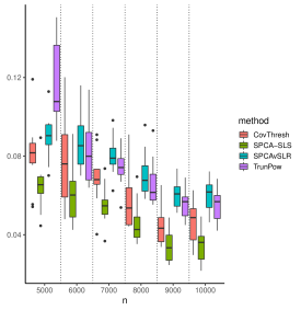
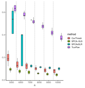
$(FP+FN)/2$

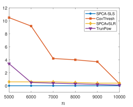
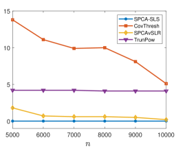
Figure 1: Estimation and support recovery error as available from different methods on synthetic data with $p=10000$ and different values of $n$ (along the x-axis), as discussed in the text (Section 5.1.2). The left panels show results with $s=5$ and right panels $s=10$. The top panels compare estimation performance and bottom ones compare support recovery. Our proposed approach results in high-quality estimation performance, and perfect support recovery.

5.1.3 Estimation with varying sparsity levels ($s$)

In this scenario, we fix $p=10,000$ and $n=7500$ and consider different sparsity levels $s\in\{5,7,10,12,15\}$. We compare our SPCA-SLS algorithm with competing methods outlined above. We use the same computational setup as in Section 5.1.2.

The results for this scenario (estimation and support recovery properties) are shown in Figure 2. As it can be seen, increasing $s$ results in worse statistical performance. However, our proposed approach continues to work better than other estimators in terms of estimation and support recovery.

	Estimation Error, $p=10^{4},n=7500$		Support Recovery, $p=10^{4},n=7500$
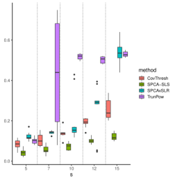
$|\sin\angle(\hat{u},u^{*})|$		$(FP+FN)/2$

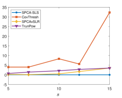
Figure 2: Numerical results for the synthetic dataset with $p=10000,n=7500$ in Section 5.1.3. The left panel shows the estimation performance and the right panel shows the support recovery performance.

5.1.4 A large-scale example with $p=20,000$

To show the scalability of our algorithm, we consider instances with $p=20,000$. We perform a set of experiments on a personal computer. We use a machine equipped with AMD Ryzen 9 5900X CPU $@$ 3.70GHz, using 32GB of RAM. However, in our experiments, Julia did not use more than 12GB of RAM. We set $p=20,000,s\in\{5,10\}$ and $n\in\{5000,10000,15000,20000\}$. The runtime of our methods is limited to 5 minutes.

In this case, we explore Algorithm 1 applied to two cases of Problem (26): (a) we consider the unregularized case $\lambda=0$ denoted by SPCA-SLS and (b) $\lambda>0$ chosen as in Section 5.1.1, denoted by SPCA-SLSR. We use (b) to demonstrate the effect of the perspective regularization in (26). The results for this case are shown in Figure 3, which compares the estimation performance of different algorithms. As it can be seen, our method leads to better estimation performance compared to other SPCA methods. Moreover, having $\lambda>0$ (in case of SPCA-SLSR) does not negatively affect the estimation performance of our method, while it helps to achieve stronger optimality certificates.

	$s=5$	$s=10$
$|\sin\angle(\hat{u},u^{*})|$

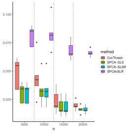
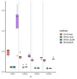
Figure 3: Numerical results for the synthetic dataset with $p=20000$ in Section 5.1.4. The left panel shows the statistical performance for $s=5$. The right panel shows the statistical performance for $s=10$.

5.2 Real dataset example

To show the scalability of our algorithm and to compare them with other well-known algorithms, we do further numerical experiments on the Gisette dataset (Guyon et al., 2005). This dataset is a handwritten digit recognition dataset with $n=6000$ samples and $p=5000$ features. We run SPCA-SLS, SPCA-SLSR (with $\lambda$ chosen as in Section 5.1.1), TrunPow, SPCAvSLR and CovTresh for this data matrix and two values of $s\in\{4,5\}$. Parameter selection is done similar to the synthetic data experiments in Section 5.1. We use the same personal computer from Section 5.1.4 with Julia process limited to 6GB of RAM usage. To compare the results of different methods, we plot the absolute values of estimated PCs and examine the sparsity pattern of the associated eigenvector. Figure 4 shows the results for two values of $s$ — interestingly, we observe that the sparsity patterns available from different algorithms are different, with CovTresh leading to a denser support.

$s=4$	$s=5$

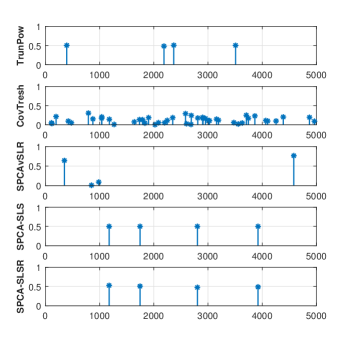
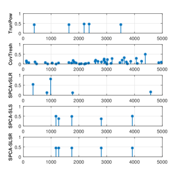
Figure 4: Comparison of estimated PCs by different algorithms for the real dataset in Section 5.2. The left panel shows the results for $s=4$ and the right panel shows the results for $s=5$. In both cases, SPCA-SLS reaches the optimality gap of less than $12\%$ and SPCA-SLSR reaches the optimality gap of less than $10\%$ after 10 minutes.

6 Conclusion

In this paper, we consider a discrete optimization-based approach for the SPCA problem under the spiked covariance model. We present a novel estimator given by the solution to a mixed integer second order conic optimization formulation. Different from prior work on MIP-based approaches for the SPCA problem, our formulation is based on the properties of the statistical model, which leads to notable improvements in computational performance. We analyze the statistical properties of our estimator: both estimation and variable selection properties. We present custom cutting plane algorithms for our optimization formulation that can obtain (near) optimal solutions for large problem instances with $p\approx 20000$ features. Our custom algorithms offer significant improvements in terms of runtime, scalability over off-the-shelf commercial MIP-solvers, and recently proposed MIP-based approaches for the SPCA problem. In addition, our numerical experiments appear to suggest that our method outperforms some well-known polynomial-time and heuristic algorithms for SPCA in terms of estimation error and support recovery.

Proofs and Technical Details

Appendix A Proofs of Main Results

Before proceeding with the proof of main results, we present an extended version of Lemma 1 that we use throughout the proofs.

Lemma 3.

Let $\varepsilon\in\mathbb{R}^{n\times p}$ be such that for $j\in[p]$,

$$\varepsilon_{:,j}=X_{:,j}-\sum_{i\neq j}\beta^{*}_{i,j}X_{:,i}.$$

Then, $\varepsilon_{:,j}$ and $\{X_{:,i}\}_{i\neq j}$ are independent for every $j$. Moreover, for every $j$,

$$\varepsilon_{:,j}\sim\mathcal{N}(0,(\sigma_{j}^{*})^{2}I_{n}).$$

A.1 Proof of Theorem 1

To prove this theorem, we first mention a few basic results that we use throughout the proof.

Lemma 4 (Theorem 1.19, Rigollet and Hütter (2015)).

Let $\omega\in\mathbb{R}^{p}$ be a random vector with $\omega_{i}\stackrel{{\scriptstyle\text{iid}}}{{\sim}}\mathcal{N}(0,\sigma^{2})$, then

$${\rm I}\kern-1.79993pt{\rm P}(\sup_{{\theta}\in\mathcal{B}(p)}{\theta}^{T}{\omega}>t)\leq\exp\left(-\frac{t^{2}}{8\sigma^{2}}+p\log 5\right),$$ (33)

where $\mathcal{B}(p)$ denotes the unit Euclidean ball of dimension $p$.

Lemma 5.

Suppose $X\in\mathbb{R}^{n\times p}$ (with $n\geq p$) be a data matrix with independent rows, with the $i$-th row distributed as $\mathcal{N}(0,G)$ (with positive definite $G$) where $0<\underline{\sigma}\leq\sqrt{\lambda_{\min}(G)}\leq\sqrt{\lambda_{\max}(G)}\leq\overline{\sigma}$. The following holds:

$$\underline{\sigma}\left(1-c_{0}\left(\sqrt{\frac{p}{n}}+\frac{t}{\sqrt{n}}\right)\right)\lesssim\frac{1}{\sqrt{n}}\sigma_{\min}(X)\leq\frac{1}{\sqrt{n}}\sigma_{\max}(X)\lesssim\overline{\sigma}\left(1+c_{0}\left(\sqrt{\frac{p}{n}}+\frac{t}{\sqrt{n}}\right)\right)$$

with probability at least $\geq 1-\exp(-Ct^{2})$ for some universal constants $C,c_{0}>0$.

Proof.

Let $G=USU^{T}$ be the eigendecomposition of $G$ with diagonal $S$ containing the eigenvalues of $G$. Let $Y=XUS^{-1/2}$. For any $i,j\in[n]$ such that $i\neq j$, we have:

$${\rm I}\kern-1.79993pt{\rm E}[Y_{i,:}^{T}Y_{i,:}]={\rm I}\kern-1.79993pt{\rm E}[S^{-1/2}U^{T}X_{i,:}^{T}X_{i,:}US^{-1/2}]=S^{-1/2}U^{T}GUS^{-1/2}=I_{p},$$

$$\text{and}~{}~{}~{}~{}{\rm I}\kern-1.79993pt{\rm E}[Y_{i,:}^{T}Y_{j,:}]={\rm I}\kern-1.79993pt{\rm E}[S^{-1/2}U^{T}X_{i,:}^{T}X_{j,:}US^{-1/2}]=0$$

showing that $Y\sim\mathcal{N}(0,{I}_{p})$. Therefore, by Theorem 4.6.1 of Vershynin (2018), the following holds

$$1-c_{0}\left(\sqrt{\frac{p}{n}}+\frac{t}{\sqrt{n}}\right)\lesssim\frac{1}{\sqrt{n}}\sigma_{\min}(Y)\leq\frac{1}{\sqrt{n}}\sigma_{\max}(Y)\lesssim 1+c_{0}\left(\sqrt{\frac{p}{n}}+\frac{t}{\sqrt{n}}\right)$$ (34)

with probability at least $\geq 1-\exp(-Ct^{2})$ for some universal constants $C,c_{0}>0$. Moreover,

$$\sigma_{\min}(X) =\inf_{\|z\|_{2}=1}\|Xz\|_{2}$$

$$=\inf_{\|z\|_{2}=1}\|YS^{1/2}U^{T}z\|_{2}$$

$$=\inf_{\|z\|_{2}=1}\|YS^{1/2}z\|_{2}$$

$$=\inf_{\|z\|_{2}=1}\|S^{1/2}z\|_{2}\left\|Y\frac{S^{1/2}z}{\|S^{1/2}z\|_{2}}\right\|_{2}$$

$$\geq\sqrt{\lambda_{\min}(G)}~{}\sigma_{\min}(Y).$$

Combining the above with (34), we arrive at the first inequality in this lemma. The proof for the third inequality follows by an argument similar to the above, but for $\sigma_{\max}$. ∎

Lemma 6.

Suppose the rows of the matrix $X\in\mathbb{R}^{n\times p}$ are iid draws from a multivariate Gaussian distribution $\mathcal{N}(0,G)$. Moreover, suppose for any $S\subseteq[p]$ such that $|S|\leq s$,

$$\lambda_{\min}(G_{S,S})\geq\kappa^{2}>0.$$

Then, if $n\gtrsim s\log p$, with probability at least $1-s\exp(-10s\log p)$, we have:

$$\sigma_{\min}(X_{S})\gtrsim\kappa\sqrt{n}~{}~{}~{}\text{for all $S$ with $|S|\leq s$}.$$

(We recall that $X_{S}$ is a sub-matrix of $X$ restricted to the columns indexed by $S$).

Proof.

Suppose $S$ is fixed. Take $t=\sqrt{cs\log(p)}$ for some constant $c>0$. By Lemma 5, with probability greater than $1-\exp(-Ccs\log(p))$

$$\frac{1}{\sqrt{n}}\sigma_{\min}(X_{S})\gtrsim\kappa\left(1-c_{0}\left(\sqrt{\frac{|S|}{n}}+\sqrt{\frac{cs\log p}{n}}\right)\right)\gtrsim\kappa\left(1-c_{0}(1+\sqrt{c})\sqrt{\frac{s\log p}{n}}\right).$$

We consider a union bound over all possible sets $S$ (of size at most $s$):

$$1-\sum_{k\leq s}\sum_{|S|=k}\exp(-Ccs\log(p)) \geq 1-\sum_{k\leq s}{p\choose k}\exp(-Ccs\log(p))$$

$$\stackrel{{\scriptstyle(a)}}{{\geq}}1-\sum_{k\leq s}\left(\frac{ep}{k}\right)^{k}\exp(-Ccs\log(p))$$

$$\geq 1-\sum_{k\leq s}\left(ep\right)^{s}\exp(-Ccs\log(p))$$

$$=1-s\exp(-Ccs\log p+s\log(ep))$$

where $(a)$ is due to the inequality ${p\choose k}\leq\left(\frac{ep}{k}\right)^{k}$.

Therefore, with probability greater than $1-s\exp(-Ccs\log p+s\log(ep))$, we have

$$\frac{1}{\sqrt{n}}\sigma_{\min}(X_{S})\gtrsim\kappa\left(1-c_{0}(1+\sqrt{c})\sqrt{\frac{s\log p}{n}}\right)~{}~{}~{}\text{for all $S\subset[p]$ with $|S|\leq s$}.$$

Finally, the result follows by choosing $c$ large enough to have $-Ccs\log p+s\log(ep)<-10s\log p$ and $n$ such that $n>2c_{0}^{2}(1+\sqrt{c})^{2}s\log p.$

∎

Lemma 7.

For fixed $j_{1},j_{2}\in[p]$, and $n>\frac{2}{C_{b}}\log(1/\delta)$, we have

$${\rm I}\kern-1.79993pt{\rm P}\left(\left|\frac{1}{n}\sum_{i=1}^{n}X_{i,j_{1}}X_{i,j_{2}}-G^{*}_{j_{1},j_{2}}\right|>c_{\psi}\sqrt{\frac{\log(1/\delta)}{C_{b}n}}\right)\leq 2\delta$$ (35)

for some universal constants $C_{b},c_{\psi}>0$ (We recall that $G^{*}$ is the spiked covariance matrix from (1)).

Proof.

Suppose $i\in[n]$ and $j_{1},j_{2}\in[p]$. We have $|{\rm I}\kern-1.79993pt{\rm E}[X_{i,j_{1}}X_{i,j_{2}}]|=|G^{*}_{j_{1},j_{2}}|\leq 2$ and ${\rm I}\kern-1.79993pt{\rm E}[X_{i,j_{1}}]=0$. As a result, by Bernstein’s inequality (Vershynin, 2018, Theorem 2.8.1), we have

$${\rm I}\kern-1.79993pt{\rm P}\left(\left|\frac{1}{n}\sum_{i=1}^{n}X_{i,j_{1}}X_{i,j_{2}}-G^{*}_{j_{1},j_{2}}\right|>t\right)\leq 2\exp\left(-C_{b}n((t/c_{\psi})^{2}\land(t/c_{\psi}))\right)$$ (36)

for some universal constants $c_{\psi},C_{b}>0$. Therefore, if $n>\frac{2}{C_{b}}\log(\frac{1}{\delta})$ and $t=c_{\psi}\sqrt{\frac{\log(1/\delta)}{C_{b}n}}$, we have:

$$\frac{t}{c_{\psi}}=\sqrt{\frac{\log(1/\delta)}{C_{b}n}}<1$$

which implies $(t/c_{\psi})^{2}\land(t/c_{\psi})=(t/c_{\psi})^{2}$. As a result, from (36), we arrive at (35). ∎

The proof of Theorem 1 is based on the following technical lemma.

Lemma 8.

Under the assumptions of Theorem 1, one has

$$\frac{1}{n}\sum_{j=1}^{p}\left[\left\|\sum_{i\neq j}(\hat{\beta}_{i,j}-\beta_{i,j}^{*})X_{:,i}\right\|_{2}^{2}\right] \lesssim\frac{s^{2}\log(p/s)}{n}+\frac{1}{n}\sum_{j=1}^{p}\left\|\sum_{i\neq j}(\beta^{*}_{i,j}-\tilde{\beta}_{i,j})X_{:,i}\right\|_{2}^{2}$$

with probability greater than $1-2s\exp(-10s\log(p/s))$.

Proof.

Let $\beta_{i,j}^{*}=-\frac{({(G^{*})}^{-1})_{j,i}}{({(G^{*})}^{-1})_{j,j}}$ be the true regression coefficients.

By taking $z$ to represent the support of $\tilde{u}$ and noting that $\beta^{*}_{i,j}=\tilde{\beta}_{i,j}$ for $i,j\in\tilde{S}$, we can see that the matrix $\{\tilde{\beta}_{i,j}\}$ is feasible for Problem (7).

Using the optimality of $\hat{\beta}$ and feasibility of $\tilde{\beta}$ for Problem (7), we have:

$$\sum_{j=1}^{p}\left\|X_{:,j}-\sum_{i\neq j}\hat{\beta}_{i,j}X_{:,i}\right\|_{2}^{2}\leq\sum_{j=1}^{p}\left\|X_{:,j}-\sum_{i\neq j}\tilde{\beta}_{i,j}X_{:,i}\right\|_{2}^{2}$$

$$\Rightarrow \sum_{j=1}^{p}\left[\left\|\sum_{i\neq j}(\hat{\beta}_{i,j}-\beta_{i,j}^{*})X_{:,i}\right\|_{2}^{2}-\left\|\sum_{i\neq j}(\tilde{\beta}_{i,j}-\beta_{i,j}^{*})X_{:,i}\right\|_{2}^{2}\right]\leq 2\sum_{j=1}^{p}{\varepsilon}_{:,j}^{T}\left(\sum_{i\neq j}(\hat{\beta}_{i,j}-\tilde{\beta}_{i,j})X_{:,i}\right)$$ (37)

where we used the representation $X_{:,j}=\sum_{i\neq j}\beta^{*}_{i,j}X_{:,i}+\varepsilon_{:,j}$ by Lemma 3. By the inequality $2ab\leq 4a^{2}+b^{2}/4$,

$$2{\varepsilon}_{:,j}^{T}\left(\sum_{i\neq j}(\hat{\beta}_{i,j}-\tilde{\beta}_{i,j}){X}_{:,i}\right) =2{\varepsilon}_{:,j}^{T}\frac{\sum_{i\neq j}(\hat{\beta}_{i,j}-\tilde{\beta}_{i,j})X_{:,i}}{\|\sum_{i\neq j}(\hat{\beta}_{i,j}-\tilde{\beta}_{i,j})X_{:,i}\|_{2}}\|\sum_{i\neq j}(\hat{\beta}_{i,j}-\tilde{\beta}_{i,j})X_{:,i}\|_{2}$$

$$\leq 4\left[{\varepsilon}_{:,j}^{T}\frac{\sum_{i\neq j}(\hat{\beta}_{i,j}-\tilde{\beta}_{i,j})X_{:,i}}{\|\sum_{i\neq j}(\hat{\beta}_{i,j}-\tilde{\beta}_{i,j})X_{:,i}\|_{2}}\right]^{2}+\frac{1}{4}\|\sum_{i\neq j}(\hat{\beta}_{i,j}-\tilde{\beta}_{i,j})X_{:,i}\|_{2}^{2}.$$ (38)

In addition,

$$\frac{1}{4}\|\sum_{i\neq j}(\hat{\beta}_{i,j}-\tilde{\beta}_{i,j})X_{:,i}\|_{2}^{2}\leq\frac{1}{2}\|\sum_{i\neq j}(\hat{\beta}_{i,j}-\beta^{*}_{i,j})X_{:,i}\|_{2}^{2}+\frac{1}{2}\|\sum_{i\neq j}(\beta^{*}_{i,j}-\tilde{\beta}_{i,j})X_{:,i}\|_{2}^{2}.$$ (39)

Substituting (38) and (39) into (37),

$$\sum_{j=1}^{p}\left\|\sum_{i\neq j}(\hat{\beta}_{i,j}-\beta_{i,j}^{*})X_{:,i}\right\|_{2}^{2}\leq 8\sum_{j=1}^{p}\left[{\varepsilon}_{:,j}^{T}\frac{\sum_{i\neq j}(\hat{\beta}_{i,j}-\tilde{\beta}_{i,j})X_{:,i}}{\|\sum_{i\neq j}(\hat{\beta}_{i,j}-\tilde{\beta}_{i,j})X_{:,i}\|_{2}}\right]^{2}+3\sum_{j=1}^{p}\left\|\sum_{i\neq j}(\beta^{*}_{i,j}-\tilde{\beta}_{i,j})X_{:,i}\right\|_{2}^{2}.$$ (40)

For convenience, let us introduce the following notation:

$$\hat{y}^{(j)} =\sum_{i\neq j}(\hat{\beta}_{i,j}-\tilde{\beta}_{i,j})X_{:,i},$$ (41)

$$\hat{S} =S(\hat{z})\cup S(\tilde{u}).$$ (42)

Note that $|\hat{S}|\leq 2s$. In the rest of the proof, ${\rm I}\kern-1.79993pt{\rm P}(\cdot)$ denotes the probability w.r.t. the data matrix $X$ (which includes $\varepsilon$). Note that $\hat{\beta}_{i,j}-\tilde{\beta}_{i,j}$ can be nonzero only if $i,j\in\hat{S}$ (as $\hat{\beta}_{i,j},\tilde{\beta}_{i,j}$ can be nonzero for $i,j\in S(\hat{z})$ and $i,j\in S(\tilde{u})$, respectively) so $\hat{y}^{(j)}=0$ for $j\notin\hat{S}$. As a result, one has

$${\rm I}\kern-1.79993pt{\rm P}\left(\sum_{j=1}^{p}\left[\varepsilon_{:,j}^{T}\frac{\hat{y}^{(j)}}{\|\hat{y}^{(j)}\|_{2}}\right]^{2}>t\right) ={\rm I}\kern-1.79993pt{\rm P}\left(\sum_{j\in\hat{S}}\left[\varepsilon_{:,j}^{T}\frac{\hat{y}^{(j)}}{\|\hat{y}^{(j)}\|_{2}}\right]^{2}>t\right)$$

$$\leq{\rm I}\kern-1.79993pt{\rm P}\left(\max_{\begin{subarray}{c}S\subseteq[p]\\ |S|=2s\end{subarray}}\sum_{j\in S}\sup_{\begin{subarray}{c}v\in\mathbb{R}^{p}\\ S(v)=S\end{subarray}}\left[\varepsilon_{:,j}^{T}\frac{\sum_{i\neq j}v_{i}X_{:,i}}{\|\sum_{i\neq j}v_{i}X_{:,i}\|_{2}}\right]^{2}>t\right)$$ (43)

where the inequality (43) takes into account the definition of $\hat{y}^{(j)}$ in (41) and the observation that

$$\sum_{j\in\hat{S}}\left[\varepsilon_{:,j}^{T}\frac{\hat{y}^{(j)}}{\|\hat{y}^{(j)}\|_{2}}\right]^{2}\leq\sum_{j\in\hat{S}}\sup_{\begin{subarray}{c}v\in\mathbb{R}^{p}\\ S(v)=\hat{S}\end{subarray}}\left[\varepsilon_{:,j}^{T}\frac{\sum_{i\neq j}v_{i}X_{:,i}}{\|\sum_{i\neq j}v_{i}X_{:,i}\|_{2}}\right]^{2}.$$

Let $\mathbb{X}^{(j)}\in\mathbb{R}^{n\times(p-1)}$ be the matrix $X$ with column $j$ removed. Let $\Phi_{S}\in\mathbb{R}^{n\times|S|}$ be an orthonormal basis for the linear space spanned by $X_{:,i}$, $i\in S$ for $S\subseteq[p]$. For a fixed set $S$ and $j\in S$, and $t>0$,

$${\rm I}\kern-1.79993pt{\rm P}\left(\sup_{\begin{subarray}{c}v\in\mathbb{R}^{p}\\ S(v)=S\end{subarray}}\left[\varepsilon_{:,j}^{T}\frac{\sum_{i\neq j}v_{i}X_{:,i}}{\|\sum_{i\neq j}v_{i}X_{:,i}\|_{2}}\right]^{2}>t\right) \stackrel{{\scriptstyle(a)}}{{=}}{\rm I}\kern-1.79993pt{\rm P}\left(\left.\sup_{\begin{subarray}{c}v\in\mathbb{R}^{p}\\ S(v)=S\end{subarray}}\left[\varepsilon_{:,j}^{T}\frac{\sum_{i\neq j}v_{i}{X}_{:,i}}{\|\sum_{i\neq j}v_{i}X_{:,i}\|_{2}}\right]^{2}>t\right|\mathbb{X}^{(j)}\right)$$

$$\stackrel{{\scriptstyle(b)}}{{\leq}}{\rm I}\kern-1.79993pt{\rm P}\left(\left.\sup_{\alpha\in\mathcal{B}(|S\setminus\{j\}|)}\left[\varepsilon_{:,j}^{T}\Phi_{S\setminus\{j\}}\alpha\right]^{2}>t\right|\mathbb{X}^{(j)}\right)$$

$$\leq{\rm I}\kern-1.79993pt{\rm P}\left(\left.\sup_{{\alpha}\in\mathcal{B}(|S\setminus\{j\}|)}\left[\varepsilon_{:,j}^{T}{\Phi}_{S\setminus\{j\}}{\alpha}\right]>\sqrt{t}\right|\mathbb{X}^{(j)}\right)$$

$$\stackrel{{\scriptstyle(c)}}{{\leq}}\exp\left(-\frac{t}{8({\sigma^{*}_{j}})^{2}}+|S\setminus\{j\}|\log 5\right)$$

$$\stackrel{{\scriptstyle(d)}}{{\leq}}\exp\left(-\frac{t}{16}+2s\log 5\right)$$ (44)

where $(a)$ is due to the independence of $\varepsilon_{:,j}$ and $\mathbb{X}^{(j)}$ from Lemma 3, $(b)$ is due to the fact that $\sum_{i\neq j}v_{i}X_{:,i}$ is in the column span of $\Phi_{S\setminus\{j\}}$, $(c)$ is due to Lemma 4 and the conditional distribution $\Phi_{S\setminus\{j\}}^{T}\varepsilon_{:,j}|\mathbb{X}^{(j)}\stackrel{{\scriptstyle}}{{\sim}}\mathcal{N}(0,({\sigma_{j}^{*}})^{2}I_{|S|-1})$, and $(d)$ is due to $|S|\leq 2s$ and $({\sigma_{j}^{*}})^{2}\leq 2$. Therefore, by taking

$$t_{1}=c_{1}s\log(p/s)+16\log(1/\delta)$$

with $c_{1}=32\log 5$ in (44), we get

$${\rm I}\kern-1.79993pt{\rm P}\left(\sup_{\begin{subarray}{c}v\in\mathbb{R}^{p}\\ S(v)=S\end{subarray}}\left[\varepsilon_{:,j}^{T}\frac{\sum_{i\neq j}v_{i}X_{:,i}}{\|\sum_{i\neq j}v_{i}X_{:,i}\|_{2}}\right]^{2}>t_{1}\right)\leq\exp\left(-2s\log 5\log(p/s)+\log\delta+2s\log 5\right)\leq\delta,$$ (45)

where in the second inequality in (45) we used the assumption $p/s\geq 5>e$. Therefore, by taking $t=2c_{1}s^{2}\log(p/s)+32s\log(1/\delta)$ and

$$\delta=\exp(-(10+e)s\log(2p/s)),$$ (46)

we have

$${\rm I}\kern-1.79993pt{\rm P}\left(\sum_{j=1}^{p}\left[\varepsilon_{:,j}^{T}\frac{\hat{y}^{(j)}}{\|\hat{y}^{(j)}\|_{2}}\right]^{2}>t\right) \stackrel{{\scriptstyle(a)}}{{\leq}}{\rm I}\kern-1.79993pt{\rm P}\left(\max_{\begin{subarray}{c}S\subseteq[p]\\ |S|=2s\end{subarray}}\sum_{j\in S}\sup_{\begin{subarray}{c}v\in\mathbb{R}^{p}\\ S(v)=S\end{subarray}}\left[\varepsilon_{:,j}^{T}\frac{\sum_{i\neq j}v_{i}X_{:,i}}{\|\sum_{i\neq j}v_{i}X_{:,i}\|_{2}}\right]^{2}>t\right)$$

$$\stackrel{{\scriptstyle(b)}}{{\leq}}\sum_{\begin{subarray}{c}S\subseteq[p]\\ |S|=2s\end{subarray}}{\rm I}\kern-1.79993pt{\rm P}\left(\sum_{j\in S}\sup_{\begin{subarray}{c}v\in\mathbb{R}^{p}\\ S(v)=S\end{subarray}}\left[\varepsilon_{:,j}^{T}\frac{\sum_{i\neq j}v_{i}X_{:,i}}{\|\sum_{i\neq j}v_{i}X_{:,i}\|_{2}}\right]^{2}>t\right)$$

$$\stackrel{{\scriptstyle(c)}}{{\leq}}\sum_{\begin{subarray}{c}S\subseteq[p]\\ |S|=2s\end{subarray}}{\rm I}\kern-1.79993pt{\rm P}\left(\exists j\in S:\sup_{\begin{subarray}{c}v\in\mathbb{R}^{p}\\ S(v)=S\end{subarray}}\left[\varepsilon_{:,j}^{T}\frac{\sum_{i\neq j}v_{i}X_{:,i}}{\|\sum_{i\neq j}v_{i}X_{:,i}\|_{2}}\right]^{2}>t_{1}\right)$$

$$\stackrel{{\scriptstyle(d)}}{{\leq}}\sum_{\begin{subarray}{c}S\subseteq[p]\\ |S|=2s\end{subarray}}\sum_{j\in S}{\rm I}\kern-1.79993pt{\rm P}\left(\sup_{\begin{subarray}{c}v\in\mathbb{R}^{p}\\ S(v)=S\end{subarray}}\left[\varepsilon_{:,j}^{T}\frac{\sum_{i\neq j}v_{i}X_{:,i}}{\|\sum_{i\neq j}v_{i}X_{:,i}\|_{2}}\right]^{2}>t_{1}\right)$$

$$\stackrel{{\scriptstyle(e)}}{{\leq}}2s{p\choose 2s}\delta$$

$$\stackrel{{\scriptstyle(f)}}{{\leq}}2s\left(\frac{ep}{2s}\right)^{2s}\delta$$

$$\stackrel{{\scriptstyle(g)}}{{\leq}}2s\left(\frac{2p}{s}\right)^{es}\delta$$

$$=2s\exp(-10s\log(2p/s))$$

$$\leq 2s\exp(-10s\log(p/s)),$$ (47)

where $(a)$ is due to (43), $(b),(d)$ are true because of union bound, $(c)$ follows by noting that: for $j\in S$, if

$$\sup_{\begin{subarray}{c}v\in\mathbb{R}^{p}\\ S(v)=S\end{subarray}}\left[\varepsilon_{:,j}^{T}\frac{\sum_{i\neq j}v_{i}X_{:,i}}{\|\sum_{i\neq j}v_{i}X_{:,i}\|_{2}}\right]^{2}<t_{1},$$

then

$$\sum_{j\in S}\sup_{\begin{subarray}{c}v\in\mathbb{R}^{p}\\ S(v)=S\end{subarray}}\left[\varepsilon_{:,j}^{T}\frac{\sum_{i\neq j}v_{i}X_{:,i}}{\|\sum_{i\neq j}v_{i}X_{:,i}\|_{2}}\right]^{2}<2st_{1}=t.$$

Inequality $(e)$ above, is due to (45) and the fact that $|S|=2s$, $(f)$ is due to the inequality ${p\choose 2s}\leq(ep/2s)^{2s}$ and $(g)$ is true as $e>2$. By (40) and (47), and substituting $\delta$ from (46),

$$\sum_{j=1}^{p}\left[\left\|\sum_{i\neq j}(\hat{\beta}_{i,j}-\beta_{i,j}^{*})X_{:,i}\right\|_{2}^{2}\right] \lesssim{s^{2}\log(p/s)}+\sum_{j=1}^{p}\left\|\sum_{i\neq j}(\beta^{*}_{i,j}-\tilde{\beta}_{i,j})X_{:,i}\right\|_{2}^{2}$$

with the probability greater than $1-2s\exp(-10s\log(p/s))$. ∎

Proof of Theorem 1.

Let $\mathbb{X}^{(j)}\in\mathbb{R}^{n\times(p-1)}$ be the matrix $X$ with column $j$ removed. Let us define the following events:

$$\mathcal{A} =\left\{\max_{j_{1},j_{2}\in[p]}~{}\frac{1}{n}|X_{:,j_{1}}^{T}X_{:,j_{2}}|\leq 3\right\},$$ (48)

$$\mathcal{E}_{j} =\left\{\mathbb{X}^{(j)}:\sigma_{\min}(\mathbb{X}^{(j)}_{:,S})\geq c_{r}\sqrt{n}\,\,\,\forall S\subseteq[p-1],|S|\leq 2s\right\},~{}j\in[p]$$

for some constant $c_{r}>0$. From (35) for fixed $j_{1},j_{2}\in[p]$, with probability at least $1-2\delta$, we have:

$$\frac{1}{n}|X_{:,j_{1}}^{T}X_{:,j_{2}}|\leq|G^{*}_{j_{1},j_{2}}|+c_{\psi}\sqrt{\frac{\log(1/\delta)}{C_{b}n}}.$$ (49)

Let $\delta=p^{-10}$ and $n>10c_{\psi}^{2}\log p/{C_{b}}$. Noting that $|G^{*}_{j_{1},j_{2}}|\leq 2$ for all $j_{1},j_{2}$, and by a union bound over all $j_{1},j_{2}\in[p]$, the following holds true

$${\rm I}\kern-1.79993pt{\rm P}\left(\mathcal{A}\right)>1-2p^{-8}.$$ (50)

Note that for any $S\subseteq[p]$, with $1\leq|S|\leq 2s$,

$$\lambda_{\min}\left(G^{*}_{{S},{S}}\right)=\lambda_{\min}\left(I_{|{S}|}+\theta u^{*}_{{S}}({u^{*}_{{S}}})^{T}\right)\geq 1.$$

Hence, by Lemma 6, as $n\gtrsim s\log p$,

$${\rm I}\kern-1.79993pt{\rm P}(\mathcal{E}_{j})\geq 1-2s\exp(-20s\log(p-1)).$$

For the rest of the proof, we assume $\mathcal{A},\mathcal{E}_{j}$ (for all $j\in[p]$) and the event of Lemma 8 hold true. Note that the intersection of these events holds true with probability at least

$$1-2p^{-8}-2sp\exp(-20s\log(p-1))-2s\exp(-10s\log(p/s))$$ (51)

by union bound.
Let $\hat{S}=S(\hat{z})\cup S(\tilde{u})$. Recall that $\hat{\beta}_{i,j}=0$ for all $i\notin\hat{S}$. We have the following:

$$\left\|\sum_{i:i\neq j}(\hat{\beta}_{i,j}-\beta_{i,j}^{*})X_{:,i}\right\|_{2}^{2} =\left\|\sum_{i\in\hat{S}}(\hat{\beta}_{i,j}-\beta_{i,j}^{*})X_{:,i}+\sum_{i\notin\hat{S}}(\hat{\beta}_{i,j}-\beta_{i,j}^{*})X_{:,i}\right\|_{2}^{2}$$

$$=\left\|\sum_{i\in\hat{S}}(\hat{\beta}_{i,j}-\beta_{i,j}^{*})X_{:,i}\right\|_{2}^{2}+\left\|\sum_{i\notin\hat{S}}\beta_{i,j}^{*}X_{:,i}\right\|_{2}^{2}-2\sum_{\begin{subarray}{c}i_{1}\notin\hat{S}\\ i_{2}\in\hat{S}\end{subarray}}\beta^{*}_{i_{1},j}(\hat{\beta}_{i_{2},j}-\beta^{*}_{i_{2},j})X_{:,i_{1}}^{T}X_{:,i_{2}}$$

$$\geq\left\|\sum_{i\in\hat{S}}(\hat{\beta}_{i,j}-\beta_{i,j}^{*})X_{:,i}\right\|_{2}^{2}-2\sum_{\begin{subarray}{c}i_{1}\notin\hat{S}\\ i_{2}\in\hat{S}\end{subarray}}|\beta^{*}_{i_{1},j}||\hat{\beta}_{i_{2},j}-\beta^{*}_{i_{2},j}||X_{:,i_{1}}^{T}X_{:,i_{2}}|.$$ (52)

Next, note that

$$2\sum_{\begin{subarray}{c}i_{1}\notin\hat{S}\\ i_{2}\in\hat{S}\end{subarray}}|\beta^{*}_{i_{1},j}||\hat{\beta}_{i_{2},j}-\beta^{*}_{i_{2},j}||X_{:,i_{1}}^{T}X_{:,i_{2}}| =2\sum_{\begin{subarray}{c}i_{1}\notin\hat{S}\\ i_{2}\in\hat{S}\end{subarray}}\sqrt{|\beta^{*}_{i_{1},j}|}\sqrt{|\beta^{*}_{i_{1},j}|}|\hat{\beta}_{i_{2},j}-\beta^{*}_{i_{2},j}||X_{:,i_{1}}^{T}X_{:,i_{2}}|$$

$$\stackrel{{\scriptstyle(a)}}{{\leq}}\sum_{\begin{subarray}{c}i_{1}\notin\hat{S}\\ i_{2}\in\hat{S}\end{subarray}}\left(c_{\beta}|\beta^{*}_{i_{1},j}|+\frac{1}{c_{\beta}}|\beta^{*}_{i_{1},j}||\hat{\beta}_{i_{2},j}-\beta^{*}_{i_{2},j}|^{2}\right)|X_{:,i_{1}}^{T}X_{:,i_{2}}|$$

$$\stackrel{{\scriptstyle(b)}}{{\leq}}\frac{4n}{c_{\beta}}\sum_{i_{1}\notin\hat{S}}|\beta^{*}_{i_{1},j}|\sum_{i_{2}\neq j}(\beta_{i_{2},j}^{*}-\hat{\beta}_{i_{2},j})^{2}+c_{\beta}\sum_{\begin{subarray}{c}i_{1}\notin\hat{S}\\ i_{2}\in\hat{S}\end{subarray}}|\beta^{*}_{i_{1},j}||X_{:,i_{1}}^{T}X_{:,i_{2}}|$$

$$\stackrel{{\scriptstyle(c)}}{{\leq}}\frac{4n}{c_{\beta}}\sum_{i:i\neq j}(\beta_{i,j}^{*}-\hat{\beta}_{i,j})^{2}+c_{\beta}\sum_{\begin{subarray}{c}i_{1}\notin\hat{S}\\ i_{2}\in\hat{S}\end{subarray}}|\beta^{*}_{i_{1},j}||X_{:,i_{1}}^{T}X_{:,i_{2}}|,$$ (53)

for some sufficiently large constant $c_{\beta}>0$ (that we discuss later), where $(a)$ is due to the inequality $2ab\leq c_{\beta}a^{2}+b^{2}/c_{\beta}$, $(b)$ is due to event $\mathcal{A}$ defined in (48) and $(c)$ is true as we assumed $\sum_{i\notin\hat{S}}|\beta^{*}_{i,j}|\leq 1$. As a result, from (52) and (53),

$$\left\|\sum_{i:i\neq j}(\hat{\beta}_{i,j}-\beta_{i,j}^{*})X_{:,i}\right\|_{2}^{2}\geq\left\|\sum_{i\in\hat{S}}(\hat{\beta}_{i,j}-\beta_{i,j}^{*})X_{:,i}\right\|_{2}^{2}-\frac{4n}{c_{\beta}}\sum_{i:i\neq j}(\beta_{i,j}^{*}-\hat{\beta}_{i,j})^{2}-c_{\beta}\sum_{\begin{subarray}{c}i_{1}\notin\hat{S}\\ i_{2}\in\hat{S}\end{subarray}}|\beta^{*}_{i_{1},j}||X_{:,i_{1}}^{T}X_{:,i_{2}}|.$$ (54)

On event $\mathcal{E}_{j}$ for $j\in[p]$,

$$\frac{1}{n}\left\|\sum_{i\in\hat{S}}(\hat{\beta}_{i,j}-\beta^{*}_{i,j})X_{:,i}\right\|_{2}^{2} =\frac{1}{n}\left\|X_{\hat{S}}(\hat{\beta}_{\hat{S},j}-\beta^{*}_{\hat{S},j})\right\|_{2}^{2}$$

$$\geq\frac{1}{n}\sigma_{\min}\left(\mathbb{X}^{(j)}_{:,\hat{S}\setminus\{j\}}\right)^{2}\left\|\hat{\beta}_{\hat{S}\setminus\{j\},j}-\beta^{*}_{\hat{S}\setminus\{j\},j}\right\|_{2}^{2}$$

$$\geq c_{r}\left\|\hat{\beta}_{\hat{S},j}-\beta^{*}_{\hat{S},j}\right\|_{2}^{2}$$

$$\geq c_{r}\sum_{i\in\hat{S}}(\hat{\beta}_{i,j}-\beta^{*}_{i,j})^{2},$$ (55)

where in the first inequality, we used the convention $\beta^{*}_{j,j}=\hat{\beta}_{j,j}=0$. As a result, for $j\in[p]$

$$\frac{1}{n}\left\|\sum_{i:i\neq j}(\hat{\beta}_{i,j}-\beta_{i,j}^{*})X_{:,i}\right\|_{2}^{2} \stackrel{{\scriptstyle(a)}}{{\geq}}\frac{1}{n}\left\|\sum_{i\in\hat{S}}(\hat{\beta}_{i,j}-\beta_{i,j}^{*})X_{:,i}\right\|_{2}^{2}-\frac{c_{\beta}}{n}\sum_{\begin{subarray}{c}i_{1}\notin\hat{S}\\ i_{2}\in\hat{S}\end{subarray}}|\beta^{*}_{i_{1},j}||X_{:,i_{1}}^{T}X_{:,i_{2}}|-\frac{4}{c_{\beta}}\sum_{i:i\neq j}(\beta_{i,j}^{*}-\hat{\beta}_{i,j})^{2}$$

$$\stackrel{{\scriptstyle(b)}}{{\geq}}c_{r}\sum_{i\in\hat{S}}(\hat{\beta}_{i,j}-\beta^{*}_{i,j})^{2}-\frac{c_{\beta}}{n}\sum_{\begin{subarray}{c}i_{1}\notin\hat{S}\\ i_{2}\in\hat{S}\end{subarray}}|\beta^{*}_{i_{1},j}||X_{:,i_{1}}^{T}X_{:,i_{2}}|-\frac{4}{c_{\beta}}\sum_{i:i\neq j}(\beta_{i,j}^{*}-\hat{\beta}_{i,j})^{2}$$

$$\stackrel{{\scriptstyle(c)}}{{\gtrsim}}\sum_{i\in\hat{S}}(\hat{\beta}_{i,j}-\beta^{*}_{i,j})^{2}-\sum_{\begin{subarray}{c}i_{1}\notin\hat{S}\\ i_{2}\in\hat{S}\end{subarray}}|\beta^{*}_{i_{1},j}|$$

$$\stackrel{{\scriptstyle(d)}}{{\gtrsim}}\sum_{i\in\hat{S}}(\hat{\beta}_{i,j}-\beta^{*}_{i,j})^{2}-s\sum_{i\notin\hat{S}}|\beta^{*}_{i,j}|$$

$$\stackrel{{\scriptstyle(e)}}{{\gtrsim}}\sum_{i\in\hat{S}}(\hat{\beta}_{i,j}-\beta^{*}_{i,j})^{2}-s\sum_{i:i\neq j}|\tilde{\beta}_{i,j}-\beta^{*}_{i,j}|$$ (56)

where $(a)$ is due to (54), $(b)$ is due to (55) and (50), $(c)$ is by taking $16/c_{r}>c_{\beta}>8/c_{r}$, $(d)$ is true because $|\hat{S}|\leq 2s$ and $(e)$ is true as $\tilde{\beta}_{i,j}=0$ for $i\notin\hat{S}$. Therefore,

$$\sum_{j=1}^{p}\sum_{i:i\neq j}(\hat{\beta}_{i,j}-\beta^{*}_{i,j})^{2} =\sum_{j=1}^{p}\sum_{i\in\hat{S}}(\hat{\beta}_{i,j}-\beta^{*}_{i,j})^{2}+\sum_{j=1}^{p}\sum_{i\notin\hat{S}}(\beta^{*}_{i,j})^{2}$$

$$\stackrel{{\scriptstyle(a)}}{{=}}\sum_{j=1}^{p}\sum_{i\in\hat{S}}(\hat{\beta}_{i,j}-\beta^{*}_{i,j})^{2}+\sum_{j=1}^{p}\sum_{i\notin\hat{S}}(\tilde{\beta}_{i,j}-\beta^{*}_{i,j})^{2}$$

$$\stackrel{{\scriptstyle(b)}}{{\lesssim}}\frac{1}{n}\sum_{j=1}^{p}\left\|\sum_{i:i\neq j}(\hat{\beta}_{i,j}-\beta_{i,j}^{*})X_{:,i}\right\|_{2}^{2}+\sum_{j=1}^{p}\sum_{i:i\neq j}\left[(\tilde{\beta}_{i,j}-\beta^{*}_{i,j})^{2}+s|\tilde{\beta}_{i,j}-\beta^{*}_{i,j}|\right]$$ (57)

where $(a)$ is true as $\tilde{\beta}_{i,j}=0$ for $i\notin\hat{S}$ and $(b)$ is true because of (56). In addition,

$$\sum_{j=1}^{p}\left\|\sum_{i:i\neq j}(\beta^{*}_{i,j}-\tilde{\beta}_{i,j})X_{:,i}\right\|_{2}^{2} \leq\sum_{j=1}^{p}\left[\sum_{i:i\neq j}|\beta^{*}_{i,j}-\tilde{\beta}_{i,j}|\|X_{:,i}\|_{2}\right]^{2}$$

$$\lesssim n\sum_{j=1}^{p}\left[\sum_{i:i\neq j}|\beta^{*}_{i,j}-\tilde{\beta}_{i,j}|\right]^{2}$$

$$\lesssim n\left[\sum_{j=1}^{p}\sum_{i:i\neq j}|\beta^{*}_{i,j}-\tilde{\beta}_{i,j}|\right]^{2}$$ (58)

where above, we used event $\mathcal{A}$ to arrive at the second inequality. Starting with (57), we arrive at the following:

$$\sum_{j=1}^{p}\sum_{i:i\neq j}(\hat{\beta}_{i,j}-\beta^{*}_{i,j})^{2} {\lesssim}\frac{1}{n}\sum_{j=1}^{p}\left\|\sum_{i:i\neq j}(\hat{\beta}_{i,j}-\beta_{i,j}^{*})X_{:,i}\right\|_{2}^{2}+\sum_{j=1}^{p}\sum_{i:i\neq j}\left[(\tilde{\beta}_{i,j}-\beta^{*}_{i,j})^{2}+s|\tilde{\beta}_{i,j}-\beta^{*}_{i,j}|\right]$$

$$\stackrel{{\scriptstyle(a)}}{{\lesssim}}\frac{s^{2}\log(p/s)}{n}+\frac{1}{n}\sum_{j=1}^{p}\left\|\sum_{i:i\neq j}(\beta^{*}_{i,j}-\tilde{\beta}_{i,j})X_{:,i}\right\|_{2}^{2}+\sum_{j=1}^{p}\sum_{i:i\neq j}\left[(\tilde{\beta}_{i,j}-\beta^{*}_{i,j})^{2}+s|\tilde{\beta}_{i,j}-\beta^{*}_{i,j}|\right]$$

$$\stackrel{{\scriptstyle(b)}}{{\lesssim}}\frac{s^{2}\log(p/s)}{n}+\sum_{j=1}^{p}\left[\sum_{i:i\neq j}|\beta^{*}_{i,j}-\tilde{\beta}_{i,j}|\right]^{2}+\sum_{j=1}^{p}\sum_{i:i\neq j}\left[(\tilde{\beta}_{i,j}-\beta^{*}_{i,j})^{2}+s|\tilde{\beta}_{i,j}-\beta^{*}_{i,j}|\right]$$

$$\lesssim\frac{s^{2}\log(p/s)}{n}+\left[\sum_{j=1}^{p}\sum_{i:i\neq j}|\beta^{*}_{i,j}-\tilde{\beta}_{i,j}|\right]^{2}+s\sum_{j=1}^{p}\sum_{i:i\neq j}|\tilde{\beta}_{i,j}-\beta^{*}_{i,j}|$$

$$\stackrel{{\scriptstyle(c)}}{{\lesssim}}\frac{s^{2}\log(p/s)}{n}+s\sum_{j=1}^{p}\sum_{i:i\neq j}|\tilde{\beta}_{i,j}-\beta^{*}_{i,j}|,$$

where above, $(a)$ is due to Lemma 8, $(b)$ is true because of (58) and $(c)$ is true as $\sum_{j=1}^{p}\sum_{i:i\neq j}|\tilde{\beta}_{i,j}-\beta^{*}_{i,j}|\leq 1$ by the assumption of the theorem. ∎

A.2 Proof of Theorem 2

We first present a few lemmas that are needed in the proof of Theorem 2.

Lemma 9 (Lemma 8, Raskutti et al. (2011)).

Let $s<p/4$. Suppose ${\varepsilon}\sim\mathcal{N}(0,\sigma^{2}{I}_{n})$, ${X}\in\mathbb{R}^{n\times p}$ and ${\theta}\in\mathbb{R}^{p}$ is such that $\|{\theta}\|_{0}\leq 2s$. We have

$$\frac{1}{n}\left|{\varepsilon}^{T}{X}{\theta}\right|\leq 9\sigma\frac{\left\|{X}{\theta}\right\|_{2}}{n}\sqrt{s\log(p/s)}$$

with probability greater that $1-\exp(-10s\log(p/2s))$.

Lemma 10.

Let $\hat{\beta}$ be an optimal solution to (7) and $\beta^{*}$ be the true regression coefficients. Under the assumptions of Theorem 2,

$$\frac{1}{n}\sum_{j=1}^{p}\left|\varepsilon_{:,j}^{T}\sum_{i:i\neq j}(\hat{\beta}_{i,j}-\beta^{*}_{i,j})X_{:,i}\right|\lesssim\frac{s^{2}\log(p/s)}{n}$$ (59)

with probability greater than

$$1-4p^{-8}-2sp\exp(-20s\log(p-1))-2s\exp(-10s\log(p/s))-p\exp(-10s\log(p/2s)).$$

Proof.

Let us define the following events:

$$\mathcal{C} =\left\{\max_{\begin{subarray}{c}i,j\in[p]\\ i\neq j\end{subarray}}|\varepsilon_{:,j}^{T}X_{:,i}|\lesssim n\right\},$$ (60)

$$\mathcal{F}_{j} =\left\{\frac{1}{n}|\varepsilon_{:,j}^{T}\hat{y}^{(j)}|\lesssim\frac{\sqrt{s\log(p/s)}}{n}\|\hat{y}^{(j)}\|_{2}\right\}$$

where $\hat{y}^{(j)}$ is defined in (41) for $j\in[p]$. As $\varepsilon_{:,j}$ has iid normal coordinates with bounded variance, similar to (50), by Bernstein inequality

$${\rm I}\kern-1.79993pt{\rm P}(\mathcal{C})\geq 1-2p^{-8}.$$

Moreover, based on Lemma 9, we have:

$${\rm I}\kern-1.79993pt{\rm P}(\mathcal{F}_{j})\geq 1-\exp(-10s\log(p/2s))$$ (61)

for all $j\in[p]$. In the rest of the proof, we assume $\mathcal{C},\mathcal{F}_{j}$ (for all $j\in[p]$) and the event of Theorem 1 hold true. By union bound, this happens with probability greater than

$$1-4p^{-8}-2sp\exp(-20s\log(p-1))-2s\exp(-10s\log(p/s))-p\exp(-10s\log(p/2s)).$$

One has for a fixed $j\in[p]$,

$$\frac{1}{n}\left|\varepsilon_{:,j}^{T}\sum_{i\neq j}(\hat{\beta}_{i,j}-\beta^{*}_{i,j})X_{:,i}\right| \leq\frac{1}{n}\left|\varepsilon_{:,j}^{T}\sum_{i\neq j}(\tilde{\beta}_{i,j}-\hat{\beta}_{i,j})X_{:,i}\right|+\frac{1}{n}\left|\varepsilon_{:,j}^{T}\sum_{i\neq j}(\beta^{*}_{i,j}-\tilde{\beta}_{i,j})X_{:,i}\right|$$

$$=\frac{1}{n}|\varepsilon_{:,j}^{T}\hat{y}^{(j)}|+\frac{1}{n}\left|\varepsilon_{:,j}^{T}\sum_{i\neq j}(\beta^{*}_{i,j}-\tilde{\beta}_{i,j})X_{:,i}\right|$$

$$\leq\frac{1}{n}|\varepsilon_{:,j}^{T}\hat{y}^{(j)}|+\frac{1}{n}\sum_{i\neq j}|\beta^{*}_{i,j}-\tilde{\beta}_{i,j}|\left|\varepsilon_{:,j}^{T}X_{:,i}\right|$$

$$\stackrel{{\scriptstyle(a)}}{{\lesssim}}\frac{1}{n}|\varepsilon_{:,j}^{T}\hat{y}^{(j)}|+\sum_{i\neq j}|\beta^{*}_{i,j}-\tilde{\beta}_{i,j}|$$ (62)

where $(a)$ follows as we are considering the event $\mathcal{C}$. Additionally, noting that $\hat{y}^{(j)}=0$ for $j\notin\hat{S}$ we have:

$$\sum_{j=1}^{p}\|\hat{y}^{(j)}\|_{2} =\sum_{j\in\hat{S}}\|\hat{y}^{(j)}\|_{2}$$

$$\stackrel{{\scriptstyle(a)}}{{\lesssim}}\sqrt{s}\sqrt{\sum_{j\in\hat{S}}\|\hat{y}^{(j)}\|_{2}^{2}}$$

$$=\sqrt{s}\sqrt{\sum_{j=1}^{p}\left\|\sum_{i\neq j}(\tilde{\beta}_{i,j}-\hat{\beta}_{i,j})X_{:,i}\right\|_{2}^{2}}$$

$$\lesssim\sqrt{s}\sqrt{\sum_{j=1}^{p}\left\|\sum_{i\neq j}({\beta}^{*}_{i,j}-\hat{\beta}_{i,j})X_{:,i}\right\|_{2}^{2}}+\sqrt{s}\sqrt{\sum_{j=1}^{p}\left\|\sum_{i\neq j}(\tilde{\beta}_{i,j}-{\beta}^{*}_{i,j})X_{:,i}\right\|_{2}^{2}}$$

$$\stackrel{{\scriptstyle(b)}}{{\lesssim}}\sqrt{s}\sqrt{s^{2}\log(p/s)+\sum_{j=1}^{p}\left\|\sum_{i\neq j}(\beta^{*}_{i,j}-\tilde{\beta}_{i,j})X_{:,i}\right\|_{2}^{2}}+\sqrt{s}\sqrt{\sum_{j=1}^{p}\left\|\sum_{i\neq j}(\tilde{\beta}_{i,j}-{\beta}^{*}_{i,j})X_{:,i}\right\|_{2}^{2}}$$

$$\lesssim\sqrt{s^{3}\log(p/s)}+\sqrt{s}\sqrt{\sum_{j=1}^{p}\left\|\sum_{i\neq j}(\tilde{\beta}_{i,j}-{\beta}^{*}_{i,j})X_{:,i}\right\|_{2}^{2}}$$

$$\stackrel{{\scriptstyle(c)}}{{\lesssim}}\sqrt{s^{3}\log(p/s)}+\sqrt{sn}\sum_{j=1}^{p}\sum_{i\neq j}|\beta^{*}_{i,j}-\tilde{\beta}_{i,j}|$$ (63)

where $(a)$ is true as $|\hat{S}|\leq 2s$, $(b)$ is due to Lemma 8 and $(c)$ is true because of (58).

Starting with (62), we have the following:

$$\frac{1}{n}\sum_{j=1}^{p}\left|\varepsilon_{:,j}^{T}\sum_{i\neq j}(\hat{\beta}_{i,j}-\beta^{*}_{i,j})X_{:,i}\right| \lesssim\frac{1}{n}\sum_{j=1}^{p}|\varepsilon_{:,j}^{T}\hat{y}^{(j)}|+\sum_{j=1}^{p}\sum_{i\neq j}|\beta^{*}_{i,j}-\tilde{\beta}_{i,j}|$$

$$\lesssim\frac{\sqrt{s\log(p/s)}}{n}\sum_{j=1}^{p}\|\hat{y}^{(j)}\|_{2}+\sum_{j=1}^{p}\sum_{i\neq j}|\beta^{*}_{i,j}-\tilde{\beta}_{i,j}|$$

$$\lesssim\frac{\sqrt{s\log(p/s)}}{n}\sqrt{s^{3}\log(p/s)}+\left(1+\sqrt{\frac{s^{2}\log(p/s)}{n}}\right)\sum_{j=1}^{p}\sum_{i\neq j}|\beta^{*}_{i,j}-\tilde{\beta}_{i,j}|$$

$$\lesssim\frac{s^{2}\log(p/s)}{n}$$ (64)

where above, the second inequality is a result of the event $\mathcal{F}_{j}$, the third inequality is due to (63) and the last inequality is true because of (14).∎

Lemma 11.

Let $\{\hat{\sigma}_{j}\}$ be as defined in (12). Under the assumptions of Theorem 2, we have:

$$\sum_{j\in S(\hat{z})}\left(\hat{\sigma}^{2}_{j}-({\sigma_{j}^{*}})^{2}\right)^{2}\lesssim\frac{s^{2}\log(p/s)}{n}$$ (65)

with probability greater than

$$1-6p^{-8}-4ps\exp(-20s\log(p-1))-4s\exp(-10s\log(p/s))-p\exp(-10s\log(p/2s))-2pe^{-Cs\log(p/s)}$$

for some universal constant $C>2$.

Proof.

Define the event

$$\mathcal{D}_{j}=\left\{\left|\frac{1}{n({\sigma^{*}_{j}})^{2}}\|\varepsilon_{:,j}\|_{2}^{2}-1\right|\lesssim\sqrt{\frac{s\log(p/s)}{n}}\right\}.$$

Note that ${\|\varepsilon_{:,j}\|_{2}^{2}}/{({\sigma_{j}^{*}})^{2}}\sim\chi^{2}_{n}$ and by Bernstein inequality,

$${\rm I}\kern-1.79993pt{\rm P}\left(\mathcal{D}_{j}\right)\geq 1-2e^{-Cs\log(p/s)}$$ (66)

for some numerical constant $C>2$ as $n\gtrsim s\log(p/s)$. Note that from Lemma 10,

$${\rm I}\kern-1.79993pt{\rm P}\left(\frac{1}{n}\sum_{j=1}^{p}\left|\varepsilon_{:,j}^{T}\sum_{i\neq j}(\hat{\beta}_{i,j}-\beta^{*}_{i,j})X_{:,i}\right|\lesssim\frac{s^{2}\log(p/s)}{n}\right)\\ \geq 1-4p^{-8}-2sp\exp(-20s\log(p-1))-2s\exp(-10s\log(p/s))-p\exp(-10s\log(p/2s))$$ (67)

and from Theorem 1,

$${\rm I}\kern-1.79993pt{\rm P}\left(\sum_{j=1}^{p}\sum_{i:i\neq j}(\hat{\beta}_{i,j}-\beta^{*}_{i,j})^{2}\lesssim\frac{s^{2}\log(p/s)}{n}+s\sum_{j=1}^{p}\sum_{i:i\neq j}|\tilde{\beta}_{i,j}-\beta^{*}_{i,j}|\right)\\ \geq 1-2p^{-8}-2sp\exp(-20s\log(p-1))-2s\exp(-10s\log(p/s)).$$ (68)

The rest of the proof is on the intersection of events $\mathcal{D}_{j}$ for all $j\in[p]$ and events in (67) and (68), with probability of at least

$$1-6p^{-8}-4ps\exp(-20s\log(p-1))-4s\exp(-10s\log(p/s))-p\exp(-10s\log(p/2s))-2pe^{-Cs\log(p/s)}.$$

To lighten the notation, let $\gamma^{(j)}=\sum_{i:i\neq j}(\hat{\beta}_{i,j}-\beta^{*}_{i,j})X_{:,i}$. By (12), one has

$$\sum_{j\in S(\hat{z})}\left(\hat{\sigma}^{2}_{j}-({\sigma_{j}^{*}})^{2}\right)^{2} =\sum_{j\in S(\hat{z})}\left(\frac{\left\|X_{:,j}-\sum_{i\neq j}\hat{\beta}_{i,j}X_{:,i}\right\|_{2}^{2}}{n}-({\sigma_{j}^{*}})^{2}\right)^{2}$$

$$\stackrel{{\scriptstyle(a)}}{{=}}\sum_{j\in S(\hat{z})}\left(\frac{\left\|\sum_{i\neq j}(\hat{\beta}_{i,j}-\beta^{*}_{i,j})X_{:,i}\right\|_{2}^{2}}{n}-2\varepsilon_{:,j}^{T}\frac{\sum_{i\neq j}(\hat{\beta}_{i,j}-\beta^{*}_{i,j})X_{:,i}}{n}+\left(\frac{\|\varepsilon_{:,j}\|_{2}^{2}}{n}-({\sigma_{j}^{*}})^{2}\right)\right)^{2}$$

$$\stackrel{{\scriptstyle(b)}}{{\leq}}4\sum_{j\in S(\hat{z})}\left\{\left(\frac{\|\gamma^{(j)}\|_{2}^{2}}{n}\right)^{2}+\left(2\varepsilon_{:,j}^{T}\frac{\gamma^{(j)}}{n}\right)^{2}+({\sigma_{j}^{*}})^{4}\left(\frac{\left\|\frac{\varepsilon_{:,j}}{{\sigma_{j}^{*}}}\right\|_{2}^{2}}{n}-1\right)^{2}\right\}$$

$$\leq 4\left(\sum_{j=1}^{p}\frac{1}{n}\|\gamma^{(j)}\|_{2}^{2}\right)^{2}+4\left(\sum_{j=1}^{p}\frac{2}{n}|\varepsilon_{:,j}^{T}\gamma^{(j)}|\right)^{2}+4\sum_{j\in S(\hat{z})}({\sigma_{j}^{*}})^{4}\left(\frac{\left\|\frac{\varepsilon_{:,j}}{{\sigma_{j}^{*}}}\right\|_{2}^{2}}{n}-1\right)^{2}$$ (69)

where $(a)$ uses the representation $X_{:,j}=\sum_{i\neq j}\beta^{*}_{i,j}X_{:,i}+\varepsilon_{:,j}$ and $(b)$ is a result of the inequality $(a+b+c)^{2}\leq 4(a^{2}+b^{2}+c^{2})$. Note that

$$\sum_{j=1}^{p}\frac{1}{n}\|\gamma^{(j)}\|_{2}^{2} \stackrel{{\scriptstyle(a)}}{{\lesssim}}\frac{s^{2}\log(p/s)}{n}+\frac{1}{n}\sum_{j=1}^{p}\left\|\sum_{i\neq j}(\beta^{*}_{i,j}-\tilde{\beta}_{i,j})X_{:,i}\right\|_{2}^{2}$$

$$\stackrel{{\scriptstyle(b)}}{{\lesssim}}\frac{s^{2}\log(p/s)}{n}+\left[\sum_{j=1}^{p}\sum_{i\neq j}|\beta^{*}_{i,j}-\tilde{\beta}_{i,j}|\right]^{2}$$

$$\stackrel{{\scriptstyle(c)}}{{\lesssim}}\frac{s^{2}\log(p/s)}{n}$$ (70)

where $(a)$ is due to Lemma 8, $(b)$ is due to (58) and $(c)$ is due to (14). Additionally,

$$\frac{1}{n}\sum_{j=1}^{p}\left|\varepsilon_{:,j}^{T}\gamma^{(j)}\right|\lesssim\frac{s^{2}\log(p/s)}{n}$$ (71)

by Lemma 10. Moreover, from (6), $({\sigma_{j}^{*}})^{2}\leq 2$ so $({\sigma_{j}^{*}})^{4}\leq 4$. By substituting (70), (71) into (69), and considering that event $\mathcal{D}_{j}$ hold true, we have

$$\sum_{j=1}^{p}\sum_{j\in S(\hat{z})}\left(\hat{\sigma}^{2}_{j}-({\sigma_{j}^{*}})^{2}\right)^{2} \lesssim\frac{s^{4}\log^{2}(p/s)}{n^{2}}+|S(\hat{z})|\frac{s\log(p/s)}{n}$$

$$\lesssim\frac{s^{4}\log^{2}(p/s)}{n^{2}}+\frac{s^{2}\log(p/s)}{n}$$

$$\lesssim\frac{s^{2}\log(p/s)}{n}$$

where the second inequality is by the fact $|S(\hat{z})|\leq s$ and the last inequality follows by observing that $s^{4}\log^{2}(p/s)/n^{2}\lesssim s^{2}\log(p/s)/n$ as $n\gtrsim s^{2}\log(p/s)$. ∎

Proof of Theorem 2.

Part i) We prove this part by contradiction. Suppose there exists $j_{0}\in S(\tilde{u})$ such that $j_{0}\notin S(\hat{z})$. In this case, $\hat{\beta}_{j_{0},1},\cdots,\hat{\beta}_{j_{0},p}=0$ while $|\tilde{\beta}_{j_{0},i}|\geq\beta_{\min}$ for $i\in S(\tilde{u})$, $i\neq j$. Therefore by assumption (A1):

$$c_{\min}^{2}\frac{s^{2}\log p}{n} \leq s\beta_{\min}^{2}$$

$$\stackrel{{\scriptstyle(a)}}{{\lesssim}}\sum_{\begin{subarray}{c}i\in S(\tilde{u})\\ i\neq j_{0}\end{subarray}}(\tilde{\beta}_{j_{0},i})^{2}$$

$$\stackrel{{\scriptstyle(b)}}{{=}}\sum_{\begin{subarray}{c}i\in S(\tilde{u})\\ i\neq j_{0}\end{subarray}}(\beta^{*}_{j_{0},i}-\hat{\beta}_{j_{0},i})^{2}$$

$$\leq\sum_{j=1}^{p}\sum_{i:i\neq j}(\beta^{*}_{j,i}-\hat{\beta}_{j,i})^{2}$$

$$\stackrel{{\scriptstyle(c)}}{{\lesssim}}\frac{s^{2}\log(p/s)}{n}+s\sum_{j=1}^{p}\sum_{i:i\neq j}|\tilde{\beta}_{i,j}-\beta^{*}_{i,j}|$$

$$\stackrel{{\scriptstyle(d)}}{{\lesssim}}\frac{s^{2}\log(p/s)}{n}$$ (72)

with probability greater than

$$1-2p^{-8}-2sp\exp(-20s\log(p-1))-2s\exp(-10s\log(p/s))$$

where $(a)$ is true because of the $\beta_{\min}$ condition in the theorem and the fact $|S(\tilde{u})|=s$, $(b)$ is true because for $i\in S(\tilde{u})$, $\beta^{*}_{j_{0},i}=\tilde{\beta}_{j_{0},i}$ and $\hat{\beta}_{j_{0},i}=0$, $(c)$ is due to Theorem 1 and $(d)$ is because of (14). Note that if $c_{\min}$ is chosen large enough, (72) leads to a contradiction—this shows $S(\tilde{u})\subseteq S(\hat{z})$ and as $|S(\hat{z})|\leq s$, we arrive at $S(\tilde{u})=S(\hat{z})$.

Part ii) This part of proof is on the events: Part 1 of this theorem, Lemma 11 and Theorem 1. This happens with probability greater than

$$1-10p^{-8}-8sp\exp(-20s\log(p-1))-8s\exp(-10s\log(p/s))$$ (73)

$$-p\exp(-10s\log(p/2s))-2pe^{-Cs\log(p/s)}.$$

By (12), $\hat{\sigma}_{j}=1$ for $j\notin S(\hat{z})$. As a result,

$$\|\hat{B}-B^{*}\|_{F}^{2} =\sum_{j=1}^{p}\sum_{i\neq j}(\hat{\beta}_{i,j}-\beta^{*}_{i,j})^{2}+\sum_{j\in S(\hat{z})}\left(\hat{\sigma}^{2}_{j}-({\sigma_{j}^{*}})^{2}\right)^{2}+\sum_{j\notin S(\hat{z})}\left(1-({\sigma_{j}^{*}})^{2}\right)^{2}$$

$$\stackrel{{\scriptstyle(a)}}{{=}}\sum_{j=1}^{p}\sum_{i\neq j}(\hat{\beta}_{i,j}-\beta^{*}_{i,j})^{2}+\sum_{j\in S(\hat{z})}\left(\hat{\sigma}^{2}_{j}-({\sigma_{j}^{*}})^{2}\right)^{2}+\sum_{j\notin S(\tilde{u})}\left(1-({\sigma_{j}^{*}})^{2}\right)^{2}$$

$$\stackrel{{\scriptstyle(b)}}{{\lesssim}}\sum_{j=1}^{p}\sum_{i\neq j}(\hat{\beta}_{i,j}-\beta^{*}_{i,j})^{2}+\sum_{j\in S(\hat{z})}\left(\hat{\sigma}^{2}_{j}-({\sigma_{j}^{*}})^{2}\right)^{2}+\frac{s^{2}\log(p/s)}{n}$$

$$\stackrel{{\scriptstyle(c)}}{{\lesssim}}\sum_{j=1}^{p}\sum_{i\neq j}(\hat{\beta}_{i,j}-\beta^{*}_{i,j})^{2}+\frac{s^{2}\log(p/s)}{n}$$

$$\stackrel{{\scriptstyle(d)}}{{\lesssim}}\frac{s^{2}\log(p/s)}{n}+s\sum_{j=1}^{p}\sum_{i\neq j}|\tilde{\beta}_{i,j}-\beta^{*}_{i,j}|$$

$$\stackrel{{\scriptstyle(e)}}{{\lesssim}}\frac{s^{2}\log(p/s)}{n}$$

where $(a)$ is true because by Part 1 of the theorem, $S(\hat{z})=S(\tilde{u})$, $(b)$ is due to (15), $(c)$ is due to (65), $(d)$ is due to Theorem 1 and $(e)$ is due to (14). ∎

A.3 Proof of Theorem 3

We first introduce some notation that we will be using in this proof.

Notation. In this proof, we use the following notation. For any $S\subseteq[p]$, we let $X_{S}$ be the submatrix of $X$ with columns indexed by $S$. For $G\in\mathbb{R}^{p\times p}$ and $S_{1},S_{2}\subseteq[p]$, we let $G_{S_{1},S_{2}}$ be the submatrix of $G$ with rows in $S_{1}$ and columns in $S_{2}$. We define the operator and max norm of $G\in\mathbb{R}^{p_{1}\times p_{2}}$ as

$$\|G\|_{\text{op}} =\max_{\begin{subarray}{c}x\in\mathbb{R}^{p_{1}}\\ x\neq 0\end{subarray}}\frac{\|Gx\|_{2}}{\|x\|_{2}},$$

$$\|G\|_{\max} =\max_{(i,j)\in[p_{1}]\times[p_{2}]}|G_{i,j}|$$

respectively. We denote the projection matrix onto the column span of $X_{S}$ by ${P}_{{X}_{S}}$. Note that if $X_{S}$ has linearly independent columns, ${P}_{{X}_{S}}={X}_{S}({X}_{S}^{T}{X}_{S})^{-1}{X}_{S}^{T}$. In our case, as the data is drawn from a normal distribution with a full-rank covariance matrix, for any $S\subseteq[p]$ with $|S|<n$, $X_{S}$ has linearly independent columns with probability one. The solution to the least squares problem with the support restricted to $S$,

$$\min_{\beta_{S^{c}}=0}\frac{1}{n}\|y-X\beta\|_{2}^{2}$$ (74)

for $y\in\mathbb{R}^{n}$ and $X\in\mathbb{R}^{n\times p}$ is given by

$$\beta_{S}=({X}_{S}^{T}{X}_{S})^{-1}{X}_{S}^{T}y.$$

Consequently, we denote the optimal objective in (74) by

$$\mathcal{R}_{S}({y})=\frac{1}{n}{y}^{T}({I}_{n}-{P}_{{X}_{S}}){y}.$$ (75)

We let $\hat{G}=X^{T}X/n$ be the sample covariance. Throughout this proof, we use the notation $\mathcal{S}^{*}_{j}=S(u^{*})\setminus\{j\}$ for $j\in S(u^{*})$ and $\mathcal{S}_{j}^{*}=\emptyset$ otherwise. Finally, for $S_{1},S_{2}\subseteq[p]$, $G\in\mathbb{R}^{p\times p}$ positive definite and $S_{0}=S_{2}\setminus S_{1}$, we let

$${G}/[{S_{1}},{S_{2}}]=G_{S_{0},S_{0}}-G_{S_{0},S_{1}}G^{-1}_{S_{1},S_{1}}G_{S_{1},S_{0}}.$$ (76)

Note that ${G}/[{S_{1}},{S_{2}}]$ is the Schur complement of the matrix

$$G(S_{1},S_{2})=\begin{bmatrix}G_{S_{1},S_{1}}&G_{S_{1},S_{0}}\\ G_{S_{0},S_{1}}&G_{S_{0},S_{0}}\end{bmatrix}.$$ (77)

Let us define the following events for $j\in[p]$ and $\mathcal{S}\subseteq[p]$:

$$\mathcal{E}_{1}(j) =\left\{{({\beta}^{*}_{\mathcal{S}^{*}_{j},j})}^{T}\hat{G}_{\mathcal{S}^{*}_{j},\mathcal{S}^{*}_{j}}{\beta}^{*}_{\mathcal{S}^{*}_{j},j}\geq 0.8\eta\frac{s\log p}{n}\right\}$$ (78)

$$\mathcal{E}_{2}(j,\mathcal{S}) =\left\{{({\beta}^{*}_{\mathcal{S}^{0}_{j},j})}^{T}({\hat{G}}/[{\mathcal{S}},{\mathcal{S}_{j}^{*}}]){\beta}^{*}_{\mathcal{S}^{0}_{j},j}\geq 0.8\eta\frac{|\mathcal{S}_{j}^{*}\setminus\mathcal{S}|\log p}{n}\right\}$$

$$\mathcal{E}_{3}(j,\mathcal{S}) =\left\{\frac{1}{n}\varepsilon_{:,j}^{T}({I}_{n}-{P}_{{X}_{\mathcal{S}}}){X}_{\mathcal{S}^{0}_{j}}{\beta}^{*}_{\mathcal{S}^{0}_{j},j}\geq-c_{t_{1}}\sqrt{{({\beta}^{*}_{\mathcal{S}^{0}_{j},j})}^{T}({\hat{G}}/[{\mathcal{S}},{\mathcal{S}_{j}^{*}}]){\beta}^{*}_{\mathcal{S}^{0}_{j},j}}\sqrt{\frac{|\mathcal{S}_{j}^{*}\setminus\mathcal{S}|\log p}{n}}\right\}$$

$$\mathcal{E}_{4}(j,\mathcal{S}) =\left\{-c_{t_{2}}\frac{s\log p}{n}\leq\frac{1}{n}\varepsilon_{:,j}^{T}P_{X_{S}}\varepsilon_{:,j}\leq c_{t_{2}}\frac{s\log p}{n}\right\}$$

$$\mathcal{E}_{5}(j,\mathcal{S}) =\left\{\varepsilon_{:,j}^{T}({P}_{{X}_{\mathcal{S}}}-{P}_{{X}_{\mathcal{S}_{j}^{*}}})\varepsilon_{:,j}\leq c_{t_{3}}|\mathcal{S}_{j}^{*}\setminus\mathcal{S}|\log p\right\}$$

$$\mathcal{E}_{6}(j) =\left\{2\left(\frac{\varepsilon_{:,j}^{T}X_{\mathcal{S}_{j}^{*}}\beta^{*}_{\mathcal{S}_{j}^{*},j}}{\|X_{\mathcal{S}_{j}^{*}}\beta^{*}_{\mathcal{S}_{j}^{*},j}\|_{2}}\right)^{2}\leq c_{t_{4}}s\log p\right\}$$

where $c_{t_{1}},c_{t_{2}},c_{t_{3}},c_{t_{4}}$ are some given universal constants and $\mathcal{S}^{0}_{j}=\mathcal{S}_{j}^{*}\setminus\mathcal{S}$. In the following lemmas, we prove that the above events hold true with high probability.

Lemma 12.

Let

$$A =\bigcap_{j\in S(u^{*})}\mathcal{E}_{1}(j)$$

$$B =\bigcap_{j\in S(u^{*})}\bigcap_{\begin{subarray}{c}\mathcal{S}\subseteq[p]\setminus\{j\}\\ |\mathcal{S}|\leq s\end{subarray}}\mathcal{E}_{2}(j,\mathcal{S}).$$

Then, under the assumptions of Theorem 3,

$${\rm I}\kern-1.79993pt{\rm P}\left(A\right)\geq 1-p^{-8}$$ (79)

and

$${\rm I}\kern-1.79993pt{\rm P}(B)\geq 1-p^{-8}.$$ (80)

Proof.

Let the event $\mathcal{E}_{0}$ be defined as (recall, $\hat{G}=X^{T}X/n$):

$$\mathcal{E}_{0}=\left\{\left\|\hat{G}-G^{*}\right\|_{\max}\lesssim\sqrt{\frac{\log p}{n}}\right\}.$$

By Lemma 7 and union bound, as $n\gtrsim\log p$, ${\rm I}\kern-1.79993pt{\rm P}(\mathcal{E}_{0})\geq 1-p^{-8}$. For the rest of the proof, we assume $\mathcal{E}_{0}$ holds true. As a result, for any $\mathcal{S}\subseteq[p]$ with $|\mathcal{S}|\leq s$,

$$\|\hat{G}_{\mathcal{S},\mathcal{S}}-G^{*}_{\mathcal{S},\mathcal{S}}\|_{\text{op}} \lesssim|\mathcal{S}|\|\hat{G}_{\mathcal{S},\mathcal{S}}-G^{*}_{\mathcal{S},\mathcal{S}}\|_{\max}\lesssim s\sqrt{\frac{\log p}{n}}\leq c_{b}\sqrt{\frac{s^{2}\log p}{n}}=\pi$$ (81)

for some constant $c_{b}>0$ and $\pi=c_{b}\sqrt{s^{2}\log p/n}$. For $n\gtrsim s^{2}\log p$ that is sufficiently large, we have $\pi\leq 0.2$. Hence, by Weyl’s inequality,

$$\lambda_{\min}(\hat{G}_{\mathcal{S},\mathcal{S}}) \geq\lambda_{\min}({G}^{*}_{\mathcal{S},\mathcal{S}})-\|\hat{G}_{\mathcal{S},\mathcal{S}}-{G}^{*}_{\mathcal{S},\mathcal{S}}\|_{\text{op}}\geq 1-\pi>0.8.$$

As a result,

$${({\beta}^{*}_{\mathcal{S}^{*}_{j},j})}^{T}\hat{G}_{\mathcal{S}^{*}_{j},\mathcal{S}^{*}_{j}}{\beta}^{*}_{\mathcal{S}^{*}_{j},j}\geq\lambda_{\min}(\hat{G}_{\mathcal{S}^{*}_{j},\mathcal{S}^{*}_{j}})\|{\beta}^{*}_{\mathcal{S}^{*}_{j},j}\|_{2}^{2}\geq 0.8\beta_{\min}^{2}|\mathcal{S}^{*}_{j}|\stackrel{{\scriptstyle(a)}}{{\geq}}\frac{1.6\eta(s-1)}{s}\frac{s\log p}{n}\geq 0.8\eta\frac{s\log p}{n}$$

where $(a)$ is achieved by substituting $\beta_{\min}$ in Theorem 3 and noting $|\mathcal{S}_{j}^{*}|=s-1$. This proves the inequality in display (79).
Similar to (81), for any $j\in S(u^{*})$ and $\mathcal{S}\subseteq[p]\setminus\{j\}$ with $|\mathcal{S}|\leq s$,

$$\|\hat{G}(\mathcal{S},\mathcal{S}_{j}^{*})-G^{*}(\mathcal{S},\mathcal{S}_{j}^{*})\|_{\text{op}} \lesssim|\mathcal{S}\cup\mathcal{S}_{j}^{*}|\|\hat{G}(\mathcal{S},\mathcal{S}_{j}^{*})-G^{*}(\mathcal{S},\mathcal{S}_{j}^{*})\|_{\max}\leq c_{b}\sqrt{\frac{s^{2}\log p}{n}}=\pi.$$ (82)

One has

$$\lambda_{\min}({\hat{G}}/[{\mathcal{S}},{\mathcal{S}_{j}^{*}}])\stackrel{{\scriptstyle(a)}}{{\geq}}\lambda_{\min}({\hat{G}}({\mathcal{S}},{\mathcal{S}_{j}^{*}})) \stackrel{{\scriptstyle(b)}}{{\geq}}\lambda_{\min}({{G}^{*}}({\mathcal{S}},{\mathcal{S}_{j}^{*}}))-\|{\hat{G}}({\mathcal{S}},{\mathcal{S}_{j}^{*}})-{{G}^{*}}({\mathcal{S}},{\mathcal{S}_{j}^{*}})\|_{\text{op}}\geq 1-\pi>0.8$$

where $(a)$ is by Corollary 2.3 of Zhang (2006) and $(b)$ is due to Weyl’s inequality. Finally,

$${({\beta}^{*}_{\mathcal{S}^{0}_{j},j})}^{T}({\hat{G}}/[{\mathcal{S}},{\mathcal{S}_{j}^{*}}]){\beta}^{*}_{\mathcal{S}^{0}_{j},j}\geq\lambda_{\min}({\hat{G}}/[{\mathcal{S}},{\mathcal{S}_{j}^{*}}])\|{\beta}^{*}_{\mathcal{S}^{0}_{j},j}\|_{2}^{2}\geq 0.8\beta_{\min}^{2}|\mathcal{S}^{0}_{j}|\geq 0.8\eta\frac{|\mathcal{S}^{0}_{j}|\log p}{n}.$$

This completes the proof of (80). ∎

Lemma 13.

Let us define the event

$$C=\bigcap_{j\in S(u^{*})}\bigcap_{\begin{subarray}{c}\mathcal{S}\subseteq[p]\setminus\{j\}\\ |\mathcal{S}|=s-1\end{subarray}}\mathcal{E}_{3}(j,\mathcal{S}).$$

Then, ${\rm I}\kern-1.79993pt{\rm P}(C)\geq 1-sp^{-7}$.

Proof.

First, fix $j\in S(u^{*})$ and $\mathcal{S}\subseteq[p]\setminus\{j\}$ such that $|\mathcal{S}|=|\mathcal{S}_{j}^{*}|=s-1$. Let $\mathcal{S}_{j}^{0}=\mathcal{S}_{j}^{*}\setminus\mathcal{S}$ and $t=|\mathcal{S}_{j}^{0}|$. Moreover, let

$${\gamma}^{(j,\mathcal{S})}=({I}_{n}-{P}_{{X}_{\mathcal{S}}}){X}_{\mathcal{S}^{0}_{j}}{\beta}^{*}_{\mathcal{S}^{0}_{j},j}.$$

Note that ${\gamma}^{(j,\mathcal{S})}$ is in the column span of $({I}_{n}-{P}_{{X}_{\mathcal{S}}}){X}_{\mathcal{S}^{0}_{j}}$ and the matrix $({I}_{n}-{P}_{{X}_{\mathcal{S}}}){X}_{\mathcal{S}^{0}_{j}}$ has rank at most $t$ as $X_{\mathcal{S}_{j}^{0}}$ has $t$ columns. In addition, by Lemma 3, $\varepsilon_{:,j}$ and ${X}_{\mathcal{S}\cup\mathcal{S}_{j}^{*}}$ are independent. By following an argument similar to (44) (considering an orthonormal basis for the column span of $({I}_{n}-{P}_{{X}_{\mathcal{S}}}){X}_{\mathcal{S}^{0}_{j}}$), for $x>0$, we have:

$${\rm I}\kern-1.79993pt{\rm P}\left(\frac{\varepsilon_{:,j}^{T}{\gamma}^{(j,\mathcal{S})}}{\|{\gamma}^{(j,\mathcal{S})}\|_{2}}<-x\right)\leq\exp\left(-\frac{x^{2}}{8({\sigma_{j}^{*}})^{2}}+t\log 5\right).$$ (83)

Let

$$x^{2}={8\xi^{2}({\sigma_{j}^{*}})^{2}t\log p}$$

for $\xi^{2}>10+{\log 5}$. As a result, by (83),

$${\rm I}\kern-1.79993pt{\rm P}\left(\frac{\varepsilon_{:,j}^{T}{\gamma}^{(j,\mathcal{S})}}{n}<-\sqrt{8}\xi\sigma_{j}^{*}\|n^{-1/2}{\gamma}^{(j,\mathcal{S})}\|_{2}\sqrt{\frac{t\log p}{n}}\right)\leq\exp(-10t\log p).$$

Next, note that by the definition of $\gamma^{(j,\mathcal{S})}$,

$$\|n^{-1/2}{\gamma}^{(j,\mathcal{S})}\|_{2}^{2} =\frac{1}{n}{({\beta}^{*}_{\mathcal{S}^{0}_{j},j})}^{T}X^{T}_{\mathcal{S}_{j}^{0}}({I}_{n}-{P}_{{X}_{\mathcal{S}}}){X}_{\mathcal{S}^{0}_{j}}{\beta}^{*}_{\mathcal{S}^{0}_{j},j}$$

$$=\frac{1}{n}{({\beta}^{*}_{\mathcal{S}^{0}_{j},j})}^{T}\left(X^{T}_{\mathcal{S}_{j}^{0}}X_{\mathcal{S}_{j}^{0}}-X^{T}_{\mathcal{S}_{j}^{0}}X_{\mathcal{S}}(X_{\mathcal{S}}^{T}X_{\mathcal{S}})^{-1}X_{\mathcal{S}}^{T}X_{\mathcal{S}_{j}^{0}}\right){\beta}^{*}_{\mathcal{S}^{0}_{j},j}$$

$$=\frac{1}{n}{({\beta}^{*}_{\mathcal{S}^{0}_{j},j})}^{T}({n\hat{G}}/[{\mathcal{S}},{\mathcal{S}_{j}^{*}}]){\beta}^{*}_{\mathcal{S}^{0}_{j},j}$$

$$={({\beta}^{*}_{\mathcal{S}^{0}_{j},j})}^{T}({\hat{G}}/[{\mathcal{S}},{\mathcal{S}_{j}^{*}}]){\beta}^{*}_{\mathcal{S}^{0}_{j},j}$$

where the second equality follows from the definition of $P_{X_{\mathcal{S}}}$ and the third equality follows from the definition of ${\hat{G}}/[{\mathcal{S}},{\mathcal{S}_{j}^{*}}]$. This completes the proof for a fixed $\mathcal{S}$. Finally, we use union bound over all possible choices of $\mathcal{S}$, $t$ and $j$. As a result, $1-{\rm I}\kern-1.79993pt{\rm P}(C)$ is bounded from above as

$$p\sum_{t=1}^{s}{p-s\choose t}{s-1\choose t}\exp\left(-10t\log p\right) \leq p\sum_{t=1}^{s}p^{2t}\exp\left(-10t\log p\right)\leq p\sum_{t=1}^{s}\exp\left(-8\log p\right)=sp^{-7}.$$

∎

Lemma 14.

Let

$$D=\bigcap_{j\in[p]}\bigcap_{\begin{subarray}{c}\mathcal{S}\subseteq[p]\setminus\{j\}\\ |\mathcal{S}|=s-1\end{subarray}}\mathcal{E}_{4}(j,\mathcal{S}).$$

Then, ${\rm I}\kern-1.79993pt{\rm P}\left(D\right)\geq 1-2sp^{-7}.$

Proof.

First, fix $S\subseteq[p]\setminus\{j\}$ such that $|S|=s-1$. Note that $\|P_{X_{S}}\|_{\text{op}}=1$, $\|P_{X_{S}}\|_{F}\leq s$ and $\mathsf{Tr}(P_{X_{S}})\leq s$ as $P_{X_{S}}$ is a projection matrix. In addition, $P_{X_{S}}$ and $\varepsilon_{:,j}$ are independent by Lemma 3 as $j\notin S$. Therefore,

$${\rm I}\kern-1.79993pt{\rm E}[\varepsilon_{:,j}^{T}{P}_{X_{S}}\varepsilon_{:,j}]={\rm I}\kern-1.79993pt{\rm E}[\varepsilon_{:,j}^{T}{P}_{X_{S}}\varepsilon_{:,j}|P_{X_{S}}]={\rm I}\kern-1.79993pt{\rm E}[\mathsf{Tr}({P}_{X_{S}}\varepsilon_{:,j}\varepsilon_{:,j}^{T})|P_{X_{S}}]\leq s({\sigma_{j}^{*}})^{2}.$$ (84)

By Hanson-Wright inequality (see Theorem 1.1 of Rudelson and Vershynin (2013) and the calculations leading to (6.7) of Fan et al. (2020)), for $x>0$, the following

$${\rm I}\kern-1.79993pt{\rm E}[\varepsilon_{:,j}^{T}{P}_{X_{S}}\varepsilon_{:,j}]-({\sigma_{j}^{*}})^{2}x\leq\varepsilon_{:,j}^{T}P_{X_{S}}\varepsilon_{:,j}\leq{\rm I}\kern-1.79993pt{\rm E}[\varepsilon_{:,j}^{T}{P}_{X_{S}}\varepsilon_{:,j}]+({\sigma_{j}^{*}})^{2}x$$ (85)

holds with probability greater than $1-2\exp(-c\min(x,x^{2}/s))$ for some $c>0$. Note that by (84), the event in (85) implies

$$-({\sigma_{j}^{*}})^{2}x\leq\varepsilon_{:,j}^{T}P_{X_{S}}\varepsilon_{:,j}\leq s({\sigma_{j}^{*}})^{2}+({\sigma_{j}^{*}})^{2}x.$$

Take $x=\xi s\log p$ for $\xi$ that is sufficiently large. As $\sigma^{*}_{j}\leq\sqrt{2}$ by Lemma 2, this leads to

$$-\frac{s\log p}{n}\lesssim\frac{1}{n}\varepsilon_{:,j}^{T}P_{X_{S}}\varepsilon_{:,j}\lesssim\frac{s\log p}{n}$$

with probability greater than $1-2\exp(-10s\log p)$, which completes the proof for a fixed $\mathcal{S}$. Similar to Lemma 13, we use union bound to achieve the desired result. ∎

Lemma 15.

Let

$$F=\bigcap_{j\in S(u^{*})}\bigcap_{\begin{subarray}{c}\mathcal{S}\subseteq[p]\setminus\{j\}\\ |\mathcal{S}|=s-1\end{subarray}}\mathcal{E}_{5}(j,\mathcal{S}).$$

Then, ${\rm I}\kern-1.79993pt{\rm P}\left(F\right)\geq 1-4sp^{-7}.$

Proof.

The proof is similar to the proof of (6.7) in Fan et al. (2020). However, we recall that the work of Fan et al. (2020) considers a fixed design $X$, while here, we deal with random design.

First, fix $j\in S(u^{*})$ and $\mathcal{S}\subseteq[p]\setminus\{j\}$ such that $|\mathcal{S}|=|\mathcal{S}_{j}^{*}|=s-1$ and $t=|\mathcal{S}_{j}^{*}\setminus\mathcal{S}|$. Let $\mathcal{W}$ be the column span of ${X}_{\mathcal{S}\cap\mathcal{S}_{j}^{*}}$. Moreover, let $\mathcal{U},\mathcal{V}$ be orthogonal complement of $\mathcal{W}$ as subspaces of column spans of ${X}_{\mathcal{S}}$ and ${X}_{\mathcal{S}_{j}^{*}}$, respectively. Let ${P}_{\mathcal{U}},{P}_{\mathcal{V}},P_{\mathcal{W}}$ be projection matrices onto $\mathcal{U},\mathcal{V},\mathcal{W}$, respectively. With this notation in place, one has

$$\varepsilon_{:,j}^{T}({P}_{{X}_{\mathcal{S}}}-{P}_{{X}_{\mathcal{S}_{j}^{*}}})\varepsilon_{:,j} =\varepsilon_{:,j}^{T}\left(({P}_{\mathcal{U}}+{P}_{\mathcal{W}})-({P}_{\mathcal{V}}+{P}_{\mathcal{W}})\right)\varepsilon_{:,j}$$

$$=\varepsilon_{:,j}^{T}({P}_{\mathcal{U}}-{P}_{\mathcal{V}})\varepsilon_{:,j}.$$

Note that $\dim(\mathcal{U}),\dim(\mathcal{V})\leq t$. In addition, by Lemma 3, $\varepsilon_{:,j}$ and $X_{\mathcal{S}\cup\mathcal{S}_{j}^{*}}$ are independent. As a result,

$${\rm I}\kern-1.79993pt{\rm E}[\varepsilon_{:,j}^{T}{P}_{\mathcal{U}}\varepsilon_{:,j}]={\rm I}\kern-1.79993pt{\rm E}[\varepsilon_{:,j}^{T}{P}_{\mathcal{U}}\varepsilon_{:,j}|X_{\mathcal{S}\cup\mathcal{S}_{j}^{*}}]\leq t({\sigma_{j}^{*}})^{2}~{}~{}\text{and}~{}~{}{\rm I}\kern-1.79993pt{\rm E}[\varepsilon_{:,j}^{T}{P}_{\mathcal{V}}\varepsilon_{:,j}]={\rm I}\kern-1.79993pt{\rm E}[\varepsilon_{:,j}^{T}{P}_{\mathcal{V}}\varepsilon_{:,j}|X_{\mathcal{S}\cup\mathcal{S}_{j}^{*}}]\leq t({\sigma_{j}^{*}})^{2}.$$

Therefore, by Hanson-Wright inequality, for $x>0$, we have:

$${\rm I}\kern-1.79993pt{\rm P}\left(\varepsilon_{:,j}^{T}{P}_{\mathcal{U}}\varepsilon_{:,j}\leq t({\sigma_{j}^{*}})^{2}+({\sigma_{j}^{*}})^{2}x,~{}~{}~{}\varepsilon_{:,j}^{T}{P}_{\mathcal{V}}\varepsilon_{:,j}\geq-({\sigma_{j}^{*}})^{2}x\right)\geq 1-4\exp(-c\min(x,x^{2}/t)).$$

Take $x=\xi t\log p$ for $\xi$ that is sufficiently large so we have

$${\rm I}\kern-1.79993pt{\rm P}\left(\varepsilon_{:,j}^{T}({P}_{{X}_{\mathcal{S}}}-{P}_{{X}_{\mathcal{S}_{j}^{*}}})\varepsilon_{:,j}\leq c_{t_{3}}t\log p\right)\geq 1-4\exp(-10t\log p).$$

Then, similar to Lemma 13, we use union bound to complete the proof. ∎

Lemma 16.

Let us define the event

$$H=\bigcap_{j\in S(u^{*})}\mathcal{E}_{6}(j).$$

One has

$${\rm I}\kern-1.79993pt{\rm P}\left(H\right)\geq 1-2sp^{-7}.$$ (86)

Proof.

Note that for a given $S\subseteq[p]$ such that $|S|=2s$ and $j\in S$,

$${\rm I}\kern-1.79993pt{\rm P}\left(\sup_{\begin{subarray}{c}v\in\mathbb{R}^{p}\\ S(v)=S\end{subarray}}\left[\varepsilon_{:,j}^{T}\frac{\sum_{i\neq j}v_{i}X_{:,i}}{\|\sum_{i\neq j}v_{i}X_{:,i}\|_{2}}\right]^{2}\lesssim s\log p\right)\geq 1-\exp(-10s\log p)$$ (87)

which is a consequence of (45). As a result,

$${\rm I}\kern-1.79993pt{\rm P}(H^{c}) \leq{\rm I}\kern-1.79993pt{\rm P}\left(\max_{j\in S(u^{*})}\max_{\begin{subarray}{c}S\subseteq[p]\\ |S|=2s\end{subarray}}\sup_{\begin{subarray}{c}v\in\mathbb{R}^{p}\\ S(v)=S\end{subarray}}\left[\varepsilon_{:,j}^{T}\frac{\sum_{i\neq j}v_{i}X_{:,i}}{\|\sum_{i\neq j}v_{i}X_{:,i}\|_{2}}\right]^{2}\gtrsim s\log p\right)$$

$$\stackrel{{\scriptstyle(a)}}{{\leq}}\sum_{j\in S(u^{*})}\sum_{\begin{subarray}{c}S\subseteq[p]\\ |S|=2s\end{subarray}}{\rm I}\kern-1.79993pt{\rm P}\left(\sup_{\begin{subarray}{c}v\in\mathbb{R}^{p}\\ S(v)=S\end{subarray}}\left[\varepsilon_{:,j}^{T}\frac{\sum_{i\neq j}v_{i}X_{:,i}}{\|\sum_{i\neq j}v_{i}X_{:,i}\|_{2}}\right]^{2}\gtrsim s\log p\right)$$

$$\stackrel{{\scriptstyle(b)}}{{\leq}}\sum_{j\in S(u^{*})}\sum_{\begin{subarray}{c}S\subseteq[p]\\ |S|=2s\end{subarray}}\exp(-10s\log p)$$

$$\leq 2sp^{2s}p^{-10s}\leq 2sp^{-8s}\leq 2sp^{-7}$$

where $(a)$ is due to union bound and $(b)$ is due to (87). This completes the proof. ∎

Proof of Theorem 3.

In this proof, we assume events given in (78) (for all $j,\mathcal{S}$, as shown in Lemmas 12–16, above) hold true. Note that by Lemmas 12, 13, 14, 15 and 16, this happens with probability greater than

$$1-9sp^{-7}-2p^{-8}.$$ (88)

Suppose $z\in\{0,1\}^{p}$ with $S=S(z)$. Let

$$\text{$\mathcal{S}_{j}=S\setminus\{j\}$,~{}~{}$\mathcal{S}_{j}^{*}=S(u^{*})\setminus\{j\}$~{}~{}and~{}~{}$\mathcal{S}_{j}^{0}=\mathcal{S}_{j}^{*}\setminus\mathcal{S}_{j}$}.$$

Recalling the definition of $\mathcal{R}_{\mathcal{S}}(\cdot)$ from (75), we have the following (see calculations in (6.1) of Fan et al. (2020)):

$$n\mathcal{R}_{\mathcal{S}_{j}}(X_{:,j})= ({X}_{\mathcal{S}_{j}}{\beta}^{*}_{\mathcal{S}_{j},j}+{X}_{\mathcal{S}^{0}_{j}}{\beta}^{*}_{\mathcal{S}^{0}_{j},j}+\varepsilon_{:,j})^{T}({I}_{n}-{P}_{{X}_{\mathcal{S}_{j}}})({X}_{\mathcal{S}_{j}}{\beta}^{*}_{\mathcal{S}_{j},j}+{X}_{\mathcal{S}^{0}_{j}}{\beta}^{*}_{\mathcal{S}^{0}_{j},j}+\varepsilon_{:,j})$$

$$= ({X}_{\mathcal{S}^{0}_{j}}{\beta}^{*}_{\mathcal{S}^{0}_{j},j}+\varepsilon_{:,j})^{T}({I}_{n}-{P}_{{X}_{\mathcal{S}_{j}}})({X}_{\mathcal{S}^{0}_{j}}{\beta}^{*}_{\mathcal{S}^{0}_{j},j}+\varepsilon_{:,j})$$

$$= n{({\beta}^{*}_{\mathcal{S}^{0}_{j},j})}^{T}({\hat{{G}}}/[{\mathcal{S}_{j}},{\mathcal{S}_{j}^{*}}]){\beta}^{*}_{\mathcal{S}^{0}_{j},j}+2\varepsilon_{:,j}^{T}({I}_{n}-{P}_{{X}_{\mathcal{S}_{j}}}){X}_{\mathcal{S}^{0}_{j}}{\beta}^{*}_{\mathcal{S}^{0}_{j},j}+\varepsilon_{:,j}^{T}({I}_{n}-{P}_{{X}_{\mathcal{S}_{j}}})\varepsilon_{:,j}$$ (89)

and

$$n\mathcal{R}_{\mathcal{S}^{*}_{j}}(X_{:,j})=\varepsilon_{:,j}^{T}({I}_{n}-{P}_{{X}_{\mathcal{S}^{*}_{j}}})\varepsilon_{:,j}.$$ (90)

For $j\in[p]$ and $z\in\{0,1\}^{p}$, let us define:

$$g_{j}(z)=\min_{\beta_{:,j}}~{}\left\|X_{:,j}-\sum_{i:i\neq j}\beta_{i,j}X_{:,i}\right\|_{2}^{2}~{}~{}\text{s.t.}~{}~{}\beta_{i,j}(1-z_{i})=\beta_{i,j}(1-z_{j})=0~{}~{}\forall i\in[p],\beta_{j,j}=0.$$ (91)

Note that in (91), if $z_{j}=0$, then $\beta_{:,j}=0$ and $g_{j}(z)=\|X_{:,j}\|_{2}^{2}$. On the other hand, if $z_{j}=1$, we have $g_{j}(z)=n\mathcal{R}_{\mathcal{S}_{j}}(X_{:,j})$ as $\beta_{i,j}=0$ for $i\notin\mathcal{S}_{j}$. With this definition in place, Problem (7) can be equivalently written as

$$\min_{z}~{}\sum_{j=1}^{p}g_{j}(z)~{}~{}~{}\text{s.t.}~{}~{}~{}z\in\{0,1\}^{p},\sum_{i=1}^{p}z_{i}\leq s.$$ (92)

To analyze Problem (92), for every $j$, we compare the value of $g_{j}(z)$ for a feasible $z$ to a “oracle” candidate $g_{j}(z^{*})$ where $z^{*}$ has the same support as $u^{*}$. Then, we show that

$$\sum_{j=1}^{p}g_{j}(z^{*})<\sum_{j=1}^{p}g_{j}(z)$$

unless $z=z^{*}$, which completes the proof. We let $S^{*}=S(u^{*})$ and $S$ be a feasible support for Problem (92). We also recall that $\mathcal{S}_{j}=S\setminus\{j\}$, $\mathcal{S}_{j}^{*}=S^{*}\setminus\{j\}$ and $t=|\mathcal{S}_{j}^{*}\setminus\mathcal{S}_{j}|$. We consider three cases.
Case 1 ($j\notin S^{*},j\in S$): In this case, we have $g_{j}(z)=n\mathcal{R}_{\mathcal{S}_{j}}(X_{:,j})$ and $g_{j}(z^{*})=\|X_{:,j}\|_{2}^{2}=\varepsilon_{:,j}^{T}\varepsilon_{:,j}$. As a result, we have

$$g_{j}(z)-g_{j}(z^{*})=n\mathcal{R}_{\mathcal{S}_{j}}(X_{:,j})-\varepsilon_{:,j}^{T}\varepsilon_{:,j}\stackrel{{\scriptstyle(a)}}{{=}}-\varepsilon_{:,j}^{T}P_{X_{\mathcal{S}_{j}}}\varepsilon_{:,j}\stackrel{{\scriptstyle(b)}}{{\geq}}-c_{t_{2}}s\log p$$ (93)

where $(a)$ is true because $\beta_{\mathcal{S}_{j}^{0},j}=0$ and by (89) and $(b)$ is due to the event $\mathcal{E}_{4}(\cdot,\cdot)$ in (78).
Case 2 ($j\in S^{*},j\notin S$): In this case, we have $g_{j}(z)=\|X_{:,j}\|_{2}^{2}$ and $g_{j}(z^{*})=n\mathcal{R}_{\mathcal{S}_{j}^{*}}(X_{:,j})$. As a result, we have the following:

$$g_{j}(z)-g_{j}(z^{*}) =\|X_{:,j}\|_{2}^{2}-n\mathcal{R}_{\mathcal{S}^{*}_{j}}(X_{:,j})$$

$$\stackrel{{\scriptstyle(a)}}{{=}}\|X_{:,j}\|_{2}^{2}-\varepsilon_{:,j}^{T}(I_{n}-P_{X_{\mathcal{S}_{j}^{*}}})\varepsilon_{:,j}$$

$$=\|X_{\mathcal{S}_{j}^{*}}\beta^{*}_{\mathcal{S}_{j}^{*},j}+\varepsilon_{:,j}\|_{2}^{2}-\varepsilon_{:,j}^{T}(I_{n}-P_{X_{\mathcal{S}_{j}^{*}}})\varepsilon_{:,j}$$

$$=n{\beta^{*}_{\mathcal{S}_{j}^{*},j}}^{T}\hat{G}_{\mathcal{S}_{j}^{*},\mathcal{S}_{j}^{*}}\beta^{*}_{\mathcal{S}_{j}^{*},j}+2\varepsilon_{:,j}^{T}X_{\mathcal{S}_{j}^{*}}\beta^{*}_{\mathcal{S}_{j}^{*},j}+\varepsilon_{:,j}^{T}P_{X_{\mathcal{S}_{j}^{*}}}\varepsilon_{:,j}$$

$$=n{\beta^{*}_{\mathcal{S}_{j}^{*},j}}^{T}\hat{G}_{\mathcal{S}_{j}^{*},\mathcal{S}_{j}^{*}}\beta^{*}_{\mathcal{S}_{j}^{*},j}+2\frac{\varepsilon_{:,j}^{T}X_{\mathcal{S}_{j}^{*}}\beta^{*}_{\mathcal{S}_{j}^{*},j}}{\|X_{\mathcal{S}_{j}^{*}}\beta^{*}_{\mathcal{S}_{j}^{*},j}\|_{2}}\|X_{\mathcal{S}_{j}^{*}}\beta^{*}_{\mathcal{S}_{j}^{*},j}\|_{2}+\varepsilon_{:,j}^{T}P_{X_{\mathcal{S}_{j}^{*}}}\varepsilon_{:,j}$$

$$\stackrel{{\scriptstyle(b)}}{{\geq}}\frac{n}{2}{\beta^{*}_{\mathcal{S}_{j}^{*},j}}^{T}\hat{G}_{\mathcal{S}_{j}^{*},\mathcal{S}_{j}^{*}}\beta^{*}_{\mathcal{S}_{j}^{*},j}-2\left(\frac{\varepsilon_{:,j}^{T}X_{\mathcal{S}_{j}^{*}}\beta^{*}_{\mathcal{S}_{j}^{*},j}}{\|X_{\mathcal{S}_{j}^{*}}\beta^{*}_{\mathcal{S}_{j}^{*},j}\|_{2}}\right)^{2}+\varepsilon_{:,j}^{T}P_{X_{\mathcal{S}_{j}^{*}}}\varepsilon_{:,j}$$

$$\stackrel{{\scriptstyle(c)}}{{\geq}}\frac{n}{2}{\beta^{*}_{\mathcal{S}_{j}^{*},j}}^{T}\hat{G}_{\mathcal{S}_{j}^{*},\mathcal{S}_{j}^{*}}\beta^{*}_{\mathcal{S}_{j}^{*},j}+\varepsilon_{:,j}^{T}P_{X_{\mathcal{S}_{j}^{*}}}\varepsilon_{:,j}-c_{t_{4}}s\log p$$

$$\stackrel{{\scriptstyle(d)}}{{\geq}}\frac{n}{2}{\beta^{*}_{\mathcal{S}_{j}^{*},j}}^{T}\hat{G}_{\mathcal{S}_{j}^{*},\mathcal{S}_{j}^{*}}\beta^{*}_{\mathcal{S}_{j}^{*},j}-(c_{t_{2}}+c_{t_{4}})s\log p$$

$$\stackrel{{\scriptstyle(e)}}{{\geq}}0.8\eta s\log p-(c_{t_{2}}+c_{t_{4}})s\log p$$ (94)

where $(a)$ is due to (90), $(b)$ is due to the inequality $2ab\geq-2a^{2}-b^{2}/2$, $(c)$ is due to event $\mathcal{E}_{6}(\cdot,\cdot)$, $(d)$ is because of event $\mathcal{E}_{4}(\cdot,\cdot)$ and $(e)$ is due to event $\mathcal{E}_{1}(\cdot,\cdot)$.
Case 3 ($j\in S^{*},j\in S$): In this case, $g_{j}(z)=n\mathcal{R}_{\mathcal{S}_{j}}(X_{:,j})$ and $g_{j}(z^{*})=n\mathcal{R}_{\mathcal{S}^{*}_{j}}(X_{:,j})$. As a result, we have

$$g_{j}(z)-g_{j}(z^{*}) =n\mathcal{R}_{\mathcal{S}_{j}}(X_{:,j})-n\mathcal{R}_{\mathcal{S}^{*}_{j}}(X_{:,j})$$

$$\stackrel{{\scriptstyle(a)}}{{\geq}}n{({\beta}^{*}_{\mathcal{S}^{0}_{j},j})}^{T}({\hat{{G}}}/[{\mathcal{S}_{j}},{\mathcal{S}_{j}^{*}}]){\beta}^{*}_{\mathcal{S}^{0}_{j},j}+2\varepsilon_{:,j}^{T}({I}_{n}-{P}_{{X}_{\mathcal{S}_{j}}}){X}_{\mathcal{S}^{0}_{j}}{\beta}^{*}_{\mathcal{S}^{0}_{j},j}+\varepsilon_{:,j}^{T}({P}_{{X}_{\mathcal{S}^{*}_{j}}}-{P}_{{X}_{\mathcal{S}_{j}}})\varepsilon_{:,j}$$

$$\stackrel{{\scriptstyle(b)}}{{\geq}}n{({\beta}^{*}_{\mathcal{S}^{0}_{j},j})}^{T}({\hat{{G}}}/[{\mathcal{S}_{j}},{\mathcal{S}_{j}^{*}}]){\beta}^{*}_{\mathcal{S}^{0}_{j},j}-c_{t_{1}}\sqrt{n{({\beta}^{*}_{\mathcal{S}^{0}_{j},j})}^{T}({\hat{G}}/[{\mathcal{S}},{\mathcal{S}_{j}^{*}}]){\beta}^{*}_{\mathcal{S}^{0}_{j},j}}\sqrt{{t\log p}}-c_{t_{3}}t\log p$$

$$\stackrel{{\scriptstyle(c)}}{{\geq}}n{({\beta}^{*}_{\mathcal{S}^{0}_{j},j})}^{T}({\hat{{G}}}/[{\mathcal{S}_{j}},{\mathcal{S}_{j}^{*}}]){\beta}^{*}_{\mathcal{S}^{0}_{j},j}(1-\frac{c_{t_{1}}}{\sqrt{0.8\eta}})-c_{t_{3}}t\log p$$

$$\stackrel{{\scriptstyle(d)}}{{\geq}}\left(0.8\eta(1-\frac{c_{t_{1}}}{\sqrt{0.8\eta}})-c_{t_{3}}\right)t\log p\stackrel{{\scriptstyle(e)}}{{>}}0$$ (95)

where $(a)$ is due to (89), (90), $(b)$ is true because of events $\mathcal{E}_{3}$ and $\mathcal{E}_{5}$, $(c)$ is due to event $\mathcal{E}_{2}$, $(d)$ is due to event $\mathcal{E}_{2}$ and by taking $\eta>c_{t_{1}}^{2}/0.8$, and $(e)$ is true by taking $\eta$ large enough so

$$\left(0.8\eta(1-\frac{c_{t_{1}}}{\sqrt{0.8\eta}})-c_{t_{3}}\right)>1.$$

Considering the sum of all terms appearing in (93), (94) and (95), the difference between optimal cost of $S,S^{*}$ is at least

$$\sum_{j=1}^{p}\left\{g_{j}(z)-g_{j}(z^{*})\right\}\geq t\left(0.8\eta s\log p-(c_{t_{2}}+c_{t_{4}})s\log p\right)-tc_{t_{2}}s\log p\geq ts\log p\left(0.8\eta-(2c_{t_{2}}+c_{t_{4}})\right)>0$$ (96)

when $\eta>(2c_{t_{2}}+c_{t_{4}})/0.8$, because there are $t$ instances in cases 1 and 2 above. This shows $S$ cannot be optimal unless $S=S^{*}$. ∎

A.4 Proof of Proposition 1

Proof.

In this proof, we use the following results. From (55),

$$\sum_{j=1}^{p}\left\|\sum_{i\neq j}(\hat{\beta}_{i,j}-\beta_{i,j}^{*})X_{:,i}\right\|_{2}^{2}\gtrsim n\sum_{j=1}^{p}\sum_{i:i\neq j}(\hat{\beta}_{i,j}-\beta^{*}_{i,j})$$ (97)

with probability greater than $1-2sp\exp(-20s\log(p-1))$ as $n\gtrsim s\log p$. From (47),

$$\sum_{j=1}^{p}\left(\varepsilon_{:,j}^{T}\frac{\sum_{i\neq j}(\hat{\beta}_{i,j}-{\beta}^{*}_{i,j})X_{:,i}}{\|\sum_{i\neq j}(\hat{\beta}_{i,j}-{\beta}^{*}_{i,j})X_{:,i}\|_{2}}\right)^{2}\lesssim s^{2}\log(p/s)$$ (98)

with probability greater than $1-2s\exp(-10s\log(p/s)).$ Moreover, from (66),

$$\|\varepsilon_{:,j}\|_{2}^{2}\lesssim n$$ (99)

with probability greater than $1-2pe^{-Cs\log(p/s)}$ as $n\gtrsim s\log p$. Therefore, the intersection of events appearing in (97), (98) and (99) holds true with probability at least

$$1-2pe^{-Cs\log(p/s)}-2sp\exp(-20s\log(p-1))-2s\exp(-10s\log(p/s)).$$ (100)

By the assumptions of the proposition,

$$\sum_{j=1}^{p}\left\|X_{:,j}-\sum_{i\neq j}\hat{\beta}_{i,j}X_{:,i}\right\|_{2}^{2}\leq(1+\tau)\sum_{j=1}^{p}\left\|X_{:,j}-\sum_{i\neq j}{\beta}^{*}_{i,j}X_{:,i}\right\|_{2}^{2}$$

$$\stackrel{{\scriptstyle(a)}}{{\Rightarrow}} \sum_{j=1}^{p}\left\|\sum_{i\neq j}(\hat{\beta}_{i,j}-\beta_{i,j}^{*})X_{:,i}\right\|_{2}^{2}\leq 2\sum_{j=1}^{p}\varepsilon_{:,j}^{T}\left(\sum_{i\neq j}(\hat{\beta}_{i,j}-{\beta}^{*}_{i,j})X_{:,i}\right)+\tau\sum_{j=1}^{p}\left\|X_{:,j}-\sum_{i\neq j}{\beta}^{*}_{i,j}X_{:,i}\right\|_{2}^{2}$$

$$\stackrel{{\scriptstyle(b)}}{{\Rightarrow}} \sum_{j=1}^{p}\left\|\sum_{i\neq j}(\hat{\beta}_{i,j}-\beta_{i,j}^{*})X_{:,i}\right\|_{2}^{2}\leq 2\sum_{j=1}^{p}\varepsilon_{:,j}^{T}\left(\sum_{i\neq j}(\hat{\beta}_{i,j}-{\beta}^{*}_{i,j})X_{:,i}\right)+\tau\sum_{j=1}^{p}\left\|\varepsilon_{:,j}\right\|_{2}^{2}$$ (101)

where $(a)$ is by the representation $X_{:,j}=\sum_{i\neq j}\beta_{i,j}^{*}X_{:,i}+\varepsilon_{:,j}$ by Lemma 3, $(b)$ is by the definition of $\varepsilon_{:,j}$ in Lemma 3. Next, note that for $j\in[p]$,

$$2\varepsilon_{:,j}^{T}\left(\sum_{i\neq j}(\hat{\beta}_{i,j}-{\beta}^{*}_{i,j})X_{:,i}\right) =2\frac{\varepsilon_{:,j}^{T}\left(\sum_{i\neq j}(\hat{\beta}_{i,j}-{\beta}^{*}_{i,j})X_{:,i}\right)}{\|\sum_{i\neq j}(\hat{\beta}_{i,j}-{\beta}^{*}_{i,j})X_{:,i}\|_{2}}\|\sum_{i\neq j}(\hat{\beta}_{i,j}-{\beta}^{*}_{i,j})X_{:,i}\|_{2}$$

$$\leq 2\left(\varepsilon_{:,j}^{T}\frac{\sum_{i\neq j}(\hat{\beta}_{i,j}-{\beta}^{*}_{i,j})X_{:,i}}{\|\sum_{i\neq j}(\hat{\beta}_{i,j}-{\beta}^{*}_{i,j})X_{:,i}\|_{2}}\right)^{2}+\frac{1}{2}\|\sum_{i\neq j}(\hat{\beta}_{i,j}-{\beta}^{*}_{i,j})X_{:,i}\|_{2}^{2}$$ (102)

where the above inequality follows from the observation $2ab\leq 2a^{2}+b^{2}/2$. As a result, from (101) and (102), we arrive at

$$\sum_{j=1}^{p}\left\|\sum_{i\neq j}(\hat{\beta}_{i,j}-\beta_{i,j}^{*})X_{:,i}\right\|_{2}^{2}\lesssim\sum_{j=1}^{p}\left(\varepsilon_{:,j}^{T}\frac{\sum_{i\neq j}(\hat{\beta}_{i,j}-{\beta}^{*}_{i,j})X_{:,i}}{\|\sum_{i\neq j}(\hat{\beta}_{i,j}-{\beta}^{*}_{i,j})X_{:,i}\|_{2}}\right)^{2}+\tau\sum_{j=1}^{p}\left\|\varepsilon_{:,j}\right\|_{2}^{2}.$$ (103)

From (103), (97), (98) and (99), we have:

$$\sum_{j=1}^{p}\sum_{i:i\neq j}(\hat{\beta}_{i,j}-\beta^{*}_{i,j}) \lesssim\frac{1}{n}\sum_{j=1}^{p}\left\|\sum_{i\neq j}(\hat{\beta}_{i,j}-\beta_{i,j}^{*})X_{:,i}\right\|_{2}^{2}$$

$$\lesssim\frac{s^{2}\log(p/s)}{n}+\frac{\tau}{n}\sum_{j=1}^{p}\left\|\varepsilon_{:,j}\right\|_{2}^{2}$$

$$\lesssim\frac{s^{2}\log(p/s)}{n}+p\tau$$

with probability at least as large as the quantity appearing in (100). This completes the proof. ∎

A.5 Proof of Proposition 2

Proof.

Part 1) The map appearing in the cost function of (27), that is:

$$(z,\xi,\beta,W,q)\mapsto H(z,\xi,\beta,W,q):=\frac{1}{2}\sum_{j=1}^{p}\left\|\xi_{:,j}\right\|_{2}^{2}+\lambda\sum_{j=1}^{p}\sum_{i\neq j}q_{i,j}$$ (104)

is jointly convex in $z,\xi,\beta,W,q$. Let the (3-dimensional) rotated second order cone be denoted by

$$\mathcal{Q}=\{x\in\mathbb{R}^{3}:x_{1}^{2}\leq x_{2}x_{3},x_{2},x_{3}\geq 0\}.$$

Note that ${\mathcal{Q}}$ is convex. Using the above notation, Problem (27) can be written as

$$F_{1}(z)=\min_{\beta,\xi,W,q}\quad \frac{1}{2}\sum_{j=1}^{p}\left\|\xi_{:,j}\right\|_{2}^{2}+\lambda\sum_{j=1}^{p}\sum_{i\neq j}q_{i,j}$$ (105)

s.t. $$(\beta_{i,j},q_{i,j},z_{j})\in\mathcal{Q},~{}~{}|\beta_{i,j}|\leq MW_{i,j},~{}~{}\beta_{i,i}=0,~{}~{}W_{i,j}\leq z_{i},~{}~{}W_{i,j}\leq z_{j}~{}~{}\forall i,j\in[p]$$

$$\xi_{:,j}=X_{:,j}-X_{-j}\beta_{:,j}~{}~{}~{}\forall j\in[p].$$

Let

$$\mathbb{S}=\bigg{\{}(z,\xi,\beta,W,q):(\beta_{i,j},q_{i,j},z_{j})\in\mathcal{Q},~{}~{}|\beta_{i,j}|\leq MW_{i,j},~{}~{}\beta_{i,i}=0,~{}~{}W_{i,j}\leq z_{i},~{}~{}W_{i,j}\leq z_{j}~{}~{}\forall i,j\in[p]\\ \xi_{:,j}=X_{:,j}-X_{-j}\beta_{:,j}~{}~{}~{}\forall j\in[p],~{}~{}z\in[0,1]^{p}\bigg{\}}\subseteq\mathbb{R}^{p}\times\mathbb{R}^{n\times p}\times\mathbb{R}^{p\times p}\times\mathbb{R}^{p\times p}\times\mathbb{R}^{p\times p}.$$

Note that as $\mathcal{Q}$ is a convex set, $\mathbb{S}$ defined above is also convex. Let ${\rm 1}\kern-2.40005pt{\rm I}_{C}(\cdot)$ denote the characteristic function of a set $C$,

$${\rm 1}\kern-2.40005pt{\rm I}_{C}(x)=\begin{cases}0&\text{if}~{}x\in C\\ \infty&\text{if}~{}x\notin C.\end{cases}$$

Note that if $C$ is a convex set, ${\rm 1}\kern-2.40005pt{\rm I}_{C}(\cdot)$ is a convex function. With this notation in place, Problem (105) can be written as

$$F_{1}(z)=\min_{\beta,\xi,W,q}~{}~{}H(z,\xi,\beta,W,q)+{\rm 1}\kern-2.40005pt{\rm I}_{\mathbb{S}}(z,\xi,\beta,W,q)$$ (106)

where $H$ is defined in (104). Based on our discussion above, the function $(z,\xi,\beta,W,q)\mapsto H(z,\xi,\beta,W,q)+{\rm 1}\kern-2.40005pt{\rm I}_{\mathbb{S}}(z,\xi,\beta,W,q)$ is convex. As $F_{1}(z)$ is obtained after a marginal minimization of a jointly convex function over a convex set, the map $z\mapsto F_{1}(z)$ is convex on $z\in[0,1]^{p}$ (Boyd and Vandenberghe, 2004, Chapter 3).

Part 2) We prove this part for $\lambda>0$. The proof for $\lambda=0$ is similar.

Note that as the objective function of (105) is convex [see Part 1] and its feasible set contains a strictly feasible element, strong duality holds for (105) by Slater’s condition (see Boyd and Vandenberghe (2004), Section 5.2.3). We start by obtaining the dual of (105) for a fixed $z\in[0,1]^{p}$. Considering Lagrange multipliers $\delta,\zeta$, $\Lambda^{+},\Lambda^{-}$, $\Gamma^{1},\Gamma^{2}\in\mathbb{R}^{p\times p}$, $\upsilon\in\mathbb{R}^{p}$ and $\alpha\in\mathbb{R}^{n\times p}$ for problem constraints, the Lagrangian for this problem ${\mathcal{L}}(\beta,\xi,q,\zeta,\delta,\Lambda^{+},\Lambda^{-},\Gamma^{1},\Gamma^{2},\upsilon,\alpha)$ or ${\mathcal{L}}$ (for short), can be written as

$$\mathcal{L}= \sum_{j=1}^{p}\left\{\frac{1}{2}\left\|\xi_{:,j}\right\|_{2}^{2}+\lambda\sum_{i\neq j}q_{i,j}\right\}+\langle\Lambda^{+},\beta-MW\rangle-\langle\Lambda^{-},\beta+MW\rangle$$ (107)

$$+\sum_{i,j}\left\{\zeta_{i,j}(\beta_{i,j}^{2}-q_{i,j}z_{j})-\delta_{i,j}q_{i,j}\right\}+\langle\Gamma^{1},W-z1_{p}^{T}\rangle+\langle\Gamma^{2},W-1_{p}z^{T}\rangle$$

$$+\sum_{j=1}^{p}\alpha_{:,j}^{T}(X_{:,j}-X_{-j}\beta_{:,j}-\xi_{:,j})+\sum_{i=1}^{p}\upsilon_{i}\beta_{i,i}$$

$$= \sum_{j=1}^{p}\left\{\frac{1}{2}\|\xi_{:,j}\|_{2}^{2}+\beta_{:,j}^{T}(-X_{-j}^{T}\alpha_{:,j}+(\Lambda^{+}-\Lambda^{-})_{:,j})+\sum_{i}\zeta_{i,j}\beta_{i,j}^{2}\right\}$$

$$-\langle W,\Gamma^{1}+\Gamma^{2}-M\Lambda^{+}-M\Lambda^{-}\rangle-\langle\Gamma^{1},z1_{p}^{T}\rangle-\langle\Gamma^{2},1_{p}{z}^{T}\rangle$$

$$+\sum_{j=1}^{p}\alpha_{:,j}^{T}(X_{:,j}-\xi_{:,j})+\sum_{i,j}(\lambda-\zeta_{i,j}z_{j}-\delta_{i,j})q_{i,j}+\sum_{i=1}^{p}\upsilon_{i}\beta_{i,i}$$

where $1_{p}\in\mathbb{R}^{p}$ is a vector of all ones. By setting the gradient of the Lagrangian w.r.t. $\beta$, $\xi,W$ and $q$ equal to zero, we get

$$\xi_{:,j} =\alpha_{:,j}~{}~{}\forall j\in[p],$$ (108)

$$(\Lambda^{+})_{i,j}-(\Lambda^{-})_{i,j} =(X_{-j}^{T}\alpha_{:,j})_{i}-2\zeta_{i,j}\beta_{i,j}~{}~{}\forall i,j\in[p],i\neq j$$

$$(\Lambda^{+})_{i,i}-(\Lambda^{-})_{i,i} =-2\zeta_{i,i}\beta_{i,i}-\upsilon_{i}~{}~{}\forall i\in[p]$$

$$\Gamma^{1}+\Gamma^{2} =M\Lambda^{+}+M\Lambda^{-},$$

$$\delta_{i,j} =\lambda-\zeta_{i,j}z_{j}~{}~{}\forall i,j\in[p].$$

By rearranging some terms above, we get

$$\beta_{i,j} =\frac{(X_{-j}^{T}\alpha_{:,j})_{i}-(\Lambda^{+})_{i,j}+(\Lambda^{-})_{i,j}}{2\zeta_{i,j}},i\neq j$$ (109)

$$\beta_{i,i} =\frac{-\upsilon_{i}-(\Lambda^{+})_{i,i}+(\Lambda^{-})_{i,i}}{2\zeta_{i,i}},$$

$$\zeta_{i,j} =\frac{\lambda-\delta_{i,j}}{z_{j}}.$$

Additionally, note that as $\zeta_{i,j},z_{j}\geq 0$, we have $\delta_{i,j}\leq\lambda$. By substituting (109) into (107), we can obtain a dual of (105) which is given by

$$F_{1}(z)=\max_{\Lambda,\Gamma,\delta\geq 0,\alpha,\upsilon}~{}~{} \sum_{j=1}^{p}\bigg{\{}-\frac{1}{2}\|\alpha_{:,j}\|_{2}^{2}+\alpha_{:,j}^{T}X_{:,j}-z_{j}\sum_{i:i\neq j}\frac{(\Lambda^{+}_{i,j}-\Lambda^{-}_{i,j}-(X_{-j}^{T}\alpha_{:,j})_{i})^{2}}{4(\lambda-\delta_{i,j})}$$ (110)

$$~{}~{}~{}~{}~{}-z_{j}\frac{\left(-\upsilon_{j}-(\Lambda^{+})_{j,j}+(\Lambda^{-})_{j,j}\right)^{2}}{4(\lambda-\delta_{j,j})}\bigg{\}}-\langle\Gamma^{1},z1_{p}^{T}\rangle-\langle\Gamma^{2},1_{p}{z}^{T}\rangle$$

s.t. $$\Gamma^{1}+\Gamma^{2}-M\Lambda^{+}-M\Lambda^{-}=0,~{}~{}\delta_{i,j}\leq\lambda~{}\forall i,j\in[p].$$

For the rest of proof, we assume $z\in\{0,1\}^{p}$ as we focus on the subgradient for feasible binary solutions. To this end, we make use of the following result.

Claim: We claim at optimality of the primal/dual pair (105)/(110), for $j\in[p]$

$$\Lambda^{+}_{i,j}-\Lambda^{-}_{i,j} =(X_{-j}^{T}\alpha_{:,j})_{i}-2\lambda\bar{\beta}_{i,j},i\neq j$$ (111)

$$\Lambda^{+}_{j,j}-\Lambda^{-}_{j,j}+\upsilon_{j} =\bar{\beta}_{j,j}=0,$$

$$z_{j}\sum_{i:i\neq j}\frac{\left(\Lambda^{+}_{i,j}-\Lambda^{-}_{i,j}-(X_{-j}^{T}\alpha_{:,j})_{i}\right)^{2}}{4(\lambda-\delta_{i,j})} =\frac{\lambda}{z_{j}}\sum_{i=1}^{p}\bar{\beta}_{i,j}^{2}$$

where $\bar{\beta}_{:,j}$ is given by (28).

Proof of Claim: First, note that at optimality, from (109), $\bar{\beta}_{i,i}=(-\upsilon_{i}-(\Lambda^{+})_{i,i}+(\Lambda^{-})_{i,i})/(2\zeta_{i,i})=0$ which proves the second equation in the claim. To prove the rest of the claim, we consider the following cases:

1. $z_{j}=0$: In this case, from (109) we have $(\Lambda^{+})_{i,j}-(\Lambda^{-})_{i,j}-(X_{-j}^{T}\alpha_{:,j})_{i}=-2\zeta_{i,j}\beta_{i,j}=0$ so

   $$z_{j}\sum_{i:i\neq j}\frac{\left(\Lambda^{+}_{i,j}-\Lambda^{-}_{i,j}-(X_{-j}^{T}\alpha_{:,j})_{i}\right)^{2}}{4(\lambda-\delta_{i,j})}=0=\frac{\lambda}{z_{j}}\sum_{i}\bar{\beta}_{i,j}^{2}.$$

2. $z_{j}>0,\beta_{i,j}=0$: In this case, similar to the above case (1), $(\Lambda^{+})_{i,j}-(\Lambda^{-})_{i,j}-(X_{-j}^{T}\alpha_{:,j})_{i}=-2\zeta_{i,j}\beta_{i,j}=0$ so

   $$z_{j}\frac{\left(\Lambda^{+}_{i,j}-\Lambda^{-}_{i,j}-(X_{-j}^{T}\alpha_{:,j})_{i}\right)^{2}}{4(\lambda-\delta_{i,j})}=0=\frac{\lambda}{z_{j}}\bar{\beta}_{i,j}^{2}.$$

3. $z_{j}>0,\beta_{i,j}\neq 0$: In this case, from complementary slackness we have $\delta_{i,j}q_{i,j}=0$ and as $q_{i,j}=\beta_{i,j}^{2}>0$, we have $\delta_{i,j}=0$. This implies $\zeta_{i,j}=\lambda/z_{j}$. Therefore, from (108),

   $$z_{j}\frac{\left(\Lambda^{+}_{i,j}-\Lambda^{-}_{i,j}-(X_{-j}^{T}\alpha_{:,j})_{i}\right)^{2}}{4(\lambda-\delta_{i,j})}=z_{j}\frac{4\zeta_{i,j}^{2}\bar{\beta}_{i,j}^{2}}{4z_{j}^{2}\lambda}=\frac{\lambda}{z_{j}}\bar{\beta}_{i,j}^{2}.$$

This completes the proof of claim (111).

In (110), the cost function is larger if the value of $\Gamma^{1},\Gamma^{2}$ is smaller. Therefore, at optimality, we have that

$$\Lambda^{+}_{i,j}=\begin{cases}(X_{-j}^{T}\alpha_{:,j})_{i}-2\lambda\bar{\beta}_{i,j}&\mbox{ if }(X_{-j}^{T}\alpha_{:,j})_{i}-2\lambda\bar{\beta}_{i,j}\geq 0\\ 0&\mbox{ if }(X_{-j}^{T}\alpha_{:,j})_{i}-2\lambda\bar{\beta}_{i,j}<0,\end{cases}$$ (112)

$$\Lambda^{-}_{i,j}=\begin{cases}0&\mbox{ if }(X_{-j}^{T}\alpha_{:,j})_{i}-2\lambda\bar{\beta}_{i,j}\geq 0\\ -(X_{-j}^{T}\alpha_{:,j})_{i}+2\lambda\bar{\beta}_{i,j}&\mbox{ if }(X_{-j}^{T}\alpha_{:,j})_{i}-2\lambda\bar{\beta}_{i,j}<0,\end{cases}$$ (113)

(which implies $\Lambda^{+}_{i,i}=\Lambda^{-}_{i,i}=0$). This is true as by (111), $\Lambda^{+}_{i,j}-\Lambda^{-}_{i,j}=(X_{-j}^{T}\alpha_{:,j})_{i}-2\lambda\bar{\beta}_{i,j}$ for $i\neq j$. By this choice of $\Lambda^{+},\Lambda^{-}$, the optimal value of $\Gamma^{1},\Gamma^{2}$ are given by (30). This true as for $i\neq j$, if $z_{i}=z_{j}=1$, the contribution of $(\Gamma^{1})_{i,j},(\Gamma^{2})_{i,j}$ in the dual cost is $(\Gamma^{1})_{i,j}+(\Gamma^{2})_{i,j}=M|(X_{-j}^{T}\alpha_{:,j})_{i}-2\lambda\bar{\beta}_{i,j}|$. If $z_{i}=z_{j}=0$, the contribution of this term is zero. In other cases, by taking $\Gamma^{1},\Gamma^{2}$ such as in (30), the contribution of $(\Gamma^{1})_{i,j},(\Gamma^{2})_{i,j}$ is zero which is dual optimal. For $i=j$, the choice of $\Lambda^{+}_{i,i}=\Lambda^{-}_{i,i}=0$ leads to $(\Gamma^{1}_{i,i}+\Gamma^{2}_{i,i})z_{i}=0$ which is dual optimal. In addition, by complementary slackness, at optimality, $\alpha_{:,j}=\xi_{:,j}=X_{:,j}-X_{-j}\bar{\beta}_{:,j}$. In (110), $F_{1}(z)$ is written as the maximum of linear functions of $z$, therefore, the gradient of the dual cost function w.r.t $z$ at an optimal dual solution, is a subgradient of $F_{1}(z)$ by Danskin’s Theorem (Bertsekas, 1997). Finally, the gradient of cost in (110) w.r.t. $z_{i}$ is $-\sum_{j}\Gamma^{1}_{i,j}$ and the gradient w.r.t. $z_{j}$ is

$$-\sum_{i=1}^{p}\Gamma^{2}_{i,j}-\sum_{i:i\neq j}\frac{\left(\Lambda^{+}_{i,j}-\Lambda^{-}_{i,j}-(X_{-j}^{T}\alpha_{:,j})_{i}\right)^{2}}{4(\lambda-\delta_{i,j})}-\frac{(-\upsilon_{j}-(\Lambda^{+})_{j,j}+(\Lambda^{-})_{j,j})^{2}}{4(\lambda-\delta_{j,j})}=-\sum_{i=1}^{p}\Gamma^{2}_{i,j}-\lambda\sum_{i=1}^{p}\bar{\beta}_{i,j}^{2}$$

by claim (111). ∎

References

- Aktürk et al. (2009) M Selim Aktürk, Alper Atamtürk, and Sinan Gürel. A strong conic quadratic reformulation for machine-job assignment with controllable processing times. Operations Research Letters, 37(3):187–191, 2009.
- Amini and Wainwright (2009) Arash A. Amini and Martin J. Wainwright. High-dimensional analysis of semidefinite relaxations for sparse principal components. Ann. Statist., 37(5B):2877–2921, 10 2009. doi: 10.1214/08-AOS664. URL https://doi.org/10.1214/08-AOS664.
- Behdin and Mazumder (2021) Kayhan Behdin and Rahul Mazumder. Archetypal analysis for sparse nonnegative matrix factorization: Robustness under misspecification. arXiv preprint arXiv:2104.03527, 2021.
- Berk and Bertsimas (2019) Lauren Berk and Dimitris Bertsimas. Certifiably optimal sparse principal component analysis. Mathematical Programming Computation, 11(3):381–420, 2019.
- Berthet and Rigollet (2013) Quentin Berthet and Philippe Rigollet. Optimal detection of sparse principal components in high dimension. Ann. Statist., 41(4):1780–1815, 08 2013. doi: 10.1214/13-AOS1127. URL https://doi.org/10.1214/13-AOS1127.
- Bertsekas (1997) Dimitri P Bertsekas. Nonlinear programming. Journal of the Operational Research Society, 48(3):334–334, 1997.
- Bertsimas and Van Parys (2020) Dimitris Bertsimas and Bart Van Parys. Sparse high-dimensional regression: Exact scalable algorithms and phase transitions. The Annals of Statistics, 48(1):300–323, 2020.
- Bertsimas et al. (2016) Dimitris Bertsimas, Angela King, and Rahul Mazumder. Best subset selection via a modern optimization lens. The annals of statistics, 44(2):813–852, 2016.
- Bertsimas et al. (2020) Dimitris Bertsimas, Ryan Cory-Wright, and Jean Pauphilet. Solving large-scale sparse pca to certifiable (near) optimality. arXiv preprint arXiv:2005.05195, 2020.
- Boyd and Vandenberghe (2004) Stephen Boyd and Lieven Vandenberghe. Convex optimization. Cambridge university press, 2004.
- Bresler et al. (2018) Guy Bresler, Sung Min Park, and Madalina Persu. Sparse pca from sparse linear regression. In Proceedings of the 32nd International Conference on Neural Information Processing Systems, NIPS’18, page 10965–10975, Red Hook, NY, USA, 2018. Curran Associates Inc.
- Cai and Zhou (2012) T. Tony Cai and Harrison H. Zhou. Optimal rates of convergence for sparse covariance matrix estimation. Ann. Statist., 40(5):2389–2420, 10 2012. doi: 10.1214/12-AOS998. URL https://doi.org/10.1214/12-AOS998.
- d’Aspremont et al. (2005) Alexandre d’Aspremont, Laurent E Ghaoui, Michael I Jordan, and Gert R Lanckriet. A direct formulation for sparse pca using semidefinite programming. In Advances in neural information processing systems, pages 41–48, 2005.
- Deshpande and Montanari (2016) Yash Deshpande and Andrea Montanari. Sparse pca via covariance thresholding. The Journal of Machine Learning Research, 17(1):4913–4953, 2016.
- Dey et al. (2018) Santanu S Dey, Rahul Mazumder, and Guanyi Wang. A convex integer programming approach for optimal sparse pca. arXiv preprint arXiv:1810.09062, 2018.
- Duran and Grossmann (1986) Marco A Duran and Ignacio E Grossmann. An outer-approximation algorithm for a class of mixed-integer nonlinear programs. Mathematical programming, 36(3):307–339, 1986.
- d’Aspremont et al. (2008) Alexandre d’Aspremont, Francis Bach, and Laurent El Ghaoui. Optimal solutions for sparse principal component analysis. Journal of Machine Learning Research, 9(Jul):1269–1294, 2008.
- Fan et al. (2020) Jianqing Fan, Yongyi Guo, and Ziwei Zhu. When is best subset selection the” best”? arXiv preprint arXiv:2007.01478, 2020.
- Frangioni and Gentile (2006) A. Frangioni and C. Gentile. Perspective cuts for a class of convex 0–1 mixed integer programs. Math. Program., 106(2):225–236, May 2006. ISSN 0025-5610.
- Gataric et al. (2020) Milana Gataric, Tengyao Wang, and Richard J Samworth. Sparse principal component analysis via axis-aligned random projections. Journal of the Royal Statistical Society: Series B (Statistical Methodology), 82(2):329–359, 2020.
- Günlük and Linderoth (2010) Oktay Günlük and Jeff Linderoth. Perspective reformulations of mixed integer nonlinear programs with indicator variables. Mathematical programming, 124(1):183–205, 2010.
- Guyon et al. (2005) Isabelle Guyon, Steve Gunn, Asa Ben-Hur, and Gideon Dror. Result analysis of the nips 2003 feature selection challenge. In Advances in Neural Information Processing Systems, volume 17. MIT Press, 2005.
- Hastie et al. (2019) Trevor Hastie, Robert Tibshirani, and Martin Wainwright. Statistical learning with sparsity: the lasso and generalizations. Chapman and Hall/CRC, 2019.
- Hazimeh and Mazumder (2020) Hussein Hazimeh and Rahul Mazumder. Fast best subset selection: Coordinate descent and local combinatorial optimization algorithms. Operations Research, 68(5):1517–1537, 2020.
- Hazimeh et al. (2020) Hussein Hazimeh, Rahul Mazumder, and Ali Saab. Sparse regression at scale: Branch-and-bound rooted in first-order optimization. arXiv preprint arXiv:2004.06152, 2020.
- Hotelling (1933) Harold Hotelling. Analysis of a complex of statistical variables into principal components. Journal of educational psychology, 24(6):417, 1933.
- Johnstone (2001) Iain M. Johnstone. On the distribution of the largest eigenvalue in principal components analysis. Ann. Statist., 29(2):295–327, 04 2001. doi: 10.1214/aos/1009210544. URL https://doi.org/10.1214/aos/1009210544.
- Johnstone and Lu (2009) Iain M Johnstone and Arthur Yu Lu. On consistency and sparsity for principal components analysis in high dimensions. Journal of the American Statistical Association, 104(486):682–693, 2009.
- Jolliffe et al. (2003) Ian T Jolliffe, Nickolay T Trendafilov, and Mudassir Uddin. A modified principal component technique based on the lasso. Journal of computational and Graphical Statistics, 12(3):531–547, 2003.
- Krauthgamer et al. (2015) Robert Krauthgamer, Boaz Nadler, Dan Vilenchik, et al. Do semidefinite relaxations solve sparse pca up to the information limit? The Annals of Statistics, 43(3):1300–1322, 2015.
- Lei and Vu (2015) Jing Lei and Vincent Q. Vu. Sparsistency and agnostic inference in sparse PCA. The Annals of Statistics, 43(1):299 – 322, 2015.
- Li and Xie (2020) Yongchun Li and Weijun Xie. Exact and approximation algorithms for sparse pca. arXiv preprint arXiv:2008.12438, 2020.
- Luss and Teboulle (2013) Ronny Luss and Marc Teboulle. Conditional gradient algorithms for rank-one matrix approximations with a sparsity constraint. siam REVIEW, 55(1):65–98, 2013.
- Meinshausen and Bühlmann (2006) Nicolai Meinshausen and Peter Bühlmann. High-dimensional graphs and variable selection with the Lasso. The Annals of Statistics, 34(3):1436 – 1462, 2006.
- Moghaddam et al. (2006) Baback Moghaddam, Yair Weiss, and Shai Avidan. Spectral bounds for sparse pca: Exact and greedy algorithms. In Advances in neural information processing systems, pages 915–922, 2006.
- Paul (2007) Debashis Paul. Asymptotics of sample eigenstructure for a large dimensional spiked covariance model. Statistica Sinica, 17(4):1617–1642, 2007.
- Raskutti et al. (2011) G. Raskutti, M. J. Wainwright, and B. Yu. Minimax rates of estimation for high-dimensional linear regression over -balls. IEEE Transactions on Information Theory, 57(10):6976–6994, 2011.
- Richtárik et al. (2020) Peter Richtárik, Majid Jahani, Selin Damla Ahipaşaoğlu, and Martin Takáč. Alternating maximization: Unifying framework for 8 sparse pca formulations and efficient parallel codes. Optimization and Engineering, pages 1–27, 2020.
- Rigollet and Hütter (2015) Phillippe Rigollet and Jan-Christian Hütter. High dimensional statistics. Lecture notes for course 18S997, 2015.
- Rudelson and Vershynin (2013) Mark Rudelson and Roman Vershynin. Hanson-Wright inequality and sub-gaussian concentration. Electronic Communications in Probability, 18(none):1 – 9, 2013.
- Stewart and Sun (1990) G.W. Stewart and Ji-guang Sun. Matrix Perturbation Theory. Computer science and scientific computing. Academic Press, 1990.
- Vershynin (2018) Roman Vershynin. High-dimensional probability: An introduction with applications in data science, volume 47. Cambridge university press, 2018.
- Wang et al. (2016) Tengyao Wang, Quentin Berthet, and Richard J. Samworth. Statistical and computational trade-offs in estimation of sparse principal components. The Annals of Statistics, 44(5):1896 – 1930, 2016.
- Wedin (1972) Per-Åke Wedin. Perturbation bounds in connection with singular value decomposition. BIT Numerical Mathematics, 12(1):99–111, 1972.
- Witten et al. (2009) Daniela M Witten, Robert Tibshirani, and Trevor Hastie. A penalized matrix decomposition, with applications to sparse principal components and canonical correlation analysis. Biostatistics, 10(3):515–534, 2009.
- Yuan and Zhang (2013) Xiao-Tong Yuan and Tong Zhang. Truncated power method for sparse eigenvalue problems. Journal of Machine Learning Research, 14(Apr):899–925, 2013.
- Zhang (2006) Fuzhen Zhang. The Schur complement and its applications, volume 4. Springer Science & Business Media, 2006.
- Zou et al. (2006) Hui Zou, Trevor Hastie, and Robert Tibshirani. Sparse principal component analysis. Journal of computational and graphical statistics, 15(2):265–286, 2006.