A simple and efficient model for epidemic control on multiplex networks

Abstract

When an unprecedented infectious disease with high mortality and transmissibility emerges, immediate usage of vaccines or medicines is hardly available. Thus, many health authorities rely on non-pharmaceutical interventions through traceable fixed contacts. However, in reality, there is an additional type of transmission routes to the regular and fixed contacts: the random anonymous infection cases where non-pharmaceutical interventions are hardly feasible. In our study, such realistic situations are implemented by the susceptible-infected-recovered model with isolation on multiplex networks. The multiplex networks are composed of a fixed interaction layer and a layer with time-varying random interactions to represent the different types of disease spreading routes. The multiplex networks represent the combinations of the quenched disorder and annealed disorder. Here, we suggest a preemptive isolation protocol which isolates the second nearest neighbors of the hospitalized individuals and compare it with one of the most popular protocol adopted by many health organizations over the globe. From numerical simulations we find that our preemptive measure significantly reduces both the final epidemic size and the number of the isolated per unit time. Our finding suggests a better non-pharmaceutical intervention which can be adopted to various types of diseases even though the contact tracing is only partially available.

I Introduction

An outbreak of a new disease, such as the bubonic plague pandemic in the 14th century [1], the 1918 influenza pandemic [2], and the recent outbreak of severe acute respiratory syndrome [3], has been a large threat throughout human history. Despite great advances in medical science and pharmacology, immediate use of an effective vaccine or antiviral drug is not always possible when new infectious diseases emerge. For example, due to the absence of vaccines or antiviral drugs for new severe acute respiratory coronavirus 2 (SARS-CoV-2) during the early stage of the coronavirus disease 2019 (COVID-19) pandemic, more than 172 million people have been infected and has caused more than 3.7 million deaths until March 2021 [4]. Thus, finding an efficient non-pharmaceutical intervention (NPI) is crucial to mitigate the pandemic situation for new emerging diseases.

The best NPI for a new disease is a perfect lockdown, under which all individuals are strictly isolated. For example, during the early stage of the COVID-19 pandemic, strict lockdown measures had been successfully applied in mainland China and many European countries [5, 6]. However, the strict lockdown policy is not sustainable if the pandemic period continues long enough to cause a severe recession of economic activity and to increase social fatigue [7, 8]. Thus, it is necessary to find NPIs that can both suppress the epidemic spreading and minimize the negative impact on social and economic systems. To meet these demands, various NPIs have been intensively studied based on real data and theoretical models to alleviate the recent pandemic situations [9, 10, 11, 12, 13, 14, 15, 16, 17, 18, 19, 20, 21, 22, 23, 24].

Among the various NPIs, the quarantine of the infected individuals and their contacts is one of the most intuitive measures and commonly shared by many health authorities over the world [25]. Thus, the isolation of the infected [24, 18] and tracing the contacts [26, 27, 9] are two important factors for epidemic control problems. However, if the infections from asymptomatic and pre-symptomatic patients are potential transmission routes like the COVID-19 case [28, 29], finding the contacts with such patients is not trivial. Furthermore, when airborne transmission is another important route of spreading [30], the tracing becomes much harder due to the random anonymous contacts through the publicly opened environments [20]. In this study, such random anonymous transmission is implemented by the double-layered multiplex networks (DLMNs) [31]. To consider the situation with the pre-symptomatic and asymptomatic transmissions, we assume that individuals in our models have one of the following disease states, susceptible ($S$), infected ($I$), and recovered ($R$) [32]. Furthermore, the contact tracing probability and isolation states are introduced to account for more realistic situations in our model. As we will show, we first model the most popular protocol for the NPI adopted by many health authorities, and also introduce a reinforced protocol model. From the quantitative comparison of the two models, we suggest a simple and efficient NPI strategy for epidemic control of any emerging infectious disease by only using the known topology of the fixed interaction layer.

II Model

II.1 Construction of the double-layered multiplex networks

Individuals are denoted by nodes and the interactions between them are represented by links in the DLMN. Let $F$ and $W$ be the two layers in the DLMN (see Fig. 1 (a)). On $F$ each node is connected with randomly chosen $k$ nodes drawn from a given degree distribution $P_{F}(k)$. The topology of the network on $F$ does not change in time, which corresponds to the quenched structural disorder. At the same time, each node interacts with $k^{\prime}(t)$ random nodes on $W$, where $k^{\prime}(t)$ is drawn from another degree distribution $P_{W}(k^{\prime})$ at each time $t$. Thus, the interaction topology on $W$ changes with $t$, which represents the annealed structural disorder. Under severe epidemic situations, the government tries to cordon people off public facilities, and each individual refrains from social activities. Thus, the number of contacts of each individual is significantly restricted and homogeneous. To generate such homogeneous interaction structures, we use the Poisson distribution, $P(k)=\left<k\right>^{k}e^{-\left<k\right>}/k!$, for both $P_{F}(k)$ and $P_{W}(k^{\prime})$ [31, 33, 34]. Here $\left<k\right>$ is the mean degree of the network. This model can be easily extended to any interaction topology. For example, the results for $P_{F}(k)\sim k^{-\gamma}$ on the $F$-layer are also displayed in the Appendix. Here $\gamma$ is the degree exponent.

The construction of each layer is as follows. Let $N$ be the number of nodes in a network. To construct a fixed random network on $F$, we randomly select two nodes among $N$ nodes and connect them if they are not linked. This process continues until we have $L=N\left<k\right>/2$ links on the $F$ layer. The degree distribution of the obtained network on $F$, $P_{F}(k)$, is known to be the Poisson distribution. On the other hand, the topology of the network on $W$ changes with time. Therefore, at each time $t$, an infected node $i$ randomly chooses $k_{i}^{\prime}$ neighbors on $W$. $k_{i}^{\prime}$ is drawn from the Poisson distribution at each $t$.

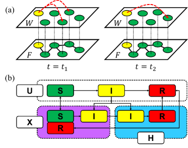
Figure 1: (a) The schematic diagram for the interaction on the DLMN. $W$ and $F$ layers are composed of the same set of nodes, i.e., the nodes at the ends of each dotted line are identical. The yellow infected node chooses random partners on $W$ at each time step $t=t_{1}$ and $t=t_{2}$ (red dashed arrows). Thus, on $W$ it interacts with different nodes at each $t$, while its interacting partner does not change on $F$ (black solid lines). (b) The change of states under the BIP or RIP. Red, yellow, and green boxes denote the states for $\sigma_{1}$, and white boxes represent the states for $\sigma_{2}$.

II.2 Intervention strategies

The state of each node at $t$ in the DLMN is described by a two-component variable ${\bm{\sigma}}=(\sigma_{1},\sigma_{2})$. $\sigma_{1}$ has one of the three disease states: $S$, $I$, and $R$. $\sigma_{2}$ denotes the state for isolation measure. Here, three isolation states are possible: i) self-isolation at home when an individual feels mild symptoms or recognizes a suspicious contact but has not been confirmed yet, and ii) hospitalization by the health authority when the patient is confirmed to be infected. If an individual is not isolated then it is in the iii) unisolated state. Thus, $\sigma_{2}$ can be one of the following states: self-isolated ($X$), hospitalized ($H$), and unisolated ($U$) (see Fig. 1 (b)).

Since we cannot trace the contacts on $W$ due to the random anonymity, the self-isolation for the suspicious contacts can be applied only to $F$. Depending on the range of the self-isolation, we introduce two intervention protocols, the basic isolation protocol (BIP) and the reinforced isolation protocol (RIP). Under the BIP only the confirmed patients and the one who has direct contact with the confirmed patient on $F$ are isolated. This is the most popular quarantine protocol adopted by many health authorities [35]. However, the fraction of the household or workplace infection cannot be ignored in some infectious diseases, for example, the household infection is more than 15% for COVID-19 [36]. Such household and workplace infection can be caused by a self-isolated individual. Furthermore, such transmissible paths can become a part of super-spreading events if the pre-symptomatic or asymptomatic infection is possible. Thus controlling such local contacts is another important factor to mitigate the transmission. For a preemptive protection of the susceptible, in the RIP model if a node is hospitalized, then its first and also second nearest neighbors on $F$ are isolated.

II.3 Basic isolation protocol

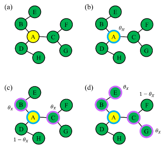
Figure 2: (a) On a network with size $N=8$ the node $A$ is infected while nodes $B\sim H$ are susceptible. (b) Node $A$ is hospitalized with probability $\theta_{H}$. (c) BIP and RIP: Node $B$ and $C$ are self-isolated with probability $\theta_{X}$ while node $D$ remains unisolated with probability $1-\theta_{X}$. (d) RIP: In addition to (c) node $E$ and $G$ are self-isolated with probability $\theta_{X}$ while node $F$ remains unisolated with probability $1-\theta_{X}$. Node $H$ are not included in the self-isolation candidate since node $D$ is not self-isolated in step (c).

In our models, each infected node transmits the disease to the connected susceptible nodes with the probability $\beta_{F}$ ($\beta_{W}$) on $F$ ($W$). With the probability $\theta_{X}$ ($\theta_{H}$) the nodes are self-isolated (hospitalized) for the isolation (hospitalization) period $t_{X}$ ($t_{H}$). The infected nodes are recovered after the recovery time $t_{R}$. To specify the update rule for each protocol, we introduce additional parameters $T_{i}^{I}$, $T_{i}^{X}$, and $T_{i}^{H}$ which denote the time of infection, self-isolation, and hospitalization for each node $i$, respectively.

In the BIP model, all nodes are initially in the state ${\bm{\sigma}}=(S,U)$. Then a node $i$ is randomly selected and set to be ${\bm{\sigma}}_{i}=(I,U)$ and $T^{I}_{i}=0$. At each time step $t$, three processes are repeated for all infected nodes whose time of infection is $T^{I}<t$: (1) infection, (2) isolation, and (3) unisolation and recovery. Each process is composed of the following sub-processes. Infection: (1-i) Each node $i$ with ${\bm{\sigma}}_{i}=(I,U)$ or $(I,X)$ transmits the disease to $k_{i}$ connected nodes on $F$ with the probability $\beta_{F}$ if the state of the connected node $j$ is ${\bm{\sigma}}_{j}=(S,U)$ or $(S,X)$. (1-ii) If $\sigma_{i,2}=U$, then it randomly chooses $k^{\prime}_{i}$ nodes on $W$ and infects with probability $\beta_{W}$ when the randomly chosen node $j$ is in the state ${\bm{\sigma}}_{j}=(S,U)$. $T^{I}_{j}$ for all new infected nodes $j$ is set to be $T^{I}_{j}=t$. Isolation: (2-i) Each infected node $i$ with $T^{I}_{i}<t$ is hospitalized with the probability $\theta_{H}$, i.e., $\sigma_{i,2}=H$ and $T^{H}_{i}=t$. (2-ii) Let $\Gamma_{i}$ be the set of nodes connected to the hospitalized node $i$ on $F$. Then we set $\sigma_{j,2}=X$ and $T^{X}_{j}=t$ for all $j\in\Gamma_{i}$ with the probability $\theta_{X}$, if $\sigma_{j,2}=U$ at $t-1$. This corresponds to the self-isolation. (2-iii) If the state of node $i$ was ${\bm{\sigma}}_{i}=(I,X)$ at $t-1$, then it becomes ${\bm{\sigma}}_{i}=(I,H)$ and $T^{H}_{i}=t$ for all $i(=1,2,\cdots,N)$. Unisolation and recovery: (3-i) For all nodes $i$ with $\sigma_{i,1}=I$ becomes $\sigma_{i,1}=R$, if $t>T^{I}_{i}+t_{R}$. Here $t_{R}$ is a constant representing a recovery time from the infection. (3-ii) For all nodes $i$ with $\sigma_{i,1}\in\left\{S,R\right\}$ and $\sigma_{i,2}=X$ are unisolated if $t>T_{i}^{X}+t_{X}$, where $t_{X}$ is the duration time for self-isolation. (3-iii) For all nodes $i$ with ${\bm{\sigma}}_{i}=(R,H)$, if $t>T^{H}_{i}+t_{H}$ then the node $i$ is released from hospitalization, and its state becomes ${\bm{\sigma}}_{i}=(R,U)$. Here $t_{H}$ denote the duration time for hospitalization. These processes are repeated until there left no infected node. Under the BIP only the confirmed patients and the one who has direct contact with the confirmed patient are isolated as shown in Fig. 2. This is the most popular quarantine protocol adopted by many health authorities over the globe [35].

II.4 Reinforced isolation protocol

The RIP can be implemented by adding the sub-process (2-iv) to the end of the isolation process of the BIP: (2-iv) Let $j$ be the node whose state is changed into $\sigma_{j,2}=X$ at $t$ and $\Gamma_{j}$ be the set of nodes connected to $j$ on $F$. Then the state of node $n(\in\Gamma_{j})$ with $\sigma_{n,2}=U$ also becomes $\sigma_{n,2}=X$ with the same probability $\theta_{X}$ for all $n$. Thus, in the RIP model if a node is hospitalized, then its first and second nearest neighbors on $F$ are isolated with the given probability (see Fig. 2).

In the following simulations, we set the size of each layer as $N=100,000$ and use the mean degrees $\left<k\right>=\left<k^{\prime}\right>=8$. The value of the mean degree only affects the epidemic threshold [31], and does not change the main conclusion. The epidemic threshold of susceptible-infected-recovered (SIR) model is related to percolation threshold and the branching factor [31, 22, 24, 37]. Since we are interested in the control of the severe epidemic outbreak, we use $\beta_{F}=\beta_{W}\equiv\beta(=0.2)$ and $t_{R}=6$ to guarantee that the whole system becomes infected without any intervention (see Appendix A). In our model, the strength of the intervention measures is controlled by four parameters, $\theta_{H}$, $t_{H}$, $\theta_{X}$, and $t_{X}$. For simplicity, we assume that $\theta_{H}=\theta_{X}\equiv\theta^{*}$ and $t_{H}=t_{X}\equiv t^{*}$. Thus, we use only two control parameters $\theta^{*}$ and $t^{*}$.

III Results

III.1 The fraction of nodes in each state

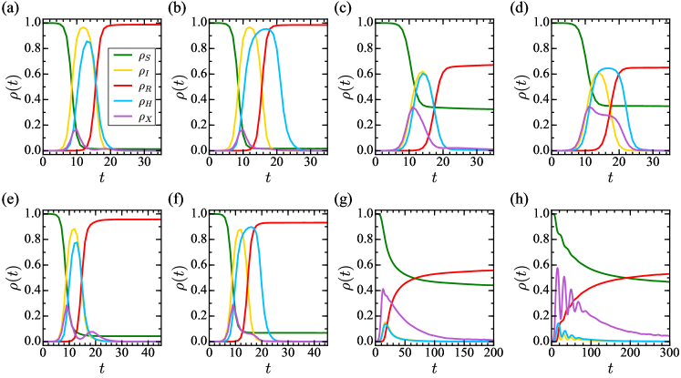
Figure 3: (a)-(d) are {$\rho_{m}(t)$}’s ($m\in\left\{S,I,R,H,X\right\}$) under the BIP with (a) $\theta^{*}=0.3$, $t^{*}=4$, (b) $\theta^{*}=0.3$, $t^{*}=10$, (c) $\theta^{*}=0.9$, $t^{*}=4$, (d) $\theta^{*}=0.9$, $t^{*}=10$. (e)-(h) show {$\rho_{m}(t)$}’s under the RIP with (e) $\theta^{*}=0.3$, $t^{*}=4$, (f) $\theta^{*}=0.3$, $t^{*}=10$, (g) $\theta^{*}=0.9$, $t^{*}=4$, (h) $\theta^{*}=0.9$, $t^{*}=10$. $\beta=0.2$ and $t_{R}=6$ are used in common. Each data is obtained from 500 independent simulations by averaging the surviving samples at time $t$.

Let $\rho_{m}(t)$ ($m\in\{S,I,R\}$) be the fraction of nodes whose disease states is $\sigma_{1}=m$ at time $t$, regardless of $\sigma_{2}$. If $m\in\{U,H,X\}$, then $\rho_{m}(t)$ represents the fraction of nodes with $\sigma_{2}=m$. The peak of $\rho_{m}(t)$ for each state $m$ is denoted by $\rho^{peak}_{m}$. In Figs. 3 (a)-(d) we show $\{\rho_{m}(t)\}$’s under the BIP for various values of parameters $(\theta^{*},t^{*})$. For small $\theta^{*}(=0.3)$, we find that $\rho^{peak}_{I}(t)>0.9$ followed by $\rho^{peak}_{H}(\gtrsim 0.8)$, regardless of $t^{*}$ (Figs. 3 (a), (b)). $\rho_{S}(t)$ rapidly decreases and reaches $\rho_{S}\approx 0$ for $t>11$. The value of $\rho^{peak}_{X}$ ($<0.2$) is relatively small. Thus, $\rho_{R}(t\rightarrow\infty)\simeq 1$ when $\theta^{*}$ is small. On the other hand, as $\theta^{*}$ increases, $\rho^{peak}_{I}$ is drastically suppressed as well as $\rho^{peak}_{H}$ (Figs. 3 (c), (d)). As a result, $\rho_{R}(t\rightarrow\infty)$ is reduced to $\rho_{R}(t\rightarrow\infty)\simeq 0.6\sim 0.7$ for $\theta^{*}=0.9$. For both values of $\theta^{*}$ displayed in Figs. 3, $t^{*}$ only affects the behavior of $\rho_{H}$ and $\rho_{X}$ (the population of the isolated nodes). Note that $\rho^{peak}_{H}$ is comparable with $\rho^{peak}_{I}$ for all values of $(\theta^{*},t^{*})$, and $\rho_{H}(t)$ becomes wider as $t^{*}$ increases. This means that the hospitalized period becomes longer without any significant change in the final epidemic size, $\rho_{R}(t\rightarrow\infty)$, as $t^{*}$ increases for all $\theta^{*}$. Thus, increasing $t^{*}$ without the improvement of traceability causes an overload on the medical system by making patients be hospitalized for a longer period.

Figs. 3 (e)-(h) show $\{\rho_{m}(t)\}$’s for the RIP model. When $\theta^{*}\lesssim 0.3$, $\{\rho_{m}(t)\}$’s for the RIP model show almost the similar behavior with those for the BIP, but $\rho_{S}(t\rightarrow\infty)$ for the RIP is slightly larger than that for the BIP. Since additional nodes are self-isolated under the RIP, $\rho_{X}^{peak}$ increases compared with that for the BIP with the same $(\theta^{*}$, $t^{*}$). However, we find that $\rho_{H}$ for the RIP becomes much smaller than that for the BIP. This effect becomes more drastic for $\theta^{*}>0.3$. For example, $\rho_{R}(t\rightarrow\infty)$ and $\rho_{I}^{peak}(t)$ significantly decrease to $\rho_{R}(t\rightarrow\infty)=0.5\sim 0.6$ and $\rho_{I}^{peak}\approx 0.1$ for the RIP with $\theta^{*}=0.9$. The results indicate that the collapse of the medical systems can be avoided under the RIP if we trace the contacts with sufficiently high accuracy. In addition, we find $\rho_{I}$, $\rho_{H}$, and $\rho_{X}$ oscillate with decreasing amplitude under the RIP as $\theta^{*}$ increases. This suggests that even though there is a rapid decrease in $\rho_{I}(t)$ after its first peak when $\theta^{*}$ is sufficiently large, it is still possible to be followed by successive multiple peaks of $\rho_{I}$. See Appendix B for a more detailed description on this oscillatory behavior. For comparison, we also display the evolution of $\left\{\rho_{m}(t)\right\}$’s when $P_{F}(k)\sim k^{-\gamma}$ in Appendix C.1.

III.2 The effective reproduction number

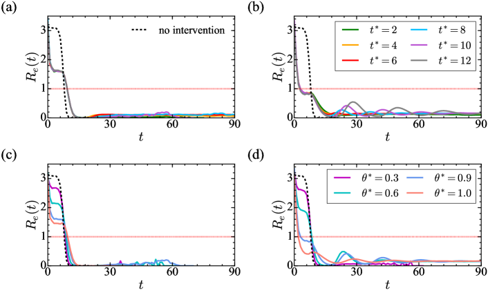
Figure 4: Plot of $R_{e}(t)$ under the (a) BIP and (b) RIP when $t^{*}=2\sim 12$ and $\theta^{*}=0.9$ with $\beta=0.2$, $t_{R}=6$. Plot of $R_{e}(t)$ for the (c) BIP and (d) RIP when $t^{*}=10$ and $\theta^{*}=0,3\sim 1.0$ with $\beta=0.2$, $t_{R}=6$. The black dashed curve denotes the case when the isolation protocol is absent. The red dotted horizontal line depicts $R_{e}(t)=1$.

To quantify the efficacy of intervention measures, we estimate the instantaneous effective reproduction number, $R_{e}(t)$, at $t$. For a practical purpose, we define $R_{e}(t)$ as

$$R_{e}(t)=\frac{N^{new}_{I}(t)}{N_{I}(t-1)},$$ (1)

where $N^{new}_{I}(t)$ is the number of new infected nodes at $t$ and $N_{I}(t)$ is the number of infected nodes at $t$ [38, 39]. Thus $R_{e}(t)$ represents a metric to quantify how many nodes are newly infected by the existing infected nodes at each $t$.

In Figs. 4 (a) and (b), we show $R_{e}(t)$ for the BIP and RIP with $\theta^{*}=0.9$ and $t^{*}=2\sim 12$. The dashed line denotes $R_{e}(t)$ without intervention. As shown in Fig. 4 (a), $R_{e}(t)$ for the BIP rapidly decreases when $t\lesssim 4$ and shows a plateau followed by another rapid drop, regardless of $t^{*}$. $R_{e}(t)=1$ at $t\approx 11$ and $R_{e}(t)<1$ for $t>11$. When $t>15$ $R_{e}(t)$ approaches to $R_{e}(t)\approx 0$. On the other hand, $R_{e}(t)$ for $\theta^{*}=0.9$ under the RIP decreases more drastically and $R_{e}(t)<1$ for $t\gtrsim 5$ as shown in Fig. 4 (b). When $t>20$, $R_{e}(t)$ oscillates with decreasing amplitudes and approaches $R_{e}\approx 0$ under the RIP.

To investigate how $\theta^{*}$ affects the epidemic spreading, we also measure $R_{e}(t)$’s for various $\theta^{*}$ when $t^{*}$ is fixed. In Figs. 4 (c) and (d), as an example, we display $R_{e}(t)$’s for $t^{*}=10$. Since $\theta^{*}$ denotes traceability, $R_{e}(t)$ should decrease as $\theta^{*}$ increases for both protocols as shown in Figs. 4 (c) and (d). Note that when $\theta^{*}<0.3$, the difference between the BIP and RIP is not noticeable. However, if $\theta^{*}>0.3$, then $R_{e}(t)$ for the RIP becomes much smaller than those for the BIP. From the data in Fig. 4, we find that increasing $\theta^{*}$ is more important than increasing $t^{*}$.

The rapid drop of $R_{e}(t)$ under both protocols has two different origins depending on $\theta^{*}$. For $\theta^{*}<0.3$ due to the large infection of the early stage, there does not remain a sufficient number of susceptible nodes for $t>11$ (see Figs. 3 (a), (b), (e), (f)). On the other hand, if $\theta^{*}>0.3$ then a significant amount of the susceptible is self-isolated, which protects the susceptible nodes before contact with the patients for $t>10$ (see Figs. 3 (c), (d), (g), (h)).

III.3 The final epidemic size

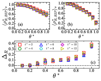
Figure 5: We plot the average final epidemic size under the (a) BIP and (b) RIP for $t^{*}=2\sim 12$ and $\theta^{*}=0.1\sim 1.0$. The increment of the isolation period ($t^{*}$) has negligible effect on the final epidemic size while the traceability ($\theta^{*}$) significantly changes the final epidemic size. (c) We plot the difference of the final epidemic sizes between the BIP and RIP, $\Delta_{R}$. The black horizontal dashed line denotes $\Delta_{R}=0$.

In order to evaluate the effectiveness of the isolation protocols, we obtained the final epidemic size. The final epidemic size under each protocol $Y$($=BIP$ or $RIP$) is defined as $\rho^{*}_{R,Y}\equiv\rho_{R,Y}(t\rightarrow\infty)$. In Figs. 5 (a) and (b), we plot $\left<\rho_{R,BIP}^{*}\right>_{s}$ and $\left<\rho_{R,RIP}^{*}\right>_{s}$ with various parameter sets, $(\theta^{*},t^{*})$. Here $\left<...\right>_{s}$ denotes the sample average over independent runs. We used $10,000$ samples to obtain the average final epidemic size. The results show that $t^{*}$ has a negligible effect on the final epidemic size. This suggests that extending the isolation period will simply add a burden on the socio-economic system unless there is any improvement in the ability to trace the infection routes.

For a direct comparison between the two intervention protocols, we measure the difference of the final epidemic sizes between the BIP and RIP, $\Delta_{R}(t^{*},\theta^{*})$, for each $t^{*}$ and $\theta^{*}$. $\Delta_{R}(t^{*},\theta^{*})$ is defined as

$$\Delta_{R}(t^{*},\theta^{*})\equiv\left<\rho_{R,BIP}^{*}(t^{*},\theta^{*})\right>_{s}-\left<\rho_{R,RIP}^{*}(t^{*},\theta^{*})\right>_{s}.$$ (2)

Thus, if $\Delta_{R}>0$ then $\rho_{R}$ for the BIP is larger than that for the RIP. The data in Fig. 5 (c) clearly shows that $\Delta_{R}$ rarely depends on $t^{*}$. However, $\Delta_{R}$ strongly depends on $\theta^{*}$. $\Delta_{R}\leq 0.05$ for all $t^{*}$ when $\theta^{*}<0.3$, while $\Delta_{R}>0.1$ for $\theta^{*}\gtrsim 0.4$ and $\Delta_{R}$ increases as $\theta^{*}$ increases. This means that the RIP significantly reduces the final epidemic size compared to the BIP when $\theta^{*}\geq 0.3$. For the maximal traceability, $\theta^{*}=1$, we find that $\rho_{R}(t\rightarrow\infty)$ for the RIP is reduced by 67% compared to that for the BIP. This corresponds to the 100% increase of $\rho_{S}(t\rightarrow\infty)$ under the RIP compared to the BIP. Thus, isolation of the possible suspicious contacts in advance by applying the RIP significantly reduces the final epidemic size when $\theta^{*}\geq 0.3$.

III.4 The number of isolated nodes per unit time

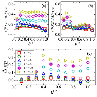
Figure 6: We plot the average fraction of the isolated nodes per unit time under the (a) BIP and (b) RIP for $t^{*}=2\sim 12$ and $\theta^{*}=0.1\sim 1.0$. Under the BIP, $\left<\left<\rho_{XH,BIP}\right>_{t}\right>_{s}$ hardly change as $\theta^{*}$ increases for a fixed $t^{*}$. However, when the RIP is applied, $\left<\left<\rho_{XH,RIP}\right>_{t}\right>_{s}$ drastically decrease when $\theta^{*}>0.3$. and $t^{*}>6$. This suggests that with high traceability, the RIP can effectively mitigate the epidemic spreading while minimizing the damage on the social and economic system.

In epidemic control, reducing the number of isolated individuals at each time step becomes another crucial factor to minimize social and economic recession. Here, we define the fractions of the isolated nodes per unit time (with $\sigma_{2}=X$ or $H$) for protocol $Y$ as,

$$\left<\rho_{XH,Y}\right>_{t}=\frac{\int_{0}^{T_{final}}(\rho_{X}(t)+\rho_{H}(t))dt}{T_{final}},$$ (3)

where $T_{final}$ represents the time at which $\rho_{I}(t)$ becomes zero. In Figs. 6 (a) and (b), we plot $\left<\left<\rho_{XH,BIP}\right>_{t}\right>_{s}$ and $\left<\left<\rho_{XH,RIP}\right>_{t}\right>_{s}$, where $\left<...\right>_{s}$ denotes the sample average over independent samples. The sample averages are obtained from 500 independent trajectories. The data in Fig. 6 (a) shows that $\left<\left<\rho_{XH,BIP}\right>_{t}\right>_{s}$ hardly changes as $\theta^{*}$ increases except for $\theta^{*}=0.1$. Moreover, longer isolation period leads to a larger values of $\left<\left<\rho_{XH,BIP}\right>_{t}\right>_{s}$ in general. However, when the RIP is adopted, there is a significant drop in $\left<\left<\rho_{XH,RIP}\right>_{t}\right>_{s}$ when $\theta^{*}>0.3$ and $t^{*}>6$.

For a quantitative analysis, we define the difference in the fractions of the isolated nodes per unit time between two protocols as

$$\Delta_{XH}\equiv\left<\left<\rho_{XH,BIP}\right>_{t}\right>_{s}-\left<\left<\rho_{XH,RIP}\right>_{t}\right>_{s}.$$ (4)

By definition, if $\Delta_{XH}>0$ then more nodes are isolated under the BIP than the RIP. As shown in Fig. 6 (c), for all values of $\theta^{*}$, we find that $\Delta_{XH}\approx 0$ for $t^{*}\leq 6$. However, we find that $\Delta_{XH}>0$ when $t^{*}>6$ and $\Delta_{XH}$ increases as $t^{*}$ increases. Thus, $t^{*}$ affects only $\rho_{X}$ and $\rho_{H}$ per unit time for both models. Note that, even though $\Delta_{XH}\leq 0$ for $t^{*}\leq 6$, $\Delta_{R}$ increases with $\theta^{*}$ and $\Delta_{R}\geq 0$ as shown in Fig. 5 (c) (see also Fig. 3). Therefore, the RIP more effectively controls the disease spreading through the preemptive isolation of suspicious contacts with fewer isolated nodes per unit time than the BIP. We also display the measured $\Delta_{R}$ and $\Delta_{XH}$ when $P_{F}(k)\sim k^{-\gamma}$ in Appendix C.2, which are almost identical with those in Figs. 5 and 6.

IV Discussion

In summary, we model the NPI adopted by many health authorities over the world, and introduce a model for reinforced NPI. In these models the state of each individual is characterized by three disease states with additional isolation states. Two different types of transmission routes observed in real world are implemented by the multiplex networks. By using numerical simulations, we compare the efficacy of the two models, BIP and RIP models, and find that the RIP controls the spreading of disease more efficiently by reducing both the epidemic size and the average number of isolated individuals per unit time, despite its simplicity. Especially, when the traceability is maximal, the final fraction of the susceptible nodes under the RIP increases by almost 100% (almost doubled) compared to that under the BIP. This indicates that the RIP significantly and efficiently protect the susceptible nodes through the preemptive isolation of the possible contacts. Furthermore, since we do not assume any characteristic property of a specific disease, we expect that the suggested models can be used as a general framework for modeling disease control for any real disease outbreak.

Appendix A Epidemic Threshold on DLMN

A.1 Estimating $\beta_{c}$

To estimate $\beta_{c}$ we first define the transmissibility $\mathcal{T}$. When a node $j$ is infected at time $t=t_{0}$, a susceptible neighbor $i$ can be infected by $j$ at time $t=t_{0}+n$ with the probability $\beta(1-\beta)^{n-1}$ where $n=1,2,...,t_{R}$. By adding up the probabilities for all possible values of $n$, we can get $\mathcal{T}$ as [37]

$$\mathcal{T}=\sum_{n=1}^{t_{R}}\beta(1-\beta)^{n-1}=1-(1-\beta)^{t_{R}}.$$ (5)

The transition between the disease-free phase and the epidemic phase is determined by the average number of the secondary infections per infected node. The average number of the secondary neighbor is

$$\sum_{k}k\frac{kP(k)}{\left<k\right>}-1=\frac{\left<k^{2}\right>-\left<k\right>}{\left<k\right>}=\kappa-1,$$ (6)

where $\kappa\equiv\left<k^{2}\right>/\left<k\right>$ is known as the branching factor. Thus, when $\mathcal{T}(\kappa-1)\geq 1$, the epidemic spreads out over the network (epidemic phase). However, when $\mathcal{T}(\kappa-1)<1$, the disease dies out in a short time scale (disease-free phase) [37]. Therefore, the critical transmissibility $\mathcal{T}_{c}$ is given by

$$\mathcal{T}_{c}=\frac{1}{\kappa-1}=\frac{\left<k\right>}{\left<k^{2}\right>-\left<k\right>}.$$ (7)

From Eqs. (5) and (7), $\beta_{c}$ is determined by the relation

$$1-(1-\beta_{c})^{t_{R}}=\frac{\left<k\right>}{\left<k^{2}\right>-\left<k\right>}.$$ (8)

A.2 $\left<k\right>$ and $\left<k^{2}\right>$ of DLMN

Let $G_{F}(x)$ and $G_{W}(x)$ be the generating functions of $P_{F}(k)$ and $P_{W}(k)$, respectively, which are defined by

$$G_{F}(x)=\sum_{k=0}^{\infty}P_{F}(k)x^{k}$$ (9)

and

$$G_{W}(x)=\sum_{k=0}^{\infty}P_{W}(k)x^{k}.$$ (10)

Then the combined degree distribution of both layers becomes

$$P(k^{\prime})=\sum_{k_{1}=1}^{\infty}\sum_{k_{2}=1}^{\infty}\delta(k^{\prime},k_{1}+k_{2})P_{F}(k_{1})P_{W}(k_{2}).$$ (11)

Here $\delta(i,j)$ is Kronecker’s delta. The generating function of $P(k^{\prime})$, $G(x)$, is simply written as

$$G(x)=G_{F}(x)G_{W}(x).$$ (12)

On DLMN due to the time-dependent feature of degree on the $W$-layer, $P_{W}(k)$ is well approximated by the Poisson distribution, $P_{W}(k)=\left<k\right>^{-k}\exp(-\left<k\right>)/k!$. When $P_{F}(k)$ is given by $P_{F}(k)=\left<k\right>^{-k}\exp(-\left<k\right>)/k!$, from Eq. 9, 10 and 12, we obtain

$$G(x)=\exp\left\{2\left<k\right>(x-1)\right\},$$ (13)

and $\left<k^{\prime}\right>=2\left<k\right>$ and $\left<{k^{\prime}}^{2}\right>=2\left<k\right>+(2\left<k\right>)^{2}$. Thus, we numerically estimate the threshold from Eq. (8) as $\beta_{c}\approx 0.0107$.

On the other hand, when $P_{F}(k)=k^{-\gamma}/\zeta(\gamma)$ and $P_{W}(k)=\left<k\right>^{-k}\exp(-\left<k\right>)/k!$, we obtain $\left<k^{\prime}\right>=(\left<k\right>\mathrm{Li}_{\gamma}(1)+\mathrm{Li}_{\gamma-1}(1))/\zeta(\gamma)$ and $\left<{k^{\prime}}^{2}\right>=\left[\left<k\right>(\left<k\right>+1)\mathrm{Li}_{\gamma}(1)+2\left<k\right>\mathrm{Li}_{\gamma-1}(1)+\mathrm{Li}_{\gamma-2}(1)\right]/\zeta(\gamma)$. Here $\zeta(\gamma)$ is the Riemman zeta function and $\mathrm{Li}_{\gamma}(x)$ is the polylogarithm of $x$. Thus, $\beta_{c}=0$ for $2<\gamma<3$.

Therefore, $\beta=0.2$ guarantees that the the system is in the epidemic phase, regardless of the structure of $F$-layer with given parameters.

Appendix B Oscillatory Behavior

Under the RIP with large values of $\theta^{*}$ and $t^{*}$, oscillatory behaviors are observed in the fraction of nodes in each sate when $P_{F}(k)$ follows the Poisson distribution. In Fig. 7, we plot $\rho_{H}$, $\rho_{I}$ and $\rho_{f}$ which clearly shows such oscillatory behaviors. Here, $\rho_{f}(t)$ is defined as the fraction of the susceptible nodes which are just released from self-isolation at time $t$. We used the intervention parameters as $\theta^{*}=0.9$ and $t^{*}=12$. The period of oscillation $\tau$ for each fraction with the given parameters is estimated as $\tau\approx 21$. The peak position of each curve indicates that the increase of the infected causes an increase of the hospitalized individuals. Due to the hospitalization and self-isolation, the number of the infected rapidly decreases. However, after $t^{*}$ the isolated nodes are set to be free which increases the number of unisolated susceptible nodes. Thus it increases the number of infected individuals again. This pattern is repeated with decreasing amplitude due to the depletion of the susceptible nodes until there is no more infected node left. This oscillatory behavior is observed only for the case of large $\theta^{*}$ and $t^{*}$ in the RIP.

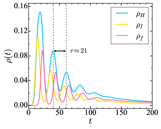
Figure 7: Plot of the fractions $\rho_{H}$, $\rho_{I}$ and $\rho_{f}$ under the RIP. The epidemic parameters are $\beta=0.2$ and $t_{R}=6$, and the intervention parameters are $\theta^{*}=0.9$ and $t^{*}=12$.

Appendix C Results when $P_{F}(k)\sim k^{-\gamma}$

In this section we summarize the obtained results when $P_{F}(k)$ follows the power-law, $P_{F}(k)\sim k^{-\gamma}$, with degree exponent $\gamma=2.7$. For a direct comparison with the results in the main text, we set $\left<k\right>=8$ and $N=100,000$. We use the static model [40] to construct the $F$-layer with a power-law degree distribution. Except the underlying topology of $F$-layer, other parameters are the same with those in the main text.

C.1 Evolution of $\left\{\rho_{m}(t)\right\}$’s

The data in Fig. 8 shows $\left\{\rho_{m}(t)\right\}$’s when $P_{F}(k)\sim k^{-\gamma}$. As shown in Fig. 8, the qualitative behavior of $\left\{\rho_{m}(t)\right\}$’s are almost the same with those in Fig. 3. The only difference is the decrease of $\rho_{R}$ when $\theta^{*}$ is large (see Figs. 8(g) and (h)). Since the average number of the secondary neighbors on $F$-layer becomes large if $P_{F}(k)$ follows the power-law, more nodes are in the $X$ state compared with the Poisson distribution case. This effect becomes larger as $\theta^{*}$ increases. Thus, more nodes are isolated and protected from the infection. As a result, the $\rho_{S}$ increase when $P_{F}(k)\sim k^{-\gamma}$ as shown in Figs. 8(g) and (h).

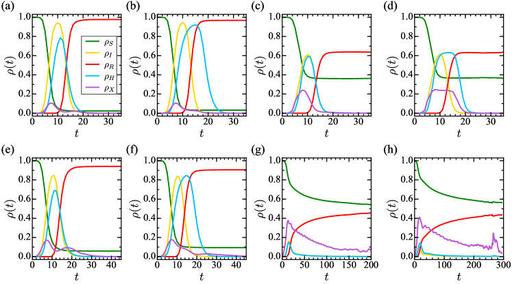
Figure 8: (a)-(d) are {$\rho_{m}(t)$}’s ($m\in\left\{S,I,R,H,X\right\}$) under the BIP when $P_{F}(k)\sim k^{-\gamma}$ with (a) $\theta^{*}=0.3$, $t^{*}=4$, (b) $\theta^{*}=0.3$, $t^{*}=10$, (c) $\theta^{*}=0.9$, $t^{*}=4$, (d) $\theta^{*}=0.9$, $t^{*}=10$. (e)-(h) shows {$\rho_{m}(t)$}’s under the RIP with (e) $\theta^{*}=0.3$, $t^{*}=4$, (f) $\theta^{*}=0.3$, $t^{*}=10$, (g) $\theta^{*}=0.9$, $t^{*}=4$, (h) $\theta^{*}=0.9$, $t^{*}=10$. $\beta=0.2$ and $t_{R}=6$ are used in common. Each data is obtained from 500 independent simulations by averaging the surviving samples at time $t$.

C.2 Final epidemic size and the number of isolated nodes per unit time

In Fig. 9 we also display the measured difference of the final epidemic sizes and the numbers of isolated nodes between the BIP and RIP for various values of $\theta^{*}$. As shown in the data, we find that the underlying topology of $F$-layer hardly affect the behavior of final epidemic size and number of isolated nodes. The obtained data are qualitatively the same with those in Figs.5 (c) and 6 (c).

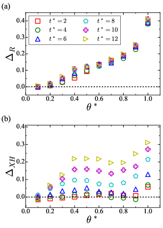
Figure 9: We plot (a) the difference of the final epidemic sizes between the BIP and RIP, $\Delta_{R}$ and (b) the difference of the numbers of isolated nodes per unit time between the BIP and RIP, $\Delta_{XH}$ when $P_{F}(k)\sim k^{-\gamma}$. The black horizontal dashed line denotes $\Delta_{R}=0$.

References

- Gould [1966] G. M. Gould, Anomalies and curiosities of medicine (Blacksleet River, 1966).
- Taubenberger and Morens [2006] J. K. Taubenberger and D. M. Morens, 1918 Influenza: the mother of all pandemics, Revista Biomedica 17, 69 (2006).
- Chan-Yeung and Xu [2003] M. Chan-Yeung and R.-H. Xu, SARS: epidemiology, Respirology 8, S9 (2003).
- WHO [2020] WHO, WHO COVID-19 dashboard, https://covid19.who.int/. (2020).
- Ren [2020] X. Ren, Pandemic and lockdown: a territorial approach to COVID-19 in China, Italy and the United States, Eurasian Geography and Economics 61, 423 (2020).
- Lu et al. [2021] G. Lu, O. Razum, A. Jahn, Y. Zhang, B. Sutton, D. Sridhar, K. Ariyoshi, L. von Seidlein, and O. Müller, COVID-19 in Germany and China: mitigation versus elimination strategy, Global health action 14, 1875601 (2021).
- Harvey [2020] N. Harvey, Behavioral fatigue: real phenomenon, naïve construct, or policy contrivance?, Frontiers in Psychology 11, 2960 (2020).
- Nicola et al. [2020] M. Nicola, Z. Alsafi, C. Sohrabi, A. Kerwan, A. Al-Jabir, C. Iosifidis, M. Agha, and R. Agha, The socio-economic implications of the coronavirus pandemic (COVID-19): A review, International journal of surgery 78, 185 (2020).
- Ferretti et al. [2020] L. Ferretti, C. Wymant, M. Kendall, L. Zhao, A. Nurtay, L. Abeler-Dörner, M. Parker, D. Bonsall, and C. Fraser, Quantifying SARS-CoV-2 transmission suggests epidemic control with digital contact tracing, Science 368 (2020).
- Flaxman et al. [2020] S. Flaxman, S. Mishra, A. Gandy, H. J. T. Unwin, T. A. Mellan, H. Coupland, C. Whittaker, H. Zhu, T. Berah, J. W. Eaton, et al., Estimating the effects of non-pharmaceutical interventions on COVID-19 in Europe, Nature 584, 257 (2020).
- Perra [2021] N. Perra, Non-pharmaceutical interventions during the COVID-19 pandemic: A review, Physics Reports 913 (2021).
- Maier and Brockmann [2020] B. F. Maier and D. Brockmann, Effective containment explains subexponential growth in recent confirmed COVID-19 cases in China, Science 368, 742 (2020).
- Chan et al. [2021] L. Y. H. Chan, B. Yuan, and M. Convertino, COVID-19 non-pharmaceutical intervention portfolio effectiveness and risk communication predominance, Scientific Reports 11, 1 (2021).
- Thurner et al. [2020] S. Thurner, P. Klimek, and R. Hanel, A network-based explanation of why most COVID-19 infection curves are linear, Proceedings of the National Academy of Sciences 117, 22684 (2020).
- Nimmagadda et al. [2020] V. Nimmagadda, O. Kogan, and E. Khain, Path-dependent course of epidemic: Are two phases of quarantine better than one?, Europhysics Letters 132, 28003 (2020).
- Mukhamadiarov et al. [2021] R. I. Mukhamadiarov, S. Deng, S. R. Serrao, Priyanka, R. Nandi, L. H. Yao, and U. C. Täuber, Social distancing and epidemic resurgence in agent-based Susceptible-Infectious-Recovered models, Scientific Reports 11, 1 (2021).
- Choi et al. [2020] K. Choi, H. Choi, and B. Kahng, Covid-19 epidemic under the K-quarantine model: Network approach (2020), arXiv:2010.07157 .
- Arenas et al. [2020] A. Arenas, W. Cota, J. Gómez-Gardeñes, S. Gómez, C. Granell, J. T. Matamalas, D. Soriano-Paños, and B. Steinegger, Modeling the spatiotemporal epidemic spreading of COVID-19 and the impact of mobility and social distancing interventions, Physical Review X 10, 041055 (2020).
- Schlosser et al. [2020] F. Schlosser, B. F. Maier, O. Jack, D. Hinrichs, A. Zachariae, and D. Brockmann, COVID-19 lockdown induces disease-mitigating structural changes in mobility networks, Proceedings of the National Academy of Sciences 117, 32883 (2020).
- Sneppen et al. [2021] K. Sneppen, B. F. Nielsen, R. J. Taylor, and L. Simonsen, Overdispersion in COVID-19 increases the effectiveness of limiting nonrepetitive contacts for transmission control, Proceedings of the National Academy of Sciences 118 (2021).
- Pastor-Satorras and Vespignani [2001] R. Pastor-Satorras and A. Vespignani, Epidemic dynamics and endemic states in complex networks, Physical Review E 63, 066117 (2001).
- Newman [2002] M. E. J. Newman, Spread of epidemic disease on networks, Physical Review E 66, 016128 (2002).
- Balcan et al. [2009] D. Balcan, V. Colizza, B. Gonçalves, H. Hu, J. J. Ramasco, and A. Vespignani, Multiscale mobility networks and the spatial spreading of infectious diseases, Proceedings of the National Academy of Sciences 106, 21484 (2009).
- Zuzek et al. [2015] L. G. A. Zuzek, H. E. Stanley, and L. A. Braunstein, Epidemic model with isolation in multilayer networks, Scientific Reports 5, 1 (2015).
- Parmet and Sinha [2020] W. E. Parmet and M. S. Sinha, Covid-19—the law and limits of quarantine, New England Journal of Medicine 382, e28 (2020).
- Fraser et al. [2004] C. Fraser, S. Riley, R. M. Anderson, and N. M. Ferguson, Factors that make an infectious disease outbreak controllable, Proceedings of the National Academy of Sciences 101, 6146 (2004).
- Peak et al. [2017] C. M. Peak, L. M. Childs, Y. H. Grad, and C. O. Buckee, Comparing nonpharmaceutical interventions for containing emerging epidemics, Proceedings of the National Academy of Sciences 114, 4023 (2017).
- Tong et al. [2020] Z.-D. Tong, A. Tang, K.-F. Li, P. Li, H.-L. Wang, J.-P. Yi, Y.-L. Zhang, and J.-B. Yan, Potential presymptomatic transmission of SARS-CoV-2, Zhejiang province, China, 2020, Emerging infectious diseases 26, 1052 (2020).
- Bai et al. [2020] Y. Bai, L. Yao, T. Wei, F. Tian, D.-Y. Jin, L. Chen, and M. Wang, Presumed asymptomatic carrier transmission of COVID-19, JAMA 323, 1406 (2020).
- Zhang et al. [2020] R. Zhang, Y. Li, A. L. Zhang, Y. Wang, and M. J. Molina, Identifying airborne transmission as the dominant route for the spread of COVID-19, Proceedings of the National Academy of Sciences 117, 14857 (2020).
- Newman [2018] M. E. J. Newman, Networks, 2nd ed. (Oxford university press, 2018).
- Hethcote [2000] H. W. Hethcote, The mathematics of infectious diseases, SIAM review 42, 599 (2000).
- Solomonoff and Rapoport [1951] R. Solomonoff and A. Rapoport, Connectivity of random nets, The bulletin of mathematical biophysics 13, 107 (1951).
- Erdős and Rényi [1960] P. Erdős and A. Rényi, On the evolution of random graphs, Publications of the Mathematical Institute of the Hungarian Academy of Science 5, 17 (1960).
- Webster et al. [2020] R. K. Webster, S. K. Brooks, L. E. Smith, L. Woodland, S. Wessely, and G. J. Rubin, How to improve adherence with quarantine: rapid review of the evidence, Public Health 182, 163 (2020).
- Park et al. [2020] Y. J. Park, Y. J. Choe, O. Park, S. Y. Park, Y.-M. Kim, J. Kim, S. Kweon, Y. Woo, J. Gwack, S. S. Kim, et al., Contact tracing during coronavirus disease outbreak, South Korea, 2020, Emerging infectious diseases 26, 2465 (2020).
- Lagorio et al. [2011] C. Lagorio, M. Dickison, F. Vazquez, L. A. Braunstein, P. A. Macri, M. V. Migueles, S. Havlin, and H. E. Stanley, Quarantine-generated phase transition in epidemic spreading, Physical Review E 83, 026102 (2011).
- Fraser [2007] C. Fraser, Estimating individual and household reproduction numbers in an emerging epidemic, PloS one 2, e758 (2007).
- Cori et al. [2013] A. Cori, N. M. Ferguson, C. Fraser, and S. Cauchemez, A new framework and software to estimate time-varying reproduction numbers during epidemics, American journal of epidemiology 178, 1505 (2013).
- Goh et al. [2001] K.-I. Goh, B. Kahng, and D. Kim, Universal behavior of load distribution in scale-free networks, Physical Review Letters 87, 278701 (2001).