Non-Hermitian topology in rock-paper-scissors games

Abstract

Abstract Non-Hermitian topology is a recent hot topic in condensed matters. In this paper, we propose a novel platform drawing interdisciplinary attention: rock-paper-scissors (RPS) cycles described by the evolutionary game theory. Specifically, we demonstrate the emergence of an exceptional point and a skin effect by analyzing topological properties of their payoff matrix. Furthermore, we discover striking dynamical properties in an RPS chain: the directive propagation of the population density in the bulk and the enhancement of the population density only around the right edge. Our results open new avenues of the non-Hermitian topology and the evolutionary game theory.

Introduction
In these decades, the notion of the topology has played a central role in condensed matter physics Kane & Mele (2005); Bernevig et al. (2006); König et al. (2007); Hasan & Kane (2010); Qi & Zhang (2011). Analysis of topological aspects of condensed matters dates back to integer quantum Hall systems Klitzing et al. (1980) which exhibit robust chiral edge modes induced by the topology of the Hermitian Hamiltonian in the bulk Thouless et al. (1982); Halperin (1982); Hatsugai (1993). While these robust edge modes are originally reported for quantum systems, they have been extended to various disciplines of science Haldane & Raghu (2008); Wang et al. (2009); Fu et al. (2010); Ozawa et al. (2019); Prodan & Prodan (2009); Kane & Lubensky (2013); Kariyado & Hatsugai (2015); Süsstrunk & Huber (2015); Delplace et al. (2017); Sone & Ashida (2019); Yoshida & Hatsugai (2021). In particular, the notion of topology has been extended to an interdisciplinary field Knebel et al. (2020); Yoshida et al. (2021); the emergence of topological edge modes has been predicted Yoshida et al. (2021) for networks of rock-paper-scissors (RPS) cycles which are described by the evolutionary game theory Weibull (1997); Sigmund (2011); Kirkup & Riley (2004); Rosas (2010); Wang et al. (2013); Perc et al. (2017).

Among the variety of topological phenomena, non-Hermitian topology Hatano & Nelson (1996); Bender & Boettcher (1998); Gong et al. (2018); Kawabata et al. (2019); Bergholtz et al. (2021); Ashida et al. (2020) has become one of the recent hot topics because it results in novel phenomena which do not have Hermitian counterparts. A representative example is the emergence of exceptional points (EPs) Rotter (2009); Shen et al. (2018); Kozii & Fu (2017); Yoshida et al. (2018) (and their symmetry-protected variants Budich et al. (2019); Okugawa & Yokoyama (2019); Yoshida et al. (2019); Zhou et al. (2019); Kimura et al. (2019); Yoshida & Hatsugai (2019); Delplace et al. (2021)) on which eigenvalues of the non-Hermitian Hamiltonian touch both for the real- and imaginary-parts. Another typical example is a non-Hermitian skin effect Yao & Wang (2018); Lee & Thomale (2019); Zhang et al. (2020); Okuma et al. (2020); Lee et al. (2019); Borgnia et al. (2020); Yoshida et al. (2020) which is extreme sensitivity of the eigenvalues and eigenstates to the presence/absence of boundaries. As is the case of the Hermitian topology, the above non-Hermitian phenomena have also been reported in a variety of systems Guo et al. (2009); Zhen et al. (2015); Hassan et al. (2017); Zhou et al. (2018); Zyuzin & Zyuzin (2018); Papaj et al. (2019); Shen & Fu (2018); Matsushita et al. (2019); Hofmann et al. (2020); Helbig et al. (2020) (e.g., photonic systems Guo et al. (2009); Zhen et al. (2015); Hassan et al. (2017); Zhou et al. (2018) and quantum systems Zyuzin & Zyuzin (2018); Papaj et al. (2019); Shen & Fu (2018); Matsushita et al. (2019, 2021)).

Despite the above significant progress, topological phenomena of the evolutionary game theory, which attract interdisciplinary attention, are restricted to the Hermitian topology. Highlighting non-Hermitian topology of such systems is significant as it may provide a new insights and may open a new avenue of the evolutionary game theory.

In this paper, we report non-Hermitian topological phenomena in the evolutionary game theory: an EP and a skin effect in RPS cycles. The EP in the single RPS cycle is protected by the realness of the payoffs which is mathematically equivalent to parity-time ($PT$) symmetry. Our linearized replicator equation elucidates that the EP governs dynamics of the RPS cycle. Furthermore, we discover striking dynamical phenomena in an RPS chain induced by the skin effect: the directive propagation of the population density in the bulk and the enhancement of the population density only around the right edge. These dynamical properties are in sharp contrast to those in the Hermitian systems. The above results open new avenues of the non-Hermitian topology and the evolutionary game theory.

Results
EP in a single RPS cycle. Firstly, we demonstrate the emergence of an EP at which two eigenvalues touch both for the real- and imaginary-parts.

Consider two players play the RPS game [see Fig. 1(a)] whose payoff matrix is given by Tainaka (1993); Juul et al. (2012); Szolnoki et al. (2014); Szolnoki & Perc (2016)

$$A(\lambda) = \left(\begin{array}[]{ccc}0&-1&1\\ 1&0&-1\\ -1&1&0\end{array}\right)+\lambda\left(\begin{array}[]{ccc}0&0&0\\ 0&1&-1\\ 0&-1&1\end{array}\right),$$ (7)

with a real number $\lambda$. Here, players choose one of the strategies $(s_{1},s_{2},s_{3})=(``\mathrm{R}",``\mathrm{P}",``\mathrm{S}")$. The payoff of a player is $A_{IJ}$ when the player chooses the strategy $s_{I}$ and the other player chooses $s_{J}$ ($I,J=1,2,3$). For $\lambda=0$, this game is reduced to the standard zero-sum RPS game where the sum of all players’ payoff is zero for an arbitrary set of strategies.

The above payoff matrix exhibits an EP, which can be deduced by noting the following two facts. (i) The first (second) term is anti-Hermitian (Hermitian). (ii) For an arbitrary $\lambda$, eigenvalues $\epsilon_{n}$ ($n=1,2,3$) form a pair $\epsilon_{n}=\epsilon^{*}_{n^{\prime}}$ ($n\neq n^{\prime}$) or are real numbers $\epsilon_{n}\in\mathbb{R}$. This constraint arises from the realness of the payoffs

$$\mathcal{K}A(\lambda)\mathcal{K} = A(\lambda),$$ (8)

where the operator $\mathcal{K}$ takes complex conjugate. Equation (8) can be recognized as $PT$ symmetry by regarding $\lambda$ as a momentum (for more details, see Sec. S1 of Supplemental Material [68]). For $\lambda=0$, the energy eigenvalues are aligned along the imaginary axis due to the anti-Hermiticity of $A(\lambda=0)$. Increasing $\lambda$, two eigenvalues touch at a critical value $\lambda_{\mathrm{c}}$ so that they become real numbers when the second term is dominant. At $\lambda=\lambda_{\mathrm{c}}$, the EP emerges.

The emergence of the EP is supported by Fig. 1(b). For $\lambda=0$, the energy eigenvalues are pure imaginary due to anti-Hermiticity of $A(\lambda=0)$. As $\lambda$ is turned on, two eigenvalues approach each other, and the EP emerge at $\lambda=\lambda_{c}=\sqrt{3}$. One can also characterize the topology of this EP by computing the $\mathbb{Z}_{2}$-invariant $\nu$ Delplace et al. (2021)

$$\nu(\lambda) = \mathrm{sgn}\left[\mathrm{Disc}_{E}P(E,\lambda)\right],$$ (9)

with $P(E,\lambda)=\mathrm{det}[A(\lambda)-E\mbox{1}\mbox{l}]$. Here, $\mathrm{sgn}(x)$ takes $1$ ($-1$) for $x>0$ ($x<0$), and $\mathrm{Disc}_{E}P(E,\lambda)$ denotes discriminant of $P(E,\lambda)$. For the $3\times 3$-matrix $A(\lambda)$, $\mathrm{Disc}_{E}P(E,\lambda)=(\epsilon_{1}-\epsilon_{2})^{2}(\epsilon_{1}-\epsilon_{3})^{2}(\epsilon_{2}-\epsilon_{3})^{2}$ holds. Figure 1(c) plots the $\mathbb{Z}_{2}$-invariant as a function of $\lambda$. Corresponding to the emergence of the EP, the $\mathbb{Z}_{2}$-invariant jumps at $\lambda=\lambda_{\mathrm{c}}$, elucidating the topological protection of the EP.

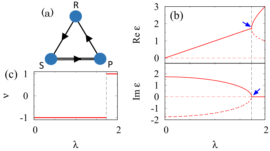
Figure 1: (a): Sketch of the RPS cycle. The arrows denote dominance relationship between the strategies for $\lambda=0$; “R” beats “S”; “S” beats “P”; “P” beats “R”. The second terms proportional to $\lambda$ are introduced between sites connected by the double line. (b): The real- and imaginary-parts of eigenvalues as functions of $\lambda$. An eigenvalue of $A(\lambda)$ is zero for an arbitrary $\lambda$ (see horizontal dashed lines). (c): The $\mathbb{Z}_{2}$-invariant characterizing the EP. The dashed vertical lines in panels (b) and (c) denote $\lambda=\lambda_{\mathrm{c}}$.

Dynamical properties and the EP. Suppose that a large number of players repeat the above game whose dynamics is described by the replicator equation [see Eq. (10)]. In this case, the EP governs the dynamical behaviors when the population density slightly deviates from a fixed point; the population density shows an oscillatory behavior for $0\leq\lambda<\lambda_{\mathrm{c}}$, while such a behavior disappear for $\lambda_{\mathrm{c}}<\lambda$ due to the emergence of the EP.

Firstly, we linearize the replicator equation. When a large number of players repeat the game, the time-evolution is described by the replicator equation

$$\partial_{t}\bm{e}^{T}_{I}\cdot\bm{x} = \bm{e}^{T}_{I}\cdot\bm{x}\left(\bm{e}^{T}_{I}A\bm{x}-\bm{x}^{T}A\bm{x}\right),$$ (10)

where $\bm{x}$ denotes the population density ($\sum_{I}x_{I}=1$), and $\bm{e}_{I}$ is a unit vector whose $I$-th element is unity. The second term vanishes when the payoff matrix $A$ is anti-symmetric. However, in order to access the non-Hermitian topology, the second term is inevitable which makes the argument in Ref. Yoshida et al., 2021 unavailable.

Nevertheless, we can still obtain the following linearized equation

$$\partial_{t}\delta\bm{x} = \frac{1}{N_{0}}A\delta\bm{x},$$ (11)

which is mathematically equivalent to the Schrödinger equation. This mathematical equivalence reveals that the dynamics of the RPS cycle (i.e., a classical system) can be understood in terms of quantum physics. Here, $\delta\bm{x}$ is defined as $\delta\bm{x}=\bm{x}-\bm{c}$ with $\bm{c}=(1,1,\ldots,1)^{T}/N_{0}$, and $N_{0}$ denotes dimensions of the matrix $A$. Key ingredients are the following relations:

$$\sum_{J}A_{IJ}=0\quad \mathrm{and} \quad\sum_{J}A_{JI}=0,$$ (12)

for an arbitrary $I$. This equation guarantees that $\bm{c}$ denotes a fixed point. Linearizing the replicator equation around this fixed point, we obtain Eq. (11) as detailed in the “Methods”.

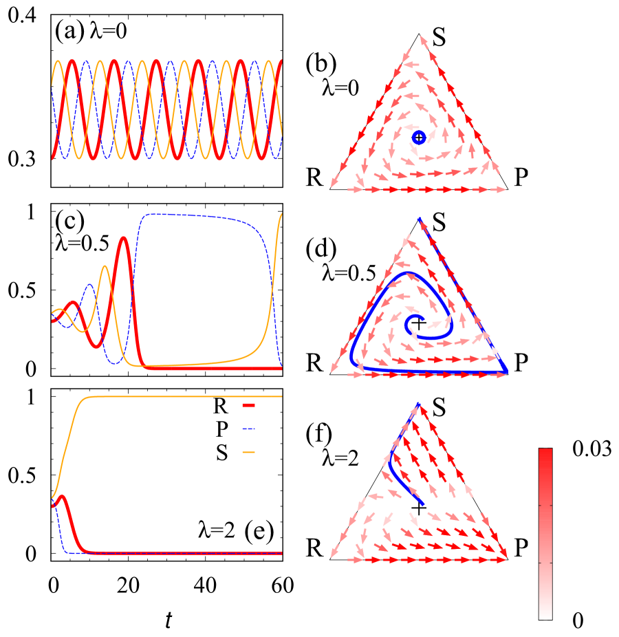
Figure 2: Dynamical properties of the RPS game (7). Panels (a), (c), and (e) display the time-evolution of the population $\bm{x}$ for $\lambda=0$, $0.5$, and $2$, respectively. The data are obtained by employing a fourth order Runge-Kutta method Süli & Mayers (2003) with discretized time $t_{n}=n\Delta t_{\mathrm{RK}}$ with $\Delta t_{\mathrm{RK}}=0.05$. We set the initial condition as $\bm{x}(t=0)=(1-\delta_{0},1+\delta_{0}/2,1+\delta_{0}/2)/3$ with $\delta_{0}=0.1$. The time-evolution is computed up to $t_{n}=120$. Panels (b), (d), and (f) are phase plots for $\bm{x}$. The arrows denote the direction of the dynamics $(\Delta x_{1},\Delta x_{2},\Delta x_{3})$ which is computed by $\Delta x_{I}=x_{I}(\bm{e}^{T}_{I}A\bm{x}-\bm{x}^{T}A\bm{x})\Delta t$ with $\Delta t=0.1$. The black crosses denote the fixed point specified by $\bm{c}=(1,1,1)/3$. In panels (b), (d), and (f), the blue line denotes the population density $\bm{x}(t)$ plotted in panels (a), (c), and (e), respectively.

The linearized replicator equation indicates that the dynamics is governed by the spectrum of $A$. In particular, the imaginary-part of the eigenvalues results in oscillatory behaviors.

To verify the above statement, we numerically solve the replicator equation (10). Figure 2 plots the time-evolution of the population density for several values of $\lambda$. For $\lambda=0$, the matrix $A(\lambda)$ is reduced to the payoff matrix of the standard zero-sum RPS game. In this case, the eigenvalues of $A$ are pure imaginary, which results in the oscillatory behavior [see Fig. 2(a)]. This oscillatory behavior is also observed in the phase plot [see Fig. 2(b)], where the orbit forms a closed loop. The above oscillatory behavior is also observed for $\lambda=0.5$ [see Figs. 2(c) and 2(d)], which is due to the imaginary-part of the eigenvalues. We also note that the deviation $\delta\bm{x}$ is enhanced as $t$ increases, which is because the real-part of the eigenvalues is positive [see Fig. 1(b)]. Further increasing $\lambda$ induces the EP [see Fig. 1(b)], and the eigenvalues become real. Correspondingly, the above oscillatory behavior is not observed for $\lambda=2$ [see Figs. 2(e) and 2(f)], The above numerical data verify that the EP governs the dynamics around the fixed point $\bm{c}$; the oscillatory behavior of the RPS cycle disappears as the EP emerges. We note that for $\lambda<0$, the fixed point corresponds to evolutionary stable strategy. A similar EP emerges also in this case which governs the dynamics.

We close this part with three remarks. Firstly, so far, we have seen the emergence of the EP in the RPS game by changing $\lambda$. We note that symmetry-protected exceptional rings are also observed by introducing an additional parameter (see Sec. S2 of Supplemental Material [68]), whose topology is also characterized by the $\mathbb{Z}_{2}$-invariant $\nu$. Secondly, although Refs. Szabó & Fáth, 2007; Szolnoki et al., 2014; Dobramysl et al., 2018; Szolnoki et al., 2020 discusses topology of interaction networks among strategies (i.e., interaction topology), it differs from the topology discussed in this paper. Thirdly, we note that EPs are also reported for active matters Sone et al. (2020); Tang et al. (2021). We would like to stress, however, that significance of this paper is to reveal the emergence of the EPs and how they affect the dynamics in systems of the evolutionary game theory which describes the population density of biological systems and human societies.

Skin effect in an RPS chain. Now, we discuss a one-dimensional system showing the skin effect whose origin is the non-trivial topology characterized by the winding number Zhang et al. (2020); Okuma et al. (2020). Because of this non-trivial topology, switching from the periodic boundary condition (PBC) to the open boundary condition (OBC) significantly changes the spectrum. Correspondingly, almost of all right eigenstates are localized around the right edge which are called skin modes.

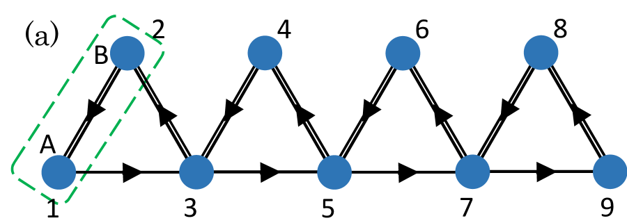
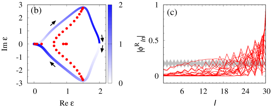
Figure 3: (a): Sketch of the RPS chain for $L_{x}=4$ with an additional site at $I=9$. The arrows describes payoffs. The terms proportional to $\lambda$ are introduced between sites connected by double lines. As shown in this panel, $I$ takes $I=1,2,3,\ldots$. For the PBC, $I+2L_{x}=I$ holds. Dashed line denotes the unit cell. For $J=1,2,\ldots$, $R_{2I-1}=R_{2I}$ holds. (b): Spectrum of the RPS chain for $\lambda=-0.5$. The data colored with blue are obtained under the PBC. Here, the shade of color denotes $k/\pi$. The data denoted by red dots are obtained for $L_{x}=15$ and the OBC. (c): Amplitude of the right eigenvectors $\phi^{\mathrm{R}}_{In}$ ($n=1,2,\ldots,2L_{x}$) as functions of $I$ for $L_{x}=15$. Red (gray) lines denote data for the OBC (PBC).

The above skin effect can be observed in an RPS chain illustrated in Fig. 3(a). Applying the Fourier transformation, the payoff matrix is written as

$$A(k) = \left(\begin{array}[]{cc}0&1-e^{-ik}\\ -1+e^{ik}&-2i\sin k\end{array}\right)+\lambda\left(\begin{array}[]{cc}-2&1+e^{-ik}\\ 1+e^{ik}&-2\end{array}\right),$$ (17)

under the PBC. Here, $\bm{x}_{k}$ is defined as $\bm{x}^{T}_{k}=(x_{k\mathrm{A}},x_{k\mathrm{B}})$ with $x_{k\alpha}=\frac{1}{L_{x}}\sum_{R_{I}}e^{ikR_{I}}x_{R_{I}\alpha}$ and $\alpha=\mathrm{A},\mathrm{B}$. Sets of $R_{I}$ and $\alpha_{I}$ are specified by $I$ ($x_{I}=x_{R_{I}\alpha_{I}}$). For the explicit form of the payoff matrix in the real-space, see Sec. S3 of Supplemental Material [68].

Figure 3(b) plots the spectrum of the payoff matrix for $\lambda=-0.5$. When the PBC is imposed, eigenvalues form a loop structure as denoted by blue lines in Fig. 3(b). Accordingly, the winding number Gong et al. (2018); Zhang et al. (2020); Okuma et al. (2020) defined as

$$W = \oint\frac{dk}{2\pi i}\partial_{k}\log\mathrm{det}[A(k)-\epsilon_{\mathrm{ref}}\mbox{1}\mbox{l}],$$ (19)

takes $-1$ for $\epsilon_{\mathrm{ref}}=1$, which implies the skin effect. Indeed, imposing the OBC significantly changes the spectrum [see red dots in Fig. 3(b)]. Correspondingly, almost all of the right eigenvectors are localized around the edges, meaning the emergence of skin modes [see Fig. 3(c)].

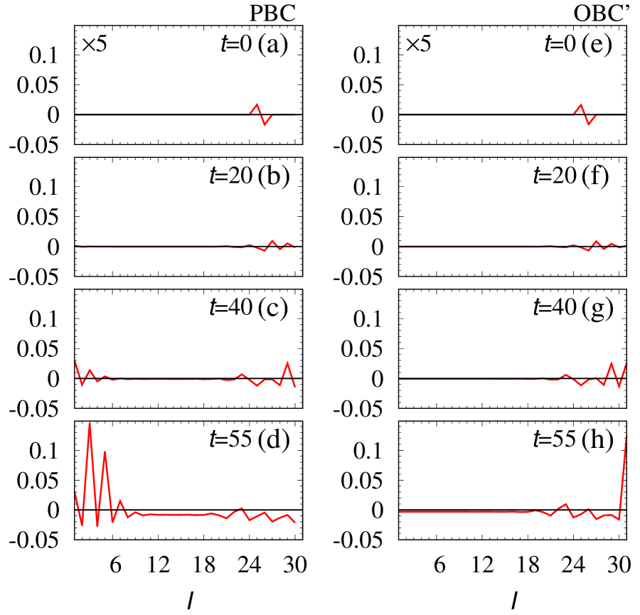
Figure 4: Time-evolution of the population density $\delta\bm{x}(t)=\bm{x}(t)-\bm{c}$ for $\lambda=-0.5$ and $L_{x}=15$. The horizontal axis denotes $I$. (a)-(d) [(e)-(f)]: The time-evolution under the PBC [OBC’]. The data in panels (a) and (e) are multiplied by 5. The data are obtained by employing the fourth order Runge-Kutta method Süli & Mayers (2003) with discretized time $t_{n}=n\Delta t_{\mathrm{RK}}$ with $\Delta t_{\mathrm{RK}}=0.05$. We set the initial condition so that $N_{0}x_{I}(0)$ takes $1+\delta_{0}$ and $1-\delta_{0}$ with $\delta_{0}=0.1$ for $I=25$ and $I=26$, respectively. For the other $I$, $N_{0}x_{I}(0)$ takes 1. Here, $N_{0}$ is chosen so that $\sum_{I}x_{I}(0)=1$ holds.

The above data [Figs. 3(b) and 3(c)] indicate that the skin effect is observed in the RPS chain. Here, we note that the spectrum and skin modes are almost unchanged under the following perturbation to the edges (see Sec. S3 of Supplemental Material [68]): attaching site at $I=2L_{x}+1$ and tuning diagonal elements to $A_{II}=\lambda$ only for $I=1,2L_{x}+1$ so that Eq. (12) holds [see Fig. 3(a)]. We refer to this boundary condition as OBC’.

The above skin effect results in striking dynamical properties: the directive propagation of the population density in the bulk and the enhancement of the population density only around the right edge. The directive propagation is observed by imposing the PBC. Figures 4(a)-4(d) indicate that the propagation only to the right direction is enhanced. This phenomenon can be understood by noting the following facts as well as linearized approximation: (i) as $t$ increases, each mode is enhanced corresponding to $\mathrm{Re}\epsilon_{n}$; (ii) the group velocity of each mode is proportional to $-\partial_{k}\mathrm{Im}\epsilon_{n}$. Because of the loop structure resulting in $W=-1$, the modes propagating to the right are more enhanced than the ones propagating to the left.

The enhancement of the population density at the right edge is observed by imposing OBC’. We note that Eq. (12) is satisfied for OBC’ while it is not for OBC. As shown in Figs. 4(e)-4(h), the population density around the right edge is enhanced as $t$ increases. This phenomenon is due to the skin modes whose eigenvalues satisfy $\mathrm{Re}\epsilon_{n}>0$. The above dynamical behaviors are unique to non-Hermitian systems; turning off $\lambda$, $iA(\lambda=0)$ becomes Hermitian and the above behaviors disappear (see Sec. S3 of Supplemental Material [68]).

We close this part with two remarks. Firstly, we note that a similar behaviors can be observed for another RPS chain, implying ubiquity of the skin effect (see Sec. S4 of Supplemental Material [68]). Secondly, Ref. Knebel et al., 2020 has analyzed an RPS chain whose payoff matrix is Hermitian up to the imaginary unit $i$. We would like to stress, however, that our aim is to observe non-Hermitian topological phenomena which are not accessible with the model in Ref. Knebel et al., 2020. In this non-Hermitian case, we need to take into account the second term of Eq. (10).

Discussion We have proposed a new platform of non-Hermitian topology in an interdisciplinary field, i.e., RPS cycles described by the evolutionary game theory. Specifically, by analyzing the payoff matrix, we have demonstrated the emergence of the EP and the skin effect which are representative non-Hermitian topological phenomena. In addition, our linearized replicator equation has revealed that the EP governs the dynamics of the population density around the fixed point. Furthermore, we have discovered the striking dynamical phenomenon in the RPS chain: the directive propagation of the population density in the bulk and the enhancement of the population density only around the right edge which are induced by the skin effect.

Our results pose several future directions which we discuss below. The experimental observation is one of the central issues. In particular, our results provide a first step toward the observation of the non-Hermitian topology beyond natural science because the game theory describes a wide variety of systems from biological systems Kirkup & Riley (2004); Sinervo & Lively (1996) to human societies Rosas (2010); Szolnoki et al. (2012); Szolnoki & Perc (2013); Wang et al. (2013); Perc et al. (2017); for instance, dynamics of human cooperation has been discussed in Refs. Szolnoki et al., 2012; Szolnoki & Perc, 2013. The experimental observation in such a system is considered to be a significant step to the application of topological phenomena beyond natural science. In addition, as is the case of equatorial wave Delplace et al. (2017), our result may provide a novel perspective of well-known phenomena for biological systems such as bacteria Kirkup & Riley (2004) and side-blotched lizards Sinervo & Lively (1996); dynamics of such systems may be understood in terms of exceptional points. We also note that the topological classification for systems described by the game theory is also a crucial issue to be addressed.

Methods
Derivation of the linearized replicator equation. Here, we derive Eq. (11). We start with noting Eq. (12) results in the relations $A\bm{c}=0$ and $\bm{c}^{T}A=0$ which mean that $\bm{c}=(1,1,1,\ldots,1)^{T}/N_{0}$ is a fixed point. By making use of the above relations we have

$$\partial_{t}\bm{e}^{T}_{I}\cdot\delta\bm{x}$$

$$=\bm{e}^{T}_{I}\cdot(\bm{c}+\delta\bm{x})\left[\bm{e}^{T}_{I}A(\bm{c}+\delta\bm{x})-(\bm{c}+\delta\bm{x})^{T}A(\bm{c}+\delta\bm{x})\right]$$

$$=\bm{e}^{T}_{I}\cdot(\bm{c}+\delta\bm{x})\left(\bm{e}^{T}_{I}A\delta\bm{x}-\delta\bm{x}^{T}A\delta\bm{x}\right)$$

$$\sim(\bm{e}^{T}_{I}\cdot\bm{c})\bm{e}^{T}_{I}A\delta\bm{x}.$$ (20)

From the second to the third line, we have used the relations $A\bm{c}=0$ and $\bm{c}A=0$. In the last line, we have discarded the second and third order terms of $\delta\bm{x}$.

Because $(\bm{e}^{T}_{I}\cdot\bm{c})=1/N_{0}$ for an arbitrary $I$, we have

$$\partial_{t}\delta\bm{e}^{T}_{I}\cdot\bm{x} \sim \frac{1}{N_{0}}\bm{e}^{T}_{I}A\delta\bm{x},$$ (21)

which is equivalent to Eq. (11).

Acknowledgements. This work is supported by JSPS Grant-in-Aid for Scientific Research on Innovative Areas “Discrete Geometric Analysis for Materials Design”: Grant No. JP20H04627. This work is also supported by JSPS KAKENHI Grants No. JP17H06138, No. JP20K14371, and No. JP21K13850.

Author contributions T.Y., T. M., and Y. H. planned the project. T. Y. performed the calculations. T.Y., and T. M., and Y. H. were involved in the discussion of the materials and the preparation of the manuscript.

Competing financial interests The authors declare no competing interests.

S1 $PT$ symmetry

Here, we briefly review topological properties under $PT$ symmetry (i.e., symmetry described by the product of the time-reversal operation and inversion). When the system is $PT$ symmetric, the Bloch Hamiltonian $h(\bm{k})$ satisfies

$$PTh(\bm{k})PT^{-1} = h(\bm{k}),$$ (S1)

with an anti-unitary operator $PT=U_{PT}\mathcal{K}$, a unitary matrix $U_{PT}$, and $\bm{k}$ denoting the momentum. Here, each of the time-reversal operation and the spatial inversion flips the momentum ($\bm{k}\to-\bm{k}$), and thus, their product does not flip $\bm{k}$.

Equation (S1) results in the following constraint on the eigenvalue $\epsilon_{n}$ ($n=1,2,\ldots$)

$$\epsilon_{n}=\epsilon^{*}_{n^{\prime}}\ \mathrm{or} \ \epsilon_{n}\in\mathbb{R}.$$ (S2)

The above equation is obtained by a straightforward calculation. Suppose that $|\psi_{n}(\bm{k})\rangle_{R}$ and $\epsilon_{n}(\bm{k})$ are a right eigenvector and an eigenvalue of $h(\bm{k})$, $h(\bm{k})|\psi_{n}(\bm{k})\rangle_{R}=\epsilon_{n}(\bm{k})|\psi_{n}(\bm{k})\rangle_{R}$. Then, $PT|\psi_{n}(\bm{k})\rangle_{R}$ is an eigenstate with eigenvalue $\epsilon^{*}_{n}$ because

$$h(\bm{k})PT|\psi_{n}(\bm{k})\rangle_{R} = PTh(\bm{k})|\psi_{n}(\bm{k})\rangle_{R}$$ (S3)

$$= \epsilon^{*}_{n}(\bm{k})PT|\psi_{n}(\bm{k})\rangle_{R},$$

holds. Therefore, we obtain Eq. (S2).

Now, let us discuss the topology for $PT^{2}=1$. When a point-gap opens at $\epsilon_{\mathrm{ref}}\in\mathbb{R}$ [i.e., $\mathrm{det}(h-\epsilon_{\mathrm{ref}})\neq 0$ holds], the system may possess topological properties which are characterized by the following zero-dimensional $\mathbb{Z}_{2}$-invariant $\nu^{\prime}$

$$\nu^{\prime} = -\mathrm{sgn}[\mathrm{det}(h-\epsilon_{\mathrm{ref}})],$$ (S4)

with $\mathrm{sgn}(x)$ takes $1$ ($-1$) for $x>0$ ($x<0$). For $\epsilon_{\mathrm{ref}}=\epsilon_{\mathrm{EP}}$ ($\epsilon_{\mathrm{EP}}=\sqrt{3}$), $\nu^{\prime}$ and $\nu$ defined in Eq. (3) characterizes the same topology of Eq. (1); because $\nu^{\prime}=\prod_{n}(\epsilon_{n}-\epsilon_{\mathrm{\mathrm{ref}}})$ holds, we have $\nu^{\prime}$ taking $1$ ($-1$) for $\lambda>\lambda_{\mathrm{c}}$ ($\lambda<\lambda_{\mathrm{c}}$).

S2 Symmetry-protected exceptional rings in an RPS cycle

We demonstrate the emergence of a symmetry-protected exceptional rings in evolutionary game theory. Consider an extended RPS cycle whose payoff matrix is written as

$$A(\lambda,\kappa) = A(\lambda)+\kappa\left(\begin{array}[]{ccc}1&0&-1\\ 0&0&0\\ -1&0&1\end{array}\right),$$ (S8)

with $\lambda,\kappa\in\mathbb{R}$.

We can block-diagonalize the matrix $A$. Applying the unitary transformation with

$$V = \left(\begin{array}[]{ccc}\frac{1}{\sqrt{3}}&\frac{1}{\sqrt{2}}&\frac{1}{\sqrt{6}}\\ \frac{1}{\sqrt{3}}&-\frac{1}{\sqrt{2}}&\frac{1}{\sqrt{6}}\\ \frac{1}{\sqrt{3}}&0&\frac{-\sqrt{2}}{\sqrt{3}}\end{array}\right),$$ (S12)

we have

$$V^{T}A(\lambda,\kappa)V = \left(\begin{array}[]{ccc}0&0&0\\ 0&0&-\sqrt{3}\\ 0&\sqrt{3}&0\end{array}\right)+\lambda\left(\begin{array}[]{ccc}0&0&0\\ 0&\frac{1}{2}&-\frac{\sqrt{3}}{2}\\ 0&-\frac{\sqrt{3}}{2}&\frac{3}{2}\end{array}\right)+\kappa\left(\begin{array}[]{ccc}0&0&0\\ 0&\frac{1}{2}&\frac{\sqrt{3}}{2}\\ 0&\frac{\sqrt{3}}{2}&\frac{3}{2}\end{array}\right).$$ (S22)

Diagonalizing the above matrix, we have eigenvalues $0$ and

$$\epsilon_{\pm} = (\lambda+\kappa)\pm\sqrt{\frac{3}{4}(\lambda-\kappa)^{2}+\frac{1}{4}(\lambda+\kappa)^{2}-3}.$$ (S23)

We note that for $\kappa=0$, the EP emerges at $\lambda=\lambda_{\mathrm{c}}=\sqrt{3}$.

Figure S1(a) [S1(b)] plots the real- [imaginary] part of $\epsilon_{\pm}$. These figures indicate the emergence of the symmetry-protected exceptional rings; EPs, where the two bands touch both for the real- and the imaginary-parts, form a ring. We also note that $\nu$ takes $-1$ ($1$) inside (outside) of the ring, elucidating the topological protection.

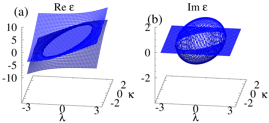
Figure S1: (a) and (b): The real- and imaginary-parts of $\epsilon_{\pm}$. The data colored with blue (dark blue) represents $\epsilon_{+}$ ($\epsilon_{-}$).

The above results verify the emergence of the symmetry-protected exceptional rings in the extended RPS cycle.

S3 Details of the RPS chain

We discuss details of the RPS chain defined in the main text. Under the OBC’, the payoff matrix is written as

$$A(\lambda) = A_{0}+\lambda B.$$ (S24)

We have introduced an additional site at $I=9$ [see Fig. 3(a)] for $L_{x}=4$. Hence, the vector $\bm{x}$ consists of nine components, $\bm{x}=(x_{1},x_{2},x_{3},\cdots,x_{9})^{T}$. Here, $A_{0}$ and $B$ are defined as

$$A_{0} = \left(\begin{array}[]{ccccc}A_{0\mathrm{d}}&A^{T}_{0\mathrm{c}}&0&0&0\\ A_{0\mathrm{c}}&A_{0\mathrm{d}}&A^{T}_{0\mathrm{c}}&0&0\\ 0&A_{0\mathrm{c}}&A_{0\mathrm{d}}&A^{T}_{0\mathrm{c}}&0\\ 0&0&A_{0\mathrm{c}}&A_{0\mathrm{d}}&A^{T}_{0\mathrm{cR}}\\ 0&0&0&A_{0\mathrm{cR}}&0\end{array}\right),$$ (S25f)

with

$$A_{0\mathrm{d}}=\left(\begin{array}[]{cc}0&1\\ -1&0\end{array}\right),\quad A_{0\mathrm{c}}=\left(\begin{array}[]{cc}-1&0\\ 1&0\end{array}\right),\quad A_{0\mathrm{cR}}=\left(\begin{array}[]{cc}1&-1\end{array}\right),$$ (S25l)

and

$$B = \left(\begin{array}[]{ccccc}B_{\mathrm{dL}}&B^{T}_{\mathrm{c}}&0&0&0\\ B_{\mathrm{c}}&B_{\mathrm{d}}&B^{T}_{\mathrm{c}}&0&0\\ 0&B_{\mathrm{c}}&B_{\mathrm{d}}&B^{T}_{\mathrm{c}}&0\\ 0&0&B_{\mathrm{c}}&B^{T}_{\mathrm{d}}&B^{T}_{\mathrm{cR}}\\ 0&0&0&B^{T}_{\mathrm{cR}}&-1\end{array}\right),$$ (S26f)

with

$$B_{\mathrm{d}}=\left(\begin{array}[]{cc}-2&1\\ 1&-2\end{array}\right),\quad B_{\mathrm{c}}=\left(\begin{array}[]{cc}0&1\\ 0&0\end{array}\right),\quad B_{\mathrm{dL}}=\left(\begin{array}[]{cc}-1&1\\ 1&-2\end{array}\right),\quad B_{\mathrm{cR}}=\left(\begin{array}[]{cc}0&1\end{array}\right),$$ (S26n)

respectively. In addition, we have imposed $B_{11}=B_{99}=-1$ to satisfy Eq. (6).

In Fig. S2, we can see that the spectrum and amplitude of the right eigenvectors for OBC’ are similar to those for OBC, which indicates the robustness of the skin effect against perturbations. This is because the non-Hermitian topology induces the skin effect. We also note that $\bm{c}=(1,1,\ldots,1)/31$ is the right eigenvector for $L_{x}=15$ [see Fig. S2(b)] because Eq. (6) holds under OBC’.

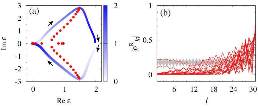
Figure S2: Spectrum and amplitude of right eigenvectors under the OBC’. (a): The spectrum for $\lambda=-0.5$ and $L_{x}=15$. (b):Amplitude of the right eigenvectors $\phi^{\mathrm{R}}_{In}$ ($n=1,2,\ldots,2L_{x}+1$) as functions of $I$ for $L_{x}=15$. The data are plotted in a similar way to Fig. 3.

When Eq. (6) is satisfied, the replicator equation (4) can be linearized as discussed in the main text. In this case, the dynamics is governed by

$$i\partial_{t}\delta\bm{x}(t) = H\delta\bm{x}(t),$$ (S27)

with $H=iA/N_{0}$ [see also Eq. (5)] which is mathematically equivalent to the Schrödinger equation. In quantum systems, the group velocity and the lifetime are written as $\partial_{k}\mathrm{Re}E_{n}(k)$ and $1/\mathrm{Im}E_{n}(k)$ ($\mathrm{Im}E_{n}(k)>0$), respectively. Here, $E_{n}(k)$ $(n=1,2,\ldots)$ denotes eigenvalues of $H$.

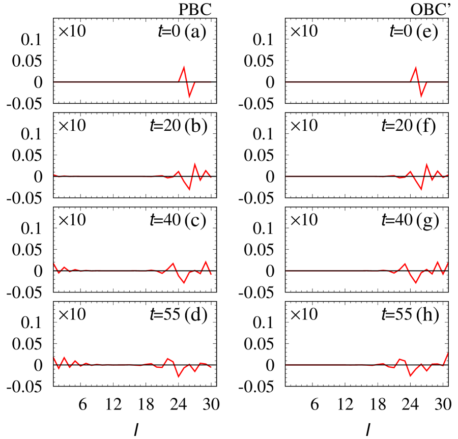
Figure S3: Time-evolution of the population density $\delta\bm{x}(t)=\bm{x}(t)-\bm{c}$ for $\lambda=0$ and $L_{x}=15$. The horizontal axis denotes $I$. (a)-(d) [(e)-(f)]: The time-evolution under the PBC [OBC’]. The data in all panels are multiplied by 10. These data are obtained in the same way as those of Fig. 4.

Figure S3 displays the dynamical properties for $\lambda=0$ where the payoff matrix is anti-Hermitian. Because all eigenvalues $\epsilon$’s are pure imaginary, the directive perpetration which arises from the real-part of the eigenvalues $\epsilon$’s is not observed. In addition, no localized mode is enhanced due to the absence of skin modes.

S4 Another RPS chain

We introduce another RPS chain [see Fig. S4(a)] exhibiting the skin effect. For $L_{x}=5$, the payoff matrix is written as

$$A = \left(\begin{array}[]{ccccc}A_{0}&0&0&0&A^{\prime}_{\mathrm{c}}\\ A_{\mathrm{c}}&A_{0}&0&0&0\\ 0&A_{\mathrm{c}}&A_{0}&0&0\\ 0&0&A_{\mathrm{c}}&A_{0}&0\\ 0&0&0&A_{\mathrm{c}}&A_{0}\end{array}\right),$$ (S28f)

with

$$A_{0} = \left(\begin{array}[]{ccc}d&0&r_{2}\\ r_{3}&d&0\\ 0&r_{1}&d\end{array}\right),$$ (S28j)

$$A_{\mathrm{c}} = \left(\begin{array}[]{ccc}0&0&r_{4}\\ 0&0&0\\ 0&0&0\end{array}\right),$$ (S28n)

and the vector $$\bm{x}$$ consists of fifteen components,

$$\bm{x} = (x_{1},x_{2},x_{3},\cdots,x_{15})^{T}.$$ (S28o)

Here, $A^{\prime}_{\mathrm{c}}$ is equal to $A_{\mathrm{c}}$ (the zero matrix) under the PBC (OBC).

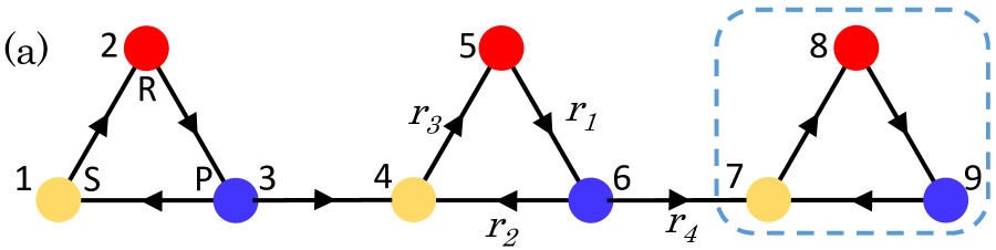
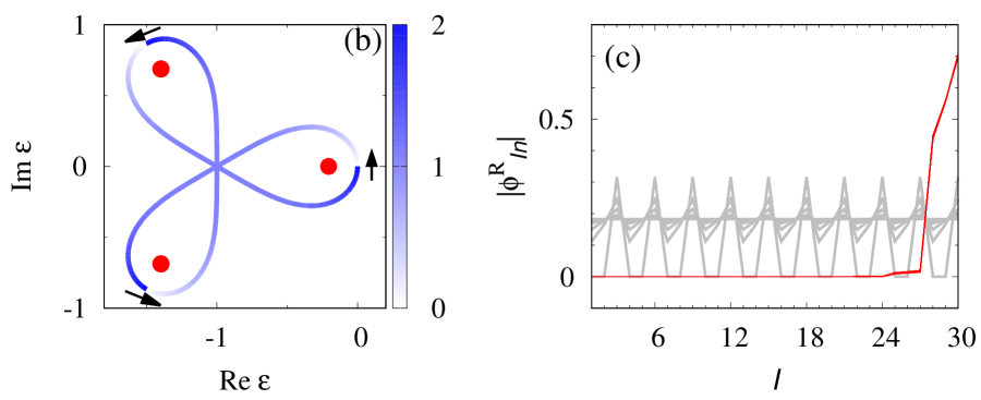
Figure S4: (a): Sketch of the RPS chain for $L_{x}=3$. The arrows and $r$’s describe payoffs. Here, $A_{II}=d$ for an arbitrary $I$. As shown in this panel, $I$ takes $I=1,2,\ldots,3L_{x}$. For the PBC, $I+3L_{x}=I$ holds. Dashed line denotes the unit cell. For $J=1,2,\ldots,L_{x}$, $R_{3J-2}=R_{3J-1}=R_{3J}=J$ holds. (b): Spectrum of the RPS chain for $(r_{1},r_{2},r_{3},r_{4},d)=(1,1/2,1,1/2,-1)$. The data colored with blue are obtained under the PBC. Here, the shade of color denotes $k/\pi$. The data colored with red are obtained for $L_{x}=10$ and the OBC. (c): Amplitude of the right eigenvectors $|\phi^{\mathrm{R}}_{In}|$ $n=1,2,\ldots,3L_{x}$ as functions of $I$ for $L_{x}=10$. Red (gray) lines denote data for the OBC (PBC). For the OBC, all of the eigenvectors are localized around the right edge.

Applying the Fourier transformation, the payoff matrix is written as

$$A(k) = \left(\begin{array}[]{ccc}d&0&r_{2}+r_{4}e^{ik}\\ r_{3}&d&0\\ 0&r_{1}&d\end{array}\right),$$ (S32)

under the PBC. Here, $\bm{x}_{k}$ is defined as $\bm{x}^{T}_{k}=(x_{k\mathrm{S}},x_{k\mathrm{R}},x_{k\mathrm{P}})$ with $x_{ks}=\frac{1}{L_{x}}\sum_{R_{I}}e^{ikR_{I}}x_{R_{I}s}$ and $s=\mathrm{R},\mathrm{P},\mathrm{S}$. Sets of $R_{I}$ and $s_{I}$ are specified by $I$ ($x_{I}=x_{R_{I}s_{I}}$).

Figure S4(b) plots the spectrum of the payoff matrix for $(r_{1},r_{2},r_{3},r_{4},d)=(1,1/2,1,1/2,-1)$. When the PBC is imposed, eigenvalues form a loop structure as denoted by blue lines in Fig. S4(b). Accordingly, the winding number [Eq. (8)] takes $1$ for $\epsilon_{\mathrm{ref}}=0.5$, which implies the skin effect. Indeed, imposing the OBC significantly changes the spectrum [see red dots in Fig. S4(b)]. Correspondingly, all of the right eigenvectors are localized around the edges, meaning the emergence of skin modes [see Fig. S4(c)]. The above data [Figs. S4(b) and S4(c)] indicate that the skin effect is observed in this RPS chain as well. The essentially same results of eigenvalues and eigenvectors are also obtained for $(r_{1},r_{2},r_{3},r_{4},d)=(2,2,2,2,1)$. For this parameter set, the chain is composed of an ordinary RPS cycles Wang et al. (2014) whose payoff matrix is written as $\left(\begin{array}[]{ccc}1&0&2\\ 2&1&0\\ 0&2&1\end{array}\right)$.

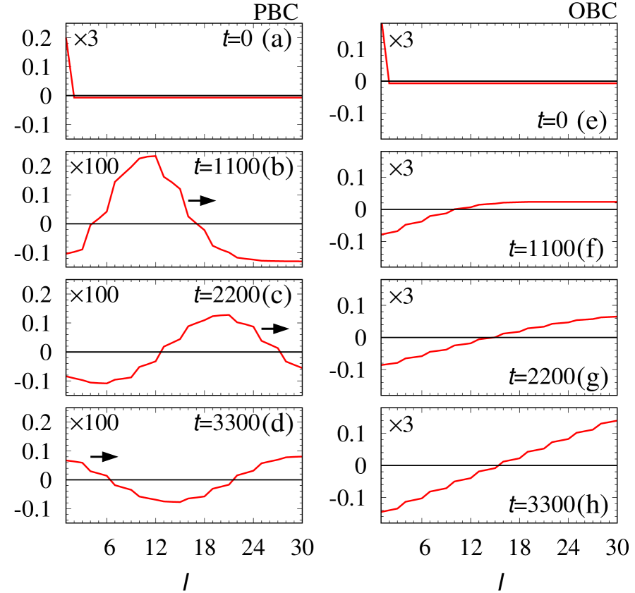
Figure S5: The time-evolution of the population density $\delta\bm{x}(t)=\bm{x}(t)-\bm{c}$ for $(r_{1},r_{2},r_{3},r_{4},d)=(1,1/2,1,1/2,-1)$ and $L_{x}=10$. The horizontal axis denotes $I$. (a)-(d) [(e)-(f)]: The time-evolution under the PBC [OBC]. The data in panels (b)-(d) [(a) and (e)-(h)] are multiplied by $100$ [$3$]. The data are obtained by employing the fourth order Runge-Kutta method Süli & Mayers (2003) with discretized time $t_{n}=n\Delta t_{\mathrm{RK}}$ with $\Delta t_{\mathrm{RK}}=0.05$. We set the initial condition as $\delta\bm{x}(0)=\frac{\delta_{0}}{(3L_{x}-1)3L_{x}}(3L_{x}-1,-1,-1,\ldots,-1)$ with $\delta_{0}=2$.

As discussed in main text, the non-Hermitian topology characterized by $W=1$ induces the directive propagation under the PBC [see Fig. S5(a)-S5(d)] where Eq. (6) is satisfied for this parameter set. We also note that under the OBC, the players prefer to be localized around the right edge for large $t$ [see Fig. S5(e)-S5(f)]. However, introducing the edges violates Eq. (6) which prevents us from mapping Eq. (4) to the Schrödinger equation; introducing perturbations around the edge does not help to recover Eq. (6) for this model.

References

- Kane & Mele (2005) C. L. Kane & E. J. Mele topological order and the quantum spin hall effect. Phys. Rev. Lett., 95, 146802 (2005).
- Bernevig et al. (2006) B. A. Bernevig, T. L. Hughes & S.-C. Zhang Quantum spin hall effect and topological phase transition in hgte quantum wells. Science, 314, 1757–1761 (2006).
- König et al. (2007) M. König, S. Wiedmann, C. Brüne, A. Roth, H. Buhmann, L. W. Molenkamp, X.-L. Qi & S.-C. Zhang Quantum spin hall insulator state in hgte quantum wells. Science, 318, 766–770 (2007).
- Hasan & Kane (2010) M. Z. Hasan & C. L. Kane Colloquium. Rev. Mod. Phys., 82, 3045–3067 (2010).
- Qi & Zhang (2011) X.-L. Qi & S.-C. Zhang Topological insulators and superconductors. Rev. Mod. Phys., 83, 1057–1110 (2011).
- Klitzing et al. (1980) K. v. Klitzing, G. Dorda & M. Pepper New method for high-accuracy determination of the fine-structure constant based on quantized hall resistance. Phys. Rev. Lett., 45, 494–497 (1980).
- Thouless et al. (1982) D. J. Thouless, M. Kohmoto, M. P. Nightingale & M. d. Nijs Quantized hall conductance in a two-dimensional periodic potential. Phys. Rev. Lett., 49, 405–408 (1982).
- Halperin (1982) B. I. Halperin Quantized hall conductance, current-carrying edge states, and the existence of extended states in a two-dimensional disordered potential. Phys. Rev. B, 25, 2185–2190 (1982).
- Hatsugai (1993) Y. Hatsugai Chern number and edge states in the integer quantum hall effect. Phys. Rev. Lett., 71, 3697–3700 (1993).
- Haldane & Raghu (2008) F. D. M. Haldane & S. Raghu Possible realization of directional optical waveguides in photonic crystals with broken time-reversal symmetry. Phys. Rev. Lett., 100, 013904 (2008).
- Wang et al. (2009) Z. Wang, Y. Chong, J. D. Joannopoulos & M. Soljacic Observation of unidirectional backscattering-immune topological electromagnetic states. Nature, 461, 772 EP – (2009).
- Fu et al. (2010) J.-X. Fu, R.-J. Liu & Z.-Y. Li Robust one-way modes in gyromagnetic photonic crystal waveguides with different interfaces. Applied Physics Letters, 97, 041112 (2010).
- Ozawa et al. (2019) T. Ozawa, H. M. Price, A. Amo, N. Goldman, M. Hafezi, L. Lu, M. C. Rechtsman, D. Schuster, J. Simon, O. Zilberberg & I. Carusotto Topological photonics. Rev. Mod. Phys., 91, 015006 (2019).
- Prodan & Prodan (2009) E. Prodan & C. Prodan Topological phonon modes and their role in dynamic instability of microtubules. Phys. Rev. Lett., 103, 248101 (2009).
- Kane & Lubensky (2013) C. L. Kane & T. C. Lubensky Topological boundary modes in isostatic lattices. Nature Physics, 10, 39 EP – (2013).
- Kariyado & Hatsugai (2015) T. Kariyado & Y. Hatsugai Manipulation of dirac cones in mechanical graphene. Scientific Reports, 5, 18107 (2015).
- Süsstrunk & Huber (2015) R. Süsstrunk & S. D. Huber Observation of phononic helical edge states in a mechanical topological insulator. Science, 349, 47–50 (2015).
- Delplace et al. (2017) P. Delplace, J. B. Marston & A. Venaille Topological origin of equatorial waves. Science, 358, 1075–1077 (2017).
- Sone & Ashida (2019) K. Sone & Y. Ashida Anomalous topological active matter. Phys. Rev. Lett., 123, 205502 (2019).
- Yoshida & Hatsugai (2021) T. Yoshida & Y. Hatsugai Bulk-edge correspondence of classical diffusion phenomena. Scientific Reports, 11, 888 (2021).
- Knebel et al. (2020) J. Knebel, P. M. Geiger & E. Frey Topological phase transition in coupled rock-paper-scissors cycles. Phys. Rev. Lett., 125, 258301 (2020).
- Yoshida et al. (2021) T. Yoshida, T. Mizoguchi & Y. Hatsugai Chiral edge modes in evolutionary game theory: A kagome network of rock-paper-scissors cycles. Phys. Rev. E, 104, 025003 (2021).
- Weibull (1997) J. W. Weibull Evolutionary game theory. MIT press (1997).
- Sigmund (2011) K. Sigmund Evolutionary game dynamics, vol. 69. American Mathematical Society (2011).
- Kirkup & Riley (2004) B. C. Kirkup & M. A. Riley Antibiotic-mediated antagonism leads to a bacterial game of rock-pape-scissors in vivo. Nature, 428, 412–414 (2004).
- Rosas (2010) A. Rosas Evolutionary game theory meets social science: Is there a unifying rule for human cooperation? Journal of Theoretical Biology, 264, 450–456 (2010).
- Wang et al. (2013) Z. Wang, S. Kokubo, J. Tanimoto, E. Fukuda & K. Shigaki Insight into the so-called spatial reciprocity. Phys. Rev. E, 88, 042145 (2013).
- Perc et al. (2017) M. Perc, J. J. Jordan, D. G. Rand, Z. Wang, S. Boccaletti & A. Szolnoki. Physics Reports, 687, 1–51 (2017).
- Hatano & Nelson (1996) N. Hatano & D. R. Nelson Localization transitions in non-hermitian quantum mechanics. Phys. Rev. Lett., 77, 570–573 (1996).
- Bender & Boettcher (1998) C. M. Bender & S. Boettcher Real spectra in non-hermitian hamiltonians having symmetry. Phys. Rev. Lett., 80, 5243–5246 (1998).
- Gong et al. (2018) Z. Gong, Y. Ashida, K. Kawabata, K. Takasan, S. Higashikawa & M. Ueda Topological phases of non-hermitian systems. Phys. Rev. X, 8, 031079 (2018).
- Kawabata et al. (2019) K. Kawabata, K. Shiozaki, M. Ueda & M. Sato Symmetry and topology in non-hermitian physics. Phys. Rev. X, 9, 041015 (2019).
- Bergholtz et al. (2021) E. J. Bergholtz, J. C. Budich & F. K. Kunst Exceptional topology of non-hermitian systems. Rev. Mod. Phys., 93, 015005 (2021).
- Ashida et al. (2020) Y. Ashida, Z. Gong & M. Ueda Non-hermitian physics. Advances in Physics, 69, 249–435 (2020).
- Rotter (2009) I. Rotter A non-hermitian hamilton operator and the physics of open quantum systems. Journal of Physics A: Mathematical and Theoretical, 42, 153001 (2009).
- Shen et al. (2018) H. Shen, B. Zhen & L. Fu Topological band theory for non-hermitian hamiltonians. Phys. Rev. Lett., 120, 146402 (2018).
- Kozii & Fu (2017) V. Kozii & L. Fu Non-hermitian topological theory of finite-lifetime quasiparticles: Prediction of bulk fermi arc due to exceptional point. arXiv preprint arXiv:1708.05841 (2017).
- Yoshida et al. (2018) T. Yoshida, R. Peters & N. Kawakami Non-hermitian perspective of the band structure in heavy-fermion systems. Phys. Rev. B, 98, 035141 (2018).
- Budich et al. (2019) J. C. Budich, J. Carlström, F. K. Kunst & E. J. Bergholtz Symmetry-protected nodal phases in non-hermitian systems. Phys. Rev. B, 99, 041406 (2019).
- Okugawa & Yokoyama (2019) R. Okugawa & T. Yokoyama Topological exceptional surfaces in non-hermitian systems with parity-time and parity-particle-hole symmetries. Phys. Rev. B, 99, 041202 (2019).
- Yoshida et al. (2019) T. Yoshida, R. Peters, N. Kawakami & Y. Hatsugai Symmetry-protected exceptional rings in two-dimensional correlated systems with chiral symmetry. Phys. Rev. B, 99, 121101 (2019).
- Zhou et al. (2019) H. Zhou, J. Y. Lee, S. Liu & B. Zhen Exceptional surfaces in pt-symmetric non-hermitian photonic systems. Optica, 6, 190–193 (2019).
- Kimura et al. (2019) K. Kimura, T. Yoshida & N. Kawakami Chiral-symmetry protected exceptional torus in correlated nodal-line semimetals. Phys. Rev. B, 100, 115124 (2019).
- Yoshida & Hatsugai (2019) T. Yoshida & Y. Hatsugai Exceptional rings protected by emergent symmetry for mechanical systems. Phys. Rev. B, 100, 054109 (2019).
- Delplace et al. (2021) P. Delplace, T. Yoshida & Y. Hatsugai Symmetry-protected higher-order exceptional points and their topological characterization. arXiv preprint arXiv:2103.08232 (2021).
- Yao & Wang (2018) S. Yao & Z. Wang Edge states and topological invariants of non-hermitian systems. Phys. Rev. Lett., 121, 086803 (2018).
- Lee & Thomale (2019) C. H. Lee & R. Thomale Anatomy of skin modes and topology in non-hermitian systems. Phys. Rev. B, 99, 201103 (2019).
- Zhang et al. (2020) K. Zhang, Z. Yang & C. Fang Correspondence between winding numbers and skin modes in non-hermitian systems. Phys. Rev. Lett., 125, 126402 (2020).
- Okuma et al. (2020) N. Okuma, K. Kawabata, K. Shiozaki & M. Sato Topological origin of non-hermitian skin effects. Phys. Rev. Lett., 124, 086801 (2020).
- Lee et al. (2019) J. Y. Lee, J. Ahn, H. Zhou & A. Vishwanath Topological correspondence between hermitian and non-hermitian systems: Anomalous dynamics. Phys. Rev. Lett., 123, 206404 (2019).
- Borgnia et al. (2020) D. S. Borgnia, A. J. Kruchkov & R.-J. Slager Non-hermitian boundary modes and topology. Phys. Rev. Lett., 124, 056802 (2020).
- Yoshida et al. (2020) T. Yoshida, T. Mizoguchi & Y. Hatsugai Mirror skin effect and its electric circuit simulation. Phys. Rev. Research, 2, 022062 (2020).
- Guo et al. (2009) A. Guo, G. J. Salamo, D. Duchesne, R. Morandotti, M. Volatier-Ravat, V. Aimez, G. A. Siviloglou & D. N. Christodoulides Observation of -symmetry breaking in complex optical potentials. Phys. Rev. Lett., 103, 093902 (2009).
- Zhen et al. (2015) B. Zhen, C. W. Hsu, Y. Igarashi, L. Lu, I. Kaminer, A. Pick, S.-L. Chua, J. D. Joannopoulos & M. Soljacic Spawning rings of exceptional points out of dirac cones. Nature, 525, 354 EP – (2015).
- Hassan et al. (2017) A. U. Hassan, B. Zhen, M. Soljačić, M. Khajavikhan & D. N. Christodoulides Dynamically encircling exceptional points: Exact evolution and polarization state conversion. Phys. Rev. Lett., 118, 093002 (2017).
- Zhou et al. (2018) H. Zhou, C. Peng, Y. Yoon, C. W. Hsu, K. A. Nelson, L. Fu, J. D. Joannopoulos, M. Soljačić & B. Zhen Observation of bulk fermi arc and polarization half charge from paired exceptional points. Science, 359, 1009–1012 (2018).
- Zyuzin & Zyuzin (2018) A. A. Zyuzin & A. Y. Zyuzin Flat band in disorder-driven non-hermitian weyl semimetals. Phys. Rev. B, 97, 041203 (2018).
- Papaj et al. (2019) M. Papaj, H. Isobe & L. Fu Nodal arc of disordered dirac fermions and non-hermitian band theory. Phys. Rev. B, 99, 201107 (2019).
- Shen & Fu (2018) H. Shen & L. Fu Quantum oscillation from in-gap states and a non-hermitian landau level problem. Phys. Rev. Lett., 121, 026403 (2018).
- Matsushita et al. (2019) T. Matsushita, Y. Nagai & S. Fujimoto Disorder-induced exceptional and hybrid point rings in weyl/dirac semimetals. Phys. Rev. B, 100, 245205 (2019).
- Hofmann et al. (2020) T. Hofmann, T. Helbig, F. Schindler, N. Salgo, M. Brzezińska, M. Greiter, T. Kiessling, D. Wolf, A. Vollhardt, A. Kabaši et al. Reciprocal skin effect and its realization in a topolectrical circuit. Phys. Rev. Research, 2, 023265 (2020).
- Helbig et al. (2020) T. Helbig, T. Hofmann, S. Imhof, M. Abdelghany, T. Kiessling, L. W. Molenkamp, C. H. Lee, A. Szameit, M. Greiter & R. Thomale Generalized bulk-boundary correspondence in non-hermitian topolectrical circuits. Nature Physics, 16, 747–750 (2020).
- Matsushita et al. (2021) T. Matsushita, Y. Nagai & S. Fujimoto Spectrum collapse of disordered dirac landau levels as topological non-hermitian physics. Journal of the Physical Society of Japan, 90, 074703 (2021).
- Tainaka (1993) K. Tainaka Paradoxical effect in a three-candidate voter model. Physics Letters A, 176, 303–306 (1993).
- Juul et al. (2012) J. Juul, K. Sneppen & J. Mathiesen Clonal selection prevents tragedy of the commons when neighbors compete in a rock-paper-scissors game. Phys. Rev. E, 85, 061924 (2012).
- Szolnoki et al. (2014) A. Szolnoki, J. Vukov & M. c. v. Perc From pairwise to group interactions in games of cyclic dominance. Phys. Rev. E, 89, 062125 (2014).
- Szolnoki & Perc (2016) A. Szolnoki & M. Perc Biodiversity in models of cyclic dominance is preserved by heterogeneity in site-specific invasion rates. Scientific Reports, 6, 38608 (2016).
- Süli & Mayers (2003) E. Süli & D. F. Mayers An introduction to numerical analysis. Cambridge university press (2003).
- Szabó & Fáth (2007) G. Szabó & G. Fáth Evolutionary games on graphs. Physics Reports, 446, 97–216 (2007).
- Szolnoki et al. (2014) A. Szolnoki, M. Mobilia, L.-L. Jiang, B. Szczesny, A. M. Rucklidge & M. Perc Cyclic dominance in evolutionary games: a review. Journal of the Royal Society Interface, 11, 20140735 (2014).
- Dobramysl et al. (2018) U. Dobramysl, M. Mobilia, M. Pleimling & U. C. Täuber Stochastic population dynamics in spatially extended predator–prey systems. J. Phys. A: Math. Theor., 51, 063001 (2018).
- Szolnoki et al. (2020) A. Szolnoki, B. F. d. Oliveira & D. Bazeia Pattern formations driven by cyclic interactions: A brief review of recent developments. Europhys. Lett., 131, 68001 (2020).
- Sone et al. (2020) K. Sone, Y. Ashida & T. Sagawa Exceptional non-hermitian topological edge mode and its application to active matter. Nature Communications, 11, 5745 (2020).
- Tang et al. (2021) E. Tang, J. Agudo-Canalejo & R. Golestanian Topology protects chiral edge currents in stochastic systems. Phys. Rev. X, 11, 031015 (2021).
- Sinervo & Lively (1996) B. Sinervo & C. M. Lively The rock–paper–scissors game and the evolution of alternative male strategies. Nature, 380, 240–243 (1996).
- Szolnoki et al. (2012) A. Szolnoki, M. c. v. Perc & G. Szabó Defense mechanisms of empathetic players in the spatial ultimatum game. Phys. Rev. Lett., 109, 078701 (2012).
- Szolnoki & Perc (2013) A. Szolnoki & M. c. v. Perc Correlation of positive and negative reciprocity fails to confer an evolutionary advantage: Phase transitions to elementary strategies. Phys. Rev. X, 3, 041021 (2013).

References

- Wang et al. (2014) Z. Wang, B. Xu & H.-J. Zhou Social cycling and conditional responses in the rock-paper-scissors game. Scientific Reports, 4, 5830 (2014).
- Süli & Mayers (2003) E. Süli & D. F. Mayers An introduction to numerical analysis. Cambridge university press (2003).