X-ray Flares Raising upon Magnetar Plateau as an Implication of a Surrounding Disk of Newborn Magnetized Neutron Star

Abstract

The X-ray flares have usually been ascribed to long-lasting activities of the central engine of gamma-ray bursts (GRBs), e.g., fallback accretion. The GRB X-ray plateaus, however, favor a millisecond magnetar central engine. The fallback accretion can be significantly suppressed due to the propeller effect of a magnetar. Therefore, if the propeller regime cannot resist the mass flow onto the surface of the magnetar efficiently, the X-ray flares raise upon the magnetar plateau would be hinted. In this work, such peculiar cases are connected to the accretion process of a magnetar, and an implication for magnetar-disc structure is given. We investigate the repeating accretion process with multi-flare GRB 050730, and give a discussion for the accreting induced variation of the magnetic field in GRB 111209A. Two or more flares exhibit in the GRB 050730, GRB 060607A, and GRB 140304A; by adopting magnetar mass $M=1.4~{}M_{\odot}$ and radius $R=12~{}\rm km$, the average mass flow rates of the corresponding surrounding disk are $3.53\times 10^{-4}~{}M_{\odot}~{}\rm s^{-1}$, $4.23\times 10^{-4}~{}M_{\odot}~{}\rm s^{-1}$, and $4.33\times 10^{-4}~{}M_{\odot}~{}\rm s^{-1}$, and the corresponding average sizes of the magnetosphere are $5.01~{}\rm\times 10^{6}cm$, $6.45~{}\rm\times 10^{6}cm$, and $1.09~{}\rm\times 10^{7}cm$, respectively. A statistic analysis that contains 8 GRBs within 12 flares shows that the total mass loading in single flare is $\sim 2\times 10^{-5}~{}M_{\odot}$. In the lost mass of a disk, there are about 0.1% used to feed a collimated jet.

1 Introduction

Based on the duration distribution, Gamma-ray bursts (GRBs) are divided into long-duration ($T_{90}>2~{}\rm s$) and short-duration ($T_{90}<2~{}\rm s$) types (Kouveliotou et al. 1993). Long GRBs (lGRBs) are believed to originate from the core collapse of a massive star (Woosley 1993; Galama et al. 1998; MacFadyen & Woosley 1999; Bloom et al. 1999; Zhang et al. 2003) and to associate with the explosion of core-collapse supernovae (Stanek et al. 2003; Hjorth et al. 2003; Campana et al. 2006). That the merger of two compact objects creates the short GRBs (sGRBs; e.g., Paczynski 1986; Eichler et al. 1989; Narayan et al. 1992; Gehrels et al. 2005; Hjorth et al. 2005) was also confirmed by the association of gravitational wave (GW) event, i.e., GW170817 and GRB 170817A (Abbott et al. 2017b, a). A rapidly rotating and strongly magnetized neutron star (NS) is thought to be born as a central engine, the so called magnetar, whatever lGRBs or sGRBs (Usov 1992; Thompson 1994; Dai & Lu 1998; Wheeler et al. 2000; Zhang & Mészáros 2001; Lyons et al. 2010; Metzger et al. 2008, 2011; Bucciantini et al. 2012). The studies of soft gamma-ray repeater (SGR) showed that the surface dipole magnetic field of a magnetar can be as high as $10^{15}~{}\rm G$ (e.g., Kouveliotou et al. 1998, 1999; Woods et al. 1999). A corotating magnetosphere of the magnetized NS preventing the plasma accretion and throwing away the accreting materials were figured as propeller (Illarionov & Sunyaev 1975; Campana et al. 1998). A competing process of accretion and propeller was figured in the recent studies (e.g., Ekşi et al. 2005; Gompertz et al. 2014; Lin et al. 2021). However, the coexistence of accretion and outflow was also suggested by some of the magnetohydrodynamic (MHD) simulative studies (e.g., Goodson et al. 1997; Romanova et al. 2005, 2009, 2018; Ustyugova et al. 2006). In these studies, a two-component outflow, propeller-driven conical wind and accretion-feed collimated jet, is seen for a rapidly rotating star scenario. Bernardini et al. (2013) attributed the precursor and the prompt emission of GRBs to a jet that forms in the accretion phase.

A canonical GRB X-ray afterglow can be composed of five components (Nousek et al. 2006; Zhang et al. 2006), in which rapid decay, normal decay and jet break track the properties of a jet, however, the shallow decay (or plateau) and the X-ray flares were proposed to connect a long-lasting central engine. Large sample investigations showed that there are one or more X-ray flares seen in about one third of GRB afterglows (Falcone et al. 2007; Chincarini et al. 2007, 2010), the time domain analyses for its lightcurve imply that the X-ray flares have an “internal” origin, and a new idea for restart the central engine is required (Burrows et al. 2005a; Fan & Wei 2005; Liang et al. 2006; Lazzati & Perna 2007). An intermittent hyperaccreting disk surrounding a black hole (BH) seems to be a great candidate (King et al. 2005; Perna et al. 2006). Cao et al. (2014) imported a competition between the magnetic field and the neutrino dominated accretion flow (NDAF) to avoid a fragmentary hyperaccreting disk. By comparing with the diffusion timescale of magnetic field, a time interval between the two successive accreting episodes is about 0.2 s, and the mass accretion rate can be as high as $\sim 1~{}M_{\odot}\rm~{}s^{-1}$ for a external magnetic field $B=10^{14}~{}\rm G$. Interestingly, the initially accumulated shells onto blast wave to produce the observed shallow decay was also investigated. However, the observed X-ray afterglows are too dark as compared to the prediction of the model (Maxham & Zhang 2009). A statistic analysis of Swift/XRT data showed that the lightcurve decay slope $-0.75$ distinguishes between the normal decay segment and the shallow decay segment (Liang et al. 2008). A continuous energy injection into the forward shock explains the shallow decay successfully (Evans et al. 2009). However, the X-ray plateau followed by sharp decay in some cases invoke an explanation with the internal energy dissipation of a magnetar wind (e.g., Coroniti 1990; Usov 1992, 1994; Troja et al. 2007; Rowlinson et al. 2010, 2013, 2014; Lü & Zhang 2014; Lü et al. 2015). The end of the magnetar plateau is featured as a steeper decay for the spindown process of a magnetar or a very steep decay for the collapse of magnetar into a BH, where the typical slopes are $\sim-2$ (Zhang & Mészáros 2001) and $<-3$ (Liang et al. 2007; Lyons et al. 2010; Rowlinson et al. 2010), respectively. Then, a re-brightening catching the end of the very steep decay symbolizing the fallback material onto the newborn BH was proposed (Chen et al. 2017).

The connection between X-ray flares and the millisecond magnetar has suggested by Dai et al. (2006), but more credible evidence is expected to be excavated. Some peculiar cases display a coexistence of X-ray flares and magnetar plateau, which persuade us to connect between the magnetar accreting from the surrounding disc and the spindown process of a magnetar. If the magnetic dipole (MD) radiation of a magnetar is in progress, the charged particles would form a magnetosphere surrounding the magnetar due to the affection of strong magnetic field. The propeller regime keeps away the fallback material to form a dense disk next to the magnetosphere. However, an unstable channelled flow would be led by gravitational force along the magnetic field line onto the polar cap of the central magnetar. In the meantime, owing to the magnetic and centrifugal forces, a small fraction of the accreting material penetrates into the opened polar magnetic field line and feeds a relativistic collimated jet, then a considerable X-ray flare is induced. In this work, we argue that the X-ray flares raising upon the magnetar plateau can be used to connect the accretion process of a magnetar and to lead an implication for magnetar-disc structure. The properties of the jet, magnetar, and disk are investigated with both the special cases and a small sample study. In Section 2, we review the activities of newborn magnetized NS, both case study and sample analysis are presented in Section 3, conclusions and discussions are organized in Section 4. A $\Lambda$CDM cosmology with parameters $H_{0}=70~{}\rm{km\ s^{-1}\ Mpc^{-1}}$, $\Omega_{M}=0.30$, and $\Omega_{\Lambda}=0.70$ is adopted.

2 Millisecond Magnetar Activities

By adopting a rotating progenitor model (Heger et al. 2000), the particle hydrodynamics simulation showed that the initial period $P_{0}$ of a newly born NS is $\sim 100$ ms, and drops to $\sim 2$ ms after a short cooling (Fryer & Heger 2000). A considerable rotational energy is stored in newly born millisecond NS,

$$E_{rot}=\frac{1}{2}I\Omega^{2}\simeq 2\times 10^{52}M_{1.4}R_{6}^{2}P_{-3}^{-2}~{}\rm erg,$$ (1)

where $I$ is the moment of inertia, for a NS holds mass $M$ and radius $R$, it can be written as $I=0.35MR^{2}$ (Lattimer & Prakash 2001). The spin period $P=2\pi/\Omega$, where $\Omega$ is the angular frequency of the NS, and the notation $Q_{n}=Q/10^{n}$ in cgs units, furthermore $M_{1.4}=M/1.4M_{\odot}$. For a magnetar central engine scenario, its rotational energy lose as a magnetar wind or an ejecta and is observed in the X-ray afterglows,

$$-\dot{E}_{rot}=I\Omega\dot{\Omega}=L=f_{b}L_{\rm iso,X}/\eta,$$ (2)

where $L_{\rm iso,X}$ is isotropic X-ray luminosity. The efficiency of rotational energy to the observed X-ray emission $\eta$ holds significantly different value for different process. For the Swift/XRT (Burrows et al. 2005b), about $1\%$ jet energy can emit into the observation window in a GRB prompt emission analogous to the GRB radiative efficiency (e.g., Zhang et al. 2007; Wang et al. 2015), and as high as $50\%$ rotational energy can be observed for a magnetar wind (Metzger et al. 2011; Lü & Zhang 2014). $f_{b}=1-$cos$\theta$ is the beaming factor, where $\theta$ is opening angle. The opening angle of a magnetar wind $\theta_{\rm dip}$ is also worth to budget. It should larger than a jet of GRBs $\sim 0.1~{}\rm rad$ ($\sim 6^{\circ}$; Frail et al. 2001), but smaller than a low speed conical wind $\sim 30^{\circ}-40^{\circ}$ (Romanova et al. 2009). A study for the internal dissipation of magnetar wind showed that the observed X-ray emission typical less than $10\%$ when a saturation Lorentz $\Gamma_{sat}\geq 100$ is adopted (Xiao & Dai 2019). According to the study of GRB magnetar central engines by Rowlinson et al. (2014), when adopting the observed plateau holds $\sim 5\%$ ($\eta_{\rm dip}=0.05$) rotational energy, the beaming angle is $\sim 10^{\circ}$ ($f_{b}=0.015$). Furthermore, the observed X-ray energy fraction $\eta_{\rm fla}=0.05$, and a moderate beaming angle $\theta_{\rm fla}=10^{\circ}$ for the X-flares are adopted in this work.

2.1 Magnetic Dipole Radiation

For a magnetar holds surface magnetic field strength $B$ and initial spin period $P_{0}$, its spindown luminosity $L$ is featured as a plateau ($t\ll\tau$) followed by a sharp decay ($t\gg\tau$) (Zhang & Mészáros 2001),

$$L=L_{0}(1+\frac{t}{\tau})^{-2},$$ (3)

where the characteristic spindown luminosity $L_{0}$ and the timescale $\tau$ is given by

$$L_{0} = 1.0\times 10^{49}B_{15}^{2}P_{0,-3}^{-4}R_{6}^{6}~{}\rm erg~{}s^{-1},$$

$$\tau = 2.05\times 10^{3}I_{45}B_{15}^{-2}P_{0,-3}^{2}R_{6}^{-6}~{}\rm s.$$ (4)

When considering the affection of multiple energy dissipating mechanisms and the spectral evolution of radiative process, the slope of a sharp decay may hold a very different value (Lasky et al. 2017; Lü et al. 2018, 2019; Xiao & Dai 2019).

2.2 Accretion Process of a Magnetar

The surface magnetic field strength of millisecond magnetar is as high as $\sim 10^{15}$ G. It would affect the ionized materials that close to the surface of magnetar and boost the forming of a corotating magnetosphere. The material inside the magnetosphere is dominated by the magnetic pressure, and the magnetic pressure in any given radius $r$ is written as $P_{m}=\mu^{2}/8\pi r^{6}$, where the MD moment of the magnetar is written as $\mu=BR^{3}$. An accretion flow from the disk exerts a ram pressure $P_{\rm ram}=\dot{M}_{\rm disk}(2GM)^{1/2}/{8\pi r^{5/2}}$, where $\dot{M}_{\rm disk}$ is the mass flow rate of the disk, and $G$ is the gravitational constant. Therefore, the position where the material pressure comparable with the magnetic pressure is defined as Alvén radius (Davidson & Ostriker 1973; Ekşi et al. 2005),

$$R_{A} = \left(\frac{\mu^{4}}{2GM\dot{M}_{\rm disk}^{2}}\right)^{1/7}$$ (5)

$$= 2.5\times 10^{6}M_{1.4}^{-1/7}R_{6}^{12/7}B_{14}^{4/7}\dot{M}_{\rm disk,-5}^{-2/7}~{}\rm cm.$$

At the corotating radius $R_{c}$, the material keeps the same angular frequency with magnetar without magnetic force considered,

$$R_{c} = \left(\frac{GM}{\Omega^{2}}\right)^{1/3}$$ (6)

$$= 1.7\times 10^{6}M_{1.4}^{1/3}P_{-3}^{2/3}~{}\rm cm.$$

Hence, when the magnetic pressure can not keep the disk as far as corotating position, e.g., $R_{A}<R_{c}$, an unstable channelled flow would be led by gravitational force along the magnetic line onto the polar region of the central magnetar. There are two parts of the energy transmitted from accretion materials to a magnetar, the kinetic energy and the gravitational potential energy. Considering a continuous constant accretion rate, the energy transmission can be written as

$$\dot{E}_{acc} = E_{\rm start}-E_{\rm end}$$ (7)

$$= \frac{1}{2}\dot{M}_{\rm acc}\left(R_{A}^{2}\Omega_{\rm K,A}^{2}-R^{\prime 2}\Omega^{2}\right)$$

$$-GM\dot{M}_{\rm acc}\left(\frac{1}{R_{A}}-\frac{1}{R}\right),$$

where $\dot{M}_{\rm acc}$ is mass flow rate of the accretion onto the magnetar, $\Omega_{\rm K,A}=(GM/R_{A}^{3})^{1/2}$ is the Keplerian frequency at the Alfvén radius, and one has $\Omega_{\rm K,A}>\Omega$ for $R_{A}<R_{c}$. When the accretion materials inhabit the polar cap of the magnetar, the radius of its moment of inertia is marked as $R^{\prime}$, and here has $R^{\prime}\leq R<R_{A}$. For a typical NS with surface magnetic field $B=10^{15}~{}\rm G$ and a mass flow rate of the disk $\dot{M}_{\rm disk}<10^{-3}~{}M_{\odot}$, one has $R_{A}>2.5R$. Therefore, the approximate result is given as

$$\dot{E}_{\rm acc} \approx \frac{1}{2}GM\dot{M}_{\rm acc}\frac{1}{R_{A}}+GM\dot{M}_{\rm acc}\left(\frac{1}{R}-\frac{1}{R_{A}}\right)$$ (8)

$$\approx GM\dot{M}_{\rm acc}\frac{1}{R}.$$

Hence, we find that the most of energy is donated by gravitational potential energy. Accreting materials transmit its kinetic and gravitational potential energy onto the magnetar, then the latter spins up.

A magnetized, rapidly rotating star accompanied by an accretion disk was studied by the MHD simulative investigations (e.g., Goodson et al. 1997; Romanova et al. 2005, 2009, 2018; Ustyugova et al. 2006). These studies suggested that the mass flow to the star and to the outflow can take place at the same time, and a two-component outflow, propeller-driven conical wind and accretion-feed collimated jet, can be seen in the polar region. In the accretion phase, most of funnelled accreting flow on to the pole of star. However, owing to the magnetic and centrifugal force, a part of it flows into the opened magnetic lines and feeds a collimated jet (Goodson & Winglee 1999; Romanova et al. 2009). The mass flow rates rely on the magnetar parameters, and the relations are approximated as (Ustyugova et al. 2006)

$$\dot{M}_{\rm wind} \propto\Omega^{2.6}\mu^{0.9},$$ (9)

$$\dot{M}_{\rm jet} \propto\Omega\mu^{0.2},$$

$$\dot{M}_{\rm acc} \propto\Omega^{-5}\mu^{-1.3},$$

$$\dot{M}_{\rm disk} \propto\Omega^{-2.2}\mu^{0.9},$$

where, the mass flow rates of the collimated jet and the conical wind are marked as $\dot{M}_{\rm jet}$ and $\dot{M}_{\rm wind}$, respectively. Comparing with the propeller-driven conical wind, the low-density, high-velocity, magnetic dominated, collimated jet is more energetic. For a protostar, if considering the jet is a component that poloidal velocities $\nu_{p}>1.5\nu_{K}$, where $\nu_{K}$ is Keplerian velocity, the jet component carries about $1\%$ of the total outflowing mass and $13\%$ of the total lost angular momentum of the star (Romanova et al. 2009). Therefore, it is easy to get that about $69\%$ lost rotational energy is carried by the jet component. A same outflow scenario is adopted in this work.

In the propeller regime, a propeller efficiency is organized as (Romanova et al. 2018)

$$f_{\rm eff}=\frac{\dot{\bar{M}}_{\rm out}}{\dot{\bar{M}}_{\rm acc}+\dot{\bar{M}}_{\rm out}}$$ (10)

where $\dot{\bar{M}}_{\rm out}$ and $\dot{\bar{M}}_{\rm acc}$ are time-averaged mass flow rate of the outflow and accretion onto the star. $\dot{\bar{M}}_{\rm out}$ relates to a considered minimum outflowing poloidal velocities $\nu_{\rm min}$, when $\nu_{\rm min}>\nu_{\rm esc}$ is considered, the average propeller efficiency has $f_{\rm eff}=0.0006\omega^{4.01}_{s}$, where $\nu_{\rm esc}$ is escape velocity and $\nu_{\rm esc}\sim 1.5\nu_{K}$, $\omega_{s}=\Omega/\Omega_{K,A}$ is a fitness parameter (Romanova et al. 2018). In this scenario, the outflow can ascribe to the collimated jet, that is $\dot{M}_{\rm out}=\dot{M}_{\rm jet}$, where $\dot{M}_{\rm out}$ is mass flow rate of the outflow. By adopting $\omega_{s}=1.2$, the accretion mass flow rate and the mass lost rate of disk can be estimated with the mass flow rate of a jet,

$$\dot{M}_{\rm acc}=832\dot{M}_{\rm jet},$$

$$\dot{M}_{\rm dis}=931\dot{M}_{\rm jet}.$$ (11)

The one should note that the disk oscillations were also suggested by the mentioned MHD simulative studies, therefore the $\omega_{s}$ may get a prominent change at the before and after the accretion process.

Since some studies have suggested that the central magnetar could spin up by the accretion toque and spin down by the propeller torque (e.g., Ekşi et al. 2005; Gompertz et al. 2014; Lin et al. 2021), it is necessary to budget the energy income and output of a magnetar. The total mass loading in the jet $M_{\rm jet}=\int{\dot{M}_{\rm jet}}dt$ can be estimated with $E_{\rm fla}=M_{\rm jet}c^{2}\gamma$, where $c$ is the speed of the light, $E_{\rm fla}$ is the total energy for a single event, and $\gamma$ is the bulk Lorentz factor of the jet. By adopting the bulk Lorentz factor of the jet component $\gamma=100$ (Maxham & Zhang 2009), the lost and gathered energy of the magnetar can be budgeted, $\zeta=(E_{\rm jet}/0.69)/E_{\rm acc}\sim 3$. Since too many uncertainty in the estimation, and a not significant advantage is charged by the lost energy, the spin evolution of the central magnetar is not considered in this work. To estimate mass loading in the jet, the $E_{\rm fla}$ can be derived with the observed isotropic luminosity of X-ray flares $L_{\rm fla,X,iso}$, that is

$$E_{\rm fla}=f_{b}\int{L_{\rm fla,X,iso}}dt/\eta_{\rm fla}.$$ (12)

3 Sample study and the tests of physical parameters

The X-ray afterglow data are derived from the UK Swift Science Data centra (UKSSDC; Evans et al. 2009). The selected cases present a X-ray plateau followed by a sharp decay, which is identified as the internal energy dissipation of a magnetar wind. Ahead of the sharp decay, the prominent X-ray flares, the internal shock (Maxham & Zhang 2009) which originates from the accreting fed collimated jet, raise upon the magnetar plateau. The lightcurves are fitted with a smooth broken power law function

$$F=F_{0}\left[\left(\frac{t}{t_{b}}\right)^{-\omega\alpha_{1}}+\left(\frac{t}{t_{b}}\right)^{-\omega\alpha_{2}}\right]^{-1/\omega},$$ (13)

where the sharpness parameter marked as $\omega$, the constant flux at break time $t_{b}$ is written as $F_{b}=F_{0}\cdot 2^{-1/\omega}$, and the decay indices before and after $t_{b}$ is described as $\alpha_{1}$ and $\alpha_{2}$.

3.1 GRB 050730

The weak lGRB 050730 triggered Swift/BAT at 19:58:23 on 2005-07-30 (Holland et al. 2005) ($T_{0}$ in the following), with prompt emission duration $T_{90}(15-150~{}\rm keV)=157\pm 18~{}s$ at redshift $z=3.967$ (Chen et al. 2005; Rol et al. 2005; Holman et al. 2005; Prochaska et al. 2005; D’Elia et al. 2005). The average photon index for its mean photon arrival time $T_{0}+17681$ $\rm s$ is $\Gamma=1.58$. Its X-ray afterglow featured as three X-ray flares competing with the long-duration plateau and followed by a sharp decay ($\alpha_{2}=2.77$). We derive the isotropic luminosity by using $L(t)=4\pi D_{L}^{2}f(t)k(z)$ where $D_{L}$ is the luminosity distance, $f(t)$ is the observed X-ray flux and $k(z)=(1+z)^{\Gamma-2}$ is the cosmological $k$-correction factor (Bloom et al. 2001; Şaşmaz Muş et al. 2019). The lightcurve is presented in Figure 1. For the MD radiation model, the characteristic spindown luminosity and time scale are $L_{0}=(2.81\pm 0.49)\times 10^{49}\times f_{b}/\eta~{}\rm erg~{}\rm s^{-1}$ and $\tau=(7.65\pm 0.49)\times 10^{3}/(1+z)~{}\rm s$, respectively. The surface magnetic field and the initial spin period can be estimated with Eq. (4), and ones have $B=(1.16\pm 0.13)\times 10^{15}~{}\rm G$ and $P_{0}=(1.48\pm 0.14)~{}\rm ms$. The observed X-ray fluence of the flares integrate since $T_{0}+193~{}\rm s$, $T_{0}+327~{}\rm s$, and $T_{0}+598~{}\rm s$ for flare $\rm I$, flare $\rm II$ and flare $\rm III$, and ones have $7.24\times 10^{-8}~{}\rm erg~{}\rm cm^{-2}$, $2.08\times 10^{-7}~{}\rm erg~{}\rm cm^{-2}$, and $1.23\times 10^{-7}~{}\rm erg~{}\rm cm^{-2}$, respectively.

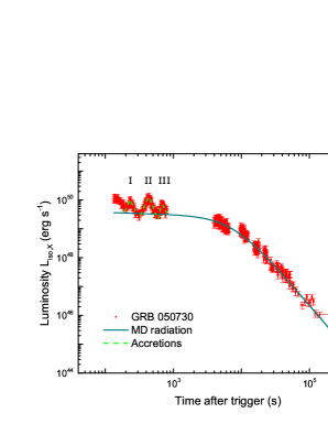
Figure 1: Lightcurve of GRB 050730, the multi-flare phenomenon is carried to connect the repeating accretion process of a magnetar.

The jet forming process is still ambiguous. In Section 2, we assume that the accretion onto the magnetar feeds a collimated jet to create the considerable X-ray flares. In this scenario, the accreting material supplies its kinetic energy and gravitational potential energy to keep the period of the central magnetar without a significant change, the total energy of the observed X-ray flare equal to those gravitational potential energy quantitatively. By adopting a magnetar with mass $M=1.4~{}M_{\odot}$ and radius $R=12~{}\rm km$, the total mass loading in each flare is estimated. The mass loading in flares $\rm I$, $\rm II$, and $\rm III$ are $9.28\times 10^{-6}~{}M_{\odot}$, $2.67\times 10^{-5}~{}M_{\odot}$, and $1.57\times 10^{-5}~{}M_{\odot}$, respectively.

The collected peak time $t_{p}$ (time after BAT trigger) of the three successive flare $\rm I$, $\rm II$, and $\rm III$ are 230 $\rm s$, 435 $\rm s$, and 677 $\rm s$, respectively. The time interval of the first flare to the trigger time almost equal to the time interval of the adjacent two X-ray flares quantitatively. In the rest frame, they are 46 $\rm s$, 41 $\rm s$, and 49 $\rm s$ respectively. Owing to the MHD instability of the disk (e.g., Rayleigh-Taylor, Kelvin-Helmholtz, and Balbus-Hawley instabilities; see Balbus & Hawley 1991, 1992), the disk would get prominent oscillations, the inner disk could be stripped and be accreted onto the magnetar finally (e.g., Miller & Stone 1997; Goodson & Winglee 1999; Romanova et al. 2002). Here, we connect the X-ray flares to the periodic accretion process; it is a four-step cycle starting from accretion to quiescent then restart again (Goodson & Winglee 1999; Romanova et al. 2018). Firstly, the materials accrete at the inner disk and then move inward gradually, the magnetosphere is compressed by the accreted materials in this phase. Secondly, the material at the inner disk penetrates across the outer region of the magnetosphere. During this phase, the inflation of magnetic field line occurs, it leads the reconnection of field lines. Then a part of the material flows to the surface of magnetar, and a apart of it is ejected. Finally, the magnetosphere is cleaned, then it expands and travels ahead of the steps once more. In this scenario, the quiescent period $\Delta t$ in a high diffusivity scenario can be limit with (Romanova et al. 2018)

$$\Delta t>\frac{\mu^{2}\Delta r}{\dot{M}_{\rm disk}R^{3}_{A}GM(\Omega/\Omega_{d}-1)^{2}},$$ (14)

where $\Delta r$ is the depth that material penetrates into the magnetosphere, and $\Omega_{d}$ is the angular frequency of a disk. $\Delta r$ may comparable with the size of magnetosphere, since a significant variation of magnetosphere is shown in the simulation (Romanova et al. 2018). By adopting $B=10^{15}~{}\rm G$, $\dot{M}_{\rm disk}=10^{-4}~{}M_{\odot}~{}\rm s^{-1}$, $M=1.4~{}M_{\odot}$, $R=1.2\times 10^{6}~{}\rm cm$, $R_{A}=2\Delta r=6\times 10^{6}~{}\rm cm$, and $\Omega/\Omega_{d}-1\sim 0.2$, the limit has $\Delta t>0.03~{}\rm s$. In the low diffusivity scenario, the time interval exhibits a linear dependence with diffusivity coefficient, and the power of other coefficients twice as high as those in the high diffusivity scenario is required (Romanova et al. 2018). The unsteady collimated jets yield in lower diffusive flows was suggested by Goodson & Winglee (1999).

3.2 GRB 111209A

The supernova associated lGRB 111209A at redshift $z=0.677$ (Vreeswijk et al. 2011), an Ultra-long duration of the prompt emission $T_{90}\sim 25000~{}\rm s$ was suggested by Gendre et al. (2013). The burst should explode at least $2000~{}\rm s$ ahead of the BAT trigger, and a significant precursor start at $\sim T_{0}-5000~{}\rm s$ (Golenetskii et al. 2011). Its X-ray observations exhibit a long-duration plateau followed by a sharp decay ($\alpha=4.50$), but a prominent X-ray flare exhibits at $T_{0}+2000~{}\rm s$. After suffering a dark ages as long as 3000 $\rm s$, the luminosity from dark climb to normal level accompanying with a small fluctuation. The characteristic spindown luminosity and time scale are $L_{0}=(3.77\pm 0.07)\times 10^{48}\times f_{b}/\eta~{}\rm erg~{}s^{-1}$ and $\tau=1.23\pm 0.03\times 10^{4}/(1+z)~{}\rm s$, respectively. The surface magnetic field and the initial spin period are $B=0.67\pm 0.02\times 10^{15}~{}\rm G$ and $P_{0}=1.85\pm 0.03~{}\rm ms$. Due to an inadequate observation, a putative profile of the observed X-ray flare is adopted to estimate the mass loading, the given mass loading is $1.72\times 10^{-5}~{}M_{\odot}$.

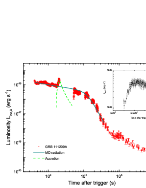
Figure 2: The lightcurve of GRB 111209A. A putative fast raising and exponential decaying profile is used to make a demonstration of accretion profile, and the inset presents a prominent luminosity from dark climb to normal level.

In principle, as the accretion materials close to the surface of the NS, the magnetic field would be dragged by the accretion materials, but the diffusion of magnetic field is also ongoing. If an absolute advantage is occupied by the accretion materials, the magnetic field lines could be buried. Hence, the surface magnetic field of NS would experience a significant decrease, and an empirical behaviour can be written as (Taam & van den Heuvel 1986; Shibazaki et al. 1989; Fu & Li 2013)

$$B(t)=\frac{B_{i}}{1+M_{\rm acc}/M_{c}},$$ (15)

where $B_{i}$ is the initial surface magnetic field strength of NS, $M_{\rm acc}$ the total material that accretes onto magnetar, and the critical mass $M_{c}$ ranges from $10^{-5}$ to $10^{-3}~{}M_{\odot}$. By taking $M_{c}=10^{-3}~{}M_{\odot}$, the surface magnetic field of GRB 111209A should decrease from $0.67\times 10^{15}~{}\rm G$ to $0.04\times 10^{15}~{}\rm G$, and the observed magnetar plateau would experience a significant shrink, for which $L_{\rm dip}\propto B^{2}$. The significant luminosity from dark climb to normal level of the magnetar plateau was observed at $\sim T_{0}+5000~{}\rm s$ and $\sim T_{0}+10000~{}\rm s$, and an inset in Figure 2 gives a demonstration. Whether it can be connected with a re-magnetized process of NS is under debate. The buried magnetic field is suppressed, as time goes by, the NS should be re-magnetized again (Geppert et al. 1999), and the MD radiation would go back to the normal level. The re-magnetized process that based on Ohmic diffusion and the Hall drift should experience thousands years or more (Geppert et al. 1999; Ho 2011; Fu & Li 2013). However, since the magnetar just born thousands of even hundreds of seconds, one of the process that amplifies the initiate magnetic field of a magnetar, convection in the magnetar, cannot be neglected. As estimated by Thompson & Duncan (1993), this process would take about $30~{}\rm s$ only. Hence, it may dominate the re-magnetized process of a buried magnetar scenario. On the other hand, owing to the affection of magnetic field, the funnelled accreting flow is located in the polar region of the magnetized NS (Lamb et al. 1973; Elsner & Lamb 1977; Romanova et al. 2002), the accreting materials onto the centre of the polar cap would also be resisted by the opened magnetic field line (Romanova et al. 2009). Therefore, the re-magnetized process of a portion-buried NS would proceed at the both interior and exterior, and the surface magnetic field should be less affected by interior one. In this scenario, those observed phenomena that the ligtcurve from dark climbs to normal in the magnetar plateau is expected to be understood as the re-magnetized process of a magnetar.

Of course, a significant emission at the period $T_{0}+2000$ to $T_{0}+5000$ $\rm s$ was detected by Konus-Wind (Golenetskii et al. 2011), and a significant transition from bright to dark is also presented. If the suppressing process of magnetic field corresponds to the flare at $T_{0}+2000$, then the emission may be explained as the afterglow component, which is always covered by the magnetar plateau in the observed band of Swift/XRT (e.g., GRB 070110; Troja et al. 2007). If the suppressed magnetic field is caused by the accretion at this phase, it may give a hint that a re-magnetized process can be as short as hundreds of seconds.

Table 1: MD radiation.

GRB	redshift $z$	$\Gamma$	$-\alpha_{2}$	$\tau(z)~{}(\rm\times 10^{4}~{}s)$	$L_{\rm 0,X,iso}~{}(~{}\rm erg~{}s^{-1})$	$B~{}(\rm\times 10^{15}~{}\rm G)$	$P_{0}~{}(\rm ms)$
050730	3.967(1)	1.58	2.77	0.77 $\pm$ 0.05	(2.81 $\pm$ 0.49)$\times 10^{49}$	1.16 $\pm$ 0.13	1.48 $\pm$ 0.14
060607A	3.082(2)	1.55	3.45	1.27 $\pm$ 0.03	(2.35 $\pm$ 0.11)$\times 10^{48}$	1.98 $\pm$ 0.07	3.58 $\pm$ 0.09
111209A	0.677(3)	1.79	4.50	1.23 $\pm$ 0.03	(3.77 $\pm$ 0.07)$\times 10^{48}$	0.67 $\pm$ 0.02	1.85 $\pm$ 0.03
140304A	5.283(4)	1.96	3.50	0.18 $\pm$ 0.04	(4.53 $\pm$ 0.88)$\times 10^{49}$	4.98 $\pm$ 1.19	2.71 $\pm$ 0.40
201221A	5.7(5)	1.45	2.70	1.44 $\pm$ 0.58	(8.94 $\pm$ 0.82)$\times 10^{47}$	4.66 $\pm$ 1.89	7.00 $\pm$ 1.45
060413	…	1.53	3.06	2.51 $\pm$ 0.13	(1.49 $\pm$ 0.11)$\times 10^{48}$	1.47 $\pm$ 0.09	3.45 $\pm$ 0.15
071118	…	1.59	2.20	1.09 $\pm$ 0.15	(9.61 $\pm$ 0.75)$\times 10^{47}$	4.20 $\pm$ 0.60	6.53 $\pm$ 0.51
200306C	…	1.58	2.80	0.43 $\pm$ 0.02	(1.44 $\pm$ 0.10)$\times 10^{48}$	8.67 $\pm$ 0.54	8.47 $\pm$ 0.35

A putative redshift $z=3.74$ based on five unambiguous observations is used to perform the cosmological correction for GRB 060413, GRB 071118, and GRB 200306C. Reference (1) Chen et al. (2005); Rol et al. (2005); Holman et al. (2005); Prochaska et al. (2005); D’Elia et al. (2005); (2) Ledoux et al. (2006); (3) Vreeswijk et al. (2011); (4) de Ugarte Postigo et al. (2014); Jeong et al. (2014); (5) Malesani et al. (2020).

Table 2: The mass trace in each flare.

GRB-flares	$t_{p}$	$E_{\rm fla}$ ($\rm ergs$)	$M_{\rm acc}~{}(M_{\odot})$	$M_{\rm jet}~{}(M_{\odot})$	$M_{\rm disk,loss}~{}(M_{\odot})$
050730-$\rm I$	230	1.11$\times 10^{51}$	7.72$\times 10^{-3}$	9.28$\times 10^{-6}$	8.65$\times 10^{-3}$
050730-$\rm II$	435	3.20$\times 10^{51}$	2.22$\times 10^{-2}$	2.67$\times 10^{-5}$	2.48$\times 10^{-2}$
050730-$\rm III$	677	1.88$\times 10^{51}$	1.31$\times 10^{-2}$	1.57$\times 10^{-5}$	1.46$\times 10^{-2}$
060607A-$\rm I$	95	1.05$\times 10^{51}$	7.30$\times 10^{-3}$	8.78$\times 10^{-6}$	8.18$\times 10^{-3}$
060607A-$\rm II$	263	2.46$\times 10^{51}$	1.70$\times 10^{-2}$	2.05$\times 10^{-5}$	1.91$\times 10^{-2}$
111209A	2027	2.06$\times 10^{51}$	1.43$\times 10^{-2}$	1.72$\times 10^{-5}$	1.60$\times 10^{-2}$
140304A-$\rm I$	327	4.58$\times 10^{51}$	3.17$\times 10^{-2}$	3.81$\times 10^{-5}$	3.55$\times 10^{-2}$
140304A-$\rm II$	820	2.70$\times 10^{51}$	1.87$\times 10^{-2}$	2.25$\times 10^{-5}$	2.10$\times 10^{-2}$
201221A	4152	2.27$\times 10^{51}$	1.58$\times 10^{-2}$	1.89$\times 10^{-5}$	1.76$\times 10^{-2}$
060413	637	1.90$\times 10^{51}$	1.32$\times 10^{-2}$	1.58$\times 10^{-5}$	1.47$\times 10^{-2}$
071118	593	1.63$\times 10^{51}$	1.13$\times 10^{-2}$	1.36$\times 10^{-5}$	1.26$\times 10^{-2}$
200306C	1075	8.67$\times 10^{50}$	6.00$\times 10^{-3}$	7.22$\times 10^{-6}$	6.72$\times 10^{-3}$

The radius and the mass of the magnetar are set as $R=12~{}\rm km$ and $M=1.4~{}M_{\odot}$, respectively. The total mass loss of the disk is marked as $M_{\rm disk,loss}$.

3.3 Observations VS Parameters

The selected cases present a prominent sharp decay ($\alpha_{2}<-2$) following a X-ray plateau ($\alpha_{1}>-0.75$). Ahead of the sharp decay, the remarkable X-ray flares raise upon the X-ray plateau. The lightcurves of the selected cases are shown in Figure 3, and the derived parameters of the MD radiation are organized in Table 1. In these collected cases, five in eight have an unambiguous redshift measurement, four of it are large than 3. The mean redshift of the five cases is $3.74$, it is higher than the mean redshift $z=2.22$ for all of the redshift-measured GRBs that is detected by Swift prominently, this interesting phenomenon was also noticed by Lyons et al. (2010). Here, the mean redshift $z=3.74$ is adopted to achieve the cosmological correction for the rest of the three GRBs. The time average photon index $\Gamma$ of X-ray afterglow for each GRB is listed in column (3), and its median is 1.58. The isotropic X-ray characteristic luminosity of the magnetar spindown process is listed in column (6), and the characteristic spindown time scale in the observer frame is listed in column (5). The surface magnetic field and the initial spin period are presented in column (7) and (8), respectively.

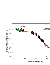
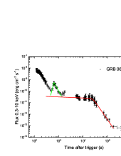
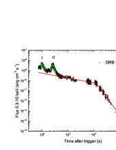
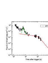
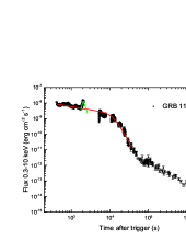
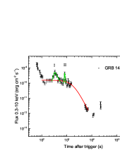
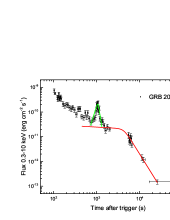
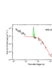
Figure 3: The lightcurves of selected cases that X-ray flares raising upon a magnetar plateau. The magnetar plateaus are exhibited with a red line, and the prominent early flares are marked with green line, the putative profiles are used to give a demonstration for inadequate observations of GRB 111209A and GRB 201221A. Here, if the two or more flares are exhibited in one case, we donate the sign $\rm I$, $\rm II$, and $\rm III$ to distinguish these flares.

There are two or more flares identified in three GRBs (GRB 050730, GRB 060607A, and GRB 140304A), we collect the peak time $t_{p}$ of flares and list them in Table 2 and column (2). In each GRB, the time interval of the first flare to the trigger time almost equal to the time interval of the adjacent two X-ray flares quantitatively. The total mass loading in each flare is listed in Table 2. Its probability distribution is also presented in Figure 4, and the centre of the gaussian profile is $10^{-4.77\pm 0.19}~{}M_{\odot}$.

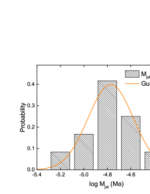
Figure 4: The mass loading distribution of the observed 12 X-ray flares. A gaussian profile is used to show the distribution of mass loading and is exhibited with an orange line.

Following the time interval of the two adjacent flares, the average mass flow rates of the disk for three multi-flare GRBs are estimated to be $3.53\times 10^{-4}~{}M_{\odot}~{}\rm s^{-1}$, $4.23\times 10^{-4}~{}M_{\odot}~{}\rm s^{-1}$, and $4.33\times 10^{-4}~{}M_{\odot}~{}\rm s^{-1}$ for GRB 050730, GRB 060607A, and GRB 140304A, respectively. Therefore, by using Eq. (5), the average sizes of the magnetosphere for corresponding GRBs are $5.01~{}\rm\times 10^{6}cm$, $6.45~{}\rm\times 10^{6}cm$, and $1.09~{}\rm\times 10^{7}cm$, respectively.

4 Conclusions and Discussions

In this paper, we argue that the X-ray flares raising upon a magnetar plateau can be used to connect the accretion process of a magnetar and lead an implication for the existence of a disk surrounding a rapidly rotating and highly magnetized newborn NS. In this scenario, the repeating accretion process is investigated in multi-flare GRB 050730; the accreting induced variation of the magnetic field is discussed in GRB 111209A, and hundreds of seconds re-magnetized process in an accreting magnetar scenario is implied. In the selected cases, three of it show multiple flares in one GRB. In each GRB, the time interval of the first flare to trigger time almost equal to the time interval of the adjacent two X-ray flares quantitatively. In this scenario, by adopting magnetar mass $M=1.4~{}M_{\odot}$ and radius $R=12~{}\rm km$, the average mass flow rates of the disk are $3.53\times 10^{-4}~{}M_{\odot}~{}\rm s^{-1}$, $4.23\times 10^{-4}~{}M_{\odot}~{}\rm s^{-1}$, and $4.33\times 10^{-4}~{}M_{\odot}~{}\rm s^{-1}$ for GRB 050730, GRB 060607A, and GRB 140304A, respectively, and the corresponding average sizes of the magnetosphere of central magnetar are $5.01~{}\rm\times 10^{6}cm$, $6.45~{}\rm\times 10^{6}cm$, and $1.09~{}\rm\times 10^{7}cm$. A sample analysis that contains 8 GRBs within 12 flares shows that the total mass loading in single flare is $\sim 2\times 10^{-5}~{}M_{\odot}$. In the lost mass of a disk, there are about 0.1% portion used to feed the collimated jet. The details are presented in Table 2. Our mass loading result is compatible with the study in Maxham & Zhang (2009). However, since the prominent high redshift ($z>3$ four in five) is given, the selective effect or more deep physical origination may be hinted.

Comparing to stellar fragment fallback determined accretion (e.g., Lin et al. 2021), the MHD instability induced periodic accretion process have a shorter time interval for two successive accretion, for this scenario, the inner disk ram pressure can be released timely. Furthermore, the observed periodic accretion process may imply the disk has reached a quasi-steady state (The disk may erratic when it born in the collapse of a massive star). Just as the simulation in Li et al. (2021), after a significant accretion, the fastness parameter keeps close to 1, the propeller and the accretion effect is comparable. In this scenario, the MHD instability leads the oscillation of disk and triggers the short-duration accretion. Even the periodic accretion process has been studied for several decades (e.g., Balbus & Hawley 1991; Miller & Stone 1997; Ustyugova et al. 2006; Romanova et al. 2009, 2018), a simple analytical formula for each step of the four-step accretion cycle and the jet launch mechanism is hard to be organized still. Hence, the time domain lightcurve is not explored in this work. In the future, by comprehensive consider both the magnetar-disk interaction, and the spin and magnetic field determined jet launch mechanism (e.g., magnetic pressure powered collimated jet; Lovelace et al. 1995; Goodson et al. 1997, 1999), a time domain analytical solution would paint these quasi-steady magnetar-disk system vividly.

There are about $0.01~{}M_{\odot}$ materials needed in a single event, which can be a trouble for a supernova that has exploded more than hundreds or thousands of seconds (Kumar et al. 2008). The magnetosphere collects the fallback materials onto the surrounding disk would boost this process. As a reward, the accompanying disk helps the magnetar to store the rotational energy and returns it when the spin decreases because of an MD radiation or gravitational radiation. This scenario can be used to understand why a high efficiency of converting the rotational energy to the observed X-ray emission was found in Lü & Zhang (2014), by comparing with a modified efficiency format, e.g., $\eta=\int{L_{X}}dt/(E_{rot,NS}+E_{disk})$, where $L_{X}$, $E_{rot,NS}$, $E_{disk}$ are the MD luminosity in X-ray band, the rotational energy of NS, and the energy stored in the surrounding disk, respectively (Zheng et al. 2022, in preparation). Given the two-component outflow scenario, the re-brightening following a sharp decay, e.g., GRB 111209A, can be explained as the catching up of delay conical wind. Considering the evolution of central magnetar, that a small block mass fallback accretion due to the magnetosphere gets a significantly shrinking may also give a reasonable solution for later re-brightening. Therefore, for a later re-brightening following magnetar plateau scenario, at least in some cases, the final stage of the GRB central engine can be an NS rather than a BH (Lin et al. 2020), further deep observations are expected to reveal the mask of the central engine of GRBs.