Distiller: A Systematic Study of Model Distillation Methods in Natural Language Processing

Abstract

Knowledge Distillation (KD) offers a natural way to reduce the latency and memory/energy usage of massive pretrained models that have come to dominate Natural Language Processing (NLP) in recent years. While numerous sophisticated variants of KD algorithms have been proposed for NLP applications, the key factors underpinning the optimal distillation performance are often confounded and remain unclear. We aim to identify how different components in the KD pipeline affect the resulting performance and how much the optimal KD pipeline varies across different datasets/tasks, such as the data augmentation policy, the loss function, and the intermediate representation for transferring the knowledge between teacher and student. To tease apart their effects, we propose Distiller, a meta KD framework that systematically combines a broad range of techniques across different stages of the KD pipeline, which enables us to quantify each component’s contribution. Within Distiller, we unify commonly used objectives for distillation of intermediate representations under a universal mutual information (MI) objective and propose a class of MI-$\alpha$ objective functions with better bias/variance trade-off for estimating the MI between the teacher and the student. On a diverse set of NLP datasets, the best Distiller configurations are identified via large-scale hyper-parameter optimization. Our experiments reveal the following: 1) the approach used to distill the intermediate representations is the most important factor in KD performance, 2) among different objectives for intermediate distillation, MI-$\alpha$ performs the best, and 3) data augmentation provides a large boost for small training datasets or small student networks. Moreover, we find that different datasets/tasks prefer different KD algorithms, and thus propose a simple AutoDistiller algorithm that can recommend a good KD pipeline for a new dataset.

1 Introduction

Recent advancements in Natural Language Processing (NLP) such as BERT Devlin et al. (2019), RoBERTa Liu et al. (2019), and ELECTRA Clark et al. (2020) have demonstrated the effectiveness of Transformer models in generating transferable language representations. Pretraining over a massive unlabeled corpus and then fine-tuning over labeled data for the task of interest has become the state-of-the-art paradigm for solving diverse NLP problems ranging from sentence classification to question answering Raffel et al. (2019). Scaling up the size of these networks has led to rapid NLP improvements. However, these improvements have come at the expense of significant increase of memory for their many parameters and compute to produce predictions Brown et al. (2020); Kaplan et al. (2020). This prevents these models from being deployed on resource-constrained devices such as smart phones and browsers, or for latency-constrained applications such as click-through-rate prediction. There is great demand for models that are smaller in size, yet still retain similar accuracy as those having a large number of parameters.

To reduce the model size while preserving accuracy, various model compression techniques have been proposed such as: pruning, quantization, and Knowledge Distillation (KD) Gupta and Agrawal (2020). Among these methods, task-aware KD is a popular and particularly promising approach for compressing Transformer-based models Gupta and Agrawal (2020). The general idea is to first fine-tune a large model (namely the teacher model) based on the task’s labeled data, and then train a separate network that has significantly fewer parameters (namely the student model) than the original model to mimic the predictions of the original large model. A large number of task-aware KD algorithms have been proposed in the NLP regime, e.g., DistillBERT Sanh et al. (2019), BERT-PKD Sun et al. (2019), BERT-EMD Li et al. (2020), TinyBERT Jiao et al. (2020), DynaBERT Hou et al. (2020), and AdaBERT Chen et al. (2020), some of which can compress the teacher network by 10$\times$ without significant accuracy loss on certain datasets.

Innovations in KD for NLP generally involve improvements in one of the following aspects: 1) the loss function for gauging the discrepancy between student and teacher predictions Kim et al. (2021), 2) the method for transferring intermediate network representations between teacher and student Sun et al. (2019); Li et al. (2020); Yang et al. (2021), 3) the use of data augmentation during student training Jiao et al. (2020), and 4) multiple stages of distillation Chen et al. (2020); Mirzadeh et al. (2020). Many research proposals have simultaneously introduced new variations of more than one of these components, which confounds the impact of each component on the final performance of the distillation algorithm. In addition, it is often unclear whether a proposed distillation pipeline will generalize to a new dataset or task, making automated KD challenging. For example, MixKD Liang et al. (2021) has only been evaluated on classification problems and it is unclear if the method will be effective for question answering.

To understand the importance of different components in KD, we undertake a systematic study of KD algorithms in NLP. Our study is conducted using a meta-distillation pipeline we call Distiller that contains multiple configurable components. All candidate algorithms in the search space of Distiller work for two types of NLP tasks: text classification and sentence tagging. Distiller unifies existing techniques for knowledge transfer from intermediate layers of the teacher network to the student network (i.e. intermediate distillation) as special cases of maximizing (bounds on) the Mutual Information (MI) between teacher and student representations. Based on this unification and recent progress in variational bounds of MI Poole et al. (2019), we propose a new intermediate distillation objective called MI-$\alpha$ that uses a scalar $\alpha$ to control the bias-variance trade-off of MI estimation. Including MI-$\alpha$ in the search space of Distiller, we run extensive hyper-parameter tuning algorithms to search for the best Distiller-configuration choices over GLUE Wang et al. (2019b) and SQuAD Rajpurkar et al. (2016). This search helps us identify the best distillation pipelines and understand what impact different KD modules have on student performance in NLP. Using the observations of this large-scale study, we train a AutoDistiller model to predict the distillation ratio, which is defined as the fraction of the teacher’s performance achieved by the student, based on KD pipeline choices and characteristics of a dataset. Leave-one-out cross validation evaluation of AutoDistiller demonstrates that it is able to reliably prioritize high-performing KD configurations in most folds, and is able to suggest good distillation pipelines on two new datasets.

The main contributions of this work include:

• The meta KD pipeline Distiller used to systematically study the impact of different components in KD, including the: 1) data augmentation policy, 2) loss function for transferring intermediate representations, 3) layer mapping strategies for intermediate representations, 4) loss function for transferring outputs, as well as what role the task/dataset play.

• Unification of existing objectives for distilling intermediate representations as instances of maximizing bounds of the mutual information between teacher and student representations. This leads us to propose the MI-$\alpha$ objective that outperforms the existing objectives.

• Using the results collected from our systematic Distiller study, we fit a model that automatically predicts the best distillation strategy for a new dataset. On a never-seen dataset “BoolQ”Wang et al. (2019a), predicted strategies achieve $1.002$ distillation ratios (fraction of the student’s and the teacher’s performance) on average, outperforming random selected strategies with mean of $0.960$. To the best of our knowledge, this is the first attempt towards automated KD in NLP.

2 Related Work

Knowledge Distillation.

The general KD framework was popularized by Buciluǎ et al. (2006); Hinton et al. (2014), aiming to transfer knowledge from an accurate but cumbersome teacher model to a compact student model by matching the class probabilities produced by the teacher and the student. Focusing on AutoML settings with tabular data, Fakoor et al. (2020) proposed a general KD algorithm for different classical ML models and ensembles thereof. Also hoping to identify good choices in the KD pipeline like our work, Kim et al. (2021) compared Kullback-Leibler divergence and mean squared error objectives in KD for image classification models, finding that mean squared error performs better.

Recent KD research in the domain of NLP has investigated how to efficiently transfer knowledge from pretrained Transformer models. Sun et al. (2019) proposed BERT-PKD that transfers the knowledge from both the final layer and intermediate layers of the teacher network. Jiao et al. (2020) proposed the TinyBERT model that first distills the general knowledge of the teacher by minimizing the Masked Language Model (MLM) objective Devlin et al. (2019), with subsequent task-specific distillation. Li et al. (2020) proposed a many-to-many layer mapping function leveraging the Earth Mover’s Distance to transfer intermediate knowledge. Our paper differs from the existing work in that we provide a systematic analysis of the different components in single-stage task-aware KD algorithms in NLP and propose the first automated KD algorithm in this area.

Mutual Information Estimation.

Mutual Information (MI) measures the degree of statistical dependence between random variables. Given random variables $A$ and $B$, the MI between them, $I(A,B)$, can be understood as how much knowing $A$ will reduce the uncertainty of $B$ or vice versa. For distributions that do not have analytical forms, maximizing MI directly is often intractable. To overcome this difficulty, recent work resorts to variational bounds Donsker and Varadhan (1975); Blei et al. (2017); Nguyen et al. (2010) and deep learning Oord et al. (2018) to estimate MI. These works utilize flexible parametric distributions or critics that are parameterized neural networks (NNs) to approximate unknown densities that appear in MI calcuations. Poole et al. (2019) provides a review of existing MI estimators and proposes novel bounds that trade-off bias and variance. Kong et al. (2020) unified language representation learning objective functions from the MI maximization perspective.

Data Augmentation in NLP.

Data Augmentation (DA) is an effective technique for improving the accuracy of text classification models Wei and Zou (2019) and has also been shown to boost the performance of KD for NLP algorithms Jiao et al. (2020) as well as KD in models for tabular data Fakoor et al. (2020). Wei and Zou (2019) proposed the Easy Data Augmentation (EDA) technique that randomly replaces synonyms, inserts, swaps and deletes characters in the sentence. Jiao et al. (2020) proposed to utilize the pretrained BERT model and GloVe word embeddings Pennington et al. (2014) to augment the input sentence via random word-level replacement. MixKD Liang et al. (2021) adopts mixup Zhang et al. (2018) and backtranslation Edunov et al. (2018) in augmenting the text data to boost the performance of sentence classification models. Unlike these papers, we propose a novel search space for DA policies that supports stacking elementary augmentation operations such as EDA, mixup, and backtranslation. Thus, our considered DA module is similar to AutoAugment Cubuk et al. (2019), except it is used for KD in NLP with different elementary operators.

3 Methodology

Our study is structured around a configurable meta-distillation pipeline called Distiller. Distiller contains four configurable components, namely: a data augmentation policy $a(\cdot,\cdot)$, a layer mapping configuration of intermediate distillation $\{m_{i,j}\}$, an intermediate distillation objective $l^{\text{inter}}(\cdot,\cdot)$, and a prediction layer distillation objective $l^{\text{pred}}(\cdot,\cdot)$. Assume the teacher network $f^{T}$ has $M$ layers and the student network $f^{S}$ has $N$ layers. Then for a given data/label pair $(x,y)$ sampled from the dataset $\mathcal{D}$, the student acquires knowledge from the teacher by minimizing the following objective:

$$\mathcal{L} =\mathbb{E}_{\hat{x},\hat{y}\sim a(x,y);x,y\sim\mathcal{D}}\sum_{i=1}^{M}\sum_{j=1}^{N}m_{i,j}l_{i,j}^{\text{inter}}(H_{i}^{\text{T}},H_{j}^{\text{S}})$$ (1)

$$+\beta_{1}l^{\text{pred}}(f^{T}(x),f^{S}(x))+\gamma_{1}l^{\text{pred}}(y,f^{S}(x))$$

$$+\beta_{2}l^{\text{pred}}(f^{T}(\hat{x}),f^{S}(\hat{x}))+\gamma_{2}l^{\text{pred}}(\hat{y},f^{S}(\hat{x})),$$

Here $m_{i,j}\in[0,1]$ represents the layer mapping weight between the $i$-th teacher layer and $j$-th student layer, $H_{i}^{\text{T}},H_{j}^{\text{S}}$ are the $i$-th and the $j$-th hidden states of the teacher and the student (i.e. their intermediate representations at layers $i$ and $j$), $\beta_{1}$, $\beta_{2}$ control the strength of distilling from class probabilities produced by the teacher, and $\gamma_{1}$ and $\gamma_{2}$ control the strength of learning from ground truth data ($x,y$) and synthesized (augmented) data ($\hat{x},\hat{y}$). In Appendix, we illustrated how previous model distillation algorithms Jiao et al. (2020); Li et al. (2020); Liang et al. (2021) can be encompassed in the Distiller framework.

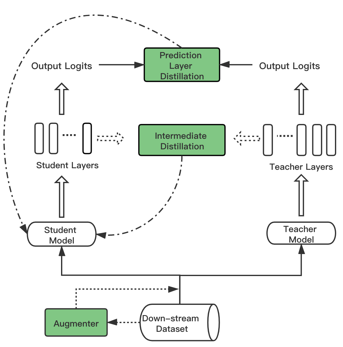
Figure 1: Overview of the Distiller pipeline. All configurable components are colored.

3.1 Data Augmentation Policy

Params: A sequence of elementary data augmentation operations $\mathcal{G}$, $\forall\mathcal{G}_{j}\in\{\textit{CA},\textit{RA},\textit{BT},\textit{Mixup}\}$.

Input: Training Dataset $\mathcal{D}_{\text{train}}$

Output: Augmented dataset $\mathcal{D}_{\text{synthesize}}$

1 Initialize $\mathcal{D}_{\text{synthesize}}\leftarrow\{\}$

2 foreach $\{x_{i},y_{i}\}\in\mathcal{D}_{\text{train}}$ do

3       for j $\leftarrow$ 1 to len($\mathcal{G}$) do

4             $\hat{x}_{i},\hat{y}_{i}=\mathcal{G}_{j}(x_{i},y_{i})$;

5             $x_{i},y_{i}\leftarrow\hat{x}_{i},\hat{y}_{i}$;

6            

7       end for

8      $\mathcal{D}_{\text{synthesize}}\leftarrow\mathcal{D}_{\text{synthesize}}\cup\{x_{i},y_{i}\}$

9 end foreach

Algorithm 1 Data Augmentation Policy

A key challenge is the limited data available to train students in KD. This can be mitigated via Data Augmentation (DA) to generate additional data samples. Unlike in supervised learning, where labels for synthetic augmented data may be unclear unless the augmentation is limited to truly benign perturbations, the labels for augmented data in KD are simply provided by the teacher which allows for more aggressive augmentation Fakoor et al. (2020). Denoting the set of training samples of the down-stream task as $\mathcal{D}_{\text{train}}$, the augmenter $a(\cdot,\cdot)$ will stretch the distribution from $E_{x,y\sim{\mathcal{D}_{\text{train}}}}$ to $E_{\hat{x},\hat{y}\sim{a(x,y)},x,y\sim{\mathcal{D}_{\text{train}}}}$. We consider various elementary DA operations including: 1) MLM-based contextual augmentation (CA) , 2) random augmentation (RA), 3) backtranslation (BT) and 4) mixup. The search space of possible augmentations in Distiller is constructed by stacking these four elementary operations in an arbitrary order, as detailed in Algorithm 1.

For contextual augmentation, we use the pretrained BERT model to do word level replacement by filling in randomly masked tokens. As in EDA Wei and Zou (2019), our random augmentation randomly swaps words in the sentence or replaces words with their synonyms. For backtranslation, we translate the sentence from one language (in this paper, English) to another language (in this paper, German) and then translate it back. Additionally, mixup can be used to synthesize augmented training samples. First proposed for image classification Zhang et al. (2018), mixup constructs a synthetic training example via the weighted average of two samples (including the labels) drawn at random from the training data. To use it in NLP, Guo et al. (2019); Liang et al. (2021) applied mixup on the word embeddings at each sentence position $x_{i,t}$ with $\lambda\in[0,1]$ as the mixing-ratio for a particular pair of examples $x_{i},x_{j}$:

$$\hat{x}_{i,t}=\lambda x_{i,t}+(1-\lambda)x_{j,t},~{}\hat{y}_{i}=\lambda y_{i}+(1-\lambda)y_{j},$$

Here $\lambda$ is typically randomly drawn from a Uniform or Beta distribution for each pair, $y_{i},y_{j}$ are labels in one-hot vector format, and $(\hat{x}_{i},\hat{y}_{i})$ denotes the new augmented sample. To apply mixup for sentence tagging tasks, in which each token has its own label, we propose calculating the weighted combination of the ground-truth target at each location $t$ as the new target:

$$\hat{x}_{i,t}=\lambda x_{i,t}+(1-\lambda)x_{j,t},~{}\hat{y}_{i,t}=\lambda y_{i,t}+(1-\lambda)y_{j,t},\$$

3.2 Prediction Layer Distillation

In traditional KD, the student network learns from the output logits of the teacher network, adopting these as soft labels for the student’s training data Hinton et al. (2014). Here we penalize the discrepancy between the outputs of student vs. teacher via:

$$\mathcal{L}_{\text{pred}}=l^{\text{pred}}(f^{T}(x),f^{S}(x)),$$ (2)

where $l^{\text{pred}}(\cdot,\cdot)$ is the KD loss component whose search space in this work includes either: softmax Cross-Entropy (CE) or Mean Squared Error (MSE).

3.3 Intermediate Representation Distillation

To ensure knowledge is sufficiently transferred, we can allow the student to learn from intermediate layers of the teacher rather than only the latter’s output predictions by minimizing discrepancies between selected layers from the teacher and the student. These high-dimensional intermediate layer representations constitute a much richer information-dense signal than is available in the low-dimensional predictions from the output layer. As teacher and student usually have different number of layers and hidden-state dimensionalities, it is not clear how to map teacher layers to student layers ($m_{i,j}$) and how to measure the discrepancy between their hidden states ($l_{i,j}^{\text{inter}}$). Previous works proposed various discrepancy measures (or loss functions) for intermediate distillation, including: Cross-Entropy (CE), Mean Squared Error (MSE), L2 distance, Cosine Similarity (Cos), and Patient Knowledge Distillation (PKD) Sun et al. (2019). For these objectives, we establish the following result (the proof is relegated to the Appendix).

Theorem 3.1

Minimizing MSE, L2, or PKD loss, and maximizing cosine similarity between two random variables $X$,$Y$ are equivalent to maximizing lower bounds of the mutual information $I(X;Y)$.

In our KD setting, $X$ and $Y$ correspond to the hidden state representations of our student and teacher model (for random training examples), respectively. Inspired by this result, we can use any lower bounds of MI as an intermediate objective function in KD. In particular, we consider the multisample MI lower bound of Poole et al. (2019), which estimates $I(X;Y)$ given the sample $x,y$ from $p(x,y)$ and another $K$ additional IID samples $z_{1:{K}}$ that are drawn from a distribution independent from $X$ and $Y$:

$$I(X;Y) \geq E_{p(x,z_{1:{K}})p(y|x)}\left[\log\frac{e^{f(x,y)}}{\alpha m(y;x,z_{1:{K}})+(1-\alpha)q(y)}\right]$$

$$-E_{p(x,z_{1:{K}})p(y)}\left[\log\frac{e^{f(x,y)}}{\alpha m(y;x,z_{1:{K}})+(1-\alpha)q(y)}\right]+1$$

$$\triangleq I_{\alpha}.$$ (3)

In $I_{\alpha}$, $f(\cdot,\cdot)$ and $q(\cdot)$ are critic functions for approximating unknown densities and $m(\cdot,\cdot)$ is a Monte-Carlo estimate of the partition function that appears in MI calculations. Typically, the space $z$ and the sample $x,y$ are from the same minibatch while training, that is $K+1$ equals to the minibatch size. $I_{\alpha}$ can flexibly trade off bias and variance, since increasing $\alpha\in[0,1]$ will reduce the variance of the estimator while increasing its bias. We propose to use $I_{\alpha}$ as an objective for intermediate distillation and call it MI-$\alpha$. Our implementation leverages a Transformer encoder Vaswani et al. (2017) to learn $f(\cdot,\cdot)$ and $q(\cdot)$. To our knowledge, this is the first attempt to utilize complex NN architectures for critic functions in MI estimation; typically only shallow multilayer perceptrons (MLPs) are used Tschannen et al. (2020). Our experiments (Table 4 in Appendix) reveal that Transformer produces a better critic function than MLP.

Note that for intermediate distillation, objectives like MSE attempt to ensure the teacher and student representations take matching values, whereas objectives like MI (and tighter bounds thereof) merely attempt to ensure the information in the teacher representation is also captured in the student representation. The latter aim is conceptually better suited for KD, particularly in settings where the student’s architecture differs from the teacher (e.g. it is more compact), in which case forcing intermediate student representations to take the exact same values as teacher representations seems overly stringent and unnecessary for a good student (it may even be harmful for tiny student networks that lack the capacity to learn the same function composition used by the teacher). We emphasize that a high MI between student and teacher representations suffices for the teacher’s prediction to be approximately recovered from the student’s intermediate representation (assuming the teacher uses deterministic output layers as is standard in today’s NLP models). Given that high MI suffices for the student to match the teacher, we expect tighter MI bounds like MI-$\alpha$ can outperform looser bounds like MSE that impose additional requirements on the student’s intermediate representations beyond just their information content.

3.3.1 Layer Mapping Strategy

We investigate three intermediate layer mapping strategies: 1) Skip: the student learns from every $\lfloor M/N\rfloor$ layer of the teacher, i.e., $m_{i,j}=1$ when $j=i\times\lfloor M/N\rfloor$; 2) Last: the student learns from the last $k$ layers of the teacher, i.e., $m_{i,j}=1$ when $j=i+M-N$; and 3) EMD: a many-to-many learned layer mapping strategy Li et al. (2020) based on Earth Mover’s Distance. In the Distiller pipeline, the intermediate loss with EMD mapping can be denoted as:

$$\mathcal{L}_{\text{EMD}}(H^{S}_{1:N},H^{T}_{1:M})=\frac{\sum_{i=1}^{M}\sum_{j=1}^{N}w_{i,j}^{H}d_{i,j}^{H}}{\sum_{i=1}^{M}\sum_{j=1}^{N}w_{i,j}^{H}},$$ (4)

where $D^{H}=[d_{i,j}^{H}]$ is a distance matrix representing the cost of transferring the hidden states knowledge from $H^{T}$ to $H^{S}$. And $W^{H}=[w_{i,j}^{H}]$ is the mapping flow matrix which is learned by minimizing the cumulative cost required to transfer knowledge from $H^{T}$ to $H^{S}$. In Distiller, the distance matrix is calculated via intermediate objective function: $d_{i,j}^{H}=l^{\text{inter}}(H_{i}^{S},H_{j}^{T})$.

3.4 AutoDistiller

Our experiments indicate that the best distillation algorithm varies among datasets/tasks (see in particular the top-5 configurations listed in Table 9 in Appendix). This inspires us to train a prediction model that recommends a good KD pipeline given a dataset. To represent the distillation performance across datasets which are evaluated on different metrics, we define distillation ratio as the fraction of the teacher’s performance achieved by the student and use it as a general score for distillation performance. Then the prediction model can be trained to predict the distillation ratio based on features of the dataset/task as well as the features of each candidate distillation pipeline. Here we train our AutoDistiller performance prediction model via AutoGluon-Tabular, a simple AutoML tool for supervised learning Erickson et al. (2020). To the best of our knowledge, our proposed method is the first attempt towards automated KD in NLP.

4 Experimental Setup

To study the importance of each component described in the previous section, we randomly sample Distiller configurations in the designed search space while fixing the optimizer and other unrelated hyper-parameters. We apply each sampled distillation configuration on a diverse set of NLP tasks and different teacher/student architectures. All experiments are evaluated on GLUE Wang et al. (2019b) and SQuAD v1.1 Rajpurkar et al. (2016) that contain classification, regression, and sentence tagging tasks. Here, we view the question answering problem in SQuAD v1.1 as finding the correct answer span from the given context, which is essentially a sentence tagging task. We adopt the same metrics for these tasks as in the original papers Wang et al. (2019b); Rajpurkar et al. (2016).

Since Turc et al. (2019) finds initializing students with pretrained weights is better for distillation, we initialize student models with either weights obtained from task-agnostic distillation Jiao et al. (2020) or pretrained from scratch Turc et al. (2019). Three different pretrained models $\text{BERT}_{\text{BASE}}$ Devlin et al. (2019), $\text{RoBERTa}_{\text{LARGE}}$ Liu et al. (2019) and $\text{ELECTRA}_{\text{LARGE}}$ Clark et al. (2020) are considered as teacher models in our experiments after task-specific fine-tuning. As student models, we consider options like $\text{TinyBERT}_{4}$, $\text{ELECTRA}_{\text{SMALL}}$, as well as other models detailed in Table 6 in Appendix.

Existing implementations of data augmentation in KD for NLP generally first generate an augmented dataset that is $K$ times larger than the original one and then apply the distillation algorithm over the augmented dataset. Such implementation separates the process of DA from KD, leading to a time/storage-consuming and inflexible KD pipeline. In Distiller, we instead apply DA dynamically during training. In addition, we use the teacher network to compute the soft label $\hat{y}$ assigned to any augmented sample $\hat{x}$.

To analyze the importance of different components in Distiller, we adopted fANOVA Hutter et al. (2014), an algorithm for quantifying the importance of individual hyper-parameters as well as their interactions in determining down-stream performance. We use fANOVA to evaluate the importance of the four components in Distiller as well as their pairwise combinations: data augmentation, intermediate distillation objective, layer mapping strategy, and prediction layer distillation objective.

Table 1: Comparison of evaluation results on GLUE test set. $\text{BERT}_{\text{BASE}}$ (G) and $\text{BERT}_{\text{BASE}}$ (T) indicate the fine-tuned $\text{BERT}_{\text{BASE}}$ from Devlin et al. (2019) and the teacher model trained by ourselves, respectively. $\text{BERT-EMD}_{4}$ and MI-$\alpha$ are both initialized from $\text{TinyBERT}_{4}$, the difference is that $\text{BERT-EMD}_{4}$ is trained with “EMD” as intermediate layer mapping strategy and MSE as intermediate loss, our MI-$\alpha$ model is trained with “Skip” as intermediate layer mapping strategy and MI-$\alpha$ as intermediate loss.

Model	#Params	MNLI-m	MNLI-mm	QQP	QNLI	SST-2	CoLA	MRPC	RTE	STS-B	AVG
		(393k)	(393k)	(364k)	(108k)	(67k)	(8.5k)	(3.5k)	(2.5k)	(5.7k)
$\text{BERT}_{\text{BASE}}$ (G)	110M	84.6	83.4	71.2	90.5	93.5	52.1	88.9	66.4	85.8	79.6
$\text{BERT}_{\text{BASE}}$ (T)	110M	84.5	83.6	71.7	90.9	93.4	49.3	87.0	67.3	84.7	79.2
$\text{BERT-PKD}_{4}$ Sun et al. (2019)	52M	79.9	79.3	70.2	85.1	89.4	24.8	82.6	62.3	82.3	72.9
$\text{BERT-EMD}_{4}$ Li et al. (2020)	14M	82.1	80.6	69.3	87.2	91.0	25.6	87.6	66.2	82.3	74.7
MI-$\alpha$ ($\alpha=0.9$, ours)	14M	81.9	80.6	69.8	87.4	91.5	25.9	87.0	67.4	84.0	75.1

5 Experimental Results

Under the previously described experimental setup, we conducted a random search over Distiller configurations on each dataset and collected more than 1300 data points in total. Each collected data point contains a particular Distiller configuration, the dataset/task, the teacher/student architectures, and the final performance of the student model. Analyzing the data reveals three major findings:

1. Design of the intermediate distillation module is the most important choice among all factors studied in Distiller.

2. Among different loss functions for intermediate distillation, MI-$\alpha$ performs the best.

3. DA provides a large boost when the dataset or the student model is small.

Additionally, we observe that the best distillation policy varies among datasets/tasks as shown in Table 9 in Appendix. Thus we train a meta-learning model, AutoDistiller, that can recommend a good distillation policy on any new NLP dataset based on which configurations tended to work well for similar datasets in our study.

5.1 Importance of Distiller Components

Figure 2 illustrates that the objective function for intermediate distillation $l^{\text{pred}}$ has the highest individual importance out of all components in Distiller, and the combination of the intermediate distillation objective and layer mapping strategy has the highest joint importance. Thus these are the components one should most critically focus on when selecting a particular KD pipeline. One hypothetical explanation is that the teacher can provide token-level supervision to the student via intermediate distillation, which can better guide the learning process of the student. Our finding is also consistent with the previous observations Sun et al. (2019); Li et al. (2020).

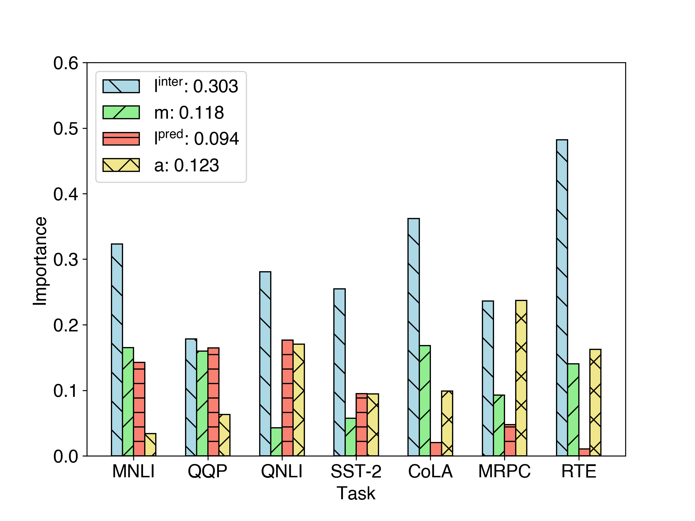
Figure 2: As assessed via fANOVA, we report the individual importance of the four Distiller components in this figure and importance of interactions between any two of the four components in Figure 6 in Appendix. Four components are: $l^{\text{inter}}$ for intermediate distillation objective, $l^{\text{pred}}$ for prediction layer objective, $a$ for data augmentation and $m$ for layer mapping strategy. Average importance for each component (across tasks) is listed in the legend.

5.2 MI-$\alpha$ for Intermediate Distillation

We submitted our MI-$\alpha$ model predictions to the official GLUE leaderboard to obtain test set results and also report the average scores over all tasks (the “AVG” column) as summarized in Table 1. The results show that the student model distilled via the MI-$\alpha$ objective function outperforms previous student models distilled via MSE or PKD loss. To further verify the effectiveness of MI-$\alpha$, we compare how different choices of $l^{\text{inter}}$ affect the distillation performance. In detail, we first pick the top 5 best Distiller strategies according to the evaluation scores for every task and then count how many times each intermediate objective function appears in these strategies. Figure 3 shows that MI-$\alpha$ appears more frequently than all other objectives on both classification and regression tasks. And the results for SQuAD v1.1 in Table 2 indicate the MI-$\alpha$ also works well for sentence tagging.

Table 2: Ablation study of distillation performance on SQuAD v1.1 dev set. The first line shows the performance of the $\text{BERT}_{\text{BASE}}$ teacher. $\text{ELECTRA}_{\text{SMALL}}$, $\text{TinyBERT}_{6}$ and $\text{TinyBERT}_{4}$ are three student networks. $\text{ELECTRA}_{\text{SMALL}}$ (FT) means to fine-tune without KD. ${\text{TinyBERT}_{6}}^{\dagger}$ and ${\text{TinyBERT}_{4}}^{\dagger}$ are results obtained from Jiao et al. (2020). Models that end with “(MSE)” are trained with the MSE loss. “+ MI-$\alpha$” means to distill the student with MI-$\alpha$ ($\alpha$=0.9) as the intermediate loss function. “+ mixup” means to further apply the mixup augmentation.

Model	SQuAD v1.1
	EM	F1
$\text{BERT}_{\text{BASE}}$ (T)	80.9	88.2
$\text{ELECTRA}_{\text{SMALL}}$ (FT)	75.3	83.5
$\text{ELECTRA}_{\text{SMALL}}$ (MSE)	79.2	86.8
+ MI-$\alpha$	79.0	86.8
+ mixup, MSE	80.1	87.4
+ mixup, MI-$\alpha$	80.2	87.6
${\text{TinyBERT}_{6}}^{\dagger}$ Jiao et al. (2020)	79.7	87.5
$\text{TinyBERT}_{6}$ (MSE)	77.8	85.5
+ MI-$\alpha$	80.0	87.8
+ mixup, MSE	78.6	86.2
+ mixup, MI-$\alpha$	81.1	88.6
${\text{TinyBERT}_{4}}^{\dagger}$ Jiao et al. (2020)	72.7	82.1
$\text{TinyBERT}_{4}$ (MSE)	72.7	81.7
+ MI-$\alpha$	71.7	81.2
+ mixup, MSE	72.4	81.4
+ mixup, MI-$\alpha$	71.9	82.5

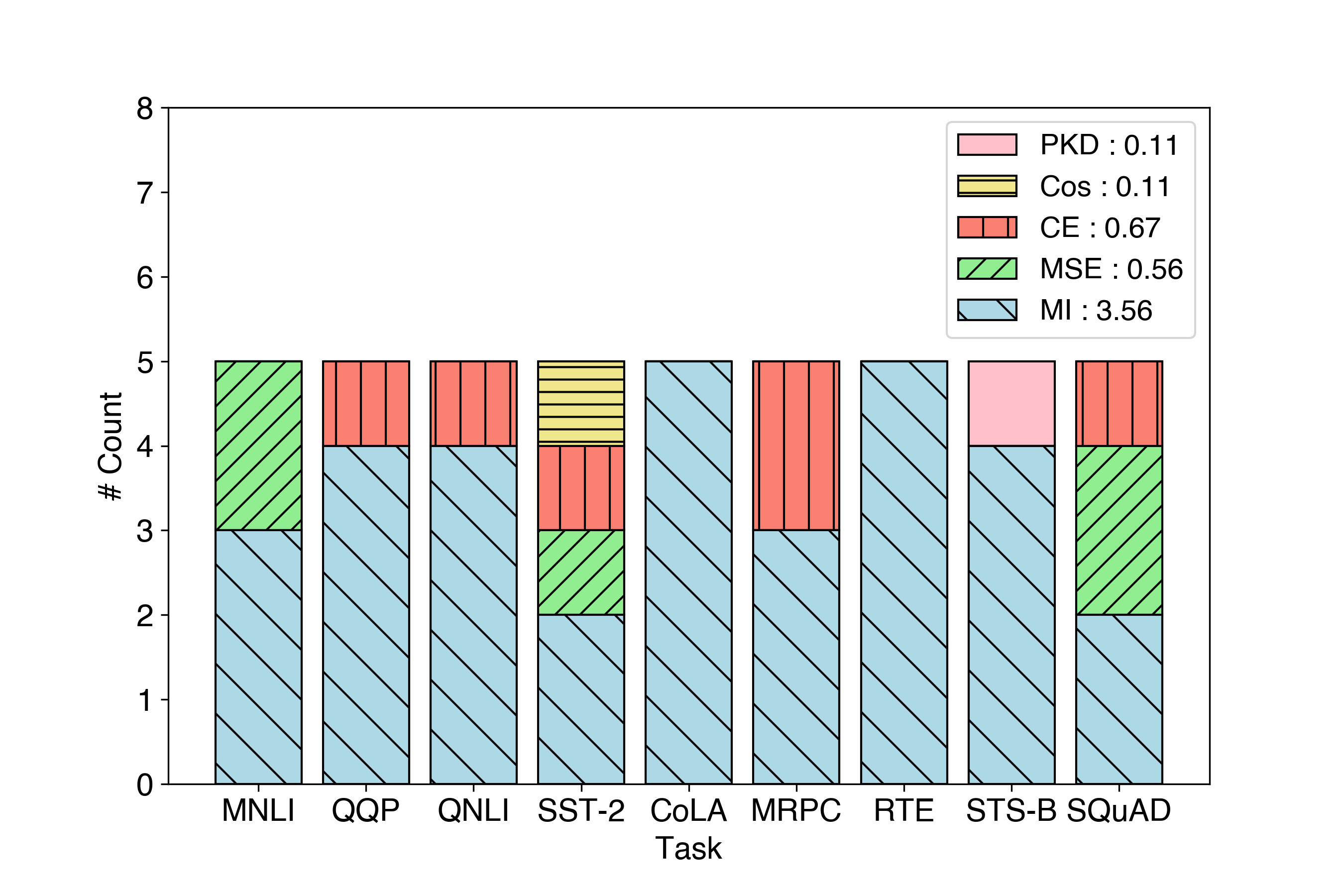
Figure 3: Intermediate objective functions used in the top-5 performing KD configurations on each dataset. The average count of each objective function is listed in the legend. Configurations are detailed in Appendix.

5.3 Benefits of Data Augmentation

Data augmentation in KD provides the student additional opportunities to learn from the teacher, especially for datasets of limited size. Thus, our experiments investigate the effect of DA on four data-limited tasks: CoLA, MRPC, RTE and STS-B. We also study whether students with different architectures/sizes benefit dissimilarly from DA. Table 3 demonstrates that DA generally provides a boost to student performance and is especially beneficial for small models ($\text{BERT}_{\text{MINI}}$ and $\text{BERT}_{\text{TINY}}$).

Table 3: Student performance with(out) augmentation (augmenter initialized as CA+RA+mixup). We report the relative improvement for rows starting with “+ aug”.

Model	#Params	CoLA	MRPC	RTE	STS-B	AVG
		mcc	f1/acc	acc	spearman/pearson
$\text{BERT}_{\text{BASE}}~{}\text{(T)}$	110M	55.0	89.6/85.0	65.0	88.4/88.6	78.6
$\text{TinyBERT}_{\text{6}}$	67M	51.3	92.5/89.7	75.5	89.6/89.8	81.4
+ aug		+0.1	-1.1/-1.8	-3.3	+0.2/+0.2	-1.0
$\text{BERT}_{\text{MEDIUM}}$	41M	44.1	89.3/84.8	65.3	88.3/88.6	76.7
+ aug		+5.3	-0.4/-0.7	+4.4	+0.6/+0.5	+1.6
$\text{BERT}_{\text{SMALL}}$	29M	37.4	86.8/80.6	64.6	87.7/88.0	74.2
+ aug		+5.0	+0.1/+0.8	+0.4	+0.3/+0.2	+1.1
$\text{TinyBERT}_{\text{4}}$	14M	23.6	88.9/83.8	67.1	88.0/88.1	73.3
+ aug		+7.9	+0.3/+0.0	+2.2	+0.7/+0.7	+2.0
$\text{ELECTRA}_{\text{SMALL}}$	14M	42.8	88.3/83.8	66.4	87.4/87.5	76.0
+ aug		+16.2	+3.4/+3.7	+1.8	+1.0/+1.0	+4.5
$\text{BERT}_{\text{MINI}}$	11M	11.2	86.1/80.1	62.8	87.1/87.2	69.1
+ aug		+23.2	+0.0/-0.1	+3.3	+0.2/+0.0	+4.4
$\text{BERT}_{\text{TINY}}$	4M	6.0	83.2/73.3	60.0	84.0/83.6	65.0
+ aug		+6.6	+1.7/+3.7	+4.3	+0.1/+0.7	+2.9

5.4 Performance of AutoDistiller

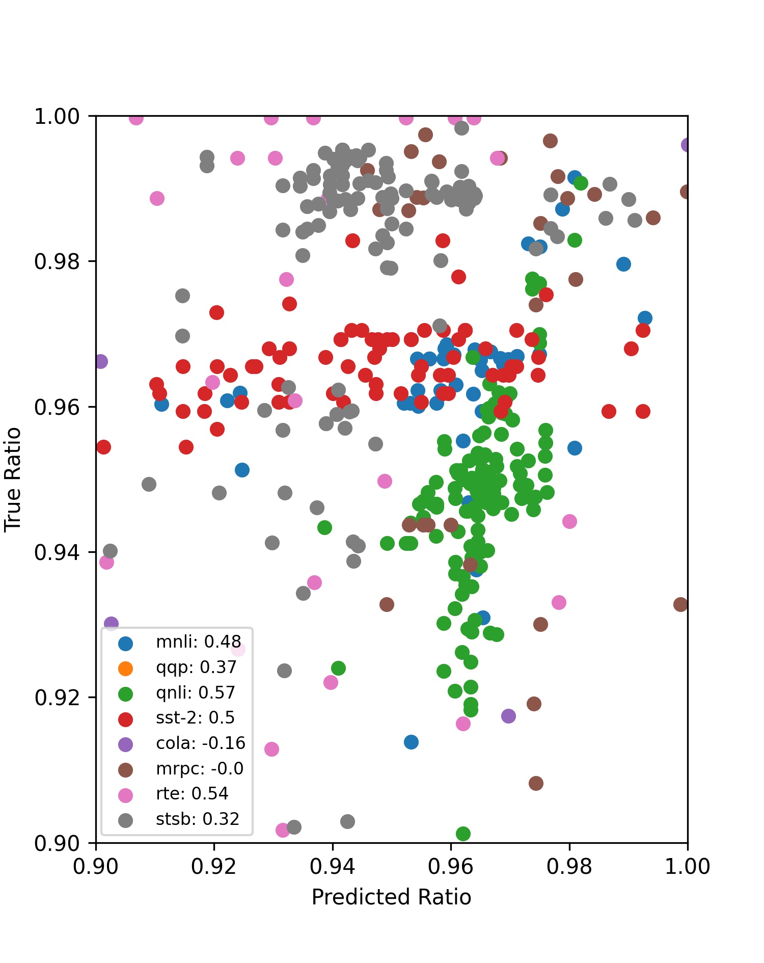
Figure 5: Evaluating held-out AutoDistiller predictions on GLUE via leave-one-out estimates. We use dataset-level cross-validation that holds out each GLUE dataset from AutoDistiller training. For each held-out dataset, the legend lists Spearman’s rank correlation between the predicted vs. actual distillation ratio across different KD pipelines. The average Spearman’s rank correlation value across the 8 datasets is 0.33.

Recall that we train our AutoDistiller performance prediction model on the previously collected experimental results via AutoGluon-Tabular. Once trained, AutoDistiller can recommend distillation pipelines for any down-stream dataset/task by fixing the dataset/task features and searching for configurations that maximize the predicted distillation ratio. AutoDistiller operates on features that represent the dataset domain, the task type, and the task complexity, which are detailed in Appendix. We evaluate the performance of AutoDistiller on the 8 GLUE datasets via a leave-one-dataset-out cross-validation protocol. Figure 5 in Appendix shows that AutoDistiller achieves positive Spearman’s correlation coefficients for most datasets.

Finally, we applied AutoDistiller on two unseen datasets “BoolQ” Wang et al. (2019a) and “cloth” Shi et al. (2021) not considered in our previous experiments. We compared the distillation ratio obtained by each of the top-$N$ strategies suggested by AutoDistiller with the distillation ratio from each of $N$ randomly selected strategies. The best strategy suggested by AutoDistiller achieves accuracy of $74.2$ on “BoolQ” and $70.1$ on “cloth”, close or superior to the teacher performance ($73.4$ on “BoolQ” and “71.2” on cloth). Figure 4 shows that AutoDistiller significantly outperforms random search, indicating its promise for automated KD.

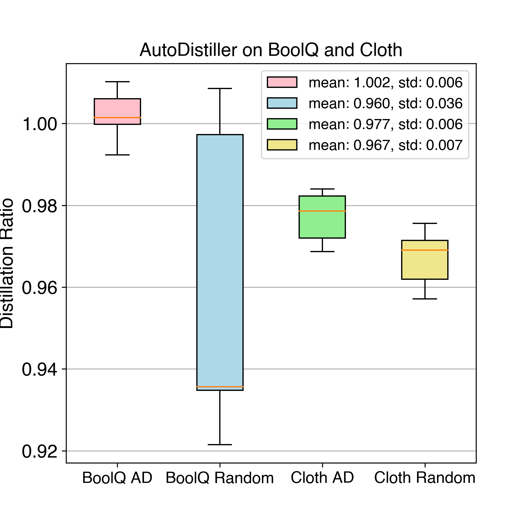
Figure 4: Distillation ratio of AutoDistiller (AD) top-5 KD strategies vs. 5 randomly selected strategies, for a fine-tuned $\text{BERT}_{\text{BASE}}$ teacher and $\text{TinyBERT}_{4}$ student. Higher ratio indicates better distillation performance. Mean and standard deviation of the four groups of ratios are listed in the legend.

6 Conclusion

We provided a systematic study of KD algorithms in NLP to understand the importance of different components in the KD pipeline for various NLP tasks. Using data collected from our study, we fit a AutoDistiller to predict student performance under each KD pipeline based on dataset features, which is helpful for automatically selecting which KD pipeline to use for a new dataset. Here we unified the existing intermediate distillation objectives as maximizing the lower bounds of MI, leading to a new MI-$\alpha$ objective based on tighter bounds, which performs better on many datasets.

Appendix –  Distiller: A Systematic Study of Model Distillation Methods
in Natural Language Processing

Appendix A Relationship with Other Distillation Methods

Distiller is a generic meta-framework that encompasses various KD pipelines used in previous work. For example, Distiller with the following configurations corresponds to the KD pipeline used in each of the cited works: $l^{\text{pred}}=$ CE, $l^{\text{inter}}=$ MSE, $m_{i,j}=$ Skip, $a=$ CA Jiao et al. (2020); $l^{\text{pred}}=$ CE, $l^{\text{inter}}=$ MSE, $m_{i,j}=$ EMD Li et al. (2020); $l^{\text{pred}}=$ CE, $a=$ Mixup Liang et al. (2021).

Appendix B Proof of Theorem 3.1

We denote the Mutual Information (MI) between two random variables $X$ and $Y$ as $I(X;Y)$. Based on the results on variational bounds of MI Poole et al. (2019), we derived that optimizing common knowledge distillation objectives, including Mean Squared Error (MSE), L2 distance, and cosine similarity between $X$ and $Y$, can be viewed as maximizing certain lower bounds of $I(X;Y)$.

Lemma B.1 ($I_{\text{TUBA}}$)

. Assume that $f(x,y)$ is an arbitrary neural network that takes $x$ and $y$ as inputs and outputs a scalar and $a(y)>0$. The lower bound of $x$ and $y$ can be estimated by:

$$I(X;Y) \geq E_{p(x,y)}[\log\frac{e^{f(x,y)}}{a(y)}]-E_{p(x)p(y)}[\frac{e^{f(x,y)}}{a(y)}]$$

$$\triangleq I_{\text{TUBA}}$$

Proof.

Based on the definition of MI, we have:

$$I(X;Y) =E_{p(x,y)}[\log\frac{p(x|y)}{p(x)}]$$ (5)

$$=E_{p(x,y)}[\log\frac{p(y|x)}{p(y)}]$$

Replacing the intractable conditional distribution $p(x|y)$ with a tractable variational distribution $q(x|y)$ yields a lower bound on MI due to the non-negativity of the KL divergence:

$$I(X;Y) =E_{p(x,y)}[\log\frac{q(x|y)}{p(x)}]+E_{p(x,y)}[\log\frac{p(x|y)}{q(x|y)}]$$

$$=E_{p(x,y)}[\log\frac{q(x|y)}{p(x)}]+E_{p(y)}[KL({p(x|y)}||{q(x|y)})]$$ (6)

$$\geq E_{p(x,y)}[\log q(x|y)]+H(X)$$

where $H(X)$ is the entropy of $X$.
We choose an energy-based variational family that uses a critic $f(x,y)$ and scaled by the data density $p(x)$:

$$q(x|y)=\frac{p(x)}{Z(y)}e^{f(x,y)},Z(y)=E_{p(x)}[e^{f(x,y)}]$$ (7)

Substituting this distribution into (B) gives a lower bound on MI:

$I(X;Y)\geq E_{p(x,y)}[f(x,y)]-E_{p(y)}[\log Z(y)]$

However, this objective is still intractable. To form a tractable bound, we can upper bound the log partition function by this inequality: $\log(x)\leq\frac{x}{a}+\log(a)-1$ for all $x,a>0$. Apply this inequality to get:

$$\begin{split}I(X;Y)&\geq E_{p(x,y)}[f(x,y)]-E_{p(y)}[\log Z(y)]\\ &\geq E_{p(x,y)}[f(x,y)]\\ &-E_{p(y)}[\frac{E_{p(x)}[e^{f(x,y)}]}{a(y)}+\log a(y)-1]\\ &=E_{p(x,y)}[f(x,y)]-E_{p(x,y)}[\log a(y)]\\ &-E_{p(x)p(y)}[\frac{e^{f(x,y)}}{a(y)}]+1\\ &\geq E_{p(x,y)}[\log\frac{e^{f(x,y)}}{a(y)}]-E_{p(x)p(y)}[\frac{e^{f(x,y)}}{a(y)}]\end{split}$$ (8)

This bound holds for any $a(y)>0$

Theorem 1.

Minimizing the MSE, L2, PKD loss, and maximizing the cosine similarity between two random variables $x$,$y$ can be viewed as maximizing lower bounds of $I(X;Y)$. In knowledge distillation, $x$ and $y$ are hidden states generated by student model and teacher model.

Proof. We prove this theorem by constructing $f(x,y)$ and $a(y)$ in Lemma B.1 for each loss function.

MSE

$L_{\text{MSE}}(x,y)=||x-y||_{2}^{2}$, let $f(x,y)=-||x-y||_{2}^{2},a(y)=1$, we have:

$$\begin{split}I(X;Y)&\geq E_{p(x,y)}[\log e^{-||x-y||_{2}^{2}}]-E_{p(x)p(y)}[e^{-||x-y||_{2}^{2}}]\\ &\geq E_{p(x,y)}[\log e^{-||x-y||_{2}^{2}}]-E_{p(x)p(y)}[e^{0}]\\ &=E_{p(x,y)}[\log e^{-||x-y||_{2}^{2}}]-1\\ &=E_{p(x,y)}[-||x-y||_{2}^{2}]-1.\end{split}$$

Thus, minimizing the MSE loss between $x$ and $y$ can be viewed as maximizing the lower bound of $I(X;Y)$.

PKD Loss

$L_{\text{PKD}}(x,y)=||\frac{x}{||x||_{2}}-\frac{y}{||y||_{2}}||_{2}^{2}$, let $f(x,y)=-||\frac{x}{||x||_{2}}-\frac{y}{||y||_{2}}||_{2}^{2}$, we have:

$$\begin{split}I(X;Y)&\geq E_{p(x,y)}[\log e^{-||\frac{x}{||x||_{2}}-\frac{y}{||y||_{2}}||_{2}^{2}}]\\ &-E_{p(x)p(y)}[e^{-||\frac{x}{||x||_{2}}-\frac{y}{||y||_{2}}||_{2}^{2}}]\\ &\geq E_{p(x,y)}[\log e^{-||\frac{x}{||x||_{2}}-\frac{y}{||y||_{2}}||_{2}^{2}}]-E_{p(x)p(y)}[e^{0}]\\ &=E_{p(x,y)}[\log e^{-||\frac{x}{||x||_{2}}-\frac{y}{||y||_{2}}||_{2}^{2}}]-1\\ &=E_{p(x,y)}[-||\frac{x}{||x||_{2}}-\frac{y}{||y||_{2}}||_{2}^{2}]-1.\end{split}$$ (9)

Thus, minimizing the PKD loss between $x$ and $y$ can be viewed as maximizing the lower bound of $I(X;Y)$.

L2 Loss

$L_{L_{2}}(x,y)=||x-y||_{2}$, let $f(x,y)=-||x-y||_{2}$, a(y)=1, we have:

$$\begin{split}I(X;Y)&\geq E_{p(x,y)}[\log e^{-||x-y||_{2}}]-E_{p(x)p(y)}[e^{-||x-y||_{2}}]\\ &\geq E_{p(x,y)}[\log e^{-||x-y||_{2}}]-E_{p(x)p(y)}[e^{0}]\\ &=E_{p(x,y)}[\log e^{-||x-y||_{2}}]-1\\ &=E_{p(x,y)}[-||x-y||_{2}]-1\end{split}$$

Thus, minimizing L2 loss between $x$ and $y$ is equivalent to maximizing the lower bound of $I(X,Y)$.

Cosine Similarity

The cosine similarity between two hidden states $x$ and $y$ is calculated as $\frac{x\cdot y}{||x||\times||y||}$, let $f(x,y)=\frac{x\cdot y}{||x||\times||y||}-1,a(y)=1$

$$\begin{split}I(X,Y)&\geq E_{p(x,y)}[\log e^{\frac{x\cdot y}{||x||\times||y||}-1}]-E_{p(x)p(y)}[e^{\frac{x\cdot y}{||x||\times||y||}-1}]\\ &\geq E_{p(x,y)}[\log e^{\frac{x\cdot y}{||x||\times||y||}-1}]-E_{p(x)p(y)}[e^{0}]\\ &=\frac{1}{e}E_{p(x,y)}[\log e^{\frac{x\cdot y}{||x||\times||y||}}]-1\\ &=\frac{1}{e}E_{p(x,y)}[\frac{x\cdot y}{||x||\times||y||}]-1\end{split}$$

Thus, maximizing cosine similarity between $x$ and $y$ can be viewed as maximizing mutual information between $x$ and $y$.

Table 4: Comparison of evaluation results on GLUE test set. We compare the distillation performance when using MLP and Transformer as critic functions in MI-$\alpha$ respectively. $\text{BERT}_{\text{BASE}}$ (T) indicates the teacher model trained by ourselves. Both of the students are initialized with $\text{TinyBERT}_{4}$ Jiao et al. (2020) and distilled with “Skip” as intermediate layer mapping strategy and MI-$\alpha$ as intermediate objective functions. The difference is, $\text{TinyBERT}_{4}$ (MLP) is trained with a 4-layer MLP with hidden state of 512 as critic function while $\text{TinyBERT}_{4}$ (Transformer) uses a 2-layer Transformer with feed-forward hidden size 256. The result shows that a small Transformer architecture performs as a better critic function than an MLP in MI-$\alpha$ especially when the task is a token-level task (SQuAD v1.1).

Model	MNLI-m	MNLI-mm	QQP	QNLI	SST-2	CoLA	MRPC	RTE	STS-B	SQuAD v1.1	AVG
	(393k)	(393k)	(364k)	(108k)	(67k)	(8.5k)	(3.5k)	(2.5k)	(5.7k)	(108k)
$\text{BERT}_{\text{BASE}}$ (T)	84.5	83.6	71.7	90.9	93.4	49.3	87.0	67.3	84.7	88.2	80.0
$\text{TinyBERT}_{4}$ (MLP)	81.7	80.6	69.7	87.6	91.6	24.9	87.0	67.4	81.9	70.1	74.3
$\text{TinyBERT}_{4}$ (Transformer)	81.9	80.6	69.8	87.4	91.5	25.9	87.0	67.4	84.0	71.7	74.7

Table 5: Comparison of evaluation results on GLUE dev set. We compare the distillation performance with(out) intermediate distillation. A $\text{BERT}_{\text{BASE}}$ model is used as the teacher and $\text{TinyBERT}_{4}$ is the student. $\text{TinyBERT}_{4}$ (KD) represents using a vanilla knowledge distillation (student only learns from the outputs of teacher) and “+intermediate distillation” represents using vanilla KD and intermediate distillation.

Model	MNLI-m	MNLI-mm	QQP	QNLI	SST-2	CoLA	MRPC	RTE	STS-B	SQuAD v1.1	AVG
	(393k)	(393k)	(364k)	(108k)	(67k)	(8.5k)	(3.5k)	(2.5k)	(5.7k)	(108k)
	acc	acc	f1/acc	acc	acc	mcc	f1/acc	acc	spearman/pearson	f1/em
$\text{BERT}_{\text{BASE}}$ (T)	84.1	84.7	88.0/91.1	91.7	93.0	55.0	89.6/85.0	65.0	88.4/88.6	88.2/80.9	83.8
$\text{TinyBERT}_{4}$ (KD)	80.1	80.3	86.4/89.7	85.8	89.1	16.1	89.6/85.3	66.8	88.4/88.5	77.3/66.8	77.9
+intermediate distillation	80.7	81.3	87.0/90.2	86.8	90.0	21.3	89.3/84.8	65.3	88.2/88.4	79.4/69.4	78.7

Appendix C Architecture of Teacher and Student Networks

In Table 1, we use two baseline models $\text{BERT-PKD}_{4}$ and $\text{BERT-EMD}_{4}$. As described in the original paper Sun et al. (2019), we initialize $\text{BERT-PKD}_{4}$ with the first 4 layers of parameters from pretrained $\text{BERT}_{\text{BASE}}$. $\text{BERT-EMD}_{4}$ is initialized from $\text{TinyBERT}_{4}$ so they have the same architecture. We list the detailed configurations of the teacher and student architectures investigated in our study in Table 6.

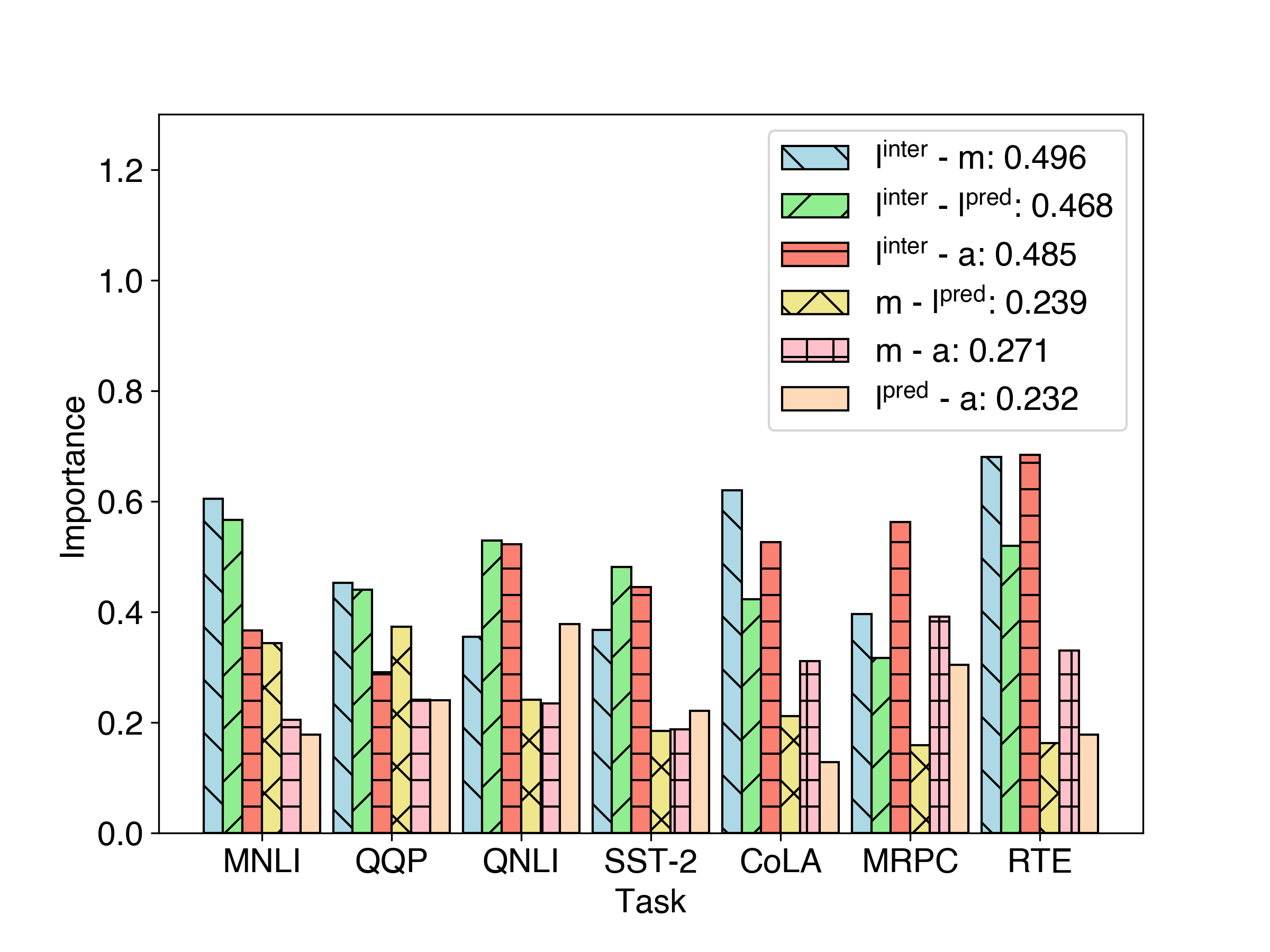
Figure 6: Importance of interactions between hyper-parameters.

Table 6: Network architectures of the teacher and student models used in the paper.

Model	#Params	$h_{\text{units}}$	$n_{\text{layers}}$	$h_{\text{mid}}$	$n_{\text{heads}}$
Teacher architectures
$\text{RoBERTa}_{\text{LARGE}}$	335M	1024	24	4096	16
$\text{ELECTRA}_{\text{LARGE}}$	335M	1024	24	4096	16
$\text{BERT}_{\text{BASE}}$	110M	768	12	3072	12
Student architectures
$\text{TinyBERT}_{\text{6}}$	67M	768	6	3072	12
$\text{BERT-PKD}_{4}$	52M	768	4	3072	12
$\text{BERT}_{\text{MEDIUM}}$	41M	512	8	2048	8
$\text{BERT}_{\text{SMALL}}$	29M	512	4	2048	8
$\text{TinyBERT}_{\text{4}}$	14M	312	4	1200	12
$\text{ELECTRA}_{\text{SMALL}}$	14M	256	12	1024	4
$\text{BERT}_{\text{MINI}}$	11M	256	4	1024	4
$\text{BERT}_{\text{TINY}}$	4M	128	2	512	2

Appendix D Benefits of Intermediate Distillation

Table 5 shows the experimental results of distillation with(out) intermediate distillation across different tasks/datasets. All the experiments are trained 20 epochs and the intermediate distillation constitutes of “Skip” as intermediate mapping strategy and CE as intermediate distillation object.

Appendix E Dataset Embedding

As features for the AutoDistiller model, we extract features from datasets and represent them as a fixed dimension embedding. Details are shown in Table 7.

Table 7: We extract features from downstream datasets so that every task can be represented as a fixed-dimension embedding. The extracted embedding can be fed into AutoDistiller as dense features. In this table, we describe how the embedding is acquired.

Feature	Description
Context Embedding	Every document can be represented as a weighted average of the GloVe vectors, where the weights are defined by the TF-IDF scheme. Each down-stream dataset is viewed as a “document” in the TF-IDF scheme. Precisely, the embedding of a dataset $s$ is $v_{s}=\frac{1}{|s|}\text{IDF}_{w}v_{w}$, where $|s|$ denotes the number of words in the dataset, and $\text{IDF}_{w}:=\log\frac{1+N}{1+N_{w}}$ is the inverse document frequency of word $w$. $N$ is the total number of datasets, and $N_{w}$ denotes the number of datasets containing $w$. Intuitively, this feature represents the content of datasets.
Task Embedding	For the dataset, we collect their literal descriptions, usually one or two sentences. Then aggregate GloVe vectors of every words in these sentences and get a description embedding. This feature is used to represent what is the NLP task and how the data is formatted.
Baseline Score	We use a lite Bi-LSTM model as the baseline model and finetune it on the down-stream dataset. This feature aims to measure the difficulty of each task by measuring how well a simple architecture can perform on the specific dataset.
Teacher Score	The fine-tuned teacher score on the dataset. Comparing teacher score to aforementioned baseline score tells how much boost can a complex model has on this dataset.
Number of Examples	How many training samples in the dataset.

Appendix F How much does larger/better teacher help?

Table 8 shows the performance of different students distilled from teachers of different sizes and pretraining schemes. From the results, we found that although the teacher $\text{ELECTRA}_{\text{LARGE}}$ has the best performance on average score, most of the students of $\text{ELECTRA}_{\text{LARGE}}$ performs worse than students of $\text{RoBERTa}_{\text{LARGE}}$. $\text{ELECTRA}_{\text{SMALL}}$ is the only student that performs the best with $\text{ELECTRA}_{\text{LARGE}}$ as teacher, that may be attributed to $\text{ELECTRA}_{\text{SMALL}}$ and $\text{ELECTRA}_{\text{LARGE}}$ are pretrained on the same pretraining task, so they have a similar knowledge representation scheme. And also, for datasets (MNLI, QQP, QNLI and SST-2) which have abundant amount of data, students of $\text{BERT}_{\text{BASE}}$ perform better.

Table 8: Performance comparison with different teacher and student models. We abbreviate three teacher models $\text{BERT}_{\text{BASE}}$,$~{}\text{RoBERTa}_{\text{LARGE}}$ and $\text{ELECTRA}_{\text{LARGE}}$ as B, R, E. Results are evaluated on GLUE dev set and best results are in-bold.

Model	#Params	Teacher	MNLI-m	MNLI-mm	QQP		QNLI	SST-2	CoLA	MRPC		RTE	STS-B		AVG
			acc	acc	f1	acc	acc	acc	mcc	f1	acc	acc	spearman	pearson
$\text{BERT}_{\text{BASE}}~{}\text{(T)}$	110M		84.1	84.7	88.0	91.1	91.7	93.0	55.0	89.6	85.0	65.0	88.4	88.6	83.7
$\text{RoBERTa}_{\text{LARGE}}~{}\text{(T)}$	335M		90.2	90.1	89.6	92.1	94.7	96.3	64.6	91.3	88.0	78.7	91.7	91.8	88.3
$\text{ELECTRA}_{\text{LARGE}}~{}\text{(T)}$	335M		90.5	90.4	90.3	92.8	95.1	96.6	67.4	91.7	88.5	84.5	88.7	88.9	88.8
$\text{BERT}_{\text{BASE}}$	110M	R	84.5	84.6	88.6	91.5	91.7	93.2	59.3	91.6	88.0	66.4	89.0	89.4	84.8
		E	84.4	84.6	88.8	91.7	91.6	92.8	59.5	91.9	88.7	69.3	89.1	89.6	85.2
$\text{TinyBERT}_{\text{6}}$	67M	B	83.9	84.0	88.1	91.2	91.3	91.6	50.5	90.3	86.5	75.5	89.4	89.4	84.3
		R	83.5	83.5	88.0	91.2	90.8	92.2	48.0	91.9	88.7	72.6	89.9	90.0	84.2
		E	83.0	83.0	87.8	91.0	90.6	91.3	48.6	91.6	88.5	76.2	89.1	89.3	84.2
$\text{BERT}_{\text{MEDIUM}}$	41M	B	82.6	83.0	87.9	91.0	90.0	90.8	48.3	88.9	84.1	65.0	88.2	88.4	82.4
		R	80.9	81.4	87.6	90.8	89.0	91.4	50.5	88.9	84.6	64.3	88.2	88.6	82.2
		E	81.0	81.3	87.5	90.7	89.0	90.9	51.0	89.5	85.3	64.3	88.0	88.2	82.2
$\text{BERT}_{\text{SMALL}}$	29M	B	81.0	81.0	87.4	90.6	87.3	90.5	43.1	87.8	82.4	63.5	87.0	87.2	80.7
		R	78.7	78.6	87.0	90.4	87.0	88.6	41.2	89.1	84.1	64.3	87.1	87.3	80.3
		E	78.6	78.8	87.2	90.5	87.0	89.3	43.0	88.7	84.1	63.9	86.8	87.1	80.4
$\text{TinyBERT}_{\text{4}}$	14M	B	81.1	81.6	87.2	90.4	87.4	90.6	12.3	89.4	85.0	66.4	87.7	87.8	78.9
		R	80.0	80.7	86.5	90.0	86.0	89.4	24.6	90.4	86.5	67.9	88.0	88.1	79.8
		E	80.0	80.2	86.2	89.6	85.9	88.9	21.8	90.9	86.8	68.6	87.6	87.6	79.5
$\text{ELECTRA}_{\text{SMALL}}$	14M	B	82.7	83.8	87.8	90.9	89.7	91.3	60.6	91.3	87.7	60.6	87.4	87.5	83.5
		R	82.3	83.2	88.1	91.2	89.5	90.6	58.6	91.3	87.5	67.5	87.6	87.8	83.8
		E	82.0	82.7	88.5	91.5	89.3	91.4	60.6	92.3	89.0	69.7	86.6	86.7	84.2
$\text{BERT}_{\text{MINI}}$	11M	B	78.5	79.7	86.6	90.0	84.9	87.8	20.1	87.0	81.6	61.0	86.2	86.1	77.5
		R	76.6	77.3	86.0	90.0	84.6	85.9	32.2	86.6	81.1	65.3	86.2	86.3	78.2
		E	76.3	77.1	85.9	89.5	84.2	85.9	33.8	87.0	81.6	65.0	85.7	85.5	78.1
$\text{BERT}_{\text{TINY}}$	4M	B	72.8	73.4	83.5	87.2	81.3	83.9	0.0	84.5	75.7	58.5	81.4	79.9	71.8
		R	71.5	72.0	82.9	86.7	80.2	83.1	6.2	84.9	76.2	60.3	81.9	79.9	72.1
		E	71.2	71.8	82.9	87.0	80.0	82.8	6.7	85.2	77.0	62.8	78.4	77.3	71.9

Appendix G Computing Details

All the experiments are performed on a single machine with 4 NVIDIA T4 GPUs. For hyper-parameters in Equation 1, our experiments suggest that setting $\beta_{1}$ and $\beta_{2}$ to $1$ produces the best overall performance so we fix their values to $1$ in subsequent results. $\gamma_{1}$ and $\gamma_{2}$ are set to $0.5$ when DA is used (otherwise $\beta_{2}$, $\gamma_{1}$ and $\gamma_{2}$ are set to $0$). For controlled experiments, unless specified explicitly, we fix ${l^{\text{inter}}}$ as MI-$\alpha$ $(\alpha=0.9)$ and the layer mapping as “Skip”. Critic functions in MI-$\alpha$ are powered by a two-layer Transformer($h_{\text{mid}}=256$, $n_{\text{heads}}=8$) and the comparison of using Transformer and MLP to estimate critic functions is described in Table 4. To reduce the hyper-parameter search space, we fix the batch size as 16 and the learning rate as 5e-5 for all experiments. We used automated mix precision for training. Maximum sequence length is set to 128 for sentence-pair tasks in GLUE, 64 for single sentence tasks and 320 for SQuAD. Most of the experiments are trained for 20 epochs except 50 epochs for the challenging task CoLA and 30 epochs for SQuAD.

Appendix H Distiller Search Space

Here we recap the full search space considered for each stage of the KD pipeline in Distiller:

• $l^{\text{inter}}$ $\in$ {MSE, L2, Cos, PKD, MI-$\alpha$ ($\alpha$ = 0.1, 0.5, or 0.9)}

• $l^{\text{pred}}$ $\in$ {MSE, CE}

• {$m_{i,j}$} $\in$ {Skip, Last, EMD}

• Augmentation policy $a$ is one or combinations of elementary augmentation operations in {CA, RA, BT, Mixup}.

Appendix I Top Configurations in Distiller

Here we list the top 5 configurations from the Distiller search space that performed best on each dataset in Table 9.

Table 9: Top 5 configurations to distill a $\text{BERT}_{\text{BASE}}$ teacher to a $\text{TinyBERT}_{4}$ student on every dataset. To reduce the search space, we only compare configurations that don’t use data augmentation. As Hyper-parameter $\alpha$ is only valid for MI-$\alpha$, the value of $\alpha$ is set to N for other intermediate loss in the table.

Task	Intermediate Loss	$\alpha$	Layer Mapping Strategy	KD Loss	#Example	Score
MNLI	MI-$\alpha$	0.9	EMD	MSE	393000	81.7
MNLI	MI-$\alpha$	0.1	EMD	MSE	393000	81.7
MNLI	MI-$\alpha$	0.5	Skip	MSE	393000	81.7
MNLI	MSE	N	EMD	MSE	393000	81.6
MNLI	MSE	N	Skip	MSE	393000	81.6
QQP	MI-$\alpha$	0.9	EMD	MSE	364000	90.2
QQP	MI-$\alpha$	0.1	EMD	MSE	364000	90.2
QQP	CE	N	Skip	MSE	364000	90.2
QQP	MI-$\alpha$	0.1	EMD	MSE	364000	90.1
QQP	MI-$\alpha$	0.1	Skip	MSE	364000	90.1
QNLI	CE	N	Last	MSE	105000	87.4
QNLI	MI-$\alpha$	0.5	Skip	MSE	105000	87.4
QNLI	MI-$\alpha$	0.5	Last	CE	105000	87.3
QNLI	MI-$\alpha$	0.9	Skip	CE	105000	87.2
QNLI	MI-$\alpha$	0.1	Skip	CE	105000	87.1
SST-2	Cos	N	Last	MSE	67000	90.6
SST-2	MSE	N	Skip	CE	67000	90.5
SST-2	MI-$\alpha$	0.1	Last	CE	67000	90.3
SST-2	CE	N	Skip	MSE	67000	90.3
SST-2	MI-$\alpha$	0.9	Skip	CE	67000	90.3
CoLA	MI-$\alpha$	0.1	EMD	MSE	8500	22.3
CoLA	MI-$\alpha$	0.5	EMD	MSE	8500	21.6
CoLA	MI-$\alpha$	0.5	EMD	CE	8500	21.1
CoLA	MI-$\alpha$	0.1	Last	MSE	8500	21.1
CoLA	MI-$\alpha$	0.5	Skip	MSE	8500	21.0
MRPC	MI-$\alpha$	0.1	EMD	CE	3700	90.3
MRPC	MI-$\alpha$	0.5	EMD	CE	3700	90.2
MRPC	CE	N	Skip	CE	3700	89.9
MRPC	MI-$\alpha$	0.9	EMD	CE	3700	89.9
MRPC	CE	N	Last	MSE	3700	89.7
RTE	MI-$\alpha$	0.1	Skip	CE	2500	70.8
RTE	MI-$\alpha$	0.9	Skip	CE	2500	70.4
RTE	MI-$\alpha$	0.5	Skip	CE	2500	70.0
RTE	MI-$\alpha$	0.1	Last	CE	2500	70.0
RTE	MI-$\alpha$	0.5	Last	CE	2500	69.3
STS-B	MI-$\alpha$	0.9	Skip	MSE	7000	88.0
STS-B	MI-$\alpha$	0.5	Skip	MSE	7000	88.0
STS-B	MI-$\alpha$	0.9	EMD	MSE	7000	87.9
STS-B	MI-$\alpha$	0.1	Last	MSE	7000	87.9
STS-B	PKD	N	Skip	MSE	7000	87.9
SQuAD v1.1	MSE	N	Skip	MSE	130000	72.6
SQuAD v1.1	CE	N	Skip	MSE	130000	72.4
SQuAD v1.1	MSE	N	EMD	MSE	130000	72.3
SQuAD v1.1	MI-$\alpha$	0.9	Skip	CE	130000	71.9
SQuAD v1.1	MI-$\alpha$	0.9	Skip	CE	130000	71.7

References

- Blei et al. (2017) David M Blei, Alp Kucukelbir, and Jon D McAuliffe. 2017. Variational inference: A review for statisticians. Journal of the American Statistical Association, 112(518):859–877.
- Brown et al. (2020) Tom Brown, Benjamin Mann, Nick Ryder, Melanie Subbiah, Jared D Kaplan, Prafulla Dhariwal, Arvind Neelakantan, Pranav Shyam, Girish Sastry, Amanda Askell, Sandhini Agarwal, Ariel Herbert-Voss, Gretchen Krueger, Tom Henighan, Rewon Child, Aditya Ramesh, Daniel Ziegler, Jeffrey Wu, Clemens Winter, Chris Hesse, Mark Chen, Eric Sigler, Mateusz Litwin, Scott Gray, Benjamin Chess, Jack Clark, Christopher Berner, Sam McCandlish, Alec Radford, Ilya Sutskever, and Dario Amodei. 2020. Language models are few-shot learners. In Advances in Neural Information Processing Systems.
- Buciluǎ et al. (2006) Cristian Buciluǎ, Rich Caruana, and Alexandru Niculescu-Mizil. 2006. Model compression. In Proceedings of the 12th ACM SIGKDD international conference on Knowledge discovery and data mining, pages 535–541.
- Chen et al. (2020) Daoyuan Chen, Yaliang Li, Minghui Qiu, Zhen Wang, Bofang Li, Bolin Ding, Hongbo Deng, Jun Huang, Wei Lin, and Jingren Zhou. 2020. Adabert: Task-adaptive bert compression with differentiable neural architecture search. In IJCAI.
- Clark et al. (2020) Kevin Clark, Minh-Thang Luong, Quoc V Le, and Christopher D Manning. 2020. ELECTRA: Pre-training text encoders as discriminators rather than generators. In ICLR.
- Cubuk et al. (2019) Ekin D Cubuk, Barret Zoph, Dandelion Mane, Vijay Vasudevan, and Quoc V Le. 2019. AutoAugment: Learning augmentation strategies from data. In CVPR, pages 113–123.
- Devlin et al. (2019) Jacob Devlin, Ming-Wei Chang, Kenton Lee, and Kristina Toutanova. 2019. BERT: Pre-training of deep bidirectional transformers for language understanding. In NAACL.
- Donsker and Varadhan (1975) Monroe D Donsker and SR Srinivasa Varadhan. 1975. Asymptotic evaluation of certain markov process expectations for large time, i. Communications on Pure and Applied Mathematics, 28(1):1–47.
- Edunov et al. (2018) Sergey Edunov, Myle Ott, Michael Auli, and David Grangier. 2018. Understanding back-translation at scale. arXiv preprint arXiv:1808.09381.
- Erickson et al. (2020) Nick Erickson, Jonas Mueller, Alexander Shirkov, Hang Zhang, Pedro Larroy, Mu Li, and Alexander Smola. 2020. Autogluon-tabular: Robust and accurate automl for structured data. arXiv preprint arXiv:2003.06505.
- Fakoor et al. (2020) Rasool Fakoor, Jonas W Mueller, Nick Erickson, Pratik Chaudhari, and Alexander J Smola. 2020. Fast, accurate, and simple models for tabular data via augmented distillation. In Advances in Neural Information Processing Systems, volume 33.
- Guo et al. (2019) Hongyu Guo, Yongyi Mao, and Richong Zhang. 2019. Augmenting data with mixup for sentence classification: An empirical study. arXiv preprint arXiv:1905.08941.
- Gupta and Agrawal (2020) Manish Gupta and Puneet Agrawal. 2020. Compression of deep learning models for text: A survey. arXiv preprint arXiv:2008.05221.
- Hinton et al. (2014) Geoffrey Hinton, Oriol Vinyals, and Jeff Dean. 2014. Distilling the knowledge in a neural network. In NIPS 2014 Deep Learning Workshop.
- Hou et al. (2020) Lu Hou, Zhiqi Huang, Lifeng Shang, Xin Jiang, Xiao Chen, and Qun Liu. 2020. DynaBERT: Dynamic bert with adaptive width and depth. In Advances in Neural Information Processing Systems.
- Hutter et al. (2014) Frank Hutter, Holger Hoos, and Kevin Leyton-Brown. 2014. An efficient approach for assessing hyperparameter importance. In ICML, pages 754–762. PMLR.
- Jiao et al. (2020) Xiaoqi Jiao, Yichun Yin, Lifeng Shang, Xin Jiang, Xiao Chen, Linlin Li, Fang Wang, and Qun Liu. 2020. TinyBERT: Distilling BERT for natural language understanding. In EMNLP.
- Kaplan et al. (2020) Jared Kaplan, Sam McCandlish, Tom Henighan, Tom B Brown, Benjamin Chess, Rewon Child, Scott Gray, Alec Radford, Jeffrey Wu, and Dario Amodei. 2020. Scaling laws for neural language models. arXiv preprint arXiv:2001.08361.
- Kim et al. (2021) Taehyeon Kim, Jaehoon Oh, NakYil Kim, Sangwook Cho, and Se-Young Yun. 2021. Comparing kullback-leibler divergence and mean squared error loss in knowledge distillation. In IJCAI.
- Kong et al. (2020) Lingpeng Kong, Cyprien de Masson d’Autume, Wang Ling, Lei Yu, Zihang Dai, and Dani Yogatama. 2020. A mutual information maximization perspective of language representation learning. In ICLR.
- Li et al. (2020) Jianquan Li, Xiaokang Liu, Honghong Zhao, Ruifeng Xu, Min Yang, and Yaohong Jin. 2020. BERT-EMD: Many-to-many layer mapping for bert compression with earth mover’s distance. In EMNLP.
- Liang et al. (2021) Kevin J Liang, Weituo Hao, Dinghan Shen, Yufan Zhou, Weizhu Chen, Changyou Chen, and Lawrence Carin. 2021. MixKD: Towards efficient distillation of large-scale language models. In ICLR.
- Liu et al. (2019) Yinhan Liu, Myle Ott, Naman Goyal, Jingfei Du, Mandar Joshi, Danqi Chen, Omer Levy, Mike Lewis, Luke Zettlemoyer, and Veselin Stoyanov. 2019. RoBERTa: A robustly optimized bert pretraining approach. arXiv preprint arXiv:1907.11692.
- Mirzadeh et al. (2020) Seyed Iman Mirzadeh, Mehrdad Farajtabar, Ang Li, Nir Levine, Akihiro Matsukawa, and Hassan Ghasemzadeh. 2020. Improved knowledge distillation via teacher assistant. In AAAI.
- Nguyen et al. (2010) XuanLong Nguyen, Martin J Wainwright, and Michael I Jordan. 2010. Estimating divergence functionals and the likelihood ratio by convex risk minimization. IEEE Transactions on Information Theory, 56(11):5847–5861.
- Oord et al. (2018) Aaron van den Oord, Yazhe Li, and Oriol Vinyals. 2018. Representation learning with contrastive predictive coding. arXiv preprint arXiv:1807.03748.
- Pennington et al. (2014) Jeffrey Pennington, Richard Socher, and Christopher D. Manning. 2014. Glove: Global vectors for word representation. In EMNLP, pages 1532–1543.
- Poole et al. (2019) Ben Poole, Sherjil Ozair, Aaron Van Den Oord, Alex Alemi, and George Tucker. 2019. On variational bounds of mutual information. In ICML.
- Raffel et al. (2019) Colin Raffel, Noam Shazeer, Adam Roberts, Katherine Lee, Sharan Narang, Michael Matena, Yanqi Zhou, Wei Li, and Peter J Liu. 2019. Exploring the limits of transfer learning with a unified text-to-text transformer. arXiv preprint arXiv:1910.10683.
- Rajpurkar et al. (2016) Pranav Rajpurkar, Jian Zhang, Konstantin Lopyrev, and Percy Liang. 2016. SQuAD: 100,000+ questions for machine comprehension of text. In EMNLP.
- Sanh et al. (2019) Victor Sanh, Lysandre Debut, Julien Chaumond, and Thomas Wolf. 2019. DistilBERT, a distilled version of BERT: smaller, faster, cheaper and lighter. arXiv preprint arXiv:1910.01108.
- Shi et al. (2021) Xingjian Shi, Jonas Mueller, Nick Erickson, Mu Li, and Alex Smola. 2021. Multimodal automl on structured tables with text fields. In 8th ICML Workshop on Automated Machine Learning (AutoML).
- Sun et al. (2019) Siqi Sun, Yu Cheng, Zhe Gan, and Jingjing Liu. 2019. Patient knowledge distillation for BERT model compression. In EMNLP.
- Tschannen et al. (2020) Michael Tschannen, Josip Djolonga, Paul K Rubenstein, Sylvain Gelly, and Mario Lucic. 2020. On mutual information maximization for representation learning. ICLR.
- Turc et al. (2019) Iulia Turc, Ming-Wei Chang, Kenton Lee, and Kristina Toutanova. 2019. Well-read students learn better: On the importance of pre-training compact models. arXiv preprint arXiv:1908.08962.
- Vaswani et al. (2017) Ashish Vaswani, Noam Shazeer, Niki Parmar, Jakob Uszkoreit, Llion Jones, Aidan N Gomez, Łukasz Kaiser, and Illia Polosukhin. 2017. Attention is all you need. In Advances in neural information processing systems, pages 5998–6008.
- Wang et al. (2019a) Alex Wang, Yada Pruksachatkun, Nikita Nangia, Amanpreet Singh, Julian Michael, Felix Hill, Omer Levy, and Samuel R Bowman. 2019a. Superglue: A stickier benchmark for general-purpose language understanding systems. arXiv preprint arXiv:1905.00537.
- Wang et al. (2019b) Alex Wang, Amanpreet Singh, Julian Michael, Felix Hill, Omer Levy, and Samuel R Bowman. 2019b. GLUE: A multi-task benchmark and analysis platform for natural language understanding. In ICLR.
- Wei and Zou (2019) Jason Wei and Kai Zou. 2019. EDA: Easy data augmentation techniques for boosting performance on text classification tasks. In EMNLP.
- Yang et al. (2021) Jing Yang, Brais Martinez, Adrian Bulat, and Georgios Tzimiropoulos. 2021. Knowledge distillation via softmax regression representation learning. In ICLR.
- Zhang et al. (2018) Hongyi Zhang, Moustapha Cisse, Yann N Dauphin, and David Lopez-Paz. 2018. Mixup: Beyond empirical risk minimization. In ICLR.