IE-GAN: An Improved Evolutionary Generative Adversarial Network Using a New Fitness Function and a Generic Crossover Operator
Abstract
The training of generative adversarial networks (GANs) is usually vulnerable to mode collapse and vanishing gradients. The evolutionary generative adversarial network (E-GAN) attempts to alleviate these issues by optimizing the learning strategy with multiple loss functions. It uses a learning-based evolutionary framework, which develops new mutation operators specifically for general deep neural networks. However, the evaluation mechanism in the fitness function of E-GAN cannot truly reflect the adaptability of individuals to their environment, leading to an inaccurate assessment of the diversity of individuals. Moreover, the evolution step of E-GAN only contains mutation operators without considering the crossover operator jointly, isolating the superior characteristics among individuals. To address these issues, we propose an improved E-GAN framework called IE-GAN, which introduces a new fitness function and a generic crossover operator. In particular, the proposed fitness function, from an objective perspective, can model the evolutionary process of individuals more accurately. The crossover operator, which has been commonly adopted in evolutionary algorithms, can enable offspring to imitate the superior gene expression of their parents through knowledge distillation. Experiments on various datasets demonstrate the effectiveness of our proposed IE-GAN in terms of the quality of the generated samples and time efficiency.
Index Terms:
Deep generative models, evolutionary strategy, generative adversarial networks, knowledge distillation.I Introduction
Generative adversarial networks (GANs) [1], as deep learning models, have been widely used in synthesis tasks [2, 3]. The losses of GANs can be exploited by adaptation learning methods to bridge the gap between cross-domain distributions [4]. However, the training of GANs is notoriously difficult, as it commonly encounters several problems, such as mode collapse and vanishing gradients [5]. To address these issues, evolutionary computation has been introduced to stabilize the training processes of GANs. Specifically, evolutionary computation techniques are utilized to perform the selection of generators [6], discriminators [7], or even input noise [8] by using multiple individuals, which form a population in the selection process. A single individual encoded as a genotype can represent a neural network in an abstract way. Actually, there exist many different types of encoded genes, such as network structures and weights. A genotype is often bijectively mapped to the phenotype of an individual. The choice of individuals is based on the evaluation of the phenotype, with the goal of producing a better solution in the next generation of the population. In this research, we refer to the combination of GANs and evolutionary computation as evolutionary GANs.
The evolutionary generative adversarial network (E-GAN) [6] is a typical evolutionary GAN, that maintains a generator population to generate individuals with different loss functions, which are referred to as mutation operators. In each evolution step in E-GAN, individuals are evaluated in terms of their quality and diversity. Due to the success of E-GAN, many researchers have tried to further improve the performance of E-GAN. For example, the cooperative dual evolution-based GAN (CDE-GAN) [7] expands the concept of a population to the discriminator and uses a soft mechanism to connect two populations that compete with each other during the evolution process. Moreover, Mu et al. [9] defined a novel mutation operator, i.e., a distribution indicating realness, to replace the original mutation operator in E-GAN. At the same time, the multi-objective evolutionary GAN (MO-EGAN) [10] and smart MO-EGAN (SMO-EGAN) [11] consider quality and diversity as conflicting objectives, and they model the evaluation of generators as a multi-objective problem. In addition, mutation spatial GANs (Mustangs) [12] applies different loss functions to a competitive co-evolutionary algorithm. In addition to the E-GAN-based methods, there are many other studies on evolutionary GANs [13, 14, 15, 8, 16]. Nevertheless, each of these methods usually has weaknesses with respect to the individual evaluation process or the crossover operator.
An evolutionary strategy requires an appropriate fitness function to assess the adaptability of individuals to their environment. The fitness function models the researcher’s expectation of the evolutionary trend of a population and is an essential guarantee of the effectiveness of an evolutionary strategy. Specifically, for the generative model, a fitness function evaluates the samples generated by individuals. Nevertheless, determining how to measure the diversity of the generated samples is also a controversial problem. The Fréchet inception distance (FID) [17], which can reflect samples’ diversity, is often utilized as a typical metric for generative performance during testing. The resource requirements of the FID, however, make it unsuitable for use in the training phase of methods with a large number of iterations. As a result, E-GAN uses a discriminator-based diversity metric. However, according to our observations from experiments, we found that this metric cannot be as effective as expected for E-GAN.
On the other hand, there are two common but crucial variation operators in evolutionary computation, i.e., mutation and crossover. The mutation operator produces new characteristics, while the crossover operator is used to combine the best characteristics of multiple individuals. Currently, evolutionary GANs rarely consider the crossover operator. Although Garciarena et al. applied the crossover operator in [16], their defined crossover operator is rather difficult to adapt to other methods. In [16], pairs of generators and discriminators regarded as evolving individuals are crossed by exchanging paired objects. The cross-variance implementation dictates that the operator is only applicable to methods that have pairwise generators and discriminators. Moreover, this crossover strategy can only expand the population diversity; it cannot make the offspring collect the superior characteristics of their parents, due to the fact that the neural network does not reflect gene dominance or recessiveness, which play an important role in biological inheritance.
In this research, we propose an improved E-GAN framework called IE-GAN to address these existing shortcomings of evolutionary GANs. Specifically, IE-GAN introduces an objective fitness function and a generic crossover operator to evolutionary GANs. Our proposed fitness function considers the perspective of individual phenotypes, which is more accurate while balancing the time cost; the diversity part of the fitness function is based on gene expression without relying on other training entities, and the quality part of the fitness function is adjusted accordingly. The -filtered knowledge distillation crossover in IE-GAN also starts from the phenotype rather than directly manipulating genes like -point crossover, a typical crossover operator for evolutionary computation. This learning-based crossover operator allows offspring to imitate the gene expression of their parents through knowledge distillation and preserve the learned knowledge in their genotypes, which protects the training stability of the GAN. In essence, IE-GAN directs the exploration direction of possible solutions in the parameter space more accurately with fewer resources while exploiting the valuable parts of multiple trials. Extensive experiments on multiple datasets show that our method has advantages over state-of-the-art methods in terms of both the generative performance and training time, and it can alleviate mode collapse and vanishing gradients; it is also quite robust.
To summarize, the main contributions of this paper are as follows:
-
•
We analyze and experimentally verify the imperfection of E-GAN. The fitness function of E-GAN has difficulty modeling the environmental pressure on the population, and therefore, it cannot guide the population in the desired direction. E-GAN also lacks a crossover operator and forgets the valuable experience of individuals who did not survive.
-
•
We propose a concise but efficient fitness function that can accurately reflect the individuals’ adaptation to the environment. Unlike previous functions, it can objectively measure the variance of the generated samples while requiring less time.
-
•
We introduce a generic learning-based crossover operator that clusters the superior characteristics of multiple networks irrespective of specific network implementations. To the best of our knowledge, this is the first crossover operator that is widely applicable to methods that consider deep networks as individuals.
-
•
We design and implement a framework called IE-GAN with our crossover operator and fitness function. Experiments show that our method has significant advantages in terms of the training stability, generative performance, and training time. This framework is also robust and can be easily applied to other evolutionary GANs.
II Related Work
II-A E-GAN
E-GAN [6] uses an adversarial framework with a discriminator and a population of generators to improve the stability and generative capability of GANs. Specifically, it assumes that the generators no longer exist as individuals; instead, they are a population that competes with the discriminator. From an evolutionary point of view, the discriminator can be considered a changing environment during the evolutionary process.
In each evolution step of E-GAN, the evolution of the generator consists of three steps: variation, evaluation, and selection. The variation includes only the mutation operation, and different loss functions are chosen as mutation operators to produce different offspring. Then, the generative performance of the generated offspring needs to be evaluated and quantified using the corresponding fitness value. We will call the fitness function in [6] in this paper to avoid confusion. After measuring the generative performance of all offspring, according to the principle of survival of the fittest, the updated generators are selected as the parents for a new round of training.
The mutation operator used by E-GAN is more suitable for deep neural networks than random mutations that imitate organisms. A framework based on gradient learning rather than randomness allows the population to remain small and allows the system to converge to meaningful results relatively quickly. This evolutionary strategy guided by loss functions is more conducive to system stability. Meanwhile, this evolutionary process derived from learning is easily extended to other algorithms and tasks. In view of the above advantages of E-GAN, Li et al. created an E-GAN with crossover (CE-GAN) in [18], which is a preliminary step for this work.
II-B Knowledge Distillation
Knowledge distillation is a model compression method and training method based on the teacher-student network in which the knowledge contained in a trained model is distilled and applied to the target model [19]. The target model is often a smaller model that is compressed and has better generalizability. The target model can learn to match any layer of the trained model, including intermediate feature maps of different sizes [20]. Hard targets learn from the output, which reduces the training time but increases the possibility of overfitting. Soft targets learn from logits, which contain more descriptive information about the samples and enable the target network to have better generalization capabilities [19].
As a means of compressing networks, knowledge distillation has been applied to GANs [21, 22]. Proximal distilled evolutionary reinforcement learning (PDERL) [23] utilizes this technique to optimize evolutionary reinforcement learning (ERL) [24]. It utilized a learning-based crossover operator called the -filtered behavior distillation crossover operator. Experiments demonstrate that in reinforcement learning (RL), this operator can ensure that offspring inherit the behaviors of their parents. Thus, -filtered behavior distillation crossover will not cause destructive interference like -point crossover. Moreover, -filtered behavior distillation crossover as a learning-based variation can be easily accelerated using graphics processing units (GPUs), and it is useful even for deeper networks. The crossover operator proposed in this paper is also implemented based on knowledge distillation.
II-C Gradient Penalty
The gradient penalty (GP) [25] achieves the Lipschitz constraint required by the Wasserstein GAN (WGAN) [26]. It replaces the weight clipping of WGAN and effectively avoids the concentration of weights on the clipping threshold, so the network will not push weights towards two values. Additionally, because it eliminates the setting of the clipping threshold, the network will not suffer from vanishing or exploding gradients because of an unreasonable threshold setting. The application space of the GP has been extended from the image space to separable Banach spaces [27].
III Preliminaries
III-A Notation
We refer to the symbols used in [29, 6]. GANs can generally be formulated as follows:
| (1) |
| (2) |
where , , , and are scalar-to-scalar functions, and the GAN and its variants with different loss functions use different versions of these functions. is the distribution of real data, and is the distribution of the sampling noise (usually a uniform or normal distribution). is the generative network without the final activation layer, and is an activation layer, which is in the deep convolutional GAN (DCGAN) [30]. , where is the output of the generator and its distribution is expected to be fitted to . is the discriminative network without the final activation layer. In most GANs, can be interpreted as indicating how realistic the input data are [29]. In the original GAN [1], , where is the output of the discriminative network .
III-B Fitness Function
An evaluation criterion to measure the quality of individuals is needed in the evolutionary algorithm. Existing methods utilize various fitness functions, such as the inverted generational distance (IGD) [16], Koncept512 [8], and its variants [6, 7, 9, 10], and a mixture of GAN objective functions and the FID [12, 14].
The fitness function [6] is written as follows:
| (3) |
where balances two measurements. The output of the discriminator w.r.t. the generated samples is used as the quality fitness :
| (4) |
The diversity fitness function is formally expressed as
| (5) |
The diversity fitness is the negative log-gradient-norm of the loss function of . The logarithm is used to shrink the fluctuation of the gradient norm, which differs from the output of the discriminator by an order of magnitude, and the amplitude is so large that a simple balance coefficient cannot balance the two values.
E-GAN assumes that the more discrete the generated samples are, the less likely the discriminator is to change the parameters substantially. embodies this principle. However, our experiments show that not only cannot achieve this design purpose but also causes obvious negative side effects.
IV Method
This section describes the details of our proposed IE-GAN, especially the main contributions of the evaluation of individuals and crossover.
IV-A IE-GAN Framework
The IE-GAN framework designed in this paper evolves a population of generators in a given dynamic environment (discriminator ) and a static environment (diversity fitness function), where is the size of the population. Each individual in the population represents a possible solution in the parameter space [6]. The IE-GAN framework is shown in Fig. 1.
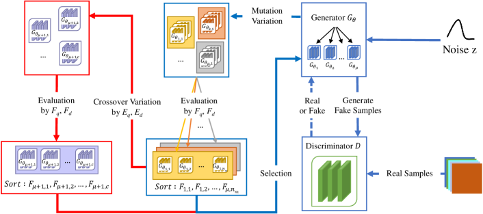
In each evolution step, individuals in the population act as parents to generate offspring using mutation operators, where is the number of mutation operators. After evaluating mutation individuals using the fitness function , their environmental fitness is obtained. Then crossover parents are selected according to these fitness scores, and crossover individuals are obtained using the crossover operator, where is the number of crossover individuals. Next, the fitness of crossover individuals is evaluated. Finally, the offspring with high fitness scores are selected as the parents of the next generation.
After the evolution step, the discriminator is updated. Thus the dynamic environment also changes with the evolution of the population, and it is able to provide continuous evolutionary pressure in conjunction with the static environment. The objective function of is the same as that of the original GAN [1], except for the additional GP term [25], i.e.,
| (6) |
where the third subterm is a GP term. is the intermediate distribution between the real data and generated data. is the balance coefficient of the GP, which is set to as in WGAN-GP [25].
The IE-GAN framework implemented in this paper adopts the same three mutation operators as E-GAN: the minimax (in GAN [1]), heuristic (in NS-GAN [5]), and least-squares (in LSGAN [31]) operators. The complete algorithm is similar to the framework algorithm in [18]. In comparison to the two-player game of traditional GANs, E-GAN makes it possible to select different dominant adversarial targets in different training phases. Furthermore, CE-GAN [18] can integrate the advantages of multiple loss functions in each training phase to generate advantageous individuals. Moreover, IE-GAN improves the crossover operator of CE-GAN and is able to guide evolution with a more accurate evaluation function, thereby obtaining a more competitive solution. It is worth mentioning that the discriminator is deeply involved in the entire framework. It provides gradient information for mutation operators, and it provides an important measurement that is used to evaluate samples and offspring. Therefore, the framework can strongly benefit from the improvement of .
IV-B Mutation
The evaluation function and the crossover operator of IE-GAN, both of which act on the generated samples, are independent of the network implementation. Therefore, the IE-GAN framework is independent of the genes encoded. It has no hard and fast rules for the mutation operators, as long as the mutation operators can proliferate the parents into several different mutation individuals. As a result, the IE-GAN framework, which does not introduce additional constraints, can be easily applied to existing evolutionary GANs with generators as individuals.
IV-C Evaluation
The FID is a common generation task metric in the literature [32, 33, 34, 35, 36, 37]; it reflects both the quality and diversity of the samples. It can also be used as a fitness function to guide evolution in an evolutionary strategy. However, its higher time complexity makes it suitable only for methods with fewer evolutionary generations; otherwise the excessive time cost will make the method useless.
calculates the environmental fitness score of an individual by evaluating the samples it generates. It splits the assessment metric into two aspects: the quality fitness score and the diversity fitness score. However, equation (5) cannot fully express the diversity fitness score. In fact, is affected not only by diversity but also by quality. As an example, if the generated sample distribution hardly overlaps with the true sample distribution, can almost accurately distinguish the two types of samples. When the network hardly changes the parameters, the evaluation object will become unduly competitive. To put it simply, low-quality samples will receive high diversity fitness scores. This is the problem: not only fails to reflect diversity but also hinders the quality evaluation of , which makes the training vulnerable to the vanishing gradients problem when the balance coefficient is not appropriate. Furthermore, the nonlinear scaling of amplifies its negative effects, and even the most careful adjustment of the balance coefficients can easily cause the evaluation results to be dominated by a single submetric. In addition, requires additional computation for the gradient information of the discriminator, which increases the time cost significantly.
Rather than relying on synchronous training discriminators like , we expect the diversity fitness function to measure individuals objectively. Instead of indirectly evaluating the diversity of the generators using a discriminator, we directly evaluate the distributional distance of the samples produced by the generators. Therefore, we propose a new diversity fitness function, which estimates the diversity in terms of the mean absolute error (MAE) between samples. The generative diversity of individuals is measured by the sample dissimilarity. Formally, our diversity fitness function is defined as follows:
| (7) |
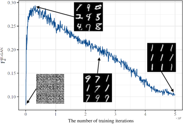
where refers to the number of times each sample is compared with other samples. It is the mean w.r.t. the MAE of each sample. The fitness function is easy to compute, which is helpful to algorithms that require a large number of iterations. The function is also robust and insensitive to outliers, which keeps the global perspective from being overly influenced by local differences. Moreover, the MAE of a single sample can also be considered as the evaluation of the sample itself, which helps the subsequent crossover operator to make full use of the evaluated samples. As shown in Fig. 2, experiments on the MNIST111http://yann.lecun.com/exdb/mnist/ dataset demonstrate that our fitness function can objectively reflect the sample diversity.
Additionally, our quality fitness function also differs from equation (4) by replacing in with . The Sigmoid layer does not change the sorting but affects the output values. When combined with the diversity component, the presence or absence of the Sigmoid layer may lead to changes in the fitness sorting. Given that can represent the truthfulness of the data [29], we believe that is a more suitable function to use to assess the quality fitness. The formal definition of our quality fitness function is as follows:
| (8) |
Its essence is the evaluation of the sample quality using the discriminator. It can measure a single sample without additional operations, and therefore it can be used to filter samples in the crossover operation.
By combining the above two fitness functions, the fitness function of the IE-GAN framework can be obtained:
| (9) |
where balances the two metrics. A higher value indicates that the evaluated object has a better generative performance.
IV-D Crossover
In this subsection, we present the -filtered knowledge distillation crossover operator w.r.t. the -filtered behavior distillation crossover operator [23]. Due to the difference between GANs and RL, our crossover operator differs from this previous crossover operator in some aspects, including sample filtering and basic network. Fig. 3 illustrates the flow of a crossover operation.
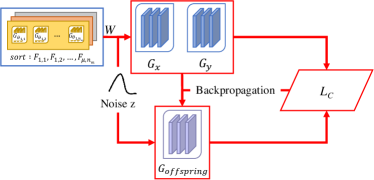
The crossover operation of a pair of parent networks is as follows:
-
•
The model with a higher fitness score among the parents is used as the basis of the offspring model, and the results generated by the parents with the same inputs are used as experiences for the offspring to learn from.
-
•
The knowledge of the parents is transferred to the offspring through knowledge distillation.
Note that the parents mentioned in the definition of the crossover operation are the mutation individuals generated by the mutation operators rather than the original parents of each generation.
The outputs of parents for the same inputs are likely to be completely different. Thus, a natural question is the following: how can the offspring imitate both networks at the same time? The solution is that the offspring choose the better output to imitate for each input. The definition of whether a sample is good or bad is left to . The higher the value, the more worthy of study a given output is. is defined as follows:
| (10) |
where is a parameter used to balance the two metrics. This evaluation also considers both the quality and diversity of samples:
| (11) |
| (12) |
where is a sample from the same batch as .
The formal representation of the -filtered knowledge distillation loss used to train the offspring is as follows:
| (13) |
where and represent the generative strategies of the parents. and are the inactive outputs of their corresponding generators, and represents an inactive output of the offspring. We believe that fitting with soft targets helps the offspring inherit more information. The offspring network learns the knowledge of the parents by minimizing the function during training. The whole procedure of the crossover operator is similar to the -filtered knowledge distillation crossover algorithm in [18]. It requires the hyperparameter crossover batch size, which is denoted by .
There is still a problem: how should the algorithm select parents from among the multiple networks for crossover? We use the greedy strategy score function defined in [23]:
| (14) |
This strategy usually results in the selection of better individuals, which ensures the excellence of the resulting offspring and increases the stability of the population [23]. Since crossover parents and the initial network of crossover offspring need to be selected based on individual evaluation, it is necessary to evaluate mutation individuals before crossover. Given that the assessments of both individuals and samples are considered in terms of the quality and diversity, the samples generated and the fitness scores obtained in the evaluation substage can be reused in the crossover substage.
This operator can act on the phenotype space [22] or the extracted intermediate features [21]. Knowledge distillation is independent of the topological differences between the teacher network and student network, but if learning from feature extraction is taking place, it is a challenge to select matches from the constantly changing network architecture for an evolutionary strategy that encodes the topology as genes. In view of this, we choose to perform imitation learning from the end of network so that this method can be applied to a more general framework.
The crossover operator proposed in this paper is somewhat different from crossover variation in the biological sense. In biology, the phenotypic characteristics of offspring are determined by gene expression, and the dominance of inherited characteristics is reflected by the dominance of genes (usually the characteristics represented by dominant genes are better). In short, gene crossover determines the inheritance of characteristics. The basis for realising our crossover operator is learning the expression of superior parental characteristics in the phenotype space and inscribing the knowledge in the network weights. The superior characteristics are judged by the offspring themselves. The entire process does not require the participation of genes. Because of this gene-independence, the -filtered knowledge distillation crossover operator does not care about the genes encoded by the individuals of the population.
IV-E Selection
There are two issues related to the selection of the next generation of parents: whether or not the mutation individuals are still candidates, and whether or not the current parents are candidates. For the former issue, we have experimentally demonstrated that only using crossover offspring will not bring significant gains, and doing so does not reduce the computational complexity. Therefore, mutation offspring should not be excluded from selection. As for the latter issue, existing studies use updated discriminators to re-evaluate current parents and treat them as parent candidates for the next generation [7, 10]. Experiments on our framework show that this strategy enhances the training stability. However, it will slow down convergence, negatively affect the final result, and increase the computational effort. Therefore, we do not consider transferring the current parents to the next generation.
V Experiments
To verify the effectiveness of the IE-GAN framework, we conducted extensive experiments with its algorithmic implementation on several generative tasks, and we present the results in this section. The experiments show that IE-GAN can achieve a competitive performance with high efficiency. In addition, we analyze some details of the method.
V-A Experimental Configuration
We conduct experiments on two synthetic datasets and two real-world image datasets, CIFAR-10 [38] and CelebA [39]. The two synthetic datasets are a 2D mixture of eight Gaussians arranged in a circle and a 2D mixture of 25 Gaussians arranged in a grid. Because the distributions of the generated data and target data can be visualized, such toy datasets are often used to demonstrate the mode collapse of a method. CIFAR-10 is a dataset for identifying universal objects that contains ten categories of RGB color images of objects in the real world. The images in this dataset are noisy, and the proportions and features of the objects are also different, which makes recognition difficult. The size of the images is . CelebA is a large-scale face attribute dataset with a large number of celebrity images. The images in this dataset have pose variations and background clutter.
For comparison purposes, the generator and discriminator networks for CIFAR-10 are the same as those in E-GAN [6]; they are fine-tuned DCGAN networks [30]. As for CelebA, we adopt the official PyTorch implementation222https://github.com/pytorch/examples/tree/master/dcgan of the DCGAN architecture. To cope with the complex dataset CelebA, we apply more channels in the convolutional layers and transposed convolutional layers. In addition, we choose the multilayer perceptron (MLP) as the model architecture for the toy experiments. The target distribution of the synthetic data and the corresponding network architectures in the experiments are taken from the third-party PyTorch implementation333https://github.com/caogang/wgan-gp of WGAN-GP. The model architecture applied in this paper is shown in detail in Table I. In addition to the network architectures, the GP settings of the two types of datasets are also different. In order to better reflect the performance differences of each method on synthetic datasets, experiments on the eight Gaussians and 25 Gaussians do not use the GP term.
| Generative Network | Discriminative Network |
| E-GAN | |
| Input: Noise , 100 | Input: Image () |
| layer 1 Transposed Convolution (4, 4, 512), stride=1; ReLU; | layer 1 Convolution (4, 4, 128), stride=2; LeakyReLU; |
| layer 2 Transposed Convolution (4, 4, 256), stride=2; ReLU; | layer 2 Convolution (4, 4, 256), stride=2; Batchnorm; LeakyReLU; |
| layer 3 Transposed Convolution (4, 4, 128), stride=2; ReLU; | layer 3 Convolution (4, 4, 512), stride=2; Batchnorm; LeakyReLU; |
| layer 4 Transposed Convolution (4, 4, 3), stride=2; Tanh; | layer 4 Fully Connected (1); Sigmoid; |
| Output: Generated Image () | Output: Real or Fake (Probability) |
| DCGAN | |
| Input: Noise , 100 | Input: Image () |
| layer 1 Transposed Convolution (4, 4, 1024), stride=1; Batchnorm; ReLU; | layer 1 Convolution (4, 4, 128), stride=2; LeakyReLU; |
| layer 2 Transposed Convolution (4, 4, 512), stride=2; Batchnorm; ReLU; | layer 2 Convolution (4, 4, 256), stride=2; Batchnorm; LeakyReLU; |
| layer 3 Transposed Convolution (4, 4, 256), stride=2; Batchnorm; ReLU; | layer 3 Convolution (4, 4, 512), stride=2; Batchnorm; LeakyReLU; |
| layer 4 Transposed Convolution (4, 4, 128), stride=2; Batchnorm; ReLU; | layer 4 Convolution (4, 4, 1024), stride=2; Batchnorm; LeakyReLU; |
| layer 5 Transposed Convolution (4, 4, 3), stride=2; Tanh; | layer 5 Convolution (4, 4, 1), stride=1; Sigmoid; |
| Output: Generated Image () | Output: Real or Fake (Probability) |
| MLP | |
| Input: Noise , 2 | Input: Point () |
| layer 1 Fully Connected (512); ReLU; | layer 1 Fully Connected (512); ReLU; |
| layer 2 Fully Connected (512); ReLU; | layer 2 Fully Connected (512); ReLU; |
| layer 3 Fully Connected (512); ReLU; | layer 3 Fully Connected (512); ReLU; |
| layer 4 Fully Connected (2); | layer 4 Fully Connected (1); Sigmoid; |
| Output: Generated Point () | Output: Real or Fake (Probability) |
The values of the hyperparameters shared with E-GAN have the same values that they have in E-GAN. Specifically, the Adam optimizer with a learning rate , , and is used; the number of updating steps of the discriminator per iteration ; the number of mutations ; the mutation batch size ; and the sample size for evaluation . Additionally, we recommend a population size . However, the balance coefficient for the fitness quality and diversity (i.e., ) is an exception. This is due to how we redefine the quality and diversity fitness function. We select for the synthetic datasets and for the real-world datasets via grid search. For IE-GAN-specific hyperparameters, we choose , , and crossover size for all experiments. We set the crossover batch size to 256; it is equal to . In this paper, we conduct experiments with these values if not otherwise stated.
We use the FID [17] to quantitatively evaluate the generative performance. In fact, the FID is a metric that is widely used in a variety of image synthesis tasks, such as image generation [32, 33, 34] and image-to-image translation [35, 36, 37]. The FID is frequently used as a metric in studies concerning GANs, and it is considered superior to other metrics [40]. The lower the FID, the better the quality of the generated images. We randomly generate 50K images to calculate the FID during the test phase. Unless otherwise stated, the experiments in this paper are trained for 100K generations.
The experiments are conducted on a single NVIDIA TITAN Xp GPU with 12GB of memory and an Intel Xeon E5-2620 v2 CPU. The code we implemented in PyTorch is publicly available at https://github.com/AlephZr/IE-GAN.
V-B Mode Collapse
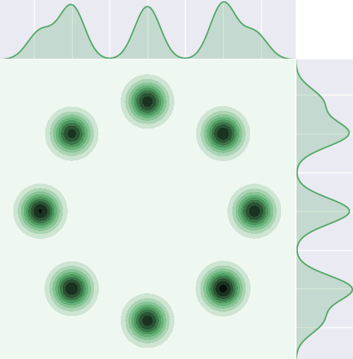
Learning the 2D Gaussian mixture distributions can visually demonstrate the mode collapse of the model. If the model suffers from mode collapse, the samples it generates will focus on a limited number of modes. This can be directly observed using kernel density estimation (KDE) plots.
We compare the complete algorithm of IE-GAN with the baselines, including GAN, NS-GAN, LSGAN, and E-GAN. For fairness, all methods utilize the same MLP network architecture. Because of the huge difference between synthetic and real-world datasets, the learning rate and the number of discriminator updates in each iteration are consistent with the source of the network architecture, i.e., and .
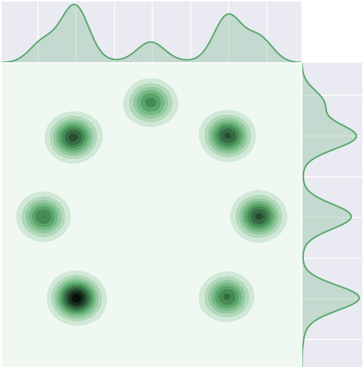
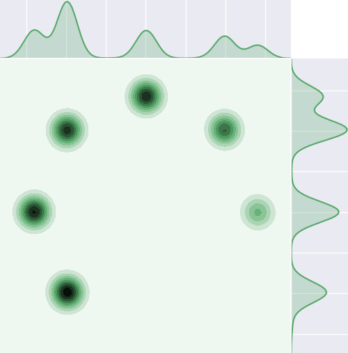
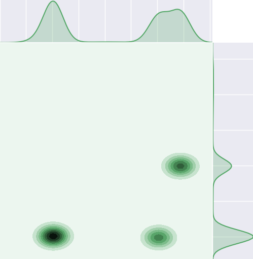
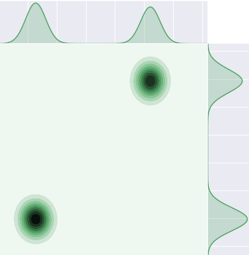
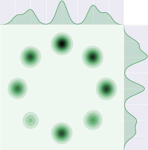
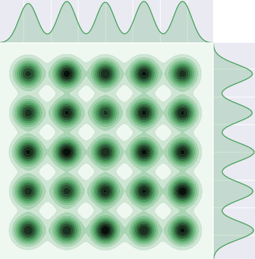
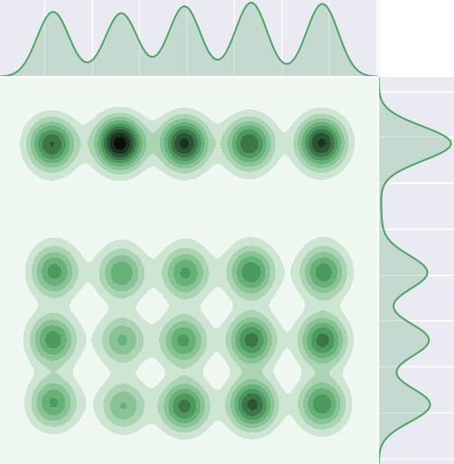
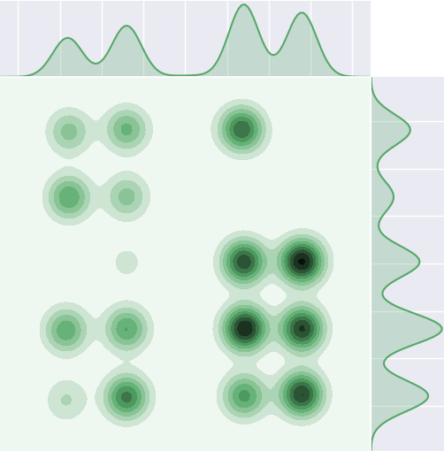
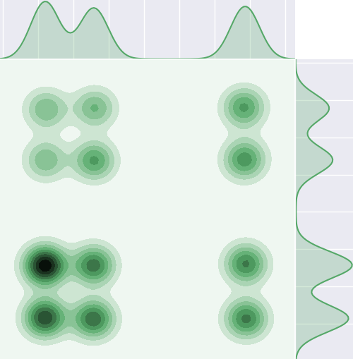
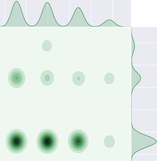
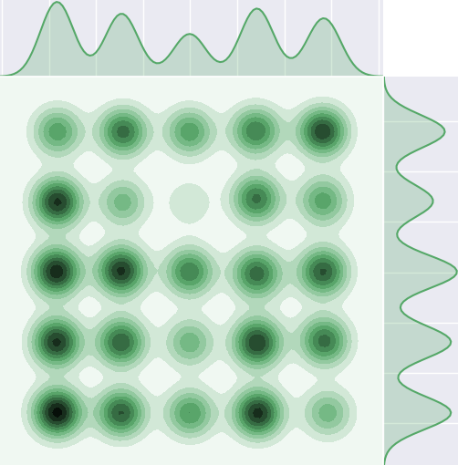
Fig. 4 illustrates the modes captured by different methods. The center plot of each plot is the KDE plot, and the side plots reflect the probability distribution. To adequately represent the generated distribution, 10,240 points are sampled for each plot. We can see that on both synthetic datasets, the baselines show some missing modes. This is especially true for E-GAN, which appears to be inapplicable to experimental networks. It performs the worst out of all the methods, and its evolutionary strategy exacerbates mode collapse. In contrast, IE-GAN is able to cover all modes (although some modes are weakly covered), which indicates that our evolutionary strategy can effectively suppress mode collapse. This is corroborated by the side plots, which show that the probability distribution of IE-GAN is closest to that of the target data.
| Target | GAN | NS-GAN | LSGAN | E-GAN | IE-GAN | |
|
8 Gaussians |
 |
 |
 |
 |
 |
 |
|
25 Gaussians |
 |
 |
 |
 |
 |
 |
V-C Generative Performance
To illustrate the superiority of the proposed IE-GAN over the baselines, we conduct experiments on the CIFAR-10 dataset [38]. The baselines used for comparison include GAN-Minimax, GAN-Heuristic, and GAN-Least-squares, which, respectively, represent the methods that use a single mutation operator. The experimental results obtained by comparing IE-GAN with these baselines are used to demonstrate that our approach benefits primarily from the framework rather than the network architecture. In order to explore the role of each operator, their settings are identical to those of IE-GAN, including , the discriminator objective function, and the GP. In addition, we compare IE-GAN with E-GAN [6] to demonstrate the effectiveness of the proposed evolutionary strategy. E-GAN likewise maintains only one population unless otherwise stated.
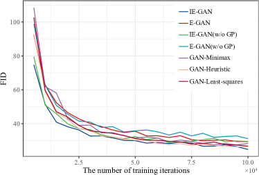
Fig. 5 plots the FID for the training process of different methods for the same network architecture. We use an experimental setup from the literature [6], along with codes444https://github.com/WANG-Chaoyue/EvolutionaryGAN-pytorch provided by previous authors, to obtain the results of E-GAN. The following conclusions can be drawn from this figure:
-
•
IE-GAN shows a more significant improvement in the generative performance than E-GAN due to the GP term. This is because the GP term acts on the discriminator, which is more deeply involved in IE-GAN. In addition to participating in normal gradient learning and in the evaluation, as in E-GAN, the discriminator in IE-GAN also takes part in the assessment of the samples during the crossover process. Therefore, IE-GAN can benefit more from discriminator enhancement.
-
•
The GP term also accelerates the convergence of IE-GAN, whereas E-GAN experiences no such acceleration. This is the work of the crossover operator. The discriminator is involved in crossover variation, so a better discriminator makes it possible to obtain better crossover offspring, which in turn accelerates the model convergence.
-
•
The crossover operator itself also contributes to the model convergence. IE-GAN without the GP shows a considerable convergence speed, and it is clearly distinguished from methods other than IE-GAN with the GP until 25K iterations.
-
•
IE-GAN does benefit from multiple operators, and it has the best generative performance and the fastest convergence speed. Most of the time, the fold line representing IE-GAN is at the bottom of the plot.
-
•
The evolutionary strategy of E-GAN works the other way around. Under the same conditions, E-GAN is worse than any of the single-mutation-operator methods. Its generative performance is only similar to that of IE-GAN without the GP term.
For comparison and analysis, the FID values of different methods including various populations of E-GAN are listed in Table II, where the data marked with are quoted from [6]. “Final FID” in the table denotes the FID after 100K iterations. The best value is bolded. We reproduced the multipopulation experiments of E-GAN, but perhaps because of the different experimental environments, the final results are different from those in [6]. The results of our experiment show the following:
-
•
The generative performance of E-GAN can be improved by increasing the population, but this improvement is insignificant. As the population size increases from one to eight, the FID decreases by less than one, and the number of maintained generative networks increases from 3 to 24, which increases the cost.
-
•
This improvement of E-GAN is also unstable. When , the experimental results are worse than they are for .
-
•
E-GAN does not benefit from multiple operators. The population brings such a small improvement that the performance at is likely to be close to the limit that E-GAN can achieve. Even so, E-GAN is still inferior to GAN-Minimax, which is the worst single-mutation-operator method. The results show that, due to the unreasonable evaluation function, E-GAN performs worse than any other reference baseline.
| Method | Final FID |
| GAN-Minimax | |
| GAN-Heuristic | |
| GAN-Least-squares | |
| E-GAN (, w/o GP) | |
| E-GAN () | |
| E-GAN () | |
| E-GAN () | |
| E-GAN () | |
| E-GAN (, w/o GP) | |
| E-GAN () | |
| E-GAN () | |
| E-GAN () | |
| E-GAN () | |
| IE-GAN (Ours) (, w/o GP) | |
| IE-GAN (Ours) () | 24.82 |
Finally, IE-GAN is compared with seven typical evolutionary GANs to demonstrate the advantages of its evolutionary strategies. The FIDs of all methods for the CIFAR-10 dataset are reported in Table III. “30K FID” in the table denotes the FID after 30K iterations to show the convergence speeds of the methods. Evolution-GAN [16], COEGAN [14], and QD-COEGAN [15] do not record 30K FIDs because of the differences in their training strategies. The best results are underlined. and in Table III represent the generator and discriminator population sizes maintained by the evolutionary methods, respectively. The experimental code for each method is obtained from the corresponding study, and the configuration refers to the source description.
| Method | 30K FID | Final FID |
| E-GAN () [6] | ||
| MO-EGAN () [10] | ||
| SMO-EGAN () [11] | ||
| CDE-GAN () [7] | ||
| Evolution-GAN () [16] | ||
| COEGAN () [14] | ||
| QD-COEGAN () [15] | ||
| IE-GAN (Ours) () | 12 | |
| CDE-GAN (IE-GAN framework) () | 24.33 |
-
1
The best results for the unmodified methods are underlined.
-
2
The best results out of all methods are shown in bold.
The experiments show that IE-GAN outperforms all baselines. The first group in Table III, the learning-based evolutionary GANs, all perform poorly compared to our IE-GAN. It is worth noting that the default numbers of iterations of MO-EGAN [10], SMO-EGAN [11] and CDE-GAN [7] are larger than the 100K iterations used by IE-GAN; MO-EGAN and SMO-EGAN run for 100 epochs (about 150K iterations), and CDE-GAN runs for 150K iterations. The second group of methods in Table III randomly vary the coding genes. Experiments demonstrate that an inherently unstable system like a GAN should not introduce excessive randomness when dealing with complex tasks. The disorderly direction of variation forces the population to maintain a large size, which results in greater resource use. Additionally, this disorderly exploration is too inefficient for complex task spaces to be competitive. In particular, Evolution-GAN [16], which has the strongest randomness among all methods and has a network structure that only supports fully connected layers, cannot achieve meaningful results on the CIFAR-10 dataset. Meanwhile, the framework of IE-GAN is applied to CDE-GAN to verify its generalizability. The experimental results are recorded in Table III. The best results are shown in bold. It can be seen that IE-GAN effectively improves the convergence speed and generation performance of CDE-GAN. Moreover, none of the hyperparameters involved in the experiments are tuned. This proves that IE-GAN has good robustness; it did not achieve good results because of carefully tuned hyperparameters.
V-D Time Cost
The runtime is also an important criterion for evaluating method usability. Fig. 6 shows the wall-clock time required to train different methods for 100K iterations on the CIFAR-10 dataset, and the length of each bar reflects the time cost of the corresponding method.
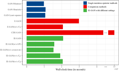
GAN-Minimax, GAN-Heuristic, and GAN-Least-squares maintain only one generator network and no additional evaluation of the generators is required, so the time cost of training these networks is similar and less than that of IE-GAN. Among the evolutionary GANs, the proposed IE-GAN shows a significant advantage in terms of the time cost. IE-GAN maintains four generative networks, while requiring about twice as much time as the single-mutation-operator methods. The time cost of E-GAN is obviously higher than that of IE-GAN, although it does not produce crossover offspring. While CDE-GAN maintains only three more networks than IE-GAN, its time cost is more than six times that of IE-GAN.
On the one hand, the dominance of IE-GAN is attributed to the relatively simple diversity fitness function. The IE-GAN experiments with different settings in Fig. 6 demonstrate the low consumption of . The reduction in the wall-clock time caused by removing from IE-GAN is very small. The calculation time of is the lowest out of all the components, and it has little effect on the time cost. In contrast, requires considerable calculations using the discriminator gradient information. As shown in Fig. 6, removing can effectively accelerate the training of E-GAN. On the other hand, the wall-clock time advantage of IE-GAN benefits from the streamlined framework structure. The reuse of the samples generated in the evaluation phase during crossover offspring learning minimizes the time needed by the training process. CDE-GAN requires more time due to the coevolution of the two populations. CDE-GAN maintains about twice the number of networks as E-GAN, but the wall-clock time is more than four times that of E-GAN. This suggests that it is inefficient not only because it inherits from E-GAN but also due to its competitive strategy. The two populations of CDE-GAN must score each other, which greatly increases the cost of evaluation. In summary, the efficient and the brief training process together result in the low time cost of IE-GAN.
V-E Ablation Study
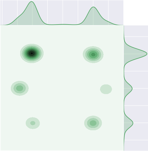
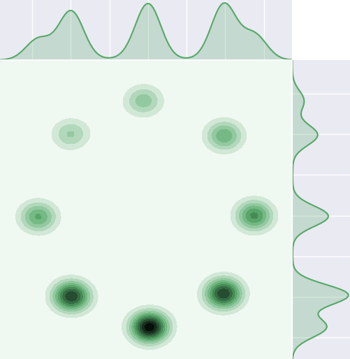
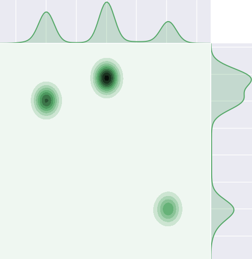
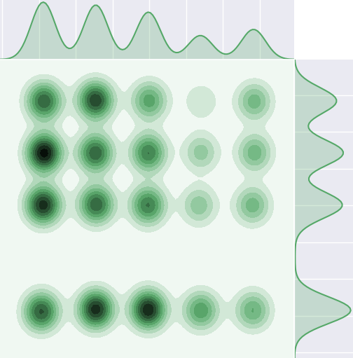
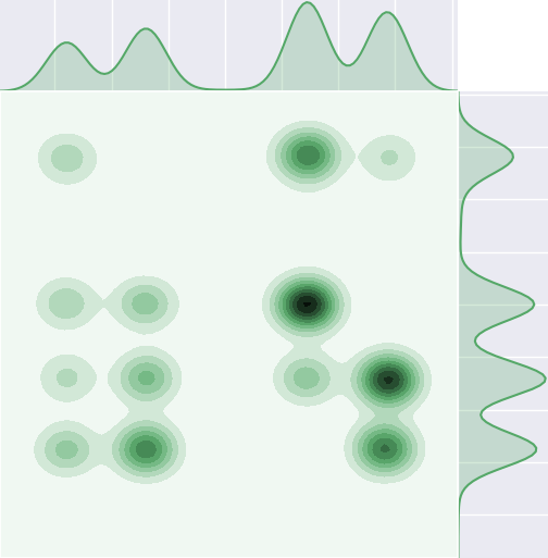
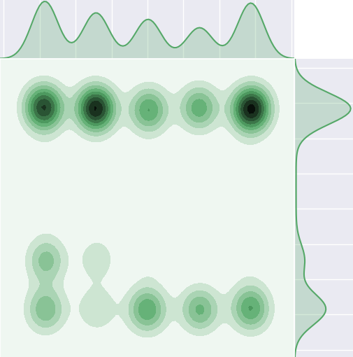
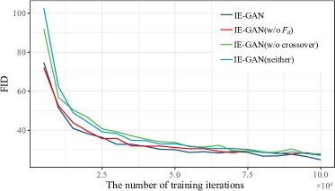
We compare IE-GAN with its ablation variants. Fig. 7 shows examples of IE-GAN and its ablation on the synthetic datasets. Eliminating or the crossover variation decreases the performance, and eliminating both leads to more serious consequences. This means that both and crossover support generative diversity. A similar conclusion can be obtained on the CIFAR-10 dataset. Fig. 8 shows that both items are critical to our method. In addition, the crossover operator exhibits its acceleration effect.
| Target | IE-GAN (w/o ) | IE-GAN (w/o crossover) | IE-GAN (neither) | IE-GAN | |
|
8 Gaussians |
 |
 |
 |
 |
 |
|
25 Gaussians |
 |
 |
 |
 |
 |
V-F Hyperparameter Analysis
We use the same discriminator objective function as E-GAN. There are two more hyperparameters that are closely related to the performance of IE-GAN, namely the balance coefficients of the fitness function () and the sample evaluation function (). Since they are used to balance quality and diversity measurements, they guide the selection of generators and samples, which affects the performance of IE-GAN. Meanwhile, the targets of the knowledge distillation of the crossover operator, the number of parents imitated by crossover offspring, the crossover batch size , and the number of sample comparisons all affect the effectiveness of IE-GAN. In this subsection, we analyze their effects one by one through experiments on CIFAR-10.
V-F1 Correlation
The fitness function represents the pressure of the environment on individuals. The effects of the two types of metrics, quality and diversity, in the individual fitness measure are balanced by the coefficient . This coefficient directly affects the selection of the population by the environment and must therefore be chosen carefully.
In order to guarantee confidence, we choose a larger population to ensure that there are enough individuals for each evaluation. In this way, the effect of the balance coefficient can be amplified so that the performances of the generators are sufficiently differentiated. In this experiment, the population size is set to . To eliminate the interference of the crossover operator and related hyperparameters, the crossover operator is not enabled in this experiment. We perform a grid search to find an appropriate value of . Table IV lists the performance measurements of the trained generators; the balance coefficients are used in the experiment. When , is not enabled. “Best FID” in the table represents the best FID of the method during the training process. The best value for each item is bolded.
| Method | Final FID | Best FID |
| IE-GAN () | ||
| IE-GAN () | ||
| IE-GAN () | ||
| IE-GAN () | 27.15 | 26.74 |
| IE-GAN () | ||
| IE-GAN () | ||
| IE-GAN () |
Whether the final FID or the best FID is considered, these values generally decrease first and then increase as increases. The exception is , which provides a better score than any of the values outside . This suggests that an inappropriate additional term is more likely to be a source of interference. The results show that the performance is correlated with , which leads to poorer consequences if it is too large or too small. This phenomenon occurs in experiments with different population sizes. We select for real-world image datasets based on observations.
V-F2 Correlation
The balance coefficient of the sample evaluation function affects the competitiveness of the crossover offspring by controlling the learning objects. Appropriate learning objects mean that the crossover offspring can collect more of the superior characteristics of the parents rather than their defects. The crossover operator that depends on is expected to generate dominant offspring, while the fitness function that includes represents the desired evolutionary direction. Although the two behave similarly, they should not be roughly equal.
In addition to the sample evaluation function, the knowledge distillation targets also affect the position of the crossover offspring in the population. Although softer targets are preferred in knowledge distillation [19], as they minimizes the information loss, their effectiveness should be experimentally verified in different algorithmic settings. Likewise, the number of crossover parents can affect system outcomes through the generated offspring. In principle, our crossover operator allows the offspring to learn from a set of networks rather than a limited set of two parents. If the crossover offspring is precise enough to absorb the experience of its parents, it can learn more from more trained networks.
Since all three hyperparameters (, knowledge distillation targets, and the nubmer of crossover parents) are related to the crossover operator and are tightly correlated, they are considered together here. We perform a grid search for in a total of four contexts combined with different knowledge distillation targets and numbers of crossover parents. We set the size of the population and the crossover size in this experiment. The performance measurements are reported in Table V. The best result in each context is bolded and the best result out of all contexts is additionally underlined.
| Soft Targets | Hard Targets | |||||
| Two Parents | Method | Final FID | Best FID | Method | Final FID | Best FID |
| IE-GAN () | IE-GAN () | |||||
| IE-GAN () | IE-GAN () | |||||
| IE-GAN () | IE-GAN () | 25.63 | 25.63 | |||
| IE-GAN () | IE-GAN () | |||||
| IE-GAN () | IE-GAN () | |||||
| IE-GAN () | IE-GAN () | |||||
| All Parents | Method | Final FID | Best FID | Method | Final FID | Best FID |
| IE-GAN () | IE-GAN () | |||||
| IE-GAN () | IE-GAN () | 26.19 | ||||
| IE-GAN () | 25.81 | 25.81 | IE-GAN () | |||
| IE-GAN () | IE-GAN () | 25.94 | ||||
| IE-GAN () | IE-GAN () | |||||
| IE-GAN () | IE-GAN () | |||||
-
1
The best results in each context are shown in bold.
-
2
The best results out of all contexts are underlined.
Within each context, equation (12) is counterproductive when is inappropriate, and gradually takes on a positive effect as tends toward 0.001 in general. This is not true in the context of hard targets when all mutation offspring are used as crossover parents; in this case, the FID is abnormal at . We believe that this outlier is due to the randomness of the experiment. In summary, we set to 0.001. Experiments show that this value is applicable to both real-world image datasets and synthetic datasets. In addition, the comparison between contexts can justify the choice of the other two hyperparameters. The crossover operator with soft targets is more promising than that with hard targets as expected. However, more crossover parents do not bring greater advantages. With both soft and hard targets, the results of the two-parent methods are mostly better than the methods with more parents, in terms of both the final FID and the best FID. Therefore, our crossover operator employs soft targets in knowledge distillation, and each offspring receives experience from only one pair of parents.
We presume that the reason for the negative impact of more crossover parents is that does not fit reality well enough. The fixed balance coefficient constrains the efficiency of . Intuitively, as Fig. 2 illustrates, quality evaluation is more important in the early stage of training, when normal training can boost the diversity at a high rate; by contrast, diversity evaluation is more important in the later stage of training, when the quality is difficult to improve, and diversity loss should be avoided as much as possible. The effectiveness of methods can be ensured by limiting the influence of this underfitting function on the training process, so a pair of crossover parents is more favorable for our work.
V-F3 Other
In evolutionary computations, it is usually considered that when resources are sufficient, the more individuals there are in the population, the more the evolutionary potential of the population can be exploited. Namely, the population size and the number of crossover offspring should be positively correlated with the system performance. However, in practice, the fitness function representing the evolutionary pressure does not always fit the needs of the system. Based on the reality that suffers from the same problem as , the number of evaluated individuals should be negatively correlated with the generative performance. Therefore, we enlarge the population and increase the number of crossover offspring to verify the assumption in the previous subsection.
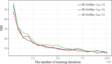
As shown in Fig. 9, a larger population brings mostly negative effects: slow convergence, unstable training, and a poor FID. This confirms our assumption that in the face of a larger population, seems to be a little weak. Therefore, we recommend that the population maintain only one size. More crossover offspring perform relatively well; IE-GAN with reflects the advantage of having a similar number of generative networks as IE-GAN with . This accelerates the convergence, and this IE-GAN’s best FID is comparable to that of a single crossover offspring. This is perhaps due to the excellent crossover operator itself, which improves the fault tolerance of the evaluation. However, probably because of the fast convergence, it appears to experience a bit of overfitting in the late stage. Additionally, it does not observably improve the FID. Considering the increase in the computing overhead due to more generative networks, we choose .
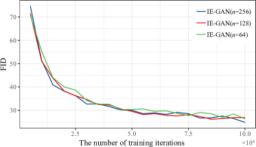
In addition to the total number of individuals evaluated, the survival performance of individuals can also interfere with the fitness of the population. The crossover operator transfers the experience of parental networks using knowledge distillation, and the crossover batch size determines the amount of experience that offspring can access. Logically, the larger is, the more the offspring understands the parental strategy and the better it inherits the superior characteristics. We conduct experiments on this value and record the results in Fig. 10. As expected, the experiments show that the competitiveness of the method is positively correlated with within a certain range. Along with the increase of , IE-GAN improves in terms of the convergence speed, stability, and generative performance. The crossover batch size is set to 256 in this paper; this is consistent with the number of samples used to calculate the fitness value. As mentioned earlier, it is an established practice to evaluate the fitness of mutation offspring before crossover variation. Fully reusing the evaluation results, including the generated samples and single-sample evaluations, can juggle performance and time cost.
The factors affecting the system performance also include , which represents how many samples each sample should be compared with when scoring the diversity. The diversity fitness value, as one of the references for the fitness value, is involved in the selection of surviving individuals for population and learning objects for crossover. Its accuracy is crucial for the effectiveness of the system. The experimental results concerning the value of are listed in Table VI. Experiments show that if this value is too large, this leads to repeated comparisons, thus wasting resources while hindering the reliability of the fitness value. However, if the value of is too small, the samples used to calculate the diversity fitness value cannot be effectively distinguished and does not work. According to the experiments, we think that is appropriate.
| Method | Final FID | Best FID |
| IE-GAN () | ||
| IE-GAN () | ||
| IE-GAN () | 24.82 | 24.82 |
| IE-GAN () | ||
| IE-GAN () |
V-G Diversity Fitness Function Analysis
We explore the effect of the diversity fitness function on the training process on the CIFAR-10 dataset. Fig. 11 shows that is such sensitive to that a small change in value can lead to a reversal in the selected frequency of each operator. This sensitivity forces E-GAN to choose the value carefully. Moreover, E-GAN’s training process is accompanied by the risk of the vanishing gradients problem. When the minimax objective dominates in the early stage (see in Fig. LABEL:sub@fig:SelectedRatew.r.t.Gamma20k), vanishing gradients is difficult to avoid (as shown in Fig. LABEL:sub@fig:SelectedRatew.r.t.Gamma100k). Due to the weakness of the minimax objective in the early stage, the offspring generated by this objective can be easily distinguished by the discriminator. However, gives unreasonably high scores to such distinguishable generators, which leads to the occurrence of the vanishing gradients problem. In contrast, as shown in Table IV, the FID values of IE-GANs varied regularly with the values, indicating that is not overly sensitive to . IE-GANs with various the values all have meaningful results, indicating that does not enhance the possibility of vanishing gradients.
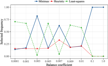
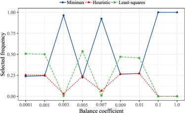
The effect of the diversity fitness function on the generative performance is demonstrated by Table VII. In this experiment, the IE-GANs discard the crossover operator. “w/o ” indicates that only is used for the evaluation. In terms of the generative performance, IE-GAN without the crossover operator and without is equivalent to E-GAN without . The experimental results show that limits and even reduces the performance. By simply removing this costly component, the generative performance of E-GAN can be significantly improved. does not have such an obvious side effect. The degradation of IE-GAN is much smaller than the degradation of E-GAN. The gains of E-GAN due to multiple populations compensate for the negative effect of . Moreover, even maintaining a population of eight individuals, E-GAN is worse than the method that simply uses the quality fitness function. IE-GAN using can outperform IE-GAN using because of the increase in the population.
| Method | Final FID | Best FID |
| IE-GAN / E-GAN (, w/o ) | 27.06 | |
| IE-GAN () | ||
| IE-GAN () | 26.74 | |
| E-GAN () | ||
| E-GAN () |
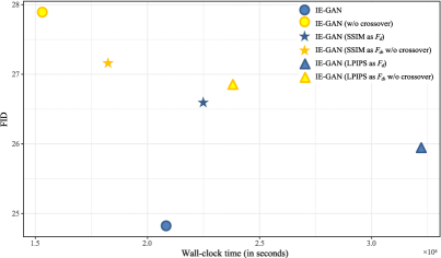
In addition to validating , we have explored other possible options for . Regarding the sample distance measure, in addition to the MAE, we also consider the structural similarity (SSIM) [41] and learned perceptual image patch similarity (LPIPS) [42]. Both are common metrics for measuring the similarity of images. The SSIM imitate human perception by focusing on the similarity of edges and textures. LPIPS extracts features from different layers of a pre-trained model to calculate the similarity of two image inputs. The literature indicates that LPIPS is more consistent with human perception than traditional methods [42]. We use various image similarity measures as diversity fitness functions in the IE-GAN framework. The experiments compare the generative performance and runtime of IE-GAN with different alternative functions. The methods are trained for 100K iterations on the CIFAR-10 dataset. The results are reported in Fig. 12. For fairness, all IE-GANs are grid-searched for and . The adopted hyperparameters are listed in Table VIII.
| Method | ||
| IE-GAN IE-GAN (w/o crossover) | ||
| IE-GAN (SSIM as ) IE-GAN (SSIM as , w/o crossover) | ||
| IE-GAN (LPIPS as ) IE-GAN (LPIPS as , w/o crossover) |
Fig. 12 shows that, in general, a more advanced similarity metric improves the model’s generative performance at the expense of time. In the absence of crossover, the IE-GAN that uses the LPIPS as has the lowest FID. Correspondingly, it has the longest runtime. With the addition of crossover, the LPIPS maintains an advantage over the SSIM in terms of the FID. However, the MAE has a better performance not only in terms of the runtime but also in terms of the FID. Compared to the LPIPS, the MAE has a significant time advantage; compared to the SSIM, the MAE also has better a generative performance. In summary, we finally choose the simple but useful MAE as .
V-H Crossover Operator Analysis
In the implementation of PDERL555https://github.com/crisbodnar/pderl, the -filtered behavior distillation crossover method uses a less capable network as the initial offspring, whereas we choose a better network; this occurs due to the differences between GANs and RL. The networks of GANs tend to be deeper, the generated samples are more time-sensitive, and the sample batch size is smaller to improve the efficiency.
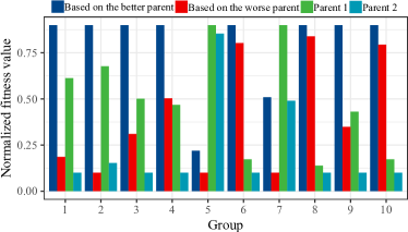
To demonstrate this, we experimentally compare the two crossover operators, i.e., the operator based on the better parent and the operator based on the worse parent. The fitness of the offspring is a good indicator that can be used to measure the quality of the crossover operator. Fig. 13 plots ten randomly selected parent pairs; each set of bars includes the fitness values of the two parents, along with the fitness values of two types of crossover offspring. These values were normalized to [0.1, 0.9]. Not once did the crossover individual based on the worse parent have a higher fitness value than that based on the better parent, and it usually performs worse than the better parent and even the worse parent. It is difficult to assume that the contribution of the poorer individual would exceed that of the better individual. The results in Table IX are consistent with our expectations. A better operator can help the model to be better trained.
| Method | Final FID | Best FID |
| IE-GAN (based on the worse parent) | ||
| IE-GAN (based on the better parent) | 24.82 | 24.82 |
V-I Validation on More Complex Datasets
To demonstrate that our work can be applied to real-world image datasets, in addition to the CIFAR-10 dataset, we also conduct experiments on the CelebA dataset with a DCGAN architecture. In the face of this complex dataset, the network architecture is somewhat weak even with the enhanced number of channels. To maintain the equilibrium between and , in this experiment, we restrict the discriminator update by setting . Six methods are tested: GAN, NS-GAN, LSGAN, GAN-Least-squares, E-GAN and our IE-GAN. Because the discriminator objective functions adopted by IE-GAN are originally used in GAN and NS-GAN, they are just GAN-Minimax and GAN-Heuristic for IE-GAN with . The quantitative results are shown in Table X. All methods are unstable on this dataset, so we only compare the best results. The FID value of the real samples is .
| Method | Best FID |
| GAN-GP (GAN-Minimax) [1] | |
| NS-GAN-GP (GAN-Heuristic) [5] | |
| LSGAN-GP [31] | |
| GAN-Least-squares | |
| E-GAN [6] | |
| IE-GAN (Ours) | 52.582 |
It is clear from the observations that LSGAN essentially fails to be trained and cannot generate meaningful samples. Meanwhile, GAN-Least-squares can be trained, but unlike on CIFAR-10, its performance is the worst out of all the single-mutation-operator methods. E-GAN, as always, does not benefit from multiple operators and performs the worst out of all the trainable methods. Our IE-GAN achieves the best results, and its score is quite close to that of the true distribution. The experiments reveal that IE-GAN has good robustness. It can achieve promising results on different datasets, with different network architectures, and with different operator performances.
VI Conclusion
In this paper, we verify that the evolutionary strategy of E-GAN, especially the diversity fitness function, is unreasonable. We propose a crossover operator that can be widely applied to evolutionary GANs and a more sensible fitness function. We unify them into a universal framework called IE-GAN and implement this framework based on E-GAN and CDE-GAN. Experiments demonstrate that our approach provides a better generative performance and requires less time than previous methods.
References
- [1] I. J. Goodfellow et al., “Generative adversarial nets,” in Proc. NIPS, Dec. 2014, pp. 2672–2680.
- [2] T. Zhang et al., “Generative adversarial network based heuristics for sampling-based path planning,” IEEE CAA J. Autom. Sinica, vol. 9, no. 1, pp. 64–74, 2022.
- [3] J. Li et al., “Predicting lung cancers using epidemiological data: A generative-discriminative framework,” IEEE CAA J. Autom. Sinica, vol. 8, no. 5, pp. 1067–1078, 2021.
- [4] Q. Kang et al., “Effective visual domain adaptation via generative adversarial distribution matching,” IEEE Trans. Neural Networks Learn. Syst., vol. 32, no. 9, pp. 3919–3929, 2021.
- [5] M. Arjovsky et al., “Towards principled methods for training generative adversarial networks,” in Proc. ICLR, Apr. 2017.
- [6] C. Wang et al., “Evolutionary generative adversarial networks,” IEEE Trans. Evol. Comput., vol. 23, no. 6, pp. 921–934, 2019.
- [7] S. Chen et al., “CDE-GAN: cooperative dual evolution-based generative adversarial network,” IEEE Trans. Evol. Comput., vol. 25, no. 5, pp. 986–1000, 2021.
- [8] B. Rozière et al., “Evolgan: Evolutionary generative adversarial networks,” in Proc. ACCV, ser. Lecture Notes in Computer Science, vol. 12625, Nov. 2020, pp. 679–694.
- [9] J. Mu et al., “Enhanced evolutionary generative adversarial networks,” in Proc. CCC, 2020, pp. 7534–7539.
- [10] M. Baioletti et al., “Multi-objective evolutionary GAN,” in Proc. GECCO, Jul. 2020, pp. 1824–1831.
- [11] M. Baioletti et al., “Smart multi-objective evolutionary GAN,” in Proc. CEC 2021, 2021, pp. 2218–2225.
- [12] J. Toutouh et al., “Spatial evolutionary generative adversarial networks,” in Proc. GECCO, Jul. 2019, pp. 472–480.
- [13] Z. Liu et al., “Catgan: Category-aware generative adversarial networks with hierarchical evolutionary learning for category text generation,” in Proc. AAAI, Feb. 2020, pp. 8425–8432.
- [14] V. Costa et al., “COEGAN: evaluating the coevolution effect in generative adversarial networks,” in Proc. GECCO, Jul. 2019, pp. 374–382.
- [15] V. Costa et al., “Exploring the evolution of gans through quality diversity,” in Proc. GECCO, Jul. 2020, pp. 297–305.
- [16] U. Garciarena et al., “Evolved gans for generating pareto set approximations,” in Proc. GECCO, Jul. 2018, pp. 434–441.
- [17] M. Heusel et al., “Gans trained by a two time-scale update rule converge to a local nash equilibrium,” in Proc. NIPS, Dec. 2017, pp. 6626–6637.
- [18] J. Li et al., “Evolutionary generative adversarial networks with crossover based knowledge distillation,” in Proc. IJCNN, Jul. 2021, pp. 1–8.
- [19] G. E. Hinton et al., “Distilling the knowledge in a neural network,” arXiv:1503.02531, 2015.
- [20] Z. Huang et al., “Feature map distillation of thin nets for low-resolution object recognition,” IEEE Trans. Image Process., vol. 31, pp. 1364–1379, 2022.
- [21] M. Li et al., “GAN compression: Efficient architectures for interactive conditional gans,” in Proc. CVPR, Jun. 2020, pp. 5283–5293.
- [22] A. Aguinaldo et al., “Compressing gans using knowledge distillation,” arXiv:1902.00159, 2019.
- [23] C. Bodnar et al., “Proximal distilled evolutionary reinforcement learning,” in Proc. AAAI, Feb. 2020, pp. 3283–3290.
- [24] S. Khadka et al., “Evolution-guided policy gradient in reinforcement learning,” in Proc. NeurIPS, Dec. 2018, pp. 1196–1208.
- [25] I. Gulrajani et al., “Improved training of wasserstein gans,” in Proc. NIPS, Dec. 2017, pp. 5767–5777.
- [26] M. Arjovsky et al., “Wasserstein generative adversarial networks,” in Proc. ICML, ser. Proceedings of Machine Learning Research, vol. 70, Aug. 2017, pp. 214–223.
- [27] J. Adler et al., “Banach wasserstein GAN,” in Proc. NeurIPS, Dec. 2018, pp. 6755–6764.
- [28] N. Yang et al., “Inversion based on a detached dual-channel domain method for stylegan2 embedding,” IEEE Signal Process. Lett., vol. 28, pp. 553–557, 2021.
- [29] A. Jolicoeur-Martineau, “The relativistic discriminator: a key element missing from standard GAN,” in Proc. ICLR, May 2019.
- [30] A. Radford et al., “Unsupervised representation learning with deep convolutional generative adversarial networks,” in Proc. ICLR, May 2016.
- [31] X. Mao et al., “Least squares generative adversarial networks,” in Proc. ICCV, Oct. 2017, pp. 2813–2821.
- [32] A. Brock et al., “Large scale GAN training for high fidelity natural image synthesis,” in Proc. ICLR, 2019.
- [33] T. Karras et al., “A style-based generator architecture for generative adversarial networks,” in Proc. CVPR, 2019, pp. 4401–4410.
- [34] T. Karras et al., “Analyzing and improving the image quality of stylegan,” in Proc. CVPR, 2020, pp. 8107–8116.
- [35] H. Lee et al., “DRIT++: Diverse image-to-image translation via disentangled representations,” Int. J. Comput. Vis., vol. 128, no. 10, pp. 2402–2417, 2020.
- [36] D. Zhou et al., “COutfitGAN: Learning to synthesize compatible outfits supervised by silhouette masks and fashion styles,” IEEE Trans. Multim., 2022.
- [37] D. Zhou et al., “Learning to synthesize compatible fashion items using semantic alignment and collocation classification: An outfit generation framework,” IEEE Trans. Neural Networks Learn. Syst., 2022.
- [38] A. Krizhevsky et al., “Learning multiple layers of features from tiny images,” University of Toronto, Tech. Rep., 2009.
- [39] Z. Liu et al., “Deep learning face attributes in the wild,” in Proc. ICCV, Dec. 2015, pp. 3730–3738.
- [40] V. Costa et al., “Neuroevolution of generative adversarial networks,” in Deep Neural Evolution: Deep Learning with Evolutionary Computation, H. Iba et al., Eds. Singapore: Springer Singapore, 2020, pp. 293–322.
- [41] Z. Wang et al., “Image quality assessment: from error visibility to structural similarity,” IEEE Trans. Image Process., vol. 13, no. 4, pp. 600–612, 2004.
- [42] R. Zhang et al., “The unreasonable effectiveness of deep features as a perceptual metric,” in Proc. CVPR, 2018, pp. 586–595.