Serving DNN Models with Multi-Instance GPUs:
A Case of the Reconfigurable Machine Scheduling Problem

Abstract

Multi-Instance GPU (MIG) is a new feature introduced by NVIDIA A100 GPUs that partitions one physical GPU into multiple GPU instances. With MIG, A100 can be the most cost-efficient GPU ever for serving Deep Neural Networks (DNNs). However, discovering the most efficient GPU partitions is challenging. The underlying problem is NP-hard; moreover, it is a new abstract problem, which we define as the Reconfigurable Machine Scheduling Problem (RMS).

This paper studies serving DNNs with MIG, a new case of RMS. We further propose a solution, MIG-serving. MIG-serving is an algorithm pipeline that blends a variety of newly designed algorithms and customized classic algorithms, including a heuristic greedy algorithm, Genetic Algorithm (GA), and Monte Carlo Tree Search algorithm (MCTS). We implement MIG-serving on Kubernetes. Our experiments show that compared to using A100 as-is, MIG-serving can save up to 40% GPUs while providing the same throughput.

1 Introduction

NVIDIA A100 [10] is the latest and the most powerful GPU launched in 2020. Seemingly, A100 is not cost-efficient for DNN serving (inference) because serving may not fully utilize GPU resources. However, we argue that, equipped with a new feature—Multi-Instance GPU—A100 can be the most cost-efficient GPU ever for DNN serving.

Multi-Instance GPU (MIG) is a new hardware feature introduced by A100. MIG allows people to partition one physical GPU into some number of GPU instances (or instance for short) that are hardware isolated. For example, an A100 can be partitioned up to 7 instances, and each instance has its own processors, memory, L2 cache, and bus bandwidth. Moreover, small instances can be merged into larger instances, for example, two of the 7 instances in A100 (which we call 1/7 instances) can merge to a 2/7 instance with twice the resources.

To understand the serving costs (in dollars) on different GPUs, we calculate how much one needs to pay for serving one request using varied GPUs on AWS [4, 3, 5], including V100, T4, and A100—in which A100 is configured into two variants: using A100 as a whole (A100-7/7) and partitioning A100 into seven 1/7 instances (A100-7$\times$1/7). Figure 1 shows the result: A100-7$\times$1/7 is the most cost-efficient setup for all models.

Can we do better than A100-7$\times$1/7? The answer is yes. We observe that different models have different preferences about instance sizes (§2.2), thus we can improve inference performance by leveraging A100’s heterogeneity; namely, partitioning an A100 into different sized instances, for example, a 4/7 instance, a 2/7 instance, and a 1/7 instance.

Meanwhile, however, heterogeneity improve efficiency at the cost of simplicity. It raises many questions (also opportunities), just to name a few: how to partition GPUs regarding instances of different sizes? Should we mix different models in a GPU, and which ones to mix? DNN service deployers have different throughput and latency requirements for different models (defined as service level objectives, SLOs). Consequently, the GPU configuration that has the highest throughput per resource is not necessarily the best choice. How can we reflect SLOs in the GPU configurations?

All these questions lead to our core question, how to configure MIG-enabled GPUs to most efficiently meet SLOs? By “most efficiently”, we mean that GPUs serving DNN models (called services) can satisfy SLOs with the minimum number of GPUs. Our problem has three characteristics which in combination make the problem novel and challenging.

Figure 1: Normalized cost per request for different DNN models (batch size 8, INT8, TensorRT 7.2) on different GPUs. The cost is calculated based on model serving performance from NVIDIA inference benchmarks [12] and the price from AWS [4, 3, 5].
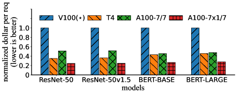
$(\star)$: NVIDIA does not provide inference performance of INT8 for the three leftmost models on V100 [12]; they provide (and we use) “Mixed” precision instead.

First, different DNNs have different performance per resource on different sized instances (§2.2). This means that we cannot simply assume that two 1/7 instances equal one 2/7 instance and assign resources by total amounts, which is a common assumption used by traditional resource allocation algorithms (like allocating CPU cores).

Second, instance allocation is restricted: partitioning GPUs follows specific and (arguably) peculiar rules. These rules may reject seemingly valid partitions. For example, an A100 cannot allocate a 3/7 instance when having a running 4/7 instance, even if it has three free units of resources. This “no $4/7+3/7$” is a hard-coded rule (§2.1), which has something to do with the hardware overhead of MIG [11]. These rules break an assumption made by many resource allocators (like memory and disk allocators) that having $n$ units of free resources indicates one can always allocate a chunk of $n$ resources (by some rearrangements, if needed).

Third, MIG supports partial reconfiguration [45]: a subset of a GPU’s instances can be repartitioned on-the-fly, without affecting other working instances on the same GPU. Partial reconfiguration differs from classic reconfigurable setup (like RMTs [31]) because the amount of resources involved in one reconfiguration is a variable, whereas classic reconfigurable devices, like RMTs, have a basic reconfigurable unit which is fixed in size.

We define an abstract problem, the Reconfigurable Machine Scheduling Problem, that captures and formally specifies the above three characteristics. The problem is NP-hard (§3.3). Despite being computationally expensive to solve, the problem is crucial for deep learning tasks running on MIG-enabled GPUs, as the potential of MIG is enormous. In our experiments, we can save up to 40% GPUs by carefully configuring MIG instead of ignoring MIG and using GPUs as a whole (§8).

This paper describes a system called MIG-serving, which aims at serving DNNs with MIG. MIG-serving takes DNN models and their SLOs as inputs, and produces a set of GPU partitions and service assignments, called a deployment, that satisfies all SLOs and uses as few GPUs as possible.

MIG-serving consists of two main components: optimizer and controller. optimizeris responsible for generating and optimizing deployments. Specifically, it can generate a valid deployment quickly (in minutes); while if more time and computing resources are available, optimizer can gradually improve the result. controlleris in charge of actually applying the deployment to GPU clusters. In the this process, controller ensures that end users will not experience service interruptions.

The contributions of this paper are as follows:

• A study of model serving performance with MIG (§2.2, Appendix B). We study 49 trained models from PyTorch Hub [14] and TensorFlow Hub [15], and evaluate their performances on different sized instances. We observe that the throughput of most models does not grow linearly with the increase of resources.

• Definition of the Reconfigurable Machine Scheduling Problem (§3). We define the problem in theoretical terms to highlight the fundamental difficulties and the relationship to other classic scheduling problems.

• An algorithm pipeline for serving DNNs with MIG (§5, §6). We design a two-step pipeline that explores GPU configurations and searches for cost-efficient deployments, including:

  1. optimizer: balancing two conflicting requirements (§5). optimizerneeds to search for a deployment that satisfies SLOs. Except being computationally expensive, this search has two conflicting requirements in practice: (a) discovering a valid deployment quickly and (b) pursuing the most efficient deployment. We tackle this challenge by a two-phase algorithm that combines two “template algorithms”—a fast algorithm and a slow algorithm—through a tailored Genetic Algorithm (GA).

  2. controller: transparent deployment transition (§6). From time to time, services get updated and optimizer produces new deployments to reflect the changes. controlleris required to execute the deployment transitions transparently—without affecting user experiences. To achieve such transparency, controller uses an algorithm, exchange-and-compact, which guarantees that during transitions, service throughputs are always greater than the required throughputs of the new or old deployments, whichever is smaller.

• A built system and experimental evaluation (§7, §8). We implement MIG-serving on Kubernetes and experiment with it on a 24 A100 GPU cluster. MIG-serving can save up to 40% of GPUs compared to using A100 disabling MIG (§8.1). Also, MIG-serving is able to finish deployment transitions between two real-world workloads within half an hour (§8.2).

2 Multi-Instance GPU

This section introduces MIG in detail (§2.1) and studies the performance characteristics of DNN models running on different sized instances (§2.2). We further describe two straightforward approaches to use MIG for DNN inferences (§2.3), which will serve as baselines in our experiments (§8).

2.1 NVIDIA A100 MIG

MIG is a hardware feature that allows users to partition a GPU into multiple GPU instances (or instance for short). Each instance functions as a traditional GPU. Current A100 GPU implementation has 7 slices of resources and people can organize these resources in many ways with diverse sized instances. For example, a GPU can be partitioned into three instances with 1/7, 2/7, and 4/7 of the total resources respectively. In the rest of the paper, we call an instance with 1/7 of total resources as a 1/7 instance (similarly for instances of other sizes).

Different from resource sharing like MPS (Multi-Process Service), MIG’s instances do not share computational resources: instances have separate streaming multiprocessors (SM), GPU memory, and L1/L2 cache. In addition, instances provide fault and performance isolation by having dedicated on-chip crossbar ports, L2 cache banks, memory controllers, and DRAM address buses. Essentially, an instance is a full-fledged GPU, except some of them are packed in the same “metal box” (an A100).

As mentioned earlier (§1), MIG’s instance allocation follows specific rules; hence having $n$ units of free resources does not imply that a GPU is able to allocate an $n$/7 instance. On the one hand, resources can only be grouped into specific sized instances—1/7, 2/7, 3/7, 4/7, 7/7 instances, whereas others (5/7 and 6/7 instances) are not allowed. On the other hand, the occupied resources also influence the possible allocations. As an example, for a GPU with two running 3/7 instances, allocating a 1/7 instance is prohibited.

Figure 2: Instance allocation rules, borrowed from NVIDIA’s blog [9, Figure 1]. A legal A100 partition picks instances top-down. If an instance is chosen (for example, the shaded 4/7 instance), then all the instances beneath it are unavailable. As an example, the shaded boxes represents a legal partition with a 4/7, a 2/7, and a 1/7 instance.

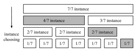
Figure 2 depicts the basic MIG allocation rules. But, there are several exceptions. For example, “3/7 + 4/7” is permitted in the figure but prohibited in practice and “3/7 + 3/7” is possible but not shown in the figure. In total, there are 18 distinct legal instance combinations in one A100 GPU (see the full list in NVIDIA’s document [13]).

Note that the challenge of allocating a larger-than-1/7 instance is different from allocating a chunk of consecutive resources, like memory. If there are $n$ free pages, a memory allocator can always allocate a chunk of consecutive $n$ pages by a series of memory copies. Nevertheless, even a GPU has three available slices, it cannot allocate a 3/7 instance if a 4/7 instance has been allocated, which is a hard-coded rule.

2.2 A study of serving performance with MIG

(a) Model throughputs and latencies of instances of different sizes. The x-axis is the instance sizes, where “1” represents a 1/7 instance, and so on. Bars represent throughputs of the corresponding instances; the solid line represents the 90%-tile latencies. The dashed and dotted lines indicate the throughputs and latencies if the model’s inference performance grows linearly.

(b) Model throughputs and latencies for different GPU partitions. The x-axis is GPU partitions, sorted by throughputs. In x-ticks, digits represent instance sizes, for example, “3-3” represents two 3/7 instances. Bars represent throughputs and lines represent the weighted latencies which is the averages latencies from different instances weighted by their throughputs.

Figure 3: Throughputs and 90%-tile latencies for two PyTorch models, densenet121 and xlnet-large-cased, on different sized instances (Figure 3(a)) and different GPU partitions (Figure 3(b)).

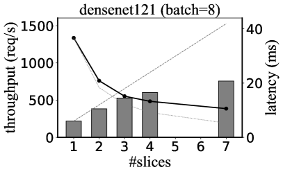
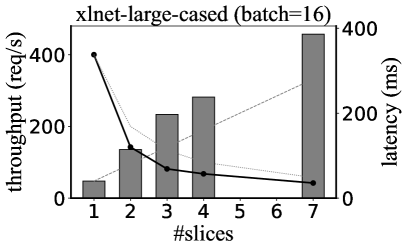
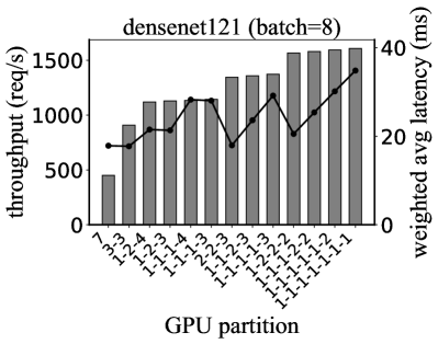
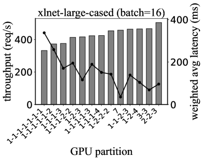
To understand the serving performance on different sized instances, we conduct a study of 49 trained DNNs, in which 24 models are from PyTorch Hub [14] and 25 are from TensorFlow Hub [15] (see Appendix B for all the models). The models are with precision of FP32. We run models on 1/7, 2/7, 3/7, 4/7, and 7/7 instances each for 5 minutes, and collect their throughputs and 90%-tile latencies. Figure 3 shows the results of two PyTorch models—densenet121 and xlnet-large-cased—which represent two categories of models. We use them as illustrative examples below.

By analyzing the throughput and latency trends in Figure 3, we have three main observations:

Observation 1 (Figure 3(a)): the growth of inference throughput is non-linear relative to the increase in resources (i.e., from 1/7 to 7/7 instances). Some models (like densenet121) has sub-linear throughput growth, while others (like xlnet-large-cased) have super-linear throughput growth. Of course, there are models whose throughputs grow linearly (see examples in Appendix B). But the point is, models scale differently, hence a unit of resource contributes differently for different models and instances.

Observation 2 (Figure 3(b)): for the same DNN model, a GPU with different partitions has diverse performance, in terms of throughput and latency. As shown in Figure 3(b), with the same resources (an A100 GPU) but different partitions, throughputs may differ by up to 4$\times$ (for densenet121); the latencies vary up to 8$\times$ (for xlnet-large-cased).

Observation 3 (Figure 3(a), 3(b)): The performance characteristics of different DNN models are different. By pairwise comparing the performance of the two models in Figure 3, we see that models have different performance patterns, and they prefer different GPU partitions. For example, densenet121 prefers small instances, as 1/7 instance has the highest per-unit-throughput without sacrificing too much on the latency—a 20ms latency increase versus an 7/7 instance. On the contrary, xlnet-large-cased should prioritize large instances because they have higher per-unit-throughput and lower latency than smaller instances.

Model performance classification. To understand the performance characteristics across models, we classify models into three categories, based on their throughput growth trends: (1) linear models whose throughputs grow linearly with the increase of computational resources, (2) sub-linear models whose throughputs grow sub-linearly, and (3) super-linear models whose throughputs grow super-linearly.

We classify a model into the three categories as follows. For a model $M$, we calculate a per-unit-throughput for the smallest instance that can run $M$ (usually 1/7 instance, but sometimes 2/7 or 3/7 instance if $M$ is large). Then, we calculate the ratio of 7/7 instance’s throughput and the above per-unit-throughput. If the ratio is within $[6.5,7.5]$, we call $M$ a linear model; if the ratio is smaller than $6.5$, $M$ is a sub-linear model; or else, $M$ is a super-linear model.

Figure 4: Model classifications. “subL”/“L”/“supL” indicate sub-linear/linear/super-linear models, respectively.

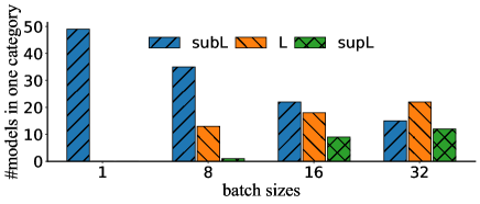
Figure 4 depicts the classification of all 49 models on different batch sizes. We learn that non-linear models are prevalent, which account for majority of the cases. In general, we should assume that a unit of resource contributes differently in different sized instances for most models. Another takeaway is that, when the batch size increases, models are more likely to behave as linear or super-linear. This is intuitive because the larger the batch, the heavier the computation, thus models can saturate (or over-occupy) the hardware resources.

Admittedly, our classification is rudimentary. Comprehensively understanding DNN performance requires further research. Nevertheless, this basic classification sheds some light on interpreting DNN model performance with MIG. Indeed, based on the above observations and classifications, we invent some heuristics which help the performance of our scheduling algorithms (§5.3).

2.3 Strawman approaches: homogeneous partition and static partition

At a high level, serving DNNs with MIG requires first partitioning GPUs into a collection of instances, and then assigning models to instances running as services which respond end user requests. A straightforward approach is to statically partition the GPUs and treat the service assignments as a classic scheduling problem. By whether having heterogeneous instances, we have two baselines as follows.

First, GPUs are partitioned into homogeneous instances (either 1/7 or 7/7 instances), then the problem of scheduling DNN services on instances becomes the Identical Parallel Machine Scheduling Problem [34]. Second, GPUs are partitioned to heterogeneous instances (a mix of multiple instance sizes), thus the problem reduces to the problem of scheduling jobs in a heterogeneous cluster, namely the Unrelated Parallel Machine Scheduling Problem [30, 40].

The two baselines are not ideal as they ignore MIG’s dynamic reconfigurability. Our goal is to design a system that automatically partitions (and re-partitions) GPUs and assigns DNN services to the best suited instances. It turns out that the general problem we face is a new abstract problem, which we define formally in the next section. And, serving DNNs with MIG is a case of this abstract problem. We will circle back with a rigorous problem statement in section 3.3.

3 The Reconfigurable Machine Scheduling Problem

We first defines the Reconfigurable Machine Scheduling Problem (short as RMS) in section 3.1, then highlights the differences between RMS and related scheduling problems in section 3.2. Finally, section 3.3 describes in detail the problem that this paper targets—serving DNNs with MIG.

3.1 Problem definition

We have a set of jobs and a set of machines. Each machine can process one job at a time. Different machines have different processing time for different jobs. Machines are reconfigurable: a set of machines can be rearranged to a different set of machines, under some pre-defined reconfiguration rules (defined below). And the goal is to find a sequence of scheduling and reconfiguration operations that minimizes (or maximizes) some given objective, for example, minimizing cost subject to SLOs [35].

Formally, the problem is defined as follows. There is a set of jobs $\mathcal{J}$ and a set of initial machines $\mathcal{M}_{0}$, where $\mathcal{M}_{0}\subseteq\mathcal{U}_{\mathcal{M}}$ and $\mathcal{U}_{\mathcal{M}}$ is the universe of all possible machines. The processing time of job $j$ on machine $i$ is denoted as $p_{ij}$. We assume that all jobs are known ahead of time and machines do not fail.

A reconfiguration operation ($op_{reconf}$) replaces some machines (say $mset$) in the current machines (denoted as $\mathcal{M}_{k}$) by another set of machines (say $mset^{\prime}$). The $op_{reconf}$ does not affect jobs running on machines other than $mset$, which is $\{m_{j}|m_{j}\in\mathcal{M}_{k}\land m_{j}\not\in mset\}$. We call the available machines after a reconfiguration $\mathcal{M}_{k+1}$ and $\mathcal{M}_{k+1}=(\mathcal{M}_{k}\setminus mset)\cup mset^{\prime}$ because $mset^{\prime}$ replaces $mset$.

reconfiguration rules (denoted as $rule_{reconf}$) specify whether an $op_{reconf}$ is legal. For example, whether two machines can be merged into a larger machine (an analogy to the rule of merging two consecutive 1/7 instances, Figure 2). Note that the contents of $rule_{reconf}$ are specific to problems and are not part of the RMS definition. As an example, for serving DNNs with MIG, reconfiguration rules follow MIG partition rules. The definition of $rule_{reconf}$ is:

$$rule_{reconf} (mset,mset^{\prime},\mathcal{M}_{k})\ \to\ Boolean,$$

$$\textrm{where }mset\subseteq\mathcal{M}_{k}\ \land\ mset,mset^{\prime}\subseteq\mathcal{U}_{\mathcal{M}}$$

We say a reconfiguration operation $op_{reconf}(mset,mset^{\prime})$ is legal, if and only if $rule_{reconf}(mset,mset^{\prime},\mathcal{M}_{k})$ returns $True$.

Fitting into the scheduling framework. RMS can be described by the classic scheduling framework [40], as a triplet $(\ \alpha\ |\ \beta\ |\ \gamma\ )$. The $\alpha$, $\beta$, and $\gamma$ are three pieces of information characterizing a scheduling problem:

• $\alpha$ indicates the machine environment. For example, unrelated machine in parallel ($R_{m}$) is one type of $\alpha$ in which machines run in parallel and different machines process different jobs at different speeds.

• $\beta$ describes processing characteristics and constraints, for example, preemption.

• $\gamma$ represents the objective to minimize (or maximize), for example, minimizing total cost regarding SLOs ($Cost_{min}$).

We see machine reconfigurability ($op_{reconf}$ and $rule_{reconf}$) as a member of $\beta$ field, and we denote it as $reconf$. Thus, RMS can be simply read as:

$$(\ R_{m}\ |\ reconf\ |\ *\ ).$$

The above asterisk ("$*$") indicates that RMS’s objectives are subjective to change for different problems. For example, with $\gamma=Cost_{min}$, the problem becomes searching for a series of scheduling and reconfiguration operations that minimizes the cost while preserving SLOs. This problem $(R_{m}|reconf|Cost_{min})$ is the focus of this paper (detailed description in §3.3)

3.2 Related scheduling problems

Scheduling is a broad topic that has been intensively studied. There are prior scheduling problem variants that consider reconfiguration in several forms [31, 28, 23, 48, 33, 16, 27], but none of them fully captures the characteristics of MIG. We elaborate the most relevant ones below (see more in §9).

A recent work that is closely related to our problem (RMS) is FJSSP-CDST [33] (Flexible Job Shop Scheduling Problem with machine Configuration-Dependent Setup Times). This is a problem combining a classic scheduling problem FJSSP [39, 40] and a module named RMTs [31] (Reconfigurable Machine Tools). An RMT is a fixed group of machines that can be deployed with different configurations to serve multiple manufacturing purposes.

RMS differs from FJSSP-CDST in the way how reconfigurations behave. FJSSP-CDST has a basic reconfigurable unit (an RMT) which contains a fixed group of machines. During a reconfiguration, all machines in this unit have to stop. This is a restriction to our (hence MIG’s) reconfigurability because we do not dictate which machines have to be reconfigured at the same time; for example, an A100 GPU can merge two 1/7 instances without affecting other instances.

Other related scheduling problems include DCSP [23, 28] (Discrete-Continuous Scheduling Problem) and UPM [40, 30] (Unrelated Parallel Machine Scheduling Problem). The former, DCSP, studies the continuously divisible resources (for example, power), whereas resources in GPUs are discrete (organized and exposed in instances) and are constrained in allocation—for example, allocating a 3/7 instance requires no 4/7 instance in the same GPU. For the latter, RMS shares the same machine environment ($R_{m}$) with UPM, but UPM does not consider machine reconfigurations.

3.3 A case of RMS: serving DNNs with MIG

This paper focuses on a variant of RMS—serving DNNs on GPUs with MIG. In this problem, machines are GPU instances; jobs are DNN services; different services have different performance on different sized instances (DNNs’ non-linear performance, §2.2). A set of instances in one GPU can be re-partitioned to another set of instances (a reconfiguration), without affecting other running instances on the same GPU. Our goal is to find the most efficient GPU partitions and service assignments that minimizes the number of GPUs used.

A reconfiguration is valid when it follows the MIG partition rules (§2.1), defined below.

$$rule_{reconf} (mset,mset^{\prime},\mathcal{M}_{k})\triangleq$$

$$\ \ \ \ \forall m\in mset\cup mset^{\prime},\ m\textrm{ is in the same }GPU_{i}$$

$$\land\mathcal{M}_{k}|_{GPU_{i}}\in\textrm{legal A100 partitions}$$

$$\land\mathcal{M}_{k}|_{GPU_{i}}\setminus mset\cup mset^{\prime}\in\textrm{legal A100 partitions}$$

In the above definition, $mset$ and $mset^{\prime}$ are GPU instances before and after the reconfiguration. The reconfiguration succeeds iff all instances in $mset$ and $mset^{\prime}$ are from the same $GPU_{i}$, and the GPU partitions before and after reconfiguration ($\mathcal{M}_{k}|_{GPU_{i}}$ and $\mathcal{M}_{k}|_{GPU_{i}}\setminus mset\cup mset^{\prime}$) are legal A100 partitions.

One characteristic of serving DNNs is that jobs (services) are “long-running”: they do not finish until a shutdown or an update. This is a simplification compared to the general RMS because it spares the decisions on job scheduling timing. In particular, we do not have to consider when to schedule a job (service) because they all need to be deployed in the beginning and are long-running.

Serving DNNs with MIG is an NP-hard problem because an NP-hard problem, Cutting Stock Problem [6], reduces to it. The cutting stock problem studies how to cut standard-sized paper rolls into certain numbers of specified-sized pieces while minimizing wasted material. This problem can reduce to our problem by treating the paper rolls as GPUs, specified-sized pieces as different sized instances for services, and the required piece numbers as SLOs. If one can find the minimum GPUs for our problem, we know the minimum paper rolls for the original problem, which minimizes the wasted materials.

4 System overview

To serve DNNs with MIG efficiently, we design and implement a system, MIG-serving, which automatically partitions GPUs and assign services. This section introduces MIG-serving’s design and its main components: optimizer and controller.

Figure 5: MIG-serving’s architecture.

Workflow. Figure 5 depicts MIG-serving’s architecture.

A service deployer specifies what services (DNN models) to run and their service-level objectives (SLOs) which include required throughputs and expected latencies.

MIG-serving takes in the services (models) and their SLOs as inputs, and is responsible to produce a deployment—a combination of GPU partitions and service assignments. A deployment is valid if it satisfies SLOs: for each service, (i) the sum of throughputs from all instances is greater than the required throughput, and (ii) the 90%-tile latency of each instance is smaller than what required by SLOs.

MIG-serving then generates a transition plan which transfers GPU clusters from the current deployment to the newly generated one. Finally, MIG-serving executes this transition plan on GPU clusters. The entire transition process is transparent to end users; they do not experience service interruptions.

MIG-serving has two main components, optimizer and controller. At a high level, optimizer designs a valid deployment for the given SLOs, and controller implements this deployment transparently. Next, we briefly introduce these two components.

optimizer. optimizertackles the optimization problem of serving DNNs with MIG (§3.3): finding a valid deployment that uses as few GPUs as possible. optimizerruns a two-phase algorithm which blends a heuristic greedy algorithm, a Genetic Algorithm (GA), and a Monte Carlo Tree Search algorithm (MCTS). The first phase aims at finding a candidate deployment which is valid but suboptimal in terms of GPU usage efficiency. The second phase improves the candidate deployment via a combination of custom-designed GA and MCTS.

This two-phase design is crucial in practice because it balances two important but conflicting requirements: (i) getting a valid deployment quickly and (ii) taking full advantage of every single GPU. The two requirements are at odds because we need to quickly have at least some plan that satisfies the SLOs in case of urgent changes, but exploring configuration possibilities takes a lot of time.

optimizer’s first phase runs a fast algorithm (the heuristic greedy algorithm) in $O(n^{2}m)$ where $n$ and $m$ is the number of services and GPUs, which can produce results in minutes; whereas the second phase is expensive and runs continuously and massively in parallel. Note that the second phase is on-demand. People can decide how much time and how many computational resources they are willing to devote.

controller. controllerreceives two inputs, the new deployment (from optimizer) and the current deployment on GPU clusters. controller’s duty is to (i) plan a series of actions (called a transition plan) that switch GPUs from the current configurations to the new version, and (ii) execute the transition plan without affecting user experiences.

To achieve the above goals, controller runs an algorithm, called exchange-and-compact. At a high level, the algorithm first changes current service instances to the wanted sized instances while maintaining the required throughputs during this process, with the help of extra GPUs; it then repartitions GPUs and packs the services into the planned number of GPUs.

During a deployment transition, controller has four types of actions: instance creation, deletion, migration, and GPU repartition. These actions are implemented in Kubernetes (§7), and controller issues actions according to the transition plan, and some actions are issued in parallel (§6).

5 optimizeralgorithm

This section describes how MIG-serving solves an optimization problem of minimizing number of GPUs used while satisfying SLOs. Section 5.1 encodes this optimization problem; section 5.2 depicts the overall algorithm pipeline of MIG-serving’s optimizer; and section 5.3 introduces the two concrete algorithms optimizer uses.

5.1 Defining optimizer procedure

As mentioned (§4), optimizer is obligated to generate valid deployments that fulfill SLOs. Next, we define this procedure, which provides a basic framework for different algorithms.

optimizer’s inputs are (1) service performance (throughput and latency) on different sized GPU instances (1/7–7/7 instances), and (2) SLOs which include required throughputs and latencies for each service. optimizer’s output is a deployment that consists of GPU partitions and service assignments.

We define completion rates for a deployment to represent the deployment’s progress of satisfying SLOs. completion rates is a vector of percentage numbers; each number represents the percentage of a service’s current throughput to the required throughput in SLOs. For example, a deployment has completion rates of $[0\%,100\%,\cdots]$ means that the deployment does not run $\textrm{service}_{0}$ on any GPUs while $\textrm{service}_{1}$ is fully satisfied.

For a service running on an instance, we calculate a utility which indicates how much this instance contributes to the service’s total throughput requirement. For example, if $\textrm{service}_{0}$ requires $1000$ req/s and a 1/7 instance has a throughput of $50$ req/s for $\textrm{service}_{0}$, then we say $\textrm{service}_{0}$ on 1/7 instance has a utility of $[+5\%,0\%,\cdots]$ (we use “$+$” to distinguish utility from completion rates). With the utilities of all services, we can calculate the utility for a GPU by adding up the utilities of all instances in this GPU: for the same example of $\textrm{service}_{0}$, if a GPU has seven 1/7 instances running $\textrm{service}_{0}$, it has a utility of $[+35\%,0\%,\cdots]$ ($35\%=7\times 5\%$).

Note that the utility space for all possible GPU configurations is enormous. A loose upper bound is $O(n^{7})$ where $n$ is the number of services, because a GPU has at most $7$ instances and each instance can run one of $n$ services. Of course, the actual size is much smaller than this bound. Nevertheless, it is still huge; the number of possible GPU configurations (utilities) is 157.8k and 234.7k when $n$ is 12 and 13, respectively.

Finally, we define an optimizer procedure as follows. Given (i) utilities for all service on all sized instances and (ii) completion rates, an optimizer procedure should produce a set of GPU configurations, such that the sum of all GPU configuration utilities and the completion rates must be greater than or equal to $[100\%,100\%,...]$ (with respect to vector comparison). Note that the given completion rates is not necessarily all zeros.

5.2 Two-phase algorithm and GA

Figure 6: MIG-serving’s two-phase algorithm. The fast algorithm and the slow algorithm are optimizer procedures (§5.1).

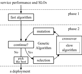
MIG-serving’s optimizer runs a two-phase algorithm, which is outlined in Figure 6. It has two “template” algorithms, namely the fast algorithm and the slow algorithm. Both template algorithms must be an optimizer procedure (§5.1), and the fast algorithm is supposed to run (relatively speaking) fast. The two algorithms are connected by the two-phase design and a custom-designed Genetic Algorithm (GA for short). In the rest of the section, we first introduce the properties of the fast and the slow algorithms, and then describe the custom GA and its two main pieces, crossover and mutation.

Fast and slow algorithms. In our design, we require the fast algorithm (i) to be a legal optimizer procedure, and (ii) running fast—the algorithm’s time complexity must be polynomial with respect to the number of services and GPUs. In practice, we require the algorithm to finish in minutes.

For the slow algorithm, we only require it to be a legal optimizer procedure. Nevertheless, we expect the slow algorithm to discover better solutions than the fast algorithm (hopefully in high probability). This expectation ought to be possible as the slow algorithm is given more time budgets.

In MIG-serving, we use a heuristic greedy algorithm as the fast algorithm, and Monte Carlo Tree Search (MCTS) as the slow algorithm (§5.3). Of course, they are changeable.

GA overview. GA is a heuristic algorithm framework inspired by nature gene evolution. We tailor GA to our context: a chromosome is a deployment, and genes are GPU configurations. To evolve, a chromosome (deployment) conducts crossovers and mutations. A crossover erases some GPU configurations in a deployment and fills in with new GPU configurations generated by the slow algorithm. A mutation swaps services running on instances in a deployment.

GA runs in rounds. In each round, we select the best deployments in the last round, and let them attend the coming crossovers and mutations. GA stops when time out, or the best deployment stops improving in the past ten rounds. Note that GA keeps the original deployments in each round’s comparison, so that the best candidate only improves over time.

Crossover. A crossover applies to a (valid) deployment, which contains two steps. First, we randomly erase some GPU configurations, which decreases the overall throughputs and makes some services unsatisfied. As a result, we have completion rates that are not all-$100\%$. Second, we run the slow algorithm against the current completion rates and get a deployment that makes up for the previously erased GPUs. The figure below is an illustrative example. Each rectangle represents an instance; and different colored symbols (e.g., stars, triangles, squares) represent different services.

The insights behind this crossover approach are twofold. First, a crossover mixes solutions from the slow algorithm and the fast algorithm, thereby providing diversity. Second, the problem size of crossovers is much smaller than the original one, hence the slow algorithm can finish in reasonable time.

Mutation. Mutation is based on an observation that DNN inference does not have affinity requirements (different from DNN training); that is, instances of the same size are identical for inference. A mutation randomly picks some instance pairs; each pair contains two instances that are the same in size but run different services. The Mutation then swaps the services in each pair. The figure below depicts this process.

The idea of mutation is to explore different combinations of services on one GPU. Mutations themselves do not improve deployments. But they create diverse service mixing on GPUs which helps crossovers explore combining different services.

5.3 Algorithm, fast and slow

In this section, we introduce the fast and the slow algorithms used in MIG-serving. The two algorithms are chosen from a pool of candidate algorithms. It is possible that we may find better algorithms in the future. MIG-serving is designed to be able to switch algorithms easily.

Fast algorithm: heuristic score and greedy algorithm. MIG-serving develops a greedy algorithm as the fast algorithm, which chooses the “best” GPU configurations according to a heuristic score. This score represents how well a GPU configuration serves the current service requirements, that is the complementary to the current completion rates (namely, $\mathbbm{1}-$ completion rates, where $\mathbbm{1}$ is an all-1 vector).

The greedy algorithm works as follows. First, it ranks the known GPU configurations by their scores and picks the one with the highest score. The algorithm then updates the completion rates and repeats the above step until all service throughputs reach or exceed SLOs. (Appendix A.1 describes this heuristic greedy algorithm in detail.)

The heuristic score of a GPU configuration is based on two factors: the current completion rates (a vector of percentages, §5.1) and the GPU configuration’s utility (a vector of percentages, §5.1). Below is the score’s definition, where $c_{i}$ and $u_{i}$ are the $i_{th}$ number in the completion rates and the utility, respectively; $\mathbbm{1}$ is an all-1 vector; $n$ is the number of services.

score(config) $$=\sum(\mathbbm{1}-\textrm{completion rates})\odot\textrm{config's utility}$$

$$=\sum_{0}^{n-1}(1-c_{i})\times u_{i}$$

The idea behind the score is to balance a GPU’s overall throughputs and the current service needs. On the one hand, higher throughputs are likely to have higher scores. On the other hand, the GPU configurations which contribute to services with low completion rates are likely to have higher scores. For example, if a configuration $config_{a}$ has higher throughputs than $config_{b}$, then $config_{a}$ has a higher score. However, if all services that $config_{a}$ contributes to are fully satisfied, then the throughputs don’t count and $config_{a}$’s score is $\mathrm{\Gamma }$.

Slow algorithm: MCTS. MIG-serving tailors the Monte Carlo Tree Search (MCTS) as the slow algorithm. We choose MCTS because the problem of allocating MIGs can be naturally encoded to a tree search problem; hence MCTS, as a well-studied tree search algorithm, is a good candidate.

Figure 7: An example tree for the problem of serving DNNs with MIG. The nodes (denoted as $C_{i}$) represent completion rates, and $C_{m}$ is a leaf node. Edges (denoted as $U_{j}$) represent utilities of GPU configurations.

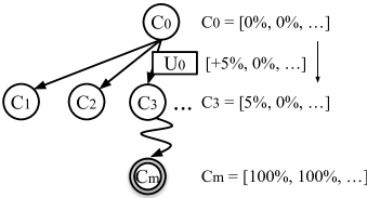
Figure 7 depicts an example of the tree search problem. Nodes represents completion rates. Edges represents GPU configuration’s utilities. A transition from a parent node to a child represents the MIG-serving picking a GPU configuration (indicated by the edge). Leaf nodes are nodes whose completion rates are all-100% (or larger than 100%), meaning that all services are satisfied. The goal is to find the shortest path from the tree root (the initial completion rates) to a leaf node. This shortest path is the deployment that uses the minimal number of GPUs (the length of the path).

MCTS is designed to search heuristically and find a good solution. However, vanilla MCTS doesn’t work in our problem, for two reasons. First, each node has too many children: the number of children equals the number of edges, which equals the number of GPU configurations. As mentioned earlier (§5.1), the configuration space is huge. Second, the classic MCTS estimation procedure (also known as simulation, playout, or rollout) is slow and inaccurate. The original estimation is to find a random path to some leaf node which is used to estimate the depth of a subtree. However, our problem requires an estimation of the shortest path instead of a random path, which leads to an extremely inaccurate estimation.

To address the above two problems, MIG-serving customizes MCTS by (i) cutting the children of each node into the nodes with the top-K heuristic scores (K=10 by default) and (ii) using a fast-and-accurate estimation via memoization and randomization. The details of the custom MCTS are described in Appendix A.2.

6 controller algorithm

MIG-serving targets the real-world serving environment, in which SLOs change from time to time, for example, a shift from daytime to night. In addition, services get updated as well—adding/removing services and upgrading DNN models. In the above cases, MIG-serving needs to recalculate deployments to adapt to the new requirements, and transfer GPU clusters from the old deployment to the new one. We call this process a deployment transition.

In MIG-serving, controller is responsible for designing and implementing deployment transitions (see Figure 5). A straightforward transition approach is to shut down all services, repartition underlying GPUs, and then reboot the services. Of course, this method is unacceptable in practice because services are unavailable during transitions.

The goal of controller is to finish a transition without interrupting user experiences and finish it quickly. controller introduces an algorithm, exchange-and-compact, which uses two phases to achieve the aforementioned goals.

Exchange phase. Two deployments differ in two factors: instance sizes for services and GPU partitions. Exchange phase addresses the first factor by creating and deleting different sized instances. First, controller calculates the instance differences between the old and the new deployments for each service. We denote the difference as $\Delta_{i}$ for $\textrm{service}_{i}$, which contains the “diff” of $\textrm{service}_{i}$’s instances. For example, a $\Delta_{i}=[+4/7,-2/7]$ means that $\textrm{service}_{i}$ requires a new 4/7 instance and has an unneeded 2/7 instance.

For each service, controller pairs every new instance (for example, “$+4/7$”) with some unneeded instances (for example, “$-2/7$”) such that the throughputs of the new instance is equal to or larger than the unneeded instances. Note that pairing an unneeded instance which has larger throughputs is not allowed (for example, pairing “$+1/7$” and “$-7/7$”) because that may fail providing the adequate throughputs hence affecting user experiences. Finally, controller has a set of new-unneeded instance pairs and a list of unneeded instances that cannot pair with any new instances.

controller executes each new-unneeded instance pair by creating the new instance first (using extra GPUs if needed) and then deleting the unneeded instances. After finishing all pairs, controller deletes instances in the unneeded list. During the entire process, controller guarantees that services have enough capacity to handle the expected volume of user requests.

Compact phase. After the exchange phase, all services have the wanted sized instances in the new deployment. But the GPU partitions haven’t been changed yet, and controller uses more GPUs (i.e., extra GPUs) than expected because of GPU instance fragmentation. In the compact phase, controller defragments GPUs by repartitioning GPUs and migrating instances.

At the beginning of this phase, controller creates a list of GPUs which are not fully occupied (having unused instances), denoted as $S$. If $S$ is not empty, controller picks a $GPU_{i}\in S$, and gathers some running instances from other GPUs in $S$ such that these instances together can fully occupy $GPU_{i}$; controller repartitions $GPU_{i}$ (if needed), migrates these instances to $GPU_{i}$, and removes $GPU_{i}$ from $S$ (the $GPU_{i}$ is now fully utilized). controller continues the above process until achieving the new deployment.

Optimizations. controller adopts several optimizations. We list two below. First, controller is locality-aware—it prioritizes local instance migrations over cross-machine migrations. In our GPU clusters, each machine has 8 A100 GPUs; migrating instances within a machine is much cheaper than migrating across machines. Second, actions can run in parallel if the affected GPUs are separate. controller analyzes the dependencies between actions and executes the non-conflicting ones simultaneously.

Note that the exchange-and-compact algorithm can happen in different granularities, depending on how many extra GPUs available. If there are many, controller can run exchange-and-compact once for all services. However, if only few extra GPUs are available, controller will run exchange-and-compact in multiple rounds; in each round, controller only targets a small number of services.

7 Implementation

MIG-serving is implemented in Python and Kubernetes (k8s). Figure 8 lists the components of MIG-serving implementation. For optimizer, we implement the optimizer procedure (§5.1) as an abstract class that the fast and the slow algorithms extend. MIG-serving can easily switch to other algorithms by implementing them under the same abstract class.

We implement controller by extending k8s controller [8]. MIG-serving’s actions—instance creation, deletion, migration, and GPU partition—are wrappers of k8s operations. For example, a remote instance migration from machine $A$ to $B$ is a sequence of operations: creating an instance on machine $B$, checking if the instance on $B$ is successfully launched, and deleting the instance on machine $A$.

MIG-serving always chooses the largest batch sizes possible, as far as the inference latency is smaller than what required by SLOs. This may result in a service with different batch sizes for different instances. MIG-serving relies on load balancing systems to dispatch user requests accordingly.

MIG-serving component	LOC
optimizer
data structures	2674
fast algorithm (greedy)	135
slow algorithm (MCTS)	398
Genetic Algorithm (GA)	330
controller
k8s controller	1318
exchange-and-compact algorithm	319

Figure 8: Components of MIG-serving implementation.

8 Experimental evaluation

In this section, we answer three questions:

• How many GPUs does MIG-serving save, versus baselines?

• How long does MIG-serving take to complete a deployment transition, and what components cost the most?

• Do MIG-serving’s deployments meet SLOs in practice?

Baselines and workloads. We have three baselines with static GPU partitions: (1) A100-7$\times$1/7, partitioning GPUs into 1/7 instances, (2) A100-7/7, using A100 GPUs as-is, and (3) A100-MIX, partitioning all A100 into “4-2-1” (a combination of 4/7, 2/7, and 1/7 instances) and scheduling one service on one GPU. A100-7$\times$1/7 is the most cost-efficient setup as shown in Figure 1. A100-7/7 uses GPU the traditional way (ignoring MIG). A100-MIX represents heterogeneous setup but ignoring the characteristics of workloads.

To see how well MIG-serving performs compared to the optimal solution (which is computationally expensive to have), we calculate an approximate optimality—a lower bound of GPU usage by ignoring MIG’s hardware constraints. In particular, we assume that any combination of instance is possible, and the minimal number of GPUs can be calculated by always using the most cost-efficient instance. Notice that the lower bound is likely impossible to achieve due to ignoring the hardware constraints.

We uses two sets of workloads in the following experiments:

• Simulation workloads (requiring hundreds of GPUs): we generate four workloads for 24 DNN models. In each workload, models’ SLO throughputs are generated from either normal distributions (for two workloads) or lognormal distributions (for the other two workloads). The latencies in SLOs are set to 100ms, which is an acceptable waiting time under most scenarios.

• Real-world workloads (requiring up to 16 GPUs): we build two real-world workloads for five DDN models running in our GPU clusters. We collect 24-hr production throughputs of the five models and construct the workloads: one workload represents the peak throughputs (called daytime workload), and the other workload represents the low throughputs (called night workload). Note that we scale down models’ throughputs to fit into our testbed which has 24 A100 GPUs, while preserving throughputs’ relative amounts.

We run MIG-serving on a 104-core machine with 750G memory running Debian 9.13. To test real-world workloads, we have a three-machine GPU cluster with 24 A100 GPU cards (8-GPU for each machine). The five DNN models for the real-world workloads are robert-large, bert-base-uncased, albert-large-v2, resnet101, and resnet50.

8.1 optimizeralgorithms

In this section, we study how many GPUs MIG-serving saves compared to baselines. The workloads used are the four simulation workloads generated from normal and lognormal distributions, denoted as normal-1, normal-2, lognormal-1, and lognormal-2. We design the four workloads to use several hundreds of GPUs, representing a median-sized GPU cluster.

Figure 9: Number of GPUs used by algorithms for different workloads. The numbers are normalized clusterwise for each workload. MIG-serving’s absolute numbers of GPUs used are given. “A100-7/7”, “A100-7$\times$1/7”, and “A100-MIX” are the three baselines; “greedy” represents MIG-serving’s fast algorithm (§5.3); “MIG-serving” represents optimizer’s two-phase algorithm; “lower-bound” is the minimal number of GPUs ignoring MIG’s hardware constraints.

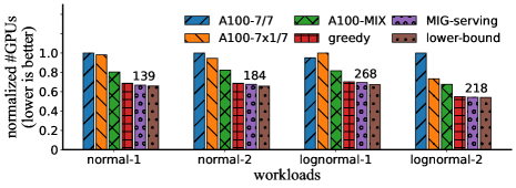
GPU saved. We run MIG-serving and the baselines on the simulation workloads and count the number of GPUs they use. Figure 9 shows the results. MIG-serving uses fewer GPUs than other baselines. It saves up to 40% GPUs compared to A100-7/7. Moreover, MIG-serving is close to the optimal allocation—MIG-serving uses $<$3% more GPUs than the GPU lower bound (the “lower-bound” in Figure 9). One thing to clarify is that A100-7$\times$1/7 does not perform as well as in Figure 1 because solutions now consider latencies, hence some models cannot use large batch sizes on 1/7 instances.

Note that this experiment does not consider the running time of algorithms. Thus, it is not an entirely fair comparison because baselines finish in seconds, whereas MIG-serving’s fast algorithm finishes in minutes and the optimizer’s two-phase algorithm finishes in hours (MIG-serving runs 10 rounds of GA for the four workloads and finishes in 3hr, 5hr, 6.5hr, and 6hr). But in practice, the service and SLO updates are relatively infrequent (for example, twice a day), thus we can afford to run optimizer’s two-phase algorithm. In addition, the deployment can be reused if models and their SLOs are not changed.

Figure 10: Normalized costs for satisfying SLOs of different workloads. “A100-7/7” and “A100-7x1/7” are the two baselines (with A100); “T4” represents using T4 GPUs; “MIG-Serving” repreesnts the two-phase algorithm with A100. We use the price from AWS GPU machines [3, 5].

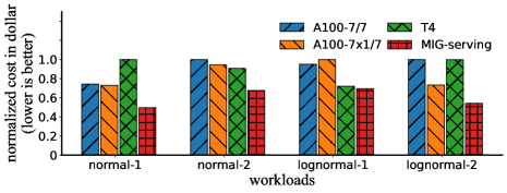
Cost versus T4. To compare the cost-efficiency with other GPU types, we evaluate how many T4 GPUs the simulation workloads need to satisfy their SLOs. We choose T4 because it is the most cost-efficient GPU type for DNN serving before A100. Figure 10 shows the results. MIG-serving is the most cost-efficient configuration for all workloads.

Figure 11: The ratio of GPU saved compared to using A100 as-is (“A100-7/7”) with different MPS configurations. The left four bar clusters represent the GPUs saved with no MPS; the middle four represent the configuration with at most two MPS processes in each instance; and the last four with at maximum four MPS processes.

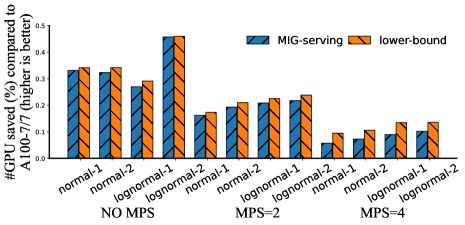
Combining MIG and MPS. MIG and Multi-process service (MPS) are orthogonal techniques that can be used together. With MPS, multiple processes can share the same GPU, which applies to GPU instances generated by MIG. We combine MIG and MPS by running up to $N$ processes of the same model in one GPU instance (e.g., 1/7 instance). In our experiments, we use $N=2,\,4$ because we experienced out-of-memory exceptions when $N>4$.

Figure 11 shows the ratio of GPU saved compared to the baseline A100-7$\times$1/7. By using MPS, multiple processes share GPU resources, and the GPU utilization increases. Hence, the baseline, A100-7$\times$1/7, has better performance and the GPUs saved by MIG-serving are not as many. When using four MPS processes, MIG-serving saves about 10% GPUs. Nevertheless, MPS increases GPU utilization at the cost of tail latency stability and failure isolation. Since MPS has no memory and failure isolation, using it may cause unexpected high tail latency and correlated failures among model processes. Deciding whether to use MPS and how many processes to run is a trade-off that users need to make.

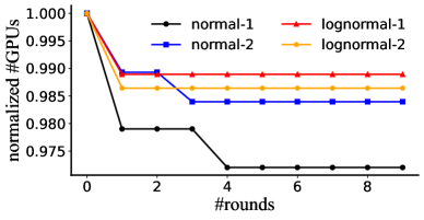
Slow algorithm improvement. We study how the slow algorithm improves over the fast algorithm by running 10 rounds of GA and MCTS. Figure 12 depicts the improvements for each round. We can see that MCTS improves the solutions of the heuristic greedy algorithm by saving 1–3% GPUs, which is much minor than we expected. However, it is still worthwhile: we can save several to dozens of GPUs by spending multiple CPU hours. One of our near future work is to tune GA and MCTS to further improve the deployments.

Figure 12: The improvement of the slow algorithm (MCTS) over the fast algorithm (heuristic greedy) on each GA round. Each line represents a simulation workload. The number of GPUs required is normalized to the original deployment (round 0 of the fast algorithm). Notice that the y-axis starts at 0.97.

(a) End-to-end runtime of deployment transitions and time spent on different components.

(b) Number of actions during transitions.

(c) Runtime of (synchronous) MIG-serving actions. Bars are average runtime of 10 runs. Error bars indicate the maximum and minimum runtime.

Figure 13:

8.2 deployment transition

We run MIG-serving on our testbed for the two real-world workloads (the daytime and night workloads), and experiment with deployment transitions between the two workloads. In particular, we first deploy the five services from the daytime workload, which uses 16 GPUs. Then, we instruct MIG-serving to switch the deployment to the night workload, which uses 5 GPUs for the same services. We call this transition, day2night. Likewise, we call the other way around, night2day.

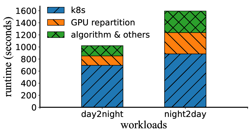
End-to-end transition runtime. We measure the wall-clock time of MIG-serving’s two deployment transitions, day2night and night2day. Figure 13(a) shows the results. The transition of day2night is faster than night2day because the former is mostly shrinking services and reducing the number of GPUs, whereas the latter requires expanding services and increasing GPUs.

We further decompose each transition runtime into time spent on different components: k8s, GPU partition, and the exchange-and-compact algorithm. We find that k8s takes the majority of the time. By profiling, it turns out that most of k8s’ runtime is spent on bootstrapping an instance (a k8s pod) on certain GPUs. We believe DNN context switch techniques, like Pipeswitch [17], can significantly reduce this overhead.

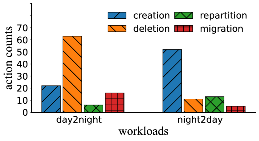
A closer look at transitions. To understand the details of the two transitions, we record the actions issued by MIG-serving during day2night and night2day, and summarize them in in Figure 13(b). The day2night transition issues more instance deletions, while night2day has more instance creations. This is because the deployment during daytime requires more throughputs (hence instances) than the deployment during night. Also, night2day has more GPU partition actions because this transition involves more GPUs, which need to be configured into the planned partitions.

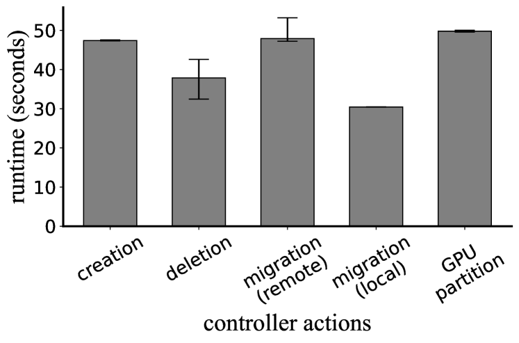
controlleractions. As mentioned earlier (§4), controller has four types of actions, instance creation, deletion, migration (local and remote), and GPU partition. We measure each of their runtime and show results in Figure 13(c). Note that we run these actions in a synchronous manner—we issue an action and wait until it finishes. In practice, all these actions are asynchronous and issued in parallel. MIG-serving only has to wait when the actions have dependencies, for example, creating a replacement instance before deleting an old instance.

8.3 Serving requests in practice

To understand whether MIG-serving’s deployments satisfy SLOs, we run the two deployments across models, under the two real-world workloads, on our testbed and measure their throughputs in practice. For each deployment, we run multiple inference clients that continuously issue requests to DNN services deployed by MIG-serving. To saturate DNN services, clients gradually increase the number of requests per second until the throughput reaches its maximum. In the following, what we report is the maximum throughputs. Clients and DNN services run on different machines which are connected by 10Gbps datacenter networks.

Figure 14: Throughputs required by SLOs versus throughputs provided by MIG-serving for the two real-world workloads. “all” represents the sum throughputs of all five models. The y-axis is the “SLO satisfaction” (in percentage), which is the throughput provided by MIG-serving divided by the throughput required by SLOs. The dotted line represents 100% SLO ssatisfaction.

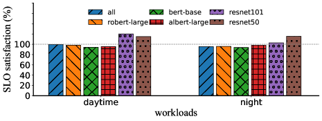
Figure 14 shows the throughputs required by SLOs and the throughputs provided by MIG-serving, for different services. In general, MIG-serving achieves $>$95% satisfaction rate for the required throughputs. The $<$5% difference is due to the slight performance variance between the model performance profiling (§2.2, Appendix B) and the performance of serving frameworks (e.g., Tensorflow-serving [36]). This can be improved by collecting model performance in production and gradually updating profiling data used in MIG-serving’s algorithms.

9 Related work

Scheduling problems. Scheduling problems [40] have been well-studied by multiple communities. the Reconfigurable Machine Scheduling Problem is an instance $(R_{m}|reconf|*)$ that captures DNNs and MIG’s characteristics: (a) model throughputs do not grow linearly with additional resources, (b) MIG-enabled GPUs follow specific reconfiguration rules, and (c) support partial reconfiguration.

The problem UPM [40] (Unrelated Parallel Machine Scheduling Problem) tackles (a), but it requires a fixed set of machines and does not capture MIG’s reconfigurability. Problems with RMTs [31] (Reconfigurable Machine Tools) address (b) and potentially (a). Examples are FJSSP-CDST [33] and permutation flow shop plus RMTs [16]. But they do not support partial reconfiguration because RMTs have fixed-sized reconfigurable units. The problem DCSP [23, 28] (Discrete-Continuous Scheduling Problem) supports (a) and (c), but the resources (in our case, GPU slices) have to be continuous (like power). But on the contrary, our problem has discrete resources and their allocation is restricted, as indicated by (b).

Partial reconfiguration. Similar to MIG-enabled GPUs, FPGA also supports partial reconfiguration [2]. A classic reconfigurable device model is the 2D resource model [45, 46] which abstracts a job with two constraints, width and height, representing the runtime and spatial constraints. The 2D model targets a similar but different problem: a job in the model has a fixed width and height, which in our context means that a service can use one fixed-sized GPU instance.

AmorphOS [29] is a system that manages and shares reconfigurable fabric (i.e., FPGA), and leverages FPGA partial reconfigurations. AmorphOS has multiple innovations. The one related to MIG-serving is AmorphOS’s scheduler which uses a two-mode approach (called low-latency mode and high-throughput mode) to schedule jobs based on the current workloads and FPGA status. In the context of the Reconfigurable Machine Scheduling Problem, this approach is a rule-based best-effort scheduling algorithm. Instead of being best-effort, MIG-serving’s algorithms consider wholistically and search in a large configuration space.

DNN serving systems. Traditional DNN serving systems—for example, Tensorflow-serving [36], TorchServe [1], Clipper [20]—mainly focus on optimizing the performance for a single service instance, whereas MIG-serving works on a layer below their abstraction: MIG-serving targets planning GPU instances hence is complementary to them; these serving frameworks can run within instances created by MIG-serving.

Another thread of DNN serving systems [22, 43, 25, 18, 42] aims at different workloads or specific DNN models. Though, conceptually, MIG-serving are complementary to these systems and can run beneath them, it requires further research to unleash the full potential of both systems. For example, BatchMaker [22] improves RNN’s inference performance by cellular batching. Similarly, Nexus [43] accelerates DNN serving by batching requests partially across different DNN models. Because the acceleration of these systems depends on how much portion of requests can be batched, serving performance varies with workloads. This is a challenge for MIG-serving as our algorithms require stable performance as inputs. Likewise, Clockwork [25] requires the full control over the execution stack to achieve predicable inference latency, whose scheduling decisions may conflict with MIG-serving controller’s.

DNN training scheduler. Scheduling DNN training, especially distributed training, has been intensively studied [47, 19, 24, 32, 37, 38, 49]. Though the Reconfigurable Machine Scheduling Problem covers the problem of DNN training scheduling, MIG-serving only tackles DNN serving. As stated in section 3.3, the problem of scheduling DNN inference services is simpler because DNN services are long-running. How to apply MIG-serving’s techniques to training is our future work.

Though having different contexts, some training systems use related techniques to MIG-serving. Gavel [35] encodes the problem of training DNNs on heterogeneous GPUs into an integer programming problem, and uses a solver to solve the problem. Likewise, MIG-serving’s problem can also be expressed in mixed integer programming. We’ve tried this, but our implementation (in Z3 [21]) does not meet our performance requirement—it solves a 5-GPU problem in 20min. Pollux [41] uses Genetic Algorithms (GA) to optimize cluster-wide “goodput” (a combination of training throughput and efficiency) by dynamically re-assigning resources to different jobs. MIG-serving also uses GA, but the similarity stops here; the two systems have different targets and the contents of GA operations are different.

Heuristic algorithms. Many real-world problems are NP-complete, and in practice people use heuristic algorithms to “solve” them. Our work MIG-serving shares the same spirit and is indebted to many prior algorithms and systems. For example, AlphaGo [44] inspires MIG-serving’s customized MCTS algorithm (§5.3). Similarly, SwapAdvisor [26] enlightens us to use the Genetic Algorithm in MIG-serving.

10 Summary and future work

This paper studies a new hardware feature, MIG, introduced by NVIDIA A100 GPUs. To capture the characteristics of MIG and DNN models running on it, we introduce a new abstract problem, the Reconfigurable Machine Scheduling Problem. Further, we design and implement a system, MIG-serving, which addresses the problem of serving DNN models with MIG. Evaluation shows that MIG-serving can save up to 40% GPUs versus using A100 as a whole.

MIG is a new hardware feature, and there are many future works to explore, just name a few: first, MIG-serving only focuses on serving. How to apply MIG-serving’s techniques to training is our future work. Second, MIG-serving’s current slow algorithm—MCTS—needs improvement (§11). We plan to fine-tune MCTS, or replace MCTS with other heuristic algorithms, or use (SMT or MIP) solvers to improve the slow algorithm. Third, the Reconfigurable Machine Scheduling Problem (RMS) is a new abstract problem, which has the potential to extend to other reconfigurable devices, such as FPGA. One of our future work is to comprehensively study what devices can be abstracted by the RMS and how would our algorithms help in those scenarios.

Appendix A MIG-serving algorithms

A.1 Heuristic greedy algorithm

As mentioned in section 5.3, MIG-serving uses a greedy algorithm as the fast algorithm which is based on a heuristic score. Figure 15 describes this greedy algorithm in detail.

In section 5.3, we deliberately omitted some technicalities for simplicity. Specifically, in order to keep the each round of search manageable, the algorithm only consider mixing two services in one GPU (Line 2, Figure 15). But, when all services are about to be fully satisfied, the algorithm changes its behavior by mixing more services in one GPU (Line 20, Figure 15). This is because two services can no longer saturate a GPU, and the algorithm needs to pack more services.

A.2 Customized MCTS

As stated in section 5.3, vanilla MCTS does not work for our problem because of two challenges: (i) tree node has too many children and (ii) the classic MCTS estimation procedure is slow and inaccurate. We elaborate how MIG-serving addresses these two challenges below.

For the first challenge, MIG-serving cuts the space by only having the configurations with top-K scores for a node. Specifically, for each node (i.e., completion rates), MIG-serving randomly picks five services which are not fully satisfied and calculates scores (§5.3) for the GPU configurations having these services. Then MIG-serving chooses the top-K configurations (K=10 by default) as edges to this node and generates the corresponding child nodes.

For the second challenge, MIG-serving develops a fast and accurate estimation by memoization and randomization. In particular, MIG-serving’s estimation pre-calculates and caches some good candidates for different types of completion rates. During the estimation procedure, MIG-serving maps the current node to a type of completion rates (roughly), and randomly chooses a child node from the pool of good candidates. It repeats this step until reaches some leaf node. Our experiments show that this estimation approach is about two to three orders of magnitude faster than the classic estimation and is accurate.

1:procedure FastAlgo(comp_rates)

2:    $\textit{conf\_set}\leftarrow$ all GPU configs mixing at most 2 services

3:    $\textit{ret}\leftarrow$ empty list

4:    while True:

5:        $\textit{max\_score}\leftarrow 0$

6:        $\textit{best\_conf}\leftarrow\textit{None}$

7:        

8:        for $\textit{conf}\in\textit{conf\_set}$:     // find the best config

9:            $\textit{score}\leftarrow$ calculate score for conf    //§5.3

10:            if $\textit{score}>\textit{max\_score}$:

11:               max_score$\leftarrow$ score

12:               best_conf$\leftarrow$ conf                     

13:        

14:        $\textit{ret}+=\textit{best\_conf}$

15:        update comp_rates according to best_conf’s utility

16:        if $\textit{comp\_rates}>=[100\%]*len(\textit{comp\_rates})$:

17:            return ret         

18:        

19:        for $\textrm{service}_{i}$ in all services:

20:            if $\textrm{service}_{i}$ is almost satisfied:

21:               confs $\leftarrow$ mixing $\textrm{service}_{i}$ with more services

22:               $\textit{conf\_set}+=\textit{confs}$                         

Figure 15: MIG-serving’s fast algorithm (§5.3).

Appendix B A study of serving performance with MIG

As mentioned in section 2.2, to understand inference performance on different sized instances, we experiment with 49 open sourced models in PyTorch Hub [14] and TensorFlow Hub [15], and collect model inference throughputs and latencies. This section describes the experiment details and provides results from more models than the two in section 2.2.

Experimental setup. Our testbed is a machine with AMD EPYC 7742 CPU with 64 cores, 1.96 TB memory, running Debian 9 (stretch) OS, CUDA 11.0.207, NVIDIA driver version 450.80.02.

In our experiments, we do not use the serving frameworks like TensorFlow serving or TorchServe because we want to evaluate inference throughputs and latencies of GPUs only, without queueing effects or the overheads from these serving frameworks. Therefore, we develop our own benchmarking tool which prepares the inputs in memory and directly call models’ inference functions. The latencies collected by the tool are the running time of model inference on GPUs, which do not include overheads from inter-process communication or network costs.

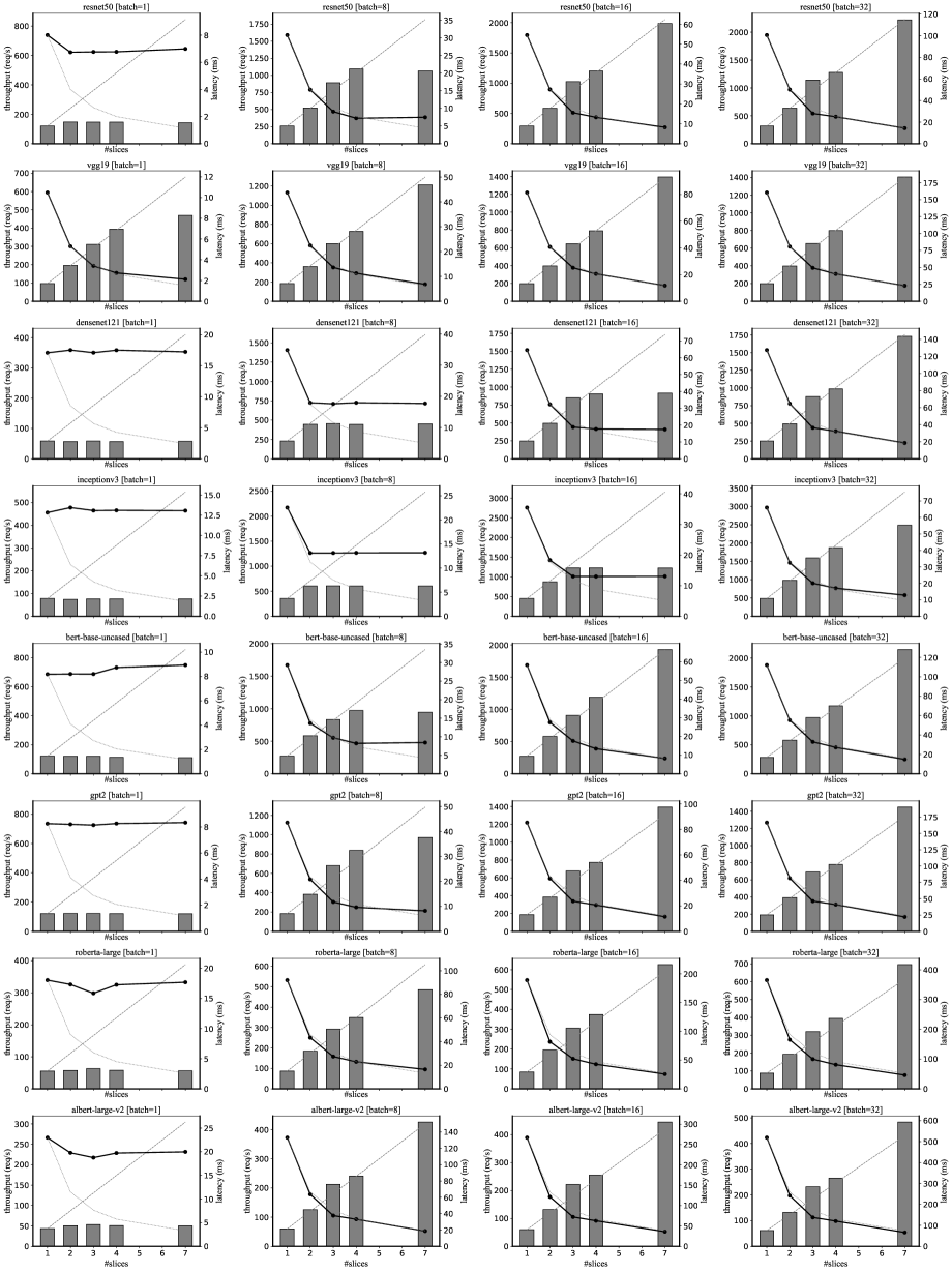
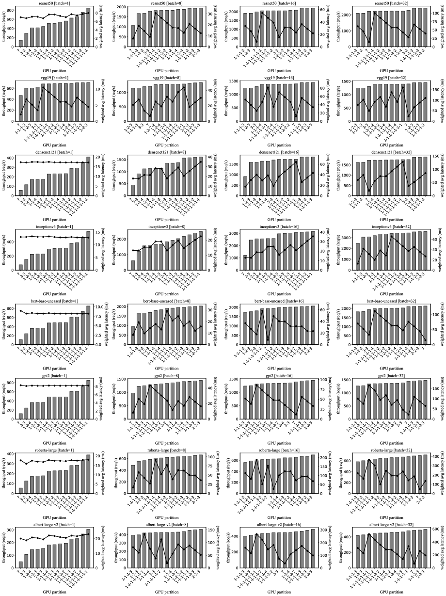
PyTorch. We run PyTorch 1.9.0. Models are fetched from Pytorch Hub. Figure 16 shows the single instance throughputs and latencies for 8 models that exist in both PyTorch’s and TensorFlow’s model hub (resnet50, vgg19, densenet121, inceptionv3, bert-base-uncased, gpt2, roberta-large, and albert-large-v2) of four batch sizes (1, 8, 16, 32). Figure 17 shows the throughputs and latencies for different GPU partitions of the same 8 models.

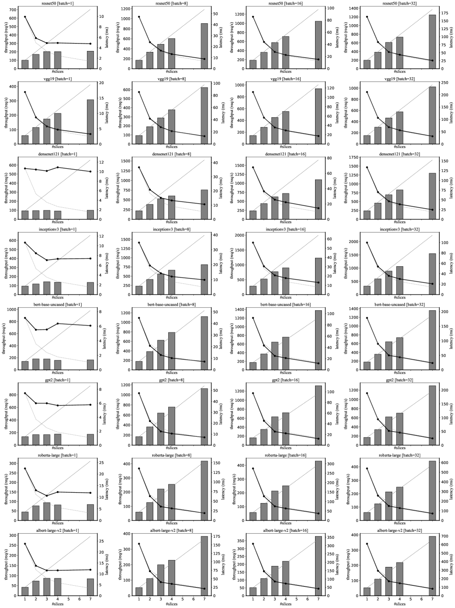
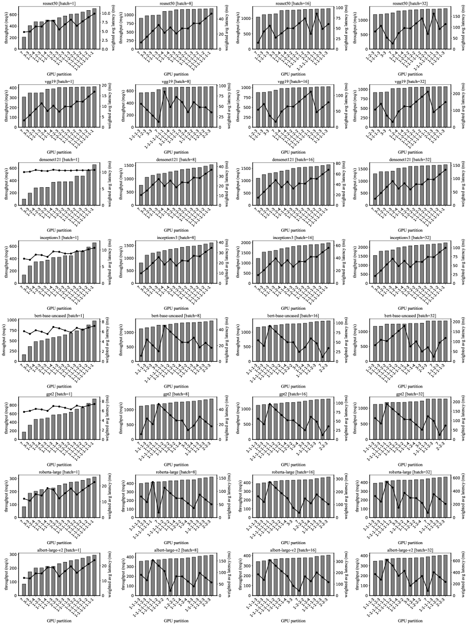
TensorFlow. We run TensorFlow 2.4.1. Models are fetched from tensorflow.keras.applications module and transformers 4.5.1 which is a popular Python library for natural language processing. Figure 18 shows the single instance throughputs and latencies for the same 8 models as PyTorch’s above and in four batch sizes (1, 8, 16, 32). Figure 19 shows the throughputs and latencies for different GPU partitions of the same 8 models.

Figure 16: PyTorch model inference throughputs and latencies for 1/7–7/7 instances.

Figure 17: PyTorch model inference throughputs and latencies for distinct GPU partitions.

Figure 18: TensorFlow model inference throughputs and latencies for 1/7–7/7 instances.

Figure 19: TensorFlow model inference throughputs and latencies for distinct GPU partitions.

References

- [1] TorchServe. https://pytorch.org/serve/.
- [2] Vivado Design Suite User Guide Partial Reconfiguration. https://www.xilinx.com/support/documentation/sw_manuals/xilinx2018_1/ug909-vivado-partial-reconfiguration.pdf, 2018.
- [3] Amazon EC2 G4 Instances. https://aws.amazon.com/ec2/instance-types/g4/, 2021.
- [4] Amazon EC2 P3 Instances. https://aws.amazon.com/ec2/instance-types/p3/, 2021.
- [5] Amazon EC2 P4d Instances. https://aws.amazon.com/ec2/instance-types/p4/, 2021.
- [6] Cutting stock problem. https://en.wikipedia.org/wiki/Cutting_stock_problem, 2021.
- [7] GPU cloud computing solution. https://www.nvidia.com/en-us/data-center/gpu-cloud-computing/, 2021.
- [8] Kubernetes Controllers. https://kubernetes.io/docs/concepts/architecture/controller/, 2021.
- [9] Minimizing Deep Learning Inference Latency with NVIDIA Multi-Instance GPU. https://developer.nvidia.com/blog/minimizing-dl-inference-latency-with-mig/, 2021.
- [10] NVIDIA A100. https://www.nvidia.com/en-us/data-center/a100/, 2021.
- [11] NVIDIA A100 Tensor Core GPU Architecture. https://www.nvidia.com/content/dam/en-zz/Solutions/Data-Center/nvidia-ampere-architecture-whitepaper.pdf, 2021.
- [12] NVIDIA Data Center Deep Learning Product Performance. https://developer.nvidia.com/deep-learning-performance-training-inference, 2021.
- [13] NVIDIA Multi-Instance GPU User Guide. https://docs.nvidia.com/datacenter/tesla/pdf/NVIDIA_MIG_User_Guide.pdf, 2021.
- [14] PyTorch Hub. https://pytorch.org/hub/, 2021.
- [15] TensorFlow Hub. https://tfhub.dev/, 2021.
- [16] A. Azab and B. Naderi. Modelling the problem of production scheduling for reconfigurable manufacturing systems. Procedia CIRP, 33:76–80, 2015.
- [17] Z. Bai, Z. Zhang, Y. Zhu, and X. Jin. Pipeswitch: Fast pipelined context switching for deep learning applications. In 14th USENIX Symposium on Operating Systems Design and Implementation (OSDI 20), 2020.
- [18] A. Balasubramanian, A. Kumar, Y. Liu, H. Cao, S. Venkataraman, and A. Akella. Accelerating deep learning inference via learned caches. arXiv preprint arXiv:2101.07344, 2021.
- [19] S. Chaudhary, R. Ramjee, M. Sivathanu, N. Kwatra, and S. Viswanatha. Balancing efficiency and fairness in heterogeneous gpu clusters for deep learning. In Proceedings of the Fifteenth European Conference on Computer Systems, 2020.
- [20] D. Crankshaw, X. Wang, G. Zhou, M. J. Franklin, J. E. Gonzalez, and I. Stoica. Clipper: A low-latency online prediction serving system. In 14th USENIX Symposium on Networked Systems Design and Implementation (NSDI 17), 2017.
- [21] L. De Moura and N. Bjørner. Z3: An efficient smt solver. In International conference on Tools and Algorithms for the Construction and Analysis of Systems, pages 337–340. Springer, 2008.
- [22] P. Gao, L. Yu, Y. Wu, and J. Li. Low latency rnn inference with cellular batching. In Proceedings of the Thirteenth EuroSys Conference, 2018.
- [23] M. Gorczyca, A. Janiak, and W. Janiak. The discrete part of the discrete-continuous scheduling problems-new properties. IFAC Proceedings Volumes, 42(13):244–249, 2009.
- [24] J. Gu, M. Chowdhury, K. G. Shin, Y. Zhu, M. Jeon, J. Qian, H. Liu, and C. Guo. Tiresias: A GPU cluster manager for distributed deep learning. In 16th USENIX Symposium on Networked Systems Design and Implementation (NSDI 19), pages 485–500, 2019.
- [25] A. Gujarati, R. Karimi, S. Alzayat, W. Hao, A. Kaufmann, Y. Vigfusson, and J. Mace. Serving dnns like clockwork: Performance predictability from the bottom up. In 14th USENIX Symposium on Operating Systems Design and Implementation (OSDI 20), 2020.
- [26] C.-C. Huang, G. Jin, and J. Li. Swapadvisor: Pushing deep learning beyond the gpu memory limit via smart swapping. In Proceedings of the Twenty-Fifth International Conference on Architectural Support for Programming Languages and Operating Systems, pages 1341–1355, 2020.
- [27] K. Jansen, A. Lassota, and M. Maack. Approximation algorithms for scheduling with class constraints. In Proceedings of the 32nd ACM Symposium on Parallelism in Algorithms and Architectures, pages 349–357, 2020.
- [28] J. Józefowska, M. Mika, R. Różycki, G. Waligóra, and J. Węglarz. Solving discrete-continuous scheduling problems by tabu search. In 4th Metaheuristics International Conference MIC, pages 16–20, 2001.
- [29] A. Khawaja, J. Landgraf, R. Prakash, M. Wei, E. Schkufza, and C. J. Rossbach. Sharing, protection, and compatibility for reconfigurable fabric with amorphos. In 13th USENIX Symposium on Operating Systems Design and Implementation (OSDI 18), pages 107–127, 2018.
- [30] D.-W. Kim, K.-H. Kim, W. Jang, and F. F. Chen. Unrelated parallel machine scheduling with setup times using simulated annealing. Robotics and Computer-Integrated Manufacturing, 18(3-4):223–231, 2002.
- [31] R. G. Landers, B.-K. Min, and Y. Koren. Reconfigurable machine tools. CIRP Annals, 50(1):269–274, 2001.
- [32] K. Mahajan, A. Balasubramanian, A. Singhvi, S. Venkataraman, A. Akella, A. Phanishayee, and S. Chawla. Themis: Fair and efficient GPU cluster scheduling. In 17th USENIX Symposium on Networked Systems Design and Implementation (NSDI 20), 2020.
- [33] M. Mahmoodjanloo, R. Tavakkoli-Moghaddam, A. Baboli, and A. Bozorgi-Amiri. Flexible job shop scheduling problem with reconfigurable machine tools: An improved differential evolution algorithm. Applied Soft Computing, 94:106416, 2020.
- [34] L. Min and W. Cheng. A genetic algorithm for minimizing the makespan in the case of scheduling identical parallel machines. Artificial Intelligence in Engineering, 13(4):399–403, 1999.
- [35] D. Narayanan, K. Santhanam, F. Kazhamiaka, A. Phanishayee, and M. Zaharia. Heterogeneity-aware cluster scheduling policies for deep learning workloads. In 14th USENIX Symposium on Operating Systems Design and Implementation (OSDI 20), pages 481–498, 2020.
- [36] C. Olston, N. Fiedel, K. Gorovoy, J. Harmsen, L. Lao, F. Li, V. Rajashekhar, S. Ramesh, and J. Soyke. Tensorflow-serving: Flexible, high-performance ml serving. arXiv preprint arXiv:1712.06139, 2017.
- [37] Y. Peng, Y. Bao, Y. Chen, C. Wu, and C. Guo. Optimus: an efficient dynamic resource scheduler for deep learning clusters. In Proceedings of the Thirteenth EuroSys Conference, pages 1–14, 2018.
- [38] Y. Peng, Y. Zhu, Y. Chen, Y. Bao, B. Yi, C. Lan, C. Wu, and C. Guo. A generic communication scheduler for distributed dnn training acceleration. In Proceedings of the 27th ACM Symposium on Operating Systems Principles, pages 16–29, 2019.
- [39] F. Pezzella, G. Morganti, and G. Ciaschetti. A genetic algorithm for the flexible job-shop scheduling problem. Computers & Operations Research, 35(10):3202–3212, 2008.
- [40] M. Pinedo. Scheduling, volume 29. Springer, 2012.
- [41] A. Qiao, W. Neiswanger, Q. Ho, H. Zhang, G. R. Ganger, and E. P. Xing. Pollux: Co-adaptive cluster scheduling for goodput-optimized deep learning. arXiv preprint arXiv:2008.12260, 2020.
- [42] F. Romero, Q. Li, N. J. Yadwadkar, and C. Kozyrakis. Infaas: A model-less inference serving system. arXiv preprint arXiv:1905.13348, 2019.
- [43] H. Shen, L. Chen, Y. Jin, L. Zhao, B. Kong, M. Philipose, A. Krishnamurthy, and R. Sundaram. Nexus: a gpu cluster engine for accelerating dnn-based video analysis. In Proceedings of the 27th ACM Symposium on Operating Systems Principles, 2019.
- [44] D. Silver, J. Schrittwieser, K. Simonyan, I. Antonoglou, A. Huang, A. Guez, T. Hubert, L. Baker, M. Lai, A. Bolton, et al. Mastering the game of go without human knowledge. nature, 550(7676):354–359, 2017.
- [45] C. Steiger, H. Walder, and M. Platzner. Operating systems for reconfigurable embedded platforms: Online scheduling of real-time tasks. IEEE Transactions on computers, 53(11):1393–1407, 2004.
- [46] Z. Wang, Q. Tang, B. Guo, J.-B. Wei, and L. Wang. Resource partitioning and application scheduling with module merging on dynamically and partially reconfigurable fpgas. Electronics, 9(9):1461, 2020.
- [47] W. Xiao, R. Bhardwaj, R. Ramjee, M. Sivathanu, N. Kwatra, Z. Han, P. Patel, X. Peng, H. Zhao, Q. Zhang, et al. Gandiva: Introspective cluster scheduling for deep learning. In 13th USENIX Symposium on Operating Systems Design and Implementation (OSDI 18), 2018.
- [48] W. Xing and J. Zhang. Parallel machine scheduling with splitting jobs. Discrete Applied Mathematics, 103(1-3):259–269, 2000.
- [49] H. Zhao, Z. Han, Z. Yang, Q. Zhang, F. Yang, L. Zhou, M. Yang, F. C. Lau, Y. Wang, Y. Xiong, et al. Hived: Sharing a GPU cluster for deep learning with guarantees. In 14th USENIX Symposium on Operating Systems Design and Implementation (OSDI 20), pages 515–532, 2020.
Appendix A \xmakefirstucMIG-serving algorithms