Chaos in self-gravitating many-body systems

In self-gravitating $N$-body systems, small perturbations introduced at the start, or infinitesimal errors that are produced by the numerical integrator or are due to limited precision in the computer, grow exponentially with time. For Newton’s gravity, we confirm earlier results that for relatively homogeneous systems, this rate of growth per crossing time increases with $N$ up to $N\sim 30$, but that for larger systems, the growth rate has a weaker scaling with $N$. For concentrated systems, however, the rate of exponential growth continues to scale with $N$. In relativistic self-gravitating systems, the rate of growth is almost independent of $N$. This effect, however, is only noticeable when the system’s mean velocity approaches the speed of light to within three orders of magnitude. The chaotic behavior of systems with more than a dozen bodies for the usually adopted approximation of only solving the pairwise interactions in the Einstein-Infeld-Hoffmann equation of motion is qualitatively different than when the interaction terms (or cross terms) are taken into account. This result provides a strong motivation for follow-up studies on the microscopic effect of general relativity on orbital chaos, and on the influence of higher-order cross-terms in the Taylor-series expansion of the Einstein-Infeld-Hoffmann equations of motion.

1 Introduction

Soon after the first gravitational $N$-body problems were computed (von Hoerner 1960; Aarseth & Hoyle 1964; van Albada 1968), Miller (1964) questioned the validity of such simulations. The nature of his concern was based on the intrinsically chaotic behavior of Newton’s law of gravity. Errors during integration are introduced by the limited precision of the computer, together with the limited accuracy of the numerical integration scheme. The exponential growth of both sources of errors then contributes to the lack of reproducibility in $N$-body simulations (Boekholt et al. 2020).

In an attempt to acquire a converged solution to the 25-body problem, Hayli (1970) integrated Newton’s equations of motion using various precisions on a 60 bit CDC 6400, a 64 bit IBM 360/365, and an 80 bit Honeywell-Bull CII 90–80. He found that although identical initial realizations were used, he acquired a different answer for the final positions and velocities of the 25 objects in his calculations, even with the same algorithm and time step. He argued that the difference in precision of the floating-point unit was responsible for the lack of reproducibility of the results. Because the IEEE standard for floating-point arithmetic (IEEE 754) was only introduced in 1985, the discrepancy identified by Hayli (1970) could also have originated from differences in round-off in the least significant digit of the various machines. We still encounter this problem in today’s Graphical Processing Units (GPU), which have limited precision (Fortin et al. 2012). These sources of errors, time step, and round-off make individual solutions to the $N$-body problem notoriously unreliable, although statistically, they may still have the correct phase-space distribution characteristics (Boekholt & Portegies Zwart 2015; Hernandez et al. 2020). The common agreement on round-off among computer manufacturers, compiler designers, and operating systems hides this problem by generating identical output when the same initial realization is run using different hardware and operating systems, so long as the same source code is run on a single core, and compilers are not too different.

It is a common assumption among $N$-body practitioners that the microscopic unpredictability and the consequential loss of reproducibility is irrelevant so long as the global phase-space characteristics are still representative of true physics. It remains an article of faith that such a statistical validity holds for the Newtonian N-body problem (Heggie 1991). Chaos, however, leads to unpredictability due to temporal discretization, round-off, and uncertainty in the initial realization (Miller 1964). Unpredictability due to chaotic behavior and the consequential loss of reproducibility may then lead to incorrect physical results.

After the pioneering work of Hayli (1970), the problem of characterizing chaos in self-gravitating $N$-body systems received little attention until the late 1980s (except possibly in Zadunaisky 1979, in which the focus was on the computer’s precision), when computers became sufficiently powerful to address the problem for larger $N$ (Heggie 1988; Kandrup & Smith 1991, 1992; Kandrup et al. 1992; Goodman et al. 1993; Gurzadyan & Kocharyan 1994; Kandrup et al. 1994; Fukushige & Makino 1994). Goodman et al. (1993) and Fukushige & Makino (1994) provided excellent overviews of the underlying arguments for this chaotic behavior in few- and many-body systems, respectively.

Even today, the chaotic $N$-body problem is hard to address adequately using digital computers, and there is still no analytic solution. We address three aspects of the problem here: 1) the veracity of a solution for $N=4$ to $1024$, 2) the scaling of the growth of errors to large $N\ga 10^{5}$, and 3) the effect of general relativity on the chaotic behavior of $N$-body systems. The terminology used in this text is explained in the glossary in Portegies Zwart & Boekholt (2018). Loosely speaking, a reprehensive solution is a solution in which the errors introduced during integration exceed the system size. For a veracious solution, this is not the case. For $N=3$, Boekholt & Portegies Zwart (2015) demonstrated that veracious $N$-body solutions give statistically indistinguishable results as an ensemble of converged solutions. They called this behavior Nagh Hoch, to signify the importance of consistent statistical ensemble average behavior of veracious solutions to the chaotic self-gravitating $N$-body problem. It is not clear if this concept also holds for larger $N$.

Hernandez et al. (2020) studied Nagh Hoch by running ensembles of reprehensible numerical solutions for planetary systems. They integrated a single $3\cdot 10^{-5}$ mass planet in a circular orbit at a distance of 0.29 (in dimensionless $N$-body units, Hénon 1971) from the star, together with a test particle in the same plane at apocenter and with an eccentricity of 0.19 and semimajor axis 0.21. The calculations were conducted for 200 $e$-foling timescales using four different algorithms for solving the equations of motion. They found that for a sufficiently large sample of initial realizations and a tolerably small time step, the results of the various integrators are statistically indistinguishable. We conclude from their simulation results that their adopted reprehensive N-body algorithms for a system of two planets complies to Nagh Hoch. They argue that a relative integration error $\la 0.05$ is sufficient to preserve the quality, consistent with Boekholt & Portegies Zwart (2015), who argued that a time step smaller than $2^{-5}$ is sufficient to preserve ergodicity in the outcome space.

Ideally, one would like to perform large $N$-body simulations to a converged solution, but this is unrealistic, even on modern digital computers. We can achieve converged solutions for $N$ up to about $1$k particles for several crossing times, leading to a series of veracious solutions. At the moment, however, a longer evolution or a larger number of particles are too costly. However, we demonstrate that the chaotic behavior of these systems is reprehensive and confirm that they show statistically indistinguishable chaotic behavior. We subsequently perform reprehensible $N$-body simulations for up to $128$k particles.

The interest in scaling to $N\gg 3$ is in part motivated by understanding the chaotic nature of galaxies. Dense stellar systems, such as globular clusters [$N={\cal O}(10^{6})$], are highly chaotic (Parvulesco 1924; Carpintero et al. 1999). Galaxies ($N\rightarrow\infty$) are considered collisionless because their relaxation time exceeds the Hubble time (Binney & Tremaine 2008). For sufficiently large $N$ the background potential becomes smooth, and the collisionless assumption becomes increasingly applicable (Muzzio & Mosquera 2004; Muzzio et al. 2009). However, due to the point-particle granularity of the potential, the microscopic exponential instability remains present in the system (Valluri & Merritt 2000). Even large $N$-systems are therefore affected by the chaos in small-$N$ subsystems. It is nonetheless unclear how the microscopic exponential instability propagates to the macroscopic structure of the stellar system as a whole. At which value of $N$ does the system exhibit the transition from chaotic small-$N$ to smooth large-$N$ systems?

Heggie (1988) argued that the dynamics $N$-body systems under Newton’s equations of motion are dominated by encounters at an impact parameter of about $r/N^{1/2}$. Since chaos is driven by encounters, the Lyapunov timescale then has a similar scaling. In a pioneering study, Goodman et al. (1993) discussed this scaling and found a transition in the chaotic behavior around $N\simeq 32$. They argued that the Lyapunov timescale is proportional to the dynamical crossing time $t_{\lambda}\propto\gamma t_{cr}/\ln(\ln(N))$ over all values of $N$. For large $N$ ($\ga 32$), the constant $\gamma$ is smaller, leading to a weaker dependence on the Lyapunov timescale (see also Kandrup & Smith 1992; Kandrup 1998). Hemsendorf & Merritt (2002) found a similar transition, but argued in favor of scaling $t_{\lambda}\propto 1/\ln(N)$ over the entire range of $N$. In this latter study, however, the perturbed particle is evolved in a static background (Hemsendorf & Merritt 2002), and it is not clear if their different scaling resulted from this particular assumption or from the slightly different potential. We therefore extend the range for which the Lyapunov time was determined to $N=128$k using reprehensive $N$-body solutions, allowing us to test the scaling of the Lyapunov timescale to large $N$ in an actual self-gravitating system. In addition, we chose various initial density profiles: a smooth profile (as in Goodman et al. (1993)), a Plummer profile (1911, as in Hemsendorf & Merritt 2002) , and a King profile ($W_{o}=12$, King 1966, just for fun).

The change in slope near $N\simeq 32$ pinpoints the transition from chaotic behavior driven by local few-body relaxation (for $N\la 32$) to far-field many-body relaxation. This transition can globally be understood by comparing the dynamical crossing time $t_{\rm cross}$ with the two-body relaxation time $t_{\rm rlx}$  , which can be approximated by (Spitzer 1971; Spitzer & Hart 1971b, a; Spitzer 1987)

$$t_{\rm rlx}\simeq\left({N\over 8\ln(N)}\right)t_{\rm cross}.$$ (1)

This relation indicates that for $N\ga 32$, the relaxation timescale exceeds the crossing time. It remains unclear, however, which underlying process determines the slope.

Hemsendorf & Merritt (2002) argued in favor of the same scaling for all $N$ and suggested that a galaxy with $10^{12}$ stars would have a Lyapunov timescale of $t_{\lambda}\approx t_{cr}/30$ or $t_{\lambda}\sim 8$ Myr, whereas Goodman et al. (1993) argued for a Lyapunov timescale that is roughly an order of magnitude larger. Regardless of either of the two scaling relations, the Galaxy would be subject to chaotic motion on a fraction of the crossing timescale, and would therefore not be representable by the collisionless Boltzmann equation (Boltzmann 1872).

For the Solar System, there seems to be a difference as well, this time, in terms of chaotic behavior. In the Newtonian case, resonances between Jupiter and Mercury greatly enhance the eccentricity of the orbit of the latter planet. This may eventually lead to a collision between Mercury and the Sun (Laskar et al. 1992; Milani & Nobili 1992). However, the inclusion of relativistic effect tends to stabilize the system, resulting in the much-reduced probability that Mercury collides with the Sun (Laskar & Gastineau 2009). Based on our results, we tend to agree with the increased stability of the Solar System when considering relativistic mechanics. Interestingly, the global Lyapunov timescale for the Solar System is not dissimilar from the galactic result, being $\sim 5$ Myr (Laskar et al. 1992) to $\ga 6.8$ Myr (Applegate et al. 1986) or even slightly longer (Duncan & Quinn 1993; Batygin et al. 2015).

We argue that ensembles of reprehensive $N$-body solutions, from $N=4$ to $1024$ ($1k$), give statistically the same chaotic behavior as the converged solutions. This trend holds at least up to $N=1k$, for which we acquire converged solutions for $10$ Hénon time units (equivalent to four crossing times). It becomes rather unpractical to continue with converged solutions for $N\geq 1k$.

Regardless of the large-$N$ behavior of the chaotic self-gravitating systems under Newton’s forces, we also study the relativistic case. Rather than solving Einstein’s field equations directly, we address relativistic dynamics through an expansion to the gravitational field in terms of $v/c$, which expresses the speed of light ($c$) in dimensionless $N$-body units in terms of the velocity of the particles ($v$). The zeroth order in this expansion represents Newton’s equations of motion, which does not depend on the velocity. The first-order post-Newtonian term (the 1-PN) is proportional to $v^{2}/c^{2}$, describes the motion of $N$ Schwarzschild black holes, and is known as the Einstein-Infeld-Hoffmann (EIH) equation (Einstein et al. 1938). Lorentz & Droste (1917) worked out a first generalization for these post-Newtonian $N$-body equations of motion, but the final formulation was realized by Einstein et al. (1938).

Our study is motivated by the generally adopted view that the radiation-induced dissipation in general relativity quenches the chaotic behavior of the $N$-body system. Spyrou (1975, but see also, Wanex 2002; Cornish & Levin 2003; Galaviz 2011; Neilsen et al. 2014) demonstrated that the pairwise post-Newtonian expansion to 2.5th order is chaotic in democratic three-body systems. They also studied the gravitational-wave signal for such systems (Gültekin et al. 2006). Chaotic behavior was not demonstrated for relativistic systems with more than three particles.

We adopt the EIH equation and compare the degree of chaos measured in systems from $N=3$ to $N=1k$ with the Newtonian solutions ($v/c\rightarrow 0$). Our approach, however, is limited to first-order post-Newtonian correction terms for the EIH equations of motion. The 1-PN terms are not dissipative and therefore are not expected to result in less chaotic behavior when compared to Newton’s equations of motion.

The motivation for performing our a study is somewhat academic because it is currently unclear to which degree large-$N$ relativistic systems appear in nature or how frequently they emit gravitational waves in an observable wavelength. Galactic nuclei are probably the most promising places to find multiple supermassive black holes orbited by intermediate-mass black holes or other compact objects. Portegies Zwart et al. (2006) argued that the Galactic center would be populated by a steady population of a dozen intermediate-mass black holes within a few milliparsec of the supermassive black hole. In addition, there could be many stellar-mass black holes and a rich population of neutron stars in the Galactic center (Muno et al. 2004; Rimoldi et al. 2015). These black holes may merge, producing observable gravitational-wave signals (Pretorius 2005; Abbott et al. 2017) and high-velocity recoiling black holes (Campanelli et al. 2007). Similar, but less extreme, situations may be present in the cores of some globular clusters (Banerjee et al. 2010; Banerjee 2021). Banerjee & Kroupa (2011) even speculated that clusters composed only of dark objects might exist, which could be copious sources of gravitational radiation. Recently, Gieles et al. (2021) argued that the globular cluster Palomar 5 may host such a central collection of compact objects and that in the coming 100 Myr, its entire core may be composed of black holes. With the current rather large virial radius, the dynamics in this cluster is not expected to be subject to strong relativistic effects, however.

It would be interesting to determine the gravitational-wave signature of such chaotic systems and maybe even search for them in the data collected by gravitational-wave observatories. An analysis like this was done for hierarchical triples (Galaviz & Brügmann 2011; Meiron et al. 2017; Robson et al. 2018; Lim & Rodriguez 2020; Will 2021), but not for $N>3$.

2 Methods

In the gravitational many-body problem, $N$ objects move under the attractive influence and space-time distortions of each other. We use three independently developed implementations of the force-law and integration method. One of these is the code ph4  (see Appendix A, McMillan 2014), which is designed for the problem of $N$ point masses under a Newtonian force law with regular hardware and compiler-supported precision (see sec. 2.1) For chaotic systems, one may desire more control over the precision and accuracy of the integrator because reprehensible $N$-body calculations provide insufficient trust due to round-off and integration errors that grow exponentially with time. On the other hand, veracious calculations are also reprehensible, but are statistically indistinguishable from the converged solutions (Boekholt & Portegies Zwart 2015). We therefore also perform calculations using Brutus  (Portegies Zwart & Boekholt 2014), which allows us to control these parameters with a tolerance $\epsilon$ and word-length $L_{w}$ (see 2.2).

The relativistic calculations are performed up to the first post-Newton order using the pairwise approximation and the full EIH equations of motion. The relativistic $N$-body code is called Hermite_GRX,  and it is described in sect 2.3. The equations of motion in ph4  and Hermite_GRX  are integrated using the Hermite algorithm (Makino 1991) or an adaptation of it to accommodate the velocity dependence of the acceleration. In Brutus,  the equations of motion are solved with a second-order Verlet (1967) scheme.

We finally use these three methods to study chaos in the large-$N$ limit. Large here means $\sim 1$k for the post-Newton case and converged Newton solutions, and up to $N=128$k for reprehensible Newtonian solutions. Each of the codes is interfaced as a community code to the Astronomical Multipurpose Software Environment (Portegies Zwart & McMillan 2018). We describe these implementations in Appendix A.3.3.

2.1 Regular $N$-body calculations

According to Newton’s laws of motion, the acceleration $\@vec{a}_{i}$ on particle $i$ is given by the sum over all other particles (Newton 1687):

$$\@vec{a}_{i}=-\sum_{\begin{subarray}{c}j=1\\ j\neq i\end{subarray}}^{n}{Gm_{j}\over r_{ij}^{3}}\@vec{r}_{ij}.$$ (2)

Here $m_{i}$ is the mass of particle $i$, and $\@vec{r}_{ij}$ is the relative position vector from particle $i$ to $j$: $\@vec{r}_{ij}\equiv\@vec{r}_{i}-\@vec{r}_{j}$. Newton’s constant is $G={\cal O}(10^{-10}$ N/kg²/m²), but in our calculations, $G\equiv 1$ (Hénon 1971; Heggie & Mathieu 1986).

Integration was performed in 64-bits using IEEE 754 Standard for floating-point arithmetic under the Linux operating system with kernel version 5.8.0-48-generic. CPU calculations were performed on an 192 core Intel Xeon E7-8890 v4 workstation running at 2.20 GHz. Parallelization was realized using the Message Passing Interface (version Open MPI 4.0.3) (Portegies Zwart et al. 2008). For simulations with $N>1$k we adopted the GPU version of ph4, which uses the Sapporo  GPU library (Portegies Zwart et al. 2007; Gaburov et al. 2009) running on Xeon E-2176M CPU with Quadro P2000 Max-Q GPU. The GPU has $4$ GB GDDR5 RAM, but is not equipped with error correction, potentially leading to non-IEEE compliant errors in the calculations.

2.2 Arbitrarily precise $N$-body calculations

The Hermite algorithm is a fourth-order scheme that reaches a relative energy error $dE/E\simeq 10^{-15}$ with a time-step parameter $\eta\simeq 10^{-4}$ for a distribution of equal-mass objects in a virialized homogeneous distribution in space. All our calculations were performed with $\eta=0.01$. Round-off and time-step errors become important for smaller time steps when integrating for more than $\sim 10$ crossing times, resulting in a systematic growth of the energy error. This growth scales $\propto\eta^{2}$. Although small, typically about $1/10^{16}$ (in relative coordinates), these errors drive the eventual irreproducibility of the simulations through exponential growth. This irreproducibility is undesirable when one is interested in studying chaotic motion. We therefore also performed calculations with Brutus  (Boekholt & Portegies Zwart 2015), an $N$-body code that allows us to integrate any $N$-body system to arbitrary precision. In Brutus  we control the different sources of error by adopting the Gragg-Bulirsch–Stoer algorithm (Bulirsch & Stoer 1964; Gragg 1965). In this algorithm, one performs a single step using a Verlet integrator (Verlet 1967), then repeats that same step using half the step size. Now the relative error between the two solutions can be determined by taking the absolute value of the differences in each coordinate. If this error is smaller than some predetermined tolerance, the result is accepted, and the next step is calculated. Otherwise, the same step is repeated with a quarter time step. This procedure is repeated until the relative error between two subsequent solutions is smaller than the tolerance (see Press et al. 1992).

We controlled the discretization error with arbitrary-precision arithmetic, using the GMP (Granlund & the GMP development team 2012; Granlund & Team 2015) and MPFR libraries (Fousse et al. 2007) instead of conventional double precision. This allowed us to control the round-off error by changing the number of digits, which we express in a word-length $L_{w}$. A word-length $L_{w}=64$ bits then corresponds approximately to the usual 16-decimal place precision in standard IEEE 754 floating-point operations on current regular microprocessors.

In practice, we only specified the tolerance and calculated the word length $L_{w}\in\mathbb{Z}$ with (Boekholt & Portegies Zwart 2015),

$$L_{w}=\textrm{int}(32-4\log_{10}(\epsilon)).$$ (3)

A converged solution to $n$ decimal places is achieved by iteratively repeating a calculation that started with one selected realization of the initial conditions with lower tolerance for each subsequent calculation. This process is repeated until the first $n$ decimal places of the final phase-space coordinates of two subsequent iterations lead to identical values for the first $n$ digits in the positions and velocities of all particles. When the numerical solution has achieved this state of convergence, it is deemed to be definitive (Portegies Zwart & Boekholt 2018).

Calculation typically started with tolerance $\epsilon=10^{-5}$ ($L_{w}=52$) for $N\leq 64,$ reducing the tolerance by a factor $10^{5}$ upon subsequent calculations. For high values of $N,$ we started with $\epsilon=10^{-20}$ ($L_{w}=112$), reducing the tolerance by a factor $10^{10}$ upon subsequent calculations. With $\epsilon=10^{-40}$ ($L_{w}=192$), all solutions up to $N=1$k have converged to $n=3$ decimal places (the adopted convergence limit).

Calculation time with Brutus  scales $\propto N^{2}$, but due to the expense of the large mantissa calculations, the offset in computer time is long. In addition, several recalculations may be needed before a converged solution is achieved. In figure 1 we present the scaling of the calculations with Brutus  (ochre symbols show the mean of the computing time for that particular $N$). The lines to higher values indicate the upper limit for a single most expensive calculation for each value of $N$. These still scale roughly proportional to $N^{2}$, but are often $\sim 100$ times more costly than the average.

2.3 Einstein-Infeld-Hoffmann solver

Between 1907 and 1915, Einstein developed general relativity (see Weinstein 2012; Poisson & Will 2014, for an interesting read on the history of this development) and viewed gravity as the result of the curvature of space-time (Einstein & Grossmann 1914; Einstein 1915a, b; Hilbert 1915). The Einstein field equations dictate the gravitational interaction between particles, but these equations are nonlinear and notoriously hard to solve. Schwarzschild (1916) found the first nontrivial solution to the Einstein field equations: the Schwarzschild metric describes a point-like particle. A rotating black hole was first described analytically as a solution to the field equations by Kerr (1963). Today, there are rather standard software implementations to solve for general relativistic dynamical systems (Mewes et al. 2018; Babiuc-Hamilton et al. 2019), even including magnetic fields (Mewes et al. 2020). However, simulating multiple black holes in a relativistic context is somewhat expensive in terms of computer time.

A numerically cheaper solution is the Einstein-Infeld-Hoffmann equations (Will 2014; Poisson & Will 2014; Will 2021), in which the acceleration of body $i$, $\@vec{a}_{i}$ is given by

$$\boldsymbol{a}_{i} = -\sum_{j\not=i}\frac{Gm_{j}}{r_{ij}^{3}}\boldsymbol{r}_{ij}$$ (4)

$$+\frac{1}{c^{2}}\sum_{j\not=i}\frac{Gm_{j}}{r_{ij}^{3}}\boldsymbol{r}_{ij}\left[4\frac{Gm_{j}}{r_{ij}}+5\frac{Gm_{i}}{r_{ij}}+\sum_{k\not=i,j}\frac{Gm_{k}}{r_{jk}}\right.$$

$$\qquad\qquad\qquad\left.+4\sum_{k\not=i,j}\frac{Gm_{k}}{r_{ik}}-\frac{1}{2}\sum_{k\not=i,j}\frac{Gm_{k}}{r_{jk}^{3}}(\boldsymbol{r}_{ij}\cdot\boldsymbol{r}_{jk})\right.$$

$$\qquad\qquad\qquad\left.-v_{i}^{2}+4\boldsymbol{v}_{i}\cdot\boldsymbol{v}_{j}-2v_{j}^{2}+\frac{3}{2}(\boldsymbol{v}_{j}\cdot\boldsymbol{n}_{ij})^{2}\right]$$

$$-\frac{7}{2c^{2}}\sum_{j\not=i}\frac{Gm_{j}}{r_{ij}}\sum_{k\not=i,j}\frac{Gm_{k}}{r_{jk}^{3}}\boldsymbol{r}_{jk}$$

$$+\frac{1}{c^{2}}\sum_{j\not=i}\frac{Gm_{j}}{r_{ij}^{3}}\boldsymbol{r}_{ij}\cdot(4\boldsymbol{v}_{i}-3\boldsymbol{v}_{j})\boldsymbol{v}_{ij}.$$

Here $\boldsymbol{n}_{ij}=\@vec{r}_{ij}/r_{ij}$, $\@vec{v}_{ij}\equiv\@vec{v}_{i}-\@vec{v}_{j}$, and $\@vec{\hat{r}}_{ij}=\@vec{r}_{ij}/|{\@vec{r}_{ij}}|$ is the unit vector along $\@vec{r}_{ij}$. To conserve energy, an addition term has to be introduced that depends on the 1 PN approximation,

$$E = \frac{1}{2}\sum_{i}m_{i}\left(v_{i}^{2}-\sum_{j\neq i}\frac{Gm_{j}}{r_{ij}}\right)$$ (5)

$$+\frac{1}{c^{2}}\sum_{i}m_{i}\biggl{[}\frac{3}{8}v_{i}^{4}+\frac{3}{2}v_{i}^{2}\sum_{j\neq i}\frac{Gm_{j}}{r_{ij}}$$

$$\qquad\qquad+\frac{1}{2}\sum_{j\neq i}\sum_{k\neq i}\frac{G^{2}m_{j}m_{k}}{r_{ij}r_{ik}}$$

$$\qquad\qquad-\frac{1}{4}\sum_{j\neq i}\frac{Gm_{j}}{r_{ij}}\left(7\@vec{v}_{i}\cdot\@vec{v}_{j}+(\@vec{v}_{i}\cdot\@vec{\hat{r}}_{ij})(\@vec{v}_{j}\cdot\@vec{\hat{r}}_{ij})\right)\biggr{]}\,,$$

$$\@vec{P} = \sum_{i}m_{i}\@vec{v}_{i}+\frac{1}{2c^{2}}\sum_{i}m_{i}\@vec{v}_{i}\left(v_{i}^{2}-\sum_{j\neq i}\frac{Gm_{j}}{r_{ij}}\right)$$ (6)

$$-\frac{G}{2c^{2}}\sum_{i}\sum_{j\neq i}\frac{m_{i}m_{j}}{r_{ij}}(\@vec{v}_{i}\cdot\@vec{\hat{r}}_{ij})\@vec{\hat{r}}_{ij}\,.$$

Eq. 4 gives the full EIH equations of motion. The first term in Eq. 4 (zeroth-order term in the Taylor expansion) is identical to Eq. 2 and represents Newton’s acceleration. The other terms reflect post-Newtonian corrections. Several of them depend on velocity, and the penultimate term contains the accelerations of the other particles, making it expensive to compute.

Eq. 4 is first order, but higher-order post-Newtonian corrections exist, although only under the assumption of pairwise interactions. The three-body Hamiltonian, and therefore the corresponding equations of motion, are known in closed form to second post-Newtonian order ${\cal O}(v^{4}/c^{4})$ (Schäfer 1987; Lousto & Nakano 2008a), and the two-body equations of motion up to $3.5$ PN order, or ${\cal O}(v^{7}/c^{7})$ (Futamase & Itoh 2007; Itoh 2009).

Due to the summations over pairs of particles in Eq. 4, the motion of one particle due to a second particle depends on the other particles in the system. As a consequence, the EIH equations of motion scale as ${\cal O}(N^{3})$, rather than the usual scaling to ${\cal O}(N^{2})$ for Newton’s case. This scaling is confirmed in figure 1.

Figure 1: Scaling of the various integration methods as a function of the number of particles (N). The classic Newton integrations scale as $\propto N^{2}$, as indicated with the solid and dashed dark blue lines. The pairwise first expansion scales similarly, but tends to be slightly slower than the pure Newton expansion. The Einstein-Infeld Hoffmann equations to first order scale $\propto N^{3}$, making large calculations that include the cross-terms unpractical. The scaling presented for Brutus is based on the calculations presented here. The bullet points indicate the mean timescale for acquiring a converged solution, and the line pointed upward ends at the single most expensive calculation in our sample of simulations for that particular $N$. For ph4,  we included the regular implementation as well as the GPU-enabled version (to the right), running on an Intel Xeon CPU E5620 operating at 2.40GHz and NVIDIA G96 (Quadro FX580), running on a generic 64-bit Ubuntu Linux kernel 2.6.35-32.

We implemented the pairwise and the full EIH equations of motion to 1-PN order using a fourth-order Hermite predictor-corrector scheme (see sect. 2.1). We refer to Hermite_GR1P  as the pairwise equations of motion, and to Hermite-GRX for the EIH solution to 1-PN order. To illustrate the working of the various implementations, we present figs. 2, 3, and 4 for orbits of the $N=2$, $N=4,$ and $N=16$ Newtonian case, 1-PN pairwise equations of motion, and for the full EIH equations of motion to first order. For these simulations, we adopted black hole masses of $10^{6}$ ${M}_{\odot}$, in a $1$ pc cube. Equivalent to specifying the mass of the system, we can also use the relative speed of light $v/c$. In Hénon units, in which $G=M=1$, Newton’s kinetic energy of a system of $N$ bodies with total mass $M$ is $E_{\rm kin}=0.5M\sigma^{2}=1/4$, with a velocity dispersion $\sigma^{2}=1/2$ (Heggie & Mathieu 1986).

All the initial conditions in this study are virialized according to Newton’s equations of motion (see sect. 2.4), and therefore in Hénon units, the scaled velocity $v=1/\sqrt{2}$, which sets the scaling of our $N$-body simulations. We specify the relative scaling with respect to mass or size by changing the speed of light, or $v/c$. In the numerical implementation, this parameter is specified through the parameter $\zeta$, which is the reciprocal of $v/c$ (see sect. A.3.8). For clarity, in the main paper, we only use $v/c$ as free parameter.

Figure 2: Orbital evolution of two black holes of masses $10^{6}$ ${M}_{\odot}$  with an initial separation of $0.819$ au integrated for half a day for three integrations, pure Newton expansion, Newton with expansions to first order, and the full first-order Einstein-Infeld-Hoffmann equations. The first two are precisely on top of each other, and we plotted the first-order pairwise solution last. The last two solutions are identical because the cross-terms do not lead to deviations from the first-order expansions. The post-Newton orbits are not closed, as in the Newtonian case (green). No separate scaling of $v/c$ is applied here because the system is initialized in physical units.

Figure 3: Orbital evolution of four of $10^{6}$ ${M}_{\odot}$  black holes with the same integrators as in fig. 2.

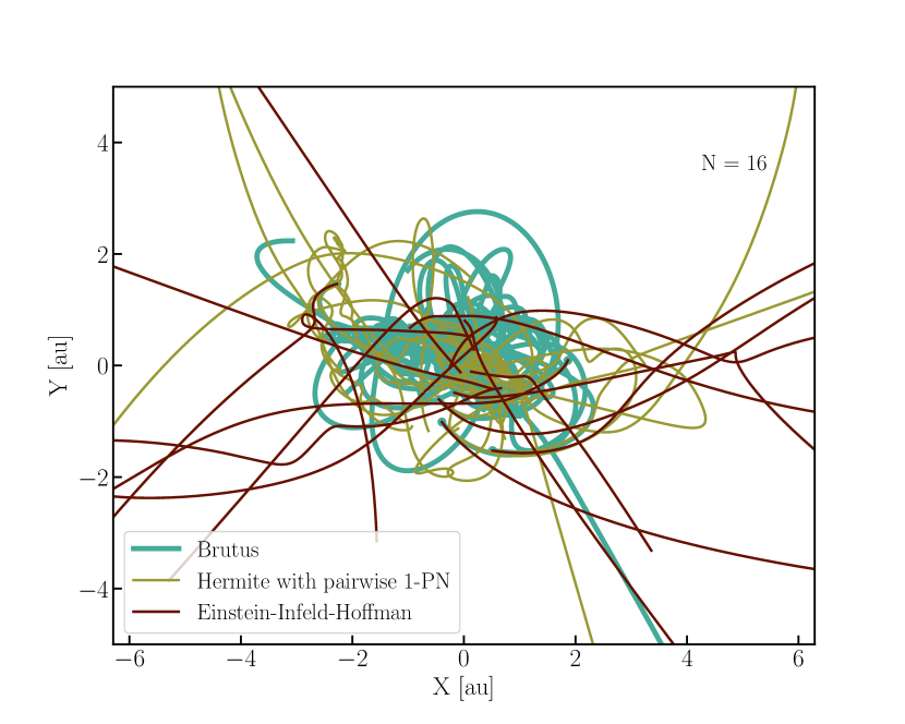
Figure 4: Orbital evolution of 16 of $10^{6}$ ${M}_{\odot}$  black holes with the same integrators as in fig. 2.

2.4 Initial conditions

Initial conditions were generated in standard IEEE double precision ($L_{w}=64$). This introduces a discrepancy with the low-$N$ $(\leq 64)$ experiments, for which the initial iteration was performed with $L_{w}=52$, but if convergence is already achieved for $\epsilon=10^{-10}$ ($L_{w}=72$), round-off at the 13th mantissa (the limiting precision for $L_{w}=52$) cannot have propagated to the first 3 decimal places.

We adopted the initial conditions from Goodman et al. (1993). All objects then have the same mass and are distributed in a unit cube in phase space (position and velocity) using dimensionless $N$-body units. After generating random positions and velocities, the system was moved to the center-of-mass frame and scaled to virial equilibrium for the Newtonian solution. The simulation runs with a finite speed of light also used the identical initial realizations as for the Newtonian case. The slight deviations from virial equilibrium in the relativistic initial conditions have no effect on our results because we started measuring the phase-space distance at $t=1$, and by that time, the system was well virialized. We validated and confirmed this statement by recalculating all simulations for $N=16$ with $v/c=0.01$, for which we scaled the initial conditions to virial equilibrium for $v/c=0.01$ by adapting masses and velocities according to Buchdahl (1964), however. The difference between the Newtonian and the relativistically virialized initial conditions was negligible.

The number of runs performed varied for each code and the number of particles, as listed in Table 1. In the second column, we list the number of runs performed with ph4. For the other runs, with Hermite_GRX  and Brutus,  the same initial realizations were adopted, but sometimes this was a subset. These calculations were performed up to $N=1$k using the same number of runs with the same initial conditions as in Goodman et al. (1993).

$N$	$N_{\rm runs}$
	ph4	Hermite_GRX	Brutus
3	100	—	—
4	200	200	200
8–64	100	100	100
128	20	10	10
256	10	10	3
512	10	2	2
1024	10	–	2
2048–16384	10	–	–
65536	6	–	–
131072	2	–	–

Table 1: Number of simulations performed per implementation and number of particles. The simulations for different codes use exactly the same initial realizations: The 200 initial realizations for $N=4$ are identical for the ph4, Brutus, and Hermite_GRX.

We performed an additional series of simulations using ph4  and Hermite_GRX, but with realizations generated using a Plummer (1911) sphere and a King model ($W_{o}=12$, King 1966).

The main reason not to perform larger simulations including the EIH equations is their unfavorite scaling of the computer time with $N$, which we depict in fig. 1. We estimate approximately one year of integration for $N\sim 10^{4}$ with the current CPU implementation.

2.5 Measuring the Lyapunov timescale

Measuring the Lyapunov timescale for the gravitational $N$-body system is not trivial. Several methods for deriving this quality have been proposed. One method uses the geodesic-deviation vector-technique (Weinberg 1972; Nieto et al. 2003) for two nearby orbits with projection operations and with time as an independent variable (Wu & Huang 2003), and the two-nearby realizations without projection operations and with time as an independent variable. We adopted the last, which may be more expensive to calculate, but is considerably simpler for large $N$, and it is least affected by underlying assumptions. This same technique was adopted in Goodman et al. (1993), which means that our analysis at least starts from the same assumptions. Strictly speaking, the Lyapunov timescale is defined properly from some starting point until the system dissolves (Urminsky & Heggie 2009; Mel’nikov et al. 2013). Because this definition is rather unpractical, particularly for large $N$, we stopped the calculations at $10\text{ }N$-body time units (equivalent to Goodman et al. 1993).

The degree of chaos in the simulation was measured using the evolution of the phase-space distance between two almost identical initial realizations (see § 2.4). The second realization was constructed by increasing the Cartesian $x$ coordinate of a randomly selected particle with a value of $10^{-7}$ (in dimensionless $N$-body units). Just to emphasize, this initial displacement is 10 million times shorter than the size of the initial extent of the $N$-body system. The perturbed realization is therefore not in strict equilibrium, but deviates from Newton’s equilibrium potential energy by ${\cal O}(10^{-7}/N^{2})$.

We integrated both initial realizations to $10\text{ }N$-body time units while saving a snapshot every $0.1N$-body time units, resulting in 100 snapshots per run. The phase-space distance was determined by taking the difference in position and velocity between the same particles in each snapshot, and summing them,

$$\ln(\delta)={1\over 2}\ln\left[\sum(\@vec{r}_{b}-\@vec{r}_{a})^{2}+(\@vec{v}_{b}-\@vec{v}_{a})^{2}\right].$$ (7)

This leads to a phase-space distance as a function of time. To calculate the Lyapunov exponent, we only used the data from $t=1$ to a maximum of either $t=10$, or the first moment in which the phase-space distance exceeded $0.1$. The choice of starting the Lyapunov timescale measurements at $t=1$ guarantees that the system is in virial equilibrium even in the most relativistic cases. We subsequently performed a least-squares fit to the phase-space distance evolution. The fitted slope (in $\log$ space) to this phase-space distance evolution gives the Lyapunov exponent. The Lyapunov timescale $t_{\lambda}$ is the reciprocal of the Lyapunov exponent.

This procedure is slightly different than what was used in Goodman et al. (1993), who adopted $t_{\lambda}=9/(\ln(\delta_{t=10})-\ln(\delta_{t=1}))$, but results in a better estimate of the global Lyapunov timescale. We stopped our measurement when $\delta\geq 0.1$ because due to conservation of the phase-space characteristics, the system then grows on a relaxation timescale, rather than on a Lyapunov timescale, and $\delta$ saturates when it becomes on the order of unity (Hut & Heggie 2002). For very chaotic systems, the procedure adopted by Goodman et al. (1993) leads to an underestimate of the Lyapunov exponent and therefore to an overestimate of $t_{\lambda}$, as is the case for $N\ga 1$k King models (see, e.g., in fig. 13).

3 Results

3.1 Chaos in large-$N$ Newtonian systems

In fig. 5 we show an example for an $1$k-body system, starting with the initial conditions of Goodman et al. (1993). The gray square in the middle represents these initial conditions; particles, according to Goodman et al. (1993), are initialized in a unit cube. One calculation (bullet points) gives the result of the unperturbed solution. The perturbed solution is not shown, but the colors of the particles give the phase-space distance between the final perturbed and unperturbed solutions. The black bullet point toward the top right corner of the gray area identifies the (randomly selected) particle for which the initial $x$-coordinate was increased by $10^{-7}$. The least (red) and most (blue) chaotic particles are represented as lines. The overplotted thin black curves show the orbit of the perturbed solution.

Figure 5 illustrates Miller’s (1964) point that a small perturbation in a single object leads to large variations in the final phase-space distribution. In fact, most objects experience a strong variation, whereas only a minority of objects are hardly affected. In fig. 6 we plot the distribution of phase-space distances ($\log_{10}(\delta)$) for the calculation of fig. 5.

Figure 5: Distribution of phase-space distances in a cluster with 1024 particles. Units are dimensionless N-body units (Hénon 1971). The gray shaded region indicates the initial conditions in a virialized unit cube. One particle, indicated with the black bullet point, is displaced by $10^{-7}$ along the Cartesian $x$ coordinate. The final conditions (at $t=10$) of the unperturbed particles are represented with the bullet points. The color and size of the points represents the phase-space distance measured over the duration of the simulation ($10\text{ }N$-body time units), and ranges over about four orders of magnitude. The majority of objects experience considerable change in their orbits, but some are hardly perturbed. Calculations were performed using Brutus  until convergence to 3 decimal places, which requires a tolerance of $\tau=10^{-40}$.

The degree to which particles are affected by a small initial perturbation depends on the number of particles in the system. This is illustrated in fig. 6, where we show the distribution of phase-space distance between a perturbed and an unperturbed solution for the same simulation as in fig. 5 using $1$k particles, and compare this distribution with $200$ simulations of $N=4$. The small-$N$ systems (red histogram) exhibits a much weaker response to a perturbing particle than the large-$N$ systems (blue); few-body systems are less chaotic than large-$N$ systems (at least for this selection of initial conditions, and under Newton’s forces).

Figure 6: Distribution of phase-space distances for individual particles $\delta_{i}$ in the simulations with $N=4$ (red) and those with $N=1024$ (blue) after integrating for $t=10$ $N$-body time units. The data for $N=4$ are the result of 200 runs. For $N=1024,$ we adopted the run used in fig 5. Calculations were performed using Brutus  until the solution was converged.

The different behavior for small-$N$ systems compared to large-$N$ systems motivated Goodman et al. (1993) and Hemsendorf & Merritt (2002) to conduct their analysis and study the source of chaos in small versus large $N$-body systems. In fig. 7 we show the results of Goodman et al. (1993) and compare them with converged solutions using Brutus  up to $N=1$k and reprehensible solutions using ph4  for up to $N=128$k. The consistency between the results obtained by Goodman et al. (1993) (red), Brutus  (blue), and ph4  (ochre) gives us confidence in the validity of the nonconverged (reprehensible) $N$-body solutions by Goodman et al. (1993) and using the regular Hermite algorithm implemented in ph4  without going through the elaborate process of reaching a converged solution for $N>1$k.

Figure 7: Estimate of the Lyapunov timescale as a function of the number of particles. Here the horizontal axis is not linear, but in $\ln(\ln(N))$ to illustrate the scaling proposed in Goodman et al. (1993). The different symbols and colors represent different calculations (see legend). The vertical bars, plotted for Newton’s Hermite only, show the root-mean-square of the dispersion in the series of solutions. The error bars in the results obtained with Brutus are statistically indistinguishable from the presented bars.

The scaling we observe in fig. 7 is consistent with that found by Goodman et al. (1993) over the entire range they explored, from $N=4$ to $N=512$. We therefore conclude that 1) reprehensible simulations are adequate for studying short-timescale Lyapunov exponent measurements for relatively homogeneous systems, and 2) the Lyapunov timescale $t_{\lambda}\propto\gamma t_{\rm cr}/\ln(\ln(N))$, with $\gamma=-1.39$ for $N\la 32$ and shallower with $\gamma=-0.498$ for $N\ga 32$.

3.2 Chaos in large-$N$ relativistic systems

To study the degree of chaos in the relativistic regime, we used the EIH equations of motion with initial realizations (masses, positions, and velocities) identical to those used in the Newtonian simulations. Therefore the latter initial conditions are in virial equilibrium for the Newtonian case, but not for the highly relativistic cases. Whereas the Newtonian $N$-body initial realizations and calculations were scale free, we have to relax this assumption when introducing the speed of light. Since our calculations scale with mass $M$, size $R$, or velocity $v$, we have the option to qualify the scaling by just changing $v/c$. Here $v/c\rightarrow 0$ corresponds to the Newtonian case (because in that case, $c\rightarrow\infty$); higher values of $v/c$ indicate a more relativistic regime.

We started by confirming that for $v/c\rightarrow 0,$ we reproduce the results from fig 7. As long as $v/c\la 10^{-4}$, the results of the relativistic integration can hardly be distinguished from the Newtonian case (see also figure 9).

This is further illustrated in figure 8, where we present two histograms for $N=4$ (red) and $N=64$ (blue) for $v/c=0.010$ (top panel) and $v/c=0.002$ (bottom). In the top panel, the distribution in phase-space distance for both $N=4$ and $N=64$ are comparable, although the dispersion for $N=64$ is somewhat larger. When we reduce the speed of light (expressed as the parameter $v/c$), both distributions move toward higher values of $\delta$. For $v/c=0.002$ (bottom panel), the systems, though still somewhat relativistic, have mean and median values that already approach the Newtonian values. We recall that with this adopted scaling, the system would correspond to a cluster with a total mass of $\sim 1$ ${M}_{\odot}$  at a size scale of $\sim 436$ au. Such a cluster of stars appears insufficiently relativistic for the degree of chaos in the equations of motion to be affected noticeably.

Figure 8: Distribution of phase-space distances for individual particles in the simulations with $N=4$ (red) and for $N=64$ (blue) after integrating for $t=10$ $N$-body time units. The data for 200 runs were used for each histogram. Calculations were performed using Hermite_GRX  using $v/c=0.01$ (top panel) and for $v/c=0.002$ (bottom panel).

However, for $v/c=0.0005$, which corresponds to a size scale four times larger, or equivalently, to a system four times more massive, the measurements in the Lyapunov timescale start to deviate from the Newtonian case. When we further decrease $v/c\la 10^{-4}$, the mean and median values of both distributions are statistically indistinguishable from the Newtonian case. The dispersion, particularly noticeable for $N=64$, remains skewed to low values of $\delta$.

In fig. 9 we present the median Lyapunov timescale for $N=4$ and $N=64$ as functions of $v/c$. For the asymptotic Newtonian case, $v/c\rightarrow 0$, the Lyapunov timescale converges to the median for the Newtonian case. The dispersion in the distribution in the relativistic case remains somewhat larger, however, even for $v/c\rightarrow 0$, for which $\langle t_{\rm Ly}\rangle=1.61\pm 2.36$, compared to the Newtonian case, for which $\langle t_{\rm Ly}\rangle=1.71\pm 1.68$.

We suspect that these small systematic effects (which are not statistically significant) could result from a few encounters sufficiently close to be affected by general relativity. For the extreme relativistic case, $v/c\ga 0.001$, the Lyapunov timescale rises quickly to $\langle t_{\rm Ly}\rangle=3.89\pm 0.64$. We present the results for $v/c\ga 0.02$ (two green points to the right), even though these are beyond the regime where the 1-PN Taylor-series expansion to the EIH equations of motion is valid (see sect. 4.2). We therefore limit further analysis to $v/c\la 0.010$.

For $N=4,$ we observed a minimum in the Lyapunov timescale for $v/c\sim 10^{-3}$ (signified by the horizontal dotted green line in fig. 9). The change in behavior for less and more relativistic systems might be interpreted as a signature that the adopted Taylor expansion starts to break down, but for $v/c\ga 10^{-3}$ , the post-Newtonian terms should still be valid. We expect the low-$N$ configurations to break down earlier when they are evolved with time because they are more relaxation dominated than the large-$N$ systems.

With a typical distribution in velocities matching a truncated Maxwellian, a small fraction ($\sim 2.9$ %) of the systems has a velocity that exceeds the mean dispersion by factor of 3. Even for a value of $v/c\ga 0.05,$ the fraction of stars with a velocity $v\ga 0.3c$ is smaller than $1/10^{7}$, and it is unlikely that when integrating over only 10 Hénon units, the post-Newtonian Taylor-series expansion breaks down.

Figure 9: Lyapunov timescale as a function of $v/c$ for $N=4$ (green) and $N=64$ (blue). The Newtonian case (run with ph4) is presented as arrows in orange. The vertical bars, only for the green points, indicate the dispersion in the simulation results. The short horizontal dotted green line indicates the lowest value for the Lyapunov timescale reached for $v/c=10^{-3}$ for $N=4$.

In fig. 10 we present measurements for the Lyapunov timescale for the post-Newtonian equations of motion. For $N\la 4$, the EIH equations of motion as well as the pairwise 1-PN terms show similar chaotic behavior in the sense that the relativistic system is less sensitive to initial perturbations than the Newtonian case. For $N\ga 20$, the pairwise 1-PN terms result in smaller Lyapunov timescales compared to Newton’s equations of motion, whereas the EIH equations of motion continue to result in a rather large Lyapunov timescale compared to the Newtonian case. The Lyapunov timescales for the EIH equations of motion are roughly twice as large as for the Newtonian case for $v/c=0.005$ and roughly four times as large for $v/c=0.010$.

Figure 10: Lyapunov timescale as a function of $N$ for Goodman et al. (1993) (red bullets) compared to the various relativistic solutions. In blue we present the solutions using 1-PN pair-wise terms with a scaling to the speed of light of $v/c=0.010$ and twice this value. For the EIH equations of motion we show the case for $v/c=0.010$ in green, twice and four times this value. The top blue curve fits $t_{\lambda}\simeq 0.255+13.43e^{-0.371N}$ for $v/c=0.005$, and $t_{\lambda}\simeq 0.051+5.50e^{-0.115N}$ for $v/c=0.010$.

The effect of $N$ on the degree of chaos in the equations of motion is further illustrated in figure 11. Here we show for $N=4$, $N=16,$ and for $N=64$ the ratio of the pairwise 1-PN solution as a function of the full EIH equations of motion. The relativistic calculations were performed with $v/c=0.010$.

For $N=4$, the Newtonian case shows a smaller average Lyapunov timescale than the two relativistic cases. This was also confirmed in the three-body simulations by Boekholt et al. (2021), who found no significant difference in the chaotic behavior of Newtonian versus relativistic systems. When $N$ increases, the distribution of the Lyapunov timescale for the EIH equations of motion continues to be large compared to the Newtonian case, but the value for the pairwise 1-PN terms tends to drop to less than 1/10th of the Newtonian solution. We conclude that if one is interested in the dynamical behavior of $N\ga 4$ black holes, the pairwise 1-PN terms do not reliably represent the chaotic behavior expected for such a relativistic system. The pairwise 1-PN terms address pairs of compact objects, whereas the EIH equations of motion should give a more reliable representation for relativistic systems of $N\geq 3$. We expect this difference to persist for the higher-order Taylor expansion terms.

Figure 11: Estimate for the Lyapunov timescale for the pairwise 1-PN terms as a function of the full EIH equations of motion for three choices of $N$, 4 (dark blue), 16 (aquamarine), and 64 (green). Both, the pairwise 1-PN calculation and the one including the cross terms, are represented as fraction of the Newtonian solution. All relativistic simulations adopt $v/c=0.010$.

4 Discussion

4.1 Consequences of the 1-PN terms

Phase-space volume is preserved in a solution to a conservative Hamiltonian system, but shrinks in a dissipative system (Shivamoggi 2014), as is the case in general relativity. The contraction of the phase-space volume gives rise to an attractor, and as a consequence, can have bounded trajectories (Bergé et al. 1987). It is not a priori clear, however, how dissipation in an otherwise conservative system affects chaotic motion (Lakshmanan & Rajasekar 2003). We find that in the conservative 1-PN regime, the chaotic behavior of N-body systems is already affected. In particular, for $N\ga 10$, simulations that only include the 1-PN pairwise terms behave differently than when the 1-PN cross-terms for the EIH equations of motion are incorporated into the simulations. The behavior of relativistic systems with $v/c\ga 0.005$ and for $N\ga 10$ is considerably less chaotic than their less-relativistic $v/c\la 10^{-3}$ and Newtonian counterparts.

4.2 Validity of the post-Newtonian terms

In this study, we rely on the post-Newtonian expansion of the EIH equations of motion. Ideally, we would have adopted full general relativity in our $N$-body calculations, but this is somewhat beyond the scope of our study and is numerically challenging.

In an attempt to quantify the validity of the post-Newtonian expansion adopted here, we compared the apsidal motion of the orbit-averaged evolution for a two-body system with total mass $M$, semimajor axis $a,$ and eccentricity $e$. We write the relative velocity in a circular orbit in terms of the gravitational radius, $r_{g}=GM/c^{2}$ , and the speed of light as

$$c\simeq\sqrt{GM/(10r_{g})}.$$ (8)

The Taylor-series expansion then starts to break down for $v\equiv c/\sqrt{10}\sim 0.3c$ (Will 2011). During our $N$-body calculations, we kept track of this velocity to ensure that the Taylor series expansion in our calculations remained reliable. However, this safety check does not guarantee that our results are not affected, particularly for high values of $v/c$.

In the regime in which the Taylor-series expansion of the EIH equations of motion breaks down, the 1-PN terms adopted here are insufficient to capture the correct physical behavior. In this case, the 2-PN terms become essential for the correct physical interpretation of the numerical results. By definition, the 2-PN terms are smaller than the 1-PN terms because the former scale as $v/c$ and the latter as $v^{2}/c^{2}$. On the other hand, both terms approach each other for more relativistic systems, with $v\rightarrow c$. It is somewhat tricky to give an absolute measure when the 2-PN terms should be used in addition to the 1-PN terms. In a general $N$-body problem, stars may approach each other at a short distance with relatively high velocities with respect to $c$. When such an encounter is a one-time event in the nondissipative limit, the lack of precision in the PN terms is not expected to make a great difference in the eventual results (Will 2011). Reprehensive simulations are therefore sufficient to derive the largest global positive Lyapunov exponent for the system.

In an attempt to quantify the relative importance of 1-PN with respect to the 2-PN terms, we compared the apsidal motion of the orbit-averaged evolution for a two-body system with a total mass $M$, semimajor axis $a,$ and eccentricity $e$. We write (Iorio 2020)

$$\dot{\omega}_{2PN}/\dot{\omega}_{1-PN}\simeq(r_{g}/a)(1/12)(28-e^{2})/(1-e^{2}).$$ (9)

In fig. 12 we show as a function of $v/c$ the relative drift in the apsidal motion for the 1-PN and 2-PN terms for two bodies in a circular orbit at $100r_{g}$,

$$v/c = (1/c)\sqrt{GM/a}\sqrt{(1+e)/(1-e)}.$$ (10)

The boundary at which the post-Newtonian expansion is no longer reliable is indicated by the dashed vertical line, near $v/c\simeq 0.4$, which happens when the two objects approach within $10r_{g}$. If we compare this boundary to the range in $v/c$ in figure 9, we find that all lie below the boundary, and we therefore argue that the increase in the Lyapunov timescale toward the relativistic regime is physical and not a numerical artifact.

Figure 12: Relative importance in the apsidal motion of the 1-PN terms in comparison to the 2-PN terms.

4.3 Other initial density profiles

The initial conditions adopted in Goodman et al. (1993) have a homogeneous phase-space distribution within the adopted limits, and they do not represent any observed stellar systems (Portegies Zwart et al. 2010). Clusters of stars are better represented with a Plummer (1911) distribution or a King (1966) model. For this reason, we also performed a series of calculations with these distributions. One series of Newtonian calculations used Plummer models and King models with dimensionless depth of $W_{0}=12$ (which is rather concentrated), and one set of calculations used the EIH equations of motion for the King model case (with identical initial realizations).

In figure 13 we present the Lyapunov timescales for these simulations as functions of $N$. The Newtonian Plummer case shows a slightly smaller Lyapunov timescale than the homogeneous distribution used in Goodman et al. (1993). The Plummer distribution is consistent with the initial conditions adopted by Hemsendorf & Merritt (2002), and their results are consistent with our results for the Plummer sphere, see figure 13 (black points).

Figure 13: Estimated Lyapunov timescale for the Newtonian case with particles distributed in a Plummer sphere (blue) and a King model (yellow). In addition, we show results for the King model, but for the EIH equations of motion with $v/c=0.010$ (green). Here the $x$-axis is in $\ln(\ln(N))$.

The Newtonian King model with $W_{0}=12$ is considerably more chaotic than the homogeneous initial realization adopted in Goodman et al. (1993), at least given that for $N\ga 10^{3}$ we were unable to measure a reliable Lyapunov timescale because the phase-space distance grew beyond $\delta=0.1$ within 1 $N$-body time unit. King models with a central potential depth of $W_{0}=12$ turn out to be considerably more chaotic than Plummer models (for $N\ga 40$), while Plummer models are expected to behave more chaotically than a homogeneous distribution of particles. This is not a complete surprise because the choice of $W_{0}=12$ places the model near core collapse (at least in its density profile). The growth of an initial phase-space distance between two subsequent calculations with almost identical initial relations is then dominated by few-body interactions in the core. One could argue that the entire chaotic behavior of the star cluster is driven by few-body interactions in the cluster center. Since some complex three-body interactions are fundamentally unpredictable (Boekholt et al. 2020), the dynamical evolution of the entire cluster will be unpredictable.

The extreme relativistic case, with $v/c=0.01$, shows a similar characteristic again as the homogeneous initial realizations, but a rather different scaling when adopting the King model. In the Newtonian case, King models tend to have considerably smaller Lyapunov timescales, but when extremely relativistic, they tend to be more regular than the Newtonian case Fig 10.

5 Conclusions

We have numerically analyzed the rate at which neighboring solutions of the equations of motion for $N$ self-gravitating bodies diverge in the Newtonian regime, but also with the 1-post-Newtonian expansion terms for the pairwise approximation and the Einstein-Infeld-Hoffmann equations of motion. Our results can be interpreted as the rate of growth of the error in an $N$-body solution, caused by uncertainties in the initial conditions or errors produced numerically during integration.

Our Newtonian simulations were repeated with higher precision and accuracy until a converged solution was achieved. Due to computer limitations, this was performed for $N$ up to $1024$ particles. For large particle numbers (and for the relativistic simulations), we used reprehensible $N$-body solutions, and we confirmed them to be veracious for $N$ up to $1$k particles.

The motivation to study the growth of errors stems from our desire to understand the role of chaos in these systems. The macroscopic distribution of material in the Galaxy may not be affected by microscopic chaos. But the Galaxy is built up of small subsystems of stars, each of which exhibits chaotic behavior, and the range of the Newtonian force law causes chaos in these microscopic systems to propagate to the Galaxy at large. Chaos in the Galaxy is then governed by the chaos in small $N$ subsystems and not by the global slow (on timescales longer than the dynamical timescale) variations of the orbits of stars in a smooth potential.

We confirm the earlier result of Goodman et al. (1993) and Hemsendorf & Merritt (2002) that the divergence in $N$-body systems grows exponentially, with an e-folding timescale on the order of the crossing time. Our results agree with the $t_{\lambda}\propto t_{\rm cross}/\ln(\ln(N))$ scaling of Goodman et al. (1993) and are inconsistent with a $t_{\rm cross}/\ln(N)$ scaling.

Our conclusions are listed below.

1. For a homogeneous distribution of equal-mass particles in virial equilibrium, the e-folding timescale for the growth of an initial perturbation in an $N$-body system, the so-called Lyapunov timescale, scales for small systems of $N\la 32$ as $t_{\lambda}/t_{\rm cross}=(0.88\pm 0.12)-(1.39\pm 0.13)\ln(\ln(N))$. For larger systems of $N\ga 32$, the Lyapunov timescale scales as $t_{\lambda}/t_{\rm cross}=(-0.094\pm 0.129)-(0.498\pm 0.066)\ln(\ln(N))$.

2. For an initial Plummer distribution, the e-folding timescale is smaller than the homogeneous initial realizations by about a factor of $5$ but preserves the same trend, or for $N\ga 32,$ it fits $t_{\lambda}/t_{\rm cross}=(-0.475\pm 0.018)-(0.528\pm 0.010)\ln(\ln(N))$.

3. For more concentrated models, such as a King model with $W_{0}=12$, the scaling is comparable to the slope observed in the homogeneous unit-cube or the Plummer distribution, with $t_{\lambda}/t_{\rm cross}=(1.346\pm 0.110)-(2.212\pm 0.107)\ln(\ln(N))$, but extending somewhat farther, to $N\simeq 64$. For larger $N,$ the slope is much steeper, $t_{\lambda}/t_{\rm cross}=(4.970\pm 2.03)-(4.813\pm 1.147)\ln(\ln(N))$, indicating that these systems are chaotic for large $N$ on a timescale smaller than a crossing time.

4. If a small perturbation is introduced into a single particle of a large $N$-body system, all particles are affected within a few crossing times.

5. For self-gravitating systems with $v/c\la 10^{-3}$, the phase-space mixing of relativistic $N$-body systems is indistinguishable from the Newtonian case. This limit is already reached for a total of ten  black holes of 10 ${M}_{\odot}$  confined to a spherical volume of radius $10^{-3}$ pc.

6. For highly relativistic systems, $v/c\ga 0.002$, the EIH equations of motion to 1-PN are considerably less chaotic than their Newtonian counterpart over all values of $N$. The Lyapunov timescale scales with $t_{\lambda}/t_{\rm cross}=6.63\pm 1.68-\ln\left(3.72\pm 2.04\ln(N)\right)$.

7. For small $N$ ($\la 10$), the pairwise 1-PN terms give similar phase-space mixing to the EIH equations of motion.

8. For $N>4$, the pairwise 1-PN corrected equations of motion become considerably more sensitive to perturbations in the initial conditions compared to the EIH equations of motion. The former show considerably shorter Lyapunov timescales compared to their Newtonian counterparts, whereas the latter has even longer Lypaunov timescales.

9. We conclude that the Galaxy is intrinsically chaotic on a very short timescale because of the chaotic behavior of microscopic few-body interactions in the centers of star clusters. The chaotic behavior of these small-$N$ systems propagates on a local crossing timescale to the entire star cluster, affecting the orbits of neighboring stars and clusters, and eventually, the entire Galaxy.

10. The pairwise terms for $N>3$ give a different dynamical behavior for relativistic $N$-body systems compared to the full EIH equations of motion.

Considering the effect of the full EIH equations of motion on a relativistic cluster of compact objects, and the potential consequences for observations with laser interferometric gravitational wave observatories, we look forward to implementing and study the effect of higher-order cross-terms in general relativistic $N$-body simulations. We do realize, however, that these calculations do not have the most favorable scaling of the computer time with respect to $N$.

Public data

The source code, input files, simulation data, and data processing scripts for this manuscript are available at figshare under DOI 10.6084/m9.figshare.xxxx.

Software used for this study

This work would have been impossible without the following public open-source packages and libraries: Python (van Rossum 1995), matplotlib (Hunter 2007), numpy (Oliphant 2006), MPI (Gropp et al. 1996; Gropp 2002), and AMUSE (Portegies Zwart et al. 2018, available for download at https://amusecode.org). Sapporo  GPU library (Portegies Zwart et al. 2007; Gaburov et al. 2009), MPFR library (Fousse et al. 2007) of the GMP library (Granlund & the GMP development team 2012).

A (python notebook) tutorial for students is available at https://github.com/amusecode/Tutorial. All the $N$-body codes used in this study are available in the AMUSE repository at amusecode.org.

Appendix A Implementation of the numerical method

The Newtonian solver and the post-Newtonian terms are implemented in C and C++ and interfaced with the Astrophysics Multipurpose Software Environment (AMUSE for short, Portegies Zwart & McMillan 2018). In this appendix, we discuss the simple Hermite predictor-corrector Newtonian $N$-body solver called ph4  and the post-Newtonian solver called Hermite_GRX. The former solves Newton’s equations of motion quite accurately, but is unable to achieve converged solutions. The other code adopts the post-Newtonian approach in which we address the pairwise EIH equation as well as the so-called cross-terms (Einstein et al. 1938). All equations are implemented to 1-PN order.

The Newtonian code, ph4, is optimized for parallel operations using the Message Passing Interface (MPI, Gropp et al. 1996; Gropp 2002), and for GPU using the Sapporo  library (Portegies Zwart et al. 2007; Gaburov et al. 2009). The post-Newtonian implementation, Hermite_GRX  is parallelized using hyperthreading, but not using MPI, and it does not support GPU operations. In this code, however, few-body interactions are regularized using quaternions.

In the following sections, we discuss the various implementations and optimizations. We also perform some test calculations to demonstrate the efficiency and accuracy of the various implementations.

A.1 Fourth-order Hermite integration scheme

Here we describe the fourth-order Hermite predictor corrector implementation in ph4  and Hermite_GRX  briefly. The first solves Newton’s equations of motion; the second also includes various solvers for addressing the post-Newtonian expansion terms.

A.1.1 Predict, evaluate, and correct scheme

The Hermite integration scheme is a family of implicit numerical methods for solving ordinary differential equations. Introduced by Makino (1991), the fourth-order integration scheme is written

$$y(t+h) = y(t)+\frac{y^{(1)}(t)+y^{(1)}(t+h)}{2}h$$

$$+\frac{y^{(2)}(t)-y^{(2)}(t+h)}{12}h^{2}+\mathcal{O}\left(h^{5}\right),$$

which has a local truncation error of $\mathcal{O}\left(h^{5}\right)$, resulting in a global truncation error of $\mathcal{O}\left(h^{4}\right)$. We denote the $i$-th derivative with respect to $t$ using $(\cdot)^{(i)}$ or with Einstein’s convention. The sixth- and eight-order schemes, derived by Nitadori & Makino (2008), are not implemented here.

Because the scheme is implicit, a fixed-point iteration to solve eq. A.1.1 is needed,

$$y_{[i+1]}(t+h) = y(t)+\frac{y^{(1)}(t)+y_{[i]}^{(1)}(t+h)}{2}h$$

$$+\frac{y^{(2)}(t)-y_{[i]}^{(2)}(t+h)}{12}h^{2}.$$

Here we used a truncated Taylor expansion around $t$ as the initial (boundary) condition

$$y_{[0]}(t+h)=y(t)+hy^{(1)}(t)+\frac{h^{2}}{2}y^{(2)}(t).$$ (13)

This sequence converges to the limit $y(t+h)$, which ends the current time step. In practice, a single iteration suffices when the time step $h$ is small.

Each integration step then consists of

1. prediction of the positions and velocities at the next time step $t+h$,

   $$\tilde{\boldsymbol{r}}_{i+1}=\boldsymbol{r}_{i}+\boldsymbol{v}_{i}h+\tfrac{1}{2}\tilde{\boldsymbol{a}_{i}}h^{2}+\tfrac{1}{6}\boldsymbol{j}_{i}h^{3},$$ (14a)

   $$\tilde{\boldsymbol{v}}_{i+1}=\boldsymbol{v}_{i}+\boldsymbol{a}_{i}h+\tfrac{1}{2}\boldsymbol{j}_{i}h^{2}.$$ (14b)

   Here $\boldsymbol{r}$, $\boldsymbol{v}$, $\boldsymbol{a}$, and $\boldsymbol{j}=\frac{\mathrm{d}\boldsymbol{a}}{\mathrm{d}t}\equiv\dot{a}$ represent vectors for the position, velocity, acceleration, and jerk, respectively. The jerk $\@vec{j}$ is dotted, which in this case does not indicate a time derivative. Predicted values are indicated with the $\tilde{(\cdot)}$.

2. Acceleration and jerk are calculated using the predicted positions and velocities (eq. 14).

3. A subsequent correction is applied to the position and velocity at the next time step using the predicted accelerations and jerks,

   $$\boldsymbol{v}_{i+1}=\boldsymbol{v}_{i}+\tfrac{1}{2}(\boldsymbol{a}_{i}+\tilde{\boldsymbol{a}}_{i+1})h+\tfrac{1}{12}(\boldsymbol{j}_{i}-\tilde{\boldsymbol{j}}_{i+1})h^{2},$$ (15a)

   $$\boldsymbol{r}_{i+1}=\boldsymbol{r}_{i}+\tfrac{1}{2}(\boldsymbol{v}_{i}+\boldsymbol{v}_{i+1})h+\tfrac{1}{12}(\boldsymbol{a}_{i}-\tilde{\boldsymbol{a}}_{i+1})h^{2}.$$ (15b)

The corrected velocities increase the order of the method to $\mathcal{O}\left(h^{4}\right)$. In such a predict, evaluate, and correct (PEC) scheme, the fixed-point iteration can be described as $P(EC)^{n}$ for $n$ iterations.

A.1.2 Variable time step

We use variable but shared time steps. After every step, a new time-step size is determined based on the minimum interparticle collision timescale, calculated from unaccelerated linear motion and the freefall time,

$$h=\eta\min_{i,j\not=i}{\left(\frac{|\boldsymbol{r}_{ij}|}{|\boldsymbol{v}_{ij}|},\frac{|\boldsymbol{r}_{ij}|}{|(m_{i}+m_{j})\boldsymbol{a}_{ij}|}\right)}.$$ (16)

Here $r_{ij}$, $v_{ij}$, $a_{ij}$ are the relative distance, velocity, and acceleration between particles $i$ and $j$, and $m_{i}$ is the mass of particle $i$. The minimum is taken over each pair of particles $(i,j)$, and over the two estimates of the collision time. Here the time-step parameter $\eta$ is introduced to control the time-step size and therewith the accuracy (and speed) of the integration scheme. Ler values of $\eta$ generally correspond to smaller errors and a longer integration wall-clock time. The default value in AMUSE, $\eta=0.03$, generally leads to acceptable accuracy at a reasonable speed: in many cases, $\eta=0.1$ probably suffices (Portegies Zwart & Boekholt 2014). For safety, we adopted $\eta=0.01$ for our calculations.

The adopted variable time step removes the time-symmetric properties of the integration. The fundamental idea behind time-symmetrization is to prevent systematic drift in any conserved quantity. Time reversibility then introduces the same drift with opposite sign.

A time-symmetric algorithm exhibits the same drift in both directions of time, resulting in identical absolute drifts when integrating forward and backward with time. This is a desirable quality of an integrator because we consider Nature to conserve energy and angular momentum (see also Portegies Zwart & Boekholt 2018, for a discussion on the arrow of time due to the chaotic behavior of self-gravitating systems and uncertainties on the smallest scales).

One can reintroduce time-symmetry by selecting a symmetric time step, for example, by taking the average of some function at either side of the integration step (Hut et al. 1995),

$$h=\tfrac{1}{2}(k(t_{b})+k(t_{e})).$$ (17)

Here $k(t)$ is a function to determine the step size at the beginning $t_{b}$ and at the end $t_{e}=t_{b}+h$ of the integration step. This implicit expression requires fixed-point iteration to evaluate

$$h_{[0]}=k(t_{b}),$$ (18a)

and the eventual time step when the sequence converges becomes

$$h_{[i+1]}=\tfrac{1}{2}\left(k(t_{b})+k(t_{b}+h_{[i]})\right).$$ (19a)

Generally, the sequence converges in a single iteration (Hut et al. 1995).

A.1.3 Splitting the jerk

Calculating the jerk is expensive in terms of computer time because it requires three passes over all particles. To avoid evaluating the jerk directly, we use a central numerical derivative,

$$\boldsymbol{j}(t)=\frac{\boldsymbol{a}(t+h)-\boldsymbol{a}(t-h)}{2h}+\mathcal{O}\left(h^{2}\right).$$ (20)

Here the accelerations are calculated using the Taylor expanded positions and velocities of the particles,

$$\boldsymbol{r}(t\pm h)=\boldsymbol{r}(t)\pm h\boldsymbol{v}(t)+\tfrac{1}{2}h^{2}\boldsymbol{a}(t)+\mathcal{O}\left(h^{3}\right),$$ (21a)

$$\boldsymbol{v}(t\pm h)=\boldsymbol{v}(t)\pm h\boldsymbol{a}(t)+\mathcal{O}\left(h^{2}\right).$$ (21b)

The numerical calculation of the jerk is equally expensive as the analytic calculation because it requires two additional acceleration calculations per jerk. We reduce the computational complexity by the time step $h$ of the previous integration step and the backward derivative. This allows us to reuse the previous steps’ positions and velocities for calculating the jerk at the current time step.

Using a first-order derivative instead of the analytical expression for the jerk leads to a reduced accuracy, but this is corrected for by splitting the acceleration into two parts: the Newtonian part, and a perturbing part,

$$\boldsymbol{a}(t)=\boldsymbol{a}_{\mathrm{Newton}}(t)+\boldsymbol{a}_{\mathrm{pert}}(t).$$ (22)

We note here that we already introduced a perturbation, which in the EIH equations of motion will be the post-Newtonian terms. The Newtonian jerk can now be calculated analytically and at negligible cost compared to calculating the perturbing acceleration. The perturbing jerk is calculated from the numerical backward derivative,

$$\boldsymbol{j}(t)=\boldsymbol{j}_{\mathrm{Newton}}(t)+\frac{\boldsymbol{a}_{\mathrm{pert}}(t)-\boldsymbol{a}_{\mathrm{pert}}(t-h)}{h}+\mathcal{O}\left(h^{2}\right).$$ (23)

This operation increases the memory requirement by storing two accelerations for each particle.

The algorithm is made to be self-starting by defining the perturbing acceleration of the previous integration step $\boldsymbol{a}_{i-1,\mathrm{pert}}$, as it depends on the jerk of the first iteration $\boldsymbol{j}_{i}$. For this, we chose $\boldsymbol{a}_{i-1,\mathrm{pert}}=\boldsymbol{a}_{i,\mathrm{pert}}$, so that $\boldsymbol{j}_{i,\mathrm{pert}}=0$. This decreases the local truncation error of the first step to $\mathcal{O}\left(h^{4}\right)$, but its impact on the results is small because only one step is taken.

A.2 Regularization

Regularizing the equations of motion for two bodies (or more) in a close encounter improves computational performance and accuracy. The main reason to introduce regularization, however, is to prevent a devision by zero for extremely close approaches between particles (Kustaanheimo & Stiefel 1965; Mikkola & Tanikawa 1999). Regularizing the post-Newtonian expressions is harder than the regular Newtonian case because of the velocity dependence on the acceleration (Mikkola & Merritt 2006, 2008a). Here we derive the regularized equations of motion in post-Newtonian few-body encounters using quaternions (Waldvogel 2006), but we start with a brief overview on quaternions

A.2.1 Quaternions

Quaternions are an extension of complex numbers to three complex base quaternions $\boldsymbol{i}$, $\boldsymbol{j}$ , and $\boldsymbol{k}$ (Waldvogel 2006). A quaternion $\boldsymbol{u}$ is constructed from four real numbers $u_{\ell}\in\mathbb{R}$ for $\ell=0,1,2,3$,

$$\boldsymbol{u}=u_{0}+u_{1}\boldsymbol{i}+u_{2}\boldsymbol{j}+u_{3}\boldsymbol{k},$$ (24)

with the multiplicative identities

$$\boldsymbol{i}\boldsymbol{i}=\boldsymbol{j}\boldsymbol{j}=\boldsymbol{k}\boldsymbol{k}=\boldsymbol{i}\boldsymbol{j}\boldsymbol{k}=-1,$$ (25)

from which we derive the other products,

$$\cases{}{i}\boldsymbol{j}$$ =-ji=k, (26)

(27)

(28)

From these, the noncummatative property of quaternion multiplication is evident. We define the conjugate of quaternion $\boldsymbol{u}$,

$$\overline{\boldsymbol{u}}=u_{0}-u_{1}\boldsymbol{i}-u_{2}\boldsymbol{j}-u_{3}\boldsymbol{k},$$ (29)

which leads to the definition of the norm

$$|\boldsymbol{u}|^{2}=\boldsymbol{u}\overline{\boldsymbol{u}}=\overline{\boldsymbol{u}}\boldsymbol{u}=u_{0}^{2}+u_{1}^{2}+u_{2}^{2}+u_{3}^{2}.$$ (30)

The star conjugate of $\boldsymbol{u}$ then is

$$\boldsymbol{u}^{\star}=u_{0}+u_{1}\boldsymbol{i}+u_{2}\boldsymbol{j}-u_{3}\boldsymbol{k}.$$ (31)

We associate the vector $\boldsymbol{r}=(r_{0},r_{1},r_{2})\in\mathbb{R}^{3}$ to quaternion $\boldsymbol{u}$ as

$$\boldsymbol{u}=r_{0}+r_{1}\boldsymbol{i}+r_{2}\boldsymbol{j}.$$ (32)

When describing real-world coordinates, quaternions have a vanishing component in $\boldsymbol{k}$ (Waldvogel 2006).

A.2.2 Equations of motion

Regularization is applied to pairs of particles. They, particle $i=1$ and $i=2$, are located at phase-space coordinate $\boldsymbol{r}_{i}$ with velocities $\boldsymbol{v}_{i}$, and masses $m_{i}$. The equations of motion are

$$\ddot{\boldsymbol{r}}_{i}=-\frac{Gm_{j}}{r^{3}}(\boldsymbol{r}_{j}-\boldsymbol{r}_{i})+\boldsymbol{a}_{i}.$$ (33)

The acceleration $\boldsymbol{a}_{i}$ for particle $i$ consists of all perturbing (post-Newtonian) and Newtonian accelerations, excluding the Newtonian acceleration between particle $i$ and $j$. The center of mass

$$\boldsymbol{r}_{\mathrm{cm}}=\frac{m_{1}\boldsymbol{r}_{1}+m_{2}\boldsymbol{r}_{2}}{m_{1}+m_{2}},$$ (34)

and the relative position

$$\boldsymbol{r}_{12}=\boldsymbol{r}_{2}-\boldsymbol{r}_{1},$$ (35)

we rewrite these equations of motion as

$$\ddot{\boldsymbol{r}}=-\frac{\mu}{r^{3}}\boldsymbol{r}+\boldsymbol{P},$$ (36)

and

$$\ddot{\boldsymbol{r}}_{\mathrm{cm}}=\frac{m_{1}\boldsymbol{a}_{1}+m_{2}\boldsymbol{a}_{2}}{m_{1}+m_{2}}.$$ (37)

Here $\mu=G(m_{1}+m_{2})$ is the gravitational parameter, and $\boldsymbol{P}=\boldsymbol{a}_{2}-\boldsymbol{a}_{1}$ the relative perturbing acceleration.

The above equations of motion have a singular point at $r=0$. We integrate the center of mass separately from the relative position, and rewrite the equation of motion in such in a way as to remove this singular point. This is achieved by remapping the world position to a regularized position quaternion $\boldsymbol{u}$, from which we calculate the world position

$$\boldsymbol{r}=\boldsymbol{u}\boldsymbol{u}^{\star}.$$ (38)

The quaternion $\boldsymbol{r}$ now has vanishing component $\boldsymbol{k}$ and can therefore be transformed into a vector, from which it follows that

$$r=|\boldsymbol{r}|=|\boldsymbol{u}|^{2}=\boldsymbol{u}\overline{\boldsymbol{u}}.$$ (39)

A (nonunique) solution to the inverse of eq. 38 is

$$\hat{\boldsymbol{u}}=\frac{\boldsymbol{r}+|\boldsymbol{r}|}{\sqrt{2(|\boldsymbol{r}|+r_{0})}}.$$ (40)

The position vector, $\boldsymbol{r}$, is almost entirely oriented in the negative $r$-direction, and the denominator is close to zero. Without loss of generality, we can avoid large numerical errors by swapping indices $i=1$ and $2$, resulting in the negation of $\boldsymbol{r}$.

The regularization time $\tau$ is

$$\mathrm{d}t=r\leavevmode\nobreak\ \mathrm{d}\tau.$$ (41)

The equations of motion for the regularized position is written in regularized time:

$$\boldsymbol{u}^{(2)}=-\tfrac{1}{2}b\boldsymbol{u}+\tfrac{1}{2}r\boldsymbol{P}\overline{\boldsymbol{u}}^{\star}.$$ (42)

Here $b$ is the binding energy of the binary,

$$b=\frac{\mu}{r}-\frac{1}{2}|\dot{\boldsymbol{r}}|^{2}\;\;\;=\;\;\;\frac{\mu-2|\boldsymbol{u}^{(1)}|^{2}}{|\boldsymbol{u}|^{2}}.$$ (43)

For an unperturbed two-body system, $\boldsymbol{P}=0$, the binding energy $b$ is constant, and the equation of motion describes the harmonic oscilator. For a perturbed two-body system, the expression resembles a perturbed harmonic oscilator. The greatest advantage of this approach is that this equation of motion has no singular points, not even for $r=|\boldsymbol{u}|^{2}=0$. This improves the performance for small perturbations when numerically integrating the equations of motion of a highly eccentric binary, and it improves the accuracy for perturbed binaries.

The binding energy (eq. 43) is not regularized, and errors continue to increase in close encounters (Funato et al. 1996a). This problem is mitigated by also integrating the binding energy numerically. When the binding energy changes slowly with time as a function of the perturbing accelerations, we find

$$b^{(1)}=-\langle\boldsymbol{r}^{\prime},\boldsymbol{P}\rangle.$$ (44)

Here the $\langle(\cdot),(\cdot)\rangle$ is the vectorial scalar product. An initial condition for $\boldsymbol{u}^{(1)}$ is

$$\hat{\boldsymbol{u}}^{(1)}=\tfrac{1}{2}\boldsymbol{v}\overline{\boldsymbol{u}}^{\star}.$$ (45)

This expression gives a small correction to the original derivation by Waldvogel (2006) and Waldvogel (2008): it can be verified by substitution in eq. 43, to derive the binding energy in world coordinates. For the reciprocal eq. 45, the right-hand side multiplication with $\boldsymbol{u}^{\star}$ leads to

$$\boldsymbol{v}=\tfrac{2}{r}\dot{\boldsymbol{u}}\boldsymbol{u}^{\star}\equiv\tfrac{2}{r}\boldsymbol{u}^{(1)}\boldsymbol{u}^{\star}.$$ (46)

One can also formulate the Kustaanheimo-Stiefel (hereafter KS Kustaanheimo & Stiefel 1965) regularized equations of motion in terms of the perturbing potential (Stiefel & Scheifele 1975), which can be advantageous in some cases, although it only applies to cases when the potential is independent of velocity (not the case for general relativity). Moreover, Stiefel and Steifele (1975, see pages 30 and 31) argued that it is numerically more efficient to formulate the equations of motion in terms of the total energy, not just the Kepler energy (see their eq. (A.31)). The equations of motion can also be cast into the form of regular elements (Stiefel & Scheifele 1975, their pages 90 and 91) that are advantageous for perturbed two-body systems because the regular elements remain exactly constant for nonperturbed systems (i.e., the two-body system is integrated analytically).

A.2.3 Numerical integration

We solve the equations of motion using the Hermite scheme in the PEC formulation (see sect. A.1.1), with $\Delta\tau\equiv\kappa$. The resulting intergration scheme is described below.

1. Predict the regularized position, regularized velocity, and binding energy at the end of the current integration step,

   $$\tilde{\boldsymbol{u}}_{i+1}=\boldsymbol{u}_{i}+\boldsymbol{u}^{(1)}_{i}\kappa+\tfrac{1}{2}\boldsymbol{u}^{(2)}_{i}\kappa^{2}+\tfrac{1}{6}\boldsymbol{u}^{(3)}_{i}\kappa^{3},$$ (47a)

   $$\tilde{\boldsymbol{u}}^{(1)}_{i+1}=\boldsymbol{u}^{(1)}_{i}+\boldsymbol{u}^{(2)}_{i}\kappa+\tfrac{1}{2}\boldsymbol{u}^{(3)}_{i}\kappa^{2},$$ (47b)

   $$\tilde{b}_{i+1}=b_{i}+b^{(1)}_{i}\kappa+\tfrac{1}{2}b^{(2)}_{i}\kappa^{2}.$$ (47c)

   Then predict the center-of-mass position and velocity from eq. 14.

2. Evaluate the regularized acceleration, regularized jerk, and the derivatives of the binding energy at the end of the current integration step, according to eqs. 42 and 44,

   $$\boldsymbol{u}^{(3)}=\tfrac{1}{2}\left(-b^{(1)}\boldsymbol{u}-b\boldsymbol{u}^{(1)}+r^{(1)}\boldsymbol{P}\overline{\boldsymbol{u}}^{\star}+r\boldsymbol{P}^{(1)}\overline{\boldsymbol{u}}^{\star}+r\boldsymbol{P}(\overline{\boldsymbol{u}}^{(1)})^{\star}\right),$$ (48a)

   $$b^{(2)}=-\langle\boldsymbol{r}^{(2)},\boldsymbol{P}\rangle-\langle\boldsymbol{r}^{(1)},\boldsymbol{P}^{(1)}\rangle.$$ (48b)

   The test-particle integrator by Hamers et al. (2014) adopts a similar integration scheme for the KS coordinates.

3. Correct the regularized position, regularized velocity, and binding energy at the end of the current integration step,

   $$\boldsymbol{u}^{(1)}_{i+1}=\boldsymbol{u}^{(1)}_{i}+\tfrac{1}{2}(\boldsymbol{u}^{(2)}_{i}+\tilde{\boldsymbol{u}}^{(2)}_{i+1})\kappa+\tfrac{1}{12}(\boldsymbol{u}^{(3)}_{i}-\tilde{\boldsymbol{u}}^{(3)}_{i+1})\kappa^{2},$$ (49a)

   $$\boldsymbol{u}_{i+1}=\boldsymbol{u}_{i}+\tfrac{1}{2}(\boldsymbol{u}^{(1)}_{i}+\boldsymbol{u}^{(1)}_{i+1})\kappa+\tfrac{1}{12}(\boldsymbol{u}^{(2)}_{i}-\tilde{\boldsymbol{u}}^{(2)}_{i+1})\kappa^{2},$$ (49b)

   $$b_{i+1}=b_{i}+\tfrac{1}{2}(b^{(1)}_{i}+\tilde{b}^{(1)}_{i+1})\kappa+\tfrac{1}{12}(b^{(2)}_{i}-\tilde{b}^{(2)}_{i+1})\kappa^{2}.$$ (49c)

The corrected velocity in the corrector for the position makes the scheme fourth order (Mikkola & Merritt 2006).

A.2.4 Regularized time-step considerations

The regularized time step is determined using

$$s=\eta\min{\left(\sqrt{\frac{|\boldsymbol{u}^{(2)}||\boldsymbol{u}|}{|\boldsymbol{u}^{(3)}||\boldsymbol{u}^{(1)}|}},\frac{|\boldsymbol{u}^{(1)}|}{|\boldsymbol{u}^{(2)}|}\right)},$$ (50)

which is a variation on the time steps suggested by Funato et al. (1996a). To advance model time, we need to convert this $\kappa$ into $h$, which, according to Funato et al. (1996a), is done with

$$h\equiv T(\kappa)=t^{(1)}_{\tfrac{1}{2}}\kappa+\tfrac{1}{24}t^{(3)}_{\tfrac{1}{2}}\kappa^{3}+\tfrac{1}{1920}t^{(5)}_{\tfrac{1}{2}}\kappa^{5}.$$ (51)

Here $t^{(i)}_{\tfrac{1}{2}}$ is the $i$-th derivative of $t$ with respect to $\tau$ from the begin time $\tau_{b}$ to $\tau=\tau_{b}+\tfrac{1}{2}\kappa$ , given by

$$t^{(1)}_{\tfrac{1}{2}}=|\boldsymbol{u}|^{2},$$ (52a)

$$t^{(3)}_{\tfrac{1}{2}}=\boldsymbol{u}^{(2)}\overline{\boldsymbol{u}}+2|\boldsymbol{u}^{(1)}|^{2}+\boldsymbol{u}\overline{\boldsymbol{u}}^{(2)},$$ (52b)

$$t^{(5)}_{\tfrac{1}{2}}=\boldsymbol{u}^{(4)}\overline{\boldsymbol{u}}+4\boldsymbol{u}^{(3)}\overline{\boldsymbol{u}}^{(1)}+6|\boldsymbol{u}^{(2)}|^{2}+4\boldsymbol{u}^{(1)}\overline{\boldsymbol{u}}^{(3)}+\boldsymbol{u}\overline{\boldsymbol{u}}^{(4)}.$$ (52c)

Here $\boldsymbol{u}$ and all its derivatives are evaluated at half time-steps, using a Taylor expansion at the beginning of the integration step $\tau_{b}$, using the approximated regularized snap and crackle,

$$s_{b}\equiv\boldsymbol{u}^{(4)}_{b}=-6\frac{\boldsymbol{u}^{(2)}_{b}-\boldsymbol{u}^{(2)}_{e}}{\kappa^{2}}-\frac{4\boldsymbol{u}^{(3)}_{b}+2\boldsymbol{u}^{(3)}_{e}}{\kappa},$$ (53a)

$$c_{b}\equiv\boldsymbol{u}^{(5)}_{b}=12\frac{\boldsymbol{u}^{(2)}_{b}-\boldsymbol{u}^{(2)}_{e}}{\kappa^{3}}+6\frac{\boldsymbol{u}^{(3)}_{b}+\boldsymbol{u}^{(3)}_{e}}{\kappa^{2}}.$$ (53b)

Equation 51 has $\mathcal{O}\left(\kappa^{7}\right),$ ensuring an accuracy of $\mathcal{O}\left(\kappa^{6}\right)$ in the final integrated time. The inverse of this transformation cannot be found analytically. We use Newton-Rapson iteration,

$$\kappa_{[0]}=\frac{h}{|\boldsymbol{u}_{b}|^{2}},$$ (54a)

$$\kappa_{[i+1]}=\kappa_{[i]}-\frac{T(\kappa_{[i]})-b}{|\boldsymbol{u}_{\tfrac{1}{2}}|^{2}}.$$ (54b)

Here $\boldsymbol{u}_{\tfrac{1}{2}}$ is given by a third-order Taylor expansion. In practice, convergence to machine precision is reached in four iterations.

A.2.5 Selecting the regularized particle pair

Selection of which particles are to be regularized is done by calculating a regularization criterion for each pair of particles. We then sort the resulting list of pairs, only keeping the $N_{\mathrm{reg}}$ highest-graded pairs. Here $N_{\mathrm{reg}}$ is a free parameter. We then regularize all particle pairs if they have the smallest norm of the relative acceleration

$$Q_{\mathrm{reg}}=\frac{G(m_{1}+m_{2})}{r^{2}}.$$ (55)

The resulting complete integration steps are listed below.

1. Select pairs of particles that need to be regularized and resolve their step.

2. Predict all unregularized particles and all regularized pairs of particles.

3. Convert coordinates of regularized particles into world coordinates.

4. Evaluate acceleration and jerks for all pairs of particles, excluding the Newtonian interaction between regularized pairs.

5. For regularized pairs, calculate derivatives for the acceleration, jerk, and binding energies.

6. Correct all unregularized particles and all regularized pairs of particles.

7. Convert coordinates of regularized particles into world coordinates to synchronize the whole system of particles.

To symmetrize the global time step, we first need to symmetrize the time steps in their own coordinate system. Regularized time steps need to be symmetrized in regularized time and then need to be transformed into a world time step.

A.3 Implementation

A.3.1 ph4

The $N$-body integrator ph4 uses a fourth-order Hermite scheme similar to that described in §A.1.1, with some differences in detail. Its origin lies in the kira integrator, which was part of the Starlab software suite (Portegies Zwart et al. 1998), but most of the complicating elements in kira , such as treatments of arbitrary multiples and close encounters, and stellar and binary evolution, have been removed to be replaced in the AMUSE model by separate community modules communicating at the Python level. The data structures in ph4 are deliberately kept simple, making for a robust module that is easy to manage as a standalone tool, and ph4 facilitates parallelism as well as GPU acceleration, as discussed below.

Although ph4 uses individual block time steps internally, its basic mode of operation, like that of most AMUSE modules (see section A.3.3), is to take an $N$-body system, typically synchronized at some initial time $t_{0}$, and integrate it forward to some new time $t_{1}$. The ph4 module uses individual block time steps (McMillan 1986), with essentially the same logic as described by Makino (1991) and used in Starlab. Each particle $i$ has its own current time $t_{i}$ and time step $\delta t_{i}$. By rounding all steps down to powers of 2, we open the possibility that many particles can be advanced simultaneously. Specifically, it is often the case that at any stage of the calculation, multiple “$i$-particles” have the same next time $t_{next}=t_{i}+\delta t_{i}$, allowing a one-time parallel prediction of all field positions and velocities,

$$\tilde{\boldsymbol{r}}_{j}=\boldsymbol{r}_{j}+\boldsymbol{v}_{j}h_{j}+\tfrac{1}{2}{\boldsymbol{a}_{j}}h_{j}^{2}+\tfrac{1}{6}\boldsymbol{j}_{j}h_{j}^{3}$$

$$\tilde{\boldsymbol{v}}_{j}=\boldsymbol{v}_{j}+\boldsymbol{a}_{j}h_{j}+\tfrac{1}{2}\boldsymbol{j}_{j}h_{j}^{2}$$

(where $h_{j}=t_{next}-t_{j}$) and parallel computation of the predicted accelerations and jerks of the $i$-particles,

$$\tilde{\boldsymbol{a}}_{i} = -\sum_{\begin{subarray}{c}j=1\\ j\neq i\end{subarray}}^{n}\frac{Gm_{j}}{r_{ij}^{3}}\tilde{\boldsymbol{r}}_{ij},$$ (57)

$$\tilde{\boldsymbol{j}}_{i} = -\sum_{\begin{subarray}{c}j=1\\ j\neq i\end{subarray}}^{n}\frac{Gm_{j}}{r_{ij}^{3}}\left[\tilde{\boldsymbol{v}}_{ij}+\frac{3(\tilde{\boldsymbol{v}}_{ij}\cdot\tilde{\boldsymbol{r}}_{ij})\tilde{\boldsymbol{r}}_{ij}}{r_{ij}^{2}}\right],$$ (58)

where, as before, $\tilde{\boldsymbol{r}}_{ij}=\tilde{\boldsymbol{r}}_{i}-\tilde{\boldsymbol{r}}_{j}$ and $\tilde{\boldsymbol{v}}_{ij}=\tilde{\boldsymbol{v}}_{j}-\tilde{\boldsymbol{v}}_{j}$.

The corrector step in ph4 differs from the more elegant version described in §A.1.1, with the formulation chosen to allow the use of the traditional Aarseth (1985) time step formula. Using the available derivative information at the beginning and end of the step, we can estimate the next two derivatives in the Taylor series for the position and the velocity (Makino 1991), snap and crackle,

$$\boldsymbol{s}_{i}\leavevmode\nobreak\ \equiv\leavevmode\nobreak\ \boldsymbol{\ddot{a}}_{i} = \frac{-6(\boldsymbol{a}_{i}-\tilde{\boldsymbol{a}}_{i})-\delta t_{i}(4\boldsymbol{j}_{i}+2\tilde{\boldsymbol{j}}_{i})}{\delta t_{i}^{2}}$$ (59)

$$\boldsymbol{c}_{i}\leavevmode\nobreak\ \equiv\leavevmode\nobreak\ \boldsymbol{\dddot{a}}_{i}, = \frac{-12(\boldsymbol{a}_{i}-\tilde{\boldsymbol{a}}_{i})+6\delta t_{i}(\boldsymbol{j}_{i}+\tilde{\boldsymbol{j}}_{i})}{\delta t_{i}^{3}},$$ (60)

(see also Eqs. 53a and 53b), leading to the correction

$$\boldsymbol{r}_{i} = \tilde{\boldsymbol{r}}_{i}+\frac{\delta t_{i}^{4}}{24}\boldsymbol{s}_{i}+\frac{\delta t_{i}^{5}}{120}\boldsymbol{c}_{i}$$ (61)

$$\boldsymbol{v}_{i}, = \tilde{\boldsymbol{v}}_{i}+\frac{\delta t_{i}^{4}}{6}\boldsymbol{s}_{i}+\frac{\delta t_{i}^{5}}{24}\boldsymbol{c}_{i}.$$ (62)

The new time step is (Aarseth 1985)

$$\delta t_{i}=\eta\sqrt{\frac{|\tilde{\boldsymbol{a}}_{i}||\boldsymbol{s}_{i}|+|\tilde{\boldsymbol{j}}_{i}|^{2}}{|\tilde{\boldsymbol{j}}_{i}||\boldsymbol{c}_{i}|+|\boldsymbol{s}_{i}|^{2}}}$$ (63)

(where $\eta$ is an accuracy parameter), rounded down to a power of 2. We note in passing that ph4 departs from kira in the use of a novel and more efficient block-scheduling algorithm, which reorders the block step ($t_{next}$) list and hence determines the next time step in ${\cal O}(1)$ steps per $i$ particle.

The specialization of ph4 that causes it to perform well, that is, the removal of most of the complicating physics, in principle also limits its range of applicability. The code can be coupled to other physics solvers or other gravity modules on different scales through the AMUSE framework, see section A.3.3.

A.3.2 Hermite_GRX

We implemented the EIH equations of motion in regularized and nonregularized forms in standard C++11 (ISO 1998). Our implementation includes the correction terms for EIH equations of motion, and we include the calculation for the energy and linear momentum for validation.

The code is parallelized using threads, but not with MPI, and it is not GPU-enabled. We implemented the post-Newtonian cross terms using two particle sets: one set of $N$ particles that are affected by general relativity, and one set of $n$ particles that is purely Newtonian. In principle, all particles can be considered relativistic, or all can be Newtonian. In the first case, the code performance scales with $N^{3}$, otherwise with the usual $N^{2}$. In general, the code scales $\propto N^{3}+nN^{2}+n^{2}$. In the case of a galactic nucleus, $N=1$ represents the supermassive black hole and the rest of the particles $n$ for the other stars.

We implemented

• 1PN EIH for the full EIH equations of motion, resulting in an $\mathcal{O}\left(N^{3}\right)$ time complexity.

• 1PN Pairwise, which neglects the acceleration dependence of the velocity in the EIH equations of motion, resulting in a $\mathcal{O}\left(N^{2}\right)$ algorithm.

• 1PN GC Crossterms for the integration of supermassive black holes in galactic nuclei in which one massive object includes the cross terms with the low-mass objects, but the low-mass objects are not relativistic.

In Hermite_GRX,  we implemented several numerical schemes, which include

• Hermite, for the standard Hermite predictor-corrector integrator with variable but shared time step (Makino 1991).

• SymmetrizedHermite, which is a time-symmetrized version of the Hermite integrator (Hut et al. 1995).

• RegularizedHermite, which includes regularized close approaches for pairs of particles using KS regularization. This implementation still uses the standard Hermite scheme for time integrations.

• SymmetrizedRegularizedHermite, which adopts RegularizedHermite, but with symmetrized time step (Funato et al. 1996b).

A.3.3 Implementation in the Astrophysics Multipurpose Software Environment

The Astrophysics Multipurpose Software Environment is a numerical framework for multiscale and multiphysics simulations (Portegies Zwart & McMillan 2018). AMUSE  uses numerical implementations for a wide variety of physical processes, including gas dynamics, star formation, stellar evolution, gravitational dynamics, circumstellar disk evolution, and radiative transport. Other physical processes, such as stellar and binary evolution, the Galactic tidal field or hydrodynamical processes can be accommodated through the AMUSE framework. One complication in multibody dynamics is the formation of substructures, such as binaries and triples.

The treatment of such local condensations, but also of close encounters in unsoftened systems, is a much lower-level issue and requires special treatment. AMUSE does contain $N$-body modules that include specialized treatment of close encounters, but most do not, and because the guiding principle behind AMUSE is to separate functionality as much as possible, ph4 and ph4  like many other modules, relies on the multiples module to manage close encounters and any long-lived binary and multiple systems that arise. In multiples, a binary or stable multiple, once identified, is treated as an unperturbed object, possibly with the inclusion of secular internal evolution terms until it has a close encounter with another object in the system. At that point, the interaction is treated as a few-body scattering, which eventually results in the creation of new stable objects that are then reinserted into the ph4 or ph4 integration. The multiples module is described in more detail in (Portegies Zwart & McMillan 2018, Sect. 4.5).

Hermite_GRX can also be combined with multiples through the AMUSE framework, but due to the local regularization strategies using quaternions (see section A.2), this is not always necessary.

In AMUSE, at least two independently developed implementations for each of the domain-specific solvers are available. This Noah’s Ark approach (Portegies Zwart et al. 2009) allows the user to swap one simulation code for another without any further changes to the runtime environment (codes, scripts, or underlying hardware) and without the need to recompile. It is nonintrusive in the sense that underlying numerical implementations do not require any modifications or recompilation.

The environment is tuned for running on high-performance architectures. It also includes support for GPU and massive task-based parallelism (using message-passing parallelism or open multiprocessing parallelism).

A.3.4 Stopping conditions

In the AMUSE  framework, codes are interfaced to allow the generation of a homogeneous and self-consistent simulation environment for performing multiscale and multiphysics simulations. Many of the codes in AMUSE  are not build for this purpose, but for operating within a specific domain and parameter range. Due to the interaction with other codes, the underlying simulation engines (called community codes) may be forced to operate outside their usual domain range. If this goes well, the particular community code crashes with the appropriate memory core dump. In AMUSE, however, such an interrupt is caught by the framework without resulting in a crash.

In a general simulation environment, this would be the moment another code takes over to continue the calculation in a different part of parameter space, another temporal or spatial domain, or including different physics. In AMUSE,  this problem is addressed by introducing stopping conditions to interrupt the particular simulation domain that the underlying code is unsuited to handle.

In ph4  and Hermite_GRX,  we implemented three different stopping conditions. When any of these interrupts is initiated, the code returns control to the AMUSE  framework, where the event can be handeled appropriately. By default, the stopping conditions are turned off. The three stopping conditions are described below.

All particles have a property called radius, which is used to check for collisions between pairs of particles. At each integration step, we check whether two stars approach each other within the sum of their radii. For this, we assume that the particles within that internal code-time step move in a straight line,

$$\boldsymbol{r}(s)=\boldsymbol{r}_{b}+(\boldsymbol{r}_{e}-\boldsymbol{r}_{b}).$$ (64)

Here $\boldsymbol{r}_{b}$ and $\boldsymbol{r}_{e}$ are the positions at the beginning and end of the current time step, respectively. If the relative distance between two particles is smaller than the sum of their radii for some value of $s$, the interrupt collision_detection is initiated.

Wall_clock_time_out_detection

The interrupt is initiated when the code takes too long in terms of the wall-clock time to evolve to a specified model time. • maximum_number_of_integration_steps_detection. This is initiated when the evolution to the required model time takes more than a predetermined number of time steps to reach the end time of the simulation.

A.3.5 Parallelization by message-passing in Hermite_GRX

Solving the EIH equations of motion scales $\propto N^{3}$, making it a rather slow $N$-body code. In addition to regularization, we speed the code up by parallelizing it. We do this by multithreading with C++11. Communication between threads can be done in shared memory, which is implemented through the standard library.

A.3.6 Parallelization by message-passing in ph4

The most important departure of ph4 from kira is the use of MPI parallelism and GPU acceleration in ph4 to increase performance on parallel architectures and GPU-supported systems. Although kira in Starlab was designed to run on a single processor, it can operate in parallel using MPI (Portegies Zwart et al. 2008), but its normal mode of operation is with special-purpose GRAPE-6 (Makino & Taiji 1996, 1998) or GPU through the sapporo library.

A significant difference from the kira formulation is that in ph4,  all global ($j$-data) calculations are implemented as MPI parallel tasks with an arbitrary number of workers, and each worker is optionally GPU accelerated using the sapporo2 library (Gaburov et al. 2009; Bédorf et al. 2015). This allows an arbitrary number of GPUs to be configured per MPI worker (subject to the availability of hardware), with all options settable from the Python-level interface to ph4. The resulting boost in speed makes the GPU-accelerated version of ph4  one of the best-performing direct ($N^{2}$) $N$-body codes in the AMUSE suite (see Fig 10 in Portegies Zwart et al. (2013)). We illustrate the higher speed of the GPU-accelerated version of ph4  in Fig. 1.

A.3.7 Parallelization by message-passing in Brutus

In Brutus, the $i$-parallellization scheme is implemented, that is, in the double-force loop, the outer for-loop is parallelized ( Makino (2002)). The numbers in arbitrary-precision data type are converted into an array of characters that are subsequently communicated through MPI. When it is received, the data type is converted back into arbitrary-precision variables.

A.3.8 Speed of light

Hermite_GRX, ph4,  and Brutus  operate internally in dimensionless $N$-body units, for which $G=1$, the total mass $M=1,$ and the virial radius $R=1$. When we scale to physical units, like in a $10^{6}$ ${M}_{\odot}$  star cluster with a 1 pc virial radius, we have to introduce scaling between the physical units and the $N$-body units. In AMUSE,  this is done with a converter (Portegies Zwart & McMillan 2018).

In Hermite_GRX,  we use the relative speed of light parameter $\zeta$ in terms of the mean velocity in N-body units ($\frac{1}{2}\sqrt{2}$), and size

$$v=\sqrt{Gm\over r}.$$ (65)

The speed of light in physical units also has to be converted into $N$-body units. In Hermite_GRX,  we do this by defining the relative speed of light, or the relativisticality of the conditions, as

$$\zeta=\frac{1}{2}\sqrt{2}/v.$$ (66)

For $m=10^{6}$ ${M}_{\odot}$  and $r=1$ au, we obtain $\zeta={\cal O}(2.4\cdot 10^{-5})$, and for $r=1$ pc, we obtain $\zeta={\cal O}(0.01)$. Here the system becomes Newtonian for $\zeta\rightarrow 1$, and lower values of $\zeta$ mean a more relativistic system. The assumption of the Tailor-series expansion tends to break down for $\zeta\ga 0.3$ (see sect. 4.2 or better, read (Will 2011)).

In the main paper we express the speed of light in terms of the velocity dispersion $v/c$, which is more natural. The conversion from $\zeta$ to $v/c$ is $v_{\rm nbody}=1/\sqrt{2}$:

$$v/c=v_{\rm nbody}/c_{\rm nbody}=v_{\rm nbody}/(\zeta c).$$ (67)

A.3.9 Example

In Listing 2 and 1, we showed a rudimentary AMUSE script for calculating the evolution of $N$ black holes to 1-PN EIH equations of motion (including the cross terms). Listing 2 showed how to start the code, and Listing 1 showed the main event loop. Here we adopted the symmetrized regularized Hermite integrator with the full EIH equations of motion to first order. We adopted a radius of the particles of $10GM/c^{2}$.

Listing 1: source listing for simulation gravitating system.

⬇

def gravity(bodies,

converter,

integrator,

dt_param=0.1,

t_end = 200| units.yr):

gravity = HermitePN(converter)

gp = gravity.parameters

gp.dt_param = dt_param

gp.perturbation = ’1PN_EIH’

gp.integrator = integrator

gp.light_speed = constants.c

gp.num_threads = 1

gravity.particles.add_particles(bodies)

sc = gravity.stopping_conditions.\

collision_detection

sc.enable()

Etot_init = gravity.kinetic_energy +\

gravity.potential_energy

from_gravity = gravity.particles.\

new_channel_to(bodies)

dt = 0.001 * t_end

while gravity.get_time()<t_end:

time = gravity.model_time + dt

gravity.evolve_model(time)

from_gravity.copy()

Ekin = gravity.kinetic_energy

Epot = gravity.potential_energy

Etot = Ekin + Epot

dE = (Etot_init-Etot)/Etot

print(”T =”, gravity.get_time(),

”M =”, bodies.mass.sum(),

”E = ”, Etot,

” Q = ”, -Ekin/Epot)

print(”dE =”, dE)

if sc.is_set():

print(”Collision detected=”,

len(sc.particles(0)))

resolve_collision(sc,

gravity,

bodies)

gravity.stop()

Listing 2: Source listing for simulation gravitating system.

⬇

mass = 1.e+6 |units.MSun

size = 0.001|units.pc

conv = nbody_system.nbody_to_si(mass,

size)

bodies = new_plummer_model(10, conv)

bodies.radius = Schartzschield(bodies.mass)

integrator = ’SymmetrizedRegularizedHermite’

gravity(bodies,

integrator,

converter,

dt_param = o.dt_param,

t_end = o.t_end)

Figure 14: Integration of an $N=10$ Plummer sphere with a virial radius of 1 mpc and a total mass of $10^{7}$ equal-mass black holes for 200 years.

Appendix B Validation of the code

B.1 Two-body systems

B.1.1 Integrator performance

The Newtonian solution for the equations of motion for two particles was described by Kepler (1609). In the absence of general relativity, the solution is static, with the exception of the mean anomaly. As a first test, we check the conservation of these theoretically conserved Keplerian elements for one orbit.

We varied the initial eccentricity $e_{0}$ and time-step parameter $\eta$ and adopted masses of $M=10^{6}\,\mathrm{M_{\odot}}$, $m=50\,\mathrm{M_{\odot}}$, an initial semimajor axis $a_{0}=1\,\mathrm{mpc}$, and an initial eccentrity $e_{0}\in\{0.1,0.5,0.9\}$. For the time-step parameter $\eta\in\{0.03,0.01,0.003,0.001\}$ , and we integrated for one orbital period (Kepler 1609),

$$P=2\pi\sqrt{\frac{a_{0}^{3}}{G(M+m)}}.$$ (68)

In figs. 15 and 16 we show the relative errors in energy and eccentricity in these integrations for the unregularized and the regularized Hermite integrator, respectively. For each calculation, the error in the energy and eccentricity reaches a maximum near pericenter.

Figs/NewtonianIntegrationErrorsHermite.pdf_tex

Figure 15: Relative error in the energy (top row of panels) and eccentricity (bottom row) for integrating a two-body system using the Hermite integrator without post-Newtonian terms for initial eccentricities $e_{0}\in\{0.1,0.5,0.9\}$ (from left to right), for time-step parameters $\eta\in\{0.03,0.01,0.003,0.001\}$ (top to bottom in blue, green, red, and orange, respectively).

Figs/NewtonianIntegrationErrorsRegularizedHermite.pdf_tex

Figure 16: Relative integration errors in the energy (top row of panels) and eccentricity (bottom row) for one orbit using the regularized Hermite integrator for Newton’s equations of motion for initial eccentricities $e_{0}\in\{0.1,0.5,0.9\}$ (left to right panels, respectively), for various time step parameters $\eta\in\{0.03,0.01,0.003,0.001\}$ (in colour: blue, green, red and orange, respectively).

The relative error in the regularized Hermite integration in fig. 16 is one orders of magnitude smaller than the unregularized integrator error (see Figure 15). As intended in its design, the regularized Hermite integrator performes equally in terms of conserving energy and angular momentum compared to the nonregularized integrator for low-eccentricity orbits, and considerably better for eccentric orbits.

In fig. 17 we present the secular drift in energy as a function of $\eta$ for initial eccentricities $e_{0}\in\{0.01,0.1,0.5,0.9,0.99,0.999,0.9999\}$. The same set of initial conditions were adopted in Hamers et al. (2014). These integrations were performed for $t_{\mathrm{end}}/P=10^{3}$ and $t_{\mathrm{end}}/P=3.4\times 10^{5}$. As expected for a fourth-order integrator, the integration error scales with $\mathcal{O}\left(\eta^{4}\right)$. The regularized Hermite integrator outperforms the other integrators in terms of energy conservation for high eccentricity. The nonregularized integrators have a secular growth of the energy error. We therefore prefer the regularized integration for the long-term evolution of highly eccentric orbits.

Figs/BinaryNewtonConservation.pdf_tex

Figure 17: Relative energy errors for integration for $t_{\mathrm{end}}/P=10^{3}$ and $t_{\mathrm{end}}/P=3.4\times 10^{5}$ for initial eccentricities $e_{0}\in\{0.01,0.1,0.5,0.9,0.99,0.999,0.9999\}$ as a function of the time-step parameter $\eta$. The various integrators are indicated with colors (see legend).

B.1.2 Post-Newtonian corrections

General relativity changes the dynamics of astronomical systems. This results in variations in the evolution of the orbital elements for two-body systems.

The secular evolution in the argument of periastron forms one of the major tests for general relativity. The osculating elements, instantaneous orbital parameters under the influence of a perturbing acceleration, can be derived from the perturbing acceleration using Lagrange’s planetary equations (de Lagrange 1772; Merritt 2013).

We numerically integrated Lagrange’s planetary equations for the first-order post-Newtonian perturbation using Euler’s method (Euler 1760). We decreased the time step until the solution convergenced. For the earlier adopted binary, we used initial eccentrities $e_{0}\in\{0.1,0.5,0.9\}$ . The resulting theoretical osculating elements are presented in fig. 18. The post-Newtonian terms become more important for larger eccentricities because near periastron, the relative velocity of the particles becomes large while the distance becomes smaller for higher eccentricities.

Figs/OsculatingElements.pdf_tex

Figure 18: Osculating elements as a function of time for a binary with a stellar mass 50 ${M}_{\odot}$  in orbit around a $10^{6}$ ${M}_{\odot}$  supermassive black hole in a $a=1$ mpc orbit with an initial eccentricity $e_{0}\in\{0.5,0.7,0.9\}$. Only the argument of periastron, $\omega$, shows a secular variation (bottom panel).

Direct numerical integration of the equations of motion should reproduce these osculating elements, and in particular, the secular change in the argument of periastron. We used the same binary as before and a post-Newtonian perturbation to integrate one orbit. For a two-body system, the EIH equations of motion reduce to the pairwise approximation. In fig. 19 we present the relative error of the osculating elements integrated using the regularized Hermite and compare them to the theoretical prediction. We also show the integration error in total energy, including the post-Newtonian energy (eq. 5).

Figs/PostNewtonianConservedElements.pdf_tex

Figure 19: Relative errors in semimajor axis, eccentricity, argument of pericenter and post-Newtonian energy for a relativistic binary composed of a 50 ${M}_{\odot}$  star in orbit around a $10^{6}$ ${M}_{\odot}$  supermassive black hole in a $a=1$ mpc orbit with an initial eccentricity $e_{0}\in\{0.5,0.7,0.9\}$. The initial eccentricity was chosen to be $e_{0}\in\{0.5,0.7,0.9\}$. The integration was done using a regularized Hermite integrator, using a time step parameter of $\eta\in\{0.03,0.01,0.003,0.001\}$ to show convergence (blue, green, red, and orange, respectively).

The error in the osculating element remains finite, even for very low values of $\eta$. The discrepancy is largest near pericenter and smallest near apocenter. The maximum relative error we observe in fig. 19 in the first post-Newtonian correction is several orders of magnitude smaller than the theoretical predictions, making an implementation error improbable. The discrepancy between the theoretical value and the numerical results may well be caused by round-off, in particular since the post-Newtonian corrections require quite a large number of operations per step and the time step is small. With a time-step parameter $\eta=10^{-3}$ and $\sim 10^{3}$ operations per post-Newtonian evaluation, we expect the round-off error to grow by some six orders of magnitude over one orbital period. With the adopted 16 mantissa implementation, we then arrive at a mean error of about $\mathcal{O}\left(10^{6}\right)$, which is consistent with the observed energy error (bottom row of panels in fig. 19).

For validation and verification, we recalculated the same initial conditions using ARCHAIN (Mikkola & Merritt 2008b). The results are indistinguishable from our implementation. The discrepancy between the numerical $N$-body result and the converged semianalytic solution then manifests itself in two independently developed codes. We argue that the conserved energy corresponding to the equations of motions truncated to first post-Newtonian order contains some second post-Newtonian terms that are ignored. Because these terms have order $\mathcal{O}\left(v^{4}/c^{4}\right)$ , they tend to be important for higher eccentricity and near pericenter, which is precisely what we observe in our simulations.

We caution about judging the accuracy of an $N$-body simulation based on energy conservation alone, in particular when considering the second-order post-Newtonian terms (Portegies Zwart & Boekholt 2018). On the other hand, the secular evolution of the energy does not seem to be affected. For the 1-PN terms (including the cross terms) adopted in the main paper, the enery is conserved.

Appendix C Relativistic von Zeipel-Lidov-Kozai effect

There are only a few known solutions to the three-body problem. In addition to several semianalytic solutions to resonant cases, such as we find in periodic braids (Moore 1993; Montgomery 1998), there is also a theory about the general behavior of hierarchical three-body systems. In this section, we focus on the latter, in particular since there is a rich body of literature about the associated phenomena observed in hierarchical triples. We refer to this theory as von Zeipel-Lidov-Kozai cycles (von Zeipel 1910; Lidov 1962; Kozai 1962), and there is copious literature about the theory (Efimov & Sidorenko 2020; Hamers 2021), its deeper consequences (de Elía et al. 2019), or the observational aspects (Stephan et al. 2020). Here we adopt the von Zeipel-Lidov-Kozai effect of testing the three-body methods for Newtonian and relativistic dynamics.

C.1 Newtonian von Zeipel-Lidov-Kozai problem

Numerical and analytical dynamical stability arguments (Georgakarakos 2008) indicate that most triples with comparable masses and mutual distances are dynamically unstable and ultimately decay into a binary and a single star. Counterexamples exist, however, in which the three stars form a stable and periodic braid. Some of these solutions are even stable to second-order post-Newtonian order (Lousto & Nakano 2008b). Although dynamically unstable triples are rare, they are of considerable theoretical importance. From an observational perspective, they are also of interest because they lead to relatively high-velocity stars or stellar mergers.

Except for braids, stable triples are always hierarchical in the sense that they can be described as an inner binary and a third body that orbits the center of mass of the inner binary at a distance much larger than the separation of the inner binary, as shown schematically in Figure 20. Such hierarchical triples are rather common, and Tokovinin (2014) estimated their fraction among solar-type stars in the solar neighborhood $\sim 13$ %.

Figs/HierarchicalBinary.pdf_tex

Figure 20: Schematic image of a hierarchical binary, consisting of the inner binary with masses $m_{1}$ and $m_{2}$, orbiting each other with a semimajor axis $a_{1}$ and an eccentricity $e_{1}$, orbited by a third mass $m_{3}$, with semimajor axis $a_{2}$ and eccentricity $e_{2}$. This figure is not to scale, as typically $a_{2}\gg a_{1}$.

An important aspect in the dynamics of hierarchical triples is the periodic exchange of orbital angular momentum between the inner and outer binary. Such coupling is only effective when the relative inclination between the two orbital planes of the inner and outer orbits exceed some critical value

$$i_{\mathrm{rel,crit}}=\arccos{\left(\sqrt{\tfrac{3}{5}}\right)}\approx 39.2^{\circ}.$$ (69)

In this case, the inner binary and the relative inclination evolve periodically. To first nonzero order, this periodicity conserves

$$L_{z}\propto\sqrt{1-e_{1}^{2}}\cos{(i_{\mathrm{rel}})}={\textrm{c}onstant}.$$ (70)

During such von Zeipel-Lidov-Kozai cycles, the orbital energies remain constant, which leads to constant semimajor axes. During such a cycle, the eccentricity of the inner binary can reach values as high as $e_{1}\sim 1-10^{-6}$, as we show in Figures 22 and 23. Such highly eccentric orbits are easily subject to tidal effects or the emission of gravitational waves, and could lead to stellar collisions (Antognini & Thompson 2016). Fortunately, such high-eccentricity encounters are not expected to naturally occur in large $N$-body systems, except in the presence of hierarchical multiple subsystems. If such high eccentricities are relevant, the entire integration scheme, the Taylor expansion adopted for the post-Newtonian terms, and the possibility of tidal effect should all be reconsidered.

One great advantage of von Zeipel-Lidov-Kozai cycles is the possibility of deriving the secular evolution analytically by averaging over the inner and outer orbits. Here we assume that the orbital parameters vary slowly compared to the outer orbit: the timescale on which the orbital angular momentum of the inner binary varies is small compared to the inner orbital period (Antonini et al. 2014). Direct numerical integration of the equations of motion of hierarchical triples remains important for validating the underlying assumption on the system’s hierarchy.

Figs/KozaiCycle.pdf_tex

Figure 21: A few Kozai-Lidov cycles with their distinctive signature of high-eccentricity (low $1-e_{1}$) spikes. On the right, the eccentricity and relative inclination are plotted against each other from $t=0$ to $t=10000\,\mathrm{yr}$, including the analytical prediction (based on the initial conditions and conservation of linear momentum in Equation 70). The thickness of this line is due to numerical integration errors. Initial condition is a binary of masses $m_{1}=1\,\mathrm{M_{\mathrm{Jup}}}$ and $m_{2}=1\,\mathrm{M_{\odot}}$, semimajor axis $a_{1}=0.005\,\mathrm{AU,}$ and eccentricity $e_{1}=0.001$, orbited by a third body of mass $m_{3}=10^{6}\,\mathrm{M_{\odot}}$ at semimajor axis $a_{2}=51.4\,\mathrm{AU}$, eccentricity $e_{2}=0.7,$ and relative inclination $i_{\mathrm{rel}}=95^{\circ}$. Integration was done using a regularized Hermite integrator with a time-step parameter of $\eta=0.01$.

In Figure 21 we present the result of several such numerical integration of some von Zeipel-Lidov-Lidov cycles together with the relation between $e_{1}$ and $i_{\mathrm{rel}}$. The lowest-order approximation for von Zeipel-Lidov-Kozai cycles is the result of the quadrupole term in the multipole expansion that is used in the derivation. The corresponding timescale is approximately (Naoz et al. 2013b)

$$t_{\mathrm{quad}}^{\mathrm{Newton}}\sim\frac{2\pi a_{2}^{3}(1-e_{2}^{2})^{\tfrac{3}{2}}\sqrt{m_{1}+m_{2}}}{a_{1}^{\tfrac{3}{2}}m_{3}\sqrt{G}},$$ (71)

in which the eccentricity reaches a maximum value of

$$e_{1,\max}=\sqrt{1-\tfrac{5}{3}\cos^{2}(i_{\mathrm{tot}}}).$$ (72)

The latter expression is only valid in the limit in which the octopole terms vanish, the test particle quadrupole order limit (Naoz et al. 2013a), in which $a_{2}\gg a_{1}$. When the octupole-level terms become important, they can be seen as a modulation of von Zeipel-Lidov-Kozai cycles. The importance of the octupole-level variations can be quantified by considering the ratio of the octupole to quadrupole-level coefficients,

$$\frac{C_{3}}{C_{2}}=\frac{15}{4}\frac{\epsilon_{M}}{e_{2}}.$$ (73)

Here $C_{2}$ and $C_{3}$ are the quadrupole- and octupole-level coefficients given by Naoz et al. (2013a), and $\epsilon_{M}$ is the relative importance of the octupole-level term in the secularized Hamiltonian,

$$\epsilon_{M}=\left(\frac{m_{1}-m_{2}}{m_{1}+m_{2}}\right)\left(\frac{a_{1}}{a_{2}}\right)\left(\frac{e_{2}}{1-e_{2}^{2}}\right).$$ (74)

This suggests that octupole-level variations are important for eccentric inner-binaries with high-mass components. We note here that $\epsilon_{M}$ is independent of the mass of the third (outer) body $m_{3}$, but depends on its orbital parameters $a_{2}$ and $e_{2}$. The timescale of the octupole variation can be defined in a similar fashion,

$$t_{\mathrm{oct}}^{\mathrm{Newton}}\sim\frac{4}{15}\epsilon_{M}^{-1}t_{\mathrm{quad}}^{\mathrm{Newton}}.$$ (75)

Naoz et al. (2013a) demonstrated that this octupole variation can have consequences on the maximum eccentricity reached during the evolution of the system. The induction of variations in the relative inclination $i_{\mathrm{tot}}$ over time can lead to a flip in the inner binary’s orbit. The maximum eccentricity is reached at the moment the flip occurs (see eq. 72).

Figs/KozaiFlipUnregularized.pdf_tex

Figure 22: Kozai cycles integrated using the Hermite integrator with a time-step parameter of $\eta=0.001$. Initial condition was a binary with masses $m_{1}=1\,\mathrm{M_{\mathrm{Jup}}}$ and $m_{2}=1\,\mathrm{M_{\odot}}$ with semimajor axis $a_{1}=6\,\mathrm{AU}$ and eccentricity $e_{1}=0.001$ orbited by a third body of mass $m_{3}=40\,\mathrm{M_{\mathrm{Jup}}}$ at a distance $a_{2}=100\,\mathrm{AU}$ and eccentricity $e_{2}=0.6$. The initial relative inclination was $i_{\mathrm{tot}}=65^{\circ}$. These initial conditions are identical to Figure 3 of Naoz et al. (2013a). The integration errors in both the energy and the semimajor axis of the inner binary rapidly rise at $t\sim 4\,\mathrm{Myr}$, where the inner binary reaches maximum eccentricity.

We demonstrated in sect. B that the unregularized Hermite scheme is prone to introducing integration errors for highly eccentric orbits. This may pose a problem while integrating triples that are subject to von Zeipel-Lidov-Kozai cycles, for which the inner binary can become highly eccentric. We illustrated this in fig. 22, wherethe inner binary reaches an eccentricity in excess of $1-10^{-6}$ at $t\sim 4\,\mathrm{Myr}$ , leading to a relative integration error of about eight orders of magnitude larger than when integrating a circular orbit. The result of regularized Hermite scheme for the same triple is presented in fig. 23, showing a considerably better conservation of energy, and it is also faster.

Figs/KozaiFlipRegularized.pdf_tex

Figure 23: Kozai cycles integrated using the regularized Hermite integrator with a time-step parameter of $\eta=0.003$. Initial conditions are identical to those in Figure 22, using a similar wall-clock run time. The large integration errors at high eccentricities are now absent, as regularization is applied to the inner binary.

C.2 Relativistic von Zeipel-Lidov-Kozai problem

Triple star systems that are subject to von Zeipel-Lidov-Kozai cycles may be affected by general relativity, in particular, when this leads to highly eccentric orbits. Since these cycles are the result of secular resonances between an inner and an outer orbit, variations in the parameters of the inner binary on a timescale similar to the secular resonance tend to quench the effect and reduce the extremes in the von Zeipel-Lidov-Kozai cycles.

The timescale on which the inner binary orbit is affected by general relativity is (Naoz et al. 2013b)

$$t_{\mathrm{i}}^{\mathrm{1PN}}\sim 2\pi\frac{a_{1}^{\tfrac{5}{2}}c^{2}(1-e_{1}^{2})}{3G(m_{1}+m_{2})^{\tfrac{3}{2}}}.$$ (76)

We define the relative (dimensionless) parameter ${\cal R}$ as the ratio between the 1-PN terms and Newtonian quadrupole timescales for a circular inner orbit,

$${\cal R}=\left.\frac{t_{\mathrm{i}}^{\mathrm{1PN}}}{t_{\mathrm{quad}}^{\mathrm{Newton}}}\right|_{e_{1}=0}=\frac{1}{3}\frac{(a_{1}/{\cal R}_{1})^{4}}{(a_{2}/{\cal R}_{3})^{3}}\frac{1}{(m_{3}/m_{1})^{2}(1-e_{2})^{\tfrac{3}{2}}}.$$ (77)

Here ${\cal R}_{1}$ and ${\cal R}_{2}$ are the gravitational radii of the inner binary and the outer orbiting tertiary body. They are given by

$${\cal R}_{1}=\frac{G(m_{1}+m_{2})}{c^{2}}$$ (78a)

and

$${\cal R}_{2}=\frac{Gm_{3}}{c^{2}},$$ (79a)

respectively.

A maximum in the eccentricity of the inner orbit is induced when the timescale for which the inner orbit evolves due to general relativity is on the same order as one von Zeipel-Lidov-Kozai cycle due to classical Newtonian resonance. The criteria for this to happen are ${\cal R}\sim 1$ and $m_{3}\gg m_{1}>m_{2}$ (Naoz et al. 2013b).

In fig. 24 we compare Hermite_GRX  with the results presented in Naoz et al. (2013b, see their fig.5). For the initial conditions, we used a star with planet that orbit a supermassive black hole. The inner binary, the star and planet, have masses $m_{1}=1\,\mathrm{M_{\odot}}$ and $m_{2}=0.001\,\mathrm{M_{\odot}}$, with semimajor axis $a_{1}=10^{5}{\cal R}_{1}$, eccentricity $e_{1}=0.001$, and inclination $i_{\mathrm{rel}}=65^{\circ}$ with respect to the outer orbit. The third body is a supermassive black hole with mass $m_{3}=10^{6}\,\mathrm{M_{\odot}}$ and orbits the inner binary with a semimajor axis $a_{2}$ and eccentricity $e_{2}=0.7$ for various values of ${\cal R}$. The system is evolved to $t_{\mathrm{end}}=st_{\mathrm{quad}}^{\mathrm{Newton}}$ for three value of $s$, where we adopted a time-step parameter $\eta=0.003$ for $s=10$ and $s=100$, and $\eta=0.002$ for $s=300$. The maximum eccentricity reached during this time interval for various values of ${\cal R}$ is plotted in fig. 24. Some minor deviation from the theoretical curve, in particular for $s=10$ is caused by our incomplete sampling because we only determined the eccentricity of the inner orbit near apocenter. In addition, the distance between the third body to the inner binary also introduces variations in the eccentricity of the inner orbit.

Figs/MaxEccResonant.pdf_tex

Figure 24: Maximum eccentricity reached after $t_{\mathrm{end}}=Nt_{\mathrm{quad}}^{\mathrm{Newton}}$, where $N\in\{10,100,300\}$ are denoted by the colors. The initial conditions are $m_{1}=1\,\mathrm{M_{\odot}}$, $m_{2}=0.001\,\mathrm{M_{\odot}}$, $m_{3}=10^{6}\,\mathrm{M_{\odot}}$, $a_{1}=10^{5}{\cal R}_{1}$, $i_{\mathrm{tot}}=65^{\circ}$, $e_{1}=0.001$, $e_{2}=0.7$, and $a_{2}$ was varied to simulate different ${\cal R}$. An eccentricity excitation around ${\cal R}=0.65$ is evident. Simulations were performed using a regularized Hermite integrator with a time-step parameter of $\eta=0.003$ for $N=10$ and $N=100$ and $\eta=0.002$ for $N=300$. Each data point is an independent simulation that took a wall-clock time of $\sim 20\,\mathrm{min}$ for $N=10$, $\sim 3\,\mathrm{hours}$ for $N=100,$ and $\sim 12\,\mathrm{hours}$ for $N=300$.

In fig. 24 we show the resonant-like eccentricity excitation discussed in Naoz et al. (2013b). Our calculations are integrated directly, whereas Naoz et al. (2013b) conducted an orbit-averaged integration, using test particles with 1-PN including terms only up to $\mathcal{O}\left(a_{1}^{-2}\right)$ and $\mathcal{O}\left(a_{2}^{-2}\right)$ and the term, whereas we perform a direct $N$-body integration of the full EIH equations of motion to 1-PN with finite masses.

The first peak in the resonant structure of the eccentricity in fig. 24 is shifted to ${\cal R}\sim 0.65$ with respect to to ${\cal R}\sim 0.55$ in fig. 5 of Naoz et al. (2013b). The calculations performed by Naoz et al. (2013b) adopted orbit averaging, which gives a considerable speed-up compared to direct integration. On the other hand, however, this may lead to missing the collision because the maximum eccentricity is reached in a time interval that is shorter than the orbital period of the outer binary. Orbit averaging over the outer orbit then lacks the resolution to resolve the maximum eccentricity in the inner orbit, whereas in the direct $N$-body integration presented in fig. 24, we do resolve the evolution of the eccentricity of the inner orbit.

Naoz et al. (2013b) further discussed the possibility of orbital flips when including relativistic effects, even in the absence of considerable variations at the Newtonian octupole moments, which form the usual cause of orbital flips. In their fig. 7, they presented a specific case for an inner binary with $m_{1}=10\,\mathrm{M_{\odot}}$, $m_{2}=8\,\mathrm{M_{\odot}}$, $a_{1}=10\,\mathrm{AU}$, and $e_{1}=0.001$ that is orbited by a $m_{3}=30\,\mathrm{M_{\odot}}$ tertiary body with semimajor axis $a_{2}=502\,\mathrm{AU}$ and eccentricity $e_{2}=0.7$ and inclined by $i_{\mathrm{rel}}=94^{\circ}$ to the plane of the inner binary. According to eq. 74, the high mass ratio of the inner binary suppresses the octupole-level (Newtonian) effects. By integrating these initial conditions, including the EIH equations of motion using the regularized Hermite integrator with a time-step parameter $\eta=0.0003$, we do not observe such a orbital flip, as we show in fig. 25.

The origin of this discrepancy is not so clear. The Newtonian case does not show orbital flips, and we see no direct argument for the presence of orbital flips when adopting the EIH equations of motion. On the other hand, when integrating the EIH equations of motion, we acquire a considerable error in the total energy when the binary reaches its highest eccentricity. This is caused by the large perturbation of the post-Newtonian terms when the inner binary reaches pericenter. As a result, this system is hard to integrate numerically. Our integration with a time-step parameter $\eta=0.0003$ integrated for $1\,\mathrm{Myr}$ took $\sim 5\,\mathrm{days}$ on a regular workstation and reached a minimum relative inclination of $i_{\mathrm{rel,min}}=93^{\circ}$.

Figs/Kozai1PNOrbitalFlips.pdf_tex

Figure 25: Kozai-Lidov cycles for identical initial conditions as in Naoz et al. (2013b), showing no orbital flips, in contrast to the orbital flips shown in that paper. The initial conditions of this direct numerical integration consist of a similar-mass inner binary ($m_{1}=10\,\mathrm{M_{\odot}}$, $m_{2}=8\,\mathrm{M_{\odot}}$, $a_{1}=10\,\mathrm{AU}$, $e_{1}=0.001$) orbited by a third body ($m_{3}=30\,\mathrm{M_{\odot}}$, $a_{2}=502\,\mathrm{AU}$, $e_{2}=0.7$), inclined by $i_{\mathrm{rel}}=94^{\circ}$ relative to the inner binary. Integration was done using Newtonian (blue line) and the EIH equations of motion (green striped line) using a regularized Hermite integrator with a time-step parameter $\eta=0.0003$.

Overall, our regularized Hermite integrator performs well and gives results that are consistent with previous calculations. Discrepancies with secular evolution calculations can be understood from the lack of inner-orbit resolution in the latter. We therefore see no reason to doubt our implementation of the regularized and post-Newtonian terms.

References

- Aarseth & Hoyle (1964) Aarseth, S. J. & Hoyle, F. 1964, Astrophysica Norvegica, 9, 313
- Abbott et al. (2017) Abbott, B. P., Abbott, R., Abbott, T. D., et al. 2017, ApJ, 848, L12
- Antognini & Thompson (2016) Antognini, J. M. O. & Thompson, T. A. 2016, MNRAS, 456, 4219
- Antonini et al. (2014) Antonini, F., Murray, N., & Mikkola, S. 2014, ApJ, 781, 45
- Applegate et al. (1986) Applegate, J. H., Douglas, M. R., Gursel, Y., Sussman, G. J., & Wisdom, J. 1986, AJ, 92, 176
- Babiuc-Hamilton et al. (2019) Babiuc-Hamilton, M., Brandt, S. R., Diener, P., et al. 2019, The Einstein Toolkit, to find out more, visit http://einsteintoolkit.org
- Banerjee (2021) Banerjee, S. 2021, MNRAS, 503, 3371
- Banerjee et al. (2010) Banerjee, S., Baumgardt, H., & Kroupa, P. 2010, MNRAS, 402, 371
- Banerjee & Kroupa (2011) Banerjee, S. & Kroupa, P. 2011, ApJ, 741, L12
- Batygin et al. (2015) Batygin, K., Morbidelli, A., & Holman, M. J. 2015, ApJ, 799, 120
- Bédorf et al. (2015) Bédorf, J., Gaburov, E., & Portegies Zwart, S. 2015, Computational Astrophysics and Cosmology, 2, 8
- Bergé et al. (1987) Bergé, P., Pomeau, Y., & Vidal, C. 1987, Order Within Chaos (Wiley)
- Binney & Tremaine (2008) Binney, J. & Tremaine, S. 2008, Galactic Dynamics: Second Edition (Princeton University Press)
- Boekholt & Portegies Zwart (2015) Boekholt, T. & Portegies Zwart, S. 2015, Computational Astrophysics and Cosmology, 2, 2
- Boekholt et al. (2021) Boekholt, T. C. N., Moerman, A., & Portegies Zwart, S. F. 2021, arXiv e-prints, arXiv:2109.07013
- Boekholt et al. (2020) Boekholt, T. C. N., Portegies Zwart, S. F., & Valtonen, M. 2020, MNRAS, 493, 3932
- Boltzmann (1872) Boltzmann, L. 1872, in (Wiener Berichte), 275
- Buchdahl (1964) Buchdahl, H. A. 1964, ApJ, 140, 1512
- Bulirsch & Stoer (1964) Bulirsch, R. & Stoer, J. 1964, Numerische Mathematik, 6, 413, 10.1007/BF01386092
- Campanelli et al. (2007) Campanelli, M., Lousto, C. O., Zlochower, Y., & Merritt, D. 2007, Phys. Rev. Lett., 98, 231102
- Carpintero et al. (1999) Carpintero, D. D., Muzzio, J. C., & Wachlin, F. C. 1999, Celestial Mechanics and Dynamical Astronomy, 73, 159
- Cornish & Levin (2003) Cornish, N. J. & Levin, J. 2003, Phys. Rev. D, 68, 024004
- de Elía et al. (2019) de Elía, G. C., Zanardi, M., Dugaro, A., & Naoz, S. 2019, A&A, 627, A17
- de Lagrange (1772) de Lagrange, J.-L. 1772, Chapitre II: Essai sur le Problème des Trois Corps
- Duncan & Quinn (1993) Duncan, M. J. & Quinn, T. 1993, ARA&A, 31, 265
- Efimov & Sidorenko (2020) Efimov, S. S. & Sidorenko, V. V. 2020, Cosmic Research, 58, 249
- Einstein (1915a) Einstein, A. 1915a, Sitzungsberichte der Königlich Preußischen Akademie der Wissenschaften (Berlin), Seite 778-786., 778
- Einstein (1915b) Einstein, A. 1915b, Sitzungsberichte der Königlich Preußischen Akademie der Wissenschaften (Berlin), Seite 799-801., 799
- Einstein & Grossmann (1914) Einstein, A. & Grossmann, M. 1914, Zeitschrift für Mathematik und Physik, 63, 215
- Einstein et al. (1938) Einstein, A., Infeld, L., & Hoffmann, B. 1938, Annals of Mathematics, 65
- Euler (1760) Euler, L. 1760, Nov. Comm. Acad. Imp. Petropolitanae, 10, 207
- Fortin et al. (2012) Fortin, P., Gouicem, M., & Graillat, S. 2012, in 2012 20th Euromicro International Conference on Parallel, Distributed and Network-based Processing, 407–415
- Fousse et al. (2007) Fousse, L., Hanrot, G., Lefèvre, V., Pélissier, P., & Zimmermann, P. 2007, ACM Trans. Math. Softw., 33, 13–es
- Fukushige & Makino (1994) Fukushige, T. & Makino, J. 1994, ApJ, 436, L111
- Funato et al. (1996a) Funato, Y., Hut, P., McMillan, S., & Makino, J. 1996a, The Astrophysical Journal, 112, 1697
- Funato et al. (1996b) Funato, Y., Hut, P., McMillan, S., & Makino, J. 1996b, AJ, 112, 1697
- Futamase & Itoh (2007) Futamase, T. & Itoh, Y. 2007, Living Reviews in Relativity, 10, 2
- Gaburov et al. (2009) Gaburov, E., Harfst, S., & Portegies Zwart, S. 2009, New Astronomy, 14, 630
- Galaviz (2011) Galaviz, P. 2011, Phys. Rev. D, 84, 104038
- Galaviz & Brügmann (2011) Galaviz, P. & Brügmann, B. 2011, Phys. Rev. D, 83, 084013
- Georgakarakos (2008) Georgakarakos, N. 2008, Celestial Mechanics and Dynamical Astronomy, 100, 151
- Gieles et al. (2021) Gieles, M., Erkal, D., Antonini, F., Balbinot, E., & Peñarrubia, J. 2021, Nature Astronomy [arXiv:2102.11348]
- Goodman et al. (1993) Goodman, J., Heggie, D. C., & Hut, P. 1993, ApJ, 415, 715
- Gragg (1965) Gragg, W. B. 1965, SIAM Journal on Numerical Analysis, 2, 384
- Granlund & Team (2015) Granlund, T. & Team, G. D. 2015, GNU MP 6.0 Multiple Precision Arithmetic Library (United Kingdom: Samurai Media Limited)
- Granlund & the GMP development team (2012) Granlund, T. & the GMP development team. 2012, GNU MP: The GNU Multiple Precision Arithmetic Library, 5th edn., http://gmplib.org/
- Gropp (2002) Gropp, W. 2002, MPICH2: A New Start for MPI Implementations, ed. D. Kranzlmüller, J. Volkert, P. Kacsuk, & J. Dongarra (Berlin, Heidelberg: Springer Berlin Heidelberg), 7–7
- Gropp et al. (1996) Gropp, W., Lusk, E., Doss, N., & Skjellum, A. 1996, Parallel Computing, 22, 789
- Gültekin et al. (2006) Gültekin, K., Miller, M. C., & Hamilton, D. P. 2006, ApJ, 640, 156
- Gurzadyan & Kocharyan (1994) Gurzadyan, V. G. & Kocharyan, A. A. 1994, Journal of Physics A Mathematical General, 27, 2879
- Hamers (2021) Hamers, A. S. 2021, MNRAS, 500, 3481
- Hamers et al. (2014) Hamers, A. S., Portegies Zwart, S. F., & Merritt, D. 2014, MNRAS, 443, 355
- Hayli (1970) Hayli, A. 1970, A&A, 7, 249
- Heggie (1988) Heggie, D. C. 1988, in Long-term Dynamical Behaviour of Natural and Artificial N-body Systems, ed. A. D. Roy, 329–347
- Heggie (1991) Heggie, D. C. 1991, in Predictability, Stability, and Chaos in N-Body Dynamical Systems, ed. S. Roeser & U. Bastian, 47–62
- Heggie & Mathieu (1986) Heggie, D. C. & Mathieu, R. D. 1986, in Lecture Notes in Physics, Berlin Springer Verlag, Vol. 267, The Use of Supercomputers in Stellar Dynamics, ed. P. Hut & S. L. W. McMillan, 233