Bayesian Nonparametric Modelling of Conditional Multidimensional Dependence Structures

Abstract

In recent years, conditional copulas, that allow dependence between variables to vary according to the values of one or more covariates, have attracted increasing attention. In high dimension, vine copulas offer greater flexibility compared to multivariate copulas, since they are constructed using bivariate copulas as building blocks. In this paper we present a novel inferential approach for multivariate distributions, which combines the flexibility of vine constructions with the advantages of Bayesian nonparametrics, not requiring the specification of parametric families for each pair copula. Expressing multivariate copulas using vines allows us to easily account for covariate specifications driving the dependence between response variables. More precisely, we specify the vine copula density as an infinite mixture of Gaussian copulas, defining a Dirichlet process (DP) prior on the mixing measure, and we perform posterior inference via Markov chain Monte Carlo (MCMC) sampling. Our approach is successful as for clustering as well as for density estimation. We carry out intensive simulation studies and apply the proposed approach to investigate the impact of natural disasters on financial development. Our results show that the methodology is able to capture the heterogeneity in the dataset and to reveal different behaviours of different country clusters in relation to natural disasters.

¹ Sapienza University of Rome, Italy        ² University of Plymouth, UK

Keywords: Conditional Copulas, Dirichlet Process Prior, Heterogeneity, MCMC, Mixtures, Vine Copulas.

1 Introduction

In many real data applications we are often required to model jointly $d\geq 3$ continuous random variables, denoted as $Y_{1},\dots,Y_{d}$. The multivariate distribution, which allows us to describe the joint behaviour of those variables, can be denoted as $F(Y_{1},\dots,Y_{d})=P(Y_{1}\leq y_{1},\dots,Y_{d},\leq y_{d})$. However, complex relations between data, particularly asymmetric and tail dependent associations, are often difficult to be modelled. The copula approach allows us to express the multivariate distribution of a set of variables by separating the marginals from the dependence structure. Copulas were introduced by Sklar (1959) and, since then, they have been applied in a wide variety of fields (see, for example, Kolev et al. (2006) for a review, and Genest et al. (2009) and Fan and Patton (2014) for applications in finance and economics, respectively).

In recent years, the idea of modelling the effect of covariates on the dependence structure described by copulas has attracted increasing attention. Patton (2006), Jondeau and Rockinger (2006) and Bartram et al. (2007) considered time-varying dependence copula parameters in time series analysis. Acar et al. (2011) estimated the functional relationship between copula parameters and covariates adopting a non-parametric approach. Craiu and Sabeti (2012) introduced a bivariate conditional copula model for continuous or mixed outcomes. Abegaz et al. (2012) and Gijbels et al. (2011), respectively, suggested semiparametric and non-parametric approaches for the estimation of conditional copulas, proving the consistency and the asymptotic normality of the estimators.

For inference, several contributions in the literature follow the Bayesian nonparametric approach. Wu et al. (2014) presented a Bayesian nonparametric method for estimating multivariate copulas using a DP mixture of multivariate skew-Normal copulas, and Wu et al. (2015) proposed a DP mixture of bivariate Gaussian copulas. In both cases the authors performed posterior inference via slice sampling (Walker, 2007; Kalli et al., 2011). Dalla Valle et al. (2018) extended the approach of Wu et al. (2015) to bivariate conditional copulas, introducing dependence from covariates and implementing Bayesian nonparametric inference via an infinite mixture model.

A different approach is followed by Grazian and Liseo (2017), who described an approximate Bayesian inference method for semiparametric bivariate copulas, based on the empirical likelihood. This approach is extended by Grazian et al. (2021), who compared several Bayesian methods to approximate the posterior distribution of functionals of the dependence including covariates, using nonparametric models which avoid the selection of the copula function.

Vines are multivariate copulas constructed by using only bivariate building blocks which can be selected independently (Czado, 2019). This class of flexible copula models has become very popular in the last years for many applications in diverse fields such as finance, insurance, hydrology, marketing, engineering, chemistry, aviation, climatology and health. The popularity of vine copulas is due to the fact that they allow, in addition to the separation of margins and dependence by the copula approach, tail asymmetries and separate multivariate component modeling (Aas et al., 2009).

In this paper we propose a Bayesian nonparametric inferential approach for multivariate copulas, which we express using vines. We consider a DP mixture of vine copulas, assuming a DP prior distribution on the mixing measure of an infinite mixture of vine copulas. Bayesian nonparameteric inference for mixture copula models was adopted by Zhuang et al. (2021) to group similar dependence structures. However, the authors restricted their attention to the single-parameter unconditional copula functions and the bivariate scenario. Our approach has proven to be particularly successful in the conditional case, where the effects of covariates on the dependence structures are considered. Here, the constraints on the correlation matrix to which traditional multivariate copulas are subjected to would make the specifications of covariates arduous. Our approach overcomes the limitations of multivariate copula modelling, combining the flexibility of the vine construction with the advantages of the Bayesian nonparametric approach and allowing for both clustering and density estimation.

Our method allows us to model the unobserved heterogeneity, which is often present in real datasets, in a natural and flexible way. Bayesian mixture models that account for heterogeneity were implemented for example by Buddhavarapu et al. (2016), who incorporated heterogeneity in the model using a finite multivariate normal mixture prior on the random parameters. Zhang and Wang (2018) adopted a similar approach to capture heterogeneity in learning styles in a dataset collected from a computer-based learning system. Following the Bayesian nonparameteric strand in the literature, Green and Richardson (2001) modelled heterogeneity with DP based models illustrated in the context of univariate mixtures. DP mixtures were also employed by Turek et al. (2021) to detect heterogeneity in ecological datasets. However, to the best our knowledge, this paper is the first to apply the Bayesian nonparametric approach to conditional vine copulas mixtures for analysing heterogeneous data. We demonstrate that our method allows us to capture the unobserved heterogeneity in a real dataset that relates financial development in different countries to the occurrence of natural disasters. Our approach identifies two distinct country clusters. In the first one, the financial development temporal dependence is negatively affected by natural calamities, while in the second one we observe a positive effect. These results reflect government preparedness to face natural hazards.

The remainder of the paper is organised as follows. Section 2 introduces unconditional and conditional vine copulas; Section 3 illustrates the DP mixture approach for conditional vines; Section 4 focuses on the implementation of the model using the Gibbs sampling algorithm; Section 5 applied the proposed approach to simulated and real datasets; concluding remarks are given in Section 6.

2 Background and Preliminaries

2.1 Vine Copulas

Let us consider the random variables $Y_{1},\dots,Y_{d}$, whose joint distribution function is denoted by $F$, with margins $F_{1},\dots,F_{d}$. Then, there exists a copula distribution function $C$, with $C:[0,1]^{d}\to[0,1]$ such that

$$F(y_{1},\dots,y_{d})=C(F_{1}(y_{1}),\dots,F_{d}(y_{d})).$$ (1)

If $F_{1},\dots,F_{d}$ are continuous, then $C$ is unique. Equation (1) is known as Sklar’s theorem (Sklar, 1959), which is the most important result in copula theory. The theorem states that multivariate distributions can be represented by the copula of its marginals, allowing the separation between the margins from the copula.

Several applications of copula modelling to real data problems are in dimension $d=2$, where a wide range of parametric copula families exists (Nelsen, 2007; Joe, 2014). On the other hand, a number of interesting data applications involve dimensions $d\geq 3$. In this case, multivariate copulas are the most common option. However, two main drawbacks make multivariate copula modelling unattractive. First of all, there are fewer parametric families available in $d\geq 3$ compared to the bivariate case; furthermore, the dependencies between each pair of variables are assumed to belong to the same parametric family. These reasons often make multivariate copula models an undesirable option.

The drawbacks of multivariate copulas were noticed by Aas et al. (2009), who proposed a wider class of multivariate copulas, based on the pair-copula construction method introduced by Joe (1996) and later discussed by Bedford and Cooke (2001) and Kurowicka and Cooke (2006). The method consists in rewriting a $d$-variate copula as product of $d(d-1)/2$ bivariate copulas, that can be represented as a graphical model, called vine. This approach is more flexible than traditional multivariate copulas, as the bivariate pair-copulas constituting the vine can be selected from a wide range of parametric families (Czado, 2019).

Let us focus, as an example, on dimension $d=3$. In this case, according to the (1), the joint distribution of the random variables $Y_{1}$, $Y_{2}$ and $Y_{3}$ can be written as

$$F(y_{1},y_{2},y_{3})=C(F_{1}(y_{1}),F_{2}(y_{2}),F_{3}(y_{3})).$$ (2)

The (2) can be expressed in terms of densities

$$f(y_{1},y_{2},y_{3})=c(F_{1}(y_{1}),F_{2}(y_{2}),F_{3}(y_{3}))\prod_{j=1}^{3}f_{j}(y_{j})$$ (3)

where $f(y_{1},y_{2},y_{3})$ is the joint density of $Y_{1}$, $Y_{2}$ and $Y_{3}$, $f_{1}(y_{1})$, $f_{2}(y_{2})$ and $f_{3}(y_{3})$ are the marginal densities and $c(\cdot,\cdot,\cdot)$ is the corresponding trivariate copula density. Now, it can be shown that the joint three dimensional density in the (3) can be expressed in terms of bivariate copulas and conditional distribution functions according to the following pair copula decomposition

$$\begin{split}f(y_{1},y_{2},y_{3})&=c_{1,2}(F_{1}(y_{1}),F_{2}(y_{2}))c_{2,3}(F_{2}(y_{2}),F_{3}(y_{3}))\times\\ &c_{1,3;2}(F_{1|2}(y_{1}|y_{2}),F_{3|2}(y_{3}|y_{2}))f_{1}(y_{1})f_{2}(y_{2})f_{3}(y_{3})\end{split}$$ (4)

where $c_{1,3;2}(\cdot,\cdot;y_{2})$ denotes the copula density associated with the conditional distribution of $(Y_{1},Y_{3})$ given $Y_{2}=y_{2}$, $F_{1|2}(y_{1}|y_{2})$ is the conditional distribution of $Y_{1}$ given $Y_{2}$, $F_{3|2}(y_{3}|y_{2})$ is the conditional distribution of $Y_{3}$ given $Y_{2}$, $c_{1,2}(\cdot,\cdot)$ is the copula density of $(Y_{1},Y_{2})$ and $c_{2,3}(\cdot,\cdot)$ is the copula density of $(Y_{2},Y_{3})$. According to Joe (1996), the conditional distribution functions in the (4) can be derived in terms of (derivatives of) pair-copula components, such that, for example

$$F_{1|2}(y_{1}|y_{2})=\frac{\partial C_{1,2}(F_{1}(y_{1}),F_{2}(y_{2}))}{\partial F_{2}(y_{2})}.$$

Pair copula constructions are generally not unique, since a different ordering of the variables typically generates a different pair copula decomposition. In the (4) we considered $Y_{2}$ as the central variable, driving the dependence with $Y_{1}$ and $Y_{3}$. In the practice, the variable ordering is typically established either from context or by preliminary estimation of the strength of the pairwise associations (Czado, 2019).

Figure 1: Trivariate vine representation.

Pair copula constructions can be represented in graphical form via a vine representation. For example, Figure 1 depicts the trivariate vine which corresponds to the pair copula construction in (4). The different levels are called trees, hence the trivariate vine in Figure 1 has two trees. In higher dimension, the vine representation can be generalized to special vine distribution classes known as D- and C-vines (namely, drawable and canonical vines, two examples of which are shown in Figures 2 and 3 respectively) or, more generally, R-vines (regular vines) (see Bedford and Cooke (2001), Aas et al. (2009) and Czado (2019)).

Figure 2: D-vine tree sequence in $5$-dimensions and four trees.

Figure 3: C-vine tree sequence in $5$-dimensions and four trees.

Given the random variables $Y_{1},\dots,Y_{d}$, their joint density can be decomposed as a D-vine as follows

$$f(y_{1},\ldots,y_{d})=\left[\prod_{\ell=1}^{d-1}\prod_{k=1}^{d-\ell}c_{k,\ell+k;k+1,\ldots,k+\ell-1}\left\{F_{k|k+1,\ldots,k+\ell-1}(y_{k}|y_{k+1,\ldots,k+\ell-1}),\right.\right.\\ \left.\left.F_{\ell+k|k+1,\ldots,k+\ell-1}(y_{\ell+k}|y_{k+1,\ldots,k+\ell-1})\right\}\right]\times\left[\prod_{j=1}^{d}f_{j}(y_{j})\right].$$

Alternatively, the joint density of the random variables $Y_{1},\dots,Y_{d}$ can be expressed via a C-vine decomposition as

$$f(y_{1},\ldots,y_{d})=\left[\prod_{\ell=1}^{d-1}\prod_{k=1}^{d-\ell}c_{\ell,\ell+k;1,\ldots,\ell-1}\left\{F_{\ell|1,\ldots,\ell-1}(y_{\ell}|y_{1,\ldots,\ell-1}),\right.\right.\\ \left.\left.F_{\ell+k|1,\ldots,\ell-1}(y_{\ell+k}|y_{1,\ldots,\ell-1}))\right\}\right]\times\left[\prod_{j=1}^{d}f_{j}(y_{j})\right].$$

2.2 Conditional Copulas and Vines

Let us consider again $Y_{1},\ldots,Y_{d}$, which are continuous random variables of interest and let $\textbf{X}=(X_{1},\ldots,X_{p})$ be a vector of covariates that may affect the dependence between $Y_{1},\ldots,Y_{d}$. Then, the conditional joint distribution function of $(Y_{1},\ldots,Y_{d})$ given $\textbf{X}=\textbf{x}$ is

$$F_{x}(y_{1},\ldots,y_{d})=P(Y_{1}\leq y_{1},\ldots,Y_{d}\leq y_{d}|\textbf{X}=\textbf{x}),$$

under the assumption that such conditional distribution exists (see Gijbels et al. (2012), Abegaz et al. (2012) and Acar et al. (2011)).

We denote the conditional marginals of $F_{x}$ as

$$F_{1,x}(y_{1}) = P(Y_{1}\leq y_{1}|\textbf{X}=\textbf{x}),$$

$$\ldots$$

$$F_{d,x}(y_{d}) = P(Y_{d}\leq y_{d}|\textbf{X}=\textbf{x}).$$

If the marginals are continuous, then Sklar’s theorem allows us to write

$$C_{x}(u_{1},\ldots,u_{d})=F_{x}\left(F_{1,x}^{-1}(u_{1}),\ldots,F_{d,x}^{-1}(u_{d})\right)$$

where $F_{j,x}^{-1}(u_{j})=\inf\left\{y_{j}:F_{j,x}\geq u_{j}\right\}$, for $j=1,\ldots,d$, are the conditional quantile functions and $u_{j}=F_{j,x}(y_{j})$ are called pseudo-observations or u-data. The conditional copula $C_{x}$ fully describes the conditional dependence structure of $(Y_{1},\ldots,Y_{d})$ given $\textbf{X}=\textbf{x}$. Therefore, the conditional joint distribution of $(Y_{1},\ldots,Y_{d})$ given $\textbf{X}=\textbf{x}$ can be written as

$$F_{x}(Y_{1},\ldots,Y_{d})=C_{x}\left(F_{1,x}(y_{1}),\ldots,F_{d,x}(y_{d})\right).$$

Let us denote the copula density corresponding to the distribution
$C_{x}\left(F_{1x}(y_{1}),\ldots,F_{dx}(y_{d})\right)$ as

$$c_{x}\left(u_{1},\ldots,u_{d}\right)=c_{\boldsymbol{\theta}}(u_{1},\ldots,u_{d}|\textbf{x})=c_{\boldsymbol{\theta}(\textbf{x})}(u_{1},\ldots,u_{d}),$$

where $\boldsymbol{\theta}$ is the parameter vector of the $d$-variate copula density. We assume that the function $\boldsymbol{\theta}(\textbf{x})$ depends on a vector of parameters $\boldsymbol{\beta}$ such that

$$c_{\boldsymbol{\theta}(\textbf{x})}(u_{1},\ldots,u_{d})=c_{\boldsymbol{\theta}(\textbf{x}|\boldsymbol{\beta})}(u_{1},\ldots,u_{d})=c_{1:d}(u_{1},\ldots,u_{d}\,|\,\boldsymbol{\theta}(\textbf{x}|\boldsymbol{\beta})).$$ (5)

The (5) can be written in terms of vines, where each pair-copula depends on the vector of covariates X. For example, considering the tri-variate vine copula introduced in Section 2.1 we obtain

$$\begin{split}c_{1:3}(u_{1},u_{2},u_{3}\,|\,\boldsymbol{\theta}(\textbf{x}|\boldsymbol{\beta}))&=c_{1,2}(F_{1,x}(y_{1}),F_{2,x}(y_{2})\,|\,\boldsymbol{\theta}_{12}(\textbf{x}|\boldsymbol{\beta}))\\ &\times c_{2,3}(F_{2,x}(y_{2}),F_{3,x}(y_{3})\,|\,\boldsymbol{\theta}_{23}(\textbf{x}|\boldsymbol{\beta}))\\ &\times c_{1,3;2}(F_{1|2,x}(y_{1}|y_{2}),F_{3|2,x}(y_{3}|y_{2})\,|\,\boldsymbol{\theta}_{13;2}(\textbf{x}|\boldsymbol{\beta})),\end{split}$$

where $\boldsymbol{\theta}_{13;2}(\textbf{x}|\boldsymbol{\beta})$ denotes the parameter function of the pair copula $c_{1,3;2}(\cdot,\cdot)$, $\boldsymbol{\theta}_{12}(\textbf{x}|\boldsymbol{\beta})$ denotes the parameter function of the pair copula $c_{1,2}(\cdot,\cdot)$ and $\boldsymbol{\theta}_{23}(\textbf{x}|\boldsymbol{\beta})$ denotes the parameter function of the pair copula $c_{2,3}(\cdot,\cdot)$.

In higher dimension, the conditional D-vine decomposition takes the form

$$c_{1:d}(u_{1},\ldots,u_{d}\,|\,\boldsymbol{\theta}(\textbf{x}|\boldsymbol{\beta}))=\\ \prod_{\ell=1}^{d-1}\prod_{k=1}^{d-\ell}c_{k,\ell+k;k+1,\ldots,k+\ell-1}\left\{F_{k|k+1,\ldots,k+\ell-1,x}(y_{k}|y_{k+1,\ldots,k+\ell-1}),\right.\\ \left.F_{\ell+k|k+1,\ldots,k+\ell-1,x}(y_{\ell+k}|y_{k+1,\ldots,k+\ell-1})\,|\,\boldsymbol{\theta}_{k,\ell+k;k+1,\ldots,k+\ell-1}(\textbf{x}|\boldsymbol{\beta})\right\},$$

Moreover, the $d$-dimensional conditional C-vine is expressed as

$$c_{1:d}(u_{1},\ldots,u_{d}\,|\,\boldsymbol{\theta}(\textbf{x}|\boldsymbol{\beta}))=\\ \prod_{\ell=1}^{d-1}\prod_{k=1}^{d-\ell}c_{\ell,\ell+k;1,\ldots,\ell-1}\left\{F_{\ell|1,\ldots,\ell-1,x}(y_{\ell}|y_{1,\ldots,\ell-1}),\right.\\ \left.F_{\ell+k|1,\ldots,\ell-1,x}(y_{\ell+k}|y_{1,\ldots,\ell-1})\,|\,\boldsymbol{\theta}_{\ell,\ell+k;1,\ldots,\ell-1}(\textbf{x}|\boldsymbol{\beta})\right\},$$

3 Dirichlet Process Mixture of Conditional Vine Copulas

Vine copulas require a model selection step where a copula family is selected for each bivariate pair-copula forming the vine. However, the complexity of the problem increases with the vine dimension. As a solution, we propose a hierarchical approach based on the vine construction. More specifically, we adopt a Bayesian nonparametric approach, which overcomes the need of specifying the families of each pair-copula. Moreover, since often it is hard to consider the effect of the covariates on the dependence structures, particularly when the copula matrices are unstructured, we provide a general methodology which also allows to account for covariates in multivariate dependence structures, exploiting the flexibility of the pair-copula construction. More precisesely, we consider the effect of covariates on the depence structures between the paired variable, leveraging the information deriving from the covariates for a more accurate clustering.

Given a set of $N$ observations, let us consider the random vectors of interest $\textbf{Y}_{1},\dots,\textbf{Y}_{d}$, each of dimension $N$, and the $N\times p$ matrix of observed covariates $\mathbb{X}=(\textbf{X}_{1},\dots,\textbf{X}_{p})$. As in Müller and Rosner (1997) and Müller and Quintana (2010), we define the covariates as random variables, such that $\mathbb{X}$ corresponds to $N$ realizations of the independent random variables with densities $f_{h}(x_{h})$, with $h=1,\dots,p$.

Starting from a simple example, let us consider the three-dimensional case with $d=3$ where $\textbf{Y}_{1},\textbf{Y}_{2},\textbf{Y}_{3}$ are random vectors of interest and $(\textbf{X}_{1},\dots,\textbf{X}_{p})$ are covariate vectors influencing the dependence between the variables of interest. Let $F_{1,x}(y_{1i}),F_{2,x}(y_{2i}),F_{3,x}(y_{3i})$, with $i=1,\dots,N$, be the conditional cdfs of the variables of interest, and let $\mathbb{X}=(\textbf{X}_{1},\dots,\textbf{X}_{p})$ be the $N\times p$ matrix of observed covariates, such that $x_{i,h}$ corresponds to the $i$-th realization of the $h$-th covariate. Adopting the $3$-dimensional D-vine specification illustrated in Figure 1, we model the dependence between the variables of interest as the product of $d=3$ pair-copulas indexed by the vector of parameters $\boldsymbol{\beta}=\left(\beta_{0_{12}},\beta_{1_{12}},\dots,\beta_{p_{12}},\beta_{0_{23}},\beta_{1_{23}},\dots,\beta_{p_{23}},\beta_{0_{13;2}},\beta_{1_{13;2}},\dots,\beta_{p_{13;2}}\right)$, where the subscripts $\{12\},\{23\},$ $\{13;2\}$ denote the pair-copulas in the vine. We assume that the covariate distributions are governed by the matrix of parameters $\boldsymbol{\phi}=\left(\phi_{1},\dots,\phi_{p}\right)$ where the dimension of $\boldsymbol{\phi}$ depends on the covariate kernels. For example, if we assume each covariate $X_{h}$ to be Normally distributed with parameters $(\mu_{h},\sigma_{h})$, for $h=1,\dots,p$, $\boldsymbol{\phi}$ will be a $(p\times 2)$-dimensional matrix. The vector of parameters $\boldsymbol{\xi}=\left(\boldsymbol{\beta},\boldsymbol{\phi}\right)$ is defined on the parameter space $\Xi$. Let $G$ be a probability distribution defined on $\Xi$. Let us also assume that $\textbf{f}(\textbf{x})=\prod_{h=1}^{p}f_{h}(x_{h})$ denotes the product of the densities of the covariates, and $c_{\boldsymbol{\xi}}(\cdot,\cdot,\cdot|\textbf{x})$ denotes the $3$-variate conditional copula density arising from the vine. We rewrite the density $\textbf{f}_{G}(\textbf{x})\cdot c_{G}(\cdot,\cdot,\cdot|\textbf{x})$ as an infinite mixture of vine copulas with kernel $\textbf{f}_{\boldsymbol{\xi}}(\textbf{x})\cdot c_{\boldsymbol{\xi}}(\cdot,\cdot,\cdot|\textbf{x})$ with respect to the mixing measure $G$, such that

$$\textbf{f}_{G}(\textbf{x})c_{G}(F_{1,x}(y_{1}),F_{2,x}(y_{2})|\textbf{x})c_{G}(F_{2,x}(y_{2}),F_{3,x}(y_{3})|\textbf{x})\\ \times c_{G}(F_{1|2,x}(y_{1}|y_{2}),F_{3|2,x}(y_{3}|y_{2})|\textbf{x})=\\ \int\textbf{f}_{\boldsymbol{\xi}}(\textbf{x})c_{\boldsymbol{\xi}}(F_{1,x}(y_{1}),F_{2,x}(y_{2})|\textbf{x})c_{\boldsymbol{\xi}}(F_{2,x}(y_{2}),F_{3,x}(y_{3})|\textbf{x})\\ \times c_{\boldsymbol{\xi}}(F_{1|2,x}(y_{1}|y_{2}),F_{3|2,x}(y_{3}|y_{2})|\textbf{x})dG(\boldsymbol{\xi}).$$

Generalizing, let us consider $d$-variables of interest $Y_{1},\dots,Y_{d}$. Given a set of $N$ observations, let us assume that $F_{1,x}(y_{1i}),\dots,F_{d,x}(y_{di})$, with $i=1,\dots,N$, are the conditional cdfs of the $d$ variables of interest. The multivariate dependence structure is specified by a vine defined as the product of $\nu=d(d-1)/2$ pair copulas, indexed by the $\nu\times(q+1)$-dimensional vector of parameters $\boldsymbol{\beta}$, while $f_{h}(x_{h})$, $h=1,\dots,p$, are independent random variables with parameters $\boldsymbol{\phi}=\left(\phi_{1},\dots,\phi_{p}\right)$. Note that $q\geq p$ and its value depends on the chosen link function; for example if the link is linear $q=p$. Let the vector of parameters $\boldsymbol{\xi}=\left(\boldsymbol{\beta},\boldsymbol{\phi}\right)$ be defined on the parameter space $\Xi$. Again, let $G$ be a probability distribution defined on $\Xi$. As before, we rewrite the density $\textbf{f}_{G}(\textbf{x})\cdot c_{G}(\cdot,\ldots,\cdot|\textbf{x})$ as an infinite mixture of conditional vine copulas with kernel $\textbf{f}_{\boldsymbol{\xi}}(\textbf{x})\cdot c_{\boldsymbol{\xi}}(\cdot,\ldots,\cdot|\textbf{x})$ with respect to the mixing measure $G$, that in the $D$-vine case is

$$\textbf{f}_{G}(\textbf{x})\prod_{\ell=1}^{d-1}\prod_{k=1}^{d-\ell}c_{G}\left(F_{k|k+1,\ldots,k+\ell-1,x}(y_{k}|y_{k+1,\ldots,k+\ell-1}),\right.\\ \left.F_{\ell+k|k+1,\ldots,k+\ell-1,x}(y_{\ell+k}|y_{k+1,\ldots,k+\ell-1})|\textbf{x}\right)=\\ \int\textbf{f}_{\boldsymbol{\xi}}(\textbf{x})\prod_{\ell=1}^{d-1}\prod_{k=1}^{d-\ell}c_{\boldsymbol{\xi}}\left(F_{k|k+1,\ldots,k+\ell-1,x}(y_{k}|y_{k+1,\ldots,k+\ell-1}),\right.\\ \left.F_{\ell+k|k+1,\ldots,k+\ell-1,x}(y_{\ell+k}|y_{k+1,\ldots,k+\ell-1})|\textbf{x}\right)dG(\boldsymbol{\xi})=\\ \int\textbf{f}_{\boldsymbol{\phi}}(\textbf{x})\prod_{\ell=1}^{d-1}\prod_{k=1}^{d-\ell}c_{\boldsymbol{\beta}}\left(F_{k|k+1,\ldots,k+\ell-1,x}(y_{k}|y_{k+1,\ldots,k+\ell-1}),\right.\\ \left.F_{\ell+k|k+1,\ldots,k+\ell-1,x}(y_{\ell+k}|y_{k+1,\ldots,k+\ell-1})|\textbf{x}\right)dG(\boldsymbol{\phi,\beta}).$$

In the $C$-vine case we have

$$\begin{gathered}\textbf{f}_{G}(\textbf{x})\prod_{\ell=1}^{d-1}\prod_{k=1}^{d-\ell}c_{G}\left(F_{\ell|1,\ldots,\ell-1,x}(y_{\ell}|y_{1,\ldots,\ell-1}),F_{\ell+k|1,\ldots,\ell-1,x}(y_{\ell+k}|y_{1,\ldots,\ell-1})|\textbf{x}\right)=\\ \int\textbf{f}_{\boldsymbol{\xi}}(\textbf{x})\prod_{\ell=1}^{d-1}\prod_{k=1}^{d-\ell}c_{\boldsymbol{\xi}}\left(F_{\ell|1,\ldots,\ell-1,x}(y_{\ell}|y_{1,\ldots,\ell-1}),F_{\ell+k|1,\ldots,\ell-1,x}(y_{\ell+k}|y_{1,\ldots,\ell-1})|\textbf{x}\right)dG(\boldsymbol{\xi})=\\ \int\textbf{f}_{\boldsymbol{\phi}}(\textbf{x})\prod_{\ell=1}^{d-1}\prod_{k=1}^{d-\ell}c_{\boldsymbol{\beta}}\left(F_{\ell|1,\ldots,\ell-1,x}(y_{\ell}|y_{1,\ldots,\ell-1}),F_{\ell+k|1,\ldots,\ell-1,x}(y_{\ell+k}|y_{1,\ldots,\ell-1})|\textbf{x}\right)dG(\boldsymbol{\phi,\beta}).\end{gathered}$$

With a Dirichlet Process (DP) prior on the mixing measure $G$, we get a Dirichlet Process Mixture (DPM) of conditional vine copulas, wich may be rewritten in hierarchical form as follows. Let $\textbf{y}_{i}=(y_{1i},\dots,y_{di})$ denote the vector containing the $i$-th elements of each variable $\textbf{Y}_{j}$ for $j=1,\dots,d$, and let $\textbf{y}_{-i}=(y_{1,-i},\dots,y_{d,-i})$ denote the $(N-1)\times d$ elements obtained excluding the $i$-th observation of each $\textbf{Y}_{j}$ for $j=1,\dots,d$. Further, let $(\textbf{u}_{i}|\textbf{u}_{-i})=F_{i,x}(\textbf{y}_{i}|\textbf{y}_{-i})$ denote the vector of pseudo-observations for each $i=1,\dots,N$. Also, let $\textbf{x}_{i}=(x_{1i},\dots,x_{pi})$ be the vector containing the $i$-th elements of each covariate $\textbf{X}_{h}$ for $h=1,\dots,p$. Then we define a DPM model of conditional vine copulas as

$$(\textbf{u}_{i}|\textbf{u}_{-i})|(\boldsymbol{\beta}_{i},\textbf{x}_{i})\stackrel{{\scriptstyle ind}}{{\sim}}c_{\boldsymbol{\beta}_{i}}(\cdot,\ldots,\cdot|\textbf{x}_{i})\quad i=1,...,N,$$

$$\textbf{f}({\textbf{x}_{i}})|\boldsymbol{\phi}_{i}\stackrel{{\scriptstyle ind}}{{\sim}}\textbf{f}_{\boldsymbol{\phi}_{i}},$$

$$(\boldsymbol{\phi}_{i},\boldsymbol{\beta}_{i})|G\stackrel{{\scriptstyle iid}}{{\sim}}G,$$

$$G\sim DP(M,G_{0}).$$

with total mass parameter $M$ and centering measure $G_{0}$. The posterior distribution $\Pi(G|\textbf{Y},\textbf{X})$ is a mixture of DP models, mixing with respect to the latent variables $\boldsymbol{\xi}_{i}$ specific to each observation $i$ for $i=1,\dots,N$:

$$G|\textbf{Y},\textbf{X}\sim\int DP\left(MG_{0}+\sum_{i=1}^{N}\delta_{\boldsymbol{\phi}_{i}\boldsymbol{\beta}_{i}}\right)d\Pi(\boldsymbol{\phi},\boldsymbol{\beta}|\textbf{y},\textbf{x}),$$

where $\delta_{t}$ denotes the Dirac measure at $t$.

In general, the choice of the kernel for DPM models should consider two aspects. From a computational point of view, the conjugacy between the centering measure $G_{0}$ and the kernel $f_{\boldsymbol{\phi}}c_{\boldsymbol{\beta}}$ is particularly convenient. A more important feature is the flexibility of the chosen density. In our case, we need to specify a product of bivariate copula densities and a product of independent densities for the covariates. The choice of the covariate densities will depend on the nature of $X_{h}$, $h=1,\dots,p$. On the other hand, in order to model the dependence structure between the variables, we need a copula which is able to capture various kinds of dependence and may approximate different copula families. Wu et al. (2015) showed that bivariate density functions on the real plain can be arbitrarily well approximated by a mixture of a countably infinite number of bivariate normal distributions. Dalla Valle et al. (2018) proposed a Bayesian nonparametric estimation of bivariate conditional copulas, with a Gaussian copula as kernel of a DPM. Following the previous approaches, we propose as kernel the product of the density of a Gaussian vine-copula and the densities of covariates which depend on the nature of $\mathbb{X}$.

4 MCMC sampling for DPM of Conditional Vine Copulas

One of the main advantages of using nonparametric methods is the ability to reduce uncertainty avoiding distributional assumptions. However, in the Bayesian framework the increased flexibility has a computational cost. In DPM models there are two levels of conjugacy: between the DP random measure $\Pi(G)$ and its posterior $\Pi(G|\mathbf{y})$, and between the kernel element $\textbf{f}_{\boldsymbol{\xi}}c_{\boldsymbol{\xi}}$ and the centering measure $G_{0}$, which plays the role of prior on $\boldsymbol{\xi}$. When considering non-conjugate DP mixtures, we refer to the case where $c_{\boldsymbol{\xi}}$ and $G$ are not conjugate; a sampler for this case is the no gaps sampler, proposed by MacEachern and Müller (1998), which still relies on conjugacy of the DP posterior. In our case, we choose as kernel the product of the density of a Gaussian vine-copula and the densities of the covariates which depend on the nature of $\mathbb{X}$. However, we lose the conjugacy between the kernel and the centering measure $G_{0}$ because of the presence of the covariates.

Let $(u_{1i},\dots,u_{di})=(F_{1,x}(y_{1i}),\dots,F_{d,x}(y_{di}))$, for $i=1,\dots,N$, be pseudo-observations defined in the hypercube $\mathbf{I}^{d}$. Let $\mathbb{X}$ be the $N\times p$ matrix of covariates. The Gaussian bivariate copula is governed by the correlation parameter $\rho\in(-1,1)$. Following the conditional copula literature, the correlation parameter is associated to the covariates through a link function $g$, such that

$$\rho(\textbf{x}|\boldsymbol{\beta})=g^{-1}(\eta(\textbf{x}|\boldsymbol{\beta}))$$

where $g^{-1}$ is the inverse link function (that we assume to be the Fisher’s transform) and $\eta(\cdot)$ is a calibration function. In our setting, we need to define a centering measure for the parameters of the $\nu=d(d-1)/2$ pair-copulas forming the vine and the parameters of the covariate densities. The centering measure dimension will depend on the number of covariates and the probability models assumed for the covariates. Hence, we need to define a $(\nu\times q+r)$-dimensional centering measure, where $q$ represents the number of unknown parameters of the calibration function for each pair copula and $r$ denotes the total number of unknown parameters of the covariate densities.

Considering the general $D$-vine construction, we assume, as kernel density of the mixture, the product of the bivariate densities

$$\textbf{f}_{\boldsymbol{\phi}}(\textbf{x})\prod_{\ell=1}^{d-1}\prod_{k=1}^{d-\ell}c_{\boldsymbol{\beta}}\left(F_{k|k+1,\ldots,k+\ell-1,x}(y_{k}|y_{k+1,\ldots,k+\ell-1}),\right.\\ \left.F_{\ell+k|k+1,\ldots,k+\ell-1,x}(y_{\ell+k}|y_{k+1,\ldots,k+\ell-1})|\textbf{x}\right).$$

In the $C$-vine case, instead, the kernel density is

$$\textbf{f}_{\boldsymbol{\phi}}(\textbf{x})\prod_{\ell=1}^{d-1}\prod_{k=1}^{d-\ell}c_{\boldsymbol{\beta}}\left(F_{\ell|1,\ldots,\ell-1,x}(y_{\ell}|y_{1,\ldots,\ell-1}),F_{\ell+k|1,\ldots,\ell-1,x}(y_{\ell+k}|y_{1,\ldots,\ell-1})|\textbf{x}\right).$$

In both cases, the model parameters are included in the $(\nu\times q+r)$-dimensional random vector $\boldsymbol{\xi}=\left(\boldsymbol{\beta},\boldsymbol{\phi}\right)$. Since the discreteness of the DP implies a positive probability for ties among the latent elements of the vector $\boldsymbol{\xi}=\left(\boldsymbol{\beta},\boldsymbol{\phi}\right)$, the DPM induces a probability model on clusters. Formally, let $\xi_{m}^{*}=\left(\beta_{m}^{*},\phi_{m}^{*}\right)$, $m=1,\dots,n$, denote $n\leq N$ unique values of the vector, $\Psi_{m}=\left\{\iota:\xi_{\iota}=\xi_{m}^{*}\right\}$, and let $N_{m}=|\Psi_{m}|$ denote the number of $\xi_{\iota}$ tied with $\xi_{m}^{*}$. Since the $\xi_{\iota}$ are random, also the $\Psi_{m}$ are random. Thus, the DPM implies a model on the random partition $\zeta_{i}=\{\Psi_{1},\dots,\Psi_{n}\}$ of the experimental units $\{1,\dots,N\}$; the posterior model $\pi(\boldsymbol{\psi}|\textbf{Y},\textbf{X})$ reports posterior inference on clustering of the data. We represent the clustering by an equivalent set of cluster membership indicators, $\psi_{i}=m$ if $i\in\Psi_{m}$, with clusters labeled by order of appearance.

Let $\xi_{m}^{*-}=\left(\beta_{m}^{*-},\phi_{m}^{*-}\right)$ denote the $m$-th of the $n^{-}$ unique values among $\boldsymbol{\xi}_{-i}=\left(\boldsymbol{\beta}_{-i},\boldsymbol{\phi}_{-i}\right)$, which represents the vector $\boldsymbol{\xi}=\left(\boldsymbol{\beta},\boldsymbol{\phi}\right)$ of the $n\leq N$ unique values without the $i$-th element $\xi_{i}=\left(\beta_{i},\psi_{i}\right)$. Let $\Psi_{m}=(\iota:{\xi}_{\iota}={\xi}_{m}^{*})$, so that, if $\psi_{i}=m$, the $i$-th observation belongs to the $m$-th cluster and $\omega_{m}$ represents the number of observations lying inside the cluster $m$. We will now describe the main steps of the implementation of the algorithm.

1. We first define $\pi(\psi_{i}=m|\boldsymbol{\psi}_{-i},\xi_{m}^{*},\textbf{X},\textbf{Y})$ for $m=1,\dots,n^{-}$ and $m=n^{-}+1$. As proved by MacEachern and Müller (1998), the probability that the $i$-th element belongs to the $m$-th cluster is

$$\begin{cases}N_{m}^{-}\textbf{f}_{\phi^{*}_{m}}(\textbf{x})c_{\beta^{*}_{m}}(\textbf{u}|\textbf{x})\quad\text{for }m=1,\dots,n^{-}\\ \frac{M}{n^{-}+1}\textbf{f}_{\phi_{n^{-}+1,1}^{*}}(\textbf{x})c_{\beta_{n^{-}+1,1}^{*}}(\textbf{u}|\textbf{x})\quad\text{for }m=n^{-}+1\end{cases},$$

where $N_{m}^{-}$ is the number of elements in the $m$-th cluster with exclusion of the $i$-th observation, $M$ represents the precision parameter of the DP, $\textbf{f}_{\phi}$ is the $p$-dimensional product of densities of the covariates and $c_{\beta}$ is the $\nu$-dimensional product of Gaussian bivariate conditional copula densities.

2. We compute the conditional distribution functions $F_{a|b,x}(y_{a}|y_{b})$, following Joe (1996) as

$$F_{a|b,x}(y_{a}|y_{b})=\frac{\partial C_{\beta_{m}^{*}}(F_{a,x}(y_{a_{m}}^{*}),F_{b,x}(y_{b_{m}}^{*})|\textbf{x})}{\partial F_{b,x}(y_{b_{m}}^{*})}\quad\text{for }m=1,\dots,n,$$ (6)

for $b=1\dots d-1$ and for $a=1\dots d-b$. We consider the belonging cluster $m$ in the derivatives for each variable.

3. Finally, for each cluster $m$ the likelihood function is

$$\mathcal{L}(\beta_{m}^{*};\phi_{m}^{*};\Psi_{m})=\prod_{\kappa=1}^{N_{m}}\textbf{f}_{\phi_{m}^{*}}(\textbf{x}_{m_{\kappa}}|\Psi_{m})c_{\beta_{m}^{*}}(F(\textbf{y}_{m_{\kappa}})|\textbf{x},\Psi_{m}),$$

where $c_{\beta}(\cdot)$ represents the vine copula density. We compute the posterior density for $\xi_{m}^{*}$ as

$$\pi(\xi_{m}^{*}|\boldsymbol{\psi},\textbf{y},\textbf{x})=G_{0}(\xi_{m}^{*})\cdot\mathcal{L}(\xi_{m}^{*};\Psi_{m})$$

or equivalentely

$$\pi(\beta_{m}^{*},\phi_{m}^{*}|\boldsymbol{\psi},\textbf{y},\textbf{x})=G_{0}(\beta_{m}^{*},\phi_{m}^{*})\mathcal{L}(\phi_{m}^{*};\beta_{m}^{*},\Psi_{m}),$$

which is a $(\nu\times q+r)$-dimensional density approximated with a Metropolis-Hastings step. The algorithm is summarized below.

Algorithm 1 MCMC sampler for DPM of conditional vine copulas

$\bullet$ Clustering:
$-$ for $i=1\dots,N$ draw $\psi_{i}\sim\pi(\psi_{i}=M|\boldsymbol{\psi}_{-i},\beta_{M}^{*},\phi_{M}^{*},\textbf{y},\textbf{x})$;
$\bullet$ Cluster parameters:
$\circ$ update the covariates parameters:
$-$ for $m=1,\dots,n$ draw $\phi_{m}^{*}\sim\pi(\phi_{m}^{*}|\boldsymbol{\psi},\textbf{x})$
$-$ for $m=n+1,\dots,N$ draw $\phi_{m}^{*}\sim G_{0}$.
$\circ$ compute the conditioned distribution functions;
$\circ$ for each pair-copula:
$-$ for $m=1,\dots,n$ draw $\beta_{m}^{*}\sim\pi(\beta_{m}^{*}|\boldsymbol{\psi},\textbf{y},\textbf{x})$;
$-$ for $m=n+1,\dots,N$ draw $\beta_{m}^{*}\sim G_{0}$.

5 Application

In this Section we apply the proposed model to both simulated and real data. In particular, we start with a thorough simulation study in order to check the accuracy of the methodology for clustering and density estimation.

5.1 Simulation Study

We carried out five different simulation experiments drawing, for each one of them, 100 samples of size 100 from $3$-dimensional conditional vine copulas whose graphical structure is represented in Figure 1. For each sample we generated a Normally distributed covariate $X\sim\text{N}(\mu_{x},\sigma_{x})$. We defined the total mass parameter as $M=1$ and the centering measure as

$$G_{0}\equiv\text{N}\left(\mu_{0_{x}},\sigma^{2}_{0_{x}}\right)\times\text{Inv-Gamma}(a,b)\times\text{N}_{(3\times q)}(\boldsymbol{\mu},\boldsymbol{\Sigma})$$

where, again, $q$ is the number of unknown parmeters of the calibration function. In the simulation experiments, for each bivariate copula forming the vine, we considered the following linear and non-linear calibration functions:

1. $\eta_{s}(x|\boldsymbol{\beta})=\beta_{0_{s}}+\beta_{1_{s}}x$,

2. $\eta_{s}(x|\boldsymbol{\beta})=\beta_{0_{s}}+\beta_{1_{s}}x+\beta_{2_{s}}e^{-\beta_{3_{s}}x}$,

where the subscript $s$ denotes the pair-copulas $\{12\}$, $\{23\}$ and $\{13;2\}$ in the vine.

In each simulation experiment we generated samples from the posterior distributions of the model parameters via Gibbs sampling with 5000 iterations and a burnin of 1000.

In order to illustrate the clustering performance of the proposed methodology, in the first scenario we drew observations from a two-component mixture of conditional Gaussian vine copulas. The covariate was generated from a N(1, 0.5) adopting the first calibration function. We assumed the following parameters for the first component of the mixture

$$\boldsymbol{\beta}|(\psi=1)=(\beta_{0_{12}},\beta_{1_{12}},\beta_{0_{23}},\beta_{1_{23}},\beta_{0_{13;2}},\beta_{1_{13;2}})=(1,0.5,0.5,0.3,0.5,0.5),$$

while for the second component of the mixture we assumed

$$\boldsymbol{\beta}|(\psi=2)=(\beta_{0_{12}},\beta_{1_{12}},\beta_{0_{23}},\beta_{1_{23}},\beta_{0_{13;2}},\beta_{1_{13;2}})=(-1,-0.5,-0.5,-0.3,0.5,0.5).$$

The top left panel of Figure 4 shows the barplot of the mode of the number of mixture components, which concentrates on the true value. The top right and the bottom panels of Figure 4 depict the scatterplots of the simulated u-data for one of the 100 samples. The blue points denote the observations simulated from the first component $\psi=1$, while the brown points denote the observations simulated from the second component $\psi=2$. The results demonstrate that the proposed approach is appropriate for clustering purposes.

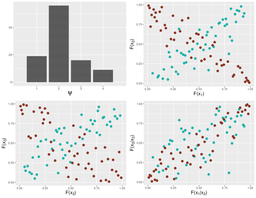
Figure 4: Results from the first scenario, with 100 samples drawn from a $3$-dimensional two-component mixture of conditional Gaussian vine copulas. The covariate was generated from a N(1, 0.5) using the first calibration function with parameters $\boldsymbol{\beta}|(\psi=1)=(\beta_{0_{12}},\beta_{1_{12}},\beta_{0_{23}},\beta_{1_{23}},\beta_{0_{13;2}},\beta_{1_{13;2}})=(1,0.5,0.5,0.3,0.5,0.5)$ and $\boldsymbol{\beta}|(\psi=2)=(\beta_{0_{12}},\beta_{1_{12}},\beta_{0_{23}},\beta_{1_{23}},\beta_{0_{13;2}},\beta_{1_{13;2}})=(-1,-0.5,-0.5,-0.3,0.5,0.5)$. The top left panel shows the barplot of the mode of the number of observed mixture components. The top right and the bottom panels show the scatterplots of the simulated u-data for one of the 100 samples; the blue points denote the observations simulated from the first component $\psi=1$, while the brown points denote the observations simulated from the second component $\psi=2$.

In order to demonstrate the flexibility of our approach for density estimation, we compared simulated and predicted samples. More precisely, in the second, third and fourth scenarios, we generated data from conditional vine copulas constructed with various copula families and different parameters. In these three scenarios, we adopted the first calibration function, simulating the covariate from a N(1, 1). The results are presented in Figures 5, 6 and 7, where the scatterplots show the simulated u-data samples, while the 3-D histograms show the predicted u-data samples.

Figure 5 illustrates the results obtained for scenario 2, where we generated observations from two different two-components mixtures of conditional Gaussian vine copulas. The left panels show the results for a two equally weighted components mixture. The parameters of the calibration function for the first mixture component are

$$\boldsymbol{\beta}|(\psi=1)=(\beta_{0_{12}},\beta_{1_{12}},\beta_{0_{23}},\beta_{1_{23}},\beta_{0_{13;2}},\beta_{1_{13;2}})=(0.4,0.7,-0.3,0.5,-0.1,-0.1)$$

while the parameters for the second component are

$$\boldsymbol{\beta}|(\psi=2)=(\beta_{0_{12}},\beta_{1_{12}},\beta_{0_{23}},\beta_{1_{23}},\beta_{0_{13;2}},\beta_{1_{13;2}})=(-0.4,-0.7,0.5,-0.3,0.1,0.1).$$

The right panels show the results for another two components mixture with equal weights and parameters

$$\boldsymbol{\beta}|(\psi=1)=(\beta_{0_{12}},\beta_{1_{12}},\beta_{0_{23}},\beta_{1_{23}},\beta_{0_{13;2}},\beta_{1_{13;2}})=(1,0.4,-0.8,0.5,-0.3,-0.2)$$

for the first component, and parameters

$$\boldsymbol{\beta}|(\psi=2)=(\beta_{0_{12}},\beta_{1_{12}},\beta_{0_{23}},\beta_{1_{23}},\beta_{0_{13;2}},\beta_{1_{13;2}})=(-0.4,-0.3,0,0.5,0.1,0.1)$$

for the second component. The results show a good performance in terms of density estimation for the proposed methodology in the Gaussian case.

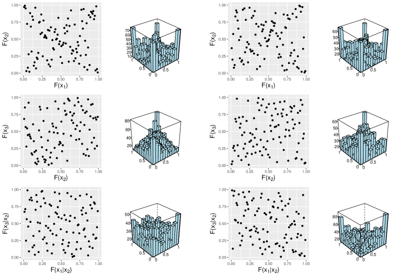
Figure 5: Results from the second scenario, where scatterplots show simulated u-data and 3-D histograms show the predicted u-data. The covariate was generated from a N(1, 1) using the first calibration function. The left panels depict the results for a two equally weighted components mixture of conditional Gaussian vine copulas with parameters $\boldsymbol{\beta}|(\psi=1)=(\beta_{0_{12}},\beta_{1_{12}},\beta_{0_{23}},\beta_{1_{23}},\beta_{0_{13;2}},\beta_{1_{13;2}})=(0.4,0.7,-0.3,0.5,-0.1,-0.1)$ and $\boldsymbol{\beta}|(\psi=2)=(\beta_{0_{12}},\beta_{1_{12}},\beta_{0_{23}},\beta_{1_{23}},\beta_{0_{13;2}},\beta_{1_{13;2}})=(-0.4,-0.7,0.5,-0.3,0.1,0.1)$. The right panels depict the results of a two components mixture of conditional Gaussian vine copulas with equal weights and parameters $\boldsymbol{\beta}|(\psi=1)=(\beta_{0_{12}},\beta_{1_{12}},\beta_{0_{23}},\beta_{1_{23}},\beta_{0_{13;2}},\beta_{1_{13;2}})=(1,0.4,-0.8,0.5,-0.3,-0.2)$ and $\boldsymbol{\beta}|(\psi=2)=(\beta_{0_{12}},\beta_{1_{12}},\beta_{0_{23}},\beta_{1_{23}},\beta_{0_{13;2}},\beta_{1_{13;2}})=(-0.4,-0.3,0,0.5,0.1,0.1)$.

Figure 6 shows the results obtained for scenario 3, where observations were generated from a two equally weighted components mixture of conditional Clayton vine copulas (left panels), and from a two equally weighted components mixture of conditional Gumbel vine copulas (right panel). The parameters of the conditional Clayton vine copula mixture are

$$\boldsymbol{\beta}|(\psi=1)=(\beta_{0_{12}},\beta_{1_{12}},\beta_{0_{23}},\beta_{1_{23}},\beta_{0_{13;2}},\beta_{1_{13;2}})=(0.3,0.7,0,0.5,0.2,0),$$

for the first component and

$$\boldsymbol{\beta}|(\psi=2)=(\beta_{0_{12}},\beta_{1_{12}},\beta_{0_{23}},\beta_{1_{23}},\beta_{0_{13;2}},\beta_{1_{13;2}})=(0.3,0.2,0,0.1,0.2,0),$$

for the second component. The parameters of the conditional Gumbel vine copula mixture are

$$\boldsymbol{\beta}|(\psi=1)=(\beta_{0_{12}},\beta_{1_{12}},\beta_{0_{23}},\beta_{1_{23}},\beta_{0_{13;2}},\beta_{1_{13;2}})=(1.3,0.7,1.0,0.5,1.2,0),$$

for the first component and

$$\boldsymbol{\beta}|(\psi=2)=(\beta_{0_{12}},\beta_{1_{12}},\beta_{0_{23}},\beta_{1_{23}},\beta_{0_{13;2}},\beta_{1_{13;2}})=(1.3,0.2,1.0,0.1,1.2,0),$$

for the second component. The comparison between simulated and predicted data shows that the methodology provides accurate density estimation results with asymmetric Archimedean copulas, such as the Clayton and Gumbel.

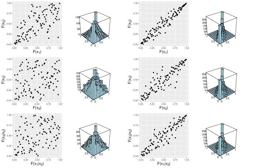
Figure 6: Results from the third scenario, where scatterplots show simulated u-data and 3-D histograms show the predicted u-data. The covariate was generated from a N(1, 1) using the first calibration function. The left panels depict the results for a two equally weighted components mixture of conditional Clayton vine copulas with parameters $\boldsymbol{\beta}|(\psi=1)=(\beta_{0_{12}},\beta_{1_{12}},\beta_{0_{23}},\beta_{1_{23}},\beta_{0_{13;2}},\beta_{1_{13;2}})=(0.3,0.7,0,0.5,0.2,0)$ and $\boldsymbol{\beta}|(\psi=2)=(\beta_{0_{12}},\beta_{1_{12}},\beta_{0_{23}},\beta_{1_{23}},\beta_{0_{13;2}},\beta_{1_{13;2}})=(0.3,0.2,0,0.1,0.2,0)$. The right panels depict the results of a two-component mixture of conditional Gumbel vine copulas with equal weights and parameters $\boldsymbol{\beta}|(\psi=1)=(\beta_{0_{12}},\beta_{1_{12}},\beta_{0_{23}},\beta_{1_{23}},\beta_{0_{13;2}},\beta_{1_{13;2}})=(1.3,0.7,1.0,0.5,1.2,0)$ and $\boldsymbol{\beta}|(\psi=2)=(\beta_{0_{12}},\beta_{1_{12}},\beta_{0_{23}},\beta_{1_{23}},\beta_{0_{13;2}},\beta_{1_{13;2}})=(1.3,0.2,1.0,0.1,1.2,0)$.

The results of scenario 4 are illustrated in Figure 7, where observations were generated from conditional vines constructed with Clayton copulas and their rotated versions. On the left panels we present results from a conditional Clayton vine copula with parameters

$$\boldsymbol{\beta}=(\beta_{0_{12}},\beta_{1_{12}},\beta_{0_{23}},\beta_{1_{23}},\beta_{0_{13;2}},\beta_{1_{13;2}})=(1,0.2,0.8,0.3,0.4,0.1).$$

On the right panels we present results from a conditional vine with rotated Clayton copulas in the first tree and a Clayton copula in the second tree, assuming the following parameters

$$\boldsymbol{\beta}=(\beta_{0_{12}},\beta_{1_{12}},\beta_{0_{23}},\beta_{1_{23}},\beta_{0_{13;2}},\beta_{1_{13;2}})=(-1.5,-0.4,-0.9,-0.8,0.4,0.6).$$

The asymmetric dependence expressed by Clayton and rotated Clayton vines is well captured by the proposed model, as it is clear by comparing simulated and predicted data.

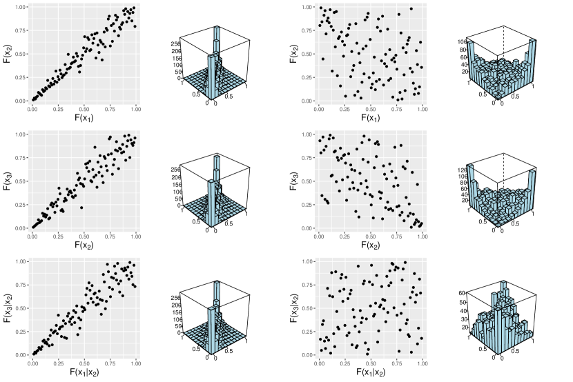
Figure 7: Results from the fourth scenario, where scatterplots show simulated u-data and 3-D histograms show the predicted u-data. The covariate was generated from a N(1, 1) using the first calibration function. The left panels depict the results for a conditional Clayton vine copula with parameters $\boldsymbol{\beta}=(\beta_{0_{12}},\beta_{1_{12}},\beta_{0_{23}},\beta_{1_{23}},\beta_{0_{13;2}},\beta_{1_{13;2}})=(1,0.2,0.8,0.3,0.4,0.1)$. The right panels depict the results for a conditional vine with rotated Clayton copulas in the first tree and a Clayton copula in the second tree, with parameters $\boldsymbol{\beta}=(\beta_{0_{12}},\beta_{1_{12}},\beta_{0_{23}},\beta_{1_{23}},\beta_{0_{13;2}},\beta_{1_{13;2}})=(-1.5,-0.4,-0.9,-0.8,0.4,0.6)$.

In the fifth scenario, the covariate was generated from a N(0.2, 0.1), adopting the second calibration function. The results are presented in Figure 8, where the scatterplots show the simulated u-data samples, while the 3-D histograms show the predicted u-data samples. The left panels illustrate the results obtained generating samples from a conditional Frank vine copula with parameters

$$\boldsymbol{\beta}=(\beta_{0_{12}},\beta_{1_{12}},\beta_{2_{12}},\beta_{3_{12}},\beta_{0_{23}},\beta_{1_{23}},\beta_{2_{23}},\beta_{3_{23}},\beta_{0_{13;2}},\beta_{1_{13;2}},\beta_{2_{13;2}},\beta_{4_{13;2}})\\ =(0.7,0.3,0.2,0.1,0.4,0.3,0.1,0.2,0.2,0.4,0.3,0.5).$$

The right panels show the results obtained generating samples from a conditional vine with rotated Gumbel copulas in the first tree and a Gumbel copula in the second three, assuming the following parameters

$$\boldsymbol{\beta}=(\beta_{0_{12}},\beta_{1_{12}},\beta_{2_{12}},\beta_{3_{12}},\beta_{0_{23}},\beta_{1_{23}},\beta_{2_{23}},\beta_{3_{23}},\beta_{0_{13;2}},\beta_{1_{13;2}},\beta_{2_{13;2}},\beta_{4_{13;2}})\\ =(-0.3,-0.4,-0.1,0.3,-0.5,-0.6,-0.5,0.8,1,-0.1,0.4,-0.3).$$

The results of Figure 8 demonstrate the accuracy of our model for density estimation using the second calibration function. In all the five considered scenarios, the predictive samples generated from the model parameters in most of the cases replicate perfectly the observations.

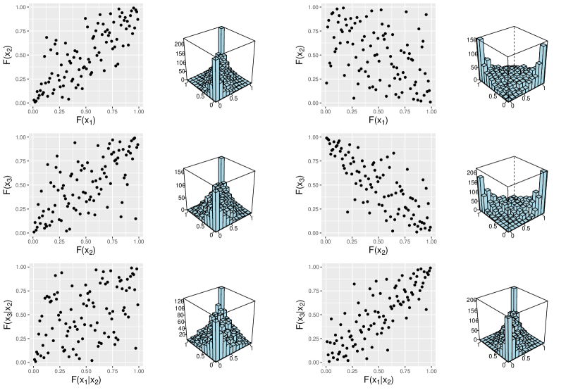
Figure 8: Results from the fifth scenario, where scatterplots show simulated u-data and 3-D histograms show the predicted u-data. The covariate was generated from a N(0.2, 0.1) using the second calibration function. The left panels depict the results for a conditional Frank vine copula with parameters $\boldsymbol{\beta}=(\beta_{0_{12}},\beta_{1_{12}},\beta_{2_{12}},\beta_{3_{12}},\beta_{0_{23}},\beta_{1_{23}},\beta_{2_{23}},\beta_{3_{23}},\beta_{0_{13;2}},\beta_{1_{13;2}},\beta_{2_{13;2}},\beta_{4_{13;2}})=(0.7,0.3,0.2,0.1,0.4,0.3,0.1,0.2,0.2,0.4,0.3,0.5)$. The right panels depict the results for a conditional vine with rotated Gumbel copulas in the first tree and a Gumbel copula in the second tree, with parameters $\boldsymbol{\beta}=(\beta_{0_{12}},\beta_{1_{12}},\beta_{2_{12}},\beta_{3_{12}},\beta_{0_{23}},\beta_{1_{23}},\beta_{2_{23}},\beta_{3_{23}},\beta_{0_{13;2}},\beta_{1_{13;2}},\beta_{2_{13;2}},\beta_{4_{13;2}})=(-0.3,-0.4,-0.1,0.3,-0.5,-0.6,-0.5,0.8,1,-0.1,0.4,-0.3)$.

5.2 Financial Development and Natural Disasters

We now present the application of the proposed methodology to a heterogeneous dataset to study the impacts of worldwide natural disasters on international financial development.

In recent years several authors in the literature have focused on the relationship between economic growth and natural disasters. Toya and Skidmore (2007) show that countries with higher income, higher educational attainment, greater openness, more advanced financial systems and smaller governments tend to suffer fewer losses in presence of natural disasters. Felbermayr and Gröschl (2014) built a comprehensive database of disaster events and their intensities from primary geophysical and meteorological information, revealing a substantial negative and robust average impact effect of disasters on growth. So far, researchers have mostly dealt with financial development studies using several proxies as measures of financial depth, such as the ratio of private credit to GDP or stock market capitalization to GDP. For example, Keerthiratne and Tol (2017) proposed an empirical analysis of the effect of the occurrence of natural disasters on financial development proxies. However, this approach does not take into account the complex nature of financial developments. The International Monetary Fund (IFM) provides, for each country, the Financial Development (FD) index, which summarizes how developed financial institutions and financial markets are in that specific country. The index considers several factors, such as size and liquidity of the markets, ability of individuals and companies to access financial services, ability of institutions to provide financial services at low cost and with sustainable revenues and level of activity of the capital markets. We constructed a dataset merging information from the IFM and the Emergency Events Database and we analyzed the impact of natural disasters on the dependence between the FD index values in several years. In particular, we investigated how the occurrence of a natural disaster affects the time dependence between the FD index values in the four years following the disaster.

The original data included observations of the FD index (expressed in percentages) in 181 countries from 1980 to 2019 with annual frequency. We are interested in the effect of a single natural disaster on the FD index in the 4 years following the event. Note that, if in the considered 4 years interval more that one natural disaster occurred, the observation was discarded. Based on the original data, we constructed a study dataset where each observation corresponds to a set of 4 consecutive year periods affected by a natural disaster in the first year. Hence, each country may be represented by more than one observation. Our final study data comprises $N=525$ observations (for $n=86$ different countries) and four variables containing the FD indexes for each one of the 4 considered years. The dataset is structured as reported in Table 1, where $t_{i}$ denotes the number of time periods for each country, with $j=1,\ldots,t_{i}$ and $i$ denotes the country, with $i=1,\ldots,n=86$.

Table 1: Financial development data structure.

Country	Time	FD index	FD index	FD index	FD index
	period	at time 1	at time 2	at time 3	at time 4
1	1	$y_{1,1}$	$y_{1,1+1}$	$y_{1,1+2}$	$y_{1,1+3}$
1	2	$y_{1,2}$	$y_{1,2+1}$	$y_{1,2+2}$	$y_{1,2+3}$
⋮	⋮	⋮	⋮	⋮	⋮
1	$t_{1}$	$y_{1,t_{1}}$	$y_{1,t_{1}+1}$	$y_{1,t_{1}+2}$	$y_{1,t_{1}+3}$
2	1	$y_{2,1}$	$y_{2,1+1}$	$y_{2,1+2}$	$y_{2,1+3}$
2	2	$y_{2,2}$	$y_{2,2+1}$	$y_{2,2+2}$	$y_{2,2+3}$
⋮	⋮	⋮	⋮	⋮	⋮
2	$t_{2}$	$y_{2,t_{2}}$	$y_{2,t_{2}+1}$	$y_{2,t_{2}+2}$	$y_{2,t_{2}+3}$
…	…	…	…	…	…
$n$	1	$y_{n,1}$	$y_{n,1+1}$	$y_{n,1+2}$	$y_{n,1+3}$
$n$	2	$y_{n,2}$	$y_{n,2+1}$	$y_{n,2+2}$	$y_{n,2+3}$
⋮	⋮	⋮	⋮	⋮	⋮
$n$	$t_{n}$	$y_{n,t_{n}}$	$y_{n,t_{n}+1}$	$y_{n,t_{n}+2}$	$y_{n,t_{n}+3}$

We applied the proposed Bayesian nonparametric unconditional vine mixture approach to the study dataset, constructing a $4$-dimensional vine copula, with marginals denoting the FD index in $4$ consecutive years. The adoption of an infinite mixture approach allows us to control for both individual and temporal heterogeneity in the dataset.

Since the marginal variables $(y_{i,t_{i}},y_{i,t_{i}+1},y_{i,t_{i}+2},y_{i,t_{i}+3})$, with $i=1,\ldots,n$, are expressed in percentages, they are defined on the support $\left[0,1\right]$. Hence, we assume the marginal distributions to be independent $\text{Beta}(a_{j},b_{j})$ with $a_{j}$ and $b_{j}$ defined a priori $\text{Gamma}(1,1)$ for $j=1,\dots,4$. Inference for the margins is separately performed via Metropolis-Hastings. Results are reported in Table 2.

Table 2: Financial development and natural disasters analysis: mean, standard deviation and credibility intervals for the posterior densities of the marginal parameters.

	$a_{{1}}$	$b_{{1}}$	$a_{{2}}$	$b_{{2}}$	$a_{{3}}$	$b_{{3}}$	$a_{{4}}$	$b_{{4}}$
$E(\cdot|y)$	2.05	3.82	2.17	3.85	2.20	3.76	2.19	3.64
$SD(\cdot|y)$	0.11	0.23	0.13	0.25	0.13	0.23	0.12	0.21
$q_{0.025}(\cdot|y)$	1.83	3.38	1.92	3.39	1.95	3.31	1.95	3.22
$q_{0.975}(\cdot|y)$	2.28	4.28	2.43	4.33	2.45	4.21	2.44	4.08

We consider the occurrence of a natural disaster to be a covariate in our conditional vine copula model. Since natural disasters are defined basing on their intensity, which is measured using the total damage as proxy variable, we constructed the binary covariate taking value $X=1$ if the total damage is over 100 million dollars and $X=0$ otherwise. Since the model requires a distributional assumption on the covariate, we defined $X\sim\text{Bernoulli}(\phi)$ assuming a priori $\phi\sim\text{Beta}(a_{\phi},b_{\phi})$. Moreover, we chose a linear calibration function for each pair copula $\eta_{s}(x|\boldsymbol{\beta})=\beta_{0_{s}}+\beta_{1_{s}}x$, where $s=1,\dots,6$ denotes the pair-copulas in the vine. For the definition of kernel of the mixture we adopt a D-vine approach, since this specific type of vine better describes temporal sequences and easily takes the time ordering of consecutive events into account (Barthel et al., 2019). We therefore consider a $4$-dimensional D-vine, where the marginals are the FD indexes of the 4 consecutive years and with covariate given by the natural disaster intensity. We set the total mass parameter as $M=1$ and define the centering measure as

$$G_{0}\equiv\text{Beta}\left(a_{\phi},b_{\phi}\right)\times\mathbb{N}_{(6\times 2)}(\boldsymbol{\mu},\boldsymbol{\Sigma}).$$

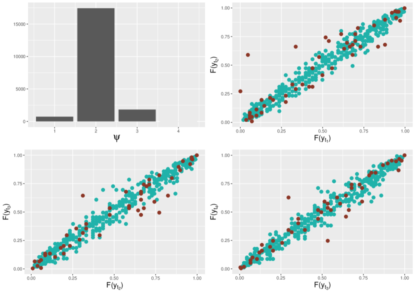
Figure 9: Results from the financial development and natural disasters analysis. The top left panel shows the barplot of the mode of the number of observed mixture components. The top right and the bottom panels show the scatterplots of the observed u-data for the first vine tree; the blue points denote the observations belonging to the first cluster $\psi=1$, while the brown points denote the observations belonging to the second cluster $\psi=2$.

Our approach estimates two clusters, as shown in Figure 9. The top left panel shows the barplot of the mode of the number of observed mixture components. The other panels show the scatterplots of the observed u-data for the first vine tree; more precisely, the scatterplot of the first and second time periods are shown in the top right panel, the scatterplot of the second and third time periods are shown in the bottom left panel, while the scatterplot of the third and fourth time periods are shown in the bottom right panel. The blue points denote the observations belonging to the first cluster $\psi=1$, while the brown points denote the observations belonging to the second cluster $\psi=2$.

In Table 3 we report the resulting mean, standard deviation and credibility intervals for the posterior densities of the calibration functions parameters. The top part of the table shows the results for the first cluster $\psi=1$, while the bottom part shows the results of the second cluster $\psi=2$.

Table 3: Financial development and natural disasters analysis: mean, standard deviation and credibility intervals for the posterior densities of the calibration function parameters. The top part of the table shows the results for the first cluster $\psi=1$, while the bottom part shows the results of the second cluster $\psi=2$.

$\psi=1$	$\beta_{0_{12}}$	$\beta_{1_{12}}$	$\beta_{0_{23}}$	$\beta_{1_{23}}$	$\beta_{0_{34}}$	$\beta_{1_{34}}$	$\beta_{0_{13;2}}$	$\beta_{1_{13;2}}$	$\beta_{0_{24;3}}$	$\beta_{1_{24;3}}$	$\beta_{0_{14;2,3}}$	$\beta_{1_{14;2,3}}$
$E(\cdot|y,x)$	2.40	-0.63	2.31	-0.49	2.36	-0.81	-0.06	0.08	-0.08	0.07	-0.09	0.41
$SD(\cdot|y,x)$	0.08	0.33	0.05	0.42	0.05	0.36	0.06	0.33	0.06	0.26	0.06	0.34
$q_{0.025}(\cdot|y,x)$	2.23	-1.34	2.23	-1.16	2.26	-1.40	-0.18	-0.64	-0.20	-0.41	-0.20	-0.35
$q_{0.975}(\cdot|y,x)$	2.51	-0.05	2.39	0.62	2.44	0.26	0.06	0.71	0.04	0.62	0.02	1.03
$\psi=2$	$\beta_{0_{12}}$	$\beta_{1_{12}}$	$\beta_{0_{23}}$	$\beta_{1_{23}}$	$\beta_{0_{34}}$	$\beta_{1_{34}}$	$\beta_{0_{13;2}}$	$\beta_{1_{13;2}}$	$\beta_{0_{24;3}}$	$\beta_{1_{24;3}}$	$\beta_{0_{14;2,3}}$	$\beta_{1_{14;2,3}}$
$E(\cdot|y,x)$	0.57	1.91	1.81	0.76	1.88	0.81	0.01	-0.19	-0.08	0.14	-0.13	0.24
$SD(\cdot|y,x)$	0.36	0.38	0.43	0.47	0.62	0.67	0.26	0.32	0.60	0.64	0.32	0.40
$q_{0.025}(\cdot|y,x)$	-0.27	1.14	0.92	-0.04	0.09	-0.28	-0.50	-0.50	-0.86	-1.25	-0.73	-0.43
$q_{0.975}(\cdot|y,x)$	1.19	2.68	2.63	1.72	2.88	2.64	0.49	0.46	0.44	0.94	0.42	1.03

The top left panel of Figure 10 shows the barplot of the number of observations allocated to the two estimated mixture components. The top right panel compares the posterior densities of the calibration function parameter $\beta_{1_{12}}$ (which is related to the first time interval from $t_{i}$ to $t_{i}+1$, with $i=1,\ldots,n$) for the first (blue) and the second (brown) mixture components. The left and right bottom panels show, for the first (blue) and second (brown) mixture components, the boxplots of the calibration function parameters $\beta_{1_{12}}$ (left; first time interval from $t_{i}$ to $t_{i}+1$), $\beta_{1_{23}}$ (middle; second time interval from $t_{i}+1$ to $t_{i}+2$) and $\beta_{1_{34}}$ (right; third time interval from $t_{i}+2$ to $t_{i}+3$) for the first vine tree. Figure 10 reveals that the two mixture components present substantial differences in terms of how they are impacted by natural disasters. For the first cluster ($\psi=1$) the model estimates a general negative effect which tends to remain constant until the fourth year; instead, for the second cluster ($\psi=2$) the model estimates a positive effect of the natural disaster on the time dependence between yearly FD indexes.

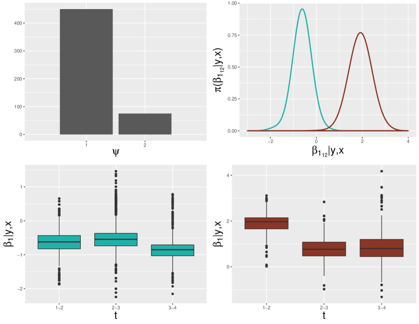
Figure 10: Results from the financial development and natural disasters analysis. The top left panel shows the barplot of the number of observations allocated to the two estimated mixture components. The top right panel compares the posterior densities of the calibration function parameter $\beta_{1_{12}}$ (which is related to the first time interval from $t_{i}$ to $t_{i}+1$, with $i=1,\ldots,n$) for the first (blue) and the second (brown) mixture components. The left and right bottom panels show, for the first (blue) and second (brown) mixture components, the boxplots of the calibration function parameters $\beta_{1_{12}}$ (left; first time interval from $t_{i}$ to $t_{i}+1$), $\beta_{1_{23}}$ (middle; second time interval from $t_{i}+1$ to $t_{i}+2$) and $\beta_{1_{34}}$ (right; third time interval from $t_{i}+2$ to $t_{i}+3$) for the first vine tree.

Table 4: Financial development and natural disasters analysis. The left table shows the mean, standard deviation and credibility intervals for the posterior densities of the covariate parameter for the two estimated mixture components ($\psi=1$ in the left column, $\psi=2$ in the right column). The right table shows the same statistics for the mixture weights of the two estimated mixture components ($\psi=1$ in the left column, $\psi=2$ in the right column).

	$\psi=1$	$\psi=2$
$E(\phi|x)$	0.03	0.84
$SD(\phi|x)$	0.01	0.07
$q_{0.025}(\phi|x)$	0.01	0.06
$q_{0.975}(\phi|x)$	0.70	0.97

	$w_{1}$	$w_{2}$
$E(\cdot|y,x)$	0.85	0.15
$SD(\cdot|y,x)$	0.02	0.02
$q_{0.025}(\cdot|y,x)$	0.81	0.11
$q_{0.975}(\cdot|y,x)$	0.89	0.19

Let $w_{1}$ and $w_{2}$ be the mixture weights for the two estimated components, i.e. the variables indicating the proportion of observations belonging to each group. Table 4 shows, on the left, the mean, standard deviation and credibility intervals for the posterior densities of the covariate parameter for the two estimated mixture components ($\psi=1$ in the left column, $\psi=2$ in the right column). On the right, Table 4 shows the same statistics for the mixture weights. As reported in Table 4, and in the barplot of Figure 10, the $85\%$ of the observations belong to the first cluster, meaning that in most of the cases natural disasters are expected to have negatively affect the financial development. However, from Table 4 we can get another interesting point: the expected value of the posterior probability of natural disasters $E(\phi|x)$ is very low in the first and very high in the second cluster. This result may give a further intuition: the less a natural disaster was expected, the less the government was prepared for that event. On the contrary, if the occurrence of a natural disaster was more expected, governments and financial institutions were prepared for that event and were able to face the possible effects on the financial structure of the country. In Table 5 we report the list of countries, years and type of natural disasters which had an estimated positive effect on the FD index.

Table 5: List of countries, years and type of natural disasters which had an estimated positive effect on the FD index.

Country	$t$	Category of disaster	Type of disaster
Burundi	2015	Hydrological	Landslide
Benin	1980	Climatological	Drought
Bulgaria	2007	Meteorological	Extreme temperature
Barbados	1980	Meteorological	Storm
Switzerland	1994	Meteorological	Storm
Switzerland	1990	Meteorological	Storm
Costa Rica	2012	Hydrological	Flood
Cyprus	1995	Geophysical	Earthquake
Denmark	1999	Meteorological	Storm
Denmark	1992	Climatological	Drought
Estonia	2005	Meteorological	Storm
Georgia	2004	Hydrological	Flood
Grenada	1999	Meteorological	Storm
Croatia	2000	Hydrological	Flood
Ireland	2011	Hydrological	Flood
Iceland	2000	Geophysical	Earthquake
Iceland	1996	Geophysical	Volcanic activity
Israel	2010	Hydrological	Flood
Israel	2000	Meteorological	Extreme temperature
Israel	1992	Meteorological	Extreme temperature
Italy	2003	Hydrological	Flood
Jamaica	1980	Meteorological	Storm
Kazakhstan	2005	Hydrological	Flood
Luxembourg	1990	Meteorological	Storm
Latvia	2005	Meteorological	Storm

Country	$t$	Category of disaster	Type of disaster
Madagascar	1994	Meteorological	Storm
Madagascar	1986	Meteorological	Storm
Mongolia	2009	Hydrological	Flood
Mongolia	2003	Hydrological	Flood
Mauritius	2002	Meteorological	Storm
Norway	2005	Meteorological	Storm
Norway	1995	Hydrological	Flood
Norway	1990	Meteorological	Storm
Panama	1995	Hydrological	Flood
Poland	2002	Meteorological	Storm
Poland	1990	Meteorological	Storm
Poland	1987	Hydrological	Flood
Portugal	2010	Hydrological	Flood
Portugal	1997	Meteorological	Storm
Portugal	1985	Climatological	Wildfire
Sweden	2005	Meteorological	Storm
Sweden	1999	Meteorological	Storm
Sweden	1990	Meteorological	Storm
Trinidad and Tobago	1993	Hydrological	Flood
Turkey	2011	Geophysical	Earthquake
Turkey	1980	Hydrological	Landslide
Ukraine	2013	Hydrological	Flood
Ukraine	2001	Hydrological	Flood
Uruguay	2002	Meteorological	Storm

6 Concluding Remarks

In this paper we introduce a novel approach for multivariate distributions, which takes advantage of vine specifications. Vines are very flexible constructions that express multidimensional copulas as building blocks. This specification allows us to easily incorporate covariates driving the dependence between the response variables. Inference is carried out following the Bayesian nonparametrics approach, assuming a DP prior distribution on the mixing measure of an infinite mixture of conditional vine copulas. One of the benefits of this approach is that the specification of copula families for each pair copula is not required. Another benefit is that this approach allows us to model individual as well as temporal heterogeneity in a natural way. Our methodology exhibits an excellent performance in simulation studies for both clustering and density estimation. We also demonstrate the power of the proposed approach applying it to a dataset which investigates the effects of natural disasters on the financial development of a number of countries worldwide. The proposed Bayesian nonparametric approach for conditional vine mixtures allows us to capture the unobserved heterogeneity that is intrinsic in the dataset. The results show the presence of two distinct country clusters with opposite behaviour in terms of reaction to natural hazards.

References

- Aas et al. [2009] Kjersti Aas, Claudia Czado, Arnoldo Frigessi, and Henrik Bakken. Pair-copula constructions of multiple dependence. Insurance: Mathematics and economics, 44(2):182–198, 2009.
- Abegaz et al. [2012] Fentaw Abegaz, Irène Gijbels, and Noël Veraverbeke. Semiparametric estimation of conditional copulas. Journal of Multivariate Analysis, 110:43–73, 2012.
- Acar et al. [2011] Elif F Acar, Radu V Craiu, and Fang Yao. Dependence calibration in conditional copulas: A nonparametric approach. Biometrics, 67(2):445–453, 2011.
- Barthel et al. [2019] Nicole Barthel, Candida Geerdens, Claudia Czado, and Paul Janssen. Dependence modeling for recurrent event times subject to right-censoring with d-vine copulas. Biometrics, 75(2):439–451, 2019.
- Bartram et al. [2007] Söhnke M Bartram, Stephen J Taylor, and Yaw-Huei Wang. The euro and european financial market dependence. Journal of Banking & Finance, 31(5):1461–1481, 2007.
- Bedford and Cooke [2001] Tim Bedford and Roger M Cooke. Probability density decomposition for conditionally dependent random variables modeled by vines. Annals of Mathematics and Artificial intelligence, 32(1-4):245–268, 2001.
- Bermúdez et al. [2020] Lluís Bermúdez, Dimitris Karlis, and Isabel Morillo. Modelling unobserved heterogeneity in claim counts using finite mixture models. Risks, 8(1):10, 2020.
- Buddhavarapu et al. [2016] Prasad Buddhavarapu, James G Scott, and Jorge A Prozzi. Modeling unobserved heterogeneity using finite mixture random parameters for spatially correlated discrete count data. Transportation Research Part B: Methodological, 91:492–510, 2016.
- Craiu and Sabeti [2012] V Radu Craiu and Avideh Sabeti. In mixed company: Bayesian inference for bivariate conditional copula models with discrete and continuous outcomes. Journal of Multivariate Analysis, 110:106–120, 2012.
- Czado [2019] Claudia Czado. Analyzing Dependent Data with Vine Copulas. Springer, 2019.
- Dalla Valle et al. [2018] Luciana Dalla Valle, Fabrizio Leisen, and Luca Rossini. Bayesian non-parametric conditional copula estimation of twin data. Journal of the Royal Statistical Society: Series C (Applied Statistics), 67(3):523–548, 2018.
- Fan and Patton [2014] Yanqin Fan and Andrew J Patton. Copulas in econometrics. Annu. Rev. Econ., 6(1):179–200, 2014.
- Felbermayr and Gröschl [2014] Gabriel Felbermayr and Jasmin Gröschl. Naturally negative: The growth effects of natural disasters. Journal of development economics, 111:92–106, 2014.
- Genest et al. [2009] Christian Genest, Michel Gendron, and Michaël Bourdeau-Brien. The advent of copulas in finance. The European Journal of Finance, 15(7-8):609–618, 2009.
- Gijbels et al. [2011] Irène Gijbels, Noël Veraverbeke, and Marel Omelka. Conditional copulas, association measures and their applications. Computational Statistics & Data Analysis, 55(5):1919–1932, 2011.
- Gijbels et al. [2012] Irene Gijbels, Marek Omelka, Noël Veraverbeke, et al. Multivariate and functional covariates and conditional copulas. Electronic Journal of Statistics, 6:1273–1306, 2012.
- Grazian and Liseo [2017] Clara Grazian and Brunero Liseo. Approximate bayesian inference in semiparametric copula models. Bayesian Analysis, 12(4):991–1016, 2017.
- Grazian et al. [2021] Clara Grazian, Luciana Dalla Valle, and Brunero Liseo. Approximate bayesian conditional copulas. arXiv preprint arXiv:2103.02974, 2021.
- Green and Richardson [2001] Peter J Green and Sylvia Richardson. Modelling heterogeneity with and without the dirichlet process. Scandinavian journal of statistics, 28(2):355–375, 2001.
- Jedidi et al. [1997] Kamel Jedidi, Harsharanjeet S Jagpal, and Wayne S DeSarbo. Finite-mixture structural equation models for response-based segmentation and unobserved heterogeneity. Marketing Science, 16(1):39–59, 1997.
- Joe [1996] Harry Joe. Families of m-variate distributions with given margins and m (m-1)/2 bivariate dependence parameters. Lecture Notes-Monograph Series, pages 120–141, 1996.
- Joe [2014] Harry Joe. Dependence modeling with copulas. CRC press, 2014.
- Jondeau and Rockinger [2006] Eric Jondeau and Michael Rockinger. The copula-garch model of conditional dependencies: An international stock market application. Journal of international money and finance, 25(5):827–853, 2006.
- Kalli et al. [2011] Maria Kalli, Jim E Griffin, and Stephen G Walker. Slice sampling mixture models. Statistics and computing, 21(1):93–105, 2011.
- Keerthiratne and Tol [2017] Subhani Keerthiratne and Richard SJ Tol. Impact of natural disasters on financial development. Economics of Disasters and Climate Change, 1(1):33–54, 2017.
- Kolev et al. [2006] Nikolai Kolev, Ulisses dos Anjos, and Beatriz Vaz de M Mendes. Copulas: a review and recent developments. Stochastic models, 22(4):617–660, 2006.
- Kurowicka and Cooke [2006] Dorota Kurowicka and Roger M Cooke. Uncertainty analysis with high dimensional dependence modelling. John Wiley & Sons, 2006.
- MacEachern and Müller [1998] Steven N MacEachern and Peter Müller. Estimating mixture of dirichlet process models. Journal of Computational and Graphical Statistics, 7(2):223–238, 1998.
- Morgan and Ridout [2008] Byron JT Morgan and Martin S Ridout. A new mixture model for capture heterogeneity. Journal of the Royal Statistical Society: Series C (Applied Statistics), 57(4):433–446, 2008.
- Müller and Quintana [2010] Peter Müller and Fernando Quintana. Random partition models with regression on covariates. Journal of statistical planning and inference, 140(10):2801–2808, 2010.
- Müller and Rosner [1997] Peter Müller and Gary L Rosner. A bayesian population model with hierarchical mixture priors applied to blood count data. Journal of the American Statistical Association, 92(440):1279–1292, 1997.
- Nelsen [2007] Roger B Nelsen. An introduction to copulas. Springer Science & Business Media, 2007.
- Patton [2006] Andrew J Patton. Modelling asymmetric exchange rate dependence. International economic review, 47(2):527–556, 2006.
- Sklar [1959] A Sklar. Fonctions dé repartition à n dimension et leurs marges. Université Paris, 8(3.2):1–3, 1959.
- Toya and Skidmore [2007] Hideki Toya and Mark Skidmore. Economic development and the impacts of natural disasters. Economics letters, 94(1):20–25, 2007.
- Turek et al. [2021] Daniel Turek, Claudia Wehrhahn, and Olivier Gimenez. Bayesian non-parametric detection heterogeneity in ecological models. Environmental and Ecological Statistics, 28(2):355–381, 2021.
- Walker [2007] Stephen G Walker. Sampling the dirichlet mixture model with slices. Communications in Statistics—Simulation and Computation®, 36(1):45–54, 2007.
- Wu et al. [2014] Juan Wu, Xue Wang, and Stephen G Walker. Bayesian nonparametric inference for a multivariate copula function. Methodology and Computing in Applied Probability, 16(3):747–763, 2014.
- Wu et al. [2015] Juan Wu, Xue Wang, and Stephen G Walker. Bayesian nonparametric estimation of a copula. Journal of Statistical Computation and Simulation, 85(1):103–116, 2015.
- Zhang and Wang [2018] Susu Zhang and Shiyu Wang. Modeling learner heterogeneity: A mixture learning model with responses and response times. Frontiers in psychology, 9:2339, 2018.
- Zhuang et al. [2021] Haoxin Zhuang, Liqun Diao, and Y Yi Grace. A bayesian nonparametric mixture model for grouping dependence structures and selecting copula functions. Econometrics and Statistics, 2021.